SELFISH ROUTING

A Dissertation

Presented to the Faculty of the Graduate School

of Cornell University

in Partial Fulfillment of the Requirements for the Degree of

Doctor of Philosophy

by

Tim Roughgarden

May 2002

c© Tim Roughgarden 2002

ALL RIGHTS RESERVED

SELFISH ROUTING

Tim Roughgarden, Ph.D.

Cornell University 2002

A central and well-studied problem arising in the management of a large networkis that of routing traffic to achieve the best possible network performance. In manynetworks, it is difficult or even impossible to impose optimal routing strategies onnetwork traffic, leaving network users free to act according to their own interests.In general, the result of local optimization by many selfish network users with con-flicting interests does not possess any type of global optimality; hence, this lack ofregulation carries the cost of decreased network performance.

We study the degradation in network performance due to selfish, uncoordinatedbehavior by network users. Our contributions are twofold: we quantify the worst-possible loss in network performance arising from noncooperative behavior; and wedesign and analyze algorithms for building and managing networks so that selfishbehavior leads to a socially desirable outcome.

To quantify the loss in network performance caused by selfish behavior, we in-vestigate the following question: what is the worst-case ratio between the social costof an uncoordinated outcome and the social cost of the best coordinated outcome?We provide an exact solution to this problem in a variety of traffic models, therebyidentifying types of networks for which the cost of routing selfishly is mild.

The inefficiency inherent in an uncoordinated outcome and the inability to cen-trally implement a globally optimal solution motivate our second question: howcan we ensure that the loss in network performance due to selfish behavior will betolerable? We explore two algorithmic approaches to coping with the selfishness ofnetwork users. First, we consider the problem of designing networks that exhibitgood performance when used selfishly. Second, we study how to route a small frac-tion of the traffic centrally to induce “good” (albeit selfish) behavior from the restof the network users. We give both efficient algorithms with provable performanceguarantees and hardness of approximation results for these two problems.

Biographical Sketch

Tim Roughgarden was born on July 20th, 1975. He received a B.S. in Applied

Mathematics and Environmental Science from Stanford University in June 1997,

an M.S. in Computer Science from Stanford University in June 1998, and expects

to receive an M.S. in Mathematics and a Ph.D. in Computer Science from Cornell

University in May 2002.

iii

Acknowledgements

I have been very lucky to learn from a number of outstanding advisors at Cornell

during my graduate studies. First and foremost, I am deeply indebted to my Ph.D.

advisor, Eva Tardos; her insights (technical and otherwise) over the years have been

invaluable to me. I also thank Jon Kleinberg, both for convincing me to come

to Cornell for graduate school, and for his advice on talks, tennis rackets, and

everything in between. I thank David Shmoys for many enjoyable discussions; like

Eva and Jon, David has significantly influenced the way I think about research. I

thank Lou Billera for serving on my committee and for pointers to relevant work in

the game theory community.

I have also been fortunate to experience other exciting research environments

over the past few years. The genesis of this thesis occurred during the 1999-2000

school year, when I was visiting U.C. Berkeley. I will always remember the Theory

Lunch (that I was doubtlessly attending only for the free food) at which Leonard

Schulman described Braess’s Paradox and Christos Papadimitriou proposed compar-

ing the social welfare of selfish and optimal solutions. Leonard and Christos have

my eternal thanks for asking the questions that inspired my dissertation work. I am

also grateful to the researchers at IBM Watson and IBM Almaden, and especially

to David Williamson, for two great summers in the research industry.

Before coming to Cornell, I benefited from a number of mentors at Stanford. I

am especially grateful to Serge Plotkin, who introduced me to the field of algorithms,

got me excited about network flow, and provided support for my masters degree; to

Steve Schneider, who advised my undergraduate thesis and showed me how much

fun research can be; to Eric Roberts, for his contagious enthusiasm about computer

science and inspiring work ethic; and to Gunnar Carlsson, who first introduced me

to mathematical research. Going back even further in time, I am indebted to my

parents for encouraging a love of learning at an early age.

iv

Finally, of all the friends who have helped me out through the years, I’ll single

out only Eve Donnelly for special thanks; she’s had to put up with me the most.

This work was supported by an NSF Fellowship, a Cornell University Fellowship,

and ONR grant N00014-98-1-0589, and was performed in part while visiting the

Department of Computer Science at UC Berkeley and IBM Almaden.

v

vi

Table of Contents

I Overview and Preliminaries 1

1 Introduction 31.1 Selfish Routing . . . . . . . . . . . . . . . . . . . . . . . . . . . . . . 31.2 Two Motivating Examples . . . . . . . . . . . . . . . . . . . . . . . . 4

1.2.1 Pigou’s Example . . . . . . . . . . . . . . . . . . . . . . . . . 41.2.2 Braess’s Paradox . . . . . . . . . . . . . . . . . . . . . . . . . 5

1.3 Our Contributions . . . . . . . . . . . . . . . . . . . . . . . . . . . . 71.3.1 Bounding the Price of Anarchy . . . . . . . . . . . . . . . . . 81.3.2 Braess’s Paradox and Network Design . . . . . . . . . . . . . . 121.3.3 Stackelberg Routing . . . . . . . . . . . . . . . . . . . . . . . 13

1.4 Comparison to Previous Work . . . . . . . . . . . . . . . . . . . . . . 141.5 Tips for Reading this Thesis . . . . . . . . . . . . . . . . . . . . . . . 16

1.5.1 Prerequisites . . . . . . . . . . . . . . . . . . . . . . . . . . . . 161.5.2 Presentation Overview . . . . . . . . . . . . . . . . . . . . . . 161.5.3 Dependencies . . . . . . . . . . . . . . . . . . . . . . . . . . . 17

1.6 Bibliographic Notes . . . . . . . . . . . . . . . . . . . . . . . . . . . . 17

2 Preliminaries 182.1 The Model . . . . . . . . . . . . . . . . . . . . . . . . . . . . . . . . . 182.2 Flows at Nash Equilibrium . . . . . . . . . . . . . . . . . . . . . . . . 202.3 A Characterization of Optimal Flows . . . . . . . . . . . . . . . . . . 212.4 Examples . . . . . . . . . . . . . . . . . . . . . . . . . . . . . . . . . 24

2.4.1 Pigou’s Example . . . . . . . . . . . . . . . . . . . . . . . . . 242.4.2 Braess’s Paradox . . . . . . . . . . . . . . . . . . . . . . . . . 252.4.3 Strict Pareto Suboptimality of Nash without Paradox . . . . . 262.4.4 A Nonlinear Variant of Pigou’s Example . . . . . . . . . . . . 272.4.5 The Unfairness of Optimal Flows . . . . . . . . . . . . . . . . 28

2.5 Existence and Uniqueness of Nash Flows . . . . . . . . . . . . . . . . 292.6 Acyclicity of Nash Flows . . . . . . . . . . . . . . . . . . . . . . . . . 31

vii

II Bounding the Price of Anarchy 34

3 How Bad is Selfish Routing? 363.1 Introduction . . . . . . . . . . . . . . . . . . . . . . . . . . . . . . . . 36

3.1.1 Summary of Results . . . . . . . . . . . . . . . . . . . . . . . 363.1.2 Related Work . . . . . . . . . . . . . . . . . . . . . . . . . . . 383.1.3 Organization . . . . . . . . . . . . . . . . . . . . . . . . . . . 40

3.2 The Price of Anarchy with Linear Latency Functions . . . . . . . . . 413.3 The Price of Anarchy with Standard Latency Functions . . . . . . . . 46

3.3.1 The Anarchy Value . . . . . . . . . . . . . . . . . . . . . . . . 473.3.2 Proof Approach . . . . . . . . . . . . . . . . . . . . . . . . . . 493.3.3 Proof of Upper Bound . . . . . . . . . . . . . . . . . . . . . . 50

3.4 The Price of Anarchy is Independent of the Network Topology . . . . 533.4.1 Lower Bounds in Two-Link Networks . . . . . . . . . . . . . . 533.4.2 Lower Bounds in Networks of Parallel Links . . . . . . . . . . 54

3.5 Computing the Price of Anarchy . . . . . . . . . . . . . . . . . . . . . 563.5.1 More Techniques for Computing the Price of Anarchy . . . . . 563.5.2 Applications . . . . . . . . . . . . . . . . . . . . . . . . . . . . 58

3.6 A Bicriteria Bound for Networks with Arbitrary Latency Functions . 63

4 Extensions to Other Models 684.1 Flows at Approximate Nash Equilibrium . . . . . . . . . . . . . . . . 694.2 Finitely Many Users: Splittable Flow . . . . . . . . . . . . . . . . . . 714.3 Finitely Many Users: Unsplittable Flow . . . . . . . . . . . . . . . . . 734.4 Nonatomic Congestion Games . . . . . . . . . . . . . . . . . . . . . . 75

4.4.1 Definitions . . . . . . . . . . . . . . . . . . . . . . . . . . . . . 764.4.2 Related Work . . . . . . . . . . . . . . . . . . . . . . . . . . . 774.4.3 Bounding the Inefficiency of Nash Equilibria in NCGs . . . . . 78

III Coping with Selfishness 80

5 Designing Networks for Selfish Users 825.1 Introduction . . . . . . . . . . . . . . . . . . . . . . . . . . . . . . . . 82

5.1.1 Summary of Results . . . . . . . . . . . . . . . . . . . . . . . 835.1.2 Related Work . . . . . . . . . . . . . . . . . . . . . . . . . . . 835.1.3 Organization . . . . . . . . . . . . . . . . . . . . . . . . . . . 85

5.2 Encodings of Latency Functions . . . . . . . . . . . . . . . . . . . . . 855.3 Linear Latency Functions:

An Approximability Threshold of 43

. . . . . . . . . . . . . . . . . . . 865.4 General Latency Functions:

An Approximability Threshold of n/2 . . . . . . . . . . . . . . . . . 885.4.1 An n/2-Approximation Algorithm . . . . . . . . . . . . . . 895.4.2 The Braess Graphs . . . . . . . . . . . . . . . . . . . . . . . . 915.4.3 Proof of Hardness . . . . . . . . . . . . . . . . . . . . . . . . . 93

viii

5.5 Polynomials of Bounded Degree:An Approximability Threshold of Θ( p

log p) . . . . . . . . . . . . . . . . 97

6 Stackelberg Routing 1046.1 Introduction . . . . . . . . . . . . . . . . . . . . . . . . . . . . . . . . 104

6.1.1 Summary of Results . . . . . . . . . . . . . . . . . . . . . . . 1056.1.2 Comparison to the Price of Anarchy . . . . . . . . . . . . . . 1066.1.3 Related Work . . . . . . . . . . . . . . . . . . . . . . . . . . . 1066.1.4 Organization . . . . . . . . . . . . . . . . . . . . . . . . . . . 107

6.2 Stackelberg Strategies and Induced Equilibria . . . . . . . . . . . . . 1076.3 Three Stackelberg Strategies . . . . . . . . . . . . . . . . . . . . . . . 109

6.3.1 Two Natural Strategies . . . . . . . . . . . . . . . . . . . . . . 1096.3.2 The Largest Latency First (LLF) Strategy . . . . . . . . . . . 110

6.4 Arbitrary Latency Functions: A Performance Guarantee of 1/β . . . 1116.5 Linear Latency Functions: A Performance Guarantee of 4/(3 + β) . . 114

6.5.1 Properties of the Nash and Optimal Flows . . . . . . . . . . . 1146.5.2 Proof of Performance Guarantee . . . . . . . . . . . . . . . . . 117

6.6 Complexity of Computing Optimal Strategies . . . . . . . . . . . . . 120

7 Recent and Future Work 124

IV Appendices 131

A Odds and Ends 133A.1 A “Quick and Dirty” Upper Bound on the Price of Anarchy . . . . . 133A.2 Notions of Steepness . . . . . . . . . . . . . . . . . . . . . . . . . . . 135

A.2.1 Incline . . . . . . . . . . . . . . . . . . . . . . . . . . . . . . . 135A.2.2 Steepness . . . . . . . . . . . . . . . . . . . . . . . . . . . . . 135

A.3 How Unfair is Optimal Routing? . . . . . . . . . . . . . . . . . . . . . 137

B A Collection of Counterexamples 140B.1 Necessity of Continuous, Nondecreasing Latency Functions for Nash

Flows . . . . . . . . . . . . . . . . . . . . . . . . . . . . . . . . . . . 140B.2 Theorem 4.1.3 is Sharp . . . . . . . . . . . . . . . . . . . . . . . . . . 142B.3 Stackelberg Routing in General Networks . . . . . . . . . . . . . . . . 143B.4 LLF is Not Optimal . . . . . . . . . . . . . . . . . . . . . . . . . . . 144

Bibliography 146

ix

List of Tables

2.1 What in Chapter 2 is useful where . . . . . . . . . . . . . . . . . . . 19

3.1 The price of anarchy for common classes of edge latency functions . . 37

x

List of Figures

1.1 Pigou’s example . . . . . . . . . . . . . . . . . . . . . . . . . . . . . 41.2 Braess’s Paradox . . . . . . . . . . . . . . . . . . . . . . . . . . . . . 61.3 Strings and springs . . . . . . . . . . . . . . . . . . . . . . . . . . . . 11

2.1 Pigou’s example revisited . . . . . . . . . . . . . . . . . . . . . . . . 252.2 Braess’s Paradox revisited . . . . . . . . . . . . . . . . . . . . . . . . 252.3 The Nash flow may be strictly Pareto-dominated by the optimal flow

in the absence of Braess’s Paradox . . . . . . . . . . . . . . . . . . . 262.4 A nonlinear variant of Pigou’s example . . . . . . . . . . . . . . . . . 272.5 The optimal flow may sacrifice some traffic to a path with large

latency to minimize the total latency . . . . . . . . . . . . . . . . . . 28

3.1 Proof of Theorem 3.6.1 . . . . . . . . . . . . . . . . . . . . . . . . . 64

4.1 A Bad Example for Unsplittable Flow . . . . . . . . . . . . . . . . . 74

5.1 Proof of Theorem 5.3.2 . . . . . . . . . . . . . . . . . . . . . . . . . 875.2 Proof of Theorem 5.4.1 . . . . . . . . . . . . . . . . . . . . . . . . . 905.3 The second and third Braess graphs . . . . . . . . . . . . . . . . . . 925.4 Proof of Proposition 5.4.2 . . . . . . . . . . . . . . . . . . . . . . . . 935.5 Proof of Theorem 5.4.3 . . . . . . . . . . . . . . . . . . . . . . . . . 965.6 Proof of Theorem 5.5.6 . . . . . . . . . . . . . . . . . . . . . . . . . 101

A.1 A latency function with large steepness but moderate incline . . . . . 136

B.1 Theorem 4.1.3 is sharp . . . . . . . . . . . . . . . . . . . . . . . . . . 142B.2 A bad example for Stackelberg routing . . . . . . . . . . . . . . . . . 144

xi

Part I

Overview and Preliminaries

1

Chapter 1

Introduction

1.1 Selfish Routing

What route should you take to work tomorrow? All else being equal, most of us

would probably opt for the one that allows us to wake up at the least barbaric

time—that is, most of us would prefer the shortest route available. As any morning

commuter knows, the length of time required to travel along a given route depends

crucially on the amount of traffic congestion—on the number of other commuters

who choose interfering routes. In selecting a path to travel from home to work, do

you take into account the additional congestion that you cause other commuters to

experience? Not likely. Almost certainly you choose your route selfishly, aiming to

get to work as quickly as possible without considering the adverse effects your choice

creates for others. Naturally, you also expect your fellow commuters to behave in

a similarly egocentric fashion. But what if all of you cooperated and coordinated

routes? Is it possible to limit the interference between routes, thereby improving

the average (or the maximum) commute time? If so, by how much?

In this thesis, we study the loss of social welfare due to selfish, uncoordinated

behavior in networks. Our contributions are twofold: we quantify the worst-possible

loss of social welfare arising from noncooperative behavior in a variety of traffic

models; and we design and analyze algorithms for building and managing networks

so that selfish behavior leads to a socially desirable outcome. Our results concern

more than just the road networks described in the previous paragraph; we will

see that they also have consequences for high-speed communication networks (with

networks users seeking to minimize the end-to-end delay experienced by their traffic).

3

4

t

(x) = 1 l

(x) = x l

s

Figure 1.1: Pigou’s example. A latency function (x) describes the delay experienced

by drivers on a road as a function of the fraction of overall traffic using that road.

1.2 Two Motivating Examples

To motivate the questions investigated in this thesis (which we will describe in Sec-

tion 1.3), let us informally explore two important examples. The first is essentially

due to Pigou in his 1920 treatise [148, P.194] (see also Knight [99]), and the second

is a famous “paradox” discovered by Braess in 1968 [28].

1.2.1 Pigou’s Example

Posit a suburb and a nearby train station (denoted by s and t, respectively) con-

nected by two non-interfering highways, and a fixed number of drivers who wish to

commute from s to t at roughly the same time. Suppose the first highway is short

but narrow with the delay experienced on it while driving from s to t increasing

sharply with the number of drivers. Suppose the second is wide enough to accom-

modate all of the traffic without any crowding but takes a long, circuitous route.

For concreteness, assume that all drivers on the latter highway require 1 hour to

drive from s and t (irrespective of the number of other drivers on the road), while

the delay (in hours) along the former route equals the fraction of the overall traffic

choosing to use it. Pictorially, we are discussing the network of Figure 1.1, where

the functions (·) (which we will call latency functions) describe the latency or delay

experienced by drivers on a road as a function of the fraction of the overall traffic

using that road; thus, the top edge in Figure 1.1 represents the long wide highway,

and the bottom edge the short narrow road.

Assuming that all drivers aim to minimize the time taken to drive from s and t,

we have good reason to expect all traffic to follow the lower road and therefore, due to

the ensuing congestion, to incur one hour of delay traveling from s to t. Indeed, any

5

driver on the top road (experiencing 1 hour of latency) will soon become envious of

the drivers on the lower route (who experience less than 1 hour of latency, provided

some traffic chooses the other route) and will change his or her opinion about which

route is superior.

Now suppose that, by whatever means, we can choose who drives where. Can we

improve over the previous “selfish” outcome with the power of centralized control?

To see that we can, consider the outcome of assigning half of the traffic to each of

the two routes. The drivers forced onto the long, wide highway experience one hour

of delay, and are thus no worse off than in the previous outcome; on the other hand,

drivers allowed to use the short narrow road now enjoy lighter traffic conditions,

and arrive at their destination after a mere 30 minutes. We have thus improved the

state of affairs for half of the drivers while making no one worse off; moreover, the

average delay experienced by traffic has dropped from 60 to 45 minutes, a significant

improvement.

Pigou’s example demonstrates a principle that is well-known and well-studied in

economics and game theory: selfish behavior by independent, noncooperative agents

need not produce a socially desirable outcome. In Part II of this thesis, we quantify

this phenomenon in several traffic models by analyzing how much worse a selfishly-

defined outcome can be relative to the best outcome achievable with complete co-

ordination.

1.2.2 Braess’s Paradox

Pigou’s example illustrates an important principle, that the outcome of selfish be-

havior need not optimize social welfare. However, it is perhaps unsurprising that

the result of local optimization by many individuals with conflicting interests does

not possess any type of global optimality. The next example, due to Braess [28] and

subsequently reported by Murchland [128], is decidedly less intuitive.

We again begin with a suburb s, a train station t, and a fixed number of drivers

who wish to commute from s to t. For the moment, we will assume two non-

interfering routes from s and t, each comprising one long wide road and one short

narrow road as shown in Figure 1.2(a). By symmetry, in a selfishly-defined outcome

we expect each of the two routes to carry half of the overall traffic, so that all drivers

incur 90 minutes of latency traveling from s to t.

Now, an hour and a half is quite a commute. Suppose that, in an effort to

alleviate these unacceptable delays, we harness the finest available road technology

6

s t

w

v

(x) = 1

(x) = x

l

l

l

l

(x) = x

(x) = 1

(a) Initial Network

(x) = x l

s t

w

v

(x) = 1 l l

l

(x) = x

(x) = 1

l (x) = 0

(b) Augmented Network

Figure 1.2: Braess’s Paradox. The addition of an intuitively helpful edge can ad-

versely affect all of the users of a congested network.

to build a very short and very wide highway joining the midpoints of the two existing

routes. The new network is shown in Figure 1.2(b), with the new road represented

by edge (v, w) endowed with the constant latency function (x) = 0 (independent

of the road congestion). How will the drivers react?

We cannot expect the previous traffic pattern to persist in the new network; any

driver can save roughly 30 minutes of travel time (assuming other drivers keep their

choices fixed) by following route s → v → w → t. Suppose that all drivers, in their

haste to make use of the new road, simultaneously deviate from their previous routes

to instead follow the path s → v → w → t. Because of the heavy congestion on

edges (s, v) and (w, t), all of these drivers now experience two hours of delay when

driving from s to t; moreover, this congestion also implies that neither of the two

alternative routes is superior and thus no driver has an incentive to change routes.

Even worse, any other traffic pattern is unstable in the sense that some drivers will

have an incentive to switch paths. It is therefore reasonable to expect all drivers to

follow path s → v → w → t in the selfishly-defined outcome in the new network

and thus experience 30 minutes more delay than in the original network. Braess’s

Paradox thus shows that the intuitively helpful (or at least innocuous) action of

adding a new zero-latency link may negatively impact all of the traffic!

Braess’s Paradox raises some interesting issues. First, it furnishes a second ex-

ample of the suboptimality of selfishly-defined outcomes. Indeed, Braess’s example

demonstrates this principle in a stronger form than does Pigou’s, in that all drivers

would strictly prefer a coordinated outcome (namely, the original traffic pattern in

7

the network of Figure 1.2(a)) to the one obtained by acting non-cooperatively.1 More

importantly, Braess’s Paradox shows that the interactions between selfish behavior

and the underlying network structure defy intuition and are not easy to predict.

When we tackle the algorithmic questions of how to design and manage networks

so that selfish behavior results in a socially desirable outcome (a task we undertake

in Part III of this thesis), we must bear in mind the moral of Braess’s paradox:

“bigger” need not be “better”.

1.3 Our Contributions

To describe our results precisely, we must be more formal about our model of selfish

routing in a network. We consider a directed network in which each edge possesses

a latency function describing the common latency incurred by all traffic on the edge

as a function of the edge congestion (as in the two examples of Section 1.2). We

are given a rate of traffic between each ordered pair of nodes in the network; in the

two examples of Section 1.2 there was a positive traffic rate only for one ordered

pair, but we will also be interested in networks where different users have different

sources and destinations (that is, in multicommodity networks). We aspire toward

an assignment of traffic to paths minimizing the sum of all travel times (the total

latency)2 of network users, although the examples of Section 1.2 demonstrate that

selfish behavior need not achieve this goal.

We assume that an unregulated network user will always choose the minimum-

latency path from its source to its destination (given the link congestion caused by

the rest of the network users). As the route chosen by one network user affects

the congestion (and hence the latency) experienced by others, the reader familiar

with basic game theory will recognize the essential ingredients of a noncooperative

game. Motivated by this analogy, when no network user has an incentive to reroute

its traffic, we will follow the conventions of noncooperative game theory and say

that the network is at Nash equilibrium. For instance, we saw that the network of

Pigou’s example (Figure 1.1) is at Nash equilibrium when all traffic is routed on

1This stronger form is also well known in the game theory literature; perhaps its most famousmanifestation occurs in the so-called “Prisoner’s Dilemma” [56, 150].

2Minimizing the average (rather than total) travel time may strike the reader as a more naturalobjective; however, these two objective functions differ only by a normalizing constant (namely,the amount of network traffic) and are therefore equivalent for our purposes. We work with totallatency for technical convenience.

8

the bottom link, while the network of Braess’s Paradox (Figure 1.2(b)) is at Nash

equilibrium when all traffic follows the path s → v → w → t. We can view a

Nash equilibrium as a natural operating point of a network in which users are not

centrally controlled and route their traffic selfishly—in the language of game theory,

as a natural outcome of “rational behavior”.

Finally, we will assume that each network user controls a negligible fraction of

the overall traffic; assignments of traffic to paths in the network can then be modeled

in a continuous manner by network flow, with the amount of flow between a pair

of nodes in the network equal to the rate of traffic between the two nodes. A Nash

equilibrium then corresponds to a flow in which all flow paths between a given source

and destination have minimum latency (if a flow does not have this property, some

traffic can improve its travel time by switching from a longer path to a shorter one).

Remark 1.3.1 While our examples have been phrased in the language of road net-

works, we emphasize that our model and results apply equally well to high-speed

communication networks. The reader familiar with standard Internet routing proto-

cols might object that, in most current networks, users cannot select paths for their

traffic and are instead at the mercy of the network routers. As Friedman [74] points

out, however, the paths used by routers are typically computed by a distributed

shortest-path computation [98] and, provided end-to-end link delay is used as the

metric on the network links, the only stable routings of traffic are Nash equilibria.

Of course, neither communication nor road networks need exhibit stable behavior

even when all traffic rates are held fixed; nevertheless, we believe that the study

of Nash equilibria is a natural first step in understanding the behavior of actual

networks.

1.3.1 Bounding the Price of Anarchy

In Chapters 3 and 4 of this thesis, we study the degradation in network perfor-

mance caused by the selfish behavior of noncooperative network users in a variety

of traffic models. Motivated by work of Koutsoupias and Papadimitriou [108] in a

different context, we quantify this degradation with the following question: what

is the worst-case ratio between the total latency of a Nash equilibrium and that of

the best coordinated outcome—of a flow minimizing the total latency? This ques-

tion carries particular importance for networks in which Nash equilibria are not

too inefficient—proving strong upper bounds on this worst-case ratio obviates the

9

need for centralized control (provided network users do indeed act in a purely selfish

manner).

Computing the Price of Anarchy

We prove sharp upper bounds on this worst-case ratio (recently dubbed “the price

of anarchy” by Papadimitriou [142]) for networks in which edge latency does not

depend in a highly nonlinear fashion on the edge congestion. We can therefore

conclude that the cost of foregoing centralized control in such networks is mild. For

example, we prove the following.

• In networks with latency functions that are polynomials with nonnegative

coefficients and degree at most p, the price of anarchy is [1−p·(p+1)−(p+1)/p]−1,

which is asymptotically Θ( pln p

) as p → ∞. The bound of 43

(when p = 1) for

networks with latency functions of the form (x) = ax + b for a, b ≥ 0 shows

that Pigou’s example and Braess’s Paradox (see Section 1.2) are worst-case

examples for the inefficiency of Nash equilibria in such networks.3

• In networks with latency functions corresponding to the expected waiting time

of an M/M/1 queue (functions of the form (x) = (u − x)−1 where u denotes

an edge capacity or queue service rate), the price of anarchy is bounded if and

only if the maximum allowable amount of traffic Rmax is constrained to be

less than the minimum allowable edge capacity umin; in this case, the price of

anarchy is (1 +√

umin/(umin − Rmax))/2.

The first result demonstrates that the cost of routing selfishly depends crucially

on the “steepness” of the network latency functions. The second has the following in-

tuitive interpretation: since the worst-case ratio approaches 1 as umin/Rmax → +∞and approaches +∞ as umin/Rmax → 1, the price of routing selfishly in a network

with M/M/1 delay functions is always tolerable provided the network capacity is

sufficiently large relative to the demand for bandwidth, and may be intolerable

otherwise.

A Bicriteria Bound for Arbitrary Latency Functions

Our work above shows that Nash equilibria may incur much more latency than

minimum-latency flows in networks with latency functions that exhibit steep growth

3Throughout this thesis, we will call such latency functions linear while admitting that affinewould be a more accurate adjective.

10

(such as networks with M/M/1 delay functions). Since such latency functions are

common in important applications, such as in routing in the Internet and other

communication networks [20, 98], we would nevertheless like to meaningfully bound

the inefficiency of Nash equilibria in networks with arbitrarily steep latency func-

tions. Toward this end, we consider bicriteria results. In particular, we compare

the total latency of a Nash equilibrium with that of a minimum-latency flow that

routes additional traffic between each pair of nodes. We prove that in a network

with latency functions assumed only to be continuous and nondecreasing, the total

latency incurred by traffic at Nash equilibrium is at most that of a minimum-latency

flow forced to route twice as much traffic between each source-destination pair. This

result has an alternative interpretation: in lieu of centralized control, the price of

routing selfishly can be offset by a moderate increase in link speed (which for the

M/M/1 delay functions (x) = (u − x)−1 mentioned above can be effected by dou-

bling the capacity u of every edge).

The Price of Anarchy is Independent of the Network Topology

As a corollary of our methods for computing the price of anarchy, we prove that

the “steepness” of a network’s latency functions is in some sense the only cause of

the inefficiency of Nash equilibria, and that the complexity of the network topology

plays no role. Specifically, we show the following under weak hypotheses on the

class of allowable latency functions: among all multicommodity flow networks, net-

works comprising only two nodes and a collection of parallel links furnish worst-case

examples for the losses due to selfish routing. Thus, for any fixed class of latency

functions, no nontrivial restriction on the class of allowable network topologies or

on the number of commodities will improve the price of anarchy. In the special case

of a class of latency functions that includes all of the constant functions, we prove

that a network with only two parallel links suffices to achieve the worst-possible

ratio. Informally, these results imply that the inefficiency inherent in a Nash equi-

librium stems from the inability of selfish users to discern which of two competing

routes is superior and not from the topological complexity arising from the diverse

intersections of many paths belonging to different commodities.

Application to Counterintuitive Phenomena in Physical Systems

Braess’s Paradox (as described in Subsection 1.2.2) is not particular to traffic in

networks; perhaps the most compelling analogue occurs in a mechanical network

11

(a) Before (b) After

Figure 1.3: Strings and springs. Severing a taut string results in the rise of a heavy

weight.

of strings and springs, constructed by Cohen and Horowitz [36] and shown in Fig-

ure 1.3.4 In this device, one end of a spring is attached to a fixed support, and the

other end to a string. A second identical spring is hung from the free end of the

string and carries a heavy weight. Finally, strings are connected (with some slack)

from the support to the upper end of the second spring and from the lower end

of the first spring to the weight. Assuming that the springs are ideally elastic, the

stretched length of a spring is a linear function of the force applied to it. We may

thus view the network of strings and springs as a traffic network, where force corre-

sponds to flow and physical distance corresponds to latency. With a suitable choice

of string and spring lengths and spring constants, the equilibrium position of this

mechanical network is described by Figure 1.3(a). Contrary to intuition, severing

the taut string causes the weight to rise, as shown in Figure 1.3(b). The explana-

tion for this curiosity is the following. Initially, the two springs are connected “in

series”, and each bears the full weight and is stretched out to great length. After

cutting the taut string, the two springs are only connected “in parallel”; each spring

then carries only half of the weight, and accordingly is stretched to only half of

4We are indebted to Leslie Ann Goldberg for pointing out this application of our work.

12

its previous length. This counterintuitive effect corresponds to the improvement in

the Nash equilibrium obtained by deleting the zero-latency edge of Figure 1.2(b) to

obtain the network of Figure 1.2(a).

Our result above showing that the total latency of a Nash equilibrium in a

network with linear latency functions is at most 43

times that of a minimum-latency

flow provides a quantitative limit on the extent to which this phenomenon can occur.

In particular, we show that this result implies that for any system of strings and

springs carrying a single weight, the distance between the support and the weight

after severing an arbitrary collection of strings and springs is at least 34

times the

original support-weight distance.

Further examples of analogous counterintuitive phenomena have been exhibited

in two-terminal electrical networks [36], and our results give analogous bounds on the

largest possible increase in conductivity obtainable by removing conducting links.

Extensions to Other Models

Our techniques for computing the price of anarchy are not model-specific; we demon-

strate this by extending several of the above results to more general and realistic

models. In particular, we consider networks in which users can only evaluate path

latency approximately, rather than exactly; networks with a finite number of net-

work users, each controlling a strictly positive (as opposed to negligible) amount of

traffic; and a more general class of games that need not take place in a network.

1.3.2 Braess’s Paradox and Network Design

In Part III we turn our attention toward coping with selfishness—that is, toward

methods for designing and managing networks so that selfish routing leads to a

desirable outcome. In Chapter 5, we pursue this goal via network design; namely,

armed with the knowledge that our networks will be host to selfish users, how can

we design them to minimize the inefficiency inherent in a user-defined equilibrium?

A natural measure for the performance of a network with selfish routing is the

total latency of a Nash equilibrium. Recall from Braess’s Paradox (Subsection 1.2.2)

the counterintuitive fact that removing edges from a network may improve its per-

formance. This observation immediately suggests the following network design prob-

lem: given a network with latency functions on the edges and a traffic rate between

each pair of vertices, which edges should be removed to obtain the best possible

13

Nash equilibrium? Equivalently, given a large network of candidate edges to build,

which subnetwork will exhibit the best performance when used selfishly?

We give optimal inapproximability results and approximation algorithms for sev-

eral network design problems of this type. For example, we prove that for networks

with one source-destination pair and arbitrary (continuous and nondecreasing) edge

latency functions, there is no (n2− ε)-approximation algorithm5 for network design

for any ε > 0, where n is the number of vertices in the network (unless P = NP ). We

also prove this hardness result to be best possible by exhibiting an n2-approximation

algorithm for the problem. For networks in which the latency of each edge is a

linear function of the congestion, we prove that there is no (43− ε)-approximation

algorithm for the problem (for any ε > 0, unless P = NP ), even in networks with

a single source-destination pair. Since a 43-approximation algorithm for this special

case follows easily from our work bounding the price of anarchy, this hardness result

is sharp.

Moreover, we prove that an optimal approximation algorithm for these network

design problems is what we call the trivial algorithm: given a network of candidate

edges, build the entire network. As a consequence of the optimality of the trivial

algorithm, we prove that inefficiency due to harmful extraneous edges (as in Braess’s

Paradox) is impossible to detect efficiently, even in worst-possible instances.

In the course of proving our results, we introduce a new family of graphs gener-

alizing the network of the original Braess’s Paradox. This family may be of inde-

pendent interest, as these networks give the first demonstration that the severity of

Braess’s Paradox can increase with the network size (for networks with nonlinear

latency functions).

1.3.3 Stackelberg Routing

In Chapter 6 we continue to explore techniques for coping with selfishness, motivated

by the following idea. In some networks, there will be a mix of “selfishly controlled”

and “centrally controlled” traffic—that is, the network is used by both selfish in-

dividuals and by some central authority. We study the following question: given a

network with centrally and selfishly controlled traffic, how should centrally controlled

traffic be routed to induce “good” (albeit selfish) behavior from the noncooperative

5A c-approximation algorithm for a minimization problem runs in polynomial time and returnsa solution no more than c times as costly as an optimal solution. The value c is the approximationratio or performance guarantee of the algorithm.

14

users?

We formulate this goal as an optimization problem via Stackelberg games, games

in which one player acts as a leader (here, the centralized authority interested in

minimizing total latency) and the rest as followers (the selfish users). The problem

is then to compute a strategy for the leader (a Stackelberg strategy) that induces the

followers to react in a way that (at least approximately) minimizes the total latency

in the network.

We prove that it is NP-hard to compute the optimal Stackelberg strategy in net-

works of parallel links and present simple strategies for such networks with provable

performance guarantees. More precisely, we give a simple algorithm that computes

a leader strategy in a network of parallel links inducing an equilibrium with total

latency no more than a constant times that of the minimum-latency flow; a simple

variant on Pigou’s example (Subsection 1.2.1) shows that no result of this type is

possible in the absence of centrally controlled traffic and a Stackelberg strategy. We

also prove stronger performance guarantees for networks of parallel links with linear

latency functions.

1.4 Comparison to Previous Work

In this section we place our contributions in context by describing previous work.

We confine ourselves to a high-level review and to the most relevant references,

postponing more specific and in-depth surveys to later chapters.

Bounding the Price of Anarchy

The traffic model studied in this thesis dates back to the 1950’s [17, 186] and has

been extensively studied ever since; we defer a survey of this literature until Chap-

ter 3. However, the problem of quantifying the inefficiency inherent in a user-defined

equilibrium has been considered only recently. To the best of our knowledge, the

only previous work with this goal (and the inspiration for much of the work de-

scribed in this thesis) is the paper of Koutsoupias and Papadimitriou [108]. How-

ever, the model of [108] is quite different from the one considered here (see Chapter 3

for details). More recently (and subsequent to some of our work), the model and

results of [108] have been generalized in a series of papers by Mavronicolas and

Spirakis [122], Czumaj and Vocking [44], and Czumaj et al. [43].

15

Coping with Selfishness

For many decades, researchers have realized that selfish behavior can have unde-

sirable consequences and have proposed numerous methods for coping with it. To

mention just a few approaches ignored in this thesis, there have been significant

recent advances in controlling selfish users in communication networks via pricing

policies (see [6, 171, 174] and the references therein) and via centralized switch ser-

vice disciplines and flow control protocols (for example, see Shenker [170] and the

references therein for approaches that seek “fair” outcomes). An approach to coping

with selfishness that possesses a rich history and that has led to an abundance of

recent work is mechanism design—see the work of Nisan and Ronen [136, 137, 155]

for recent research motivated by discrete optimization problems and for pointers to

the classical literature. Most work in mechanism design is concerned with applica-

tions that are simpler than the problem of network routing (such as auctions), and

requires a notion of currency to employ some kind of side payments to the selfish

players.

A detailed survey of previous research on these topics is beyond the scope of this

thesis. We will only attempt to describe work on the two methods of coping with

selfishness that we study: network design and Stackelberg routing.

Braess’s Paradox and Network Design

Ever since Braess’s Paradox was reported [28, 128], researchers have attempted to

solve variants of the network design problem described in Subsection 1.3.2; for ex-

ample, the early work of Dafermos and Sparrow [50] alludes to such a problem.

However, progress appears to have been elusive, both computationally and theoret-

ically (see Chapter 5 for a survey of past efforts). Prior to our work, the network

design problem discussed in Subsection 1.3.2 was not known to be NP-hard, nor

was any heuristic for the problem known to have a finite approximation ratio. In

addition, our construction of an infinite family of networks generalizing Braess’s

Paradox in both size and severity appears to be new.

Stackelberg Routing

Stackelberg games and Stackelberg equilibria have been extensively studied in the

game theory literature and previously applied to problems in both networking and

other fields (see Chapter 6 for an overview). Closest to our approach are the papers

16

of Douligeris and Mazumdar [53] and Korilis et al. [104], which advocate system

optimization via Stackelberg strategies. In [53], however, only experimental results

are reported. Korilis et al. [104] seek necessary and sufficient conditions for the

existence of a leader strategy inducing an optimal routing of all of the traffic; by

contrast, we are interested in worst-case performance guarantees.

1.5 Tips for Reading this Thesis

1.5.1 Prerequisites

This dissertation assumes relatively few prerequisites. Foremost, we expect the

reader to be comfortable with basic concepts of network flow theory, such as flows,

cuts, and path decompositions. Our favorite reference for this material is Tar-

jan [179]. On occasion we assume a nodding acquaintance with the theory of NP-

completeness, for which standard references include Garey and Johnson [77] and

Papadimitriou [141], and with the basics of linear and nonlinear programming; ac-

cessible introductions to these two fields are given by Chvatal [34] and Peressini

et al. [145], respectively. We assume no knowledge of game theory; however, some

of our definitions and results may appear more natural to the reader familiar with

basic game-theoretic concepts. Standard introductions to game theory include Fu-

denberg and Tirole [75], Osbourne and Rubinstein [139], and Owen [140]. For a

gentler overview ideal for a long plane flight, we recommend Straffin [177].

1.5.2 Presentation Overview

Chapter 2 is devoted to technical preliminaries. In that chapter we formally define

our traffic model, we define flows at Nash equilibrium and prove many of their basic

properties, and we study the optimization problem of computing the minimum-

latency traffic flow, thereby obtaining a useful characterization of such flows.

Subsequent chapters split naturally into two parts: in Part II we develop tech-

niques for bounding the price of anarchy and in Part III we design and analyze

methods for coping with selfishness. More specifically, in Chapter 3 we develop

techniques for computing the price of anarchy, prove our bicriteria bound on the

inefficiency of Nash equilibria in networks with arbitrary latency functions, and

show that the price of anarchy is independent of the network topology (see Sub-

section 1.3.1 for a more detailed overview). In Chapter 4 we extend some of these

17

results to more general traffic models and to more general types of games. Chapter 5

studies the problem of designing networks for selfish users, and presents all of the

material outlined in Subsection 1.3.2. In the final technical chapter, Chapter 6, we

define a model of Stackelberg routing and prove the results described in Subsec-

tion 1.3.3. Finally, in Chapter 7 we conclude with a discussion of recent work and

some suggestions for further research.

1.5.3 Dependencies

Chapter 2 is a prerequisite for all that follows, though some sections are required only

for a subset of our results; this is discussed in detail in the chapter’s introduction.

Chapters 3, 5, and 6 can be read independently of each other, although in Chapter 5

we assume some of the results (but not the proof techniques) of Chapter 3. Finally,

Chapter 4 is meant to be read following Chapter 3.

1.6 Bibliographic Notes

Most of the work reported in this thesis has appeared previously in research pa-

pers [159, 160, 161, 162, 163, 164, 165]. Chapter 4 and portions of Chapter 3 and

Appendix A are joint work with Eva Tardos and appeared in [164, 165]; the rest of

Chapter 3 is drawn from [160, 163]. The results of Chapter 5 appeared in [159], the

results of Chapter 6 in [161], and Theorem A.3.1 of Section A.3 in [162].

Chapter 2

Preliminaries

In this chapter we present the basic definitions and preliminary technical results

needed in the rest of this work. In Section 2.1 we formally define the traffic model

discussed in Chapter 1. In Section 2.2 we define flows at Nash equilibrium and prove

some of their basic properties. Section 2.3 gives a characterization of minimum-

latency flows that is crucial for a majority of our results. In Section 2.4 we illustrate

the definitions and propositions of Sections 2.1–2.3 with several concrete examples.

In Section 2.5 we build on the results of Section 2.3 to prove the existence and

essential uniqueness of flows at Nash equilibrium, and in Section 2.6 we conclude by

proving further useful properties about flows at Nash equilibrium.

Different portions of this dissertation depend on different subsets of this chapter;

these dependencies are described in detail in Table 2.1.

2.1 The Model

We consider a directed network G = (V, E) with vertex set V , edge set E, and k

source-destination vertex pairs s1, t1, . . . , sk, tk. We allow parallel edges between

vertices but have no use for self-loops. We will sometimes refer to vertices as nodes

and to edges as links. We denote the set of (simple) si-ti paths by Pi, and define

P = ∪iPi. To avoid trivialities, we will always assume that Pi = ∅ for each i. A

flow is a function f : P → R+; for a fixed flow f and an edge e ∈ E we define

fe =∑

P :e∈P fP to be the total amount of flow on edge e. We sometimes refer to

a source-destination pair si, ti and the si-ti paths Pi as commodity i. When we

wish to concentrate on the flow of a particular commodity i, we write f i for the

restriction of f to Pi and f ie for

∑P∈Pi:e∈P fP .

18

19

Section Prerequisite for. . .

2.1 rest of thesis

2.2 rest of thesis

2.3 Sections 2.4–2.5, 3.2–3.5, 4.1–4.2, 4.4, Chapter 6

2.4 none

2.5 rest of thesis/Section A.1

2.6 Section 5.4

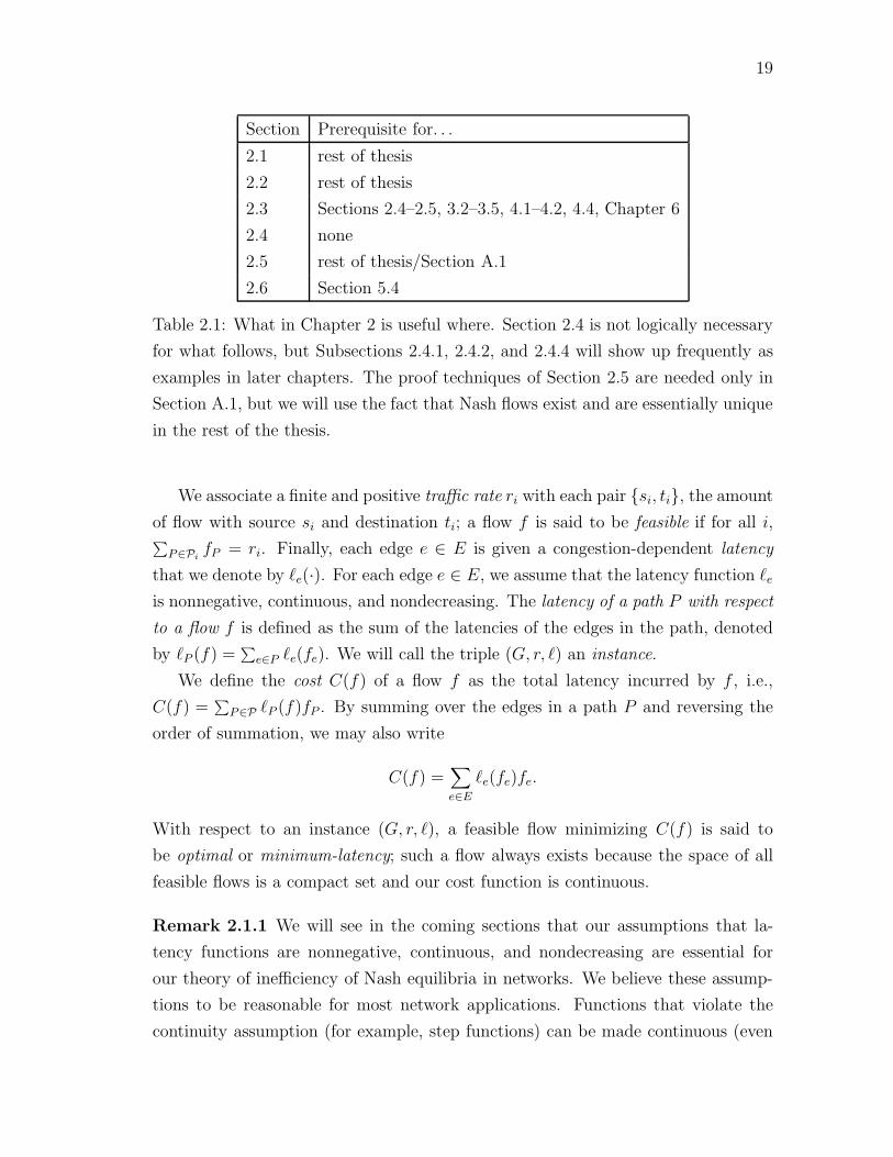
Table 2.1: What in Chapter 2 is useful where. Section 2.4 is not logically necessary

for what follows, but Subsections 2.4.1, 2.4.2, and 2.4.4 will show up frequently as

examples in later chapters. The proof techniques of Section 2.5 are needed only in

Section A.1, but we will use the fact that Nash flows exist and are essentially unique

in the rest of the thesis.

We associate a finite and positive traffic rate ri with each pair si, ti, the amount

of flow with source si and destination ti; a flow f is said to be feasible if for all i,∑P∈Pi

fP = ri. Finally, each edge e ∈ E is given a congestion-dependent latency

that we denote by e(·). For each edge e ∈ E, we assume that the latency function e

is nonnegative, continuous, and nondecreasing. The latency of a path P with respect

to a flow f is defined as the sum of the latencies of the edges in the path, denoted

by P (f) =∑

e∈P e(fe). We will call the triple (G, r, ) an instance.

We define the cost C(f) of a flow f as the total latency incurred by f , i.e.,

C(f) =∑

P∈P P (f)fP . By summing over the edges in a path P and reversing the

order of summation, we may also write

C(f) =∑e∈E

e(fe)fe.

With respect to an instance (G, r, ), a feasible flow minimizing C(f) is said to

be optimal or minimum-latency; such a flow always exists because the space of all

feasible flows is a compact set and our cost function is continuous.

Remark 2.1.1 We will see in the coming sections that our assumptions that la-

tency functions are nonnegative, continuous, and nondecreasing are essential for

our theory of inefficiency of Nash equilibria in networks. We believe these assump-

tions to be reasonable for most network applications. Functions that violate the

continuity assumption (for example, step functions) can be made continuous (even

20

differentiable) with little loss of information. While some researchers have described

scenarios where nonmonotone cost functions are natural1, the applications we have

in mind—routing traffic in computer and road networks—should always satisfy the

required monotonicity condition.

2.2 Flows at Nash Equilibrium

We wish to study flows that represent an equilibrium among many noncooperative

network users—that is, flows that behave “greedily” or “selfishly”, without regard

to the overall cost. We intuitively expect each unit of such a flow (no matter how

small) to travel along the minimum-latency path available to it, where latency is

measured with respect to the rest of the flow; otherwise, this flow would reroute

itself on a path with smaller latency. Following Dafermos and Sparrow [50], we

formalize this idea in the next definition.

Definition 2.2.1 A flow f feasible for instance (G, r, ) is at Nash equilibrium (or

is a Nash flow) if for all i ∈ 1, . . . , k, P1, P2 ∈ Pi with fP1 > 0, and δ ∈ (0, fP1],

we have P1(f) ≤ P2(f), where

fP =

fP − δ if P = P1

fP + δ if P = P2

fP if P /∈ P1, P2.Letting δ tend to 0, continuity and monotonicity of the edge latency functions

give the following useful characterization of a flow at Nash equilibrium, occasionally

called a Wardrop equilibrium [84] or Wardrop’s Principle [175, 176] in the literature,

due to an influential paper of Wardrop [186].

Proposition 2.2.2 A flow f feasible for instance (G, r, ) is at Nash equilibrium if

and only if for every i ∈ 1, . . . , k and P1, P2 ∈ Pi with fP1 > 0, P1(f) ≤ P2(f).

Remark 2.2.3 While Definition 2.2.1 still makes sense without assuming continuity

and monotonicity of the edge latency functions, Proposition 2.2.2 fails if either of

these hypotheses is omitted (the forward direction fails in the absence of continuity

and the reverse direction fails in the absence of monotonicity—see Section B.1).

1For example, Blonski [22] points out that people typically have nonmonotone preferences aboutthe congestion in a restaurant or at a concert, preferring a moderate crowd to total isolation or tobeing packed in like a sardine.

21

Briefly, Proposition 2.2.2 states that, in a flow at Nash equilibrium, all flow

travels on minimum-latency paths. In particular, if f is at Nash equilibrium then

all si-ti flow paths (si-ti paths to which f assigns a positive amount of flow) have

equal latency, say Li(f). We can thus express the cost C(f) of a flow f at Nash

equilibrium in a particularly nice form.

Proposition 2.2.4 If f is a flow at Nash equilibrium for instance (G, r, ), then

C(f) =k∑

i=1

Li(f)ri.

Remark 2.2.5 For the next two sections we will take for granted that Nash flows

exist and are essentially unique; this will be proved in Section 2.5.

Remark 2.2.6 Our definition of a flow at Nash equilibrium corresponds to an

equilibrium in which each network user chooses a single path of the network (a

pure strategy), whereas in classical game theory a Nash equilibrium is defined via

mixed strategies (with players of a game choosing probability distributions over pure

strategies). However, since in our model each network user controls only a negligible

fraction of the overall traffic, these two definitions are essentially equivalent—see [84]

for a rigorous discussion.

2.3 A Characterization of Optimal Flows

We now investigate the properties of an optimal flow—that is, of a flow minimizing

the total latency. Recalling that the cost of a flow f may be expressed C(f) =∑e∈E e(fe)fe, the problem of finding a minimum-latency feasible flow in a network

is a special case of the nonlinear program

Min∑e∈E

ce(fe)

subject to:

(NLP )∑

P∈Pi

fP = ri ∀i ∈ 1, . . . , k

fe =∑

P∈P:e∈P

fP ∀e ∈ E

fP ≥ 0 ∀P ∈ P

where in our problem, ce(fe) = e(fe)fe.

22

For simplicity we have given a formulation with an exponential number of vari-

ables, but it is not difficult to give an equivalent compact formulation (with decision

variables only on edges and explicit node conservation constraints) that requires

only polynomially many variables and constraints.

Next, we characterize the local optima of (NLP ). Roughly, we expect a flow

to be locally optimal if and only if moving flow from one path to another can only

increase the flow’s cost. Put differently, we expect a flow to be locally optimal

when the marginal benefit of decreasing flow along any si-ti flow path is at most

the marginal cost of increasing flow along any other si-ti path. Since the local and

global minima of a convex function on a convex set coincide (see, e.g., [145, Thm

2.3.4]), this condition should be necessary and sufficient for a flow to be globally

optimal whenever the objective function of (NLP ) is convex.2 This is the case

when, for example, for each edge e ∈ E we have ce(fe) = e(fe)fe with a convex

latency function e.

We formalize this characterization of global optima of convex programs of the

form (NLP ) in the next lemma. For a differentiable cost function ce, let c′e denote

the derivative ddx

ce(x) of ce and define c′P (f) by c′P (f) =∑

e∈P c′e(fe). We then have

the following.3

Proposition 2.3.1 ([17, 50]) A flow f is optimal for a convex program of the form

(NLP ) with differentiable cost functions if and only if for every i ∈ 1, . . . , k and

P1, P2 ∈ Pi with fP1 > 0, c′P1(f) ≤ c′P2

(f).

The striking similarity between the characterizations of optimal solutions to a

convex program of the form (NLP ) and of flows at Nash equilibrium was noticed

early on by Beckmann et al. [17], and provides an interpretation of an optimal flow

as a flow at Nash equilibrium with respect to a different set of edge latency functions.

To make this relationship precise, denote the marginal cost of increasing flow on edge

e with differentiable latency function e by ∗e(x) = ddy

(y ·e(y))(x) = e(x)+x ·′e(x).

Propositions 2.2.2 and 2.3.1 then yield the following corollary.

Corollary 2.3.2 ([17, 50]) Let (G, r, ) be an instance with differentiable latency

functions in which x · e(x) is a convex function for each edge e, with marginal cost

2A function f defined on a convex subset S of Rn is convex if f(λx + (1− λ)y) ≤ λf(x) + (1−λ)f(y) for all x, y ∈ S and λ ∈ [0, 1]. Some authors call such functions weakly convex.

3For a formal derivation via the Karush-Kuhn-Tucker Theorem [145], see [17, 50].

23

functions ∗ defined as above. Then a flow f feasible for (G, r, ) is optimal if and

only if it is at Nash equilibrium for the instance (G, r, ∗).

Remark 2.3.3 We will typically denote a minimum-latency flow for an instance by

f ∗. The marginal cost functions are denoted by ∗ since they are “optimal latency

functions” in a sense made precise by Corollary 2.3.2: the optimal flow f ∗ arises as

a flow at Nash equilibrium with respect to latency functions ∗.

Remark 2.3.4 The function ∗e(x) describing the marginal cost of increasing flow on

edge e has one term e(x) capturing the per-unit latency incurred by the additional

flow and a second term x · ′e(x) accounting for the increased congestion experienced

by the flow already using the edge. Essentially, the only difference between an

optimal flow and a flow at Nash equilibrium is that the former accounts for this

“conscientious” second term while the latter disregards it.

The conclusion of Proposition 2.3.1 is false without the convexity hypothesis.

Instances to which Proposition 2.3.1 and Corollary 2.3.2 apply (those with latency

functions satisfying the aforementioned convexity assumption) will play an impor-

tant role in portions of this dissertation (in particular, in Sections 3.3–3.5 and in

Chapter 6), important enough to warrant further terminology.

Definition 2.3.5 A latency function is standard if it is differentiable and if x ·(x)

is convex on [0,∞).

Most but not all latency functions of interest are standard. All differentiable

convex functions are standard, as are some well-behaved nonconvex functions such

as log(1 + x). Differentiable approximations of step functions are the most notable

examples of nonstandard latency functions.

We conclude this section with a final fact about networks with standard latency

functions, useful in Chapter 6: since (NLP ) is a convex program when all edge

latency functions are standard, the optimal flow of such an instance can be found

efficiently.

Fact 2.3.6 If (G, r, ) is an instance with standard latency functions, then the opti-

mal flow for (G, r, ) can be computed in polynomial time (up to an arbitrarily small

additive constant).

This algorithmic task can be accomplished with the ellipsoid method, even when

network latency functions are not described by explicit formulae and are instead

24

given only as oracles [81]. Under additional assumptions on the latency functions

(e.g., that latency functions are sufficiently smooth with efficiently computable first

and second derivatives), standard interior-point techniques (as described in, for ex-

ample, Renegar [152]) can be used. In the special case of an instance with a single

commodity, the problem reduces to that of computing a min-cost flow with re-

spect to a convex separable objective function, a problem for which combinatorial

polynomial-time algorithms are known—see [3, 19, 87] for a survey of the available

techniques.

Remark 2.3.7 The additive error in Fact 2.3.6 is required, as an exact description

of the optimal flow may require irrational numbers.

2.4 Examples

In this section we illustrate the definitions and characterizations of the previous

sections in some concrete networks, and hope to develop the reader’s intuition about

Nash and optimal flows. We first return to the familiar examples of Subsection 1.2

(Pigou’s example and Braess’s Paradox) and then present three more examples that

demonstrate further differences between Nash and optimal flows.

Remark 2.4.1 For simplicity, we have chosen examples in which all traffic shares

the same source and destination. However, we are also interested in (and most of

our results will apply to) networks in which different users have different sources

and destinations.

2.4.1 Pigou’s Example

Recall that, in Pigou’s example of Subsection 1.2.1, we have a network with two

nodes s and t, two parallel edges with latency functions (x) = 1 and (x) = x, and

a traffic rate of 1 (see Figure 2.1(a)). Routing all flow on the bottom link equalizes

the latencies of the two available s-t paths at 1, and thus by Proposition 2.2.2

provides a flow f at Nash equilibrium. By Proposition 2.2.4 (or by inspection), the

cost C(f) of f is 1.

Next, notice that the marginal cost functions of the network are ∗(x) = 1 and

∗(x) = 2x (see Figure 2.1(b)). Routing half of the traffic on each link thus equalizes

25

ts

x

1

(a) Latency Functions

ts

1

2x

(b) Marginal Cost Functions

Figure 2.1: Pigou’s example revisited

s t

w

v

0

1

1 x

x

(a) Latency Functions

s t

w

v

0

2x

1

1

2x

(b) Marginal Cost Functions

Figure 2.2: Braess’s Paradox revisited

the marginal costs of the two s-t paths at 1, and so by Corollary 2.3.2 furnishes a

minimum-latency flow f ∗. The cost of f ∗ is C(f ∗) = 12· 1

2+ 1

2· 1 = 3

4.

2.4.2 Braess’s Paradox

Next we consider the network of Braess’s Paradox (Subsection 1.2.2) after the ad-

dition of the zero-latency edge; see Figure 2.2(a). Setting the traffic rate r to 1, we

see that the flow f that routes all traffic on the path s → v → w → t equalizes the

latency of the three s-t paths at 2, and thus (by Proposition 2.2.2) f is at Nash equi-

librium with C(f) = 2. Switching to marginal cost functions (see Figure 2.2(b)),

we find that the flow f ∗ that routes half the traffic on each of the two two-hop

paths equalizes the marginal costs of the three s-t paths at 2, and is therefore (by

Corollary 2.3.2) optimal. The cost C(f ∗) of f ∗ is 32.

26

ts

1 1

x x

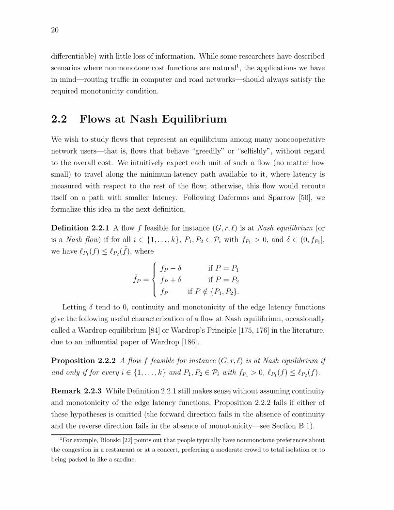
Figure 2.3: The Nash flow may be strictly Pareto-dominated by the optimal flow in

the absence of Braess’s Paradox.

2.4.3 Strict Pareto Suboptimality of Nash without Paradox

In Subsection 1.2.2 we remarked that Braess’s Paradox demonstrates two different

principles. First, all traffic may strictly prefer a coordinated outcome to the flow

at Nash equilibrium4; second, if network users route selfishly, then augmenting a

network with an additional link may strictly increase everyone’s latency. While the

second phenomenon implies the first in the augmented network (by coordinating,

additional links can always be ignored), the converse is not true. Put differently,

there are networks in which the flow at Nash equilibrium is strictly Pareto-dominated

by an optimal flow and yet cannot be improved by the deletion of any number of

network links.

To see this, consider the network shown in Figure 2.3, two copies of the network

of Pigou’s example glued together in series. Setting the traffic rate r to be 1, the

flow f that routes all traffic along the two bottom links equalizes the latency of

all four s-t paths at 2 and is thus at Nash equilibrium. On the other hand, in the

optimal flow f ∗ that routes half of the traffic on the path comprising the top link

of the first subnetwork and the bottom link of second subnetwork and the rest of

the traffic on the path comprising the other two links, all traffic experiences only 32

units of latency. All traffic is thus better off in the flow f ∗ than in the Nash flow f .

Moreover, it is easy to check that the Nash flow does not improve when any subset

of the links of the network is removed.

4In the language of economics, we would say that the Nash flow is strictly Pareto-dominated bythe optimal flow.

27

ts

x

1

p

(a) Latency Functions

ts

1

p (p+1) x

(b) Marginal Cost Functions

Figure 2.4: A nonlinear variant of Pigou’s example

2.4.4 A Nonlinear Variant of Pigou’s Example

In all three of our examples thus far, the Nash flow fails to minimize the total latency

and is a factor of precisely 43

more costly than the optimal flow. This is not entirely

a coincidence, as in the next chapter we will see that no worse ratio is possible in any

multicommodity flow network provided the latency of every edge increases linearly

with the edge congestion (as is the case in the previous three examples). We now

show that this strong hypothesis on the network latency functions is necessary for

such a strong result, and that flows at Nash equilibrium can be arbitrarily more

costly than optimal flows in networks with nonlinear edge latency functions.

Consider the minor modification of Pigou’s example shown in Figure 2.4(a),

where we have replaced the latency function (x) = x by the highly nonlinear one

(x) = xp (for concreteness, think of p as 100 or 1000). With the usual traffic

rate of 1, the Nash flow f is the same as in Pigou’s example; all flow is routed

on the bottom link and the total latency is 1 (for any choice of p). On the other

hand, the discrepancy between the latency functions (in Figure 2.4(a)) and the

marginal cost functions (in Figure 2.4(b)) is much larger; now, the flow f ∗ that

routes (p + 1)−1/p units on the lower link and the remainder on the upper link

equalizes the marginal cost of the two links at 1 and is thus optimal. The cost

C(f ∗) of f ∗ is 1− p · (p+1)−(p+1)/p, which tends to 0 as p → ∞. Thus, if arbitrarily

steep latency functions are allowed (even restricting to polynomials), a flow at Nash

equilibrium can be arbitrarily more costly than an optimal flow. This negative result

motivates our work on bicriteria bounds for Nash flows in networks with arbitrary

latency functions (Section 3.6) and on ensuring that the cost of a selfish solution in

such a network is close to optimal by carefully routing a small fraction of the traffic

centrally (Chapter 6).

28

ts

x

2− ε

(a) Latency Functions

ts

2−

2x

ε

(b) Marginal Cost Functions

Figure 2.5: The optimal flow may sacrifice some traffic to a path with large latency

to minimize the total latency.

2.4.5 The Unfairness of Optimal Flows

In all of our examples thus far, the optimal flow has been superior to the Nash

flow in a very strong sense. Rather than merely achieving a smaller total latency

than a Nash flow, in the previous examples all traffic is at least as well-off in the

optimal flow as in the flow at Nash equilibrium; that is, the optimal flow has Pareto-

dominated the flow at Nash equilibrium. Our next example shows that this will not

always be the case; in general, an optimal flow will sacrifice some traffic to paths

with large latency in order to minimize the total latency experienced by all of the

traffic.

Consider the network of Figure 2.5(a), a small variation on Pigou’s example in

which we replace the latency function (x) = 1 with the latency function (x) = 2−ε

for a very small positive constant ε > 0. As usual, we set the traffic rate r to 1. In

the flow at Nash equilibrium, all traffic is routed on the bottom link and experiences

one unit of latency. In the optimal flow, however, only 1−ε/2 units of flow are routed

on the bottom link—routing the other ε/2 units of traffic on the upper link equalizes

the marginal costs of the two edges at 2−ε. Intuitively, a small fraction of the traffic

is sacrificed to the slow edge in order to (slightly) reduce the congestion experienced

by the overwhelming majority of network users.

The “unfairness” of optimal flows is an unfortunate property. There is good news,

however; for networks in which all traffic shares the same source and destination,

we can quantify this unfairness and prove that it cannot be too large. Since this

issue is somewhat removed from the main themes of this thesis, we defer a further

discussion of it to Section A.3 of Appendix A.

29

2.5 Existence and Uniqueness of Nash Flows

In this section, we exploit the similarity between the characterizations of Nash and

of minimum-latency flows (Propositions 2.2.2 and 2.3.1) to prove the existence and

essential uniqueness of flows at Nash equilibrium. This result is originally due to

Beckmann et al. [17] and was later reproved by Dafermos and Sparrow [50]; we

include a proof for completeness.

Proposition 2.5.1 ([17, 50]) An instance (G, r, ) with continuous, nondecreasing

latency functions admits a flow at Nash equilibrium. Moreover, if f, f are flows at

Nash equilibrium, then e(fe) = e(fe) for each edge e.

Proof. Set he(x) =∫ x0 e(t)dt. By continuity of the latency function e, the function

he is differentiable with nondecreasing derivative e and is therefore convex. Now

consider the convex program

Min∑e∈E

he(fe)

subject to:

(NLP2)∑

P∈Pi

fP = ri ∀i ∈ 1, . . . , k

fe =∑

P∈P:e∈P

fP ∀e ∈ E

fP ≥ 0 ∀P ∈ P

and observe that the optimality conditions of Proposition 2.3.1 are identical to the

characterization of flows at Nash equilibrium in Proposition 2.2.2. The optimal

solutions for (NLP2) are thus precisely the flows at Nash equilibrium for (G, r, ).

Existence of a flow at Nash equilibrium for (G, r, ) then follows from the facts that

(NLP2) has a continuous objective function and a compact feasible region. Next,

suppose f, f are flows at Nash equilibrium for (G, r, ) (and hence global optima for

(NLP2)). By convexity of the objective function of (NLP2), whenever f = f the

objective function must be linear between these two values; otherwise any convex

combination of f, f would be a feasible solution for (NLP2) with smaller objective

function value. Since the objective function is convex separable, he must be linear

between fe and fe for each edge e. By continuity of each latency function e, each e

must be constant between fe and fe. This implies that e(fe) = e(fe) for all e ∈ E,

and the proof is complete.

30

Remark 2.5.2

(a) The proof of Proposition 2.5.1 shows that if each latency function e is strictly

increasing, then the flow fe on edge e in a Nash flow is uniquely determined

for each edge e. Even in this setting there may be several Nash flows, however,

as distinct flows (i.e., distinct functions on the paths P) may induce identical

fe-values on the edges.

(b) In the absence of strictly increasing latency functions, different Nash flows may

place different amounts of flow on the same edge—consider the trivial example

of two nodes and two parallel links endowed with the constant latency function

(x) = 1 (every flow in this network is at Nash equilibrium). Thus in some

sense the uniqueness statement of Proposition 2.5.1 is the strongest possible.

(c) Both the existence and uniqueness conclusions of Proposition 2.5.1 fail if the

hypothesis of continuity is omitted. This fact illustrates a technical distinction

between our traffic routing model (with infinitely many players) and the classi-

cal theory of noncooperative games developed by Nash [130] where, assuming

only finitely many players and mixed strategies but arbitrary cost functions,

a Nash equilibrium always exists. In addition, if latency functions are allowed

to be decreasing or nonmonotone, the uniqueness conclusion fails (see Sec-

tion B.1 for counterexamples). For this reason and others, the assumption of

continuous, nondecreasing network latency functions is crucial for our work.

(d) The proof of Proposition 2.5.1 shows that flows at Nash equilibrium are pre-

cisely the optimal solutions to a related convex program defined over the same

feasible region. Thus, under mild smoothness conditions on the network la-

tency functions, a flow at Nash equilibrium can be computed (up to an ar-

bitrarily small additive constant) in polynomial time; see Fact 2.3.6 and the

comments thereafter for more details.

(e) The reader familiar with noncooperative game theory will recognize the un-

usual ease with which we proved the existence and essential uniqueness of

flows at Nash equilibrium; in general non-zero sum (matrix) games, establish-

ing the existence of Nash equilibria (in mixed strategies) requires recourse to

a nonconstructive fixed-point theorem [130]. That flows at Nash equilibrium

arise as the optimum solutions to a well-behaved optimization problem is both

useful and remarkable, and the recent study of congestion games and potential

31

games by the game theory community can be viewed as an ongoing quest for

broad classes of games that share this property. We will have more to say

about these two classes of games in Section 4.4.

(f) The proof of Proposition 2.5.1 leads to a nontrivial “quick and dirty” upper

bound on the price of anarchy. This bound is easy to apply but does not

in general give the best possible results (unlike the techniques that we will

develop in Chapter 3); for this reason, we defer further discussion of this

bound to Section A.1 in Appendix A.

In much of this thesis, we will be content with the following corollary of Propo-

sition 2.5.1, which states that all flows at Nash equilibrium have the same cost.

Corollary 2.5.3 If f, f are flows at Nash equilibrium for the instance (G, r, ), then

C(f) = C(f).

Proof. The corollary follows directly from Propositions 2.2.4 and 2.5.1.

2.6 Acyclicity of Nash Flows

The goal of this final section is to prove that every instance (G, r, ) admits a Nash

flow without flow cycles (thereby strengthening the existence guarantee of Proposi-

tion 2.5.1). Along the way, we will prove some useful properties about the structure

of minimum-latency paths with respect to a Nash flow.

We begin with an extension of Proposition 2.2.2. While Proposition 2.2.2 char-

acterizes Nash flows as those with all si-ti flow paths having minimum latency (for

each commodity i), the following lemma gives an analogous characterization with

si and ti replaced by an arbitrary pair of vertices.

Proposition 2.6.1 Let f be a flow feasible for the instance (G, r, ). For a vertex

v in G and a commodity i, let di(v) denote the length, with respect to edge lengths

e(fe), of a shortest si-v path in G. Then f is at Nash equilibrium if and only if for

every pair v, w of vertices in G, every commodity i, and every v-w path P :

(a) di(w) − di(v) ≤ ∑e∈P e(fe)

(b) if f ie > 0 for every edge e ∈ P , then di(w) − di(v) =

∑e∈P e(fe).

32

Proof. First suppose f is feasible for (G, r, ) and satisfies the two conditions of the

proposition. For a commodity i, we can take v = si and w = ti and apply properties

(a) and (b) to find that every si-ti flow path of f has minimum latency among all

si-ti paths (namely, di(t)). Since this holds for all commodities, Proposition 2.2.2

implies that f is at Nash equilibrium.

Conversely, suppose f is at Nash equilibrium for (G, r, ). It suffices to prove

that properties (a) and (b) hold when P is a single edge (for a general path, sum

up the inequalities or equalities corresponding to the constituent edges). Then, (a)

follows by definition of di(v) and di(w). To prove (b), consider a commodity i and

an edge e with f ie > 0 and suppose for contradiction that di(w) < di(v) + e(fe).

Let Pe denote an si-ti path containing e with fPe > 0. We may obtain another si-ti

path P ′ via the union of a shortest si-w path and the w-ti path contained in Pe.

Since the latency of the si-w path contained in Pe is at least di(v) + e(fe) > di(w),

we have Pe(f) > P ′(f); by Proposition 2.2.2, this contradicts our assumption that

f is at Nash equilibrium.

It is important to note that the path P in the statement of Proposition 2.6.1

does not need to be a subpath of any flow path of f ; in particular, in property (b)

the flow on different edges of P can be carried by distinct flow paths of f .

By a flow cycle for commodity i of a flow f we mean a collection C of edges

in the underlying graph that form a directed cycle and for which f ie > 0 for all

e ∈ C; we emphasize that flow on different edges may be carried by different si-ti

flow paths. Call a flow f acyclic if it has no flow cycles (for any commodity). We

now prove that every instance admits an acyclic Nash flow, a fact that we believe

to be “folklore”.

Proposition 2.6.2 An instance (G, r, ) admits an acyclic flow at Nash equilibrium.

Proof. An instance (G, r, ) admits a (not necessarily acyclic) Nash flow f by

Proposition 2.5.1. We will first show that flow cycles must comprise only zero-

latency edges, and will then show how to remove such cycles.

For a commodity i, define the si-v distance di(v) of a vertex v with respect to

the flow f as in Proposition 2.6.1. By Proposition 2.6.1 and nonnegativity of edge

latencies, if edge e = (v, w) carries flow then di(w) ≥ di(v). Thus, in a directed cycle

C of flow edges (i.e., of edges e satisfying f ie > 0), all vertices of C have equal di-

values and hence (again by Proposition 2.6.1) all edges of C must have zero latency

with respect to f .

33

We next wish to remove zero-latency flow cycles from f ; this is not entirely trivial

as the flow on different edges of a flow cycle may be carried by different flow paths

(recall f is defined as a function on paths, rather than on edges). We extract a new

feasible flow f from f by running the following procedure for i = 1, 2, . . . , k:

(1) view f i as a function on edges with f ie =

∑P∈Pi:e∈P fP

(2) repeatedly discard flow cycles from f i to obtain an si-ti flow f i (still defined

only on edges) without flow cycles

(3) let f i be an arbitrary path decomposition of f i.

The reader unfamiliar with path decompositions and the discarding of flow cycles

should consult any text on network flow, such as Tarjan [179].

The flow f is acyclic by construction and is feasible for (G, r, ) since only flow

cycles were removed from the feasible flow f ; it remains only to show that f is at

Nash equilibrium. For each edge e, we have either fe = fe or fe < fe with e(fe) = 0

(and hence e(fe) = 0). It follows that e(fe) = e(fe) for every edge e, which in

turn implies that the flows f and f induce identical di-values on the vertices of G

for every commodity i. Appealing to the characterization of Nash flows given in

Proposition 2.6.1, that f is a Nash flow implies that f is, as well.

Part II

Bounding the Price of Anarchy

34

Chapter 3

How Bad is Selfish Routing?

3.1 Introduction

In this chapter we quantify the inefficiency of Nash equilibria in the traffic model

described in the previous two chapters. Recall from our previous examples that

traffic flows at Nash equilibrium (flows in which no network user has an incentive to

reroute its traffic) do not in general minimize the total latency, our measure of social

welfare. In this chapter we study the cost of routing selfishly via the following ques-

tion: given an arbitrary multicommodity flow network with congestion-dependent

edge latencies, what is the worst-possible ratio between the total latency of a flow at

Nash equilibrium and that of the best coordinated outcome—of a flow minimizing

the total latency?

3.1.1 Summary of Results

As discussed in Subsection 1.3.1, this worst-case ratio (“the price of anarchy” [142])

depends crucially on the “steepness” of the network latency functions. We will

present our techniques for computing the price of anarchy in an incremental fash-

ion, with each section considering successively more general classes of edge latency

functions.

The simplest nontrivial networks are those with linear latency functions (where

every edge latency function is of the form (x) = ax+ b for a, b ≥ 0); for this reason

and others, such networks have been studied extensively in the past [71, 72, 143,

144, 175, 176]. Our first result is that in any multicommodity flow network with

linear latency functions, the total latency of a flow at Nash equilibrium is at most

36

37

Description Typical Representative Price of Anarchy

Linear ax + b 43≈ 1.333

Quadratic ax2 + bx + c 3√

33√

3−2≈ 1.626

Cubic ax3 + bx2 + cx + d 4 3√44 3√4−3

≈ 1.896

Polynomials of degree ≤ p∑p

i=0 aixi (p+1) p

√p+1

(p+1) p√

p+1−p= Θ( p

ln p)

M/M/1 Delay Functions (u − x)−1 12

(1 +

√umin

umin−Rmax

)M/G/1 Delay Functions 1

u+ x(1+σ2u2)

2u(u−x)See Section 3.5

Table 3.1: The price of anarchy for common classes of edge latency functions. Poly-

nomial coefficients are assumed nonnegative. The parameters u and σ are the ex-

pectation and standard deviation of the associated queue service rate distribution.

Rmax denotes the maximum allowable amount of network traffic, and umin denotes

the minimum allowable edge service rate (or capacity).

43

times that of a minimum-latency flow (with a matching lower bound provided by

any of the first three examples of Section 2.4). We also demonstrate how this result

provides a quantitative limit on the extent to which counterintuitive phenomena

can occur in certain physical systems, such as the strings and springs example of

Figure 1.3.

The assumption of linear latency functions is quite restrictive; we next demon-

strate how to enhance the techniques developed for networks with linear latency

functions to compute the price of anarchy with respect to an (almost) arbitrary

class of latency functions. We apply this generalization to additional classes of

latency functions that are well-studied in the networking and queueing theory liter-

ature; in particular, all of the results shown in Table 3.1 follow directly from these

techniques.

These methods also show that the underlying network topology plays no role in

the determination of the price of anarchy. Specifically, we show that under weak

hypotheses on the class of allowable latency functions1, the worst-case ratio between

the total latency of a flow at Nash equilibrium and that of a minimum-latency flow

in any multicommodity flow network is achieved by a single-commodity instance on

1For example, it suffices for the class to satisfy a mild convexity assumption, to be closed undermultiplication by positive scalars, and to possess some latency function that is positive whenevaluated with zero congestion. Almost all classes of latency functions previously considered inthe literature meet the required hypotheses.

38

a set of parallel links. In the special case of a class of latency functions that includes

all of the constant functions, we prove that a network with only two parallel links

suffices to achieve the worst-possible ratio. Informally, these results imply that

the inefficiency inherent in a flow at Nash equilibrium stems from the inability of

selfish users to discern which of two competing routes is superior and not from the

topological complexity arising from the diverse intersections of many paths belonging

to different commodities.

Finally, we employ a bicriteria approach to bound the inefficiency of Nash flows

in networks with arbitrary latency functions (where our previous work shows that

Nash flows may be arbitrarily more costly than optimal flows). We show that in a

multicommodity flow network with latency functions assumed only to be continuous

and nondecreasing, the total latency incurred by traffic at Nash equilibrium is at

most that of a minimum-latency flow forced to route twice as much traffic between

each source-destination pair. We show that this result also has the following alter-

native interpretation: in lieu of centralized control, the price of routing selfishly can

be offset by a moderate increase in link speed (which for queueing delay functions

can be effected by a moderate increase in the network capacity).

3.1.2 Related Work

Traffic Equilibria

Unregulated traffic has been modeled as network flow with all flow paths between

a given source-destination pair having minimum latency since the 1950’s [17, 186]

(though as mentioned in Chapter 1, Pigou [148] and Knight [99] informally discussed

a similar model thirty years earlier). Wardrop [186] formulated the notions of a flow

at Nash equilibrium and of a minimum-latency flow, and suggested that these were

the two types of traffic flows deserving special study. Beckmann et al. [17], observing

that a flow at Nash equilibrium is an optimal solution to a related convex program

(see Section 2.3), gave existence and uniqueness results for traffic equilibria. Dafer-

mos and Sparrow [50] reproved many of the results of [17] and were also interested

in computing flows at Nash equilibrium efficiently; in particular, they proposed two

iterative algorithms for computing Nash flows and proved convergence results for

certain networks.

Since these early works, the traffic model studied in this dissertation has been

generalized in many different directions. In the transportation science literature,

39

this model has been generalized to allow for the latency of an edge to depend on the

entire traffic pattern (rather than merely on the flow using that edge), to include

different types (or “modes”) of traffic, to allow elastic (rather than fixed) traffic

rates, and so on; research on these more general models have focused on establishing

existence and uniqueness of traffic equilibria [1, 26, 32, 45, 46, 47, 66, 67, 68, 84, 85,

102, 129, 173, 192], on designing algorithms to compute an equilibrium [1, 11, 18,

45, 46, 65, 66, 67, 68, 69, 78, 115, 118, 129, 134, 135, 187, 192], and on sensitivity

analysis [45, 49, 83, 190]. For an introduction to this literature, we recommend

the survey of Florian and Hearn [68] and the book of Sheffi [169]. More recently,

Nesterov [131] (see also Nesterov and De Palma [132]) has proposed an interesting

alternative to (rather than a generalization of) the traffic model considered in this

thesis.

In the networking literature, many recent papers alter the model considered here

by relaxing the assumption that every network user controls a negligible fraction of

the overall traffic (as will we in Sections 4.2 and 4.3); rather, a finite number of

users each control a positive amount of flow. Most of these papers allow players

to split their flow among several routes but disallow randomization, and then give

necessary and sufficient conditions (on the network topology, the amount of flow that

users control, and on the edge latency functions) for the existence and uniqueness

of (pure-strategy) Nash equilibria [4, 8, 25, 59, 138] and for convergence to a Nash

equilibrium under natural models of user behavior [5, 138]. Some of these results

have been extended to networks in which users cannot split flow and must instead

route all of their traffic on a single path [117].

Finally, the game theory community has generalized the traffic model studied

here to broad classes of games that need not take place in a network. This literature

(which we will review in Section 4.4, when we study a related class of games) aims

to identify games that enjoy many of the desirable properties possessed by traffic

equilibria, such as existence of Nash equilibria in pure strategies, rather than to

model any specific type of application.

The Price of Anarchy

In contrast to the previous work on traffic equilibria, we are interested in quanti-

fying the difference in social welfare between equilibrium and optimal traffic flows.

The idea of bounding the inefficiency of Nash equilibria was first proposed by Kout-

soupias and Papadimitriou [108] for the following simple load-balancing model. A

40

finite number of users share a collection of parallel links, and each user chooses a

probability distribution on the set of links (specifying the probability that the user

will route all of its flow on a given link). Each user wishes to minimize the expected

congestion it will experience, while the global objective is to minimize the expected

load on the most congested edge; the worst-case Nash equilibrium is then compared

to a globally optimal choice of distributions. Koutsoupias and Papadimitriou [108]

obtained a tight analysis of this worst-case ratio (which they call the coordination

ratio) in two-node, two-link networks and partial results for two-node networks with

three or more parallel links; tight results were subsequently found for parallel net-

works with any number of links by Mavronicolas and Spirakis [122] (for a special

case) and by Czumaj and Vocking [44] (for the general case). More recently, the

original model of [108] has been generalized by Czumaj et al. [43] (for example, to

include more general objective functions), who also prove a variety of facts about

the coordination ratio in this more general model.

3.1.3 Organization

In Sections 3.2–3.5 we present our methods for computing the price of anarchy;

these sections should be read in order. In Section 3.2 we study networks with linear

latency functions and prove that the price of anarchy for such networks is 43. We

also demonstrate the connection between networks with linear latency functions and

the networks of strings and springs advertised in Subsection 1.3.1. In Sections 3.3

and 3.4 we generalize these techniques to show that the price of anarchy is inde-

pendent of the network topology, and in Section 3.5 we show how this fact permits

computation of the price of anarchy with respect to an arbitrary class of latency

functions. Section 3.5 also illustrates our techniques by computing the price of

anarchy for important classes of latency functions not considered earlier.

Finally, in Section 3.6 we prove that a Nash flow in a network with arbitrary

latency functions costs no more than an optimal flow forced to route twice as much

traffic. This section does not depend on earlier results of this chapter and can be

read immediately following Section 2.2.

41

3.2 The Price of Anarchy with Linear Latency

Functions

In this section, we consider the scenario where the latency of each edge e is linear in

the edge congestion—that is, where for each edge e ∈ E, e(x) = aex + be for some

ae, be ≥ 0. This is the setting in which Braess’s paradox was originally discovered [28,

128], and several subsequent papers focused entirely on this model [71, 72, 143, 144,

175, 176]. In addition, linear latency functions are important for other applications:

we will see later in this section that the mechanical networks of strings and springs

described in Subsection 1.3.1 can be modeled as traffic networks with linear latency

functions, and Friedman [74] shows how linear latency functions naturally arise in a

simple model of selfish users transferring files over a network employing a congestion

control protocol (such as TCP).

We have already seen in Subsections 2.4.1–2.4.3 three examples with linear la-

tency functions for which the ratio of the cost of a flow at Nash equilibrium and

the cost of an optimal flow is 43. Our main result for this section (Theorem 3.2.6)

is a matching upper bound for networks with linear latency functions. The proof

techniques of this section will also form the basis for our subsequent work bounding

the price of anarchy for networks with nonlinear latency functions.

To make these statements precise, we require some additional notation. For an

instance (G, r, ) admitting an optimal flow f ∗ and a flow at Nash equilibrium f , we

denote the ratio C(f)C(f∗)

by ρ = ρ(G, r, ); this ratio is well defined by Corollary 2.5.3.

We begin by noting that the propositions of Section 2.3 have particularly simple

and useful forms in the special case of networks with linear latency functions. First,

the total latency C(f) of a flow f is given by C(f) =∑

e aef2e +befe; since ae ≥ 0 for

all e, the nonlinear program (NLP ) of Section 2.3 is a convex (quadratic) program

and thus Proposition 2.3.1 characterizes its optimal solutions. Also, in the notation

of Section 2.3, if the latency function e of edge e is e(x) = aex + be, then the

marginal cost function ∗e of e is simply ∗e(x) = 2aex + be. For convenience, we

summarize this discussion together with specialized versions of Propositions 2.2.2

and 2.3.1 in the following lemma.

Lemma 3.2.1 Let (G, r, ) be an instance with edge latency functions e(x) = aex+

be for each e ∈ E. Then,

(a) a feasible flow f is at Nash equilibrium for (G, r, ) if and only if for each

42

commodity i and P, P ′ ∈ Pi with fP > 0,

∑e∈P

aefe + be ≤∑e∈P ′

aefe + be

(b) a feasible flow f ∗ is optimal for (G, r, ) if and only if for each commodity i

and P, P ′ ∈ Pi with f ∗P > 0,

∑e∈P

2aef∗e + be ≤

∑e∈P ′

2aef∗e + be.

As an aside, we note that Lemma 3.2.1 immediately gives a simple proof of the

following nontrivial result regarding networks in which the latency of each edge is

proportional to its congestion; this result is implicit in the work of Dafermos and

Sparrow [50], and other properties of this special case have been investigated in the

context of electrical networks [24, 39].

Corollary 3.2.2 Let G be a network in which each edge latency function e is of

the form e(x) = aex. Then for any rate vector r, a flow feasible for (G, r, ) is

optimal if and only if it is at Nash equilibrium.

Proof. A feasible flow for such an instance satisfies the conditions of Lemma 3.2.1(a)

if and only if it satisfies the conditions of Lemma 3.2.1(b).

A second corollary of Lemma 3.2.1 will play a crucial role in our proof of the

main theorem of this section.

Lemma 3.2.3 Suppose (G, r, ) has linear latency functions and f is a flow at Nash

equilibrium. Then,

(a) the flow f/2 is optimal for (G, r/2, )

(b) the marginal cost of increasing the flow on a path P with respect to f/2 equals

the latency of P with respect to f .

Proof. For part (a), simply note that if f satisfies the conditions of Lemma 3.2.1(a)

for (G, r, ), then f/2 satisfies the conditions of Lemma 3.2.1(b) for (G, r/2, ). For

the second part, recall that if edge e has latency function e(x) = aex + be then e

has marginal cost function ∗e(x) = 2aex + be. Thus, ∗e(fe/2) = e(fe) for each edge

e and hence ∗P (f/2) = P (f) for each path P .

43

An outline of the proof of the main theorem is as follows. It will be useful to

think about creating an optimal flow for the instance (G, r, ) via a two-step process:

in the first step, a flow optimal for the instance (G, r/2, ) is sent through G (which

from Lemma 3.2.3(a) we know to be simply half of a Nash flow for (G, r, )), and in

the second step this flow is augmented to one optimal for (G, r, ). It is important

to note that this augmentation may increase or decrease the amount of flow on any

given edge—e.g., in Braess’s Paradox (Figure 2.2) the Nash flow f (and hence the

flow f/2) makes use of the zero-latency edge (v, w) while the optimal flow eschews it.

We will show that the first flow has cost at least 14C(f) and that the augmentation

has cost at least 12C(f), where f is some flow at Nash equilibrium.

We will see in the proof of Theorem 3.2.6 that the first lower bound follows

easily from Lemma 3.2.3(a), but the second (for the cost of the augmentation, given

that the first flow has already been routed) requires more work, and in particular

the following lemma. Intuitively, the lemma simply claims that the per-unit cost

of increasing the amount of flow through a network is at least the marginal cost of

increasing flow on any path with respect to the current optimal flow.

Lemma 3.2.4 Suppose (G, r, ) is an instance with linear latency functions for

which f ∗ is an optimal flow. Let L∗i (f

∗) be the minimum marginal cost of increasing

flow on an si-ti path with respect to f ∗. Then for any δ > 0, a feasible flow for the

instance (G, (1 + δ)r, ) has cost at least

C(f ∗) + δk∑

i=1

L∗i (f

∗)ri.

Proof. A heuristic proof of this lemma is as follows. Since the marginal cost of

increasing flow on any si-ti path with respect to f ∗ is at least L∗i (f

∗), routing δri

additional units of flow from si to ti should cost at least δL∗i (f

∗)ri. Summing over all

commodities i should then yield the lemma. This argument provides good intuition

for why the lemma is true, but is not sufficient because not all feasible flows for

(G, (1+ δ)r, ) are obtainable from f ∗ by simply routing additional flow through the

network.

To prove the lemma, fix δ > 0 and suppose f is feasible for (G, (1 + δ)r, ). In

general fe may be larger or smaller than f ∗e . For any edge e ∈ E, convexity of the

function x · e(x) = aex2 + bex implies that

e(fe)fe ≥ e(f∗e )f ∗

e + (fe − f ∗e )∗e(f

∗e ).

44

In essence, this inequality states that estimating the cost of changing the flow value

on edge e from f ∗e to fe by (fe −f ∗

e )∗e(f∗) (i.e., by the marginal cost of flow increase

at f ∗e times the size of the perturbation) only underestimates the actual cost of an

increase (when fe > f ∗e ) and overestimates the actual benefit of a decrease (when

fe < f ∗e ). We may thus derive

C(f) =∑e∈E

e(fe)fe

≥ ∑e∈E

e(f∗e )f ∗

e +∑e∈E

(fe − f ∗e )∗e(f

∗e )

= C(f ∗) +k∑

i=1

∑P∈Pi

∗P (f ∗)(fP − f ∗P ).

Since we have ∗P (f ∗) ≥ L∗i (f

∗) for each i and each P ∈ Pi and equality holding

whenever f ∗P > 0 (see Lemma 3.2.1(b)), we obtain

C(f) ≥ C(f ∗) +k∑

i=1

L∗i (f

∗)∑

P∈Pi

(fP − f ∗P )

= C(f ∗) + δk∑

i=1

L∗i (f

∗)ri,

completing the proof.

Remark 3.2.5 Lemma 3.2.4 and its proof remain valid in much more general set-

tings; all that is required is convexity of the function x · e(x) for each edge e (i.e.,

that each latency function is standard—recall Definition 2.3.5).

We are now prepared to prove the main theorem.

Theorem 3.2.6 If (G, r, ) has linear latency functions, then ρ(G, r, ) ≤ 43.

Proof. Let f be a flow at Nash equilibrium for (G, r, ). Let Li(f) be the la-

tency of an si-ti flow path, so that C(f) =∑

i Li(f)ri (see Proposition 2.2.4). By

Lemma 3.2.3(a), f/2 is an optimal flow for the instance (G, r/2, ). Moreover, by

Lemma 3.2.3(b), L∗i (f/2) = Li(f) for each i—in words, marginal costs with respect

to f/2 and latencies with respect to f coincide. This establishes the necessary con-

nection between the cost of augmenting f/2 to a flow feasible for (G, r, ) and the

cost of a flow at Nash equilibrium.

Taking δ = 1 in Lemma 3.2.4, we find that the cost of any flow f ∗ feasible for

(G, r, ) satisfies

C(f ∗) ≥ C(f/2) +k∑

i=1

L∗i (f/2)

ri

2

45

= C(f/2) +1

2

k∑i=1

Li(f)ri

= C(f/2) +1

2C(f).

Finally, it’s easy to lower bound the cost of f/2:

C(f/2) =∑e

1

4aef

2e +

1

2befe

≥ 1

4

∑e

aef2e + befe

=1

4C(f)

and thus C(f ∗) ≥ 34C(f).

We note that the analysis of this section can easily be extended to prove that in

an instance (G, r, ) where for some p, e(x) = aexp + be (with ae, be ≥ 0) for each

edge e, ρ(G, r, ) ≤ (1 − p · (p + 1)−(p+1)/p)−1 = Θ( pln p

). The nonlinear variant of

Pigou’s example (Subsection 2.4.4) shows that this result is tight. In Section 3.5 we

will see that this upper bound holds more generally for instances with polynomial

latency functions with nonnegative coefficients and any number of terms with degree

at most p.

Consequences for Strings and Springs

We now return to the mechanical networks of strings and springs discovered by Co-

hen and Horowitz [36] and discussed in Subsection 1.3.1 and Figure 1.3. Viewing the

support as a source and the suspended weight as a destination, with each string and

spring as an edge, the equilibrium position of the mechanical device can be modeled

as a flow at Nash equilibrium in a traffic network G, with force corresponding to

flow and support-weight distance corresponding to the common latency of every

source-destination flow path. Strings (as perfectly inelastic objects) are modeled as

links with constant latency functions while (perfectly elastic) springs correspond to

links with latency functions that include a term of the form ax. Severing a string

or spring corresponds to deleting an edge from a traffic network; thus any realizable

equilibrium of the mechanical network (after possibly destroying some of its con-

stituent parts) corresponds to a Nash equilibrium in a subgraph of the corresponding

traffic network G.

46

Although Theorem 3.2.6 is concerned with the total latency of flows (a concept

with no natural analogue in our mechanical networks), we can use the result in the

following way. By Theorem 3.2.6, every traffic flow in G (and in particular every

flow at Nash equilibrium in a subgraph of G) has total latency at least 34

times that

of a Nash flow f in G. By Proposition 2.2.4, it follows that if the common latency

of every flow path of f is L and f ∗ is a flow at Nash equilibrium in a subgraph of

G, then the common latency of every flow path of f ∗ is at least 34L. Reinterpreting

this result for networks of strings and springs, we obtain the following corollary of

Theorem 3.2.6.

Corollary 3.2.7 In any network of strings and springs carrying a single weight with

support-weight distance D, the support-weight distance after severing an arbitrary

collection of strings and springs is at least 34D.

Cohen and Horowitz [36] also showed, by an analogous construction, that re-

moving a diode from a two-terminal electrical network of resistors and diodes can

decrease the voltage drop from source to ground—thus removing a conducting link

can increase the network conductivity. By the same arguments as above, Theo-

rem 3.2.6 implies that the voltage drop from source to ground in such an electrical

network after removing any number of resistors and diodes is at least 34

times the

voltage drop in the original network.

3.3 The Price of Anarchy with Standard Latency

Functions

The goal of this section is to provide an upper bound on the worst-case ratio be-

tween the cost of a Nash flow and of an optimal flow for instances with nonlinear

latency functions. As we have seen in the nonlinear variant of Pigou’s example

(Subsection 2.4.4), the price of anarchy depends crucially on how “steep” the allow-

able latency functions can be, and one may therefore ask whether any meaningful

upper bound is possible for networks with arbitrary latency functions. The answer

is affirmative, provided that the upper bound is a function of the class of allowable

latency functions.

To state the main result of this section precisely, recall that ρ(G, r, ) denotes the

ratio between the cost of a Nash and of an optimal flow for instance (G, r, ). We will

associate a real number α(L) ≥ 1 to each class L of allowable edge latency functions

47

that quantifies the “steepness” of the latency functions in L, and will then prove

that for any instance (G, r, ) with latency functions in the class L, ρ(G, r, ) ≤ α(L).

In Section 3.4 we will provide a matching lower bound, by exhibiting (for any class

L) instances with latency functions in L and ρ-value arbitrarily close to α(L).

3.3.1 The Anarchy Value

Our first task is to find a definition that captures how “steep” a given class of al-

lowable latency functions is. A first attempt attempt might involve the first several

derivatives of the latency functions; for example, we might hope to prove that if the

first few derivatives of all allowable latency functions are everywhere bounded by

some universal constant, then the price of anarchy is constant. However, any in-

stance (G, r, ) with latency functions of class Ck (latency functions that are k times

continuously differentiable) can be “scaled down” to an instance (G, r, 1M

) in which

the first k derivatives of all edge latency functions are as small as desired (by taking

M sufficiently large). Moreover, ρ(G, r, 1M

) = ρ(G, r, ) since a feasible flow is opti-

mal (respectively, Nash) for (G, r, 1M

) if and only if is optimal (respectively, Nash)

for (G, r, ). Thus, networks with latency functions with (any number of) bounded

derivatives are not “better-behaved” than networks with polynomial latency func-

tions; and from the nonlinear variant of Pigou’s example (Subsection 2.4.4), we

already know that networks with polynomial latency functions and no upper bound

on the allowable degree are not well-behaved at all.

Before giving our definition capturing how “steep” a given class of allowable la-

tency functions is (which, admittedly, is not immediately intuitive), we will consider

a motivating example. It will be convenient to apply Corollary 2.3.2 to compute the

optimal flow in this example; for this reason and others that will become clear later

in this section, we restrict ourselves to networks with standard latency functions (see

Definition 2.3.5). Since the focus of this section is on classes of allowable latency

functions, we make another definition.

Definition 3.3.1 A class L of latency functions is standard if L contains a nonzero

function and if each ∈ L is standard.

We now introduce the motivating example. Suppose we are given a standard

class L of allowable latency functions, and wish to construct a network in which the

Nash flow incurs much more latency than the optimal flow. A natural idea is to

mimic the bad example of Subsection 2.4.4 as best we can, given that L is the class

48

of latency functions that we are allowed to work with. For simplicity, assume that

the constant function 1(x) = 1 lies in L. Then, we can consider the usual two-node,

two-link network, assign the first link the latency function 1 and the second link

the “steepest” latency function that we can find. More formally, suppose 2 ∈ Lis assigned to the second link where 2 satisfies 2(0) < 1 and 2(x) > 1 for x

sufficiently large. Choosing r > 0 to satisfy 2(r) = 1, we find that a Nash flow

with traffic rate r routes all of its flow on the second edge for a total latency of

r. Using Corollary 2.3.2 and letting λ ∈ (0, 1) satisfy ∗2(λr) = 1, we find that the

optimal flow routes λr units of flow on the second link and (1 − λ)r units of flow

on the first link, for a total latency of λr2(λr) + (1− λ)r. Letting µ ∈ [0, 1] denote

2(λr), the ratio between the total latency of the Nash flow and of the optimal flow

is [λµ + (1 − λ)]−1. Taking into account that this argument can be used with 1

replaced by any constant function, and that 2 ∈ L was chosen arbitrarily, we arrive

at the following definition.

Definition 3.3.2 Let be a nonzero standard latency function. The anarchy value

α() of is

α() = supr>0 : (r)>0

[λµ + (1 − λ)]−1

where λ ∈ (0, 1) satisfies ∗(λr) = (r) and µ ∈ [0, 1] is defined by µ = (λr)/(r).

That the scalar λ ∈ (0, 1) exists follows from the Intermediate Value Theorem and

the fact that ∗(0) = (0) ≤ (r) ≤ ∗(r). In most cases of interest λ will be uniquely

determined by and r; otherwise, our assumption that is standard ensures that

the anarchy value is well defined (i.e., that [λµ + (1 − λ)]−1 is independent of the

choice of λ satisfying ∗(λr) = (r)).

The anarchy value of a latency function should be interpreted as the worst

possible ratio between the cost of a Nash flow and of an optimal flow in a two-node,

two-link network where one edge possesses latency function and the other possesses

a constant latency function; the worst-case is taken over choices of the constant and

of the traffic rate.

Since we are interested only in the “steepest” latency functions of a class, the

next definition should be unsurprising.

Definition 3.3.3 The anarchy value α(L) of a standard class L of latency functions

is

α(L) = sup0=∈L

α().

49

Remark 3.3.4

(a) The anarchy value of a class lies in [1,∞] and need not be finite.

(b) The anarchy value seems a fearsome expression to compute analytically, but we

will see in Section 3.5 that it can typically be worked out in cases of practical

interest.

(c) There are also simpler definitions of “steepness” that provide nontrivial but

suboptimal upper bounds on the price of anarchy; see Sections A.1 and A.2 of

Appendix A.

We have already argued informally that if L is a standard class of latency func-

tions containing the constant functions, then there are instances I on a network with

two nodes and two links and latency functions in L with ratio ρ arbitrarily close to

α(L). On the other hand, there is no reason a priori to expect the anarchy value to

have any connection to instances defined on more general networks (even to those

defined on parallel networks with more than two links). The central result of this

section is that, under very weak conditions on the class of allowable latency func-

tions, α(L) upper bounds ρ(G, r, ) for any instance (G, r, ) with latency functions

in L (with an arbitrary network topology and an arbitrary number of commodities).

3.3.2 Proof Approach

We next discuss our proof approach. At the highest level, the proof of this section

is inspired by that of the last section, which shows that the price of anarchy for

networks with linear latency functions is precisely 43. Let us recapitulate the three

main steps of that proof. First, we used the characterizations of Nash and optimal

flows (via Corollary 2.3.2) to show that if f is a flow at Nash equilibrium for an

instance (G, r, ) with linear latency functions, then the scaled-down flow f/2 is

optimal for the instance (G, r/2, ). Second, we lower bounded the cost of f/2 in

terms of the cost of f ; this was not difficult since the scaled-down flow f/2 was a

“significant fraction” of f . Finally, we lower bounded the cost of augmenting the

flow f/2 to a flow optimal for (G, r, ) in terms of the cost of f . This was the most

difficult part of the proof; roughly, we leveraged the connection between Nash and

optimal flows given in Corollary 2.3.2 to show that the marginal cost of routing new

flow with respect to f/2 is high, and thus augmenting the flow f/2 to a flow feasible

for the full set of traffic rates r is costly.

50

A direct attempt at adapting the three-step approach of the previous section

to more general latency functions fails immediately. In particular, for nonlinear

latency functions (even for quadratic latency functions), there is no constant c for

which a scaled-down version f/c of a Nash flow f is optimal for the reduced traffic

rates r/c. Thus, it is not at all clear how to exploit our characterizations of Nash

and optimal flows to relate their respective costs. To circumvent this problem, we

view the proof approach of the previous section in the following more general way:

chop up an optimal flow into two “pieces” (in the linear latency case, f/2 and an

augmentation from f/2 to a flow feasible for rates r) such that each piece can be

lower-bounded in terms of the cost of a Nash flow. Guided by a desire to define the

second piece of the optimal flow as an augmentation of the first and to lower bound

its cost by means of marginal cost functions (as in the linear latency case), we will

define the first piece in a way that ensures that any augmentation with respect to

it has large marginal cost. Unfortunately, this requires scaling down a Nash flow f

by different factors on different edges, thereby producing an object which is not a

flow (it is a more general object that need not obey conservation constraints, which

we call a pseudoflow). While this does not significantly complicate the lower bound

for the cost of the scaled-down pseudoflow (it is a “significant fraction” of the Nash

flow, as before), a more careful analysis is now required to lower bound the cost of

an augmentation from the scaled-down pseudoflow to a flow feasible for the original

instance (as we are augmenting with respect to an object more complicated than

simply a flow at reduced traffic rates).

3.3.3 Proof of Upper Bound

We now turn toward making these ideas precise. We first define what we mean by a

“scaled-down pseudoflow”. The idea is to scale down the amount of Nash flow on a

single edge until the value of the marginal cost function equals the original latency

incurred by the Nash flow on that edge (this original latency is then our definition

of “large marginal cost”). Formally, if f is a flow at Nash equilibrium, our scaled-

down pseudoflow will be defined by λefee∈E where λe satisfies ∗e(λefe) = e(fe)

(as in Definition 3.3.2). As discussed following Definition 3.3.2, these scaling factors

always exist but need not be unique; our analysis must work with an arbitrary choice

of scaling factors.

The next lemma formalizes the notion of “breaking up the optimal flow into two

pieces”. Again, the idea is to express the cost of the optimal flow as one term that

51

is a scaled-down version of a Nash flow, and a second term that corresponds to an

augmentation with respect to large marginal costs.

Lemma 3.3.5 Let f ∗ and f be optimal and Nash flows, respectively, for instance

(G, r, ) with standard latency functions. For an edge e, let λe ∈ (0, 1) be a solution

to ∗e(λefe) = e(fe). Then,

C(f ∗) ≥∑e

[e(λefe)λefe + (f ∗e − λefe)e(fe)] .

Proof. Since each edge latency function e is standard, each marginal cost function

∗e is nondecreasing. For an edge e, we may thus write

e(f∗e )f ∗

e = e(λefe)λefe +∫ f∗

e

λefe

∗e(x)dx

≥ e(λefe)λefe + (f ∗e − λefe)

∗e(λefe)

= e(λefe)λefe + (f ∗e − λefe)e(fe)

with the final equality holding by the definition of λe. Summing over all edges proves

the lemma.

Note that neither the statement nor the proof of Lemma 3.3.5 assumes that the

expression f ∗e − λefe is nonnegative for all edges e; as in the previous section, the

augmentation from the pseudoflow defined by λefee∈E to a flow f ∗ optimal for the

original instance may increase or decrease the amount of flow on an edge.

To lower bound the right-hand side of Lemma 3.3.5, we require two more easy

lemmas. The next lemma simply rephrases Definitions 3.3.2 and 3.3.3.

Lemma 3.3.6 Let L be a standard class of latency functions with anarchy value

α(L). For ∈ L and f > 0, let λ ∈ (0, 1) satisfy ∗(λf) = (f) and define µ by

µ = (λf)/(f) (if (f) = 0, put µ = 1). Then λµ + (1 − λ) ≥ 1α(L)

.

Our final lemma states that if f is a Nash flow for (G, r, ), then f is a min-cost

flow (in the classical sense of network flow theory [179]) with respect to the cost

vector e(fe).

Lemma 3.3.7 Let f be at Nash equilibrium and f ∗ feasible for instance (G, r, ).

Then, ∑e

e(fe)fe ≤∑e

e(fe)f∗e .

52

Proof. Let Li(f) denote the common latency of every si-ti flow path of f , so that

∑e

e(fe)fe = C(f) =k∑

i=1

Li(f)ri

by Proposition 2.2.2. Since f is at Nash equilibrium, P (f) ≥ Li(f) for every si-ti

path P ; we may thus write

∑e

e(fe)f∗e =

k∑i=1

∑P∈Pi

P (f)f ∗P ≥

k∑i=1

Li(f)ri,

proving the lemma.

With all of the preliminaries now in place, we state and prove the main result

of this section: the anarchy value of a standard class L of latency functions upper

bounds the ratio ρ for any instance with latency functions in L.2

Theorem 3.3.8 Let L be a standard class of latency functions with anarchy value

α(L). Let (G, r, ) denote an instance with latency functions drawn from L. Then

ρ(G, r, ) ≤ α(L).

Proof. By Lemma 3.3.5 we have

C(f ∗) ≥ ∑e

[e(λefe)λefe + (f ∗e − λefe)e(fe)]

=∑e

[µeλefe + (1 − λe)fe + (f ∗e − fe)]e(fe)

=∑e

[µeλefe + (1 − λe)fe]e(fe) +∑e

[f ∗e − fe]e(fe)

where λe ∈ (0, 1) is chosen (arbitrarily) to satisfy ∗e(λefe) = e(fe) and where

µe ∈ [0, 1] is defined by µe = e(λefe)/e(fe) (if e(fe) = 0, put µe = 1). The second

sum is nonnegative by Lemma 3.3.7, so we may derive

C(f ∗) ≥∑e

[µeλefe + (1 − λe)fe]e(fe);

applying Lemma 3.3.6 we obtain

C(f ∗) ≥ ∑e

[µeλe + (1 − λe)]e(fe)fe

≥ 1

α(L)

∑e

e(fe)fe

=C(f)

α(L)

and the theorem is proved.

2We are indebted to Amir Ronen for substantially simplifying our original proof of this theorem.

53

3.4 The Price of Anarchy is Independent of the

Network Topology

With Theorem 3.3.8 in hand, it is now a relatively easy matter to prove that the price

of anarchy is independent of the network topology. In Subsection 3.4.1 we prove that,

with respect to a standard class of allowable edge latency functions that contains

the constant functions, the worst possible value of ρ(G, r, ) for a multicommodity

instance (G, r, ) is realized (up to an arbitrarily small additive factor) by a single-

commodity instance on a two-node, two-link network. In Subsection 3.4.2, we prove

that under significantly weaker conditions on the class of allowable latency functions,

the worst-case value of ρ(G, r, ) is achieved (again, up to an arbitrarily small factor)

by a single-commodity instance on a network of parallel links.

3.4.1 Lower Bounds in Two-Link Networks

We begin by formalizing an argument of the previous section; the following lemma

is essentially a restatement of Definitions 3.3.2 and 3.3.3.

Lemma 3.4.1 Let G2 denote the graph with one source vertex, one destination ver-

tex, and two edges directed from source to destination. Let L denote a standard class

of latency functions containing the constant functions, with anarchy value α(L). If

I2 denotes the set of all instances with underlying network G2 and latency functions

in L, then

sup(G2,r,)∈I2

ρ(G2, r, ) ≥ α(L).

Proof. We will assume that α(L) is finite, and will leave the straightforward

modifications necessary for the α(L) = +∞ case to the interested reader.

For any ε > 0, choose a nonzero latency function 1 ∈ L, a positive number

r > 0 with 1(r) > 0, and a scalar λ ∈ (0, 1) satisfying ∗1(λr) = 1(r) so that

[λµ+(1−λ)]−1 ≥ α(L)− ε, where µ = 1(λr)/1(r). Let 2 ∈ L denote the constant

function that is everywhere equal to 1(r). Define an instance on G2 with latency

functions 1 and 2 and traffic rate r. The total latency incurred by the Nash flow

is 1(r)r, while that of the optimal flow is 1(r)r[λµ + (1− λ)]; hence the ρ-value of

this instance is at least α(L) − ε. Since ε > 0 was arbitrary, the lemma follows.

Combining Theorem 3.3.8 and Lemma 3.4.1, we find that the price of anarchy

with respect to a standard class of latency functions containing the constant func-

54

tions is independent of the class of allowable network topologies (thereby generalizing

Theorem 3.2.6 and the matching lower bound of Pigou’s example).

Theorem 3.4.2 Let G2 denote the graph with one source vertex, one destination

vertex, and two edges directed from source to destination. Let L be a standard class

of latency functions containing the constant functions. If I denotes the set of all

instances with latency functions in L and I2 ⊆ I the instances with underlying

network G2, then

sup(G2,r,)∈I2

ρ(G2, r, ) = α(L) = sup(G,r,)∈I

ρ(G, r, ).

3.4.2 Lower Bounds in Networks of Parallel Links

We now relax the assumption that the class of allowable latency functions con-

tains all of the constant functions, and assume instead the following much weaker

condition: for any positive real number a, there is a latency function satisfying

(0) = a. We call such a class of latency functions diverse. For any class of latency

functions that is closed under multiplication by positive scalars3, diversity merely

asserts that some latency function is positive when evaluated at 0. Under these

weaker hypotheses, we have the following.

Lemma 3.4.3 Let Gm denote the graph with one source vertex, one destination

vertex, and m edges directed from source to destination. Let L be a standard and

diverse class of latency functions with anarchy value α(L). If Im denotes the set of

all instances with underlying network Gm and latency functions in L, then

sup(G,r,)∈∪mIm

ρ(G, r, ) ≥ α(L).

Proof. We again assume for simplicity that α(L) is finite. For any ε > 0, choose

a nonzero latency function 1 ∈ L, a positive number r > 0 with 1(r) > 0, and a

scalar λ ∈ (0, 1) satisfying ∗1(λr) = 1(r) so that [λµ + (1 − λ)]−1 ≥ α(L) − ε/2,

where µ = 1(λr)/1(r). Since L is diverse, there is a function 2 ∈ L satisfying

2(0) = 1(r). The main idea of the proof is to use many links, all with latency

function 2, to approximately “simulate” a single link with the constant latency

function everywhere equal to 1(r).

3Since a scalar multiplication of the latency functions can be effected simply by changing theunits in which we measure latency, we expect most classes of interest to satisfy this property.

55

Let m be so large that 2((1−λ)rm−1

) ≤ 1(r) + δ, where δ is a sufficiently small

positive number (depending on ε) to be chosen later; existence of the integer m

follows from continuity of 2 at 0. Define an instance on Gm with traffic rate r,

latency function 1 on one link, and latency function 2 on the other m − 1 links.

The total latency incurred by the Nash flow is 1(r)r, as all flow is routed on the

link with latency function 1. The flow that routes λr units of flow on the link with

latency function 1 at a cost of λrµ1(r) and (1− λ)r/(m− 1) units of flow on each

of the other m − 1 links has total latency at most 1(r)r[λµ + (1 − λ) + 1−λ1(r)

δ], by

choice of m. Choosing δ sufficiently small, we obtain an instance with ρ-value at

least α(L) − ε. Since ε > 0 was arbitrary, the lemma follows.

Theorem 3.3.8 and Lemma 3.4.3 together imply the main result of this section.

Theorem 3.4.4 Let Gm denote the graph with one source vertex, one destination

vertex, and m edges directed from source to destination. Let L be a standard and

diverse class of latency functions. If I denotes the set of all instances with latency

functions in L and Im ⊆ I the instances with underlying network Gm, then

sup(G,r,)∈∪mIm

ρ(G, r, ) = α(L) = sup(G,r,)∈I

ρ(G, r, ).

Remark 3.4.5 The conclusion of the theorem is false with ∪mIm replaced by I2

(for a counterexample, take L = (x) = x ∪ (x) = a(1 + x) : a > 0). The

conclusion of the theorem is also false when the class of allowable latency functions

need not be diverse (for a counterexample, let L = (x) = 1 + x).

Remark 3.4.6 That the price of anarchy is independent of the network topology

is a remarkable fact; to better appreciate this, we will foreshadow some forthcoming

results. In Chapter 4 we will generalize the traffic model studied in this chapter in

several different directions, and we will often see that general network topologies are

more poorly-behaved than networks of parallel links. In Chapter 5 we will study

Braess’s Paradox and generalizations of it, and will discover that the severity of

the paradox grows with the network size and cannot occur in networks of parallel

links. Finally, in Chapter 6 we will generalize the traffic model studied here to

accommodate a different equilibrium concept, Stackelberg equilibria, and will prove

that the inefficiency of such equilibria can be strictly larger in general network

topologies than in networks of parallel links.

56

3.5 Computing the Price of Anarchy

In this section, we leverage the results of Sections 3.3 and 3.4 to show that com-

puting the price of anarchy with respect to an (almost) arbitrary standard class of

latency functions reduces to computing the anarchy value of the class, even when the

diversity condition of Theorem 3.4.4 fails (as in the important case of M/M/1 delay

functions with some minimum allowable queue service rate). This provides a gen-

eral reduction from a combinatorial problem (finding a worst-case instance among

all possible multicommodity flow instances) to a simpler analytical one (finding the

“steepest” latency function in a given class). Subsection 3.5.1 describes this method,

and Subsection 3.5.2 computes the price of anarchy for several important function

classes.

3.5.1 More Techniques for Computing the Price of Anarchy

In the previous section, we saw that the price of anarchy with respect to a standard

and diverse class of latency functions is precisely the anarchy value of the class

(Theorem 3.4.4). In this subsection we will show that this fact remains true under

even weaker hypotheses. From a computational perspective, this result has the

following interpretation: to compute the price of anarchy with respect to an (almost)

arbitrary standard class of latency functions L, it suffices to compute the worst-

possible ratio between the cost of a Nash and of an optimal flow in a two-node,

two-link network where one link possesses a constant latency function and the other

link possesses a latency function of the form ν for ∈ L and a positive scalar ν > 0

(even though L need not contain ν or any constant functions).

The first step of this reduction is the following lemma, which implies that we

can always assume that our class of latency functions is closed under multiplication

by positive scalars.

Lemma 3.5.1 Let L be a standard class of latency functions, and define L as the

closure of L under multiplication by positive scalars (so L = ν : ∈ L, ν > 0).Let I denote the set of instances with latency functions in L, and I the set of

instances with latency functions in L. Then,

sup(G,r,)∈I

ρ(G, r, ) = sup(G,r,)∈I

ρ(G, r, ).

57

Proof. The left-hand side trivially lower bounds the right-hand side since L ⊇ Land hence I ⊇ I. For the reverse inequality, we will show that for any instance

(G, r, ) ∈ I and any ε > 0, there is an instance (G, r, ) ∈ I satisfying ρ(G, r, ) ≥ρ(G, r, ) − ε. Fix an instance (G, r, ) ∈ I and ε > 0, and for an edge e of G write

e = νee for νe > 0 and e ∈ L. The ratio ρ is a continuous function of each scalar νe

(holding the network G and the traffic rate vector r fixed), and we may thus replace

each νe by a sufficiently close positive rational number ηe to obtain a new instance

with ρ-value at least ρ(G, r, )−ε. Clearing denominators, we may assume that each

scalar ηe is a positive integer (multiplying all latency functions of an instance by a

common positive number does not affect its ρ-value). Finally, replacing each edge e

with a directed path of ηe edges, each endowed with latency function e, we obtain

a network with latency functions in L and with ρ-value at least ρ(G, r, ) − ε.

The following observation will also be useful.

Lemma 3.5.2 Let L be a standard class of latency functions, and define L as the

closure of L under multiplication by positive scalars. Then L and L have equal

anarchy value.

Proof. Simply note that the functions and ν (for 0 = ∈ L and ν > 0) have

equal anarchy value.

Lemmas 3.5.1 and 3.5.2 yield the following theorem, which reduces computing

the price of anarchy (the combinatorial problem of finding a worst-possible multi-

commodity flow instance) to computing the anarchy value (the simpler analytical

problem of determining the worst behavior exhibited by any function in a given

class).

Theorem 3.5.3 Let L be a standard class of latency functions containing a function

satisfying (0) > 0, with anarchy value α(L). If I denotes the set of instances with

latency functions in L, then

sup(G,r,)∈I

ρ(G, r, ) = α(L).

Proof. Since L is standard and contains a function that is positive at 0, the class

L = ν : ∈ L, ν > 0 is standard and diverse. By Theorem 3.4.4, we have

sup(G,r,)∈I

ρ(G, r, ) = α(L)

58

where I denotes the set of instances with latency functions in L. Applying Lem-

mas 3.5.1 and 3.5.2, we obtain the desired equality.

Remark 3.5.4 The conclusion of Theorem 3.5.3 fails if the hypothesis that some

function is positive with zero congestion is omitted (recall Corollary 3.2.2 and con-

sider the counterexample class L = ax : a > 0). We do not know if the as-

sumption that the function class is standard can be omitted. We leave open the

problem of computing the price of anarchy for classes of latency functions that fail

to satisfy these two hypotheses, though it is not clear if such function classes have

any practical import.

3.5.2 Applications

We are finally prepared to put our techniques to use in computing the price of

anarchy for some concrete function classes. We give only three illustrative examples;

it will be obvious that many other function classes can be treated in a similar way.

Polynomial Latency Functions

For a positive integer p, let Lp denote the set of latency functions that are polyno-

mials with nonnegative coefficients and degree at most p. As a first showcase for our

machinery, we next compute the price of anarchy with respect to latency functions

Lp.

Proposition 3.5.5 If Ip is the set of instances with latency functions in Lp, then

sup(G,r,)∈Ip

ρ(G, r, ) = [1 − p · (p + 1)−(p+1)/p]−1 = Θ(

p

ln p

).

Proof. Since Lp is standard and contains the constant functions, Theorem 3.4.2

implies that the price of anarchy is simply the anarchy value of Lp. We claim

that it suffices to compute the anarchy value of the smaller function class consist-

ing of functions of Lp comprising only one term, namely Lp ≡ axi : a ≥ 0, i ∈0, 1, 2, . . . , p. This claim is valid because an instance (G, r, ) with latency func-

tions in Lp can be transformed into an equivalent instance with latency functions

in Lp by replacing an edge e of G with latency function e(x) =∑p

i=0 aixi by a di-

rected path of p+1 edges, with the ith edge of the path possessing latency function

59

e,i(x) = aixi.4

We next compute the anarchy value α() of an arbitrary nonzero function (x) =

axi of Lp (recall Definition 3.3.2). If i = 0 then α() = 1; otherwise, ∗ is strictly

increasing and the scalar λ is uniquely determined by the choice of r. In this case,

for r > 0 we have λ = (i+1)−1/i, hence µ = λi = (i+1)−1, hence [λµ+(1−λ)]−1 =

[(i + 1)−(i+1)/i + (1− (i + 1)−1/i)]−1 = [1− i · (i + 1)−(i+1)/i]−1. Since this expression

is independent of r > 0, we obtain α() = [1 − i · (i + 1)−(i+1)/i]−1. This expression

is independent of a and is increasing in i on [0, p] (as shown by a simple derivative

test), so the functions of Lp with largest anarchy value are those of the form axp for

a > 0; hence, α(Lp) = α(Lp) = [1 − p · (p + 1)−(p+1)/p]−1.

Remark 3.5.6 A sharp lower bound on the left-hand side of Proposition 3.5.5

is provided by the nonlinear variant of Pigou’s example (Subsection 2.4.4); the

content of the proposition is that no worse example is possible, even in arbitrary

multicommodity flow networks.

Delay Functions of M/M/1 Queues

Latency functions of the form (x) = (u − x)−1 arise as the (expected) delay func-

tion of an M/M/1 queue5 with service rate (or capacity) u [80], and for this reason

have been extensively studied in the networking literature [20, 105, 106, 113, 138].

These latency functions do not directly fit into our framework, since they are de-

fined only on the set [0, u), rather than on all of [0,∞). Nevertheless, only minor

generalizations of our results are needed to compute the price of anarchy in this

setting.

We will fix two parameters, the largest allowable sum of all traffic rates Rmax

and the smallest allowable edge capacity umin. We will assume that Rmax < umin;

while it may seem unreasonable to assume that any edge of the network has the

capacity to carry all of the demand, our computations below will show that, in the

absence of further assumptions, the price of anarchy is +∞ if the sum of traffic

rates can be arbitrarily close to (or greater than) the smallest edge capacity. Under

this assumption, the restricted domains of the latency functions pose no difficulty;

4This maneuver illustrates a general principle: if L is the cone generated by a (possibly infinite)standard class of latency functions S (i.e., L is all finite affine combinations of functions in S),then α(L) = α(S).

5By M/M/1, we mean a single queue with Poisson arrivals and exponentially distributed servicetimes [80].

60

every feasible flow routes at most Rmax units of flow on every edge and hence has a

well-defined cost.

Let L denote the set of latency functions (x) = (u − x)−1 : u ≥ uminand, for the purposes of this example only, redefine the anarchy value α() of a

latency function to be α() = supr : 0<r≤Rmax[λµ+(1−λ)]−1, where λ is the unique

scalar satisfying ∗(λr) = (r) and µ = (λr)/(r). The key difference between this

definition and the original definition of anarchy value (Definition 3.3.2) is that the

range of traffic rates we consider is restricted to lie in (0, Rmax] rather than (0,∞);

this ensures that the equations defining λ and µ make sense.

Next, it is straightforward to check that Theorem 3.3.8 and hence Theorem 3.5.3

remain valid with our new definition of anarchy value, provided we only care about

the worst-possible value of ρ achieved by instances whose sum of all traffic rates is at

most Rmax. Since the class L satisfies both hypotheses of Theorem 3.5.3, computing

the price of anarchy with respect to L for instances with sum of all traffic rates at

most Rmax reduces to computing the anarchy value of L.

Proposition 3.5.7 If I is the set of instances with latency functions in L and sum

of all traffic rates at most Rmax, then

sup(G,r,)∈I

ρ(G, r, ) =1

2

(1 +

√umin

umin − Rmax

).

Proof. The previous discussion implies that we need only check that α(L) =

[1 +√

umin/(umin − Rmax)]/2. We begin by computing the anarchy value of an

arbitrary function in L, say (x) = (u − x)−1 for u ≥ umin. The marginal cost

function ∗ is given by ddx

(x(u − x)−1) and hence

∗(x) =u

(u − x)2.

Now fix r ∈ (0, Rmax]; λ is defined to solve the equation ∗(λr) = (r) and hence

satisfiesu

(u − λr)2=

1

u − r.

Solving, we obtain λ = (u −√

u(u − r))/r. Next,

µ =(λr)

(r)=

u − r

u − λr=

u − r

u − (u −√u√

u − r)=

√u − r√

u.

61

It remains to compute [λµ + (1 − λ)]−1:

[λµ + (1 − λ)]−1 =

[u −√

u√

u − r

r

√u − r√

u+ 1 − u −√

u√

u − r

r

]−1

=

[2u

√u − r − 2u

√u + 2r

√u

r√

u

]−1

=1

2

r√u√

u − r − (u − r)·√

u√

u − r + (u − r)√u√

u − r + (u − r)

=1

2

r[√

u√

u − r + (u − r)]

u(u − r) − (u − r)2

=1

2

√u√

u − r + (u − r)

u − r

=1

2

(1 +

√u

u − r

).

Since this expression is increasing in r, it follows that

α() =1

2

(1 +

√u

u − Rmax

).

Since the anarchy value is decreasing in the edge capacity, we have

α(L) =1

2

(1 +

√umin

umin − Rmax

),

as claimed.

Remark 3.5.8

(1) We note that the above class L is not diverse (since (0) ≤ 1umin

for all ∈ L);

indeed, the worst-possible value of the ratio ρ need not be achieved on a set

of parallel links for this class of latency functions (cf. Theorem 3.4.4).6 Thus,

the extensions provided in Subsection 3.5.1 are crucial in this application.

(2) The anarchy value of L and hence the worst possible value of ρ go to +∞as Rmax → umin; fulfilling a previous promise, this shows that the hypothesis

that Rmax is bounded away from umin is necessary for the price of anarchy for

networks with M/M/1 delay functions to be finite.

6However, the proof of Lemma 3.5.1 shows that subdivisions of parallel networks suffice toachieve the worst-case bound.

62

Delay Functions of M/G/1 Queues

As a final example, we extend the preceding analysis to queues that need not have

exponentially distributed service times—that is, to M/G/1 delay functions (we re-

tain our assumptions of a single queue and Poisson arrivals). Our solution will not

be as clean as in the M/M/1 case, but will demonstrate that our techniques for

computing the price of anarchy remain useful even for relatively complex classes of

allowable latency functions.

Recall that if a queue service distribution (specifying the number of customers

served in a time step) has expectation µ and standard deviation σ (both of which

we assume to be finite), then the expected waiting time under Poisson arrivals with

rate λ is1

µ+

λ(1 + σ2µ2)

2µ(µ − λ);

see [80] or [94] for a derivation. To rephrase this formula in our usual notation, we

view the parameter µ as the edge capacity u and the Poisson rate λ as the amount

of traffic assigned to an edge; we are then interested in latency functions of the

following form:

(x) =1

u+

x(1 + σ2u2)

2u(u− x).

As in the M/M/1 case, to achieve an interesting result we will need to assume a

minimum allowable capacity umin and a maximum allowable sum of all traffic rates

Rmax < umin.

The anarchy value of such a function can be computed by the same method as

for M/M/1 case (though the calculations are more tedious). It turns out that the

anarchy value of a latency function with the above formula is

α() =

(1 +

√u

u − Rmax

)2u + Rmax(σ

2u2 − 1)

4u + (u + Rmax −√

u(u − Rmax))(σ2u2 − 1).

Applying Theorem 3.5.3, we obtain the following proposition.

Proposition 3.5.9 Let L be a non-empty collection of M/G/1 delay functions with

expected service rate at least umin. Then, the price of anarchy for instances with

latency functions in L and sum of all traffic rates at most Rmax < umin is precisely

sup∈L

(1 +

√u

u − Rmax

)2u + Rmax(σ

2 u

2 − 1)

4u + (u + Rmax −√

u(u − Rmax))(σ2 u

2 − 1)

where u and σ denote the expectation and standard deviation of the service rate

distribution associated with .

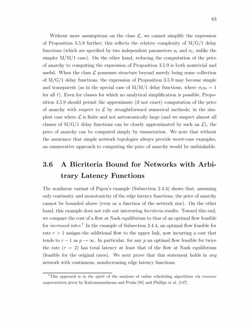
63

Without more assumptions on the class L, we cannot simplify the expression

of Proposition 3.5.9 further; this reflects the relative complexity of M/G/1 delay

functions (which are specified by two independent parameters u and σ, unlike the

simpler M/M/1 case). On the other hand, reducing the computation of the price

of anarchy to computing the expression of Proposition 3.5.9 is both nontrivial and

useful. When the class L possesses structure beyond merely being some collection

of M/G/1 delay functions, the expression of Proposition 3.5.9 may become simple

and transparent (as in the special case of M/M/1 delay functions, where σu = 1

for all ). Even for classes for which no analytical simplification is possible, Propo-

sition 3.5.9 should permit the approximate (if not exact) computation of the price

of anarchy with respect to L by straightforward numerical methods; in the sim-

plest case where L is finite and not astronomically large (and we suspect almost all

classes of M/G/1 delay functions can be closely approximated by such an L), the

price of anarchy can be computed simply by enumeration. We note that without

the assurance that simple network topologies always provide worst-case examples,

an enumerative approach to computing the price of anarchy would be unthinkable.

3.6 A Bicriteria Bound for Networks with Arbi-

trary Latency Functions

The nonlinear variant of Pigou’s example (Subsection 2.4.4) shows that, assuming

only continuity and monotonicity of the edge latency functions, the price of anarchy

cannot be bounded above (even as a function of the network size). On the other

hand, this example does not rule out interesting bicriteria results. Toward this end,

we compare the cost of a flow at Nash equilibrium to that of an optimal flow feasible

for increased rates.7 In the example of Subsection 2.4.4, an optimal flow feasible for

rate r > 1 assigns the additional flow to the upper link, now incurring a cost that

tends to r − 1 as p → ∞. In particular, for any p an optimal flow feasible for twice

the rate (r = 2) has total latency at least that of the flow at Nash equilibrium

(feasible for the original rates). We next prove that this statement holds in any

network with continuous, nondecreasing edge latency functions.

7This approach is in the spirit of the analyses of online scheduling algorithms via resourceaugmentation given by Kalyanasundaram and Pruhs [91] and Phillips et al. [147].

64

fe

flow

feel ( )

late

ncy

(a) Graph of latency function e

and its value at flow value fe

fe

flow

feel ( )

late

ncy

(b) Graph of latency function e

Figure 3.1: Construction in the proof of Theorem 3.6.1 of modified latency function

e given original latency function e and Nash flow value fe. Solid lines denote

graphs of functions.

Theorem 3.6.1 If f is a flow at Nash equilibrium for (G, r, ) and f ∗ is feasible

for (G, 2r, ), then C(f) ≤ C(f ∗).

Proof. Suppose f, f ∗ satisfy the hypotheses of the theorem. For i = 1, . . . , k,

let Li(f) be the latency of an si-ti flow path of f , so that C(f) =∑

i Li(f)ri

(see Proposition 2.2.4). We seek a set of latency functions that on one hand

approximates the original ones (in the sense that the cost of a flow with respect to

latency functions is close to its original cost) and, on the other hand, allows us to

easily lower bound the cost (with respect to ) of any feasible flow. With this goal

in mind, we define new latency functions as follows:

e(x) =

e(fe) if x ≤ fe

e(x) if x ≥ fe.

Figure 3.1 illustrates this construction.

First we compare the cost of the flow f ∗ under the new latency functions to

its original cost C(f ∗). For any edge e, e(x)− e(x) is zero for x ≥ fe and bounded

above by e(fe) for x < fe, so x(e(x) − e(x)) ≤ e(fe)fe for all x ≥ 0. Notice

that the left-hand side (the discrepancy between xe(x) and xe(x)) is maximized

when x is slightly smaller than fe and when e(x) = 0; in this case, the value of

the left-hand side is essentially the area of the rectangle enclosed by dashed lines in

Figure 3.1(a). The difference between the new cost (with respect to ) and the old

65

cost (with respect to ) can now be bounded as follows:∑e

e(f∗e )f ∗

e − C(f ∗) =∑e∈E

f ∗e (e(f

∗e ) − e(f

∗e ))

≤ ∑e∈E

e(fe)fe

= C(f).

In other words, evaluating f ∗ with latency functions (rather than ) increases its

cost by at most an additive C(f) factor.

On the other hand, if f0 denotes the zero flow in G, then by construction P (f0) ≥Li(f) for any path P ∈ Pi. Since e is nondecreasing for each edge e, it follows that

P (f ∗) ≥ Li(f) for each path P ∈ Pi. Thus, the cost of f ∗ with respect to can be

bounded below in the following manner:∑P

P (f ∗)f ∗P ≥ ∑

i

∑P∈Pi

Li(f)f ∗P

=∑

i

2Li(f)ri

= 2C(f).

Combining these two results we obtain the theorem:

C(f ∗) ≥ ∑P

P (f ∗)f ∗P − C(f)

≥ 2C(f) − C(f)

= C(f).

The same proof also shows the following more general result.

Theorem 3.6.2 If f is a flow at Nash equilibrium for (G, r, ) and f ∗ is feasible

for (G, (1 + ξ)r, ), then C(f) ≤ 1ξC(f ∗).

Remark 3.6.3 Referring back to the network of Subsection 2.4.4 (the network with

two nodes and two edges with latency functions (x) = 1 and (x) = xp), we see

that Theorem 3.6.2 is essentially tight for all values of ξ. More precisely, by taking

p sufficiently large we can obtain an instance admitting an optimal flow feasible for

a traffic rate arbitrarily close to (1 + ξ) with cost strictly less than ξ (recall the cost

of the flow at Nash equilibrium for the original rate r = 1 is 1) and an optimal flow

feasible for rate 1 + ξ with cost arbitrarily close to ξ.

66

Theorem 3.6.1 has a natural interpretation for networks with the M/M/1 delay

functions mentioned in the previous section. To see this, we first note that comparing

a Nash flow to an optimal flow forced to route more traffic is the same as comparing a

Nash flow with “faster” latency functions to an optimal flow in the original network.

Formally, we have the following corollary of Theorem 3.6.1.

Corollary 3.6.4 Let (G, r, ) be an instance and define the modified latency func-

tion e by e(x) = 12e(

x2) for each edge e. If f is a flow at Nash equilibrium for

(G, r, ) and f ∗ is feasible for (G, r, ), then the cost of f (with respect to latency

functions ) is at most the cost of f ∗ (with respect to latency functions ).

Proof. Let f be a Nash flow for (G, r/2, ) and f ∗ a flow feasible for (G, r, ); by

Theorem 3.6.1,∑

e e(fe)fe ≤ ∑e e(f

∗e )f ∗

e . Now consider the flow f = 2f , viewed

as a feasible flow for (G, r, ). Since e(fe) = 12e(fe) for each edge e and f is a Nash

flow for (G, r, ), f is a Nash flow for (G, r, ); moreover,

∑e

e(fe)fe =∑e

(1

2e(fe))(2fe) =

∑e

e(fe)fe.

We have shown that∑

e e(fe)fe ≤ ∑e e(f

∗e )f ∗

e with f at Nash equilibrium for

(G, r, ); the corollary now follows from the essential uniqueness of Nash flows (Corol-

lary 2.5.3).

Now consider the special case of an instance (G, r, ) in which all latency functions

are the delay functions of M/M/1 queues, and thus for each edge e we have e(x) =

(ue − x)−1 on [0, ue) for some edge capacity ue. Assume for simplicity that every

flow f feasible for (G, r, ) satisfies fe < ue for each edge e (e.g., by insisting that the

minimum edge capacity is larger than the sum of all traffic rates), so that we can

ignore the restricted domains of the latency functions. Here, if e(x) = 1/(ue − x)

then e(x) = 1/2(ue − x/2) = 1/(2ue − x). Thus in a network with M/M/1 delay

functions, Corollary 3.6.4 offers the following advice: to match the performance of a

centrally controlled network with selfish routing, simply double the capacity of every

edge.

Remark 3.6.5 We made the strong assumption that every feasible flow f satisfies

fe < ue for each edge e for simplicity. We can alternatively define the latency

of an edge with an M/M/1 delay function and capacity u to be +∞ on [u,∞);

arithmetic with +∞ is defined in the usual way. Some care must be taken with this

67

approach, however, as the essential uniqueness of Nash flows (Proposition 2.5.1 and

Corollary 2.5.3) fails when edge latencies can take on +∞ as a value; in particular,

some but not all Nash flows may have infinite cost. The guarantee of Theorem 3.6.1

also fails for networks in which Nash flows may have infinite cost. What remains

true is this: doubling the capacity of a network with M/M/1 delay functions is

guaranteed to offset the cost of selfish routing, assuming only that all Nash flows

in the augmented network possess finite cost. This significantly weakens our earlier

assumption that all feasible flows have finite cost in the original network.

Chapter 4

Extensions to Other Models

In Chapter 3 we studied the price of anarchy in the network model put forth in

Chapter 2. In this chapter we show how this work can be extended both to more

realistic models of network routing and to a broader class of games. We do not

endeavor to generalize all of the results of the previous chapter to the greatest

possible extent; we merely wish to point out that our techniques are not entirely

model-specific, and to indicate some directions in which they are readily extended.

The extensions presented in the first three sections of this chapter are motivated

by some of the deficiencies of the traffic model defined in Chapter 2. First, net-

work users can often only evaluate path latency approximately, rather than exactly.

Section 4.1 extends the notion of a flow at Nash equilibrium and Theorems 3.2.6

and 3.6.1 to this setting. Second, our basic model represents an idealized scenario

with infinitely many users each controlling a negligible fraction of the overall traffic,

while in reality we encounter a finite number of network users, each controlling a

strictly positive amount of traffic. In Section 4.2 we prove an analogue of Theo-

rem 3.6.1 for the case of finitely many network users, provided each user can route

its flow fractionally over any number of paths. In Section 4.3 we show that such an

assumption is essentially necessary, in that no bicriteria bound analogous to The-

orem 3.6.1 holds when there are only finitely many network users, each of whom

must route its flow on a single path; however, a version of Theorem 3.6.1 does hold

if network users do not control too much flow and the edge latency functions are not

too steep. In the last section (Section 4.4), we show how all of the results of Chap-

ter 3 can be extended to a broad class of games (that need not involve a network)

previously studied in the game theory literature.

68

69

4.1 Flows at Approximate Nash Equilibrium

It is often unreasonable to expect network users to be able to evaluate the latency

of different paths with arbitrary precision. We next investigate the sensitivity of our

results to this assumption. We suppose that a network user can only distinguish

between paths that differ significantly in their latency (say by more than a (1 + ε)

factor for some ε > 0). Our definition of a flow at ε-approximate Nash equilibrium

is then an obvious modification of Definition 2.2.1:

Definition 4.1.1 A flow f feasible for instance (G, r, ) is at ε-approximate Nash

equilibrium if for all i ∈ 1, . . . , k, P1, P2 ∈ Pi, and δ ∈ (0, fP1], we have P1(f) ≤(1 + ε)P2(f), where

fP =

fP − δ if P = P1

fP + δ if P = P2

fP if P /∈ P1, P2.The analogue of Proposition 2.2.2 is then:

Lemma 4.1.2 A flow f is at ε-approximate Nash equilibrium if and only if for

every i ∈ 1, . . . , k and P1, P2 ∈ Pi with fP1 > 0, P1(f) ≤ (1 + ε)P2(f).

The next theorem provides an analogue of Theorem 3.6.1 for flows at ε-approx-

imate Nash equilibrium.

Theorem 4.1.3 If f is at ε-approximate Nash equilibrium with ε < 1 for (G, r, )

and f ∗ is feasible for (G, 2r, ), then C(f) ≤ 1+ε1−ε

C(f ∗).

Proof. Suppose f, f ∗ satisfy the hypotheses of the theorem. For i = 1, . . . , k, let

Li(f) be the minimum latency of any si-ti path (with respect to f); since f is at ε-

approximate Nash equilibrium, every si-ti flow path has latency at most (1+ε)Li(f)

and hence C(f) ≤ (1 + ε)∑

i Li(f)ri.

As in the proof of Theorem 3.6.1, we define a new set of latency functions by

e(x) =

e(fe) if x ≤ fe

e(x) if x ≥ fe.

As before, the cost of a flow with respect to exceeds its cost with respect to by

at most an additive factor of C(f).

70

Letting f0 denote the zero flow in G, we have P (f0) ≥ Li(f) for any path P ∈ Pi.

Since e is nondecreasing for each edge e, it follows that P (f ∗) ≥ Li(f) for each

path P ∈ Pi. This allows us to bound the cost of f ∗ with respect to from below:∑P

P (f ∗)f ∗P ≥ ∑

i

∑P∈Pi

Li(f)f ∗P

=∑

i

2Li(f)ri

≥ 2

1 + εC(f).

To conclude, we derive

C(f ∗) ≥ ∑P

P (f ∗)f ∗P − C(f)

≥ 2

1 + εC(f) − C(f)

=1 − ε

1 + εC(f).

Remark 4.1.4 A simple example in a network similar to that of Braess’s Paradox

(Figure 1.2(b)) shows that the factor of 1+ε1−ε

cannot be improved (see Section B.2).

However, it is not difficult to improve this factor to 1 + ε in networks of parallel

links (see Section B.2); this provides a counterpoint to our work in Sections 3.3–3.4

showing that worst-case examples for the price of anarchy for flows at exact Nash

equilibrium always occur in networks of parallel links.

Further extensions of the theorems of Chapter 3 to the current setting are possi-

ble. As an example, we sketch an approximate version of Theorem 3.2.6 for networks

with linear latency functions. As in Section 3.2, the idea is to start with a flow f at

ε-approximate Nash equilibrium and consider the scaled-down flow f/2. The claim

C(f/2) ≥ 14C(f) holds as in Section 3.2, but now f/2 is only approximately optimal

for (G, r/2, ); because of this, proving that an augmentation from f/2 to a flow

feasible for (G, r, ) is costly will require a bit of care.

Next, let Li(f) denote the minimum latency of any si-ti path with respect to f .

The following are true:

(1) C(f) ≤ (1 + ε)∑k

i=1 Li(f)ri.

(2) If P is an si-ti path, then the marginal cost of P with respect to f/2 is at

least Li(f).

71

(3) If P is an si-ti flow path of f , then the marginal cost of P with respect to f/2

is at most (1 + ε)Li(f).

Now consider augmenting f/2 to a flow f ∗ optimal for (G, r, ). As in Lemmas 3.2.4

and 3.3.5, convexity of the objective function C(·) with linear (or more generally,

standard) latency functions allows us to lower bound the cost of this augmentation

on each edge by the change in flow value times the marginal cost with respect to f/2.

At worst, this augmentation will remove ri/2 units of flow between each commodity

i at a marginal benefit of (1 + ε)Li(f) per flow unit and will add ri units of flow at

a marginal cost of Li(f) per flow unit. This argument gives

C(f ∗) ≥ 1

4C(f) − (1 + ε)

k∑i=1

Li(f)ri

2+

k∑i=1

Li(f)ri

=1

4C(f) +

(1 − ε

2

) k∑i=1

Li(f)ri

≥ C(f)

(1

4+

1 − ε

2(1 + ε)

)

=3 − ε

4 + 4εC(f).

A straightforward modification of the bad example of Section B.2 for Theorem 4.1.3

shows that the factor 3−ε4+4ε

is best possible for ε ≤ 1.

4.2 Finitely Many Users: Splittable Flow

Our basic model makes the convenient assumption that there are an infinite number

of noncooperative network users, each controlling a negligible fraction of the overall

traffic. In this section we extend the basic model to the case of finitely many network

users, each of whom controls a strictly positive amount of traffic. In this section we

allow a network user to split flow among any number of paths; this model has been

studied extensively in the networking literature [4, 5, 8, 25, 59, 138]. In the next

section we will investigate the setting in which each network user must route all of

its flow on a single path.

We are given a network G with continuous nondecreasing latency functions as

before, and in addition k users. We assume that user i intends to send ri units of flow

from source si to destination ti. Distinct users may have identical source-destination

pairs. We continue to denote an instance by (G, r, ), and we call the instance finite

splittable. A flow f now consists of k functions, with one function f (i) : Pi → R+ for

72

each user i. For a flow f , we denote by Ci(f) the total latency experienced by user i;

thus, Ci(f) =∑

P∈PiP (f)f

(i)P . As usual, a flow is at Nash equilibrium if no user can

decrease the latency it experiences by rerouting its flow. In this setting, a flow f is

at Nash equilibrium if and only if for each i, f (i) minimizes Ci(f) given f (j) for j = i.

We will focus on networks with standard latency functions (see Definition 2.3.5);

under this assumption, results of Rosen [156] imply that a flow at Nash equilibrium

must exist (see [138] for a proof sketch).

Our main result for this model is an analogue of Theorem 3.6.1.

Theorem 4.2.1 If f is at Nash equilibrium for the finite splittable instance (G, r, )

with standard latency functions and f ∗ is feasible for the finite splittable instance

(G, 2r, ), then C(f) ≤ C(f ∗).

Proof. Fix f, f ∗ and define latency functions as in the proofs of Theorems 3.6.1

and 4.1.3. As in those proofs, evaluating f ∗ with latency functions (rather than

) increases its cost by at most an additive C(f) factor.

We claim that f is optimal for the instance (G, r, ). We proceed by contradic-

tion, showing that if f is not optimal for (G, r, ) then f fails to be at Nash equi-

librium for (G, r, ). Suppose f is not optimal; since the instance (G, r, ) defines

a convex optimization problem of the form (NLP ) (see Section 2.3), by Proposi-

tion 2.3.1 there are two paths P1, P2, a user i such that P1, P2 ∈ Pi with f(i)P1

> 0,

and a sufficiently small δ ∈ (0, f(i)P1

] such that moving δ units of flow from P1 to

P2 yields a new flow with cost (with respect to ) strictly less than that of f . Our

goal is to show that the same local move will be beneficial for user i in the instance

(G, r, ). We may assume that P1, P2 are disjoint (otherwise, the following argument

applies to the symmetric difference of P1 and P2). The benefit (with respect to

) of removing δ units of flow from path P1 is then δ · P1(f) = δ · P1(f) (since

e(x) = e(fe) when x ≤ fe) while the cost (with respect to ) of adding δ units of

flow to P2 is∑

e∈P2[e(fe + δ)(fe + δ) − e(fe)fe]; we are assuming that the former

exceeds the latter. On the other hand, user i is capable of making an identical local

change to f (i) in the instance (G, r, ), and doing so provides a benefit to user i of

at least δ · P1(f) with respect to (since latency functions are nondecreasing) and

a cost (with respect to ) of

∑e∈P2

[e(fe + δ)(f (i)e + δ) − e(fe)f

(i)e ]

73

which is at most ∑e∈P2

[e(fe + δ)(fe + δ) − e(fe)fe]

since e is nondecreasing and f (i)e ≤ fe for each edge e. Thus, moving δ units of flow

from path P1 to path P2 yields a better outcome for user i in the instance (G, r, ),

so f fails to be at Nash equilibrium for (G, r, ).

We have determined that any flow feasible for (G, r, ) must have cost at least

C(f). Since every latency function is nondecreasing, it follows that any flow feasible

for (G, 2r, ) must have cost at least 2C(f): such a flow may be expressed as the

sum of two flows feasible for (G, r, ), and the cost of their sum is at least the sum

of their individual costs. Since the cost of f ∗ with respect to exceeds its cost with

respect to by at most C(f), the theorem follows.

Theorem 3.6.1 can be regarded as the limiting case of the above theorem, as the

number of users tends to infinity and the amount of flow controlled by each user

tends to 0.

4.3 Finitely Many Users: Unsplittable Flow

In this section we continue our investigation of selfish routing with finitely many

users, each controlling a non-negligible amount of flow. It is easy to imagine sce-

narios in which users cannot route flow on several different paths, but must instead

select a single path for routing. Our previous results have made crucial use of

the “infinitely divisible” nature of flow, and we next show that this assumption is

essentially necessary.

Consider an instance (G, r, ) as in the previous section (with k users and the ith

user controlling ri units of flow), but with the additional constraint that each user

selects a single path on which to route all of its flow. We call such an instance finite

unsplittable; such instances have also been studied by Libman and Orda [116, 117]

(though not from the perspective of quantifying the inefficiency of Nash equilibria).

Adapting the definition of the previous section to this new setting, a flow f (now

consisting only of k paths) is at Nash equilibrium if and only if for each i, user i

routes its flow on a path minimizing P (f) (with P ranging over all paths in Pi),

given the paths chosen by the other k−1 users. One technical difficulty of this model

is that Nash equilibria need not exist (unless network users can randomize) [117];

74

ts v w

1/ε

0

1 1

x x1/(2+ε− ) 1/(2+ε− )

Figure 4.1: A Bad Example for Unsplittable Flow

we will see below that even when they do, they may be inefficient in a very strong

sense.

We first consider a simple example showing that a flow at Nash equilibrium may

have cost arbitrarily larger than that of an optimal flow. Consider the network

shown in Figure 4.1, and suppose there are two users, each of whom has source

s, destination t, and one unit of flow to send; ε > 0 is arbitrary. In the optimal

solution, one user chooses path s → v → t and the other s → w → t; the cost of

this solution is less than 4 (for any ε > 0). On the other hand, a solution with one

user choosing path s → v → w → t and the other routing on the s → t link is a

flow at Nash equilibrium with cost greater than 1ε; by choosing ε arbitrarily small

this cost is arbitrarily large, and hence arbitrarily more costly than optimal.

In light of the example at the beginning of Section 3.6, such a result is hardly

surprising; however, we can extend this example to show that bicriteria bounds

analogous to Theorems 3.6.1 and 4.2.1 are false when we require users to route flow

unsplittably. For a positive integer q, consider the network Gq consisting of 2q + 2

vertices arranged in a path s, v1, v2, . . . , v2q, t with edges along the path alternately

having latency functions (x) = 1q+1+ε−x

and (x) = 0, a direct s-t link with constant

latency function (x) = 1ε, and edges from s to v2i and from v2i−1 to t with constant

latency function (x) = q; this construction produces the network of Figure 4.1

when q = 1. Suppose there are q + 1 users, each with 1 unit of flow to send from s

to t. Analogous to the previous paragraph, one Nash equilibrium consists of q users

routing flow on the long path s → v1 → v2 → · · · → v2q → t and the final user

routing its flow on the direct s-t link. This Nash equilibrium has total latency at

75

least 1ε. On the other hand, for any ε > 0 it is possible for each of the q + 1 users to

route q units of flow unsplittably through Gq with total cost at most (2q+1)(q+1)2:

the first user routes on the path s → v1 → t, the last on s → v2q → t, and otherwise

the ith user routes on the path s → v2i−2 → v2i−1 → t. Letting ε tend to 0 for

each fixed value of q, we see that an optimal flow can send arbitrarily more flow at

arbitrarily less cost than a flow at Nash equilibrium.

In the above bad example, the network has latency functions with unbounded

derivatives; in this situation, routing a strictly positive amount of additional flow

on an edge may increase the latency of that edge by an arbitrarily large amount.

We note that this example is not “pathological”, in the sense that latency functions

of the form (x) = 1/(u − x) naturally arise in networking applications [20] (see

also Section 3.5). However, in networks where the largest possible change in edge

latency resulting from a single user rerouting its flow is not too large, we can apply

Theorem 4.1.3 to derive the following.

Theorem 4.3.1 Suppose f is at Nash equilibrium in the finite unsplittable instance

(G, r, ), and for some ξ < 2, we have e(x+ri) ≤ ξ ·e(x) for all users i ∈ 1, . . . , k,edges e ∈ E, and x ∈ [0,

∑j =i rj]. Then for any flow f ∗ feasible for (G, 2r, ),

C(f) ≤ ξ2−ξ

· C(f ∗).

Proof. We may interpret f and f ∗ as (fractional) flows feasible for instances (G, r′, )

and (G, 2r′, ) of the usual fractional type (in the sense of Section 2.1), where r′i is

the total amount of flow controlled by users with source si and destination ti in

the original instance. The hypotheses ensure that f is at (ξ − 1)-approximate Nash

equilibrium for (G, r′, ), so the result follows from Theorem 4.1.3.

For example, in an instance with linear latency functions (say e(x) = aex + be)

with be > 0 for all edges e, we may apply Theorem 4.3.1 with ξ = 1 + maxi ri ·maxe ae/be.

4.4 Nonatomic Congestion Games

Both the traffic model of Chapter 2 and the theorems of Chapter 3 can be recast in

a more general and abstract setting; in this section, we pursue this generalization

and explain its connections to recent work by the game theory community. Because

of the similarity to the definitions and results of Chapters 2 and 3, our development

will be brief.

76

4.4.1 Definitions

A nonatomic congestion game1 (NCG) is defined by: a finite set E of resources,

each possessing a nonnegative, nondecreasing, and continuous cost function e; a

finite number k of player types; and for each player type i, a positive real number ri

describing the amount of players of type i and a (finite) set Si ⊆ 2E\∅ of strategies.

By an assignment (of players to strategies) for a NCG, we mean k functions f i : Si →R+ satisfying

∑S∈Si

fS = ri for i = 1, 2, . . . , k; we will also denote the assignment

f 1, . . . , fk by f . We define fe to be the amount of resource e consumed by the

assignment f , namely

fe =k∑

i=1

∑S∈Si:e∈S

f iS.

Remark 4.4.1 It is easy to see that the traffic routing model of Chapter 2 is

a nonatomic congestion game, with network edges as resources and commodities

defining player types with strategy sets equal to collections of source-destination

paths. On the other hand, nonatomic congestion games are more general than the

traffic routing model: the strategy sets Si are not assumed to possess any special

structure (such as that enjoyed by paths with a common source and destination)

and are not assumed to be disjoint for different player types.

The cost S(f) of a strategy S with respect to an assignment f is∑

e∈S e(fe);

the social cost C(f) of an assignment is

C(f) ≡k∑

i=1

∑S∈Si

S(f)f iS =

∑e∈E

e(fe)fe.

We will call an assignment minimizing C(·) min-cost or optimal. Our final definition

extends Definition 2.2.1 of flows at Nash equilibrium to NCGs.

Definition 4.4.2 An assignment for a NCG is at Nash equilibrium (or is a Nash

assignment) if for all i ∈ 1, . . . , k, S1, S2 ∈ Si with f iS1

> 0, and δ ∈ (0, f iS1

], we

have S1(f) ≤ S2(f), where

f jS =

f j

S − δ if j = i and S = S1

f jS + δ if j = i and S = S2

f jS otherwise.

1See Subsection 4.4.2 below for an explanation of this terminology.

77

4.4.2 Related Work

Many types of games have been studied under the moniker of “congestion games” in

the game theory literature; the salient feature of all such games is that the payoff to

a player depends only on the player’s strategy and on the number of other players

choosing the same or some “interfering” strategy. Rosenthal [157, 158] was the first

to describe how the traffic model described in Chapter 2 can be naturally general-

ized to a more abstract setting, and introduced the name “congestion game”; our

model is in many respects inspired by his. However, Rosenthal studied games with

a finite number of discrete (or atomic) players restricted to playing pure strategies,

a requirement that in our notation corresponds to insisting that each function f i

assigns a value of ri to one strategy and a value of 0 to all other strategies. Rosen-

thal [157] used a discretized version of the proof of Proposition 2.5.1 to show the

existence of a Nash equilibrium (in pure strategies) provided all ri’s are equal, and

exhibited a game violating this hypothesis with no Nash equilibrium.

More recently, Rosenthal’s work has been extended in several different directions.

Monderer and Shapley [127] introduced a class of atomic games they call potential

games, which by definition are games for which a Nash equilibrium in pure strategies

arises as the optimum solution to a related optimization problem (the objective

function of which they call a potential function). Potential games strictly generalize

Rosenthal’s congestion games and have since been studied for their own sake [62,

110, 111, 181, 185]. Holzman and Law-Yone [88] studied necessary and sufficient

conditions for a congestion game (in the sense of Rosenthal [157]) to possess a

Nash equilibrium in pure strategies with certain “nice” properties (such as Pareto-

optimality). Several authors considered congestion games in which all strategies

are single resources (rather than subsets of resources) but in which different player

types experience different amounts of congestion [103, 123, 149] and gave sufficient

conditions for the existence of Nash equilibria (as well as “nice” Nash equilibria)

in pure strategies; see also Voorneveld et al. [185] for a survey of this work. In

addition, many researchers have studied various nonatomic versions of congestion

games, wherein the number of players is assumed to be so large that an individual

has negligible effect on the outcome of the game; see [121, 151, 166] for foundational

work on nonatomic games and [22, 73, 124, 126] for work on nonatomic congestion

games in particular. The nonatomic setting is the one to which the techniques of

Chapter 3 naturally generalize, and is the object of our study for the rest of this

section.

78

Despite the growing body of research on congestion games and their variants,

our work is the first to quantify the inefficiency of Nash equilibria in such games.

4.4.3 Bounding the Inefficiency of Nash Equilibria in NCGs

We now observe that all of the results of Chapter 3 carry over (with the same

proofs) to the more general setting of NCGs. To see this, we first note that the

optimization problem of computing an optimal assignment can be modeled as a

convex program identical to the program (NLP ) of Section 2.3; because of this, all

of the key propositions of Sections 2.2, 2.3, and 2.5 extend to the setting of NCGs

without difficulty. For example, we have the following analogues of Proposition 2.2.2

and Corollary 2.3.2: an assignment f for a NCG is at Nash equilibrium if and only

if for every i ∈ 1, . . . , k and S1, S2 ∈ Si with fS1 > 0, S1(f) ≤ S2(f); in a NCG

with standard cost functions (in the sense of Definition 2.3.5), an assignment f is

optimal if and only if it is at Nash equilibrium with respect to cost functions ∗

(defined as in Section 2.3).

In addition, careful scrutiny of the proofs of Chapter 3 reveals that the com-

binatorial structure of the underlying network was never used. Because of this,

these proofs extend, mutatis mutandis, to the more general setting of NCGs. We

summarize (somewhat informally) the main consequences below.

Extension of Theorem 3.3.8: Let L be a class of standard cost functions, with

anarchy value α(L) defined as in Definitions 3.3.2 and 3.3.3. In a NCG with cost

functions in L, the social cost of an assignment at Nash equilibrium is most α(L)

times that of an optimal assignment.

Extension of Theorem 3.4.2: Let L be a class of standard cost functions containing

the constant functions. Then the worst-case ratio between the social cost of Nash

and optimal assignments in NCGs with cost functions in L is achieved (up to an

arbitrarily small additive factor) by NCGs with two resources and one player type

with only singleton strategies.

Extension of Theorem 3.4.4: Let L be a class of standard cost functions that is

diverse in the sense that (0) : ∈ L = (0,∞). Then the worst-case ratio between

the social cost of Nash and optimal assignments in NCGs with cost functions in L is

achieved (up to an arbitrarily small additive factor) by NCGs with one player type

with only singleton strategies.

79

Extension of Theorem 3.6.1: The social cost of an assignment at Nash equilibrium

for a NCG with arbitrary (continuous, nondecreasing) cost functions is at most the

social cost of an optimal assignment for the same NCG with twice as many players

of each type.

Remark 4.4.3 Further extensions are possible. For example, we can associate a

positive real number aiS,e to each resource e contained in strategy S of Si that

represents in some sense the “rate of consumption” of resource e by players of type

i selecting strategy S. In this new setting, the total consumption fe of a resource

e by an assignment f is defined to be fe =∑k

i=1

∑S∈Si

aiS,ef

iS. Since we expect a

player requiring large (respectively, small) amounts of a particular resource to be

correspondingly sensitive (respectively, insensitive) to the cost of that resource, we

define the cost S(f) of strategy S ∈ Si with respect to assignment f by S(f) =∑e∈S ai

S,ee(fe). For example, if resources are types of food and strategies are dinner

possibilities, rates of consumption correspond to amounts of different ingredients

needed and the cost S(f) is the total cost of raw ingredients, with the per-unit price

e of ingredient e a function of the overall demand fe. It is then straightforward to

adapt the proofs of Chapters 2 and 3 to this setting; in particular, the four results

above carry over to this generalization of NCGs. We omit further details, and refer

the interested reader to [164].

Remark 4.4.4 The reader may well wonder at this point whether any conceivable

statement that holds for the network model of Chapter 2 fails to also hold for

NCGs. One argument that does not immediately generalize from networks to NCGs

is provided by the forthcoming proof of Theorem 5.4.1, which bounds the worst-

case severity of losses due to harmful extraneous edges—as in Braess’s Paradox—in

networks with general latency functions and selfish routing. This proof makes use

of the graph-theoretic notions of acyclicity and cuts, notions without analogues in

NCGs. Indeed, even the (best-possible) guarantee of Theorem 5.4.1 is a function

of the number of network vertices; since NCGs possess the analogue of an edge set

(namely, resources) but not of a vertex set, it is unclear what sort of generalization

of Theorem 5.4.1 to NCGs can be hoped for.

Part III

Coping with Selfishness

80

Chapter 5

Designing Networks for Selfish

Users

Motivated by our previous examples showing that flows at Nash equilibrium may

be quite inefficient, in this chapter and the next we study methods for coping with

selfishness—that is, for ensuring that selfish behavior results in a desirable outcome.

In this chapter, we explore the following idea for ameliorating the degradation in

network performance due to selfish routing: armed with the knowledge that our

networks will be host to selfish users, how can we design them to minimize the

inefficiency inherent in a user-defined equilibrium?

5.1 Introduction

A natural measure for the performance of a network host to selfish users sharing

a common source s and destination t is the common latency experienced by each

user in a flow at Nash equilibrium (see Proposition 2.2.2). Recall that Braess’s

Paradox (see Subsections 1.2.2 and 2.4.2) demonstrates how removing edges from

a network may improve its performance. This phenomenon suggests the following

network design problem: given a network with latency functions on the edges and a

traffic rate, which edges should be removed to obtain the best possible flow at Nash

equilibrium? Equivalently, given a large network of candidate edges to build, which

subnetwork will exhibit the best performance when used selfishly?

82

83

5.1.1 Summary of Results

We give optimal inapproximability results and approximation algorithms for several

network design problems of the following type: given a network with edge latency

functions, a single source-destination pair, and a rate of traffic, find the subnetwork

minimizing the travel time of all (selfish) network users in a flow at Nash equilibrium.

Specifically, we prove the following for any ε > 0 (assuming P = NP ):

- General Latency Network Design: for networks with continuous,

nonnegative, nondecreasing edge latency functions, there is no (n/2 − ε)-

approximation algorithm for network design, where n is the number of vertices

in the network. We also prove this hardness result to be best possible by ex-

hibiting an n/2-approximation algorithm for the problem.

- Linear Latency Network Design: for networks in which the latency

of each edge is a linear function of the congestion, there is no (43− ε)-approx-

imation algorithm for network design. The existence of a 43-approximation

algorithm follows easily from our work bounding the price of anarchy in such

networks, proving this hardness result sharp.

Moreover, we prove that an optimal approximation algorithm for these problems is

what we call the trivial algorithm: given a network of candidate edges, build the

entire network. As a consequence of the optimality of the trivial algorithm, we prove

that inefficiency due to harmful extraneous edges is impossible to detect efficiently,

even in worst-possible instances.

Finally, we consider additional classes of latency functions (such as polynomials

of bounded degree) and show that our strong hardness results are not particular to

the classes of general and linear latency functions.

5.1.2 Related Work

Paradoxes

Braess’s Paradox [28] (as described in Subsections 1.2.2 and 2.4.2) has intrigued

researchers ever since its discovery, appearing frequently in textbooks [40, 76, 107,

129, 133, 169] and the popular science literature [10, 14, 15, 35, 101, 146]. In

addition, Braess’s Paradox has led to many further research developments: it has

catalyzed the search for other “paradoxes” in traffic networks [9, 33, 51, 63, 82, 92,

84

93, 97, 172, 175, 191] and for analogues of Braess’s paradox in queueing networks [31,

37, 38, 188] as well as in seemingly unrelated contexts (such as the strings and springs

example of Subsection 1.3.1) [16, 30, 36, 96]; renewed interest in the older “Downs-

Thomson paradox” [29, 55, 180]; and even stirred debate over its implications for

classical philosophical problems [89, 120].

Network Design

Motivated by the discovery of Braess’s Paradox and evidence of similarly counter-

intuitive and counterproductive traffic behavior following the construction of new

roads in congested cities [64, 100, 101, 128], researchers have tried to develop network

design strategies that avoid Braess’s Paradox. However, scant progress has been

made on the network design problem that we study, either computationally or the-

oretically. Indeed, early computational work on the problem either focused on very

small networks [114] or admitted to ignoring congestion effects entirely, due to the

difficulties involved [27, 52, 86, 154, 168, 189]; in a 1984 survey, Magnanti and Wong

describe the problem as “essentially unsolved” from a practical perspective [119,

P.15]. On the theoretical side, all existing work on the network design problem that

we study and on the problem of detecting the presence of harmful extraneous edges

either exclusively considers the four-node networks of Figure 1.2 [71, 143, 144] or

other very special classes of networks [72, 125], or focuses entirely on the special

case where only one edge is to be added or deleted from the network (as opposed

to seeking the best subgraph of a network, which may contain many fewer edges

than the entire network) [48, 125, 176, 178]. Prior to our work the network design

problem studied in this chapter was not known to be NP-hard, nor was any heuristic

for the problem known to have a finite approximation ratio.

Indirectly related to our work is a series of papers [7, 60, 105, 106, 116] that

study traffic models that differ from ours in that latency functions are assumed to

be capacitated (often with the M/M/1 delay functions described in Section 3.5)

and network users are assumed to control a strictly positive (rather than negligible)

fraction of the overall traffic. These works consider the problem of allocating a

fixed amount of additional capacity to network edges to obtain the largest possible

improvement in the Nash equilibrium. Since these papers either confine themselves

to networks of parallel links or provide only sufficient (and far from necessary)

conditions for a given capacity allocation to improve network performance, they are

not directly relevant for our network design problem.

85

Finally, we point out that the network design problem considered here is fun-

damentally different from most of the network design problems studied in the

theoretical computer science literature (such as those described by Goemans and

Williamson [79]), which typically ask for the cheapest network satisfying certain

desiderata such as high connectivity or small diameter. Problems of this sort are

only nontrivial in the presence of costs on vertices and/or edges; otherwise, the best

solution is to simply build the largest possible network. On the other hand, Braess’s

Paradox shows this approach to be suboptimal for our network design problem; even

in the absence of costs, it is not at all clear which network should be preferred.

5.1.3 Organization

We begin in Section 5.2 by quickly formalizing how we encode network design in-

stances in a machine-readable way. In each of the next three sections, we prove

matching upper and lower bounds on the approximability of network design for a

different class of allowable edge latency functions. Linear latency functions are con-

sidered in Section 5.3, general (continuous and nondecreasing) latency functions in

Section 5.4, and polynomial latency functions in Section 5.5.

5.2 Encodings of Latency Functions

We have thus far studied analytic problems (bounding the inefficiency of Nash flows)

rather than algorithmic ones; for this reason, we have not yet needed to describe

how an instance (G, r, ) should be encoded as input to a (mathematical model of a)

computer. Before we present complexity results for the problem of network design,

we must be precise about our encodings of network latency functions (encoding the

network G and a rational rate vector r can be done via any standard method—see

Aho et al. [2], for example). In this chapter, we assume that every edge latency

function is either a polynomial with rational coefficients (in which case the input

complexity is the number of bits needed to represent the values and positions of the

coefficients) or a piecewise linear function described by a finite number of rational

slopes and breakpoints (in which case the input complexity is the number of bits

needed to describe the slopes and breakpoints). Less restrictive assumptions are of

course possible, but they render hardness of approximation results less compelling.

86

5.3 Linear Latency Functions:

An Approximability Threshold of 43

We begin with the setting in which the latency of every edge of the network is a

linear function of the congestion (that is, each latency function e may be written

e(x) = aex + be for ae, be ≥ 0), as our proof of the inapproximability of network

design is particularly simple in this special case.

We next formalize our network design problem. Throughout this chapter, we

assume all instances to be single-commodity. By Propositions 2.2.2 and 2.5.1, the

following definition makes sense: for an instance (G, r, ) with source s and desti-

nation t admitting a Nash flow f , we define L(G, r, ) to be the common latency

(with respect to f) of every s-t flow path of f . If G has no s-t path, we define

L(G, r, ) = +∞. When no confusion results, we will abbreviate the expression

L(G, r, ) by L(G). We may then formally state our network design problem as

follows:

Given an instance (G, r, ), find the subgraph H of G minimizing L(H, r, ).

Recall that the trivial algorithm, when presented with instance (G, r, ), outputs

the network G (i.e., always decides to build the entire network). That the trivial

algorithm is a 43-approximation algorithm for Linear Latency Network Design

is an easy corollary (essentially identical to Corollary 3.2.7) of Theorem 3.2.6, which

states that in a network with linear latency functions a Nash flow has cost at most43

times that of any other feasible flow.

Corollary 5.3.1 The trivial algorithm is a 43-approximation algorithm for Linear

Latency Network Design.

Proof. Consider any instance (G, r, ) with linear latency functions, with subgraph

H minimizing L(H, r, ). Let f and f ∗ denote flows at Nash equilibrium for (G, r, )

and (H, r, ), respectively. By Proposition 2.2.4, we may write C(f) = r · L(G, r, )

and C(f ∗) = r·L(H, r, ). Since f ∗ is also feasible for (G, r, ), Theorem 3.2.6 implies

that C(f) ≤ 43C(f ∗) and hence L(G, r, ) ≤ 4

3L(H, r, ).

The main result of this section is that, unless P = NP , no better approximation

is possible in polynomial time.

Theorem 5.3.2 For any ε > 0, there is no (43− ε)-approximation algorithm for

Linear Latency Network Design unless P = NP .

87

s s1

2t

s2

1t

t

G1

xx

1

Figure 5.1: Proof of Theorem 5.3.2. In a “no” instance of 2DDP, existence of s1-t1

and s2-t2 paths implies the existence of an s2-t1 path.

Proof. We will make use of the problem 2 Directed Disjoint Paths (2DDP):

given a directed graph G = (V, E) and distinct vertices s1, s2, t1, t2 ∈ V , are there

si-ti paths Pi for i = 1, 2, such that P1 and P2 are vertex-disjoint? This problem was

proved NP-complete by Fortune et al. [70]. We will show that a (43−ε)-approximation

algorithm for Linear Latency Network Design can be used to distinguish

“yes” and “no” instances of 2DDP in polynomial time.

Consider an instance I of 2DDP, as above. Augment the vertex set V by an

additional source s and sink t, and include directed edges (s, s1), (s, s2), (t1, t), (t2, t)

(see Figure 5.1). Denote the new network by G′ = (V ′, E ′) and endow the edges of E ′

with linear latency functions as follows: all edges of E are given the latency function

(x) = 0, edges (s, s2) and (t1, t) are given the latency function (x) = x, and edges

(s, s1) and (t2, t) are given the latency function (x) = 1. This construction can

clearly be done in polynomial time.

To complete the proof, it suffices to show the following two statements: (i) if I is

a “yes” instance of 2DDP, then there is a subgraph H of G′ satisfying L(H, 1, ) = 32;

(ii) if I is a “no” instance, then for any subgraph H of G′, L(H, 1, ) ≥ 2.

To prove (i), let P1 and P2 be vertex-disjoint s1-t1 and s2-t2 paths in G, respec-

tively, and obtain H by deleting all edges of G not contained in some Pi. Then,

H is a subgraph of G′ with exactly two s-t paths, and routing half a unit of flow

along each yields a flow at Nash equilibrium in which each path has latency 32

(cf.,

Figure 1.2(a)).

For (ii), we may assume that H contains an s-t path. If H has an s-t path P

containing an s2-t1 path, then define a flow f by routing a single unit of flow on P ;

this is a flow at Nash equilibrium, with respect to which every s-t path has latency

2 (cf., Figure 1.2(b)), so L(H) = 2. Otherwise, since I is a “no” instance, there are

88

only two remaining possibilities (see Figure 5.1): either for precisely one i ∈ 1, 2,H has an s-t path P containing an si-ti path, or all s-t paths P in H contain an

s1-t2 path of G. In either case, routing one unit of flow along such a path P provides

a flow at Nash equilibrium showing that L(H) = 2.

Corollary 5.3.1 and Theorem 5.3.2 imply that efficiently detecting whether or not

network performance is hampered by harmful extraneous edges in networks with lin-

ear latency functions is impossible, even in instances suffering from the most severe

manifestations of this paradox. To make this statement precise, call an instance

(G, r, ) with linear latency functions paradox-free if L(H, r, ) ≥ L(G, r, ) for all

subgraphs H of G (i.e., if the entire network is an optimal subnetwork) and paradox-

ridden if for some subgraph H in G, L(H, r, ) = 34L(G, r, ). By Corollary 5.3.1,

paradox-ridden instances are precisely those incurring a worst-possible loss in net-

work performance due to detrimental extra edges. The construction in the proof of

Theorem 5.3.2 then gives the following corollary.

Corollary 5.3.3 Given an instance (G, r, ) with linear latency functions that is

either paradox-free or paradox-ridden, it is NP-hard to decide whether or not (G, r, )

is paradox-ridden.

5.4 General Latency Functions:

An Approximability Threshold of n/2In this section we consider the problem of network design with the broadest possible

class of latency functions (assuming we insist on the existence and uniqueness of flows

at Nash equilibrium), the set of all continuous nondecreasing functions. We begin

by proving in Subsection 5.4.1 that the trivial algorithm achieves an approximation

ratio of n/2, where n is the number of vertices in the network (in contrast to

other sections, this performance guarantee does not trivially follow from our work

bounding the price of anarchy). In Subsection 5.4.2, we introduce a new family of

graphs generalizing the network of the original Braess’s Paradox (Figure 1.2(b));

this family may be of independent interest, as (to the best of our knowledge) these

networks give the first demonstration that the severity of Braess’s Paradox can

increase with the network size. We conclude in Subsection 5.4.3 by using this family

to prove an optimal hardness result matching the upper bound provided by the

trivial algorithm.

89

5.4.1 An n/2-Approximation Algorithm

Our goal in this subsection is to prove that the trivial algorithm is an n/2-approximation algorithm for General Latency Network Design, where n is

the number of vertices in the network. Before embarking on the proof, it is impor-

tant to contrast the settings of general and linear latency functions. In particular,

we saw in the proof of Corollary 5.3.1 that a known result upper bounding the to-

tal latency of a Nash flow relative to any other feasible flow immediately yielded

an identical upper bound on the performance of the trivial algorithm. Thus, if we

knew that a Nash flow in a network with n vertices and general latency functions

was at most g(n) times as costly (with respect to the total latency measure) as any

other feasible flow for some “nice” (e.g., linear) function g(·), we would be done.1

Unfortunately, the nonlinear variant of Pigou’s example (Subsection 2.4.4) shows

that no such result can hold: with general latency functions, a Nash flow may be

arbitrarily more costly than other feasible flows, even in networks with only two

vertices and two edges.

However, this fact is not due cause for abandoning the goal of proving some

kind of performance guarantee for the trivial algorithm; it merely indicates that a

more delicate approach is required. In the example of Subsection 2.4.4, the flow

with near-zero cost was far from at equilibrium: a few martyrs were routed on

the upper edge (the edge with constant latency function (x) = 1) for the benefit

of the overwhelming majority of the flow (on the lower edge). Indeed, all (non-

empty) subgraphs H of G satisfy L(H) = 1. Thus, while any subgraph provides

an optimal solution to our network design problem, we have no way of proving any

finite approximation ratio!

By comparing the output of the trivial algorithm only to feasible flows at equi-

librium in a subgraph of G (rather than to all feasible flows), we obtain the main

result of this subsection.

Theorem 5.4.1 For any instance (G, r, ) with |V (G)| = n, the trivial algorithm

returns a solution of value at most n2 times that of the optimal solution.

Proof. Let f and f ∗ be flows at Nash equilibrium for (G, r, ) and (H, r, ), re-

spectively, with H a subgraph of G containing an s-t path. By Propositions 2.5.1

and 2.6.2, we may assume that f is acyclic. Put L = L(G, r, ) and L∗ = L(H, r, );

we wish to prove that L ≤ n/2 · L∗.

1Indeed, this argument will reoccur in Section 5.5.

90

s

l(f) < L* l(f) < L*

v tv v1 2 3

d=0 d < 2Ld < L * *

Figure 5.2: Proof of Theorem 5.4.1. If f is the flow sending one unit of flow on the

four-hop path and f ∗ is the flow sending half a unit of flow on each of the other two

paths, then the dashed edges are light.

The rest of the proof will make crucial use of Proposition 2.6.1. Accordingly,

define d(v) for v ∈ V (G) as in Proposition 2.6.1, as the length (with respect to

edge lengths e(fe)) of a shortest s-v path. Assume for simplicity that n is odd

and that every vertex of G is incident to an edge e with fe > 0; extending the

following argument to the general case is straightforward. Order the vertices s =

v0, v1, . . . , vn−1 = t according to nondecreasing d(v)-value. If there is an edge e =

(v, w) with fe > 0 and e(fe) = 0 (so, by Proposition 2.6.1, d(v) = d(w)), break

the tie by placing v before w in the ordering; this will always be possible since f is

acyclic. Proposition 2.6.1 implies that this ordering is a topological one with respect

to the flow f—that is, whenever fe > 0, e is a forward edge with respect to our

ordering. Our proof approach will be to show, by induction on i, that d(v2i) ≤ i ·L∗;

the base case i = 0 is trivial.

Before considering the inductive step, we require a definition and a claim. Call

an edge e light if fe ≤ f ∗e and f ∗

e > 0 (in particular, e must be present in H). Light

edges are useful to us because they have latency at most L∗ with respect to f ∗ (as

every flow path of f ∗ has latency L∗) and hence latency at most L∗ with respect

to f (since latencies are nondecreasing); thus, vertices of G that are adjacent via a

light edge differ in d-values by at most L∗. The next claim assures us of a healthy

supply of light edges: every s-t cut consisting of a set of consecutive vertices (with

respect to our topological ordering) contains a light edge (see Figure 5.2).

Claim: Let S = v0, . . . , vk for some k ∈ 0, 1, . . . , n−2. Then some light edge

has its tail in S and head outside of S.

Proof. Let δ+(S) denote the edges with tail inside S and head outside S, and δ−(S)

the edges with head inside S and tail outside S. Since S is an s-t cut and f is an

91

s-t flow of value r with no flow on edges in δ−(S) (as the vertices are topologically

sorted according to f),∑

e∈δ+(S) fe = r. Since S is an s-t cut and f ∗ is an s-t flow,∑e∈δ+(S) f ∗

e ≥ r. Hence, fe ≤ f ∗e for some e ∈ δ+(S) with f ∗

e > 0.

Now suppose i ∈ 1, . . . , (n−1)/2 and d(v2(i−1)) ≤ (i−1)L∗. Let k be the largest

integer such that there is a path of light edges from vj to vk for some j ≤ 2(i−1); we

will show that k ≥ 2i. The previous claim immediately implies that k is well defined

with k > 2(i− 1) (consider the head of a light edge in δ+(v0, . . . , v2(i−1))). To see

that k ≥ 2i, observe that if k = 2i−1 then all light edges in δ+(v0, . . . , v2(i−1)) (and

there must be one) have head v2i−1 and no light edge in δ+(v0, . . . , v2i−1) has tail

v2i−1 (otherwise we would append such an edge to our maximal path), contradicting

that δ+(v0, . . . , v2i−1) must contain a light edge.

We have established the existence of a path P of light edges from vj to vk with

j ≤ 2(i − 1) and k ≥ 2i. Inductively, we have d(vj) ≤ d(v2(i−1)) ≤ (i − 1)L∗;

since d(v2i) ≤ d(vk), we can finish the inductive step and the proof by showing that

d(vk) − d(vj) ≤ L∗ (informally, d(v2(i−1)) and d(v2i) are sandwiched between d(vj)

and d(vk), so it suffices to upper bound the gap between the latter pair of numbers).

Letting d∗(v) denote the length of a shortest s-v path in H with respect to edge

lengths e(f∗e ), we can apply Proposition 2.6.1 to f ∗ in H to obtain 0 = d∗(s) ≤

d∗(vj) ≤ d∗(vk) ≤ d∗(t) = L∗. By Proposition 2.6.1, this implies that the latency of

P with respect f ∗ is at most L∗; since all edges of P are light, it follows that the

latency of P with respect to f is at most L∗. A final application of Proposition 2.6.1

then yields d(vk) − d(vj) ≤ L∗, completing the inductive step and the proof.

5.4.2 The Braess Graphs

We seek to prove a lower bound on the approximability of network design (and in

particular, on the performance of the trivial algorithm) that is linear in the number

of vertices of the network. Toward this end, we will construct an infinite family

of networks on which the trivial algorithm performs poorly (networks in which the

value of a flow at Nash equilibrium can be vastly improved by removing some edges);

we will prove hardness results in the next subsection via similar but more involved

arguments.

We define the kth Braess graph Bk as follows: start with a set V k =

s, v1, . . . , vk, w1, . . . , wk, t of 2k+2 vertices and define Ek by (s, vi), (vi, wi), (wi, t) :

1 ≤ i ≤ k∪(vi, wi−1) : 2 ≤ i ≤ k∪(v1, t)∪(s, wk) (see Figure 5.3). We note

92

s t

1v

w2

1wv

2

(a) B2

v1

v2

v3

w1

w2

w3

s t

(b) B3

Figure 5.3: The second and third Braess graphs

that B1 is the graph in which Braess’s Paradox was first discovered (Figure 1.2(b)).

We next define latency functions k for the edges of Bk; these functions will

prove useful in Proposition 5.4.2 below. For each edge of the form e = (vi, wi), put

ke(x) = 0; for an edge e of the form (vi, wi−1), (s, wk), or (v1, t), put k

e(x) = 1;

for i ∈ 1, 2, . . . , k and an edge e of the form (wi, t) or (s, vk−i+1), put ke(x) equal

to any nonnegative, continuous, and nondecreasing function satisfying ke(

kk+1

) = 0

and ke(1) = i (thus, k

e may be chosen to be convex and infinitely differentiable, if

desired).

We can now show how to use the Braess graphs to construct instances on which

the trivial algorithm for General Latency Network Design performs badly.

Proposition 5.4.2 For any integer n ≥ 2, there is an instance (G, r, ) with

|V (G)| = n for which the trivial algorithm produces a solution with value at least

n2 times that of the optimal solution.

Proof. We may suppose that n is even and at least four (for n odd, take a bad

example for n − 1 and add an isolated vertex). Write n = 2k + 2 for k ∈ Nand consider the instance (Bk, k, k). For i = 1, . . . , k, let Pi denote the path

s → vi → wi → t. For i = 2, . . . , k, let Qi denote the path s → vi → wi−1 → t; define

Q1 to be the path s → v1 → t and Qk+1 the path s → wk → t. On one hand, routing

one unit of flow on each of P1, . . . , Pk yields a flow at Nash equilibrium for (Bk, k, k)

demonstrating that L(Bk, k, k) = k + 1 (see Figure 5.4(a) for an illustration when

k = 3). On the other hand, if H is the subgraph obtained from Bk by deleting

all edges of the form (vi, wi), routing kk+1

units of flow on each of Q1, . . . , Qk+1

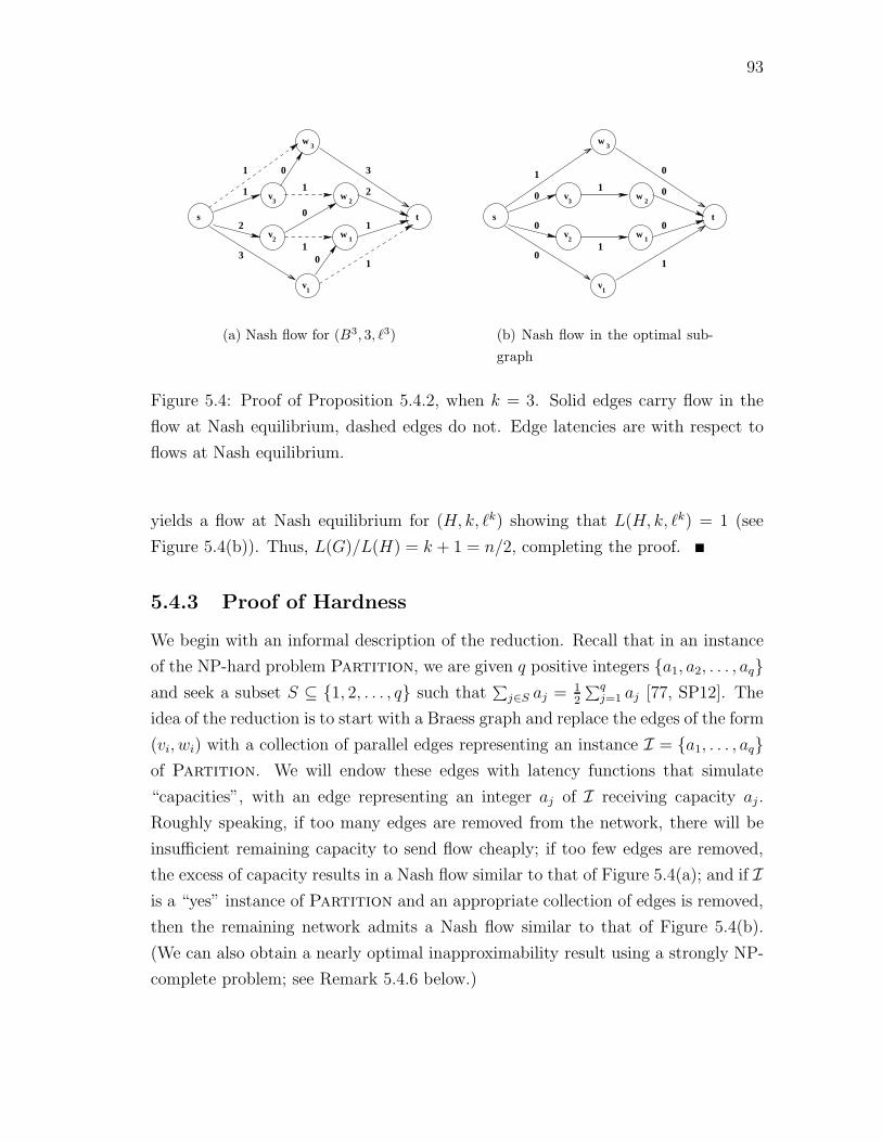
93

v1

v2

v3

w1

w2

w3

s t

1

1

3

2

1

2

3

1

0

10

0

1

(a) Nash flow for (B3, 3, 3)

v1

v2

v3

w1

w2

w3

s t

1

1

0

0

0

0

0

0

1

1

(b) Nash flow in the optimal sub-graph

Figure 5.4: Proof of Proposition 5.4.2, when k = 3. Solid edges carry flow in the

flow at Nash equilibrium, dashed edges do not. Edge latencies are with respect to

flows at Nash equilibrium.

yields a flow at Nash equilibrium for (H, k, k) showing that L(H, k, k) = 1 (see

Figure 5.4(b)). Thus, L(G)/L(H) = k + 1 = n/2, completing the proof.

5.4.3 Proof of Hardness

We begin with an informal description of the reduction. Recall that in an instance

of the NP-hard problem Partition, we are given q positive integers a1, a2, . . . , aqand seek a subset S ⊆ 1, 2, . . . , q such that

∑j∈S aj = 1

2

∑qj=1 aj [77, SP12]. The

idea of the reduction is to start with a Braess graph and replace the edges of the form

(vi, wi) with a collection of parallel edges representing an instance I = a1, . . . , aqof Partition. We will endow these edges with latency functions that simulate

“capacities”, with an edge representing an integer aj of I receiving capacity aj .

Roughly speaking, if too many edges are removed from the network, there will be

insufficient remaining capacity to send flow cheaply; if too few edges are removed,

the excess of capacity results in a Nash flow similar to that of Figure 5.4(a); and if Iis a “yes” instance of Partition and an appropriate collection of edges is removed,

then the remaining network admits a Nash flow similar to that of Figure 5.4(b).

(We can also obtain a nearly optimal inapproximability result using a strongly NP-

complete problem; see Remark 5.4.6 below.)

94

Theorem 5.4.3 For ε > 0, there is no (n/2 − ε)-approximation algorithm for

General Latency Network Design unless P = NP .

Proof. We prove that for any fixed n ≥ 2, there is no (n2 − ε)-approximation

algorithm for General Latency Network Design restricted to (multi)graphs

with n vertices. (We can also restrict our instances to be simple networks and

derive a nearly optimal inapproximability result—see Remark 5.4.5 below.) As in

the proof of Proposition 5.4.2, we may assume that n is even and at least four. Write

n = 2k + 2 for k ∈ N . We will show that an (n2− ε)-approximation algorithm for

graphs with n vertices enables us to differentiate between “yes” and “no” instances

of Partition in polynomial time.

Consider an instance I = ajqj=1 of Partition, with each aj a positive integer.

We may assume that each aj is even, scaling if necessary. Put A =∑q

j=1 aj ; the

traffic rate of interest to us is r = kA2

+k+1. Obtain a graph G from the kth Braess

graph Bk by replacing each edge of the form (vi, wi) by q parallel edges, and denote

these by e1i , e

2i , . . . , e

qi .

We now specify the edge latency functions , which are more complicated than

in the previous subsection. We require a sufficiently small constant δ (1/A(q + k)

is small enough) and a sufficiently large constant M (n/2 is large enough). In what

follows, the constant M should be interpreted as a substitute for +∞, and is used

to penalize a flow for violating an edge capacity constraint. We require the constant

δ to transform step functions (the type of function that would be most convenient

for our argument) into continuous functions (which are allowable in our model); δ

provides a small “window” in which to “smooth out” the discontinuities of a step

function. For each edge e of the form (vi, wi−1), (s, wk), or (v1, t), define e(x) = 1 for

x ≤ 1 and e(x) = M for x ≥ 1+δ (e may be defined arbitrarily on (1, 1+δ), subject

to the usual continuity and monotonicity restrictions). We say that these edges have

capacity 1. For an edge e of the form (wi, t) or (s, vk−i+1) (where i ∈ 1, . . . , k),define e(x) = 0 for x ≤ 1

2A + 1, e(x) = i when x = 1

2A + k+1

k, and e(x) = M for

x ≥ 12A + k+1

k+ δ; these edges have capacity 1

2A + k+1

k. Finally, for an edge e of the

form eji , define e(x) = 0 for x ≤ aj − δ, e(aj) = 1, and e(x) = M for x ≥ aj + δ;

thus eji has capacity aj . Each latency function can be described by a piecewise linear

function with a small (constant) number of rational breakpoints and slopes, and the

instance (G, r, ) can be constructed from I in polynomial time.

Analogous to the proof of Theorem 5.3.2, it suffices to prove the following two

statements: (i) if I is a “yes” instance, then G admits a subgraph H with L(H, r, ) =

95

1; and (ii) if I is a “no” instance, then L(H, r, ) ≥ n/2 for every subgraph H of G.

To prove (i), suppose that I admits a partition, and reindex the aj’s so that∑mj=1 aj = A/2 for some m ∈ 1, 2, . . . , q − 1. Obtain H from G by deleting all

edges of the form eji for j > m; thus, for each i = 1, . . . , k, the remaining edges of

the form eji have total capacity A/2. Define the paths Q1, . . . , Qk+1 as in the proof

of Proposition 5.4.2: for i = 2, . . . , k, Qi denotes the path s → vi → wi−1 → t,

Q1 is the path s → v1 → t, and Qk+1 is the path s → wk → t. Define a feasible

flow f as follows: for each i = 1, . . . , k and j = 1, . . . , m, route aj units of flow

on the unique path containing edge eji , and route 1 unit of flow on the path Qi for

i = 1, 2, . . . , k + 1. The flow f is at Nash equilibrium for (H, r, ) and proves that

L(H, r, ) = 1 (see Figure 5.5(a)).

In proving (ii), we first consider only subgraphs H that contains all edges not of

the form eji (i.e., H may be obtained from G by deleting only some of the parallel

edges); as we will see, this case captures all of the difficulties of the proof. There

are two subcases to consider.

Case 1: Suppose for each i = 1, . . . , k, the total capacity Ai of edges of the form eji

in H is at least A/2. Since I is a “no” instance and each aj is even, Ai ≥ A/2+2 for

each i. Then, define a flow f in G as follows: for each i = 1, . . . , k and j = 1, . . . , q

such that eji is present in H , route aj

Ai(A

2+ k+1

k) units of flow along the unique s-t

path containing eji . The flow f is at Nash equilibrium and proves that L(H) = n/2

(see Figure 5.5(b)).

Case 2: Suppose for some i ∈ 1, . . . , k, the total capacity Ai of edges of the

form eji in H is less than A/2 (and thus is at most A/2 − 2). Here, we will exploit

the fact that all edges of the network are (essentially) capacitated to prove that a

flow at Nash equilibrium must have large cost. Call an edge e oversaturated by a

flow f if fe exceeds the capacity of e by at least δ (and thus e(fe) = M ≥ n/2).

A key observation is that if f is at Nash equilibrium for (H, r, ) and oversaturates

some edge, then L(H, r, ) ≥ n/2. Now, since the total capacity of edges out of vi

is at most A/2 − 1 (recall (vi, wi−1) has capacity 1), any flow that places at leastA2−1+qδ units of flow on (s, vi) will oversaturate some edge out of vi. On the other

hand, the total capacity of edges incident to s is kA2

+ k + 2 = r + 1, so any feasible

flow must either place at least A2−1+qδ units of flow on (s, vi) or oversaturate some

other edge out of s (for δ sufficiently small). We conclude that any flow feasible for

(H, r, ) oversaturates at least one edge, and hence L(H) ≥ n/2.

96

v1

v2

v3

w1

w2

w3

s t

1

1 1

0

0

0

0

1

1 1

10

0

1

1

1

(a) A good Nash flow correspond-ing to a “yes” instance of Parti-

tion, with m = 2

v1

v2

v3

w1

w2

w3

s t

1

1

1

11

2

3

3

2

10

0

0

0 0

0 0

00

(b) A bad Nash flow in a networkwith excess capacity

Figure 5.5: Proof of Theorem 5.4.3. Solid edges carry flow in the flow at Nash

equilibrium, dashed edges do not. Edge latencies are with respect to flows at Nash

equilibrium.

Finally, suppose H fails to contain an edge that is not of the form eji . If for

some i ∈ 1, 2, . . . , k, the total capacity of edges of the form eji is at most A/2,

then the argument of Case 2 still applies to show that L(H) ≥ n/2—the previous

argument merely required that any feasible flow oversaturates some edge, and this

fact remains valid if we remove further edges. Also, if H fails to contain an edge

of the form (s, vi) or (wi, t), then simple capacity considerations show that any

feasible flow in H oversaturates some edge incident to s or t, respectively. If H

contains all edges of the form (s, vi) and (wi, t) and the total capacity of edges of

the form eji in H is at least A/2 for each i, then the argument of Case 1 applies (by

hypothesis, all edges used by the Nash flow in that case are present in H), showing

that L(H) = n/2. This exhausts all possible cases, and the proof is complete.

The matching upper and lower bounds of Theorems 5.4.1 and 5.4.3 have strong

negative consequences for the problem of detecting harmful extraneous edges, as in

the linear latency function setting (see Corollary 5.3.3). Defining an instance (G, r, )

with general latency functions and n vertices to be paradox-free if L(H, r, ) ≥L(G, r, ) for all subgraphs H of G and paradox-ridden if for some subgraph H in

G, L(H, r, ) = (n/2)−1L(G, r, ), we obtain the following corollary.

Corollary 5.4.4 Given an instance (G, r, ) with general latency functions that is

97

either paradox-free or paradox-ridden, it is NP-hard to decide whether or not (G, r, )

is paradox-ridden.

Remark 5.4.5 The reduction of Theorem 5.4.3 also shows that, for any constant

ε > 0, there is no O(n1−ε)-approximation algorithm for General Latency Net-

work Design restricted to simple graphs (unless P = NP ). To see why, choose a

positive integer k satisfying k > 1ε, and for a Partition instance I with q items,

mimic the previous reduction beginning with the Braess graph Bqkon 2qk + 2 ver-

tices. Subdividing all parallel edges in the resulting multigraph yields a simple graph

G (whose size is polynomial in that of I) with n = qk+1+2qk +2 vertices. Defining r

and as in the proof of Theorem 5.4.3, G has a subgraph H satisfying L(H, r, ) = 1

if I is a “yes” instance while L(H, r, ) ≥ qk +1 for every subgraph H if I is a “no”

instance. Thus, no O(n(k−1)/k)-approximation algorithm exists for General La-

tency Network Design restricted to simple graphs, unless P = NP .

Remark 5.4.6 The reduction of Theorem 5.4.3 makes use of the weakly NP-hard

problem Partition [77], and it thus reasonable to ask for approximation algorithms

with good performance guarantee but pseudopolynomial running time (running time

polynomial in the network size and in the unary representation of the numbers used

to describe the latency functions). Unfortunately, such an algorithm cannot exist

(unless P = NP ): the non-existence of an O(n1−ε)-approximation algorithm for

network design on simple graphs can also be derived from the more complicated

construction in the proof of Theorem 5.5.6 below, and this construction relies only

on the strongly NP-hard problem 2DDP of Section 5.3.

5.5 Polynomials of Bounded Degree:

An Approximability Threshold of Θ( plog p)

In this section, we aim to show that the strong hardness results of Sections 5.3

and 5.4 extend beyond the particular classes of linear and general latency functions,

and seem intrinsic to the problem of designing networks for selfish users. We will

focus on networks with latency functions that are polynomials of bounded degree,

but our techniques will also have consequences for networks possessing other types

of well-behaved latency functions.

As in Section 5.3, we begin by observing that our previous work bounding the

worst-case inefficiency of flows at Nash equilibrium yields an upper bound on the

98

performance guarantee of the trivial algorithm. Recall from Proposition 3.5.5 that

in an instance with polynomial latency functions of degree p (with all polynomial

coefficients nonnegative), the total latency of a flow at Nash equilibrium is at most

[1 − p · (p + 1)−(p+1)/p]−1 times that of any other feasible flow. For clarity, we will

work with the following weaker form of Proposition 3.5.5.

Corollary 5.5.1 There is a constant c1 > 0 so that the following statement holds:

if p ≥ 2 and (G, r, ) is an instance with polynomial latency functions of degree p for

which f ∗ is feasible and f is a flow at Nash equilibrium, then C(f) ≤ c1p

ln p· C(f ∗).

As with linear latency functions (see Corollary 5.3.1), we immediately obtain an

upper bound on the performance guarantee of the trivial algorithm for our network

design problem restricted to networks with polynomial latency functions of degree

p. We call this problem Polynomial(p) Latency Network Design.

Corollary 5.5.2 There is a constant c1 > 0 so that, for any p ≥ 2, the trivial algo-

rithm is a c1p

ln p-approximation algorithm for Polynomial(p) Latency Network

Design.

We next work toward a proof of a matching hardness result. As in Section 5.4,

we first give a family of networks (one network for each value of p ≥ 2) on which

the trivial algorithm performs poorly, and then describe how to obtain a general

inapproximability result.

Proposition 5.5.3 There is a constant c2 > 0 so that, for any p ≥ 2, the worst-case

performance guarantee of the trivial algorithm is at least c2p

ln pfor Polynomial(p)

Latency Network Design.

Proof. We will again make use of the Braess graphs of Subsection 5.4.2. In Sec-

tion 5.4, we exploited the fact that general latency functions can be arbitrarily steep

to construct a bad example for the trivial algorithm; here, we adapt the previous

argument as best we can, given that only low-degree polynomials are available to

us.

For a fixed integer p, define a set of latency functions k for the edges of Bk

as follows (where k is a parameter, depending on p, to be chosen later): for each

edge of the form e = (vi, wi), put ke(x) = 0; for an edge e of the form (vi, wi−1),

(s, wk), or (v1, t), put ke(x) = 1; for an edge e of the form (wi, t) or (s, vk−i+1)

put ke(x) = ixp. Next, consider the instance (Bk, k, k) and define paths P1, . . . , Pk

99

and Q1, . . . , Qk+1 as in Proposition 5.4.2. On one hand, routing one unit of flow

on each of P1, . . . , Pk yields a flow at Nash equilibrium for (Bk, k, k) showing that

L(Bk, k, k) = k + 1 (as in Figure 5.4(a)). On the other hand, if H is the subgraph

obtained from Bk by deleting all edges of the form (vi, wi), routing kk+1

units of flow

on each of Q1, . . . , Qk+1 yields a flow at Nash equilibrium for (H, k, k) showing that

L(H, k, k) = 1 + k( kk+1

)p (cf., Figure 5.4(b)). Thus,

L(H, k, k) = 1 + k(k

k + 1)p ≤ 1 + ke−p/(k+1).

For p sufficiently large, we may put k = p2 ln p

− 1 ≥ 1 to obtain L(H, k, k) ≤ 2

and L(Bk, k, k) = p2 ln p

; this completes the proof.

Remark 5.5.4 In the proof of Proposition 5.5.3, we have avoided optimizing con-

stants for the sake of readability. We will make this tradeoff repeatedly in the rest

of this section.

Finally, we extend our lower bound on the performance guarantee of the trivial

algorithm to an inapproximability result. This task is more difficult than in Sec-

tion 5.4; a crucial part of the hardness proof of that section leveraged the fact that

general latency functions can model edge capacities. This is not entirely possible

with low-degree polynomials, and we are forced instead to adapt the arguments

of Section 5.3 to larger Braess graphs; in particular, our reduction is from the 2

Directed Disjoint Paths problem rather than from Partition. In essence, re-

stricting the allowable class of latency functions forces us to encode the intractability

of an NP-hard problem into the network topology of a network design instance rather

than into the edge latency functions.

In preparation for the reduction, we require one preliminary result. The next

proposition is a special case of a theorem of Hall [83].

Proposition 5.5.5 ([83]) Let G be a network with polynomial latency functions

and a single source-destination pair. Then L(G, r, ) is a nondecreasing function of

r.

We can now prove that designing networks for selfish users is hard in networks

with polynomial edge latency.

Theorem 5.5.6 There is a constant c3 > 0 so that the following statement holds: if

p ≥ 2 and ε > 0, then no (c3p

ln p− ε)-approximation algorithm for Polynomial(p)

Latency Network Design exists, unless P = NP .

100

Proof. Fix a sufficiently large integer p, and put k = p16 ln p

− 1 (which is at least

1 for large enough p). For any ε > 0, we will show that a (k5− ε)-approximation

algorithm for Polynomial(p) Latency Network Design enables us to differ-

entiate between “yes” and “no” instances of the 2 Directed Disjoint Paths

(2DDP) problem in polynomial time (for a definition of 2DDP, see the proof of

Theorem 5.3.2).

Consider an instance I = G, s1, s2, t1, t2 of 2DDP; we construct an instance

of Polynomial(p) Latency Network Design (G′, k, ) as follows (illustrated

in Figure 5.6). To define the graph G′, we begin with k copies of G; call them

G1, . . . , Gk and denote the copy of si (ti) in Gj by sji (tji ). Next, add auxiliary

vertices s, t, v1, . . . , vk−1, and w1, . . . , wk−1. The edge set of G′ is as follows:

• each Gi inherits the edge set of G

• for i = 1, . . . , k− 1, we include edges from s to vi, from vi to si2 and si+1

1 , from

ti2 and ti+11 to wi, and from wi to t

• we include edges (s, s11), (s, sk

2), (t11, t), (tk2, t).

We define latency functions on the edges of G′ as follows:

(A) for edges of the form (vi, si2) or (ti+1

1 , wi), put (x) = 1

(B) for edges (s, s11) and (tk2, t), put (x) = 2 + (1 + 1

k)pxp

(C) for (s, sk2) and (t11, t), put (x) = 1 + k(4(k+1)

4k+1)pxp

(D) for i = 1, . . . , k − 1 and edges (s, vi) and (wk−i, t), put (x) = i(4(k+1)4k+1

)pxp

(E) for edges of the form (vi, si+11 ) or (ti2, wi), put (x) = 2 + (2 + 2

k)pxp

(F) for edges in G1, . . . , Gk, put (x) = 0.

We will call edges of the form (vi, si2) or (ti+1

1 , wi) type A edges, and so forth. It is

clear that (G′, k, ) can be constructed from I in polynomial time.

Next, we claim that if I is a “yes” instance of 2DDP, then there is a subgraph

H of G′ satisfying L(H, k, ) ≤ 5. To see why, let P ∗1 and P ∗

2 denote vertex-disjoint

s1-t1 and s2-t2 paths in G. Deleting all edges in G′ that lie in some copy Gi of G

but not on (the corresponding copy of) either P ∗1 or P ∗

2 , we obtain a subgraph H of

G′ that is the union of 2k distinct s-t paths. Routing kk+1

units of flow on the path

containing s11 and t11 and on the path containing sk

2 and tk2, and k2(k+1)

units of flow

101

t2

t

C

D

D

B C

D

D

BG

G1t

s1

s2

s

Gs1

s2

2t

1t

w

2

1t

2t

s1

v

s2

A

A

A

A

E

E

E

E

1

2

3

1

w2

1v

Figure 5.6: Proof of Theorem 5.5.6. Construction of (G′, k, ) when k = 3. Edges

are labeled with their edge type.

on each of the other 2k−2 paths, we obtain a flow at Nash equilibrium for (H, k, ).

This flow proves that

L(H, k, ) = 4 + k

(4(k + 1)

4k + 1

k

k + 1

)p

= 4 + k(1 − 1

4k + 1

)p

≤ 4 + ke−p/(4k+1) ≤ 5,

with the picture of this Nash flow somewhat analogous to Figure 5.4(b).

Finally, we show that if I is a “no” instance of 2DDP, then L(H, k, ) ≥ k for all

subgraphs H of G′. We will prove this in two steps. First, we will show that unless

H contains most of the edges in G′, “capacity considerations” (similar to those used

in the proof of Theorem 5.4.3) imply that L(H) is large. Second, we show that if H

contains most of the edges in G′, then the flow at Nash equilibrium in H is similar

to the bad Nash flow of Proposition 5.5.3, again showing L(H) to be large.

Fix a subgraph H of G′ containing an s-t path, and let f be an acyclic Nash

flow in (H, k, ) (see Proposition 2.6.2). We claim that if some type A or C edge

of G′ does not carry flow in f (in particular, if some such edge is not in H), then

L(H) ≥ k. We will prove the claim for an edge of the form (vi, si2); the argument

for an edge of the form (ti+11 , wi) is symmetric, and the argument for type C edges

is similar (and easier).

102

To prove this claim, we first observe that many edges of H are essentially ca-

pacitated, in the following sense. We assert that any of the following events forces

L(H) ≥ p ≥ k (using that L(H) ≥ e(fe) for any edge e with fe > 0):

(1) fe ≥ 8k+18(k+1)

for a type B edge e

(2) fe ≥ 2k+12(k+1)

for an edge e of type C or D

(3) fe ≥ 4k+18(k+1)

for a type E edge e.

For example, we can derive(4(k + 1)

4k + 1

2k + 1

2(k + 1)

)p

=(1 +

1

4k + 1

)p

>[e1/(8k+2)

]p= ep/(8k+2) ≥ p,

proving (2). The calculations for (1) and (3) are similar, so we omit them.

Now assume that edge (vi, si2) does not carry any flow in f . Then, either event

(3) occurs (with edge (vi, si+11 )) or else edge (s, vi) carries at most 4k+1

8(k+1)units of

flow; assume the latter. We claim that in this case, event (1) or event (2) must

occur with some edge incident to s. For if not, edges incident to s carry at most

(k − 1)2k + 1

2(k + 1)+

4k + 1

8(k + 1)+

8k + 1

8(k + 1)=

8k2 + 8k − 2

8(k + 1)< k

units of flow, contradicting that f is an s-t flow carrying k units of flow. We conclude

that if edge (vi, si2) does not carry flow in f , then some event of the form (1), (2),

or (3) occurs, proving that L(H) ≥ k.

It remains to consider subgraphs H of G′ in which all edges of type A or C carry

flow in the Nash flow f of (H, k, ), and to make use of our hypothesis that I is a

“no” instance of 2DDP. The presence of these edges in H (all of which lie on s-t

paths in H , since they carry flow in the acyclic flow f), together with the assumption

that I is a “no” instance, imply that for each i = 1, 2, . . . , k there is an s-t path

Pi in H containing the vertices si2 and ti1 (cf., the proof of Theorem 5.3.2). Letting

r = k(4k+1)4(k+1)

< k, the following flow is then at Nash equilibrium for (H, r, ): for

i = 1, 2, . . . , k route 4k+14(k+1)

units of flow on Pi. This flow shows that L(H, r, ) = k+3

(this Nash flow is essentially the same as the bad Nash flow of Proposition 5.5.3).

By Proposition 5.5.5, L(H, ·, ) is an increasing function of the traffic rate (with H,

fixed); hence, L(H, k, ) ≥ k + 3.

We have shown that if I is a “no” instance of 2DDP, then L(H, k, ) ≥ k for all

subgraphs H of G′, and the proof is complete.

103

Remark 5.5.7 The results of this section can be extended to networks with other

types of latency functions with only minor modifications to the proofs. For example,

in Sections A.1 and A.2 we introduce the notion of the incline of an instance (intu-

itively, a real number γ ≥ 1 that measures the “steepness” of the network latency

functions) and prove that the price of anarchy in instances with incline γ is at most

γ. By the same argument as in Corollaries 5.3.1 and 5.5.2, this implies that the

trivial algorithm is a γ-approximation algorithm for instances with incline at most

γ. A straightforward modification of the proof of Theorem 5.5.6 shows that there

is a constant c > 0 such that, for each γ ≥ 1 and ε > 0, there is no (c · γ − ε)-

approximation algorithm for instances with incline at most γ (unless P = NP ). We

leave the details of the proof and further extensions of this sort to the interested

reader.

Chapter 6

Stackelberg Routing

6.1 Introduction

In this chapter, we pursue a second approach to coping with selfishness. In many

networks, there will be a mix of “selfishly controlled” and “centrally controlled”

traffic—that is, the network is used by both selfish individuals and some central

authority. For example, clients of a network may be charged at two different prices:

clients paying the higher price are given access to the network and the ability to route

their own traffic (presumably along a minimum-latency path), while clients paying

only the “bargain rate” can use the network but have no control over how their

traffic is routed (and thus this traffic qualifies as centrally controlled). Also, Korilis

et al. [105] consider networks that allow a large customer to set up a so-called virtual

private network of guaranteed and preassigned virtual paths for ongoing use [21],

and argue that the bandwidth needed for a virtual private network may be viewed as

centrally controlled (with the paths chosen by the network manager) while individual

users of the network continue to behave in a selfish and independent fashion.

We investigate the following question: given a network with centrally and self-

ishly controlled traffic, how should centrally controlled traffic be routed to induce

“good” (albeit selfish) behavior from the noncooperative users? This indirect ap-

proach to controlling selfish behavior has several appealing aspects: no communi-

cation is required between network users and an algorithm, no notion of currency

is needed (cf., the approach of algorithmic mechanism design [136, 137, 155]), no

resources need to be added to or removed from the network, and the routing of

centrally controlled traffic is often easily modified as the amount of traffic evolves

over time.

104

105

6.1.1 Summary of Results

We consider a game in which the roles of different players are asymmetric. One

player (responsible for routing the centrally controlled traffic and interested in min-

imizing total latency) acts as a leader, in that it may hold its routing (its strategy)

fixed while all other players (the followers) react independently and selfishly to the

leader’s strategy, reaching a Nash equilibrium relative to it. These types of games,

called Stackelberg games, and the resulting Stackelberg equilibria have been well

studied in the game theory literature (see Subsection 6.1.3 below).

We study the following questions:

(1) among all leader strategies for a given network, can we characterize and/or

compute the strategy inducing the Stackelberg equilibrium—that is, the equi-

librium of minimum total latency?

(2) what is the worst-case ratio between the total latency of the Stackelberg equi-

librium and that of the optimal routing of all of the traffic?

For networks with arbitrary edge latency functions but consisting only of two

nodes and a collection of parallel links, we give a simple algorithm for computing

a leader strategy that induces an equilibrium with total latency no more than 1β

times that of the minimum-latency flow, where β denotes the fraction of traffic that

is centrally controlled. This algorithm runs in polynomial time provided the net-

work latency functions are standard (see Definition 2.3.5). We also show that no

stronger guarantee is possible in networks of parallel links, and that this guaran-

tee cannot be achieved in general networks. Thus, in a network of parallel links, a

manager controlling a constant fraction of the network traffic can induce an equi-

librium with total latency at most a constant-factor larger than that incurred by

the minimum-latency flow. This result stands in sharp contrast to our results about

Nash equilibria, as the nonlinear variant of Pigou’s example (Subsection 2.4.4) shows

that the total latency of a flow at Nash equilibrium can be arbitrarily larger than

that of a minimum-latency flow, even in networks of parallel links.

For networks of parallel links in which every edge latency function is linear in the

edge congestion, we give a simple algorithm that runs in O(m2) time and computes

a strategy inducing an equilibrium with total latency no more than 43+β

times that

of the minimum-latency flow, where β is the fraction of centrally controlled traffic

and m is the number of edges. We again show that no stronger guarantee is possible.

106

Finally, we consider the optimization problem of computing the strategy inducing

the Stackelberg equilibrium and show that it is NP-hard, even in the special case of

networks of parallel links with linear latency functions.

6.1.2 Comparison to the Price of Anarchy

The results of this chapter give a (sharp) trade-off between a minimum-latency flow

and a flow at Nash equilibrium (as a function of the fraction of the traffic that is

centrally controlled) in networks of parallel links, in the following sense. In Chapter 3

we showed that a flow at Nash equilibrium can be arbitrarily more costly than the

minimum-latency flow, but if every edge latency function is linear then the total

latency of a Nash flow is no more than 43

times that of a minimum-latency flow.

Thus, the results of this chapter reduce to those of Chapter 3 when β = 0, give the

trivial result that the Stackelberg equilibrium for β = 1 is the minimum-latency flow,

and quantify the worst possible ratio between the cost of the Stackelberg equilibrium

(in some sense, a “mixture” of a Nash flow and a minimum-latency flow) and the

cost of a minimum-latency flow for all intermediate values of β.

Our approach also adds an algorithmic dimension to our work in Part II bounding

the price of anarchy, in that one aspect of our analysis of Stackelberg equilibria is the

design of algorithms for efficiently computing good Stackelberg strategies. Further,

while optimal and Nash flows can be characterized and computed efficiently via

convex programming (see Propositions 2.3.1 and 2.5.1)—a fact that was crucial for

our work bounding the price of anarchy—the hardness result of this chapter implies

that no such characterization of Stackelberg equilibria is possible. With the central

approach of Part II ruled out, we will require new techniques for bounding the

inefficiency of Stackelberg equilibria.

6.1.3 Related Work

Stackelberg games and Stackelberg equilibria have been thoroughly studied in the

game theory literature (see, for example, [75] or [13, §3.6] for an introduction

and [184] for their origin) and have previously been applied to problems in competi-

tive facility location [153], networking [53, 54, 58, 104], and more general continuous-

time systems (see the surveys of Cruz [41, 42], the book of Bagchi [12], and the

references therein). With the exception of [53, 104], however, the leader/follower

hierarchy has been used to model classes of selfish users with different priority lev-

107

els; this setting differs from ours in that no user is interested in optimizing system

performance.1 The note of Douligeris and Mazumdar [53] is concerned only with

experimental results on the effectiveness of Stackelberg strategies. The paper of

Korilis et al. [104], while more similar in spirit to ours, focuses on deriving necessary

and sufficient conditions (on the number of selfish users, the fraction of the traffic

that is centrally controlled, etc.) for the existence of a leader strategy inducing an

optimal routing of all of the traffic; moreover, only one type of latency function is

considered. By contrast, we are interested in simple leader strategies that always in-

duce optimal or near-optimal behavior from the network users for any set of latency

functions.

6.1.4 Organization

In Section 6.2 we extend our basic traffic model to accommodate Stackelberg equilib-

ria. In Section 6.3 we introduce three simple algorithms for computing Stackelberg

strategies in networks of parallel links. In Sections 6.4 and 6.5, we prove that

our third algorithm achieves the best-possible worst-case performance guarantee for

networks of parallel links with general and linear latency functions, respectively.

In Section 6.6, we prove that computing the optimal strategy is NP-hard, even in

networks of parallel links with linear latency functions.

6.2 Stackelberg Strategies and Induced Equilibria

In this section we define our notion of a Stackelberg game and consider two ex-

amples. We will focus on networks in which all traffic shares a common source

and destination, although the definitions of this section are easily extended to a

multicommodity setting.

Recall we desire a hierarchical game, where a leader routes centrally controlled

traffic and, holding this strategy fixed, the network users react in a noncooperative

and selfish manner. This idea is formalized in the next two definitions. By a

Stackelberg instance (G, r, , β), we mean a single-commodity instance (G, r, ) in

the sense of Section 2.1 together with a parameter β ∈ [0, 1] specifying the fraction

of the network traffic that is centrally controlled.

1Traditionally, Stackelberg games model selfish users with asymmetric roles; our use of them issomewhat unconventional.

108

Definition 6.2.1 A (Stackelberg) strategy for the Stackelberg instance (G, r, , β) is

a flow feasible for (G, βr, ).

Definition 6.2.2 Let f be a strategy for Stackelberg instance (G, r, , β), and define

e by e(x) = e(fe + x) for each edge e ∈ E. An equilibrium induced by strategy f

is a flow g at Nash equilibrium for the instance (G, (1 − β)r, ). We then say that

f + g is a flow induced by f for (G, r, , β).

Existence and essential uniqueness of induced equilibria follow easily from Propo-

sitions 2.2.4 and 2.5.1.

Proposition 6.2.3 Let f be a strategy for a Stackelberg instance with continuous,

nondecreasing latency functions. Then there exists a flow induced by f , and any two

such induced flows have equal cost.

The following simple observation will be useful in Sections 6.4 and 6.5.

Lemma 6.2.4 Let f be a strategy for Stackelberg instance (G, r, , β) inducing equi-

librium g, where G is a network of parallel links. Let G′ denote the subgraph induced

by the edges e on which ge > 0. Then f + g, restricted to the edges of G′, is a

flow at Nash equilibrium for the instance (G′, r′, ), where r′ =∑

e∈G′(fe + ge). In

particular, all edges e on which ge > 0 have a common latency with respect to f + g.

We next consider two examples that demonstrate both the usefulness and the lim-

itations of Stackelberg strategies. First consider Pigou’s example (Subsection 1.2.1).

Recall that in the absence of centrally controlled traffic, a Nash flow incurs total

latency 43

times that of the optimal flow. Suppose instead that half of the traffic

is controlled by the network manager (i.e., that β = 12) and consider the strategy

f of routing all centrally controlled traffic on the top edge (the edge with latency

function (x) = 1). Then, as all remaining traffic will be routed on the lower edge

in the equilibrium induced by f , the flow induced by f is precisely the minimum-

latency flow. Thus, in this particular instance, total latency can be minimized via

a Stackelberg strategy.

Now consider a small modification to Pigou’s example, in which we replace the

latency function of the lower edge with the latency function (x) = 2x. The flow

at Nash equilibrium puts half of the traffic on each edge for a cost of 1, while the

optimal flow routes only 14

of the traffic on the lower edge, for a cost of 78. On the

other hand, if we again allow the network manager to route half of the traffic, we

109

see that for any strategy f , the flow induced by f is the flow at Nash equilibrium

and hence is not optimal. In this example, there is no available strategy by which

the network manager can improve network performance.

6.3 Three Stackelberg Strategies

6.3.1 Two Natural Strategies

We begin our investigation of Stackelberg strategies for networks of parallel links by

considering two natural approaches that provide suboptimal performance guaran-

tees. To motivate our results in the simplest possible way, throughout this subsection

we will consider examples with linear latency functions in which half of the traffic

is centrally controlled (β = 12).

First consider the following strategy for an instance (G, r, , 12): if f ∗ is the

minimum-latency flow for instance (G, 12r, ), put f = f ∗. In words, we choose

the strategy of minimum cost (ignoring the existence of traffic that is not centrally

controlled). We call this the Aloof strategy since it refuses to acknowledge the rest

of the traffic in the network. Pigou’s example (Subsection 1.2.1) shows that this

strategy performs quite poorly: in that network, the Aloof strategy routes all flow

on the bottom edge (the edge with latency function (x) = x) and in the induced

flow all traffic is routed on the bottom edge. Thus, the Aloof strategy induces the

(inefficient) Nash flow while the strategy that routes all centrally controlled traffic

on the top edge induces the optimal flow. Applying this type of argument to the

nonlinear variant of Pigou’s example (Subsection 2.4.4), it is also easy to see that

the Aloof strategy can perform arbitrarily badly in networks with general latency

functions.

A second attempt at a good strategy might be as follows: if f ∗ is the minimum-

latency flow for (G, r, ), put f = 12f ∗. We call this the Scale strategy, since it is

simply the optimal flow, suitably scaled. To understand why we should be dissatis-

fied with the Scale strategy, consider the two-node, two-link example with latency

functions 1(x) = 1 and 2(x) = 32x and traffic rate 1. The minimum-latency flow

routes 23

of the flow on the first link and the rest on the second link (with total cost56), so the Scale strategy will route 1

3units of flow on the first link and 1

6units on

the second link. All selfish traffic is then routed on the second link, inducing the

flow with 13

units of flow on the first link and the rest on the second, having cost

110

1. It would appear that the Scale strategy routed too much flow on the second link

(since selfish traffic flocked to it, anyways); indeed, the strategy that instead routes

all centrally controlled traffic on the first link induces a flow with the superior cost

of 78.2

6.3.2 The Largest Latency First (LLF) Strategy

Intuitively, both the Aloof and Scale strategies suffer from a common flaw: both

route traffic on edges that will subsequently be inundated in any induced equilibrium

while routing too little traffic on edges that selfish users are prone to ignore. This

observation suggests that a good strategy should give priority to the edges that

are least appealing to selfish users—edges with relatively high latency. With this

intuition in mind, the following strategy for a Stackelberg instance (G, r, , β) defined

on a network of m parallel links (which we call the Largest Latency First or LLF

strategy) should seem natural:

(1) Compute a minimum-latency flow f ∗ for (G, r, ).

(2) Label the edges of G from 1 to m so that 1(f∗1 ) ≤ · · · ≤ m(f ∗

m).

(3) Let k ≤ m be minimal with∑m

i=k+1 f ∗i ≤ βr.

(4) Put fi = f ∗i for i > k, fk = βr −∑m

i=k+1 f ∗i , and fi = 0 for i < k.

We will say that an edge i is saturated by a strategy f if fi = f ∗i . Thus, the LLF

strategy saturates edges one-by-one (in order from the largest latency with respect to

f ∗ to the smallest) until there is no centrally controlled traffic remaining. Note that

as long as all link latency functions are standard (see Definition 2.3.5), Fact 2.3.6

implies that the LLF strategy can be computed in polynomial time (the bottleneck

is step (1)); in Section 6.5 we will see that it can be computed in O(m2) time when

every latency function is linear.3

The next two sections are devoted to proving that the LLF strategy always

induces a flow with near-optimal total latency.

2In addition, a slightly more complicated example shows that the Scale strategy can performarbitrarily badly in networks with general latency functions.

3We ignore the fact that an optimal flow can only be computed up to an arbitrarily smalladditive factor (see Fact 2.3.6), as this does not affect our results in any significant way.

111

6.4 Arbitrary Latency Functions: A Performance

Guarantee of 1/β

In this section we prove that the LLF strategy induces a near-optimal flow for net-

works of parallel links with arbitrary latency functions. We note that no performance

guarantee is possible for such networks in the absence of centrally controlled traffic:

without additional restrictions on edge latency functions, the Nash flow may incur

arbitrarily more latency than the optimal flow (as shown by the nonlinear variant

of Pigou’s example). Thus, the benefit of a leader (and of a carefully chosen leader

strategy) is particularly striking in this general setting.

A simple variation on previous examples demonstrates the limits of Stackelberg

strategies. In a two-node, two-link instance with β = 12

and latency functions

1(x) = 1 and 2(x) = 2pxp for p ∈ Z+, any Stackelberg strategy induces the Nash

flow (half of the flow on each link, with cost 1) while the minimum-latency flow

routes 12+ δp units of flow on the first link and the rest on the second link, for a cost

of 12+ εp with δp, εp → 0 as p → ∞. Thus the best induced flow may be (arbitrarily

close to) twice as costly as the optimal flow. Similar examples show that for any

β ∈ (0, 1), the best induced flow may be 1β

times as costly as the optimal flow.

The main result of this section is that the LLF strategy always induces a flow

of cost no more than 1β

times that of the minimum-latency flow. A rough outline

of the proof is as follows. Our goal is to exploit the iterative structure of the LLF

strategy and proceed by induction on the number of edges. If the LLF strategy

first saturates the mth edge (with the ordering of edges as in the description of the

LLF strategy), a natural idea is to apply the inductive hypothesis to the remainder

of the LLF strategy on the first m − 1 edges to derive a performance guarantee.

This idea nearly succeeds, but there are two difficulties. First, it is possible that

the LLF strategy fails to saturate any edges; we will see below that this case is easy

to analyze and causes no trouble. Second, in order to obtain a clean application

of the inductive hypothesis to the first m − 1 edges, we require that the optimal

and LLF-induced flows route the same total amount of flow on these edges—i.e.,

that the LLF-induced equilibrium eschews the mth edge.4 We resolve this difficulty

with the following lemma, which states that if the LLF strategy saturates the mth

edge, then some induced equilibrium routes all traffic on the first m− 1 edges—this

4This can fail in trivial cases, such as in a two-node, two-link network in which both edges havelatency function (x) = 1.

112

suffices for our purposes, since different induced flows have equal cost.

Lemma 6.4.1 Let (G, r, , β) denote a Stackelberg instance on a network of m par-

allel links with optimal flow f ∗, and label the edges of G from 1 to m so that

m(f ∗m) ≥ i(f

∗i ) for all i ∈ 1, 2, . . . , m. If f is a strategy with fm = f ∗

m, then

there exists an induced equilibrium g with gm = 0.

Proof. Consider an arbitrary induced equilibrium g and suppose gm > 0. Roughly

speaking, the idea is to prove that this scenario only occurs when several latency

functions (that of the mth edge, and others) are locally constant; then, traffic routed

on edge m in the induced equilibrium can be evacuated to other edges with locally

constant latency functions to provide a new induced equilibrium.

Formally, let L = m(fm + gm) = m(f ∗m + gm) denote the common latency with

respect to f + g of every edge with gi > 0 (see Lemma 6.2.4). We must have

m(f ∗m) ≥ L; otherwise i(f

∗i ) < L for all i yet i(fi + gi) ≥ L for all i, contradicting

that f ∗ and f + g are flows at the same rate. Thus, since m is nondecreasing, m is

locally constant: m is equal to L on [f ∗m, f ∗

m + gm].

Next, let E ′ denote the subgraph of edges on which fi +gi < f ∗i ; since fm +gm >

f ∗m, E ′ is non-empty. For i ∈ E ′, we have i(fi + gi) ≥ L, i(f

∗i ) ≤ m(f ∗

m) = L,

and i nondecreasing; hence, i is equal to L on [fi + gi, f∗i ]. Since f ∗ and f + g are

flows at the same rate, we must have∑

i∈E′[f ∗i − (fi + gi)] ≥ gm. Finally, consider

modifying g as follows: move all traffic previously routed on edge m to edges in

E ′, subject to the constraint fi + gi ≤ f ∗i . We have already observed that there is

sufficient “room” on edges in E ′ for this operation, and that all latency functions are

constant in the domain of our modifications. We have thus exhibited a new induced

equilibrium with no traffic routed on edge m, completing the proof.

We are now prepared to prove the main result of this section.

Theorem 6.4.2 Let I = (G, r, , β) denote a Stackelberg instance on a network of

parallel links. If f is an LLF strategy for I inducing equilibrium g and f ∗ is a

minimum-latency flow for the instance (G, r, ), then C(f + g) ≤ 1βC(f ∗).

Proof. We proceed by induction on the number of edges m (for each fixed m, we

will prove the theorem for arbitrary , r, and β). The case of a single edge is trivial.

Fix a Stackelberg instance I = (G, r, , β) with at least two edges, and let f ∗

denote a minimum-latency flow for the instance (G, r, ) and f the corresponding

LLF strategy. Label the edges 1 to m so that 1(f∗1 ) ≤ 2(f

∗2 ) ≤ · · · ≤ m(f ∗

m).

113

By scaling, we may assume that r = 1 (use latency functions with i(x) = i(rx)

otherwise). Let L denote the common latency with respect to f + g of every edge

with gi > 0 (see Lemma 6.2.4).

Case 1: Suppose gk = 0 for some edge k. Let E1 denote the edges i for which

gi = 0 and E2 the edges for which gi > 0; both of these sets are non-empty. Let

G1 and G2 denote the corresponding subgraphs of G. For j = 1, 2 let βj denote the

amount of centrally controlled traffic routed on edges in Ej and Cj the cost incurred

by f + g on edges in Ej . By Lemma 6.2.4, C2 = (1 − β1)L and C1 ≥ β1L. Now, f ∗

restricted to E2 is an optimal flow for (G2, 1−β1) and hence f restricted to E2 is an

LLF strategy for the instance I2 = (G2, 1 − β1, β′) where β ′ = β2

1−β1. Applying the

inductive hypothesis to I2 and using the fact that f ∗i ≥ fi = fi + gi for all i ∈ E1,

we obtain

C(f ∗) ≥ C1 + β ′C2.

Proving that C(f + g) ≤ 1βC(f ∗) thus reduces to showing

β(C1 + C2) ≤ C1 + β ′C2.

Since β ≤ 1 and C1 ≥ β1L, it suffices to prove this inequality with C1 replaced by

β1L. Writing C2 = (1 − β1)L and β ′ = β2

1−β1and dividing through by L, we need

only check that

β(β1 + (1 − β1)) ≤ β1 +β2

1 − β1

(1 − β1)

which clearly holds (both sides are equal to β).

Case 2: Suppose gi > 0 for every edge i, so C(f + g) = L. We may assume that

the LLF strategy failed to saturate edge m (otherwise, by Proposition 6.2.3, we can

finish by applying the previous case to the better-behaved induced flow guaranteed

by Lemma 6.4.1). Thus, β < f ∗m.

As in the proof of Lemma 6.4.1, we must have m(f ∗m) ≥ L; otherwise, i(f

∗i ) < L

for all edges i while i(fi +gi) = L for all i, contradicting that f ∗ and f +g are flows

at the same rate. Having established that edge m has large latency with respect to

f ∗ and that f ∗m is fairly large, it is now a simple matter to lower bound C(f ∗):

C(f ∗) ≥ f ∗mm(f ∗

m) ≥ βL = βC(f + g).

114

Remark 6.4.3 Theorem 6.4.2 applies only to networks of parallel links, and the

proof makes crucial use of the “decomposable” nature of such networks. On the

other hand, the guarantee of Theorem 6.4.2 cannot be extended to general network

topologies (cf., our work in Sections 3.3–3.4); even in the four-node network of

Braess’s Paradox (Figure 2.2), a network manager controlling a β fraction of the

traffic cannot in general induce a flow with cost at most a 1β

factor times that of the

minimum-latency flow (see Section B.3).

6.5 Linear Latency Functions: A Performance

Guarantee of 4/(3 + β)

6.5.1 Properties of the Nash and Optimal Flows

In this subsection we undertake a deeper study of Nash and optimal flows for in-

stances on networks of parallel links with linear latency functions. The results of

this subsection will be instrumental in proving a stronger performance guarantee for

the LLF strategy for these instances.

Fix a network G of m parallel links with linear latency functions (so that e(x) =

aex + be for each e ∈ E with ae, be ≥ 0) and label them from 1 to m so that

b1 ≤ b2 ≤ · · · ≤ bm. We may assume that at most one edge has a constant latency

function (ai = 0) since all but the one with smallest b-value can be safely discarded;

under this assumption, the Nash and optimal flows are always unique. We may

similarly assume that an edge with a constant latency function is the mth edge.

Our first goal is to understand the structure of the Nash flow f as a function

of the rate r. It is useful to imagine r increasing from 0 to a large value, with the

corresponding Nash flow changing in a continuous fashion; an intuitive description

of this process is as follows. Initially, when r is nearly zero, all traffic is routed on the

edge having the smallest constant term. Once the first edge is sufficiently congested,

the second edge looks equally attractive (this occurs when a1f1 +b1 = b2—i.e., when

the amount of flow on the first edge is b2−b1a1

). Subsequent traffic will be routed on

both of the first two edges, at rates proportional to 1a1

and 1a2

(traffic will be routed

so that these two edges continue to have equal latency). Once (b3 − b2)(1a1

+ 1a2

)

further units of traffic have been routed on the first two edges, the third edge will be

equally attractive and new traffic will be spread out among the first three edges, and

so on. We may thus envision the Nash flow as being constructed in phases: within

115

phase i traffic is routed on the first i edges according to fixed relative proportions

and at the end of the phase (after enough new flow has been routed) an additional

edge is put into use.

We now formalize this intuitive description of the Nash flow f . For i = 1, . . . , m,

let vi denote the m-vector ( 1a1

, 1a2

, . . . , 1ai

, 0, 0, . . . , 0) ∈ Rm+ ; if am = 0 put vm =

(0, 0, . . . , 1). The vector vi should be interpreted as a specification of the way traffic is

routed on the first i edges during the ith phase. Next, define δi for i = 0, 1, . . . , m−1

inductively by δ0 = 0 and δi = min(bi+1 − bi)‖vi‖1, r − ∑i−1j=0 δi ≥ 0 (where ‖·‖1

denotes the L1-norm of a vector). We also put δm = r − ∑m−1j=0 δi. The scalar δi

should be interpreted as the total amount of traffic routed in the ith phase. We can

then describe f as follows (where we interpret the m-vector f as a function on the

edges of G in the obvious way).

Lemma 6.5.1 Let I be an instance on a network of m parallel links with linear

latency functions, as above. Then the Nash flow for I is given by

f =m∑

i=1

δivi

‖vi‖1

.

Our characterization of optimal flows (Proposition 2.3.1 and Corollary 2.3.2)

yields an analogous result for computing them by an explicit formula. Note that

when a latency function has the form (x) = ax+b, the corresponding marginal cost

function (see Section 2.3) is ∗(x) = 2ax + b. Recalling from Corollary 2.3.2 that an

optimal flow is simply a flow at Nash equilibrium with respect to latency functions

∗, we see that the optimal flow is created by the same process as the Nash flow,

except that new edges are incorporated at a more rapid pace so as to spread traffic

over a wider range of edges (and thus achieve a smaller total latency).

Formally, let vi be as above and define δ∗i inductively by δ∗0 = 0, δ∗i = min12(bi+1−

bi)‖vi‖1, r−∑i−1

j=0 δ∗i , and δ∗m = r−∑m−1j=0 δ∗i . Letting f ∗ denote the minimum-latency

flow for (G, r, ), the analogue of Lemma 6.5.1 is as follows.

Lemma 6.5.2 Let I be an instance on a network of m parallel links with linear

latency functions, as above. Then the optimal flow for I is given by

f ∗ =m∑

i=1

δ∗ivi

‖vi‖1

.

Lemmas 6.5.1 and 6.5.2 have several useful corollaries. We summarize them

below.

116

Corollary 6.5.3 Let G be a network of m parallel links with linear latency func-

tions, with at most one edge having constant latency. Label the edges of G from 1

to m so that if i(x) = aix + bi, then bi is nondecreasing in i. Then:

(a) If f ∗ and f denote optimal and Nash flows for (G, r, ), then f ∗m ≥ fm.

(b) If f ∗ and f denote optimal and Nash flows for (G, r, ), then f ∗1 ≤ f1 ≤ 2f ∗

1 .

(c) If f ∗ is the optimal flow for (G, r, ) and f ∗ is the optimal flow for (G, r, )

with r ≥ r, then f ∗i ≥ f ∗

i for each edge i.

(d) For any rate r, the optimal and Nash flows for (G, r, ) can be computed in

O(m2) time.

Proof. Parts (c) and (d) are immediate from Lemmas 6.5.1 and 6.5.2. For the

remaining parts, fix an instance (G, r, ) and define vi, δi, and δ∗i as in Lemmas 6.5.1

and 6.5.2. Our first observation is that, for any i ∈ 1, 2, . . . , m, the Nash flow

routes at least as much traffic in the first i phases as the optimal flow—formally,

that∑i

k=1 δk ≥ ∑ik=1 δ∗k for all i. Since

∑mk=1 δk =

∑mk=1 δ∗k = r, we obtain δ∗m ≥ δm

and hence f ∗m ≥ fm, proving (a).

It remains to prove part (b) of the corollary. We may assume that m > 1

(otherwise f1 = f ∗1 = r). Letting m′ equal m if there is no edge with constant

latency function and m − 1 otherwise, Lemmas 6.5.1 and 6.5.2 give

f ∗1 =

1

a1

m′∑i=1

δ∗i‖vi‖1

and

f1 =1

a1

m′∑i=1

δi

‖vi‖1

.

By the definitions of δi and δ∗i , we have δi ≤ 2δ∗i for i = 1, 2, . . . , m and hence

f1 ≤ 2f ∗1 . For the other inequality, we recall that

∑ik=1 δ∗k ≤ ∑i

k=1 δk for each i and

observe that ‖vi‖1 is increasing in i (for i ∈ 1, 2, . . . , m′); it follows that f ∗1 ≤ f1.

Corollary 6.5.3(d) implies that the LLF strategy can be computed in O(m2) time

for instances with linear latency functions.

117

6.5.2 Proof of Performance Guarantee

In Section 6.2 we saw an example with linear latency functions and β = 12

in which

no strategy can induce a flow with cost less than 87

times that of the minimum-

latency flow. This example is easily modified (by giving the second edge the latency

function 2(x) = 11−β

x) to show that, for any β ∈ (0, 1), the minimum-cost induced

flow for a Stackelberg instance (G, r, , β) with linear latency functions may be 43+β

times as costly as the minimum-latency flow for (G, r, ). The main result of this

section is a matching upper bound for the LLF strategy.

Before proving this result, we give an alternative description of LLF that is more

convenient for our analysis. This description is based on the following lemma.

Lemma 6.5.4 Let f ∗ be an optimal flow for instance (G, r, ) defined on a network

G of parallel links with e(x) = aex + be for each edge e. Let i and j be two edges of

G. Then i(f∗i ) ≥ j(f

∗j ) if and only if bi ≥ bj.

Proof. The lemma is clear when f ∗i = f ∗

j = 0. Otherwise, we will make use of our

characterization of optimal flows via marginal cost functions (Proposition 2.3.1).

If exactly one of f ∗i , f ∗

j is 0 (say f ∗i ), then by Proposition 2.3.1 we know that the

marginal cost ∗i (f∗i ) = i(0) = bi of edge i is at least the marginal cost ∗j (f

∗j ) =

2ajf∗j + bj of edge j. Thus we necessarily have both i(f

∗i ) ≥ j(f

∗j ) and bi ≥ bj .

Finally, if f ∗i , f ∗

j > 0 then by Proposition 2.3.1 we have 2aif∗i + bi = 2ajf

∗j + bj = L∗

for some L∗; thus bi ≥ bj if and only if aif∗i ≤ ajf

∗j . The lemma follows by writing

i(f∗i ) = L∗ − aif

∗i and j(f

∗j ) = L∗ − ajf

∗j .

Lemma 6.5.4 gives the following equivalent description of the LLF strategy: sat-

urate edges one-by-one, in decreasing order of constant terms, until no centrally con-

trolled traffic remains. It may seem surprising that the LLF strategy makes no use of

the ai-values in ordering the edges; however, this is consistent with our observation

in Subsection 6.5.1 that the order in which edges are used by the minimum-latency

flow (if we think of the rate as increasing from 0 to some large value) depends only

on the constant terms of the edges’ latency functions.

We are finally prepared to prove a 43+β

performance guarantee for the LLF strat-

egy for networks of parallel links with linear latency functions. The general approach

is similar to that of Theorem 6.4.2 and is again by induction on the number of edges.

However, new difficulties arise in proving a stronger performance guarantee. The

case in which there is some edge k on which the induced equilibrium routes no flow

118

(i.e., gk = 0 for some edge k) is nearly identical to the first case of Theorem 6.4.2,

and the desired performance guarantee can easily be extracted from the inductive

guarantee for the smaller instance induced by the edges on which gi > 0. The sec-

ond case, where the induced equilibrium routes traffic on all edges, is substantially

more complicated. In particular, the simple approach in the proof of Theorem 6.4.2

does not use any inductive guarantee in this case and is thus not strong enough to

prove a guarantee better than 1β. For this reason, much of the proof is devoted to

defining an appropriate smaller instance that allows for clean application of the in-

ductive hypothesis and to extending the inductive guarantee into one for the original

instance.

Theorem 6.5.5 Let I = (G, r, , β) denote a Stackelberg instance on a network of

m parallel links with linear latency functions. If f is an LLF strategy for I inducing

equilibrium g and f ∗ is a minimum-latency flow for (G, r, ), then C(f + g) ≤4

3+βC(f ∗).

Proof. We proceed by induction on the number of edges m; for each fixed m, we

will prove the theorem for arbitrary (linear) , r, and β. The case of one edge is

trivial.

Fix a Stackelberg instance I = (G, r, , β) with at least two edges, with edges

labeled 1 to m in the order that they are considered by the LLF strategy; by

Lemma 6.5.4, we may write i(x) = aix + bi with bi nondecreasing in i. Let f ∗

denote a minimum-latency flow for (G, r, ). We begin with several simplifying

assumptions, each made with no loss of generality. As in Theorem 6.4.2, we may

assume that r = 1. We assume (as usual) that there is at most one edge with a

constant latency function. It will also be convenient to assume that the first edge

has constant term 0 (i.e., that b1 = 0). To enforce this assumption we may subtract

b1 from every latency function before applying our argument: assuming r = 1,

this modification decreases the cost of every feasible flow by precisely b1 and only

increases the ratio in costs between any two feasible flows. Finally, we assume that

a1 > 0; otherwise, the first edge has latency function (x) = 0 and the instance is

trivial.

Let f denote an LLF strategy for I and g the induced equilibrium. Let L > 0

denote the common latency of every edge i on which gi > 0 (see Lemma 6.2.4). We

will need to apply the inductive hypothesis in two different ways, and our analysis

breaks into two cases.

119

Case 1: Suppose gk = 0 for some edge k. As in the proof of Theorem 6.4.2, let E1

denote the edges on which gi = 0 and E2 the edges on which gi > 0. Let G1 and G2

denote the corresponding (non-empty) subgraphs of G. For j = 1, 2, let βj denote

the amount of centrally controlled traffic routed on edges in Ej. For j = 1, 2 let

Cj denote the cost incurred by f + g on edges in Ej . Observe that C1 ≥ β1L and

C2 = (1 − β1)L. Since f ∗ restricted to E2 is an optimal flow for (G2, 1 − β1, ), f

restricted to E2 is an LLF strategy for I2 = (G2, 1−β1, , β′), where β ′ = β2

1−β1. The

inductive hypothesis (applied to I2) and the fact that f ∗i ≥ fi = fi +gi for all i ∈ E1

imply that

C(f ∗) ≥ C1 +3 + β ′

4C2.

Proving that C(f + g) ≤ 43+β

C(f ∗) thus reduces to showing

(3 + β)(C1 + C2) ≤ 4C1 + (3 + β ′)C2.

Since β ≤ 1 and C1 ≥ β1L, it suffices to prove this inequality with C1 replaced by

β1L. Writing C2 = (1 − β1)L, β ′ = β2

1−β1, and dividing through by L verifies the

result.

Case 2: Suppose gi > 0 for every edge i ∈ E. This implies that f + g is a Nash flow

for (G, 1, ). By Corollary 6.5.3(a) we have fm < fm + gm ≤ f ∗m and in particular

f ∗m > 0. It follows that the LLF strategy f failed to saturate edge m, so fm = β

and fi = 0 for i < m.

Our first goal is to show that f is an LLF strategy not only for I but also for

I ′ = (G′, 1−g1, ,β

1−g1), where G′ is the graph induced by the last m−1 edges of G;

we may then apply the inductive hypothesis to f restricted to this smaller instance.

Toward this end, let f ∗ denote the optimal flow for the instance (G′, 1−g1, ). Since

f + g restricted to G′ is a Nash flow for (G′, 1− g1, ), we must have f ∗m ≥ fm + gm

(see Corollary 6.5.3(a)); since β = fm < fm + gm ≤ f ∗m, the LLF strategy for I ′ is

precisely f (restricted to the edges of G′).

Let C∗1 , C

∗2 denote the total latency incurred by f ∗ on the first edge and in G′,

respectively. The next claim gives a lower bound on C∗2 , as a function of the amount

of traffic routed on edges of G′ in the optimal flow.

Claim: If r′ ≥ 1 − g1, then the cost of the optimal flow for (G′, r′, ) is at least

3 + β ′

4(1 − g1)L + (r′ − 1 + g1)L

where β ′ = β1−g1

.

120

Proof. The claim is proved for r′ = 1 − g1 by applying the inductive hypothesis

to the instance I ′ = (G′, 1 − g1, , β′) and using the fact that f is an LLF strategy

for G′ inducing a flow of cost (1 − g1)L. Suppose now that r′ > 1 − g1. We again

denote the optimal flow for (G′, 1 − g1, ) by f ∗. Since f ∗ and f + g (restricted to

the edges of G′) are flows at the same rate (namely, 1−g1) and the common latency

of every edge with respect to f + g is L, there is some edge i with f ∗i > 0 and

i(f∗i ) ≥ L. Since the marginal cost of an edge is at least its latency, Proposition 2.3.1

implies that the marginal cost of every edge in G′ is at least L with respect to f ∗.

By Corollary 6.5.3(c) and the observation that marginal costs are nondecreasing

functions of the edge congestion, extending f ∗ from an optimal flow for (G′, 1−g1, )

to an optimal flow for (G′, r′, ) involves the routing of r′− (1− g1) units of flow, all

routed at a marginal cost of at least L. Thus, the overall cost of an optimal flow to

(G′, r′, ) must be at least C(f ∗)+ (r′−1+ g1)L ≥ 3+β′4

(1− g1)L+(r′−1+ g1)L.

Our goal is to prove that (3 + β)C(f + g) ≤ 4C(f ∗) = 4(C∗1 + C∗

2); with the

claim in hand, we have reduced the proof of the theorem to proving the inequality

(3 + β)L ≤ (3 + β ′)(1 − g1)L + 4(g1 − f ∗1 )L + 4a1(f

∗1 )2

where β ′ = β1−g1

(recall that 1(x) = a1x and hence C∗1 = a1(f

∗1 )2). For any fixed

value of g1, f ∗1 ∈ [1

2g1, g1] (see Corollary 6.5.3(b)). Using the identity a1g1 = L and

differentiating, we find that the right-hand side is minimized by f ∗1 = 1

2g1. Since the

left-hand side is independent of f ∗1 , it suffices to prove that

(3 + β)L ≤ (3 + β ′)(1 − g1)L + 2g1L + a1g21.

Substituting for β ′, using the identity a1g1 = L, and dividing by L gives

3 + β ≤ (3 +β

1 − g1)(1 − g1) + 3g1

which clearly holds, proving the theorem.

6.6 Complexity of Computing Optimal Strategies

Thus far, we have measured the performance of a Stackelberg strategy by comparing

the cost of the corresponding induced flow to the cost of the minimum-latency flow.

Another natural approach for evaluating a strategy is to compare the cost of the

induced flow to that of the least costly flow induced by some Stackelberg strategy,

121

that is, to the cost of the flow induced by the optimal strategy. Motivated by the

latter measure, in this section we study the optimization problem of computing the

optimal Stackelberg strategy.

We have seen that in networks of parallel links the LLF strategy provides the best

possible (worst-case) performance guarantee relative to the cost of the minimum-

latency flow. In particular, the algorithm of Subsection 6.3.2 may be viewed as

a 1β-approximation algorithm for computing the optimal Stackelberg strategy in

networks of parallel links and a 43+β

-approximation algorithm for such instances

with linear latency functions. Simple examples show that the LLF strategy is not

always the optimal strategy, and thus our algorithm fails to solve this optimization

problem exactly (see Section B.4). Our main result of this section is strong evidence

that no such polynomial-time algorithm exists.

Theorem 6.6.1 The problem of computing the optimal Stackelberg strategy is NP-

hard, even for instances in networks of parallel links with linear latency functions.

Proof. We reduce from a problem we call 13-2

3Partition: given n positive integers

a1, a2, . . . , an, is there a subset S ⊆ 1, 2, . . . , n satisfying∑

i∈S ai = 13

∑ni=1 ai? The

canonical reduction from the NP-complete problem Subset Sum to Partition is

easily modified to show that 13-2

3Partition is NP-hard (see Garey and Johnson [77]

for problem definitions and Karp [95] or Kozen [109, P.129] for the canonical reduc-

tion). We will show that deciding the problem 13-2

3Partition reduces to deciding

whether or not a given Stackelberg instance on a network of parallel links with linear

latency functions admits a Stackelberg strategy inducing a flow with a given cost.

Given an arbitrary instance I of 13-2

3Partition specified by positive integers

a1, . . . , an, put A =∑n

i=1 ai and define a Stackelberg instance I ′ = (G, 2A, , 14) on

a network G of parallel links with edge set 1, 2, . . . , n + 1 and with linear latency

functions i(x) = xai

+ 4 for i = 1, . . . , n and n+1(x) = 3xA

. It is clear that I ′ can be

constructed from I in polynomial time.5 We claim that I is a “yes instance” (that

is, admits a 13-23

partition) if and only if there is a Stackelberg strategy for instance

I ′ inducing a flow with cost at most 354A.

First suppose I is a “yes instance” of 13-2

3-Partition, with S ⊆ 1, 2, . . . , n

satisfying∑

i∈S ai = 23A, and consider the strategy defined by fi = 3

4ai for i ∈ S

5We are assuming that a linear latency function is represented in the problem instance I′ bythe binary encodings of its two coefficients. See Section 5.2 for more details on the encoding of aninstance.

122

and fi = 0 otherwise (since∑n+1

i=1 fi = 34

∑i∈S ai = 3

423A = 1

2A, this defines a

Stackelberg strategy). The induced equilibrium is then gi = 0 for i ∈ S, gi = 14ai

for i ∈ 1, 2, . . . , n \ S, and gn+1 = 1712

A. In the induced flow f + g, the A/2 units

of traffic on edges corresponding to S experience 194

units of latency, while the other

3A/2 units of traffic experience 174

units of latency. The cost of f + g is thus

A

2

19

4+

3A

2

17

4=

35

4A.

Now suppose that I is a “no instance” of 13-2

3-Partition, and consider any

Stackelberg strategy f for I ′, inducing equilibrium g. We need to show that C(f +

g) > 354A. Call edge i ∈ 1, 2, . . . , n + 1 heavy if gi = 0 and light otherwise. Our

first observation is that edge n + 1 must be light (even if all centrally controlled

traffic is routed on edge n+1, some selfish traffic will use it). Next, we note that for

i, j ∈ 1, 2, . . . , n, the marginal cost 2(fi+gi)ai

+ 4 of edge i is at most the marginal

cost 2(fj+gj)

aj+ 4 of edge j if and only if the latency i(fi + gi) of edge i is at most

j(fj + gj). We may assume that all heavy edges have the same marginal cost with

respect to f + g, as rerouting some centrally controlled traffic from a heavy edge

with large marginal cost to a heavy edge with small marginal cost does not affect

the induced equilibrium and can only decrease the cost of the induced flow. We can

therefore also assume that all heavy edges have equal latency with respect to f + g.

Naturally, Lemma 6.2.4 implies that all light edges possess a common latency with

respect to f + g. That all edges have one of two latencies will make the cost of f + g

easy to compute.

With the induced flow f + g still fixed, let S ⊆ 1, 2, . . . , n denote the set of

heavy edges. If S = ∅ then f + g is the Nash flow for I ′ with fi + gi = ai

2for

i ∈ 1, 2, . . . , n and fn+1 +gn+1 = 32A, satisfying C(f +g) = 9A > 35

4A. So suppose

S is non-empty and define λ ∈ (0, 1] by the equation∑

i∈S ai = λA. Define µ ∈ (0, 12]

by the equation∑

i∈S fi = µA. Our aim is to lower bound the cost of f + g as a

function of the parameters λ and µ.6

Since all heavy edges have equal latency, for i heavy we must have fi + gi = fi =µλai with i(fi + gi) = 4 + µ

λ. Since all light edges have equal latency, we must have

fi + gi = ai2 − 3µ

4 − 3λ

6Not all joint values of λ ∈ (0, 1] and µ ∈ (0, 12 ] are achievable with Stackelberg strategies, but

this will not hinder our analysis.

123

with

i(fi + gi) = 4 +2 − 3µ

4 − 3λ

for i ∈ 1, 2, . . . , n \ S and

fn+1 + gn+1 = A(

4

3+

2 − 3µ

12 − 9λ

)with

n+1(fn+1 + gn+1) = 4 +2 − 3µ

4 − 3λ.

The total cost of this solution is

C(f + g) = µA(4 +

µ

λ

)+ (2 − µ)A

(4 +

2 − 3µ

4 − 3λ

)= A

(8 +

(4 − 3λ)µ2 + λ(2 − µ)(2 − 3µ)

λ(4 − 3λ)

).

Holding λ fixed and differentiating with respect to µ, we find that this expression

has unique minimizer µ = λ when λ ≤ 12

and µ = 12

when λ ≥ 12

(subject to the

condition µ ∈ (0, 12]). There are now two cases to analyze. First suppose that λ ≤ 1

2.

Setting µ = λ we obtain

C(f + g) = A

(8 +

4 − 4λ

4 − 3λ

);

differentiating with respect to λ, we see that the expression has a unique minimizer

λ = 12

(subject to the condition λ ∈ (0, 12]) yielding cost A(8 + 4

5) > 35

4A. Finally,

assume that λ ≥ 12. Setting µ = 1

2we find that the cost of f + g is given by

C(f + g) = A

(8 +

1

λ(4 − 3λ)

);

differentiating with respect to λ, we find that this expression has unique minimizer

λ = 23, at which point the equation reads C(f + g) = 35

4A. However, since I is a

“no instance” of 13-2

3Partition, we must have λ = 2

3and hence C(f + g) > 35

4A.

We have exhausted all possible cases, and the reduction is complete.

Chapter 7

Recent and Future Work

In this thesis, we have studied the loss in network performance due to selfish routing.

We have both quantified the worst-possible ratio between flows at Nash equilibrium

and the best coordinated outcome (the minimum-latency flow) and investigated how

to control the inefficiency inherent in a Nash flow via network design and Stackel-

berg strategies. While we have succeeded in answering a few basic questions about

selfish routing, we feel that our work is only a small step toward understanding the

complex interactions between selfish behavior and a desire for global optimization

in networks. In the hope of conveying this sentiment to the reader, in this final

chapter we suggest some open questions and unexplored directions that beckon for

further research. We also summarize recent work related to these topics. Our list

is not exhaustive and is meant only to indicate the wide array of possibilities for

future work; the imaginative reader will doubtless discover further interesting lines

of inquiry.

How Common is Braess’s Paradox?

In Chapter 5 we studied the worst-possible increase in total latency due to harmful

extraneous edges in a network, thereby determining the extent to which Braess’s

Paradox generalizes to and becomes more severe in large networks. Since we ex-

amined this issue through the lens of worst-case analysis, we were naturally led to

“extremal” bad examples (the Braess graphs of Subsection 5.4.2) unlikely to occur

in practice. The following important question is as yet poorly understood: to what

extent does Braess’s Paradox occur in “typical” networks?

Open Question 1 For a single-commodity instance (G, r, ), let L(G, r, ) denote

124

125

the common latency of every flow path of a Nash flow for (G, r, ) (as in Chapter 5).

Let τ(G, r, ) ≥ 1 denote the largest ratio between L(G, r, ) and L(H, r, ) for a

subgraph H of G. What can be said about the distribution of τ(G, r, ) for some

“reasonable” distribution on single-commodity instances (G, r, )? How often can

removing edges improve the flow at Nash equilibrium—that is, for what fraction of

instances is τ(G, r, ) > 1?

Remark 7.0.1 As an example, we can obtain a simple yet nontrivial distribution

on instances (G, r, ) by adapting the classical random graph model G(n, p) of Erdos

and Renyi [23, 61]. Fix parameters n ∈ N and p ∈ (0, 1). Define an instance (G, r, )

by the following random process: set the vertex set of G to be V = 1, 2, . . . , n;independently for each ordered pair (i, j) of distinct vertices, include (one copy of)

edge (i, j) with probability p; independently for each included edge e, assign e the

latency function (x) = 1 or (x) = x, chosen uniformly at random; set vertex 1 to

be the source, vertex 2 to be the destination, and the traffic rate r to be 1. What

is E[τ(G, r, )]? Does this expectation tend to a limit as n → ∞ for a fixed choice

of p (say, p = 12)?

Remark 7.0.2 It is a “folklore” belief that instances with τ -value greater than 1

are fairly common, and thus Braess’s Paradox fails to qualify as a “pathological”

example. Some headway in this direction has been made by Steinberg and Zang-

will [176] (whose approach was later extended to more general traffic models by

Dafermos and Nagurney [48]), who argue that “Braess’s Paradox is about as likely

to occur as not occur” [176, P.312]. The analysis of [176] leaves much to be done,

however: Steinberg and Zangwill [176] restrict attention to subgraphs H with one

less edge than G, assume that every edge used by the Nash flow in H is also used by

the Nash flow in G (an assumption that fails in our version of Braess’s Paradox—

see Subsections 1.2.2 and 2.4.2), and do not specify a probability distribution on

problem instances.

A related (and easier) question is the following: for what networks G is there

a traffic rate r and a set of edge latency functions such that τ(G, r, ) > 1? Let

us call such a network vulnerable. Vulnerable networks are therefore the networks

that, under an adversarial choice of latency functions and traffic rate, suffer degra-

dation in network performance due to undesirable extra edges. Confining our study

to networks (always assumed to possess a worst-case choice of latency functions)

rather than to instances (networks already endowed with an arbitrary set of latency

126

functions) simplifies matters considerably. This fact is illustrated by the following

characterization of vulnerable networks, asserted by Murchland [128] and proved in

detail by Milchtaich [125].

Fact 7.0.3 ([125, 128]) Let G be a directed graph with source vertex s, destination

vertex t, and with every vertex lying on some s-t path. Then the following are

equivalent:

(1) G is vulnerable

(2) G contains a subdivision of the network of Braess’s Paradox (Figure 2.2) as a

subgraph.

By a well-known forbidden subgraph characterization of series-parallel graphs [57,

182], Fact 7.0.3 implies that the vulnerable graphs are precisely those for which the

subgraph induced by the vertices lying on some s-t path fails to be two-terminal

series-parallel. This in turn implies that vulnerable graphs can be recognized in

linear time [182]. Fact 7.0.3 also shows that vulnerable graphs are ubiquitous (the

class of two-terminal series-parallel directed graphs is a restrictive one), a fact that

could be useful in proving that “most” instances have τ -value greater than 1; see

Open Question 1 above.

This characterization of vulnerable graphs stands in stark contrast to the problem

of identifying the instances (G, r, ) satisfying τ(G, r, ) > 1; our hardness results of

Chapter 5 imply that, assuming P = NP , such instances have no similarly simple

(to be precise, polynomial-time checkable) characterization. Given the simplicity of

Fact 7.0.3 and its proof, it is natural to seek generalizations. Toward this end, we

will say that a network G is c-vulnerable if there is a traffic rate r and a set of latency

functions such that τ(G, r, ) > c. Recalling the Braess graphs of Subsection 5.4.2,

we pose the following problem.

Open Question 2 Prove or disprove: there is a function g such that every g(c)-

vulnerable network contains a subdivision of the cth Braess graph Bc as a subgraph.

Remark 7.0.4 Fact 7.0.3 implies that the trivial algorithm (the network design

heuristic of building the whole network) is optimal for networks that exclude subdi-

visions of the first Braess graph (Figure 2.2) as subgraphs. Similarly, a positive res-

olution to Open Question 2 would prove that the trivial algorithm has constant ap-

proximation ratio for networks that exclude subdivisions of sufficiently large Braess

graphs.

127

The Average Price of Anarchy

Throughout Chapter 3, we were of a single mind: to compute the price of anarchy,

defined as the worst-possible ratio ρ(G, r, ) between the costs of a Nash and of an

optimal flow for an instance (G, r, ). As with Braess’s Paradox, little is known

about the value of ρ in “typical” instances.

Open Question 3 What can be said about the distribution of ρ(G, r, ) for some

“reasonable” distribution on instances (G, r, )?

Progress on this question for any nontrivial class of instances (such as the setting

outlined in Remark 7.0.1) would be of interest.

Friedman [74] recently proved an interesting result related to Open Question 3,

stating that in a network with arbitrary latency functions, for “most” traffic rate

vectors the cost of selfish routing is much smaller than the worst-case value. To

state his result more precisely, fix a network G with latency functions , and let

N(r) be the cost of a Nash flow for instance (G, r, ). Friedman uses the ratio

Λ(r) = N(r)/N(r/2) as a sensitivity measure of the problem instance (G, r, ).

Applying Theorem 3.6.1 to (G, r/2, ) shows that the ratio ρ(G, r, ) between the

cost of the Nash and optimal flows for (G, r, ) is bounded above by Λ(r), and this

bound can be achieved. Friedman [74] shows that for “most” traffic rate vectors r′

in [r/2, r], the ratio ρ(G, r′, ) is only O(log Λ(r)).

Stackelberg Routing

In Chapter 6 we studied the problem of indirectly controlling selfish network users

via Stackelberg strategies—that is, by routing a small fraction of the overall traffic

centrally. Our work concerned only networks of parallel links, leaving the important

generalization to arbitrary networks open. While the bad example of Section B.3

shows that the guarantee of Theorem 6.4.2 for networks of parallel links cannot

be extended to arbitrary networks, a guarantee with worse dependence on β (the

fraction of traffic that is centrally controlled) may be possible.

Open Question 4 Is there a function g(·) such that the following statement holds:

for any single-commodity Stackelberg instance (G, r, , β) with standard latency

functions, there is an efficiently computable Stackelberg strategy that induces a

flow with cost at most g(β) · C(f ∗), where f ∗ is an optimal flow for (G, r, )?

128

We emphasize that the function g can have arbitrary dependence on β, but is

independent of the size of the network G.

Remark 7.0.5 We confine our question to single-commodity instances because

multicommodity instances can be largely immune to Stackelberg strategies. Pre-

cisely, there are instances with n vertices and k = Θ(n) commodities such that any

Stackelberg strategy routing half of the traffic of each commodity induces a flow

with cost Ω(k) times that of the optimal routing of all of the traffic.

We noted in Section 6.6 that we evaluate a Stackelberg strategy by comparing

the cost of the flow it induces to that of an optimal routing of all of the traffic, rather

than to the minimum-latency flow induced by some Stackelberg strategy. Outside

of our hardness result for computing Stackelberg strategies (Theorem 6.6.1), we

have not considered the complexity of the optimization problem of computing the

best Stackelberg strategy. Recent work by Kumar and Marathe [112] resolves this

problem for networks of parallel links with a fully polynomial-time approximation

scheme1 (FPTAS) for the problem under mild conditions on the network latency

functions. The results of [112] also apply to networks slightly more general than

those of parallel links, but the problem of approximating the optimal Stackelberg

strategy in general networks remains open.

Admission Control

Throughout this work, we have assumed that all traffic rates are given and im-

mutable. What if rates are under control of the network manager—that is, what

if admission control is permitted? Several algorithmic questions arise in this set-

ting; we will describe one in detail. Let us consider a network in which the amount

of traffic between each source-destination pair is easy to control, but centralized

routing is infeasible. The network manager wishes to maximize the amount of traf-

fic routed (e.g., in order to maximize revenue). To make the problem nontrivial,

we impose quality of service (QoS) constraints: to each commodity i we associate

a threshold Lmaxi representing the maximum amount of latency that network users

corresponding to commodity i are willing to tolerate. The manager’s problem is then

1A fully polynomial-time approximation scheme for a minimization problem is an algorithm A

with the following property for some polynomial p(·, ·): given error parameter ε > 0 and probleminstance I with size |I|, A returns a solution to I with objective function value at most 1+ ε timesthat of optimal in time at most p(|I|, ε−1).

129

to maximize the amount of traffic routed subject to the QoS constraints, assuming

selfish routing.

Open Question 5 Design a good approximation algorithm for the following op-

timization problem: given a network G with latency functions , a vector rmax of

maximum allowable traffic rates, and a vector Lmax of QoS constraints, find a traffic

rate vector r maximizing∑

i ri subject to ri ≤ rmaxi and Li(f) ≤ Lmax

i for each

commodity i, where Li(f) is the common latency of every si-ti flow path in a Nash

flow f for (G, r, ).

Remark 7.0.6 The optimization problem posed in Open Question 5 completely

ignores the issue of fairness, in that the optimal solution may route an enormous

amount of one commodity and none of another. Addressing fairness concerns such

as this is yet another wide open area for future work.

The Price of Selfishness in Other Games

While open questions about the traffic model studied in this dissertation abound,

an even more exciting direction for future research is the study of the inefficiency of

selfish behavior in other games (in networks and otherwise). Before elaborating on

this point, we briefly mention some recent efforts along these lines. Two papers that

generalize models previously mentioned in this work and then study the price of

selfishness are Schulz and Stier Moses [167], who extend the traffic routing model of

Chapter 2 to networks with explicit edge capacity constraints, and Czumaj et al. [43],

who augment the load-balancing model of Koutsoupias and Papadimitriou [108]

by allowing arbitrary (nonlinear) objective functions. Vetta [183] departs more

significantly from previous work and studies the inefficiency of Nash equilibria in a

broad class of profit-maximization problems that includes auctions, facility location

games, as well as games related to the selfish routing problems of this thesis. To

connect Vetta’s work with ours, define a game in a multicommodity flow network

where players correspond to commodities, and each player controls both the routing

of its flow (cf., the finite splittable instances of Section 4.2) and its traffic rate.

Player i receives revenue πi for each unit of flow it sends, and experiences cost equal

to the total latency incurred by flow of commodity i; player i’s objective function

is to maximize its profit (revenue minus cost), and the global objective function is

defined as the sum of all profits (equivalently, total revenue minus total latency). A

130

consequence of Vetta’s work is that, under certain conditions, a Nash equilibrium

of this game will obtain at least half of the profit enjoyed by the best coordinated

outcome; see [183] for further details.

Given the prevalence of game-theoretic analysis in the networking literature (il-

lustrated by, for example, the survey of Altman et al. [6] and the many references

therein), we expect the idea of quantifying the inefficiency arising from selfish be-

havior to find numerous applications beyond those of this dissertation and of the

papers mentioned above. Moreover, we believe that a key contribution of our work

is the identification of several questions about the inefficiency of Nash equilibria (or

of other game-theoretic solution concepts) that are likely to have clean and nontriv-

ial solutions. We conclude by making this assertion concrete and offering a set of

questions that should constitute a general and useful paradigm for analyzing selfish

behavior in future research:

- What is the worst-case ratio between the objective function value (perhaps

the sum or the minimum of player utilities) of a selfish equilibrium and that of

the best coordinated outcome? (Due originally to Koutsoupias and Papadim-

itriou [108].)

- Are there other types of comparisons that bound the price of selfishness in

a meaningful way? (Cf., our bicriteria bound in Section 3.6 and Friedman’s

“average-case” price of anarchy result mentioned above.)

- What are the “sources of inefficiency” for selfish equilibria? Do simple games

suffer from the worst-possible consequences of uncoordinated behavior? (For

example, we saw in Sections 3.3–3.4 that the complexity of the underlying

network topology in essence fails to contribute to the inefficiency of flows at

Nash equilibrium.)

- Are there natural design and/or management principles that ensure that the

price of selfishness is reasonable?

Part IV

Appendices

131

Appendix A

Odds and Ends

This appendix gathers together some results about selfish routing that may be of

interest but do not fall within the scope of the main text. We begin in Section A.1

with a “quick and dirty” upper bound on the price of anarchy that follows relatively

easily from our work in Chapter 2. In Section A.2 we describe different methods of

quantifying the “steepness” of network latency functions. In Section A.3 we apply

one of these methods to quantify the potential “unfairness” of optimal flows.

A.1 A “Quick and Dirty” Upper Bound on the

Price of Anarchy

The proof of Proposition 2.5.1 provides a fairly general method for upper-bounding

the ratio ρ between the cost of a flow at Nash equilibrium and of a minimum-latency

flow. Specifically, we have the following theorem.

Theorem A.1.1 Suppose the instance (G, r, ) and the constant γ ≥ 1 satisfy

x · e(x) ≤ γ ·∫ x

0e(t)dt

for all edges e and all positive real numbers x. Then

ρ(G, r, ) ≤ γ.

Proof. Roughly speaking, the theorem holds since a flow at Nash equilibrium for

(G, r, ) optimizes an objective function (the objective function of (NLP2) in the

proof of Proposition 2.5.1) that is at most a factor γ away from the true objective

133

134

function C(·). More formally, let f and f ∗ denote Nash and optimal flows for

(G, r, ), respectively; we can then derive

C(f) =∑e∈E

e(fe)fe

≤ γ∑e∈E

∫ fe

0e(t)dt

≤ γ∑e∈E

∫ f∗e

0e(t)dt

≤ γ∑e∈E

e(f∗e )f ∗

e

= γ · C(f ∗)

where the first inequality follows from the hypothesis, the second inequality from

the fact that the Nash flow f optimizes the objective function∑

e

∫ fe0 e(t)dt (see

Proposition 2.5.1), and the third inequality from the assumption that every latency

function e is nondecreasing.

Remark A.1.2 Theorem A.1.1 and its proof do not make use of the combinato-

rial structure possessed by a network, and therefore apply more generally to the

nonatomic congestion games of Section 4.4.

While the hypothesis of Theorem A.1.1 is somewhat opaque, it nevertheless gives

a nontrivial upper bound on the cost of selfish routing for many instances, such as

instances with latency functions that are polynomials with nonnegative coefficients.

Corollary A.1.3 Suppose every latency function of instance (G, r, ) is a polyno-

mial with nonnegative coefficients and degree at most p. Then,

ρ(G, r, ) ≤ p + 1.

Remark A.1.4 A comparison of Table 3.1 and Corollary A.1.3 shows that the more

sophisticated approach to bounding the price of anarchy presented in Chapter 3 (in

particular, Theorem 3.3.8) can give a better guarantee than that of Theorem A.1.1.

On the other hand, simple two-node, two-link examples show that the conclusion of

Theorem A.1.1 cannot be improved without refining the hypothesis.

135

A.2 Notions of Steepness

A.2.1 Incline

A theme of this dissertation is the dependence of the price of anarchy (as well as

other quantities of interest) on the class of allowable edge latency functions; the

intuition afforded by the nonlinear version of Pigou’s example (Subsection 2.4.4)

suggests that the price of anarchy grows with the “steepness” of the network la-

tency functions. Because of this phenomenon, much of Chapter 3 can be seen as

a struggle to formulate an appropriate notion of “steepness” that makes this de-

pendence precise (culminating in the definition of the anarchy value of a latency

function in Subsection 3.3.1). In stating and proving Theorem A.1.1, we made an-

other attempt at quantifying the steepness of a latency function. We record this

attempt in the following definition.

Definition A.2.1 The incline Γ() of a latency function is

Γ() = supx>0

x · (x)∫ x0 (t)dt

,

with the interpretation 00

= 1. The incline Γ(G, r, ) of instance (G, r, ) is

Γ(G, r, ) = maxe∈E

Γ(e).

Since latency functions are nondecreasing, the incline of any latency function

(and hence of any instance) is at least 1. If instance (G, r, ) has incline at most γ,

then we will call (G, r, ) γ-inclined. Thus Theorem A.1.1 can be succinctly stated:

the price of anarchy in γ-inclined instances is at most γ.

A.2.2 Steepness

Definition A.2.1 is not aesthetically appealing and can be motivated only via the

proof of Theorem A.1.1: the incline of an instance measures the discrepancy between

the different objective functions minimized by Nash and optimal flows. There is also

a slightly weaker yet somewhat more intuitive version of incline, which we introduce

next. To do so, we must recall two notions from Section 2.3. The first is that

of a standard latency function (see Definition 2.3.5), and the second is that of a

marginal cost function, which for a differentiable latency function is defined by

∗(x) = ddy

(y · (y))(x) = (x) + x · ′(x).

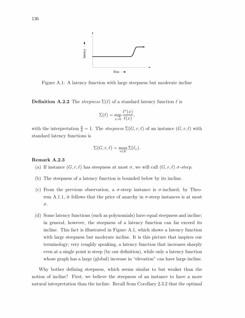
136

late

ncy

flow

Figure A.1: A latency function with large steepness but moderate incline

Definition A.2.2 The steepness Σ() of a standard latency function is

Σ() = supx>0

∗(x)

(x),

with the interpretation 00

= 1. The steepness Σ(G, r, ) of an instance (G, r, ) with

standard latency functions is

Σ(G, r, ) = maxe∈E

Σ(e).

Remark A.2.3

(a) If instance (G, r, ) has steepness at most σ, we will call (G, r, ) σ-steep.

(b) The steepness of a latency function is bounded below by its incline.

(c) From the previous observation, a σ-steep instance is σ-inclined; by Theo-

rem A.1.1, it follows that the price of anarchy in σ-steep instances is at most

σ.

(d) Some latency functions (such as polynomials) have equal steepness and incline;

in general, however, the steepness of a latency function can far exceed its

incline. This fact is illustrated in Figure A.1, which shows a latency function

with large steepness but moderate incline. It is this picture that inspires our

terminology; very roughly speaking, a latency function that increases sharply

even at a single point is steep (by our definition), while only a latency function

whose graph has a large (global) increase in “elevation” can have large incline.

Why bother defining steepness, which seems similar to but weaker than the

notion of incline? First, we believe the steepness of an instance to have a more

natural interpretation than the incline. Recall from Corollary 2.3.2 that the optimal

137

flow in a network with standard latency functions is nothing more than a flow at

Nash equilibrium with respect to the marginal cost functions ∗; thus, the steepness

of an instance simply measures the worst-case discrepancy between how a Nash

and an optimal flow evaluates the cost of increasing flow on an edge (cf., the hard-

to-interpret objective function minimized by a flow at Nash equilibrium). Second,

we will see in Section A.3 that the steepness of an instance controls the potential

“unfairness” of an optimal flow (recall the example of Subsection 2.4.5).

A.3 How Unfair is Optimal Routing?

We saw in Subsection 2.4.5 that optimal flows, while minimizing the total latency,

may lack desirable fairness properties—specifically, that some traffic in a minimum-

latency flow may be routed on paths with larger latency than that incurred by all

traffic in a Nash flow. This drawback of routing traffic optimally has inspired prac-

titioners to find traffic assignments that minimize total latency subject to explicit

length constraints [90], which require that no network users experience much more

latency than in a flow at Nash equilibrium. The question we study in this section

is the following: how much worse off can network users be in an optimal flow than

in one at Nash equilibrium?.

For the rest of this section, we will confine ourselves to instances in which all

traffic shares a common source and destination. Define the unfairness of such an

instance (G, r, ) as the maximum ratio between the latency of a flow path of an

optimal flow for (G, r, ) and that of a flow path of a Nash flow for (G, r, ). We

denote the unfairness of instance (G, r, ) by u(G, r, ).

Our first observation is that u(G, r, ) can be arbitrarily large if we do not place

additional restrictions on the class of allowable latency functions. To see this, modify

the example of Subsection 2.4.5 as follows: for any positive integer p, define the

latency of the first edge as the constant function (x) = (p + 1)(1 − ε) and that of

the second edge as (x) = xp. In this example, u(G, r, ) = (p + 1)(1 − ε), which

tends to +∞ with p.

In the spirit of our work bounding the price of anarchy, we aim to quantify the

worst possible unfairness as a function of the class of allowable latency functions.

We have already formulated the appropriate notion of “steepness” for quantifying

the unfairness of optimal flows in instances with standard latency functions in the

previous section; namely, the notion of steepness given in Definition A.2.2.

138

Theorem A.3.1 If (G, r, ) is an instance with a single source-destination pair and

standard latency functions, then

u(G, r, ) ≤ Σ(G, r, ).

Proof. Let (G, r, ) be an instance with source s, destination t, standard latency

functions, and steepness σ. Suppose f and f ∗ are Nash and optimal flows for

(G, r, ), respectively. We need to show that the maximum latency of a flow path of

f ∗ is at most σ times the latency of a flow path of f .

Suppose for contradiction that P1, P2 are paths s-t satisfying fP1 > 0, f ∗P2

> 0,

and P2(f∗) > σ · P1(f). Since f is at Nash equilibrium for (G, r, ), by Propo-

sition 2.2.2 all flow paths of f have a common latency L with respect to latency

functions . Similarly, by Corollary 2.3.2 all flow paths of f ∗ have a common latency

L∗ with respect to latency functions ∗.

Now, as every latency function is nondecreasing, we have e(x) ≤ ∗e(x) for all e

and x. Thus, we may derive

L = P1(f) <1

σP2(f

∗) ≤ 1

σ∗P2

(f ∗) =L∗

σ.

By Proposition 2.2.4, the cost of the flow f is C(f) = rL. The cost of the optimal

flow f ∗ is not so easy to compute, as flow paths have equal latency with respect to

functions ∗ but not with respect to . However, since every latency function has

steepness at most σ, we obtain ∗P (f ∗) ≤ σ · P (f ∗) for every path P and hence

C(f ∗) ≥ 1

σ

∑P∈P

∗P (f ∗)f ∗P =

1

σrL∗ > rL = C(f),

which contradicts the optimality of f ∗.

For example, an instance whose latency functions are polynomials with nonneg-

ative coefficients of degree at most p has unfairness at most p + 1.

Remark A.3.2 Theorem A.3.1 is not sharp on all instances (for a trivial case,

take G to be a single link with latency function (x) = x). However, the theorem

is best possible in the following sense: for any real number c ≥ 1, there is an

instance (G, r, ) with standard latency functions satisfying Σ(G, r, ) ≤ c (namely,

the example given at the beginning of this section with p everywhere replaced by

c − 1) with unfairness arbitrarily close to c.

139

Remark A.3.3 Theorem A.3.1 and the previous remark provide an analogue of

our work in Sections 3.3–3.4 showing that the price of anarchy is independent of

the network topology. Let L denote a standard class of latency functions includ-

ing the constant functions, and define the steepness Σ(L) by Σ(L) = sup∈L Σ().

Then sup(G,r,) u(G, r, ) (where the supremum ranges over instances with a single

source-destination pair and latency functions in L) is precisely Σ(L), with worst-case

examples furnished by networks of two parallel links. In fact, it is not difficult to see

that this statement remains true with the weaker assumptions that L is standard

and is diverse in the sense that (0) : ∈ L = (0,∞) (cf. Theorem 3.4.4, where

more than two links are required for worst-case examples of the inefficiency of Nash

flows).

A further generalization (in the spirit of Section 3.5) is the following: if L is

standard and contains a latency function that is positive when evaluated with zero

congestion, then the worst-case unfairness of optimal flows (with respect to L) is

achieved (modulo an arbitrarily small additive factor) in subdivisions of a two-node,

two-link network. Some assumption on L is necessary for this sort of result; indeed,

any network with latency functions drawn from Lp = axp : a > 0 has steepness

p + 1 but unfairness 1 (by a straightforward generalization of Corollary 3.2.2).

Appendix B

A Collection of Counterexamples

B.1 Necessity of Continuous, Nondecreasing La-

tency Functions for Nash Flows

In this section, we provide several examples demonstrating that the useful properties

of flows at Nash equilibrium presented in Chapter 2, such as existence and unique-

ness, fail if we allow edge latency functions to be discontinuous or nonmonotone.

The next two propositions study networks with latency functions that are non-

decreasing but not continuous. We first show that Nash flows need not exist in such

networks.

Proposition B.1.1 There is a network G with nondecreasing discontinuous latency

functions and a traffic rate r such that (G, r, ) fails to admit a feasible flow at

Nash equilibrium.

Proof. Let G denote a two-node two-link network. Define one latency function by

1(x) = 1 and another by

2(x) =

x if x < 1

2 if x ≥ 1.

It is evident that both latency functions are nondecreasing and that no flow feasible

for (G, 1, ) meets the definition of a Nash flow set forth in Definition 2.2.1.

The next proposition demonstrates that networks with discontinuous latency

functions can admit Nash flows with distinct costs.

140

141

Proposition B.1.2 There is a network G with nondecreasing discontinuous latency

functions and a traffic rate r such that (G, r, ) admits two feasible flows at Nash

equilibrium with different costs.

Proof. Define a network G as in the previous proposition. Define the first latency

function 1 by

1(x) =

0 if x ∈ [0, 13]

1 if x > 13

and the second by

2(x) =

12

if x ∈ [0, 13]

1 if x > 13.

Again set the traffic rate r to be 1. One flow at Nash equilibrium routes 13

of the

flow on the first edge and the rest on the second, for a cost of 23; another routes 2

3

of the the flow on the first edge and the rest on the second, for a cost of 56.

Remark B.1.3 The previous example also shows that the characterization of Nash

flows given in Proposition 2.2.2 fails when network latency functions need not be

continuous: Nash flows in such networks need not route all flow on paths having

minimum-latency.

We next consider networks in which latency functions are continuous but are not

assumed to be nondecreasing. While Nash flows still exist (as the proof of Proposi-

tion 2.5.1 shows), they are no longer unique in any sense. This is demonstrated in

the next proposition.

Proposition B.1.4 There is a network G with nonmonotone continuous latency

functions and a traffic rate r such that (G, r, ) admits two feasible flows at Nash

equilibrium with different costs.

Proof. Let G denote a network with two nodes and three parallel links. Endow

the first two links with the latency function (x) = (x − 12)2 + 1 and the third with

latency function (x) = max2 − 2x, 0. Then (G, 1, ) admits a Nash flow that

routes half the traffic on each of the first two links (for a cost of 1) and another

Nash flow that routes all traffic on the third link (for a cost of 0).

Remark B.1.5 A variant on the previous example shows that the characterization

of Nash flows given in Proposition 2.2.2 fails in networks with nonmonotone latency

functions. To see this, replace the latency function on the third edge of the network

142

ts v w0f(x)

2

f(x)

1−ε 1−ε

Figure B.1: Theorem 4.1.3 is sharp

above by the less severe latency function (x) = max1−x, 0. The flow that routes

half of the traffic on each of the first two edges equalizes the latency of all three

edges at 1 but is not at Nash equilibrium; any traffic would be better off by rerouting

itself on the third link.

B.2 Theorem 4.1.3 is Sharp

In Section 4.1 we defined the notion of a flow at ε-approximate Nash equilibrium

and showed in Theorem 4.1.3 that if f is at ε-approximate Nash equilibrium for the

instance (G, r, ) and f ∗ is feasible for (G, 2r, ), then C(f) ≤ 1+ε1−ε

C(f ∗). We now

show that the factor of 1+ε1−ε

cannot be improved in general network topologies.

Fix ε ∈ (0, 1) and consider the network G shown in Figure B.1 (with topology

identical to that of Figure 4.1, namely the Braess Paradox graph of Figure 2.2 with a

direct s-t edge added). Four of the edges have constant latency functions, as shown,

and by f(x) we mean a nondecreasing, continuous function equal to 0 on [0, 1 − δ]

and to 1 + ε on [1,∞) (where δ > 0 is arbitrarily small). The flow f routing 1 unit

of flow on the three-hop path s → v → w → t is at ε-approximate Nash equilibrium

for (G, 1, ) and has cost 2(1+ ε). On the other hand, the flow f ∗ routing 1−δ units

of flow on each of the two-hop paths and 2δ units of flow on the s-t edge is feasible

and has cost approaching 2(1 − ε) as δ → 0.

On the other hand, the factor of 1+ε1−ε

can be improved to 1 + ε in networks of

parallel links.

Proposition B.2.1 Let G be a network of parallel links and f at ε-approximate

Nash equilibrium for (G, r, ). If f ∗ is feasible for (G, 2r, ), then C(f) ≤ (1 +

ε)C(f ∗).

143

Proof. Let L be the minimum latency of any edge with respect to f ; since G is

a network of parallel links and f is at ε-approximate Nash equilibrium, we have

C(f) ≤ (1 + ε)rL. Let E1 be the edges e of G for which f ∗e < fe, and E2 the rest of

the edges. Since G is a network of parallel links, f ∗ routes less than∑

e∈E1fe ≤ r

units of flow on edges in E1. Thus, f ∗ routes at least 2r − r = r units of flow on

edges of E2. Since f ∗e ≥ fe for all edges e ∈ E2, we have e(f

∗e ) ≥ e(fe) ≥ L for

all e ∈ E2. We have shown that at least r units of f ∗ experience at least L units of

latency; hence C(f ∗) ≥ rL ≥ C(f)1+ε

.

B.3 Stackelberg Routing in General Networks

In Section 6.4, we proved that in networks of parallel links a carefully chosen Stack-

elberg strategy induces a flow with cost no more than 1β

times that of the minimum-

latency flow, where β is the fraction of the traffic that is centrally controlled. In this

section we show that this guarantee cannot be extended to more general network

topologies. Specifically, we have the following bad example in the graph of Braess’s

Paradox (Figure 2.2).

Proposition B.3.1 There is a Stackelberg instance (G, r, , β) in which no flow

induced by a Stackelberg strategy has cost at most C(f ∗)/β, where f ∗ is an optimal

flow for (G, r, ).

Proof. Let G be the graph of Braess’s Paradox (see Figure B.2). Let the latency

functions of edges (s, w) and (v, t) be (x) = 1 and of (v, w) be (x) = 0 (as

in Braess’s Paradox). Define the latency function of the remaining two edges by

(x) = f(x), where f(x) = 0 on [0, 34−ε], f(x) = 1−ε on [3

4,∞), and f(x) is defined

arbitrarily on (34−ε, 3

4) subject to the usual continuity and monotonicity restrictions

(where ε > 0 is arbitrarily small). The flow feasible for (G, 1, ) routing 12− 2ε units

of flow on the three-hop path and 14

+ ε units of flow on each of the two-hop paths

has cost approaching 12

as ε → 0.

Now consider the Stackelberg instance (G, 1, , 12), and any Stackelberg strategy

f . We must show that the flow induced by f has large cost. We first observe

that, for any strategy f , all selfish traffic will be routed on the three-hop path

s → v → w → t. All that remains is a simple case analysis.

Case 1: Suppose f routes at least 14

units of flow both on edge (s, v) and on edge

(w, t). By the previous observation, the flow induced by f routes at least 34

units of

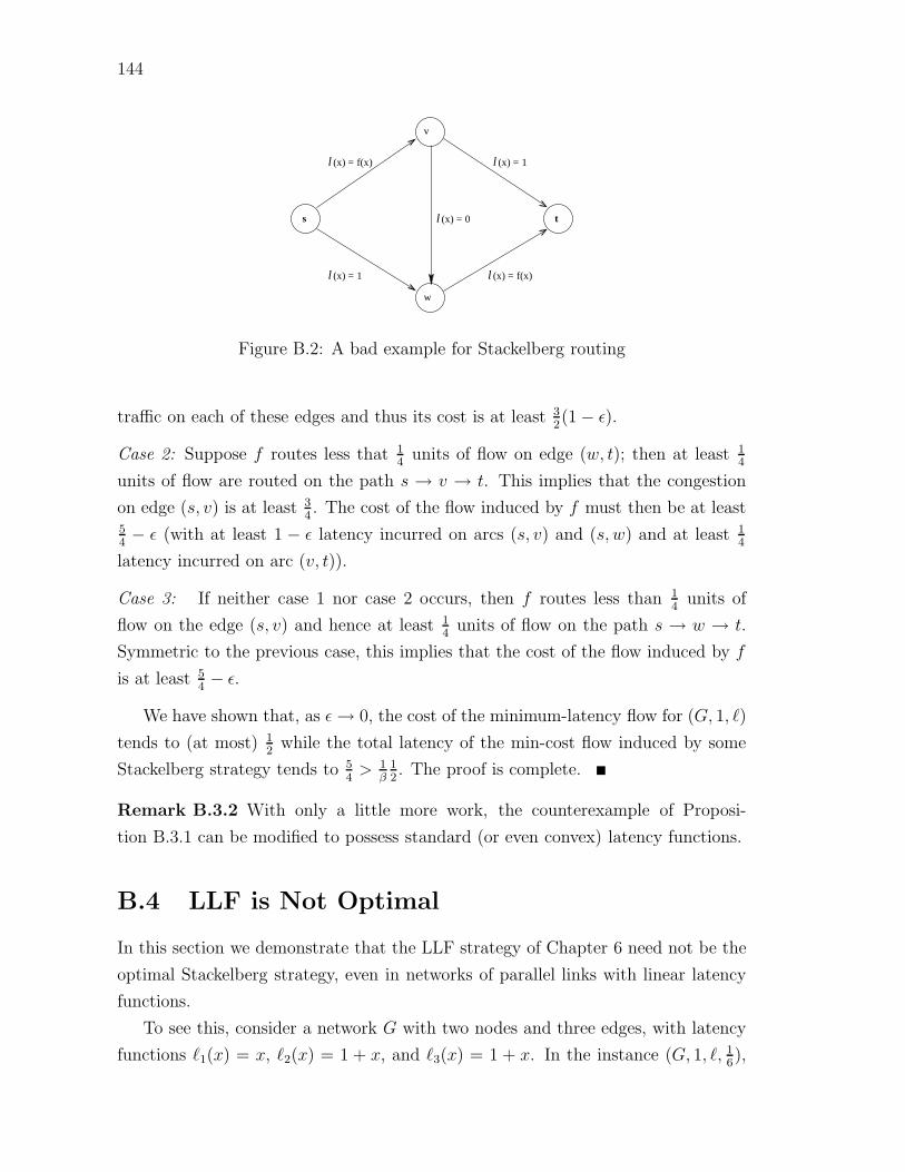
144

l (x) = f(x) l (x) = 1

s t

w

v

l (x) = 1

l (x) = 0

l (x) = f(x)

Figure B.2: A bad example for Stackelberg routing

traffic on each of these edges and thus its cost is at least 32(1 − ε).

Case 2: Suppose f routes less that 14

units of flow on edge (w, t); then at least 14

units of flow are routed on the path s → v → t. This implies that the congestion

on edge (s, v) is at least 34. The cost of the flow induced by f must then be at least

54− ε (with at least 1 − ε latency incurred on arcs (s, v) and (s, w) and at least 1

4

latency incurred on arc (v, t)).

Case 3: If neither case 1 nor case 2 occurs, then f routes less than 14

units of

flow on the edge (s, v) and hence at least 14

units of flow on the path s → w → t.

Symmetric to the previous case, this implies that the cost of the flow induced by f

is at least 54− ε.

We have shown that, as ε → 0, the cost of the minimum-latency flow for (G, 1, )

tends to (at most) 12

while the total latency of the min-cost flow induced by some

Stackelberg strategy tends to 54

> 1β

12. The proof is complete.

Remark B.3.2 With only a little more work, the counterexample of Proposi-

tion B.3.1 can be modified to possess standard (or even convex) latency functions.

B.4 LLF is Not Optimal

In this section we demonstrate that the LLF strategy of Chapter 6 need not be the

optimal Stackelberg strategy, even in networks of parallel links with linear latency

functions.

To see this, consider a network G with two nodes and three edges, with latency

functions 1(x) = x, 2(x) = 1 + x, and 3(x) = 1 + x. In the instance (G, 1, , 16),

145

the optimal flow routes 23

of the traffic on the first edge and splits the remaining

traffic equally between the last two edges. The LLF strategy thus routes the 16

units

of centrally controlled flow on the third edge, inducing a flow with 56

of the flow on

the first edge and the rest on the third, for a cost of 89. On the other hand, the

Stackelberg strategy that routes 112

units of flow on each of last two edges induces a

flow with cost 78.

Bibliography

[1] H. Z. Aashtiani and T. L. Magnanti. Equilibria on a congested transportationnetwork. SIAM Journal on Algebraic and Discrete Methods, 2(3):213–226,1981.

[2] A. V. Aho, J. E. Hopcroft, and J. D. Ullman. The Design and Analysis ofComputer Algorithms. Addison-Wesley, 1974.

[3] R. K. Ahuja, T. L. Magnanti, and J. B. Orlin. Network Flows: Theory,Algorithms, and Applications. Prentice-Hall, 1993.

[4] E. Altman, T. Basar, T. Jimenez, and N. Shimkin. Competitive routing innetworks with polynomial costs. In Proceedings of INFOCOM, volume 3, pages1586–1593, 2000.

[5] E. Altman, T. Basar, T. Jimenez, and N. Shimkin. Routing into two par-allel links: Game-theoretic distributed algorithms. Journal of Parallel andDistributed Computing, 61(9):1367–1381, 2001.

[6] E. Altman, T. Boulogne, R. El Azouzi, and T. Jimenez. A survey on network-ing games in telecommunications. Manuscript, 2000.

[7] E. Altman, R. El Azouzi, and O. Pourtallier. Avoiding paradoxes in routinggames. In Proceedings of the 17th International Teletraffic Conference, 2001.

[8] E. Altman and H. Kameda. Equilibria for multiclass routing in multi-agentnetworks. In Proceedings of the 40th Annual IEEE Conference on Decisionand Control, 2001.

[9] R. Arnott, A. De Palma, and R. Lindsey. Properties of dynamic traffic equilib-rium involving bottlenecks, including a paradox and metering. TransportationScience, 27(2):148–160, 1993.

[10] R. Arnott and K. Small. The economics of traffic congestion. AmericanScientist, 82(5):446–455, 1994.

[11] R. Asmuth, B. C. Eaves, and E. L. Peterson. Computing economic equilib-ria on affine networks with Lemke’s algorithm. Mathematics of OperationsResearch, 4(3):209–214, 1979.

146

147

[12] A. Bagchi. Stackelberg Differential Games in Economic Models. Springer-Verlag, 1984.

[13] T. Basar and G. J. Olsder. Dynamic Noncooperative Game Theory. SIAM,1999.

[14] T. Bass. Road to ruin. Discover, 13:56–61, 1992.

[15] N. Bean. Secrets of network success. Physics World, pages 30–33, February1996.

[16] N. G. Bean, F. P. Kelly, and P. G. Taylor. Braess’s paradox in a loss network.Journal of Applied Probability, 34:155–159, 1997.

[17] M. Beckmann, C. B. McGuire, and C. B. Winsten. Studies in the Economicsof Transportation. Yale University Press, 1956.

[18] L. D. Bennett. The existence of equivalent mathematical programs for certainmixed equilibrium traffic assignment problems. European Journal of Opera-tional Research, 72:177–187, 1993.

[19] D. P. Bertsekas. Network Optimization: Continuous and Discrete Models.Athena Scientific, 1998.

[20] D. P. Bertsekas and R. Gallager. Data Networks. Prentice-Hall, 1992. SecondEdition.

[21] K. P. Birman. Building Secure and Reliable Network Applications. Manning,1996.

[22] M. Blonski. Anonymous games with binary actions. Games and EconomicBehavior, 28:171–180, 1999.

[23] B. Bollobas. Random Graphs. Academic Press, 1985.

[24] R. Bott and R. J. Duffin. On the algebra of networks. Transactions of theAMS, 74:99–109, 1953.

[25] T. Boulogne and E. Altman. Competitive routing in multicast communica-tions. Manuscript, 2001.

[26] T. Boulogne, E. Altman, H. Kameda, and O. Pourtallier. Mixed equilibriumfor multiclass routing games. In Proceedings of the 9th International Sympo-sium on Dynamic Games and Applications, pages 58–74, 2000.

[27] D. E. Boyce and J. L. Soberanes. Solutions to the optimal network designproblem with shipments related to transportation cost. Transportation Re-search, 13B(1):65–80, 1979.

148

[28] D. Braess. Uber ein paradoxon der verkehrsplanung. Unternehmensforschung,12:258–268, 1968. Available from http://homepage.ruhr-uni-bochum.de/

Dietrich.Braess/.

[29] B. Calvert. The Downs-Thomson effect in a Markov process. Probability inthe Engineering and Informational Sciences, 11:327–340, 1997.

[30] B. Calvert and G. Keady. Braess’s paradox and power-law nonlinearities innetworks. Journal of the Australian Mathematical Society, Series B, 35:1–22,1993.

[31] B. Calvert, W. Solomon, and I. Ziedins. Braess’s paradox in a queueing net-work with state-dependent routing. Journal of Applied Probability, 34:134–154,1997.

[32] M. Carey. Optimal time-varying flows on congested networks. OperationsResearch, 35(1):58–69, 1987.

[33] S. Catoni and S. Pallottino. Traffic equilibrium paradoxes. TransportationScience, 25(3):240–244, 1991.

[34] V. Chvatal. Linear Programming. Freeman, 1983.

[35] J. E. Cohen. The counterintuitive in conflict and cooperation. AmericanScientist, 76:577–584, 1988.

[36] J. E. Cohen and P. Horowitz. Paradoxical behavior of mechanical and electricalnetworks. Nature, 352:699–701, 1991.

[37] J. E. Cohen and C. Jeffries. Congestion resulting from increased capacity insingle-server queueing networks. IEEE/ACM Transactions on Communica-tion, 5(2):305–310, 1997.

[38] J. E. Cohen and F. P. Kelly. A paradox of congestion in a queuing network.Journal of Applied Probability, 27:730–734, 1990.

[39] R. M. Cohn. The resistance of an electrical network. Proceedings of the AMS,1:316–324, 1950.

[40] R. W. Cottle, J. Pang, and R. E. Stone. The Linear Complementarity Problem.Academic Press, 1992.

[41] J. B. Cruz, Jr. Leader-follower strategies for multilevel systems. IEEE Trans-actions on Automatic Control, AC-23(2):244–255, 1978.

[42] J. B. Cruz, Jr. Survey of leader-follower concepts in hierarchical decision-making. In Proceedings of the 4th Annual International Conference on theAnalysis and Optimization of Systems, pages 384–396, 1980.

149

[43] A. Czumaj, P. Krysta, and B. Vocking. Selfish traffic allocation for serverfarms. In Proceedings of the 34th Annual ACM Symposium on the Theory ofComputing, 2002. To appear.

[44] A. Czumaj and B. Vocking. Tight bounds for worst-case equilibria. In Proceed-ings of the 13th Annual Symposium on Discrete Algorithms, pages 413–420,2002.

[45] S. C. Dafermos. An extended traffic assignment model with applications totwo-way traffic. Transportation Science, 5:366–389, 1971.

[46] S. C. Dafermos. The traffic assignment problem for multiclass-user transporta-tion networks. Transportation Science, 6:73–87, 1972.

[47] S. C. Dafermos. Traffic equilibrium and variational inequalities. Transporta-tion Science, 14(1):42–54, 1980.

[48] S. C. Dafermos and A. Nagurney. On some traffic equilibrium theory para-doxes. Transportation Research, Series B, 18B:101–110, 1984.

[49] S. C. Dafermos and A. Nagurney. Sensitivity analysis for the asymmetricnetwork equilibrium problem. Mathematical Programming, 28:174–184, 1984.

[50] S. C. Dafermos and F. T. Sparrow. The traffic assignment problem for ageneral network. Journal of Research of the National Bureau of Standards,Series B, 73B(2):91–118, 1969.

[51] C. F. Daganzo. Queue spillovers in transportation networks with a routechoice. Transportation Science, 32(1):3–11, 1998.

[52] R. Dionne and M. Florian. Exact and approximate algorithms for optimalnetwork design. Networks, 9(1):37–59, 1979.

[53] C. Douligeris and R. Mazumdar. Multilevel flow control of queues. In Proceed-ings of the Johns Hopkins Conference on Information Sciences and Systems,page 21, 1989.

[54] C. Douligeris and R. Mazumdar. A game theoretic perspective to flow controlin telecommunication networks. Journal of the Franklin Institute, 329:383–402,1992.

[55] A. Downs. The law of peak-hour expressway congestion. Traffic Quarterly,16:393–409, 1962.

[56] P. Dubey. Inefficiency of Nash equilibria. Mathematics of Operations Research,11(1):1–8, 1986.

[57] R. J. Duffin. Topology of series-parallel networks. Journal of MathematicalAnalysis and Applications, 10:303–318, 1965.

150

[58] A. A. Economides and J. A. Silvester. Priority load sharing: An approach us-ing Stackelberg games. In Proceedings of the 28th Annual Allerton Conferenceon Communications, Control, and Computing, pages 674–683, 1990.

[59] R. El Azouzi and E. Altman. Side constrained traffic equilibrium in multiusercommunication networks. In Allerton Conference on Communication, Control,and Computing, 2001.

[60] R. El Azouzi, E. Altman, and O. Pourtallier. Properties of equilibria in com-petitive routing with several user types. Manuscript, 2001.

[61] P. Erdos and A. Renyi. On the evolution of random graphs. Publ. Math. Inst.Hungar. Acad. Sci., 5:17–61, 1960.

[62] G. Facchini, F. van Megan, P. Borm, and S. Tijs. Congestion models andweighted Bayesian potential games. Theory and Decision, 42:193–206, 1997.

[63] C. Fisk. More paradoxes in the equilibrium assignment problem. Transporta-tion Research, 13B:305–309, 1979.

[64] C. Fisk and S. Pallottino. Empirical evidence for equilibrium paradoxes withimplications for optimal planning strategies. Transportation Research, SeriesA, 15:245–248, 1981.

[65] M. Florian. A traffic equilibrium model of travel by car and public transitmodes. Transportation Science, 11(2):166–179, 1977.

[66] M. Florian. An introduction to network models used in transportation plan-ning. In M. Florian, editor, Transportation Planning Models, pages 137–152.Elsevier Science, 1984.

[67] M. Florian. Nonlinear cost network models in transportation analysis. Math-ematical Programming Study, 26:167–196, 1986.

[68] M. Florian and D. Hearn. Network equilibrium models and algorithms. InM. O. Ball, T. Magnanti, C. Monma, and G. Nemhauser, editors, NetworkRouting, chapter 6, pages 485–550. Elsevier Science, 1995.

[69] M. Florian and S. Nguyen. A method for computing network equilibrium withelastic demands. Transportation Science, 8:321–332, 1974.

[70] S. Fortune, J. E. Hopcroft, and J. Wyllie. The directed subgraph homeomor-phism problem. Theoretical Computer Science, 10:111–121, 1980.

[71] M. Frank. The Braess Paradox. Mathematical Programming, 20:283–302,1981.

[72] M. Frank. Cost-deceptive links on ladder networks. Methods of OperationsResearch, 45:75–86, 1983.

151

[73] E. J. Friedman. Dynamics and rationality in ordered externality games. Gamesand Economic Behavior, 16:65–76, 1996.

[74] E. J. Friedman. A generic analysis of selfish routing. Working paper. Availablefrom http://www.orie.cornell.edu/~friedman/papers.htm, 2001.

[75] D. Fudenberg and J. Tirole. Game Theory. MIT Press, 1991.

[76] C. B. Garcia and W. I. Zangwill. Pathways to Solutions, Fixed Points, andEquilibria. Prentice-Hall, 1981.

[77] M. R. Garey and D. S. Johnson. Computers and Intractability: A Guide tothe Theory of NP-Completeness. Freeman, 1979.

[78] C. Gawron. An iterative algorithm to determine the dynamic user equilibriumin a traffic simulation model. International Journal of Modern Physics C,9(3):393–407, 1998.

[79] M. X. Goemans and D. P. Williamson. The primal-dual method for approx-imation algorithms and its application to network design problems. In D. S.Hochbaum, editor, Approximation Algorithms for NP-Hard Problems, chap-ter 4, pages 144–191. PWS Publishing Company, 1997.

[80] D. Gross and C. M. Harris. Queueing Theory. Wiley, 1998. Third Edition.

[81] M. Grotschel, L. Lovasz, and A. Schrijver. Geometric Algorithms and Combi-natorial Optimization. Springer-Verlag, 1993. Second corrected edition.

[82] J. N. Hagstrom and R. A. Abrams. Characterizing Braess’s paradox for trafficnetworks. In IEEE Conference on Intelligent Transportation Systems, pages837–842, 2001.

[83] M. A. Hall. Properties of the equilibrium state in transportation networks.Transportation Science, 12(3):208–216, 1978.

[84] A. Haurie and P. Marcotte. On the relationship between Nash-Cournot andWardrop equilibria. Networks, 15:295–308, 1985.

[85] A. Haurie and P. Marcotte. A game-theoretic approach to network equilibrium.Mathematical Programming Study, 26:252–255, 1986.

[86] H. H. Hoc. A computational approach to the selection of an optimal network.Management Science, 19(5):488–498, 1973.

[87] D. S. Hochbaum and J. G. Shanthikumar. Convex separable optimization isnot much harder than linear optimization. Journal of the ACM, 37(4):843–862,1990.

152

[88] R. Holzman and N. Law-Yone. Strong equilibrium in congestion games. Gamesand Economic Behavior, 21:85–101, 1997.

[89] A. D. Irvine. How Braess’ paradox solves Newcomb’s problem. InternationalStudies in the Philosophy of Science, 7(2):141–160, 1993.

[90] O. Jahn, R. Mohring, and A. S. Schulz. Optimal routing of traffic flowswith length restrictions in networks with congestion. In Operations ResearchProceedings 1999, pages 437–442, 2000.

[91] B. Kalyanasundaram and K. Pruhs. Speed is as powerful as clairvoyance.Journal of the ACM, 47(4):617–643, 2000. Preliminary version in FOCS ’95.

[92] H. Kameda, E. Altman, T. Kozawa, and Y. Hosokawa. Braess-like paradoxesin distributed computer systems. IEEE Transactions on Automatic Control,45(9):1687–1691, 2000.

[93] H. Kameda, E. Altman, J. Li, and Y. Hosokawa. Paradoxes in performanceoptimization of distributed systems. In International Conference on Advancesin Infrastructure for Electronic Business, Science, and Education on the In-ternet, 2000.

[94] S. Karlin and H. M. Taylor. A Second Course in Stochastic Processes. Aca-demic Press, 1981.

[95] R. M. Karp. Reducibility among combinatorial problems. In R. E. Millerand J. W. Thatcher, editors, Complexity of Computer Computations, pages85–103. Plenum Press, 1972.

[96] G. Keady. The Colebrook-White formula for pipe networks. Electronic report,Department of Mathematics, University of Western Australia, 1995.

[97] F. P. Kelly. Network routing. Philosophical Transactions of the Royal Societyof London, Series A, 337:343–367, 1991.

[98] S. Keshav. An Engineering Approach to Computer Networking. Addison-Wesley, 1997.

[99] F. H. Knight. Some fallacies in the interpretation of social cost. QuarterlyJournal of Economics, 38:582–606, 1924.

[100] W. Knodel. Graphentheoretische Methoden und ihre Anwendungen. Springer-Verlag, 1969.

[101] G. Kolata. What if they closed 42nd Street and nobody noticed? New YorkTimes, page 38, December 25 1990.

153

[102] H. Konishi. Uniqueness of user equilibrium in transportation networks withheterogeneous commuters. Working paper, Department of Economics, BostonCollege, 2001.

[103] H. Konishi, M. Le Breton, and S. Weber. Equilibria in a model with partialrivalry. Journal of Economic Theory, 72:225–237, 1997.

[104] Y. A. Korilis, A. A. Lazar, and A. Orda. Achieving network optima us-ing Stackelberg routing strategies. IEEE/ACM Transactions on Networking,5(1):161–173, 1997.

[105] Y. A. Korilis, A. A. Lazar, and A. Orda. Capacity allocation under nonco-operative routing. IEEE Transactions on Automatic Control, 42(3):309–325,1997.

[106] Y. A. Korilis, A. A. Lazar, and A. Orda. Avoiding the Braess paradox innoncooperative networks. Journal of Applied Probability, 36(1):211–222, 1999.

[107] T. W. Korner. The Pleasures of Counting. Cambridge University Press, 1996.

[108] E. Koutsoupias and C. H. Papadimitriou. Worst-case equilibria. In Proceedingsof the 16th Annual Symposium on Theoretical Aspects of Computer Science,pages 404–413, 1999.

[109] D. C. Kozen. Design and Analysis of Algorithms. Springer-Verlag, 1992.

[110] N. S. Kukushkin. Potential games: A purely ordinal approach. EconomicsLetters, 34:279–283, 1999.

[111] N. S. Kukushkin. Perfect information and potential games. Games and Eco-nomic Behavior, 38:306–317, 2002.

[112] V. S. A. Kumar and M. V. Marathe. Improved results for Stackelberg schedul-ing strategies. Manuscript, 2002.

[113] A. A. Lazar, A. Orda, and D. E. Pendarakis. Virtual path bandwidth alloca-tion in multiuser networks. IEEE/ACM Transactions on Networking, 5:861–871, 1997.

[114] L. J. LeBlanc. An algorithm for the discrete network design problem. Trans-portation Research, 9:183–199, 1975.

[115] T. Leventhal, G. Nemhauser, and L. Trotter, Jr. A column generation al-gorithm for optimal traffic assignment. Transportation Science, 7:168–176,1973.

[116] L. Libman and A. Orda. The designer’s perspective to atomic noncooperativenetworks. IEEE/ACM Transactions on Networking, 7(6):875–884, 1999.

154

[117] L. Libman and A. Orda. Atomic resource sharing in noncooperative networks.Telecommunication Systems, 17(4):385–409, 2001. Preliminary version in IN-FOCOM ’97.

[118] T. L. Magnanti. Models and algorithms for predicting urban traffic equilibria.In M. Florian, editor, Transportation Planning Models, pages 153–185. ElsevierScience, 1984.

[119] T. L. Magnanti and R. T. Wong. Network design and transportation planning:Models and algorithms. Transportation Science, 18(1):1–55, 1984.

[120] L. Marinoff. How Braess’ paradox solves Newcomb’s problem: not! Interna-tional Studies in the Philosophy of Science, 10(3):217–237, 1996.

[121] A. Mas-Colell. On a theorem of Schmeidler. Journal of Mathematical Eco-nomics, 13:201–206, 1984.

[122] M. Mavronicolas and P. Spirakis. The price of selfish routing. In Proceedingsof the 33rd Annual ACM Symposium on the Theory of Computing, pages 510–519, 2001.

[123] I. Milchtaich. Congestion games with player-specific payoff functions. Gamesand Economic Behavior, 13:111–124, 1996.

[124] I. Milchtaich. Congestion models of competition. American Naturalist,147(5):760–783, 1996.

[125] I. Milchtaich. Network topology and the efficiency of equilibrium. Workingpaper 12-01, Department of Economics, Bar-Ilan University, Israel, 2001.

[126] I. Milchtaich. Social optimality and cooperation in large congestion games.Manuscript, 2001.

[127] D. Monderer and L. S. Shapley. Potential games. Games and EconomicBehavior, 14:124–143, 1996.

[128] J. D. Murchland. Braess’s paradox of traffic flow. Transportation Research,4:391–394, 1970.

[129] A. Nagurney. Sustainable Transportation Networks. Edward Elgar, 2000.

[130] J. F. Nash, Jr. Non-cooperative games. Annals of Mathematics, 54(2):286–295,1951.

[131] Y. Nesterov. Stable flows in transportation networks. CORE Discussion Paper9907, 1999.

[132] Y. Nesterov and A. De Palma. Stable dynamics in transportation systems.CORE Discussion Paper 00/27, 2000.

155

[133] G. F. Newell. Traffic Flow on Transportation Networks. MIT Press, 1980.

[134] S. Nguyen. An algorithm for the traffic assignment problem. TransportationScience, 8:203–216, 1974.

[135] S. Nguyen and C. Dupuis. An efficient method for computing traffic equilibriain networks with asymmetric transportation costs. Transportation Science,18(2):185–202, 1984.

[136] N. Nisan. Algorithms for selfish agents: Mechanism design for distributedcomputation. In Proceedings of the 16th Annual Symposium on TheoreticalAspects of Computer Science, pages 1–15, 1999.

[137] N. Nisan and A. Ronen. Algorithmic mechanism design. Games and EconomicBehavior, 35(1/2):166–196, 2001. Preliminary version in STOC ’99.

[138] A. Orda, R. Rom, and N. Shimkin. Competitive routing in multi-user com-munication networks. IEEE/ACM Transactions on Networking, 1:510–521,1993.

[139] M. J. Osbourne and A. Rubinstein. A Course in Game Theory. MIT Press,1994.

[140] G. Owen. Game Theory. Academic Press, 1995. Third Edition.

[141] C. H. Papadimitriou. Computational Complexity. Addison-Wesley, 1994.

[142] C. H. Papadimitriou. Algorithms, games, and the Internet. In Proceedings ofthe 33rd Annual ACM Symposium on the Theory of Computing, pages 749–753, 2001.

[143] E. I. Pas and S. L. Principio. Braess’ paradox: Some new insights. Trans-portation Research, Series B, 31(3):265–276, 1997.

[144] C. M. Penchina. Braess paradox: Maximum penalty in a minimal criticalnetwork. Transportation Research, Series A, 31(5):379–388, 1997.

[145] A. L. Peressini, F. E. Sullivan, and J. J. Uhl. The Mathematics of NonlinearProgramming. Springer-Verlag, 1988.

[146] I. Peterson. Strings and springs net mechanical surprise. Science News,140(8):118, August 1991.

[147] C. A. Phillips, C. Stein, E. Torng, and J. Wein. Optimal time-critical schedul-ing via resource augmentation. Algorithmica, 32(2):163–200, 2002. Preliminaryversion in STOC ’97.

[148] A. C. Pigou. The economics of welfare. Macmillan, 1920.

156

[149] T. Quint and M. Shubik. A model of migration. Working paper, CowlesFoundation, Yale University, 1994.

[150] A. Rapoport and A. Chammah. Prisoner’s Dilemma. University of MichiganPress, 1965.

[151] K. P. Rath. A direct proof of the existence of pure strategy equilibria in gameswith a continuum of players. Economic Theory, 2:427–433, 1992.

[152] J. Renegar. A Mathematical View of Interior-Point Methods in Convex Opti-mization. SIAM, 2001.

[153] C. ReVelle and D. Serra. The maximum capture problem including relocation.INFOR, 29:130–138, 1991.

[154] T. M. Ridley. An investment policy to reduce the travel time in a transporta-tion network. Transportation Research, 2(4):409–424, 1968.

[155] A. Ronen. Algorithms for rational agents. In Conference on Current Trendsin Theory and Practice of Informatics, pages 56–70, 2000.

[156] J. B. Rosen. Existence and uniqueness of equilibrium points for concave N -person games. Econometrica, 33(3):520–534, 1965.

[157] R. W. Rosenthal. A class of games possessing pure-strategy Nash equilibria.International Journal of Game Theory, 2:65–67, 1973.

[158] R. W. Rosenthal. The network equilibrium problem in integers. Networks,3:53–59, 1973.

[159] T. Roughgarden. Designing networks for selfish users is hard. In Proceedingsof the 42nd Annual Symposium on Foundations of Computer Science, pages472–481, 2001.

[160] T. Roughgarden. The price of anarchy in networks with polynomial edgelatency. Technical Report TR2001-1847, Cornell University, 2001.

[161] T. Roughgarden. Stackelberg scheduling strategies. In Proceedings of the 33rdAnnual ACM Symposium on the Theory of Computing, pages 104–113, 2001.

[162] T. Roughgarden. How unfair is optimal routing? In Proceedings of the 13thAnnual Symposium on Discrete Algorithms, pages 203–204, 2002.

[163] T. Roughgarden. The price of anarchy is independent of the network topol-ogy. In Proceedings of the 34th Annual ACM Symposium on the Theory ofComputing, 2002. To appear.

[164] T. Roughgarden and E. Tardos. Bounding the inefficiency of equilibria innonatomic congestion games. Manuscript, 2002.

157

[165] T. Roughgarden and E. Tardos. How bad is selfish routing? Journal of theACM, 49(2):236–259, 2002. Preliminary version in FOCS ’00.

[166] D. Schmeidler. Equilibrium points of nonatomic games. Journal of StatisticalPhysics, 7(4):295–300, 1973.

[167] A. S. Schulz and N. Stier Moses. Performance of user equilibria in trafficnetworks. Manuscript, 2001.

[168] A. J. Scott. The optimal network problem: Some computational procedures.Transportation Research, 3(2):201–210, 1969.

[169] Y. Sheffi. Urban Transportation Networks: Equilibrium Analysis with Mathe-matical Programming Methods. Prentice-Hall, 1985.

[170] S. J. Shenker. Making greed work in networks: A game-theoretic analysis ofswitch service disciplines. IEEE/ACM Transactions on Networking, 3(6):819–831, 1995.

[171] S. J. Shenker, D. Clark, D. Estrin, and S. Herzog. Pricing in computer net-works: Reshaping the research agenda. ACM Computer Communication Re-view, 26:19–43, April 1996.

[172] M. J. Smith. In a road network, increasing delay locally can reduce delayglobally. Transportation Research, 12:419–422, 1978.

[173] M. J. Smith. The existence, uniqueness and stability of traffic equilibria.Transportation Research, 13B:295–304, 1979.

[174] D. J. Songhurst, editor. Charging Communication Networks. Elsevier Science,1999.

[175] R. Steinberg and R. E. Stone. The prevalence of paradoxes in transportationequilibrium problems. Transportation Science, 22(4):231–241, 1988.

[176] R. Steinberg and W. I. Zangwill. The prevalence of Braess’ paradox. Trans-portation Science, 17(3):301–318, 1983.

[177] P. D. Straffin. Game Theory and Strategy. Mathematical Association of Amer-ica, 1993.

[178] A. Taguchi. Braess’ paradox in a two-terminal transportation network. Journalof the Operations Research Society of Japan, 25(4):376–388, 1982.

[179] R. E. Tarjan. Data Structures and Network Algorithms. SIAM, 1983.

[180] J. M. Thomson. Great Cities and Their Traffic. Gollancz, 1977.

[181] T. Ui. A Shapley value representation of potential games. Games and Eco-nomic Behavior, 31:121–135, 2000.

158

[182] J. Valdes, R. E. Tarjan, and E. L. Lawler. The recognition of series paralleldigraphs. SIAM Journal on Computing, 11(2):298–313, 1982.

[183] A. Vetta. Nash equilibria in competitive societies, with applications to facilitylocation, traffic routing and auctions. Manuscript, 2002.

[184] H. von Stackelberg. Marktform und Gleichgewicht. Springer-Verlag, 1934.English translation, entitled The Theory of the Market Economy, published in1952 by Oxford University Press.

[185] M. Voorneveld, P. Borm, F. van Megan, S. Tijs, and G. Facchini. Congestiongames and potentials reconsidered. International Game Theory Review, 1:283–299, 1999.

[186] J. G. Wardrop. Some theoretical aspects of road traffic research. In Proceedingsof the Institute of Civil Engineers, Pt. II, volume 1, pages 325–378, 1952.

[187] A. Weintraub and J. Gonzalez. An algorithm for the traffic assignment prob-lem. Networks, 10:197–209, 1980.

[188] W. Whitt. Counterexamples for comparisons of queues with finite waitingrooms. Queueing Systems, 10:271–278, 1992.

[189] R. T. Wong. Introduction and recent advances in network design: Modelsand algorithms. In M. Florian, editor, Transportation Planning Models, pages187–225. Elsevier Science, 1984.

[190] H. Yang. Sensitivity analysis for the elastic-demand network equilibrium prob-lem with applications. Transportation Research, Series B, 31(1):55–70, 1997.

[191] H. Yang and M. G. H. Bell. A capacity paradox in network design and howto avoid it. Transportation Research, Series A, 32(7):539–545, 1998.

[192] W. I. Zangwill and C. B. Garcia. Equilibrium programming: The path follow-ing approach and dynamics. Mathematical Programming, 21:262–289, 1981.