Self-study manual for introduction to computational fluid

Self-study manual for introduction to computational fluid

dynamics

Bachelor’s thesis

Riihimäki, Mechanical Engineering and Production Technology

Spring 2017

Andrey Nabatov

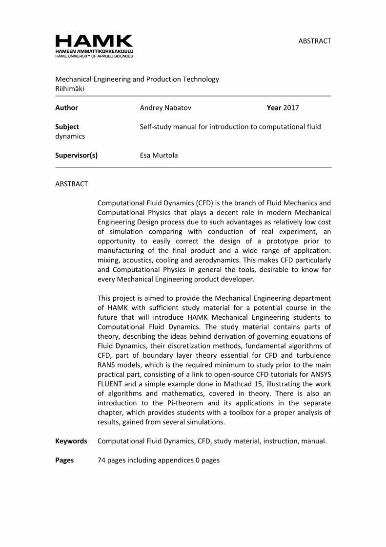
ABSTRACT Mechanical Engineering and Production Technology Riihimäki Author Andrey Nabatov Year 2017 Subject Self-study manual for introduction to computational fluid dynamics Supervisor(s) Esa Murtola ABSTRACT

Computational Fluid Dynamics (CFD) is the branch of Fluid Mechanics and Computational Physics that plays a decent role in modern Mechanical Engineering Design process due to such advantages as relatively low cost of simulation comparing with conduction of real experiment, an opportunity to easily correct the design of a prototype prior to manufacturing of the final product and a wide range of application: mixing, acoustics, cooling and aerodynamics. This makes CFD particularly and Computational Physics in general the tools, desirable to know for every Mechanical Engineering product developer. This project is aimed to provide the Mechanical Engineering department of HAMK with sufficient study material for a potential course in the future that will introduce HAMK Mechanical Engineering students to Computational Fluid Dynamics. The study material contains parts of theory, describing the ideas behind derivation of governing equations of Fluid Dynamics, their discretization methods, fundamental algorithms of CFD, part of boundary layer theory essential for CFD and turbulence RANS models, which is the required minimum to study prior to the main practical part, consisting of a link to open-source CFD tutorials for ANSYS FLUENT and a simple example done in Mathcad 15, illustrating the work of algorithms and mathematics, covered in theory. There is also an introduction to the Pi-theorem and its applications in the separate chapter, which provides students with a toolbox for a proper analysis of results, gained from several simulations.

Keywords Computational Fluid Dynamics, CFD, study material, instruction, manual. Pages 74 pages including appendices 0 pages

CONTENTS

1 INTRODUCTION ........................................................................................................... 1

2 THEORY ........................................................................................................................ 2

2.1 Lagrangian versus Eularian approach ................................................................. 2

2.2 Governing equations. .......................................................................................... 4

2.3 Turbulence ........................................................................................................ 15

2.3.1 The law of the wall ................................................................................ 20

2.3.2 Introduction to RANS models ................................................................ 23

2.3.3 Mixing length model .............................................................................. 27

2.3.4 k-ε model ............................................................................................... 28

2.3.5 Spalart-Allmaras turbulence model ...................................................... 32

2.3.6 Reynolds stress equation models (RSM) ............................................... 34

2.3.7 Direct Numerical Simulation (DNS) and Large Eddy Simulation (LES) .. 36

2.4 Finite volume method and solution schemes ................................................... 39

2.4.1 Finite volume method for diffusion problems ...................................... 39

2.4.2 Convection-diffusion problems ............................................................. 45

2.4.3 Pressure-velocity coupling..................................................................... 49

3 EXAMPLE SOLVED IN MATHCAD 15 .......................................................................... 57

3.1 Problem specification ........................................................................................ 57

3.2 Numerical solution ............................................................................................ 59

4 PI-THEOREM HANDOUTS........................................................................................... 67

5 CONCLUSION. ............................................................................................................ 72

REFERENCES .................................................................................................................... 73

1

1 INTRODUCTION

Due to permanently falling cost of computational machinery and its increasing productivity numerical methods for mathematical modelling of complex physics processes are turning to be more economically feasible and commercially attractive techniques in mechanical engineering design work. Therefore, skills of appropriate modelling of physics processes become more and more crucial for employers, when they recruit new workers for mechanical engineering design jobs. The aim of this thesis is to prepare the study material that can be used for teaching and self-study purposes, when HAMK’s Mechanical Engineering department will organize the course/module introducing the students to field of computational physics. Computational Fluid Dynamics were chosen to be the main branch of this work due to several reasons. First, CFD is apparently the only available tool for students and engineers to study complex behaviour of fluids that cannot be described by conventional analytical methods using only pen and paper. Second, CFD is a branch of computational physics that has the same popularity as Finite Element Analysis due to wide variety of areas of usage and their importance: aerodynamics, mixing, cooling, acoustics, combustion, etc. This work consists of two parts. The first part is theory, covering such topics as governing equations of Fluid Dynamics, discretization methods of governing equations and algorithms of their solving, tips of proper modelling of boundary layer, RANS turbulence models and brief description of principles of Large Eddy Simulation (LES). This theory is a necessary minimum to read prior to start of second part - practicing, containing link to tutorials, done in ANSYS FLUENT, and example, done in Mathcad 15, aimed to show the work of mathematics covered in theoretical part of this thesis and reference to open-source CFD tutorials. Finally, this work contains the key information about Pi-theorem, which is a useful tool for proper analysis of results of multiple experiments and simulations especially in Fluid Mechanics and creating mathematical models based on gathered data with necessary level of accuracy.

2

2 THEORY

2.1 Lagrangian versus Eularian approach

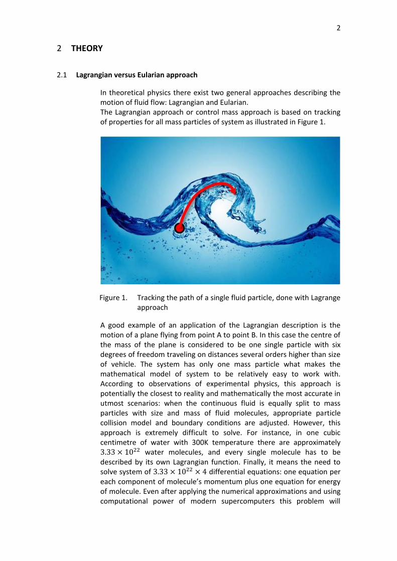
In theoretical physics there exist two general approaches describing the motion of fluid flow: Lagrangian and Eularian. The Lagrangian approach or control mass approach is based on tracking of properties for all mass particles of system as illustrated in Figure 1.

Figure 1. Tracking the path of a single fluid particle, done with Lagrange approach

A good example of an application of the Lagrangian description is the motion of a plane flying from point A to point B. In this case the centre of the mass of the plane is considered to be one single particle with six degrees of freedom traveling on distances several orders higher than size of vehicle. The system has only one mass particle what makes the mathematical model of system to be relatively easy to work with. According to observations of experimental physics, this approach is potentially the closest to reality and mathematically the most accurate in utmost scenarios: when the continuous fluid is equally split to mass particles with size and mass of fluid molecules, appropriate particle collision model and boundary conditions are adjusted. However, this approach is extremely difficult to solve. For instance, in one cubic centimetre of water with 300K temperature there are approximately 3.33 × 1022 water molecules, and every single molecule has to be described by its own Lagrangian function. Finally, it means the need to solve system of 3.33 × 1022 × 4 differential equations: one equation per each component of molecule’s momentum plus one equation for energy of molecule. Even after applying the numerical approximations and using computational power of modern supercomputers this problem will

3

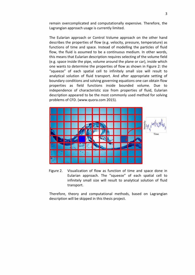
remain overcomplicated and computationally expensive. Therefore, the Lagrangian approach usage is currently limited. The Eularian approach or Control Volume approach on the other hand describes the properties of flow (e.g. velocity, pressure, temperature) as functions of time and space. Instead of modelling the particles of fluid flow, the fluid is assumed to be a continuous medium. In other words, this means that Eularian description requires selecting of the volume field (e.g. space inside the pipe, volume around the plane or car), inside which one wants to determine the properties of flow as shown in Figure 2: the “squeeze” of each spatial cell to infinitely small size will result to analytical solution of fluid transport. And after appropriate setting of boundary conditions and solving governing equations one can obtain flow properties as field functions inside bounded volume. Due to independence of characteristic size from properties of fluid, Eularian description appeared to be the most commonly used method for solving problems of CFD. (www.quora.com 2015).

Figure 2. Visualization of flow as function of time and space done in Eularian approach. The “squeeze” of each spatial cell to infinitely small size will result to analytical solution of fluid transport.

Therefore, theory and computational methods, based on Lagrangian description will be skipped in this thesis project.

4

2.2 Governing equations.

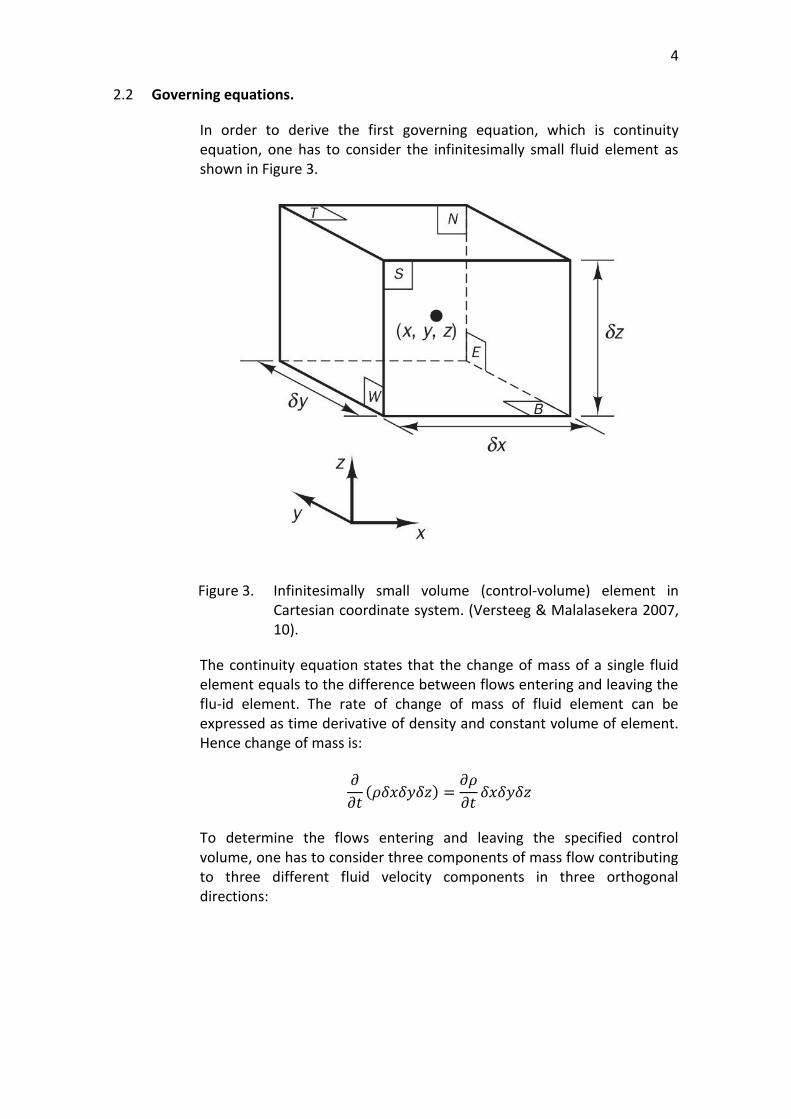
In order to derive the first governing equation, which is continuity equation, one has to consider the infinitesimally small fluid element as shown in Figure 3.

Figure 3. Infinitesimally small volume (control-volume) element in Cartesian coordinate system. (Versteeg & Malalasekera 2007, 10).

The continuity equation states that the change of mass of a single fluid element equals to the difference between flows entering and leaving the flu-id element. The rate of change of mass of fluid element can be expressed as time derivative of density and constant volume of element. Hence change of mass is:

𝜕

𝜕𝑡(𝜌𝛿𝑥𝛿𝑦𝛿𝑧) =

𝜕𝜌

𝜕𝑡𝛿𝑥𝛿𝑦𝛿𝑧

To determine the flows entering and leaving the specified control volume, one has to consider three components of mass flow contributing to three different fluid velocity components in three orthogonal directions:

5

Table 1. Mass flow components due to different fluid velocity components.

Direction Velocity component

Mass flow component in exact centre of volume element

𝑥 𝑢 𝜌𝑢𝛿𝑦𝛿𝑧

𝑦 𝑣 𝜌𝑣𝛿𝑥𝛿𝑧

𝑧 𝑤 𝜌𝑤𝛿𝑥𝛿𝑦

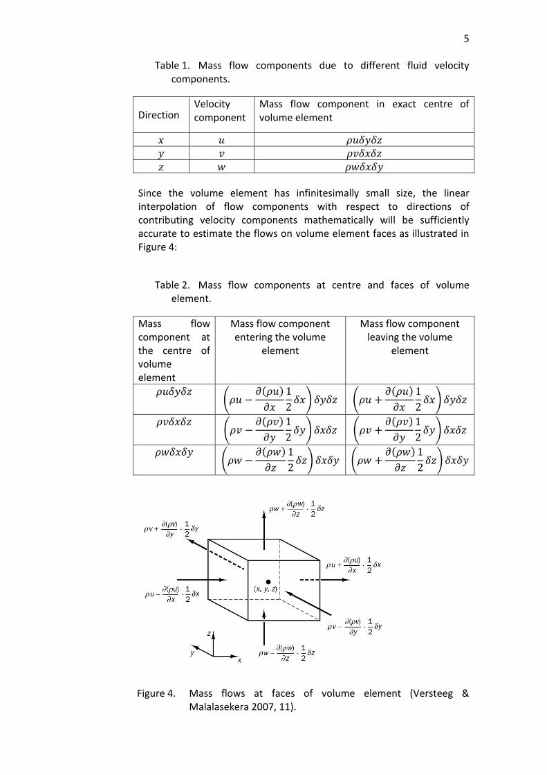
Since the volume element has infinitesimally small size, the linear interpolation of flow components with respect to directions of contributing velocity components mathematically will be sufficiently accurate to estimate the flows on volume element faces as illustrated in Figure 4:

Table 2. Mass flow components at centre and faces of volume element.

Mass flow component at the centre of volume element

Mass flow component entering the volume

element

Mass flow component leaving the volume

element

𝜌𝑢𝛿𝑦𝛿𝑧 (𝜌𝑢 −

𝜕(𝜌𝑢)

𝜕𝑥

1

2𝛿𝑥) 𝛿𝑦𝛿𝑧 (𝜌𝑢 +

𝜕(𝜌𝑢)

𝜕𝑥

1

2𝛿𝑥) 𝛿𝑦𝛿𝑧

𝜌𝑣𝛿𝑥𝛿𝑧 (𝜌𝑣 −

𝜕(𝜌𝑣)

𝜕𝑦

1

2𝛿𝑦) 𝛿𝑥𝛿𝑧 (𝜌𝑣 +

𝜕(𝜌𝑣)

𝜕𝑦

1

2𝛿𝑦) 𝛿𝑥𝛿𝑧

𝜌𝑤𝛿𝑥𝛿𝑦 (𝜌𝑤 −

𝜕(𝜌𝑤)

𝜕𝑧

1

2𝛿𝑧) 𝛿𝑥𝛿𝑦 (𝜌𝑤 +

𝜕(𝜌𝑤)

𝜕𝑧

1

2𝛿𝑧) 𝛿𝑥𝛿𝑦

Figure 4. Mass flows at faces of volume element (Versteeg & Malalasekera 2007, 11).

6

To obtain a flow difference at inlet and outlet faces one has to subtract the summed components at outlet faces from summed components at inlet faces, resulting in:

(𝜌𝑢 −𝜕(𝜌𝑢)

𝜕𝑥

1

2𝛿𝑥) 𝛿𝑦𝛿𝑧 + (𝜌𝑣 −

𝜕(𝜌𝑣)

𝜕𝑦

1

2𝛿𝑦) 𝛿𝑥𝛿𝑧

+ (𝜌𝑤 −𝜕(𝜌𝑤)

𝜕𝑧

1

2𝛿𝑧) 𝛿𝑥𝛿𝑦 − (𝜌𝑢 +

𝜕(𝜌𝑢)

𝜕𝑥

1

2𝛿𝑥) 𝛿𝑦𝛿𝑧

− (𝜌𝑣 +𝜕(𝜌𝑣)

𝜕𝑦

1

2𝛿𝑦) 𝛿𝑥𝛿𝑧 − (𝜌𝑤 +

𝜕(𝜌𝑤)

𝜕𝑧

1

2𝛿𝑧)𝛿𝑥𝛿𝑦

= −(𝜕(𝜌𝑢)

𝜕𝑥+

𝜕(𝜌𝑣)

𝜕𝑦+

𝜕(𝜌𝑤)

𝜕𝑧)𝛿𝑥𝛿𝑦𝛿𝑧

Finally, after the setting of equality sign between the rate of change of mass and mass flow difference will result in:

𝜕𝜌

𝜕𝑡𝛿𝑥𝛿𝑦𝛿𝑧 = −(

𝜕(𝜌𝑢)

𝜕𝑥+

𝜕(𝜌𝑣)

𝜕𝑦+

𝜕(𝜌𝑤)

𝜕𝑧)𝛿𝑥𝛿𝑦𝛿𝑧

That after several trivial rearrangements can be simplified to final form of mass continuity equation (Versteeg & Malalasekera 2007, 9 - 11):

0 =𝜕𝜌

𝜕𝑡+ 𝑑𝑖𝑣(𝜌𝐮)

(2.2.1) Where:

𝑑𝑖𝑣(ρ𝐮) ≡𝜕(𝜌𝑢)

𝜕𝑥+

𝜕(𝜌𝑣)

𝜕𝑦+

𝜕(𝜌𝑤)

𝜕𝑧

(2.2.2) 𝜌 – Is fluid density as a field function of (𝑥; 𝑦; 𝑧; 𝑡). 𝑢 – Is component of velocity vector u towards x-direction as a field function of (𝑥; 𝑦; 𝑧; 𝑡). 𝑣 – Is component of velocity vector u towards y-direction as a field function of (𝑥; 𝑦; 𝑧; 𝑡). 𝑤 – Is component of velocity vector u towards z-direction as a field function of (𝑥; 𝑦; 𝑧; 𝑡). 𝑡 – Is time. Or:

𝐮 = [𝑢𝑣𝑤

]

(𝑥)(𝑦)(𝑧)

(2.2.3)

7

“𝑑𝑖𝑣(𝐚)” is called a divergence of vector “𝐚” (alternative notation: ∇ ∙ 𝐚). As an example, for vector a in Cartesian coordinate system:

𝐚 = [

𝑎𝑥

𝑎𝑦

𝑎𝑧

]

𝑑𝑖𝑣(𝐚) ≡ ∇ ∙ 𝐚 =𝜕𝑎𝑥

𝜕𝑥+

𝜕𝑎𝑦

𝜕𝑦+

𝜕𝑎𝑧

𝜕𝑧

Equation 2.2.1 is valid for unsteady compressible three-dimensional flow. Further assumption of incompressible, steady flow will lead to next form of continuity differential equation:

0 =𝜕𝑢

𝜕𝑥+

𝜕𝑣

𝜕𝑦+

𝜕𝑤

𝜕𝑧

(2.2.4) for three-dimensional incompressible flow, and:

0 =𝜕𝑢

𝜕𝑥+

𝜕𝑣

𝜕𝑦

(2.2.5) for two-dimensional incompressible flow. One can also show that term, equal to zero in eq. 2.2.1 is just one possible form of more generalized term:

𝜕(𝜌𝜑)

𝜕𝑡+ 𝑑𝑖𝑣(𝜌𝜑𝐮)

(2.2.6) Where: φ – is arbitrary conservative intensive property (e.g. mass, momentum, or energy per unit mass). (Versteeg & Malalasekera 2007, 12 - 14). That combined with eq.2.2.1 can be further simplified to:

𝜕(𝜌𝜑)

𝜕𝑡+ 𝑑𝑖𝑣(𝜌𝜑𝐮) = 𝜌

𝐷𝜑

𝐷𝑡

(2.2.7) Where: 𝐷

𝐷𝑡 – is material derivative operator. Other names of material derivative

are advective, convective, hydrodynamic, Lagrangian, particle, substantial, substantive, Stokes or total derivative.

8

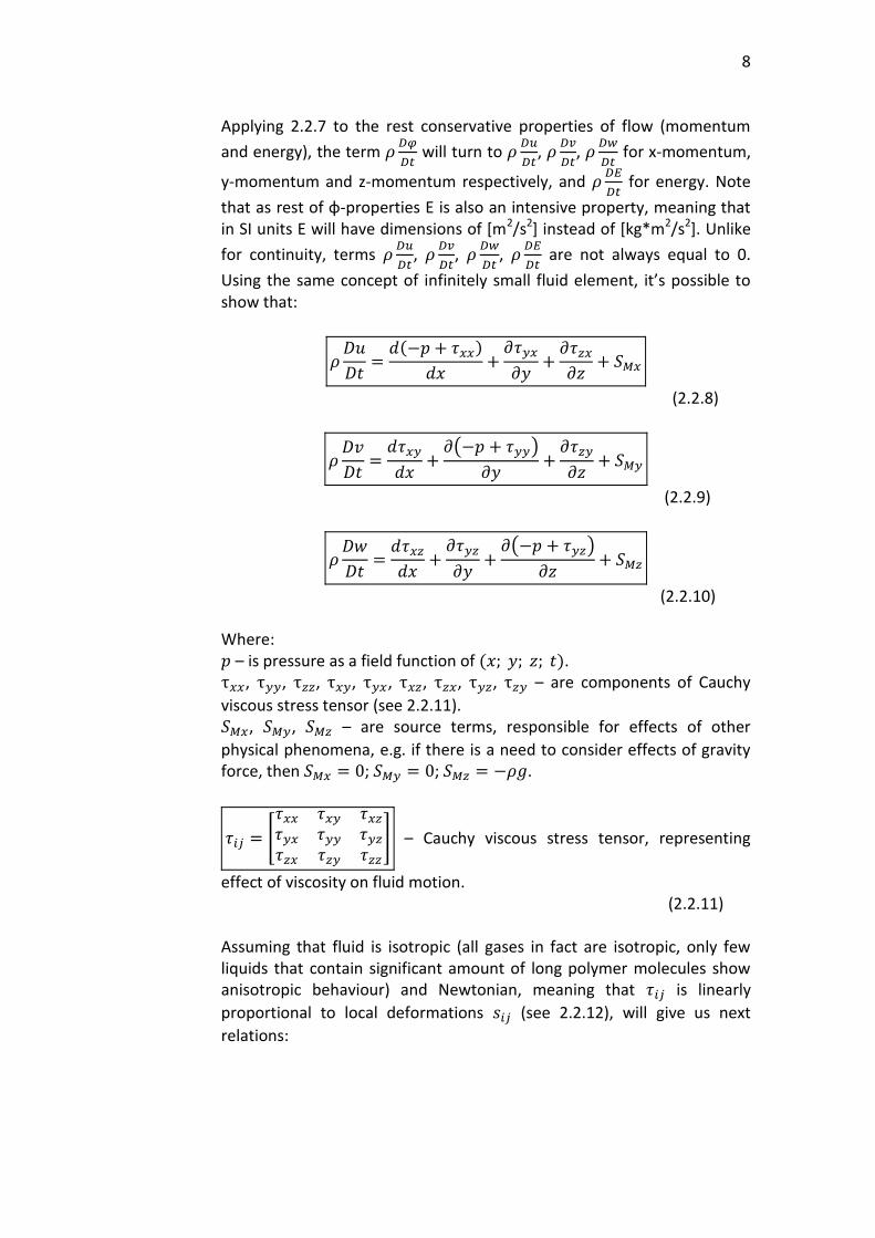
Applying 2.2.7 to the rest conservative properties of flow (momentum

and energy), the term 𝜌𝐷𝜑

𝐷𝑡 will turn to 𝜌

𝐷𝑢

𝐷𝑡, 𝜌

𝐷𝑣

𝐷𝑡, 𝜌

𝐷𝑤

𝐷𝑡 for x-momentum,

y-momentum and z-momentum respectively, and 𝜌𝐷𝐸

𝐷𝑡 for energy. Note

that as rest of φ-properties E is also an intensive property, meaning that in SI units E will have dimensions of [m2/s2] instead of [kg*m2/s2]. Unlike

for continuity, terms 𝜌𝐷𝑢

𝐷𝑡, 𝜌

𝐷𝑣

𝐷𝑡, 𝜌

𝐷𝑤

𝐷𝑡, 𝜌

𝐷𝐸

𝐷𝑡 are not always equal to 0.

Using the same concept of infinitely small fluid element, it’s possible to show that:

𝜌𝐷𝑢

𝐷𝑡=

𝑑(−𝑝 + 𝜏𝑥𝑥)

𝑑𝑥+

𝜕𝜏𝑦𝑥

𝜕𝑦+

𝜕𝜏𝑧𝑥

𝜕𝑧+ 𝑆𝑀𝑥

(2.2.8)

𝜌𝐷𝑣

𝐷𝑡=

𝑑𝜏𝑥𝑦

𝑑𝑥+

𝜕(−𝑝 + 𝜏𝑦𝑦)

𝜕𝑦+

𝜕𝜏𝑧𝑦

𝜕𝑧+ 𝑆𝑀𝑦

(2.2.9)

𝜌𝐷𝑤

𝐷𝑡=

𝑑𝜏𝑥𝑧

𝑑𝑥+

𝜕𝜏𝑦𝑧

𝜕𝑦+

𝜕(−𝑝 + 𝜏𝑦𝑧)

𝜕𝑧+ 𝑆𝑀𝑧

(2.2.10) Where: 𝑝 – is pressure as a field function of (𝑥; 𝑦; 𝑧; 𝑡). τ𝑥𝑥, τ𝑦𝑦, τ𝑧𝑧, τ𝑥𝑦, τ𝑦𝑥, τ𝑥𝑧, τ𝑧𝑥, τ𝑦𝑧, τ𝑧𝑦 – are components of Cauchy

viscous stress tensor (see 2.2.11). 𝑆𝑀𝑥, 𝑆𝑀𝑦, 𝑆𝑀𝑧 – are source terms, responsible for effects of other

physical phenomena, e.g. if there is a need to consider effects of gravity force, then 𝑆𝑀𝑥 = 0; 𝑆𝑀𝑦 = 0; 𝑆𝑀𝑧 = −𝜌𝑔.

𝜏𝑖𝑗 = [

𝜏𝑥𝑥 𝜏𝑥𝑦 𝜏𝑥𝑧

𝜏𝑦𝑥 𝜏𝑦𝑦 𝜏𝑦𝑧

𝜏𝑧𝑥 𝜏𝑧𝑦 𝜏𝑧𝑧

] – Cauchy viscous stress tensor, representing

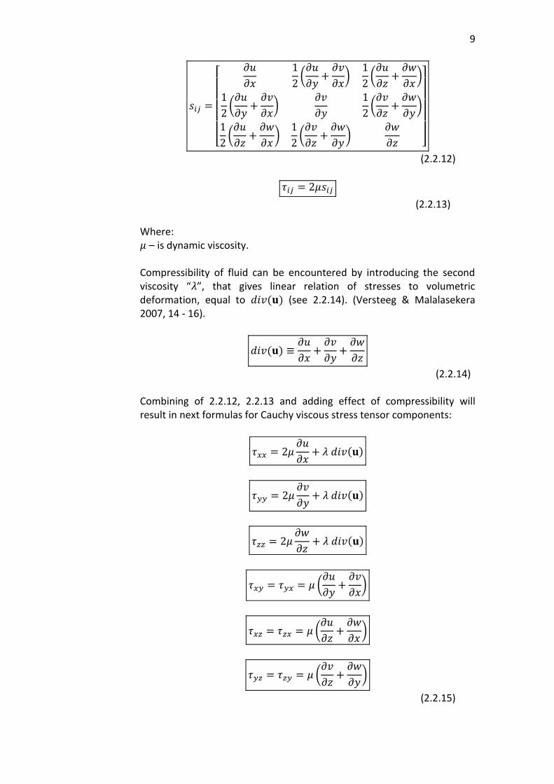
effect of viscosity on fluid motion. (2.2.11) Assuming that fluid is isotropic (all gases in fact are isotropic, only few liquids that contain significant amount of long polymer molecules show anisotropic behaviour) and Newtonian, meaning that 𝜏𝑖𝑗 is linearly

proportional to local deformations 𝑠𝑖𝑗 (see 2.2.12), will give us next

relations:

9

𝑠𝑖𝑗 =

[

𝜕𝑢

𝜕𝑥

1

2(𝜕𝑢

𝜕𝑦+

𝜕𝑣

𝜕𝑥)

1

2(𝜕𝑢

𝜕𝑧+

𝜕𝑤

𝜕𝑥)

1

2(𝜕𝑢

𝜕𝑦+

𝜕𝑣

𝜕𝑥)

𝜕𝑣

𝜕𝑦

1

2(𝜕𝑣

𝜕𝑧+

𝜕𝑤

𝜕𝑦)

1

2(𝜕𝑢

𝜕𝑧+

𝜕𝑤

𝜕𝑥)

1

2(𝜕𝑣

𝜕𝑧+

𝜕𝑤

𝜕𝑦)

𝜕𝑤

𝜕𝑧 ]

(2.2.12)

𝜏𝑖𝑗 = 2𝜇𝑠𝑖𝑗

(2.2.13) Where: 𝜇 – is dynamic viscosity. Compressibility of fluid can be encountered by introducing the second viscosity “𝜆”, that gives linear relation of stresses to volumetric deformation, equal to 𝑑𝑖𝑣(𝐮) (see 2.2.14). (Versteeg & Malalasekera 2007, 14 - 16).

𝑑𝑖𝑣(𝐮) ≡𝜕𝑢

𝜕𝑥+

𝜕𝑣

𝜕𝑦+

𝜕𝑤

𝜕𝑧

(2.2.14) Combining of 2.2.12, 2.2.13 and adding effect of compressibility will result in next formulas for Cauchy viscous stress tensor components:

𝜏𝑥𝑥 = 2𝜇𝜕𝑢

𝜕𝑥+ 𝜆 𝑑𝑖𝑣(𝐮)

𝜏𝑦𝑦 = 2𝜇𝜕𝑣

𝜕𝑦+ 𝜆 𝑑𝑖𝑣(𝐮)

𝜏𝑧𝑧 = 2𝜇𝜕𝑤

𝜕𝑧+ 𝜆 𝑑𝑖𝑣(𝐮)

𝜏𝑥𝑦 = 𝜏𝑦𝑥 = 𝜇 (𝜕𝑢

𝜕𝑦+

𝜕𝑣

𝜕𝑥)

𝜏𝑥𝑧 = 𝜏𝑧𝑥 = 𝜇 (𝜕𝑢

𝜕𝑧+

𝜕𝑤

𝜕𝑥)

𝜏𝑦𝑧 = 𝜏𝑧𝑦 = 𝜇 (𝜕𝑣

𝜕𝑧+

𝜕𝑤

𝜕𝑦)

(2.2.15)

10

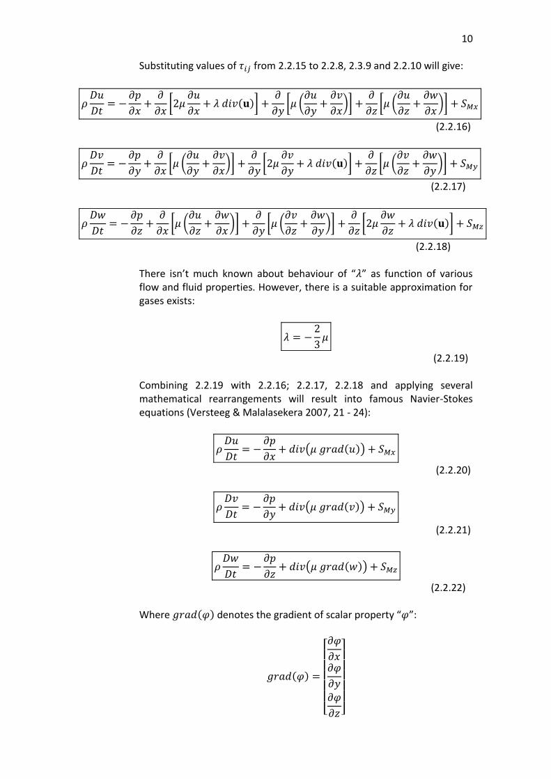
Substituting values of 𝜏𝑖𝑗 from 2.2.15 to 2.2.8, 2.3.9 and 2.2.10 will give:

𝜌𝐷𝑢

𝐷𝑡= −

𝜕𝑝

𝜕𝑥+

𝜕

𝜕𝑥[2𝜇

𝜕𝑢

𝜕𝑥+ 𝜆 𝑑𝑖𝑣(𝐮)] +

𝜕

𝜕𝑦[𝜇 (

𝜕𝑢

𝜕𝑦+

𝜕𝑣

𝜕𝑥)] +

𝜕

𝜕𝑧[𝜇 (

𝜕𝑢

𝜕𝑧+

𝜕𝑤

𝜕𝑥)] + 𝑆𝑀𝑥

(2.2.16)

𝜌𝐷𝑣

𝐷𝑡= −

𝜕𝑝

𝜕𝑦+

𝜕

𝜕𝑥[𝜇 (

𝜕𝑢

𝜕𝑦+

𝜕𝑣

𝜕𝑥)] +

𝜕

𝜕𝑦[2𝜇

𝜕𝑣

𝜕𝑦+ 𝜆 𝑑𝑖𝑣(𝐮)] +

𝜕

𝜕𝑧[𝜇 (

𝜕𝑣

𝜕𝑧+

𝜕𝑤

𝜕𝑦)] + 𝑆𝑀𝑦

(2.2.17)

𝜌𝐷𝑤

𝐷𝑡= −

𝜕𝑝

𝜕𝑧+

𝜕

𝜕𝑥[𝜇 (

𝜕𝑢

𝜕𝑧+

𝜕𝑤

𝜕𝑥)] +

𝜕

𝜕𝑦[𝜇 (

𝜕𝑣

𝜕𝑧+

𝜕𝑤

𝜕𝑦)] +

𝜕

𝜕𝑧[2𝜇

𝜕𝑤

𝜕𝑧+ 𝜆 𝑑𝑖𝑣(𝐮)] + 𝑆𝑀𝑧

(2.2.18) There isn’t much known about behaviour of “𝜆” as function of various flow and fluid properties. However, there is a suitable approximation for gases exists:

𝜆 = −2

3𝜇

(2.2.19) Combining 2.2.19 with 2.2.16; 2.2.17, 2.2.18 and applying several mathematical rearrangements will result into famous Navier-Stokes equations (Versteeg & Malalasekera 2007, 21 - 24):

𝜌𝐷𝑢

𝐷𝑡= −

𝜕𝑝

𝜕𝑥+ 𝑑𝑖𝑣(𝜇 𝑔𝑟𝑎𝑑(𝑢)) + 𝑆𝑀𝑥

(2.2.20)

𝜌𝐷𝑣

𝐷𝑡= −

𝜕𝑝

𝜕𝑦+ 𝑑𝑖𝑣(𝜇 𝑔𝑟𝑎𝑑(𝑣)) + 𝑆𝑀𝑦

(2.2.21)

𝜌𝐷𝑤

𝐷𝑡= −

𝜕𝑝

𝜕𝑧+ 𝑑𝑖𝑣(𝜇 𝑔𝑟𝑎𝑑(𝑤)) + 𝑆𝑀𝑧

(2.2.22) Where 𝑔𝑟𝑎𝑑(𝜑) denotes the gradient of scalar property “𝜑”:

𝑔𝑟𝑎𝑑(𝜑) =

[ 𝜕𝜑

𝜕𝑥𝜕𝜑

𝜕𝑦𝜕𝜑

𝜕𝑧]

11

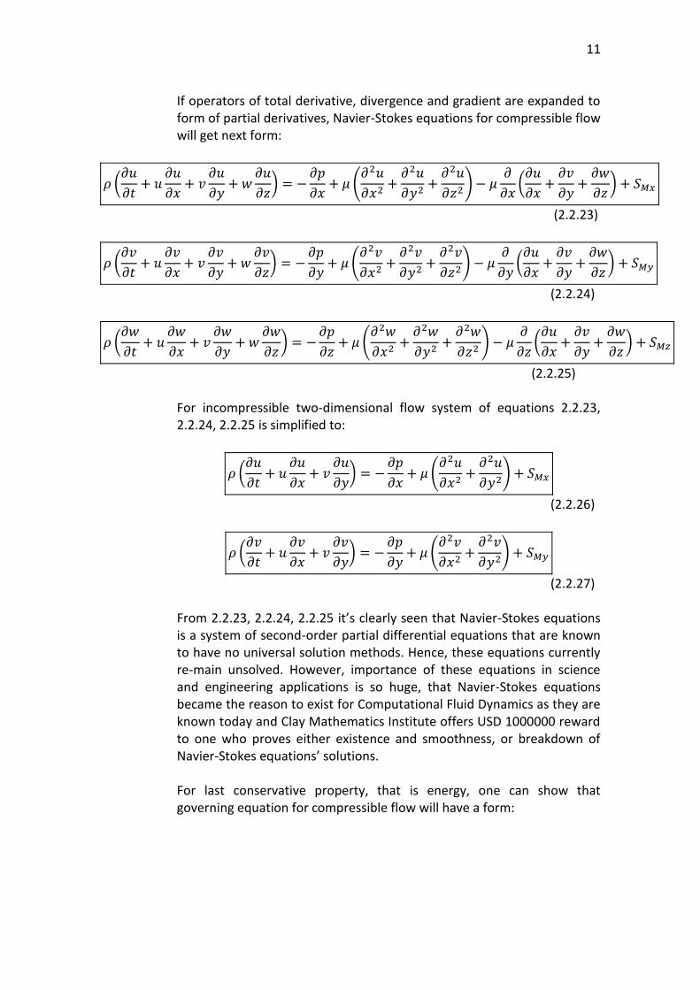
If operators of total derivative, divergence and gradient are expanded to form of partial derivatives, Navier-Stokes equations for compressible flow will get next form:

𝜌 (𝜕𝑢

𝜕𝑡+ 𝑢

𝜕𝑢

𝜕𝑥+ 𝑣

𝜕𝑢

𝜕𝑦+ 𝑤

𝜕𝑢

𝜕𝑧) = −

𝜕𝑝

𝜕𝑥+ 𝜇 (

𝜕2𝑢

𝜕𝑥2+

𝜕2𝑢

𝜕𝑦2+

𝜕2𝑢

𝜕𝑧2) − 𝜇

𝜕

𝜕𝑥(𝜕𝑢

𝜕𝑥+

𝜕𝑣

𝜕𝑦+

𝜕𝑤

𝜕𝑧) + 𝑆𝑀𝑥

(2.2.23)

𝜌 (𝜕𝑣

𝜕𝑡+ 𝑢

𝜕𝑣

𝜕𝑥+ 𝑣

𝜕𝑣

𝜕𝑦+ 𝑤

𝜕𝑣

𝜕𝑧) = −

𝜕𝑝

𝜕𝑦+ 𝜇 (

𝜕2𝑣

𝜕𝑥2+

𝜕2𝑣

𝜕𝑦2+

𝜕2𝑣

𝜕𝑧2) − 𝜇

𝜕

𝜕𝑦(𝜕𝑢

𝜕𝑥+

𝜕𝑣

𝜕𝑦+

𝜕𝑤

𝜕𝑧) + 𝑆𝑀𝑦

(2.2.24)

𝜌 (𝜕𝑤

𝜕𝑡+ 𝑢

𝜕𝑤

𝜕𝑥+ 𝑣

𝜕𝑤

𝜕𝑦+ 𝑤

𝜕𝑤

𝜕𝑧) = −

𝜕𝑝

𝜕𝑧+ 𝜇 (

𝜕2𝑤

𝜕𝑥2+

𝜕2𝑤

𝜕𝑦2+

𝜕2𝑤

𝜕𝑧2) − 𝜇

𝜕

𝜕𝑧(𝜕𝑢

𝜕𝑥+

𝜕𝑣

𝜕𝑦+

𝜕𝑤

𝜕𝑧) + 𝑆𝑀𝑧

(2.2.25) For incompressible two-dimensional flow system of equations 2.2.23, 2.2.24, 2.2.25 is simplified to:

𝜌 (𝜕𝑢

𝜕𝑡+ 𝑢

𝜕𝑢

𝜕𝑥+ 𝑣

𝜕𝑢

𝜕𝑦) = −

𝜕𝑝

𝜕𝑥+ 𝜇 (

𝜕2𝑢

𝜕𝑥2+

𝜕2𝑢

𝜕𝑦2) + 𝑆𝑀𝑥

(2.2.26)

𝜌 (𝜕𝑣

𝜕𝑡+ 𝑢

𝜕𝑣

𝜕𝑥+ 𝑣

𝜕𝑣

𝜕𝑦) = −

𝜕𝑝

𝜕𝑦+ 𝜇 (

𝜕2𝑣

𝜕𝑥2+

𝜕2𝑣

𝜕𝑦2) + 𝑆𝑀𝑦

(2.2.27) From 2.2.23, 2.2.24, 2.2.25 it’s clearly seen that Navier-Stokes equations is a system of second-order partial differential equations that are known to have no universal solution methods. Hence, these equations currently re-main unsolved. However, importance of these equations in science and engineering applications is so huge, that Navier-Stokes equations became the reason to exist for Computational Fluid Dynamics as they are known today and Clay Mathematics Institute offers USD 1000000 reward to one who proves either existence and smoothness, or breakdown of Navier-Stokes equations’ solutions. For last conservative property, that is energy, one can show that governing equation for compressible flow will have a form:

12

𝜌𝐷𝐸

𝐷𝑡= −𝑑𝑖𝑣(𝑝𝐮) + 𝑑𝑖𝑣(𝑘 𝑔𝑟𝑎𝑑(𝑇))

+ [𝜕(𝑢𝜏𝑥𝑥)

𝜕𝑥+

𝜕(𝑣𝜏𝑦𝑥)

𝜕𝑦+

𝜕(𝑤𝜏𝑧𝑥)

𝜕𝑧+

𝜕(𝑢𝜏𝑥𝑦)

𝜕𝑥+

𝜕(𝑣𝜏𝑦𝑦)

𝜕𝑦+

𝜕(𝑤𝜏𝑧𝑦)

𝜕𝑧

+𝜕(𝑢𝜏𝑥𝑧)

𝜕𝑥+

𝜕(𝑣𝜏𝑦𝑧)

𝜕𝑦+

𝜕(𝑤𝜏𝑧𝑧)

𝜕𝑧] + 𝑆𝐸

(2.2.28) Where:

𝐸 = 𝑖 +1

2(𝑢2 + 𝑣2 + 𝑤2) – sum of kinetic and internal energy.

𝑖 = 𝐶𝑉𝑇

𝑘 – is thermal conductivity of fluid. 𝑇 – is temperature. 𝐶𝑉– is molar heat capacity of gas under constant volume. Sometimes it might be useful to rearrange 2.2.28, using such properties as internal energy (2.2.29), temperature (2.2.30) or total enthalpy (2.2.31):

𝜌𝐷𝑖

𝐷𝑡= −𝑝 𝑑𝑖𝑣(𝐮) + 𝑑𝑖𝑣(𝑘 𝑔𝑟𝑎𝑑(𝑇))


𝜕𝑥+


𝜕𝑦+


𝜕𝑧+


𝜕𝑥+


𝜕𝑦+


𝜕𝑧


𝜕𝑥+


𝜕𝑦+


𝜕𝑧] + 𝑆𝑖

(2.2.29)

𝜌𝐶𝑉

𝐷𝑇

𝐷𝑡= −𝑝 𝑑𝑖𝑣(𝐮) + 𝑑𝑖𝑣(𝑘 𝑔𝑟𝑎𝑑(𝑇))


𝜕𝑥+


𝜕𝑦+


𝜕𝑧+


𝜕𝑥+


𝜕𝑦+


𝜕𝑧


𝜕𝑥+


𝜕𝑦+


𝜕𝑧] + 𝑆𝑖

(2.2.30)

𝜌𝐷ℎ0

𝐷𝑡=

𝜕𝑝

𝜕𝑡+ 𝑑𝑖𝑣(𝑘 𝑔𝑟𝑎𝑑(𝑇))


𝜕𝑥+


𝜕𝑦+


𝜕𝑧+


𝜕𝑥+


𝜕𝑦+


𝜕𝑧


𝜕𝑥+


𝜕𝑦+


𝜕𝑧] + 𝑆ℎ

(2.2.31) Where:

ℎ = 𝑖 +𝑝

𝜌 – is enthalpy of gas.

13

ℎ0 = ℎ +1

2(𝑢2 + 𝑣2 + 𝑤2) – is total enthalpy.

Application of Newtonian viscosity model to eq.2.2.29 will yield to:

𝜌𝐶𝑉

𝐷𝑇

𝐷𝑡= −𝑝 𝑑𝑖𝑣(𝐮) + 𝑑𝑖𝑣(𝑘 𝑔𝑟𝑎𝑑(𝑇)) + 𝛷 + 𝑆𝑖

(2.2.32) Where:

𝛷 = 𝜇 {2 [(𝜕𝑢

𝜕𝑥)2

+ (𝜕𝑣

𝜕𝑦)2

+ (𝜕𝑤

𝜕𝑧)2

] + (𝜕𝑢

𝜕𝑦+

𝜕𝑣

𝜕𝑥)

2

+ (𝜕𝑢

𝜕𝑧+

𝜕𝑤

𝜕𝑥)2

+ (𝜕𝑣

𝜕𝑧+

𝜕𝑤

𝜕𝑦)2

} + 𝜆(𝑑𝑖𝑣(𝐮))2

(2.2.33) Together equations 2.2.1, 2.2.20, 2.2.21, 2.2.22, 2.2.29 and such equations of state as ideal gas equation (𝑝𝑉 = 𝑛𝑅𝑇) and internal energy equation (𝑖 = 𝐶𝑉𝑇) are forming the system of seven equations with seven unknowns, meaning that system is mathematically closed (it can be solved, providing that initial and boundary conditions are stated). (Versteeg & Malalasekera 2007, 18 - 21). 2.2.1, 2.2.20, 2.2.21, 2.2.22, 2.2.29 can be generalized, using arbitrary property 𝜑:

𝜕(𝜌𝜑)

𝜕𝑡+ div(𝜌𝜑𝐮) = 𝑑𝑖𝑣(𝛤 𝑔𝑟𝑎𝑑(𝜑)) + 𝑆𝜑

(2.2.34) Where 𝛤 – is diffusion coefficient such as viscosity 𝜇, or conductivity 𝑘. The eq.2.2.34 is called transport equation of property 𝜑, which can be changed back to equations 2.2.1, 2.2.20, 2.2.21, 2.2.22, 2.2.29 by setting the property 𝜑 to be equal to 1, 𝑢, 𝑣, 𝑤 or 𝑖 respectively and appropriately setting of source terms and values of 𝛤. In order to get form of eq.2.2.34, more convenient for finite volume method, the integration over Control volume must be applied to eq.2.2.34:

∫𝜕(𝜌𝜑)

𝜕𝑡𝑑𝑉

𝐶𝑉

+ ∫𝑑𝑖𝑣(𝜌𝜑𝐮)𝑑𝑉

𝐶𝑉

= ∫𝑑𝑖𝑣(𝛤 𝑔𝑟𝑎𝑑(𝜑))𝑑𝑉

𝐶𝑉

+ ∫𝑆𝜑𝑑𝑉

𝐶𝑉

(2.2.35) Where: 𝑉 – is volume. CV – is reference to control volume. CS – is reference to control surface (boundary of control volume).

14

For further transforming of 2.2.35, there is a need to introduce Gauss’s divergence theorem, stating, that for vector “𝐚”:

∫𝑑𝑖𝑣(𝐚)𝑑𝑉 = ∫𝐧. 𝐚𝑑𝐴

CS

CV

(2.2.36) Where: 𝐴 – is area. 𝐧. 𝐚 – is component of vector “𝐚” in the direction of unit vector “𝐧”, normal to surface element 𝑑𝐴. Applying Gauss’s divergence theorem (2.2.36) and changing the order of integration and differentiation in first term in left-hand side of eq.2.2.35 will yield to:

𝜕

𝜕𝑡( ∫(𝜌𝜑)𝑑𝑉

𝐶𝑉

) + ∫𝐧. (𝜌𝜑𝐮)𝑑𝐴

𝐶𝑆

= ∫ 𝐧. (𝛤 𝑔𝑟𝑎𝑑(𝜑))𝑑𝐴

𝐶𝑆


𝐶𝑉

(2.2.37) To derive the most general integrated form of transport equation, the integration over time interval from t to 𝑡 + 𝛥𝑡 must be applied in order to cover time-dependant problems. (Versteeg & Malalasekera 2007, 24 - 26):

∫𝜕

𝜕𝑡( ∫(𝜌𝜑)𝑑𝑉

𝐶𝑉

)𝑑𝑡

𝛥𝑡

+ ∫ ∫𝐧. (𝜌𝜑𝐮)𝑑𝐴𝑑𝑡

𝐶𝑆

𝛥𝑡

= ∫ ∫𝐧. (𝛤 𝑔𝑟𝑎𝑑(𝜑))𝑑𝐴𝑑𝑡

𝐶𝑆

𝛥𝑡

+ ∫ ∫𝑆𝜑𝑑𝑉𝑑𝑡

𝐶𝑉

𝛥𝑡

(2.2.38)

15

2.3 Turbulence

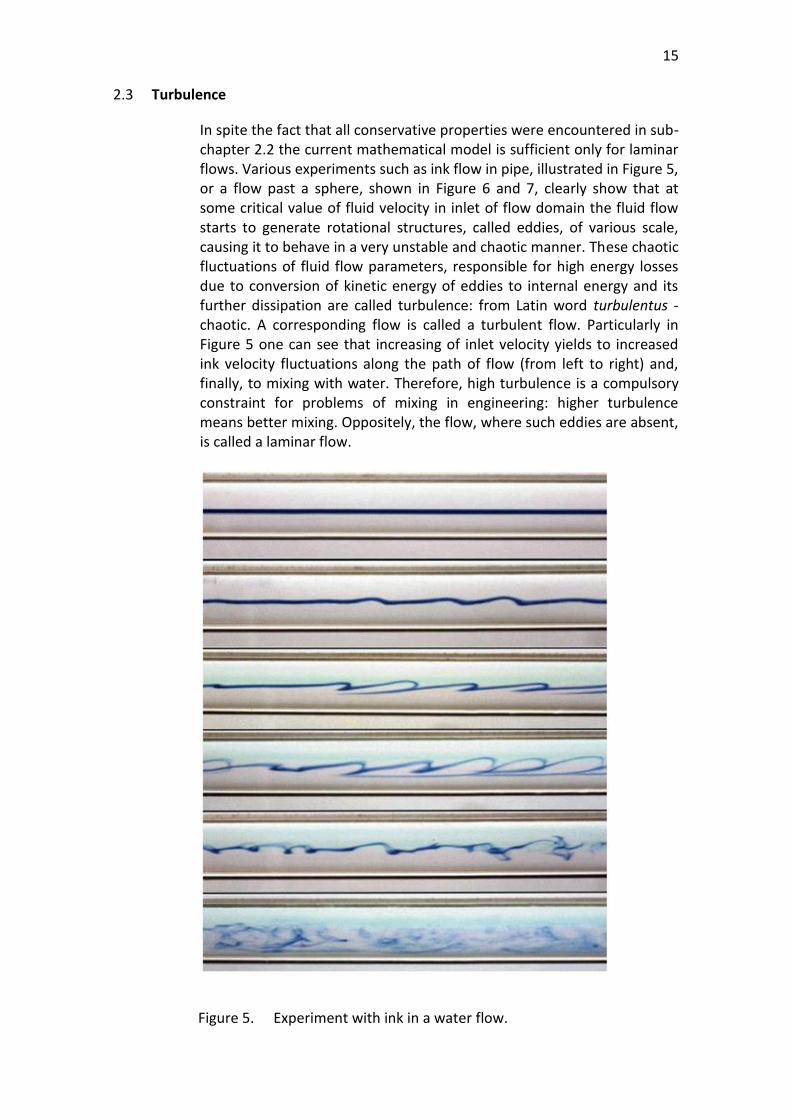
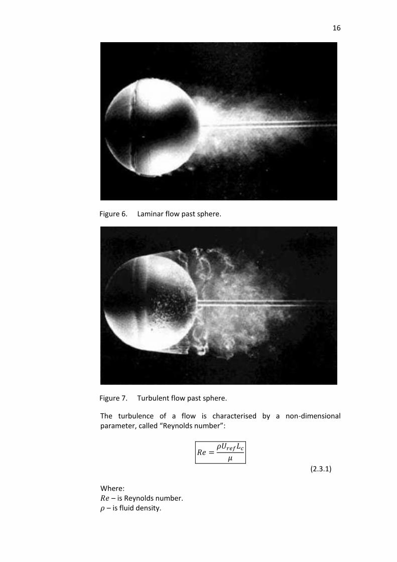
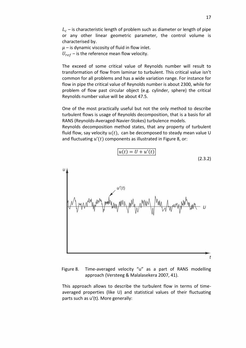
In spite the fact that all conservative properties were encountered in sub-chapter 2.2 the current mathematical model is sufficient only for laminar flows. Various experiments such as ink flow in pipe, illustrated in Figure 5, or a flow past a sphere, shown in Figure 6 and 7, clearly show that at some critical value of fluid velocity in inlet of flow domain the fluid flow starts to generate rotational structures, called eddies, of various scale, causing it to behave in a very unstable and chaotic manner. These chaotic fluctuations of fluid flow parameters, responsible for high energy losses due to conversion of kinetic energy of eddies to internal energy and its further dissipation are called turbulence: from Latin word turbulentus - chaotic. A corresponding flow is called a turbulent flow. Particularly in Figure 5 one can see that increasing of inlet velocity yields to increased ink velocity fluctuations along the path of flow (from left to right) and, finally, to mixing with water. Therefore, high turbulence is a compulsory constraint for problems of mixing in engineering: higher turbulence means better mixing. Oppositely, the flow, where such eddies are absent, is called a laminar flow.

Figure 5. Experiment with ink in a water flow.

16

Figure 6. Laminar flow past sphere.

Figure 7. Turbulent flow past sphere.

The turbulence of a flow is characterised by a non-dimensional parameter, called “Reynolds number”:

𝑅𝑒 =𝜌𝑈𝑟𝑒𝑓𝐿𝑐

𝜇

(2.3.1) Where: 𝑅𝑒 – is Reynolds number. 𝜌 – is fluid density.

17

𝐿𝑐 – is characteristic length of problem such as diameter or length of pipe or any other linear geometric parameter, the control volume is characterised by. 𝜇 – is dynamic viscosity of fluid in flow inlet. 𝑈𝑟𝑒𝑓 – is the reference mean flow velocity.

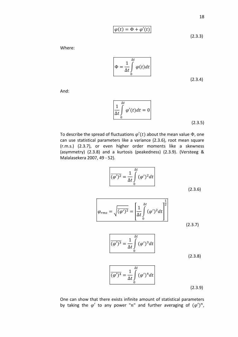
The exceed of some critical value of Reynolds number will result to transformation of flow from laminar to turbulent. This critical value isn’t common for all problems and has a wide variation range. For instance for flow in pipe the critical value of Reynolds number is about 2300, while for problem of flow past circular object (e.g. cylinder, sphere) the critical Reynolds number value will be about 47.5. One of the most practically useful but not the only method to describe turbulent flows is usage of Reynolds decomposition, that is a basis for all RANS (Reynolds-Averaged-Navier-Stokes) turbulence models. Reynolds decomposition method states, that any property of turbulent fluid flow, say velocity 𝑢(𝑡), can be decomposed to steady mean value U and fluctuating 𝑢’(𝑡) components as illustrated in Figure 8, or:

𝑢(𝑡) = 𝑈 + 𝑢′(𝑡)

(2.3.2)

Figure 8. Time-averaged velocity “u” as a part of RANS modelling approach (Versteeg & Malalasekera 2007, 41).

This approach allows to describe the turbulent flow in terms of time-averaged properties (like U) and statistical values of their fluctuating parts such as u’(t). More generally:

18

𝜑(𝑡) = Φ + 𝜑′(𝑡)

(2.3.3) Where:

Φ =1

∆𝑡∫ 𝜑(𝑡)𝑑𝑡

∆𝑡

0

(2.3.4) And:

1

∆𝑡∫ 𝜑′(𝑡)𝑑𝑡

∆𝑡

0

= 0

(2.3.5) To describe the spread of fluctuations 𝜑′(𝑡) about the mean value Φ, one can use statistical parameters like a variance (2.3.6), root mean square (r.m.s.) (2.3.7), or even higher order moments like a skewness (asymmetry) (2.3.8) and a kurtosis (peakedness) (2.3.9). (Versteeg & Malalasekera 2007, 49 - 52).

(𝜑′)2 =1

∆𝑡∫(𝜑′)2𝑑𝑡

∆𝑡

0

(2.3.6)

𝜑𝑟𝑚𝑠 = √(𝜑′)2 = [1

∆𝑡∫ (𝜑′)2𝑑𝑡

∆𝑡

0

]

12

(2.3.7)

(𝜑′)3 =1


∆𝑡

0

(2.3.8)

(𝜑′)4 =1


∆𝑡

0

(2.3.9) One can show that there exists infinite amount of statistical parameters by taking the 𝜑′ to any power "𝑛" and further averaging of (𝜑′)𝑛,

19

however, except variance and root mean square, all these parameters are rarely used in today turbulence modelling problems. On the other hand, variance has a straight connection to total kinetic energy of turbulence "𝑘" per unit mass at certain point:

𝑘 =1

2[ (𝑢′)2 + (𝑣′)2 + (𝑤′)2 ]

(2.3.10) The turbulence intensity 𝑇𝑖, which is another important parameter for RANS turbulence models often used for boundary condition specification in CFD codes, is also related with velocity variance by linkage with "𝑘":

𝑇𝑖 =(23𝑘)

12

𝑈𝑟𝑒𝑓

(2.3.11)

Where term (2

3𝑘)

1

2 is indeed an average r.m.s. velocity of fluid.

The variance is also called the second moment of the fluctuations (similarly third and fourth moments of fluctuations for skewness and kurtosis respectively). Important information about a fluid flow is also contained in moments, constructed from two different variables. As an example one can consider two arbitrary properties 𝜑 and 𝜓. Applying 2.3.3, one defines the second moment of 𝜑′ and 𝜓′ as follows:

𝜑′𝜓′ =1

∆𝑡∫ 𝜑′𝜓′𝑑𝑡

∆𝑡

0

(2.3.12) Such second moments are especially crucial in RANS turbulence due to their usage in description of an additional shear stress experienced by fluid in turbulent flow. Another application of second moments are autocorrelation functions, used to study relations between fluctuations at different time instants and space points. Autocorrelation functions are defined as follows:

𝑅𝜑′𝜑′(𝜏) = 𝜑′(𝑡)𝜑(𝑡 + 𝜏) =1

∆𝑡∫ 𝜑′(𝑡)𝜑′(𝑡 + 𝜏)𝑑𝑡

∆𝑡

0

(2.3.13) (autocorrelation function for different time instants)

20

𝑅𝜑′𝜑′(𝜉) = 𝜑′(𝒙; 𝑡)𝜑′(𝐱 + 𝜉; 𝑡) =1

∆𝑡∫ 𝜑′(𝐱; 𝑡′)𝜑′(𝐱 + 𝜉; 𝑡′

𝑡+∆𝑡

𝑡

)𝑑𝑡′

(2.3.14) (autocorrelation function for two points displaced by vector ±ξ from each other) Where: 𝜏 is a time shift constant. 𝐱 = 𝐱(𝑥; 𝑦; 𝑧) is a shorter notation for position vector, dependent on 𝑥, 𝑦 and 𝑧. It can be easily checked if either τ in 2.3.13 or |𝜉| in 2.3.14 are equal to zero, the correlation function will turn variance, that is told to be perfectly correlated, and will have the largest possible value as function of 𝜏 or 𝜉. Therefore, as τ or |𝜉| approach infinity, the correlation function will decrease to zero. This makes autocorrelation functions to be a useful tool for description of eddy size and lifetime. The integral time and scale, which represent concrete values of average period or size of a turbulent eddy, can be computed from integrals of functions 𝑅𝜑′𝜑′(𝜏) with respect

to 𝜏 and 𝑅𝜑′𝜑′(𝜉) with respect to distance in the direction of one of

components of displacement vector ξ. By analogy, it is also possible to define cross-correlation functions 𝑅𝜑′𝜑′(𝜏) with respect to τ or 𝑅𝜑′𝜑′(𝜉)

between pairs of different fluctuations by replacing second 𝜑′ by 𝜓′ in equations 2.3.13 and 2.3.14 respectively. (Versteeg & Malalasekera 2007, 49 - 52).

2.3.1 The law of the wall

As one previously stated, general solution for governing equations of fluid mechanics remain unfound, limiting engineers and scientists with analytic solutions of several simple laminar flow problems. Therefore, due to higher mathematical complexity there exist even less models suitable for turbulent flows. One of such models is called “Law of the wall” which is practically useful for accurate estimation of first mesh cell height from the solid wall. This law plays important role in CFD modelling, originating from no-slip conditions (fluid velocity at wall surface equals zero), which result in high velocity gradients at near-wall region and formation of boundary layer. This means that the grid (mesh) at near-wall regions must be much finer comparing the rest of flow domain, in order to simulate boundary layer profile and other coupled properties (e.g. pressure, temperature etc.) And the law of the wall so far remains to be the best tool to encounter these crucial aspects. In order to formulate the law of the wall one needs to introduce two other non-dimensional parameters:

21

𝑢+ =𝑢

𝑢𝜏 – called dimensionless velocity, and

(2.3.15)

𝑦+ =𝜌𝑦𝑢𝜏

𝜇 – is dimensionless wall coordinate

(2.3.16) Where: 𝑢 – is a fluid velocity, parallel to the wall,

𝑢𝜏 = √𝜏𝑤

𝜌 – is a friction velocity,

(2.3.17) 𝜏𝑤 – is a viscous shear stress, 𝑦 – is a distance coordinate, normal to wall surface, 𝜌 – is a fluid density, 𝜇 – is dynamic viscosity. The law of the wall itself states the relation between two parameters 𝑢+ and 𝑦+, forming 𝑢+ as function of 𝑦+ (𝑢+=f(𝑦+)) for high Reynolds numbers in a next form:

1. For any 𝑦+<5 the fluid flow is in region of viscous sublayer of flow boundary layer, characterised by laminar behaviour of flow due to 0 fluid velocity at the level of wall, which is a consequence of fluid property to stick to the wall of solid and almost constant value of 𝜏𝑤. In viscous sublayer the next relation between 𝑢+ and 𝑦+ holds:

𝑢+ = 𝑦+

(2.3.18)

2. For 5<𝑦+<30 the flow is part of buffer layer which can be described with certain error by both laws from previous section and from next one.

3. For 30<𝑦+<500 the next expression is valid:

𝑢+ =1

𝜅ln(𝑦+) + 𝐶+

(2.3.19) Where: 𝜅 = 0.4187, 𝐶+ = 5.1 are constants. Note that they are valid only for smooth walls, the most common case in CFD. For more details see Schlichting, H. (1979) Boundary-layer Theory.

22

The part that has the most useful information is contained in first section of stated law. The expression 𝑢+=𝑦+ for any 𝑦+<5 implies that the velocity profile inside viscous sublayer shows the linear behaviour with respect to distance from the wall. This means that in CFD modelling problems, where linear approximations are key for solving fluid dynamics problems, it is sufficient to use just 1 volume element for complete description of flow inside the viscous sublayer. Therefore, the law of the wall serves as the answer for the problem of first mesh cell height calculation, allowing CFD programme users to find the height of near-wall volume elements that will be enough for accurate modelling of the boundary layer on solid walls. Finally the first mesh cell height can be expressed as function of Reynolds number (or it’s individual parameters: free-stream velocity, fluid density, dynamic viscosity and reference length) and 𝑦+. Links to first cell height on-line calculators: https://www.computationalfluiddynamics.com.au/tips-tricks-cfd-estimate-first-cell-height/ https://geolab.larc.nasa.gov/APPS/YPlus/ http://www.pointwise.com/yplus/ https://www.cfd-online.com/Tools/yplus.php Note, that all calculations are based on one particular fluid dynamics problem of flat-plate boundary layer (or pipe-channel flow), where there is an only one option for value of reference length that is the length of plate. The vast majorities of fluid dynamics problems, showing poor similarity to flat-plate boundary layer problem, involve geometries that are dependent on multiple linear parameters (e.g. length, width, height, rounding radius etc.), and all of them can be treated as reference lengths. This means that usage of different reference lengths in grid-spacing calculators will yield to different values of mesh cell height, which is not acceptable. Therefore, in order to ensure that cell height is sufficiently small but still relevant to particular problem, one should use desired “𝑦+” value to be less or equal to 1, enhanced wall treatment must be enabled and there is sufficient amount of cells to resolve the whole boundary layer. Because mentioned instruction does not always guarantee success in proper modelling of viscous sublayer one might need to find suitable near-wall cell height empirically, by gradual refinement of near-wall mesh after each simulation. This approach, however, is suggested to be used only as last step after previous methods failed in viscous sublayer modelling. Alternatively, in order to save computational time one can use so-called wall-functions. Similarly to first cell height calculation, background of wall

23

functions is the same law of the wall. However, instead of computing the wall adjacent height for viscous sublayer, one has to compute the first cell height for the whole boundary layer. Particularly scalable wall function requires the corresponding value of 𝑦+ = 11.225, and in case of wrong estimation, the programme will shift the height of first cell to this value automatically. Therefore, the usage of wall functions allows to use much coarser grids, what makes them extremely popular in industrial applications. On the other hand, comparing with first approach, wall functions have two drawbacks:

Simulation results with enabled wall functions and coarse mesh are less accurate than results with fine mesh and disabled wall functions.

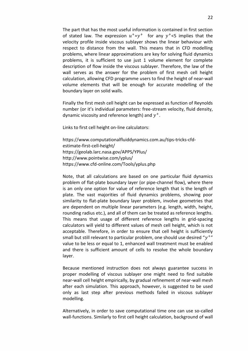
Wall functions are not applicable for cases with flow separation as shown in Figure 9.

Figure 9. Wall functions are not applicable to problems involving a flow separation.

More information regarding the “𝑦+” and first cell height estimation can be found via following link: https://www.computationalfluiddynamics.com.au/tag/wall-functions/

2.3.2 Introduction to RANS models

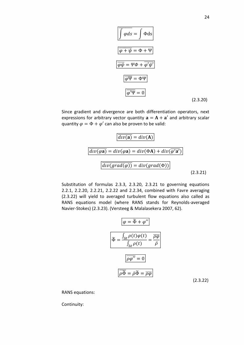
Recalling formulas 2.3.3, 2.3.4, 2.3.5, 2.3.6, 2.3.7 and 2.3.12 one can show that next expressions for derivatives and integrals for arbitrary scalar properties 𝜑 and 𝜓 hold:

𝜑′ = 𝜓′ = 0

Φ = Φ

𝜕𝜑

𝜕𝑠

=

𝜕Φ

𝜕𝑠

24

∫𝜑𝑑𝑠

= ∫Φds

𝜑 + 𝜓 = Φ + Ψ

𝜑𝜓 = 𝛹𝛷 + 𝜑′𝜓′

𝜑Ψ = ΦΨ

𝜑′Ψ = 0

(2.3.20) Since gradient and divergence are both differentiation operators, next expressions for arbitrary vector quantity 𝐚 = 𝐀 + 𝐚′ and arbitrary scalar quantity 𝜑 = Φ + 𝜑′ can also be proven to be valid:

𝑑𝑖𝑣(𝐚) = 𝑑𝑖𝑣(𝐀)

𝑑𝑖𝑣(𝜑𝐚) = 𝑑𝑖𝑣(𝜑𝐚) = 𝑑𝑖𝑣(Φ𝐀) + 𝑑𝑖𝑣(𝜑′𝐚′ )

𝑑𝑖𝑣(𝑔𝑟𝑎𝑑(𝜑)) = 𝑑𝑖𝑣(𝑔𝑟𝑎𝑑(Φ))

(2.3.21) Substitution of formulas 2.3.3, 2.3.20, 2.3.21 to governing equations 2.2.1, 2.2.20, 2.2.21, 2.2.22 and 2.2.34, combined with Favre averaging (2.3.22) will yield to averaged turbulent flow equations also called as RANS equations model (where RANS stands for Reynolds-averaged Navier-Stokes) (2.3.23). (Versteeg & Malalasekera 2007, 62).

𝜑 = Φ + 𝜑′′

Φ =∫ 𝜌(𝑡)𝜑(𝑡)

∆𝑡

∫ 𝜌(𝑡)

∆𝑡

=𝜌𝜑

��

𝜌𝜑′′ = 0

𝜌Φ = ��Φ = 𝜌𝜑

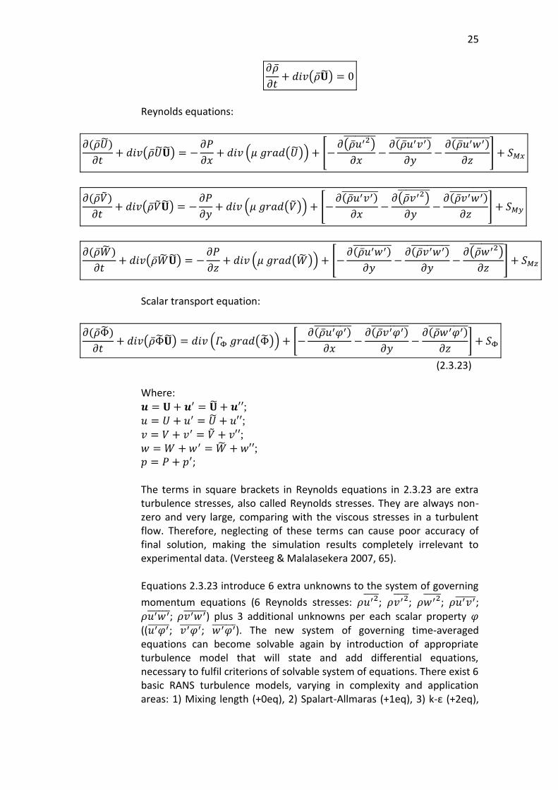
(2.3.22) RANS equations: Continuity:

25

𝜕��

𝜕𝑡+ 𝑑𝑖𝑣(��) = 0

Reynolds equations:

𝜕(��)

𝜕𝑡+ 𝑑𝑖𝑣(��) = −

𝜕𝑃

𝜕𝑥+ 𝑑𝑖𝑣 (𝜇 𝑔𝑟𝑎𝑑(��)) + [−

𝜕(��𝑢′2)

𝜕𝑥−

𝜕(��𝑢′𝑣′)

𝜕𝑦−

𝜕(��𝑢′𝑤′)

𝜕𝑧] + 𝑆𝑀𝑥

𝜕(��)

𝜕𝑡+ 𝑑𝑖𝑣(��) = −

𝜕𝑃

𝜕𝑦+ 𝑑𝑖𝑣 (𝜇 𝑔𝑟𝑎𝑑(��)) + [−

𝜕(��𝑢′𝑣′)

𝜕𝑥−

𝜕(��𝑣′2)

𝜕𝑦−

𝜕(��𝑣′𝑤′)

𝜕𝑧] + 𝑆𝑀𝑦

𝜕(��)

𝜕𝑡+ 𝑑𝑖𝑣(��) = −

𝜕𝑃

𝜕𝑧+ 𝑑𝑖𝑣 (𝜇 𝑔𝑟𝑎𝑑(��)) + [−

𝜕(��𝑢′𝑤′)

𝜕𝑦−

𝜕(��𝑣′𝑤′)

𝜕𝑦−

𝜕(��𝑤′2)

𝜕𝑧] + 𝑆𝑀𝑧

Scalar transport equation:

𝜕(��Φ)

𝜕𝑡+ 𝑑𝑖𝑣(��Φ��) = 𝑑𝑖𝑣 (𝛤Φ 𝑔𝑟𝑎𝑑(Φ)) + [−

𝜕(��𝑢′𝜑′)

𝜕𝑥−

𝜕(��𝑣′𝜑′)

𝜕𝑦−

𝜕(��𝑤′𝜑′)

𝜕𝑧] + 𝑆Φ

(2.3.23) Where: 𝒖 = 𝐔 + 𝒖′ = �� + 𝒖′′; 𝑢 = 𝑈 + 𝑢′ = �� + 𝑢′′; 𝑣 = 𝑉 + 𝑣′ = �� + 𝑣′′; 𝑤 = 𝑊 + 𝑤′ = �� + 𝑤′′; 𝑝 = 𝑃 + 𝑝′; The terms in square brackets in Reynolds equations in 2.3.23 are extra turbulence stresses, also called Reynolds stresses. They are always non-zero and very large, comparing with the viscous stresses in a turbulent flow. Therefore, neglecting of these terms can cause poor accuracy of final solution, making the simulation results completely irrelevant to experimental data. (Versteeg & Malalasekera 2007, 65). Equations 2.3.23 introduce 6 extra unknowns to the system of governing

momentum equations (6 Reynolds stresses: 𝜌𝑢′2 ; 𝜌𝑣′2 ; 𝜌𝑤′2 ; 𝜌𝑢′𝑣′ ; 𝜌𝑢′𝑤′ ; 𝜌𝑣′𝑤′ ) plus 3 additional unknowns per each scalar property 𝜑 ((𝑢′𝜑′ ; 𝑣′𝜑′ ; 𝑤′𝜑′ ). The new system of governing time-averaged equations can become solvable again by introduction of appropriate turbulence model that will state and add differential equations, necessary to fulfil criterions of solvable system of equations. There exist 6 basic RANS turbulence models, varying in complexity and application areas: 1) Mixing length (+0eq), 2) Spalart-Allmaras (+1eq), 3) k-ε (+2eq),

26

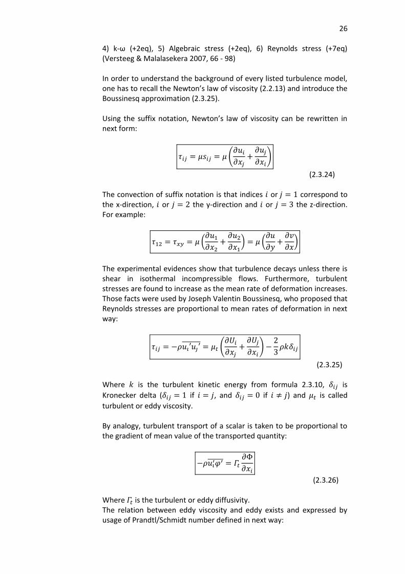
4) k-ω (+2eq), 5) Algebraic stress (+2eq), 6) Reynolds stress (+7eq) (Versteeg & Malalasekera 2007, 66 - 98) In order to understand the background of every listed turbulence model, one has to recall the Newton’s law of viscosity (2.2.13) and introduce the Boussinesq approximation (2.3.25). Using the suffix notation, Newton’s law of viscosity can be rewritten in next form:

𝜏𝑖𝑗 = 𝜇𝑠𝑖𝑗 = 𝜇 (𝜕𝑢𝑖

𝜕𝑥𝑗+

𝜕𝑢𝑗

𝜕𝑥𝑖)

(2.3.24) The convection of suffix notation is that indices 𝑖 or 𝑗 = 1 correspond to the x-direction, 𝑖 or 𝑗 = 2 the y-direction and 𝑖 or 𝑗 = 3 the z-direction. For example:

𝜏12 = 𝜏𝑥𝑦 = 𝜇 (𝜕𝑢1

𝜕𝑥2+

𝜕𝑢2

𝜕𝑥1) = 𝜇 (

𝜕𝑢

𝜕𝑦+

𝜕𝑣

𝜕𝑥)

The experimental evidences show that turbulence decays unless there is shear in isothermal incompressible flows. Furthermore, turbulent stresses are found to increase as the mean rate of deformation increases. Those facts were used by Joseph Valentin Boussinesq, who proposed that Reynolds stresses are proportional to mean rates of deformation in next way:

𝜏𝑖𝑗 = −𝜌𝑢𝑖′𝑢𝑗′ = 𝜇𝑡 (𝜕𝑈𝑖

𝜕𝑥𝑗+

𝜕𝑈𝑗

𝜕𝑥𝑖) −

2

3𝜌𝑘𝛿𝑖𝑗

(2.3.25) Where 𝑘 is the turbulent kinetic energy from formula 2.3.10, 𝛿𝑖𝑗 is

Kronecker delta (𝛿𝑖𝑗 = 1 if 𝑖 = 𝑗, and 𝛿𝑖𝑗 = 0 if 𝑖 ≠ 𝑗) and 𝜇𝑡 is called

turbulent or eddy viscosity. By analogy, turbulent transport of a scalar is taken to be proportional to the gradient of mean value of the transported quantity:

−𝜌𝑢𝑖′𝜑′ = 𝛤𝑡

𝜕Φ

𝜕𝑥𝑖

(2.3.26) Where 𝛤𝑡 is the turbulent or eddy diffusivity. The relation between eddy viscosity and eddy exists and expressed by usage of Prandtl/Schmidt number defined in next way:

27

𝜎𝑡 =𝜇𝑡

𝛤𝑡

(2.3.27) Various flow experiments confirm that value 𝜎𝑡 is constant, and hence most of free and commercial CFD software set the value 𝜎𝑡 = 1. (Versteeg & Malalasekera 2007, 68).

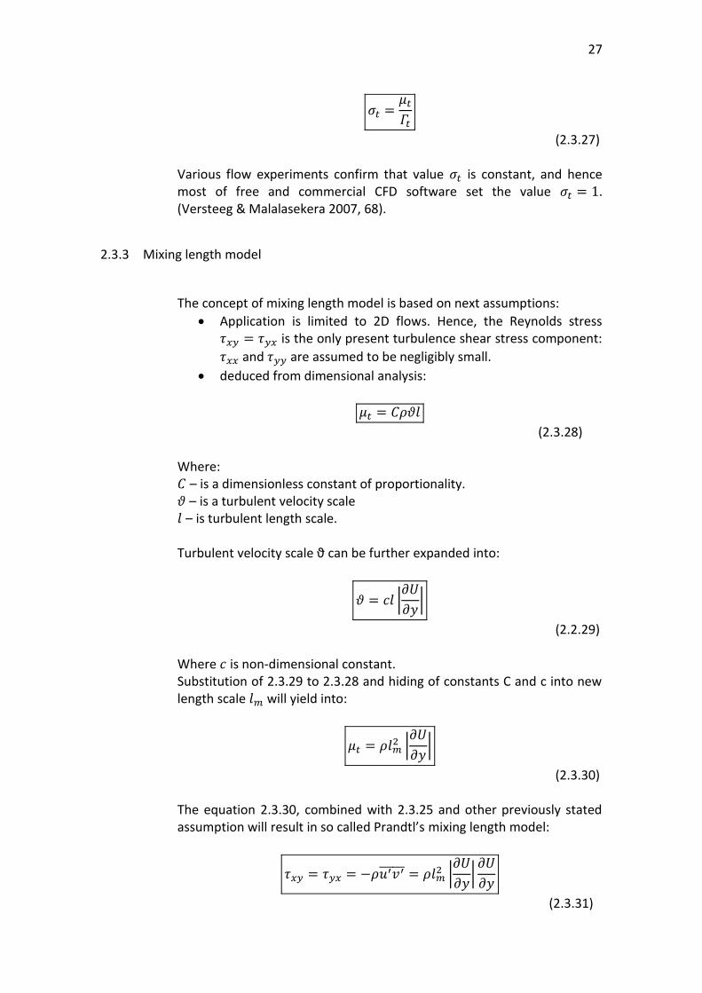
2.3.3 Mixing length model

The concept of mixing length model is based on next assumptions:

Application is limited to 2D flows. Hence, the Reynolds stress 𝜏𝑥𝑦 = 𝜏𝑦𝑥 is the only present turbulence shear stress component:

𝜏𝑥𝑥 and 𝜏𝑦𝑦 are assumed to be negligibly small.

deduced from dimensional analysis:

𝜇𝑡 = 𝐶𝜌𝜗𝑙

(2.3.28) Where: 𝐶 – is a dimensionless constant of proportionality. 𝜗 – is a turbulent velocity scale 𝑙 – is turbulent length scale. Turbulent velocity scale ϑ can be further expanded into:

𝜗 = 𝑐𝑙 |𝜕𝑈

𝜕𝑦|

(2.2.29) Where 𝑐 is non-dimensional constant. Substitution of 2.3.29 to 2.3.28 and hiding of constants C and c into new length scale 𝑙𝑚 will yield into:

𝜇𝑡 = 𝜌𝑙𝑚2 |

𝜕𝑈

𝜕𝑦|

(2.3.30) The equation 2.3.30, combined with 2.3.25 and other previously stated assumption will result in so called Prandtl’s mixing length model:

𝜏𝑥𝑦 = 𝜏𝑦𝑥 = −𝜌𝑢′𝑣′ = 𝜌𝑙𝑚2 |

𝜕𝑈

𝜕𝑦|𝜕𝑈

𝜕𝑦

(2.3.31)

28

The same approach, applied to turbulent transport of arbitrary scalar quantity will yield into:

−𝜌𝑣′𝜑′ = 𝛤𝑡

𝜕Φ

𝜕𝑦

(2.3.32) The Mixing length model finally allows to define unknown Reynolds stresses for 2D flows with no additional equations (Therefore it’s also called 0-equation model). The only things that must be the object consideration are values of 𝑙𝑚 and 𝜎𝑡. The specification of these values can be found in book of H. K. Versteeg, W. Malalasekera “An Introduction to Computational Fluid Dynamics, The Finite Volume Method” second edition, pages 70. Advantages of the Mixing length model:

easy and inexpensive implementation

sufficiently accurate predictions for thin shear layers: jets, mixing layers, wakes and boundary layers

well established Disadvantages:

completely incapable of modelling flows with separation and re-circulation

completely incapable of describing flows with separation and re-circulation

2.3.4 k-ε model

The standard k-ε model provides an acceptable compromise between reliability, computational costs and accuracy, what makes k-ε model to be apparently the most popular turbulence model, used in industry. This is a semi-empirical 2-equation eddy-viscosity model, solving 2 additional equations for turbulent kinetic energy “𝑘” (2.3.10) and rate of energy dissipation per unit volume “휀”. To understand the concept of k-ε, one has to introduce the concept of the mean kinetic energy “𝐾” and the instantaneous kinetic energy “𝑘(𝑡)”, that are defined in next way:

𝐾 =1

2(𝑈2 + 𝑉2 + 𝑊2)

(2.3.33)

29

𝑘(𝑡) = 𝐾 + 𝑘

(2.3.34) Another prerequisite for further model description is the decomposition of deformation rate tensor “𝑠𝑖𝑗” to average and fluctuating part. Recalling

formula 2.2.12, one can show that decomposition of “𝑠𝑖𝑗” will hold as

follows:

𝑠𝑖𝑗 = 𝑆𝑖𝑗 + 𝑠′𝑖𝑗 =

1

2[𝜕𝑈𝑖

𝜕𝑥𝑗+

𝜕𝑈𝑗

𝜕𝑥𝑖] +

1

2[𝜕𝑢′

𝑖

𝜕𝑥𝑗+

𝜕𝑢′𝑗

𝜕𝑥𝑖]

(2.3.35) The scalar product of two tensors “𝑎𝑖𝑗” and “𝑏𝑖𝑗” is defined as follows:

𝑎𝑖𝑗 . 𝑏𝑖𝑗 = 𝑎11𝑏11 + 𝑎12𝑏12 + 𝑎13𝑏13 + 𝑎21𝑏21 + 𝑎22𝑏22 + 𝑎23𝑏23 + 𝑎31𝑏31 + 𝑎32𝑏32 + 𝑎33𝑏33

It can be shown that governing equations for mean flow kinetic energy “𝐾” (2.3.36) and for turbulent kinetic energy “𝑘” (2.3.37) will take next form:

𝜕(𝜌𝐾)

𝜕𝑡+ 𝑑𝑖𝑣(𝜌𝐾𝐔) = 𝑑𝑖𝑣(−𝑃𝐔 + 2𝜇𝐔𝑆𝑖𝑗 − 𝜌𝐔𝑢′

𝑖𝑢′𝑗

) − 2𝜇𝑆𝑖𝑗 . 𝑆𝑖𝑗 + 𝜌𝑢′𝑖𝑢′

𝑗 . 𝑆𝑖𝑗

(2.3.36)

𝜕(𝜌𝑘)

𝜕𝑡+ 𝑑𝑖𝑣(𝜌𝑘𝐔) = 𝑑𝑖𝑣 (−𝑝′𝐮′ + 2𝜇𝐮′𝑠′𝑖𝑗 − 𝜌

1

2𝑢′𝑖 . 𝑢′

𝑖𝑢′𝑗

) − 2𝜇𝑠′𝑖𝑗 . 𝑠′

𝑖𝑗 + 𝜌𝑢′

𝑖𝑢′𝑗

. 𝑆𝑖𝑗

(2.3.37) The second term on RHS of 2.3.37 is usually written as product of density “𝜌” and the rate of dissipation of turbulent kinetic energy per unit mass “휀”. Therefore “휀” is defined as follows:

휀 = 2𝜇

𝜌𝑠′

𝑖𝑗 . 𝑠′𝑖𝑗

(2.3.38) It is also possible to derive the exact differential governing equation for “휀”, but it contains many unknowns, and hence the standard k-ε model is based on next assumptions for velocity scale “𝜗” and length scale “𝑙”:

𝜗 = 𝑘1/2

(2.3.39)

30

𝑙 =𝑘3/2

휀

(2.3.40) The substitution of 2.3.39 and 2.3.40 to formula of eddy viscosity will give next relation:

𝜇𝑡 = 𝐶𝜌𝜗𝑙 = 𝜌𝐶𝜇

𝑘2

휀

(2.3.41) Where “𝐶𝜇” – is a dimensionless constant.

The formula 2.3.41 itself is an assumption of isotropic eddy viscosity, allowing to state two transport equations of standard k-ε model:

𝜕(𝜌𝑘)

𝜕𝑡+ 𝑑𝑖𝑣(𝜌𝑘𝐔) = 𝑑𝑖𝑣 [

𝜇𝑡

𝜎𝑘 𝑔𝑟𝑎𝑑(𝑘)] + 2𝜇𝑡𝑆𝑖𝑗 . 𝑆𝑖𝑗 − 𝜌휀

(2.3.42)

𝜕(𝜌휀)

𝜕𝑡+ 𝑑𝑖𝑣(𝜌휀𝐔) = 𝑑𝑖𝑣 [

𝜇𝑡

𝜎𝜀 𝑔𝑟𝑎𝑑(휀)] + 𝐶1𝜀

휀

𝑘2𝜇𝑡𝑆𝑖𝑗 . 𝑆𝑖𝑗 − 𝐶2𝜀

휀2

𝑘

(2.3.43) Where 𝐶𝜇 = 0.09; 𝜎𝑘 = 1; 𝜎𝜀 = 1.3; 𝐶1𝜀 = 1.44; 𝐶2𝜀 = 1.92 – are

empirically defined dimensionless constants, suitable for wide range of flows. The Reynolds stresses are found, using following Boussinesq approximation:

−𝜌𝑢′𝑖𝑢′

𝑗 = 𝜇𝑡 (

𝜕𝑈𝑖

𝜕𝑥𝑗+

𝜕𝑈𝑗

𝜕𝑥𝑖) −

2

3𝜌𝑘𝛿𝑖𝑗 = 2𝜇𝑡𝑆𝑖𝑗 −

2

3𝜌𝑘𝛿𝑖𝑗

In order to run k-ε model appropriately, some CFD codes in addition to turbulence intensity might also ask to specify the values of “𝑘” and ”휀” for system inlet. This can be done either by reviewing literature, covering particular cases of study, which is more preferable option, or using next formulas, connecting “𝑘” and ”ε” with turbulence intensity “𝑇𝑖” and length scale “𝑙”:

𝑘 =2

3(𝑈𝑟𝑒𝑓𝑇𝑖)

2

(2.3.44)

31

휀 = 𝐶𝜇3/4 𝑘3/2

𝑙

(2.3.45)

𝑙 = 0.07𝐿

(2.3.46) Where “𝐿” – is a characteristic length of equipment (equivalent pipe diameter). (Versteeg & Malalasekera 2007, 72 - 88). Equivalent pipe diameter on-line calculator with some explanation theory: http://www.engineeringtoolbox.com/equivalent-diameter-d_205.html In cases, when equivalent pipe diameter is not obvious to define it’s sufficient either to use default settings in CFD code (if exist) or arbitrary finite and small values for “휀”. (Versteeg & Malalasekera 2007, 77). In addition to standard k-ε (SKE) most of free and commercial CFD codes provide users with two more advanced variants of k-ε model: k-ε RNG (Renormalization Groups) and k-ε RKE (Realizable). k-ε RNG model instead of using empirically defined constants 𝐶𝜇; 𝜎𝑘; 𝜎𝜀; 𝐶1𝜀; 𝐶2𝜀 resolves them using statistical methods, making it

more precise for wider range of more complex flows. k-ε RKE model is an improvement of standard k-ε model, varying in next points:

k-ε RKE contains a new formulation for the turbulent viscosity with varying parameter “𝐶𝜇” that was assumed to be constant for

standard k-ε model.

A new transport equation for the dissipation rate “ɛ” is derived from exact transport equation of the mean-square vorticity fluctuation.

Unlike k-ε SKE or k-ε RNG, k-ε RKE model satisfies several constraints of physics of turbulent flows, making RKE potentially the most accurate variation of k-ε model. Note that all k-ε models variation are preferred to use only for fully turbulent flows (high Reynolds numbers), due to fully turbulent flow assumption as a basement of the whole model. In addition to k-ε, there also exist other two-equation models such as Wilcox k-ω, Menter SST k-ω, algebraic stress equation model and non-linear k-ε. (Versteeg & Malalasekera 2007, 90 - 95). Unlike k-ε SKE, k-ε RNG or k-ε RKE, Wilcox k-ω shows the best performance for flows with low Reynolds numbers and very accurate results for flows in near-wall regions. It’s success in near-wall computations even yielded to creation of hybrid Menter SST k-ω model,

32

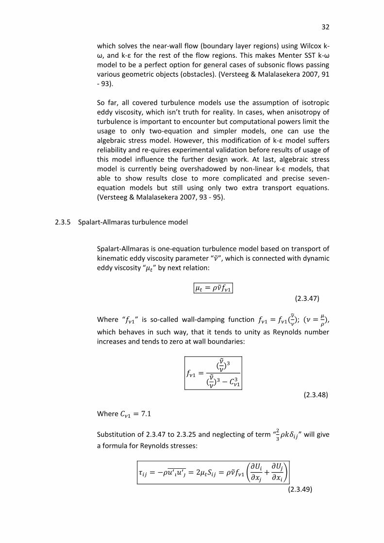
which solves the near-wall flow (boundary layer regions) using Wilcox k-ω, and k-ε for the rest of the flow regions. This makes Menter SST k-ω model to be a perfect option for general cases of subsonic flows passing various geometric objects (obstacles). (Versteeg & Malalasekera 2007, 91 - 93). So far, all covered turbulence models use the assumption of isotropic eddy viscosity, which isn’t truth for reality. In cases, when anisotropy of turbulence is important to encounter but computational powers limit the usage to only two-equation and simpler models, one can use the algebraic stress model. However, this modification of k-ε model suffers reliability and re-quires experimental validation before results of usage of this model influence the further design work. At last, algebraic stress model is currently being overshadowed by non-linear k-ε models, that able to show results close to more complicated and precise seven-equation models but still using only two extra transport equations. (Versteeg & Malalasekera 2007, 93 - 95).

2.3.5 Spalart-Allmaras turbulence model

Spalart-Allmaras is one-equation turbulence model based on transport of kinematic eddy viscosity parameter “𝜈”, which is connected with dynamic eddy viscosity “𝜇𝑡” by next relation:

𝜇𝑡 = 𝜌𝜈𝑓𝜈1

(2.3.47)

Where “𝑓𝜈1” is so-called wall-damping function 𝑓𝜈1 = 𝑓𝜈1(��

𝜈); (𝜈 =

𝜇

𝜌),

which behaves in such way, that it tends to unity as Reynolds number increases and tends to zero at wall boundaries:

𝑓𝜈1 =(𝜈𝜈)3

(𝜈𝜈)3 − 𝐶𝜈1

3

(2.3.48) Where 𝐶𝜈1 = 7.1

Substitution of 2.3.47 to 2.3.25 and neglecting of term “2

3𝜌𝑘𝛿𝑖𝑗” will give

a formula for Reynolds stresses:

𝜏𝑖𝑗 = −𝜌𝑢′𝑖𝑢′

𝑗 = 2𝜇𝑡𝑆𝑖𝑗 = 𝜌𝜈𝑓𝜈1 (

𝜕𝑈𝑖

𝜕𝑥𝑗+

𝜕𝑈𝑗

𝜕𝑥𝑖)

(2.3.49)

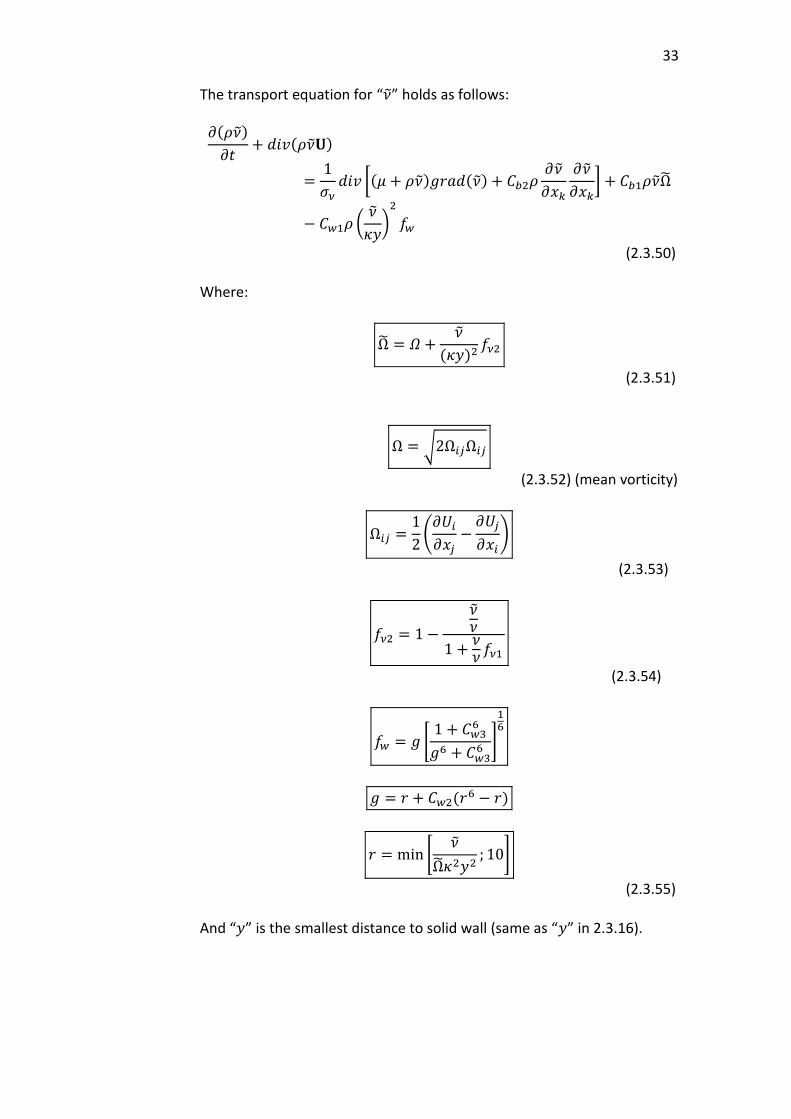
33

The transport equation for “𝜈” holds as follows: 𝜕(𝜌𝜈)

𝜕𝑡+ 𝑑𝑖𝑣(𝜌𝜈𝐔)

=1

𝜎𝜈𝑑𝑖𝑣 [(𝜇 + 𝜌𝜈)𝑔𝑟𝑎𝑑(𝜈) + 𝐶𝑏2𝜌

𝜕𝜈

𝜕𝑥𝑘

𝜕𝜈

𝜕𝑥𝑘] + 𝐶𝑏1𝜌𝜈Ω

− 𝐶𝑤1𝜌 (𝜈

𝜅𝑦)

2

𝑓𝑤

(2.3.50) Where:

Ω = 𝛺 +𝜈

(𝜅𝑦)2𝑓𝜈2

(2.3.51)

Ω = √2Ω𝑖𝑗Ω𝑖𝑗

(2.3.52) (mean vorticity)

Ω𝑖𝑗 =1

2(𝜕𝑈𝑖

𝜕𝑥𝑗−

𝜕𝑈𝑗

𝜕𝑥𝑖)

(2.3.53)

𝑓𝜈2 = 1 −

𝜈𝜈

1 +𝜈𝜈 𝑓𝜈1

(2.3.54)

𝑓𝑤 = 𝑔 [1 + 𝐶𝑤3

6

𝑔6 + 𝐶𝑤36 ]

16

𝑔 = 𝑟 + 𝐶𝑤2(𝑟6 − 𝑟)

𝑟 = min [𝜈

Ω𝜅2𝑦2; 10]

(2.3.55) And “𝑦” is the smallest distance to solid wall (same as “𝑦” in 2.3.16).

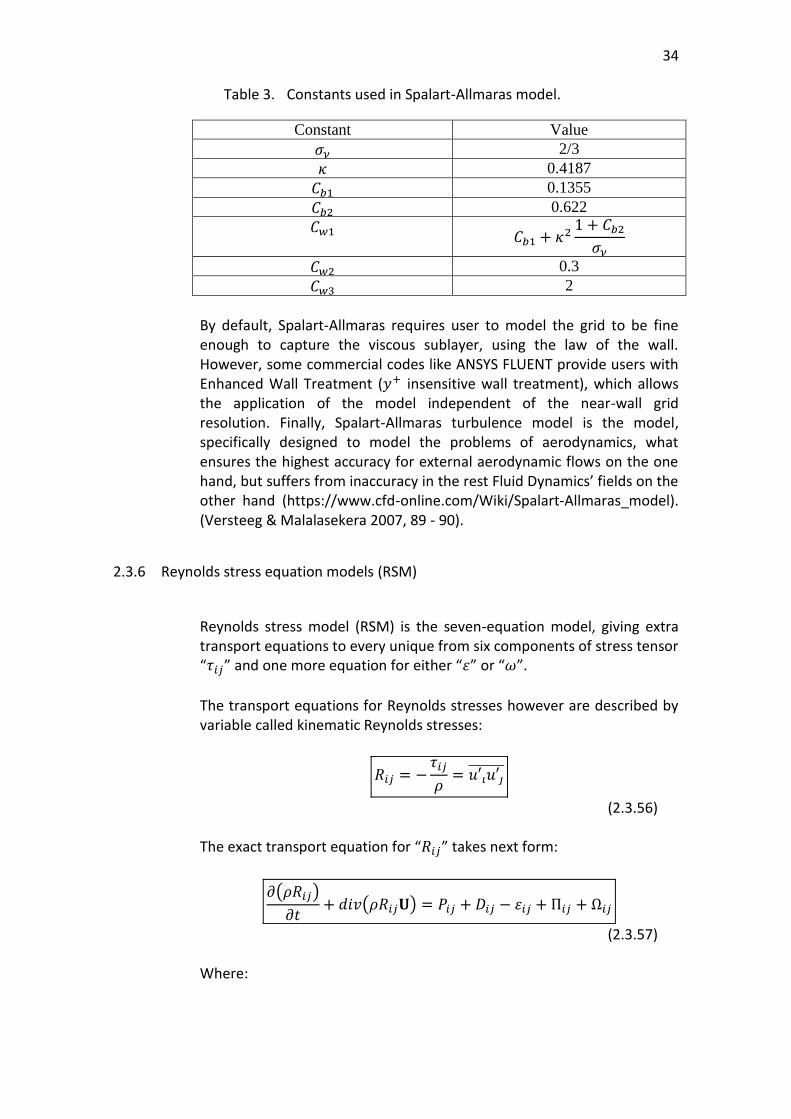
34

Table 3. Constants used in Spalart-Allmaras model.

Constant Value

𝜎𝜈 2/3

𝜅 0.4187

𝐶𝑏1 0.1355

𝐶𝑏2 0.622

𝐶𝑤1 𝐶𝑏1 + 𝜅2

1 + 𝐶𝑏2

𝜎𝜈

𝐶𝑤2 0.3

𝐶𝑤3 2

By default, Spalart-Allmaras requires user to model the grid to be fine enough to capture the viscous sublayer, using the law of the wall. However, some commercial codes like ANSYS FLUENT provide users with Enhanced Wall Treatment (𝑦+ insensitive wall treatment), which allows the application of the model independent of the near-wall grid resolution. Finally, Spalart-Allmaras turbulence model is the model, specifically designed to model the problems of aerodynamics, what ensures the highest accuracy for external aerodynamic flows on the one hand, but suffers from inaccuracy in the rest Fluid Dynamics’ fields on the other hand (https://www.cfd-online.com/Wiki/Spalart-Allmaras_model). (Versteeg & Malalasekera 2007, 89 - 90).

2.3.6 Reynolds stress equation models (RSM)

Reynolds stress model (RSM) is the seven-equation model, giving extra transport equations to every unique from six components of stress tensor “𝜏𝑖𝑗” and one more equation for either “휀” or “𝜔”.

The transport equations for Reynolds stresses however are described by variable called kinematic Reynolds stresses:

𝑅𝑖𝑗 = −𝜏𝑖𝑗

𝜌= 𝑢′𝑖𝑢′𝑗

(2.3.56) The exact transport equation for “𝑅𝑖𝑗” takes next form:

𝜕(𝜌𝑅𝑖𝑗)

𝜕𝑡+ 𝑑𝑖𝑣(𝜌𝑅𝑖𝑗𝐔) = 𝑃𝑖𝑗 + 𝐷𝑖𝑗 − 휀𝑖𝑗 + Π𝑖𝑗 + Ω𝑖𝑗

(2.3.57) Where:

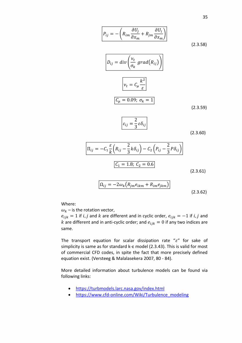
35

𝑃𝑖𝑗 = −(𝑅𝑖𝑚

𝜕𝑈𝑗

𝜕𝑥𝑚+ 𝑅𝑗𝑚

𝜕𝑈𝑖

𝜕𝑥𝑚)

(2.3.58)

𝐷𝑖𝑗 = 𝑑𝑖𝑣 (𝜈𝑡

𝜎𝑘 𝑔𝑟𝑎𝑑(𝑅𝑖𝑗))

𝜈𝑡 = 𝐶𝜇

𝑘2

휀

𝐶𝜇 = 0.09; 𝜎𝑘 = 1

(2.3.59)

휀𝑖𝑗 =2

3휀𝛿𝑖𝑗

(2.3.60)

Π𝑖𝑗 = −𝐶1

휀

𝑘(𝑅𝑖𝑗 −

2

3𝑘𝛿𝑖𝑗) − 𝐶2 (𝑃𝑖𝑗 −

2

3𝑃𝛿𝑖𝑗)

𝐶1 = 1.8; 𝐶2 = 0.6

(2.3.61)

Ω𝑖𝑗 = −2𝜔𝑘(𝑅𝑗𝑚𝑒𝑖𝑘𝑚 + 𝑅𝑖𝑚𝑒𝑗𝑘𝑚)

(2.3.62) Where: 𝜔𝑘 – is the rotation vector, 𝑒𝑖𝑗𝑘 = 1 if 𝑖, 𝑗 and 𝑘 are different and in cyclic order, 𝑒𝑖𝑗𝑘 = −1 if 𝑖, 𝑗 and

𝑘 are different and in anti-cyclic order; and 𝑒𝑖𝑗𝑘 = 0 if any two indices are

same. The transport equation for scalar dissipation rate “휀” for sake of simplicity is same as for standard k-ε model (2.3.43). This is valid for most of commercial CFD codes, in spite the fact that more precisely defined equation exist. (Versteeg & Malalasekera 2007, 80 - 84). More detailed information about turbulence models can be found via following links:

https://turbmodels.larc.nasa.gov/index.html

https://www.cfd-online.com/Wiki/Turbulence_modeling

https://turbmodels.larc.nasa.gov/index.html

https://www.cfd-online.com/Wiki/Turbulence_modeling

36

2.3.7 Direct Numerical Simulation (DNS) and Large Eddy Simulation (LES)

In Direct Numerical Simulation system of governing transient equations 2.2.1, 2.2.20, 2.2.21 and 2.2.22 solved directly without implementation of any turbulence model and Reynolds averaging at all (not a RANS model). As a consequence, DNS demands extremely fine mesh an sufficiently small time steps in order of simulate the motion of eddies with smallest size and highest rotational frequencies. Therefore, DNS demands computational powers that can be only satisfied by modern supercomputers, making this method unsuitable for commercial usage. And even usage of supercomputers so far haven’t allowed to use this method on complex geometries with highly turbulent flows. Finally, at the moment DNS can be applied only to incompressible, simple-geometry and low-Reynolds-number flows. In spite such limitations, scientists came up with computational technique called Large Eddy Simulation (LES), that can be considered as simplification of DNS applicable for conventional computers, allowing to use coarser meshing (not a RANS model too). The ideas behind LES are two empirically proven facts:

Most of kinetic turbulent energy is contained in largest eddies in flow, meaning that smaller eddies play relatively negligible role in turbulence effects.

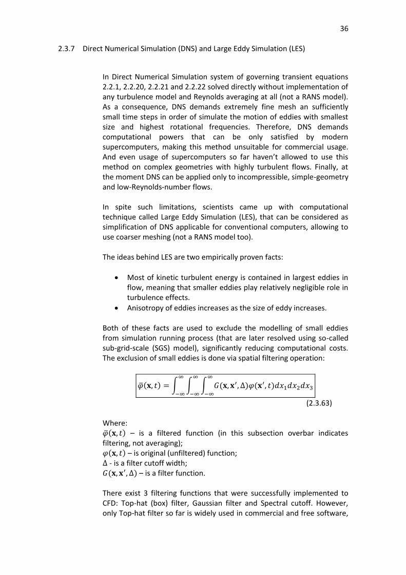
Anisotropy of eddies increases as the size of eddy increases. Both of these facts are used to exclude the modelling of small eddies from simulation running process (that are later resolved using so-called sub-grid-scale (SGS) model), significantly reducing computational costs. The exclusion of small eddies is done via spatial filtering operation:

��(𝐱, 𝑡) = ∫ ∫ ∫ 𝐺(𝐱, 𝐱′, ∆)𝜑(𝐱′, 𝑡)𝑑𝑥1𝑑𝑥2𝑑𝑥3

∞

−∞

∞

−∞

∞

−∞

(2.3.63) Where: ��(𝐱, 𝑡) – is a filtered function (in this subsection overbar indicates filtering, not averaging); 𝜑(𝐱, 𝑡) – is original (unfiltered) function; ∆ - is a filter cutoff width; 𝐺(𝐱, 𝐱′, ∆) – is a filter function. There exist 3 filtering functions that were successfully implemented to CFD: Top-hat (box) filter, Gaussian filter and Spectral cutoff. However, only Top-hat filter so far is widely used in commercial and free software,

37

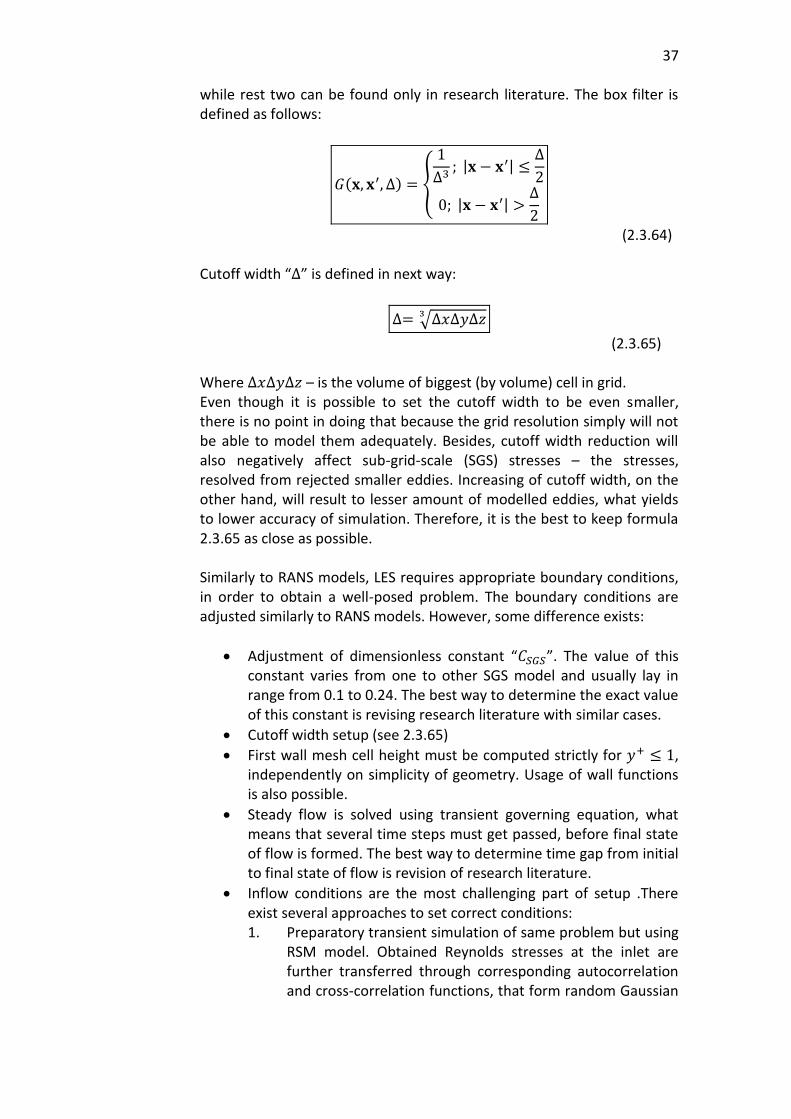
while rest two can be found only in research literature. The box filter is defined as follows:

𝐺(𝐱, 𝐱′, ∆) = {

1

∆3; |𝐱 − 𝐱′| ≤

∆

2

0; |𝐱 − 𝐱′| >∆

2

(2.3.64) Cutoff width “∆” is defined in next way:

∆= √∆𝑥∆𝑦∆𝑧3

(2.3.65) Where ∆𝑥∆𝑦∆𝑧 – is the volume of biggest (by volume) cell in grid. Even though it is possible to set the cutoff width to be even smaller, there is no point in doing that because the grid resolution simply will not be able to model them adequately. Besides, cutoff width reduction will also negatively affect sub-grid-scale (SGS) stresses – the stresses, resolved from rejected smaller eddies. Increasing of cutoff width, on the other hand, will result to lesser amount of modelled eddies, what yields to lower accuracy of simulation. Therefore, it is the best to keep formula 2.3.65 as close as possible. Similarly to RANS models, LES requires appropriate boundary conditions, in order to obtain a well-posed problem. The boundary conditions are adjusted similarly to RANS models. However, some difference exists:

Adjustment of dimensionless constant “𝐶𝑆𝐺𝑆”. The value of this constant varies from one to other SGS model and usually lay in range from 0.1 to 0.24. The best way to determine the exact value of this constant is revising research literature with similar cases.

Cutoff width setup (see 2.3.65)

First wall mesh cell height must be computed strictly for 𝑦+ ≤ 1, independently on simplicity of geometry. Usage of wall functions is also possible.

Steady flow is solved using transient governing equation, what means that several time steps must get passed, before final state of flow is formed. The best way to determine time gap from initial to final state of flow is revision of research literature.

Inflow conditions are the most challenging part of setup .There exist several approaches to set correct conditions: 1. Preparatory transient simulation of same problem but using

RSM model. Obtained Reynolds stresses at the inlet are further transferred through corresponding autocorrelation and cross-correlation functions, that form random Gaussian

38

perturbations, to LES

2. Extension of computational domain. Long upstream distances are required in order to ensure the generation of fully developed flow from turbulence-free reservoirs

3. Direct specification of shear stresses and velocity profiles in inlet. (Versteeg & Malalasekera 2007, 98 - 114).

39

2.4 Finite volume method and solution schemes

2.4.1 Finite volume method for diffusion problems

Pure diffusion problems are one of the easiest problems that finite volume method can handle. In physics and engineering pure diffusion problems mostly involve problems of heat transfer in solids. In spite the fact that pure diffusion model is not sufficient for fluids due to involvement of convection, discretization procedure for solids and fluids is similar. There-fore in this section problems of pure steady-state diffusion will be covered first, and convection-diffusion problems with pressure-velocity coupling later. Pure diffusion equation for three-dimensional problems is written as follows:

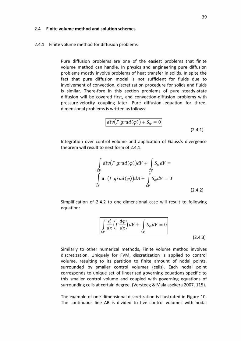
𝑑𝑖𝑣(𝛤 𝑔𝑟𝑎𝑑(𝜑)) + 𝑆𝜑 = 0

(2.4.1) Integration over control volume and application of Gauss’s divergence theorem will result to next form of 2.4.1:

∫𝑑𝑖𝑣(𝛤 𝑔𝑟𝑎𝑑(𝜑))𝑑𝑉

𝐶𝑉


𝐶𝑉

=

∫ 𝐧 . (𝛤 𝑔𝑟𝑎𝑑(𝜑))𝑑𝐴

𝐶𝑆


𝐶𝑉

= 0

(2.4.2) Simplification of 2.4.2 to one-dimensional case will result to following equation:

∫𝑑

𝑑𝑥(𝛤

𝑑𝜑

𝑑𝑥) 𝑑𝑉

𝐶𝑉


𝐶𝑉

= 0

(2.4.3) Similarly to other numerical methods, Finite volume method involves discretization. Uniquely for FVM, discretization is applied to control volume, resulting to its partition to finite amount of nodal points, surrounded by smaller control volumes (cells). Each nodal point corresponds to unique set of linearized governing equations specific to this smaller control volume and coupled with governing equations of surrounding cells at certain degree. (Versteeg & Malalasekera 2007, 115). The example of one-dimensional discretization is illustrated in Figure 10. The continuous line AB is divided to five control volumes with nodal

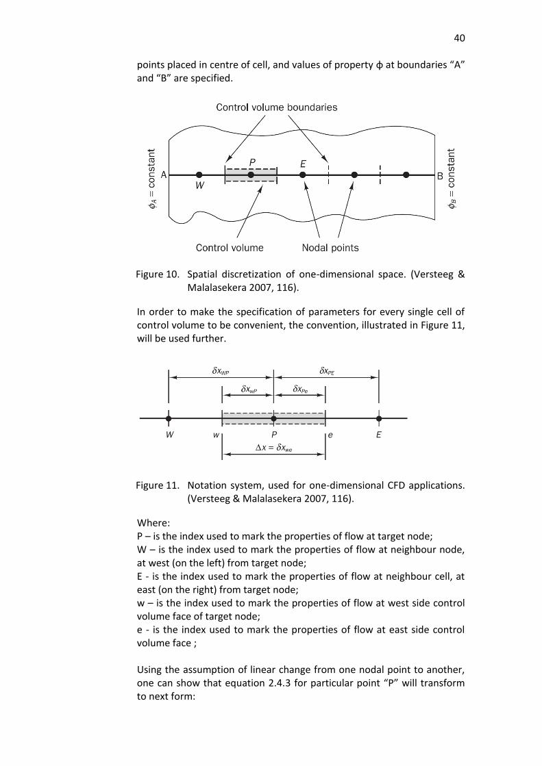
40

points placed in centre of cell, and values of property φ at boundaries “A” and “B” are specified.

Figure 10. Spatial discretization of one-dimensional space. (Versteeg & Malalasekera 2007, 116).

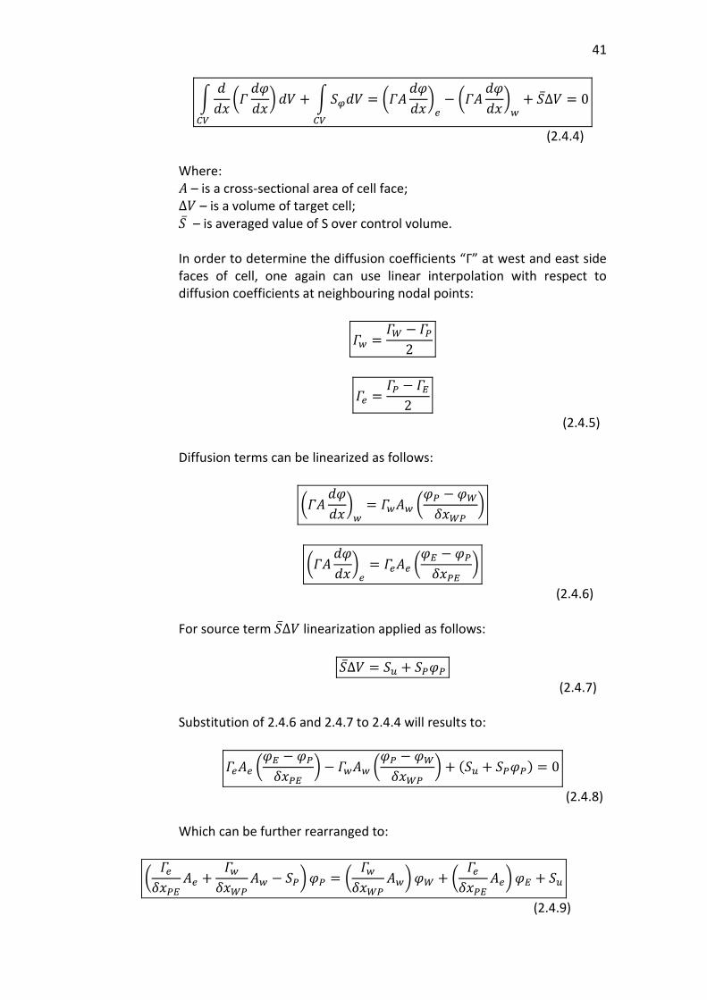
In order to make the specification of parameters for every single cell of control volume to be convenient, the convention, illustrated in Figure 11, will be used further.

Figure 11. Notation system, used for one-dimensional CFD applications. (Versteeg & Malalasekera 2007, 116).

Where: P – is the index used to mark the properties of flow at target node; W – is the index used to mark the properties of flow at neighbour node, at west (on the left) from target node; E - is the index used to mark the properties of flow at neighbour cell, at east (on the right) from target node; w – is the index used to mark the properties of flow at west side control volume face of target node; e - is the index used to mark the properties of flow at east side control volume face ; Using the assumption of linear change from one nodal point to another, one can show that equation 2.4.3 for particular point “P” will transform to next form:

41

∫𝑑

𝑑𝑥(𝛤

𝑑𝜑

𝑑𝑥)𝑑𝑉

𝐶𝑉

+ ∫ 𝑆𝜑𝑑𝑉

𝐶𝑉

= (𝛤𝐴𝑑𝜑

𝑑𝑥)

𝑒− (𝛤𝐴

𝑑𝜑

𝑑𝑥)𝑤

+ 𝑆∆𝑉 = 0

(2.4.4) Where: 𝐴 – is a cross-sectional area of cell face; ∆𝑉 – is a volume of target cell; 𝑆 – is averaged value of S over control volume. In order to determine the diffusion coefficients “Γ” at west and east side faces of cell, one again can use linear interpolation with respect to diffusion coefficients at neighbouring nodal points:

𝛤𝑤 =𝛤𝑊 − 𝛤𝑃

2

𝛤𝑒 =𝛤𝑃 − 𝛤𝐸

2

(2.4.5) Diffusion terms can be linearized as follows:

(𝛤𝐴𝑑𝜑

𝑑𝑥)𝑤

= 𝛤𝑤𝐴𝑤 (𝜑𝑃 − 𝜑𝑊

𝛿𝑥𝑊𝑃)

(𝛤𝐴𝑑𝜑

𝑑𝑥)𝑒

= 𝛤𝑒𝐴𝑒 (𝜑𝐸 − 𝜑𝑃

𝛿𝑥𝑃𝐸)

(2.4.6) For source term 𝑆∆𝑉 linearization applied as follows:

𝑆∆𝑉 = 𝑆𝑢 + 𝑆𝑃𝜑𝑃

(2.4.7) Substitution of 2.4.6 and 2.4.7 to 2.4.4 will results to:

𝛤𝑒𝐴𝑒 (𝜑𝐸 − 𝜑𝑃

𝛿𝑥𝑃𝐸) − 𝛤𝑤𝐴𝑤 (

𝜑𝑃 − 𝜑𝑊

𝛿𝑥𝑊𝑃) + (𝑆𝑢 + 𝑆𝑃𝜑𝑃) = 0

(2.4.8) Which can be further rearranged to:

(𝛤𝑒

𝛿𝑥𝑃𝐸𝐴𝑒 +

𝛤𝑤

𝛿𝑥𝑊𝑃𝐴𝑤 − 𝑆𝑃)𝜑𝑃 = (

𝛤𝑤

𝛿𝑥𝑊𝑃𝐴𝑤)𝜑𝑊 + (

𝛤𝑒

𝛿𝑥𝑃𝐸𝐴𝑒)𝜑𝐸 + 𝑆𝑢

(2.4.9)

42

The resulting equation 2.4.9 is a simple algebraic equation allowing to solve value “𝜑” for particular nodal point P. By refinement of the grid (adding the nodal points) one can solve “𝜑” with higher accuracy (“𝜑” ap-pears to be more specifically determined in control volume). On the other hand, mesh refinement yields to increased amount of algebraic equations (1 algebraic equation per nodal point), what results to increase size of corresponding matrix of system of algebraic equations, finally leading to in-creased computational time. The outcome of 2.4.9 can be further generalized to next form:

𝑎𝑃𝜑𝑃 = 𝑎𝑊𝜑𝑊 + 𝑎𝐸𝜑𝐸 + 𝑆𝑢

(2.4.10) With corresponding table for coefficients “a”:

Table 4. Coefficients “a” for 1D diffusion problems.

𝑎𝑊 𝑎𝐸 𝑎𝑃 𝛤𝑤𝐴𝑤

𝛿𝑥𝑊𝑃

𝛤𝑒𝐴𝑒

𝛿𝑥𝑃𝐸

𝑎𝑊 + 𝑎𝐸 + 𝑆𝑝

2.4.9 or 2.4.10 together with Table 4 form the mathematical model, sufficient to solve one-dimensional problems. However 1D diffusion models are rarely used in real engineering work due to insufficient accuracy especially in complex geometries. Therefore one has to extend existing methods for one-dimensional cases to two- and three-dimensional cases by adding extra terms to 2.4.10:

𝑎𝑃𝜑𝑃 = 𝑎𝑊𝜑𝑊 + 𝑎𝐸𝜑𝐸 + 𝑎𝑆𝜑𝑆 + 𝑎𝑁𝜑𝑁 + 𝑆𝑢

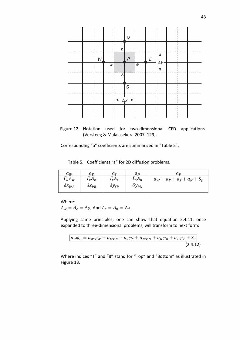
(2.4.11) Where indices “S” and “N” stand for southern and northern neighbouring nodal points according to Figure 12.

43

Figure 12. Notation used for two-dimensional CFD applications. (Versteeg & Malalasekera 2007, 129).

Corresponding “a” coefficients are summarized in “Table 5”.


𝑎𝑊 𝑎𝐸 𝑎𝑆 𝑎𝑁 𝑎𝑃 𝛤𝑤𝐴𝑤

𝛿𝑥𝑊𝑃

𝛤𝑒𝐴𝑒

𝛿𝑥𝑃𝐸

𝛤𝑠𝐴𝑠

𝛿𝑦𝑆𝑃

𝛤𝑛𝐴𝑛

𝛿𝑦𝑃𝑁

𝑎𝑊 + 𝑎𝐸 + 𝑎𝑆 + 𝑎𝑁 + 𝑆𝑝

Where: 𝐴𝑤 = 𝐴𝑒 = ∆𝑦; And 𝐴𝑠 = 𝐴𝑛 = ∆𝑥. Applying same principles, one can show that equation 2.4.11, once expanded to three-dimensional problems, will transform to next form:

𝑎𝑃𝜑𝑃 = 𝑎𝑊𝜑𝑊 + 𝑎𝐸𝜑𝐸 + 𝑎𝑆𝜑𝑆 + 𝑎𝑁𝜑𝑁 + 𝑎𝐵𝜑𝐵 + 𝑎𝑇𝜑𝑇 + 𝑆𝑢

(2.4.12) Where indices “T” and “B” stand for “Top” and “Bottom” as illustrated in Figure 13.

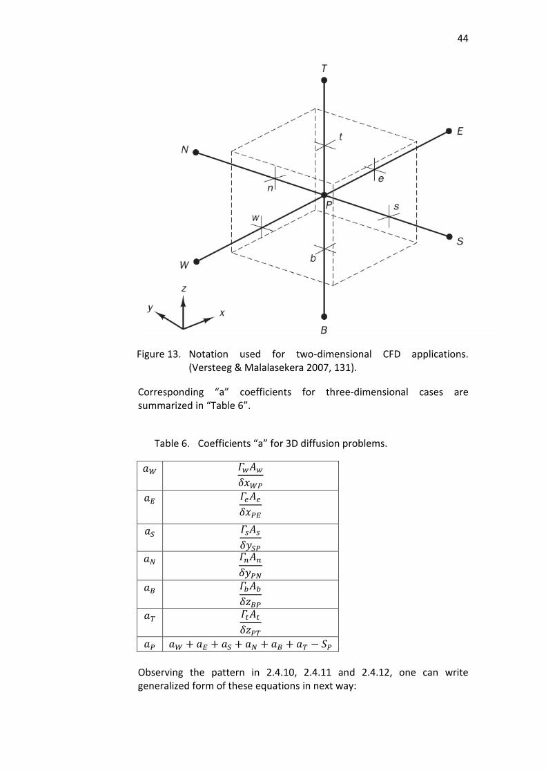
44

Figure 13. Notation used for two-dimensional CFD applications. (Versteeg & Malalasekera 2007, 131).

Corresponding “a” coefficients for three-dimensional cases are summarized in “Table 6”.


𝑎𝑊 𝛤𝑤𝐴𝑤

𝛿𝑥𝑊𝑃

𝑎𝐸 𝛤𝑒𝐴𝑒

𝛿𝑥𝑃𝐸

𝑎𝑆 𝛤𝑠𝐴𝑠

𝛿𝑦𝑆𝑃

𝑎𝑁 𝛤𝑛𝐴𝑛

𝛿𝑦𝑃𝑁

𝑎𝐵 𝛤𝑏𝐴𝑏

𝛿𝑧𝐵𝑃

𝑎𝑇 𝛤𝑡𝐴𝑡

𝛿𝑧𝑃𝑇

𝑎𝑃 𝑎𝑊 + 𝑎𝐸 + 𝑎𝑆 + 𝑎𝑁 + 𝑎𝐵 + 𝑎𝑇 − 𝑆𝑃

Observing the pattern in 2.4.10, 2.4.11 and 2.4.12, one can write generalized form of these equations in next way:

45

𝑎𝑃𝜑𝑃 = ∑ 𝑎𝑛𝑏𝜑𝑛𝑏 + 𝑆𝑢

(2.4.13) And,

𝑎𝑃 = ∑𝑎𝑛𝑏 − 𝑆𝑃

(2.4.14) Where index “nb” corresponds to neighbouring nodes relatively to target node. (Versteeg & Malalasekera 2007, 115 - 133).

2.4.2 Convection-diffusion problems

General form of convection-equation is read as follows:

∫𝐧 . (𝜌𝜑𝐮)𝑑𝐴

𝐴

= ∫𝐧 . (𝛤(𝑔𝑟𝑎𝑑(𝜑))𝑑𝐴

𝐴


𝐶𝑉

(2.4.15) Simplification of 2.4.15 to one-dimensional and neglecting of source term case will result to:

𝑑(𝜌𝑢𝜑)

𝑑𝑥=

𝑑

𝑑𝑥(𝛤 (

𝑑𝜑

𝑑𝑥))

(2.4.16) In addition to 2.4.16, one also has to consider the continuity equation:

𝑑(𝜌𝑢)

𝑑𝑥= 0

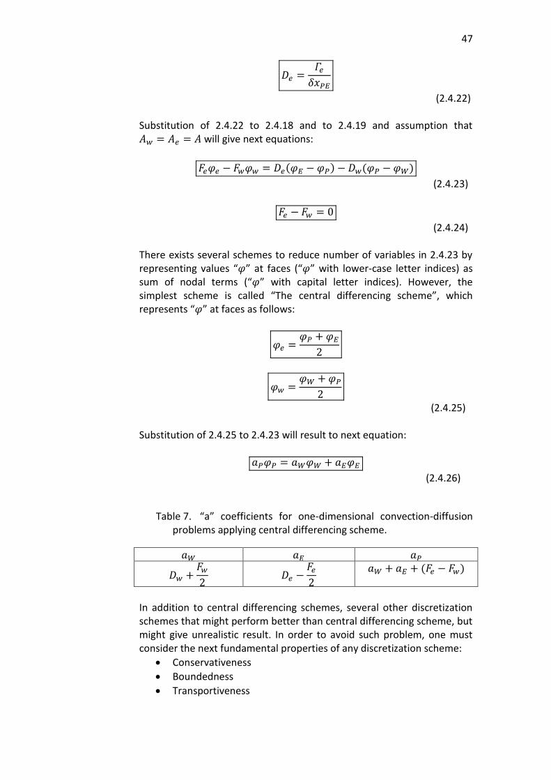
(2.4.17) To apply discretization to 2.4.16 and 2.4.17, the notation similar to diffusion problems, shown in Figure 14, is used with only difference of presence of velocity components “𝑢”, “𝑣” and “𝑤”.

46

Figure 14. Notation, used for one-dimensional convection-diffusion problems. (Versteeg & Malalasekera 2007, 135).

With given convention, one can transform equations 2.4.16 and 2.4.17 in linearized form:

(𝜌𝑢𝐴𝜑)𝑒 − (𝜌𝑢𝐴𝜑)𝑤 = (𝛤𝐴𝑑𝜑

𝑑𝑥)𝑒− (𝛤𝐴

𝑑𝜑

𝑑𝑥)𝑤

(2.4.18) For transport equation of “𝜑”, and for continuity equation:

(𝜌𝑢𝐴)𝑒 − (𝜌𝑢𝐴)𝑤 = 0

(2.4.19) For the sake of convenience, one can introduce next replacements for 2.4.18 and 2.4.19:

𝐹 = 𝜌𝑢

(2.4.20) And,

𝐷 =𝛤

𝛿𝑥

(2.4.21) Particularly for 2.4.18 and 2.4.19, one can get next coefficients:

𝐹𝑤 = (𝜌𝑢)𝑤

𝐹𝑒 = (𝜌𝑢)𝑒

𝐷𝑤 =𝛤𝑤

𝛿𝑥𝑊𝑃

47

𝐷𝑒 =𝛤𝑒

𝛿𝑥𝑃𝐸

(2.4.22) Substitution of 2.4.22 to 2.4.18 and to 2.4.19 and assumption that 𝐴𝑤 = 𝐴𝑒 = 𝐴 will give next equations:

𝐹𝑒𝜑𝑒 − 𝐹𝑤𝜑𝑤 = 𝐷𝑒(𝜑𝐸 − 𝜑𝑃) − 𝐷𝑤(𝜑𝑃 − 𝜑𝑊)

(2.4.23)

𝐹𝑒 − 𝐹𝑤 = 0

(2.4.24) There exists several schemes to reduce number of variables in 2.4.23 by representing values “𝜑” at faces (“𝜑” with lower-case letter indices) as sum of nodal terms (“𝜑” with capital letter indices). However, the simplest scheme is called “The central differencing scheme”, which represents “𝜑” at faces as follows:

𝜑𝑒 =𝜑𝑃 + 𝜑𝐸

2

𝜑𝑤 =𝜑𝑊 + 𝜑𝑃

2

(2.4.25) Substitution of 2.4.25 to 2.4.23 will result to next equation:

𝑎𝑃𝜑𝑃 = 𝑎𝑊𝜑𝑊 + 𝑎𝐸𝜑𝐸

(2.4.26)

Table 7. “a” coefficients for one-dimensional convection-diffusion problems applying central differencing scheme.

𝑎𝑊 𝑎𝐸 𝑎𝑃

𝐷𝑤 +𝐹𝑤

2 𝐷𝑒 −

𝐹𝑒

2

𝑎𝑊 + 𝑎𝐸 + (𝐹𝑒 − 𝐹𝑤)

In addition to central differencing schemes, several other discretization schemes that might perform better than central differencing scheme, but might give unrealistic result. In order to avoid such problem, one must consider the next fundamental properties of any discretization scheme:

Conservativeness

Boundedness

Transportiveness

48

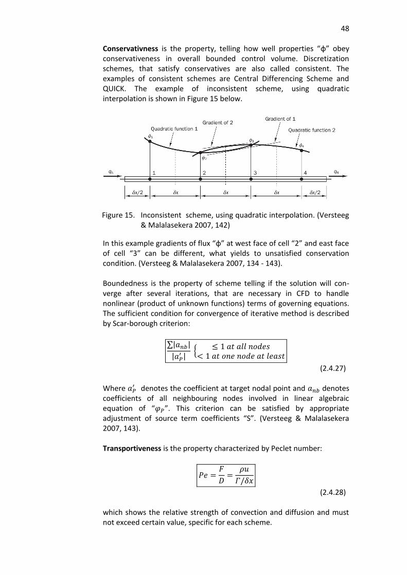
Conservativness is the property, telling how well properties “φ” obey conservativeness in overall bounded control volume. Discretization schemes, that satisfy conservatives are also called consistent. The examples of consistent schemes are Central Differencing Scheme and QUICK. The example of inconsistent scheme, using quadratic interpolation is shown in Figure 15 below.

Figure 15. Inconsistent scheme, using quadratic interpolation. (Versteeg & Malalasekera 2007, 142)

In this example gradients of flux “φ” at west face of cell “2” and east face of cell “3” can be different, what yields to unsatisfied conservation condition. (Versteeg & Malalasekera 2007, 134 - 143). Boundedness is the property of scheme telling if the solution will con-verge after several iterations, that are necessary in CFD to handle nonlinear (product of unknown functions) terms of governing equations. The sufficient condition for convergence of iterative method is described by Scar-borough criterion:

∑|𝑎𝑛𝑏|

|𝑎𝑃′ |

{≤ 1 𝑎𝑡 𝑎𝑙𝑙 𝑛𝑜𝑑𝑒𝑠

< 1 𝑎𝑡 𝑜𝑛𝑒 𝑛𝑜𝑑𝑒 𝑎𝑡 𝑙𝑒𝑎𝑠𝑡

(2.4.27) Where 𝑎𝑃

′ denotes the coefficient at target nodal point and 𝑎𝑛𝑏 denotes coefficients of all neighbouring nodes involved in linear algebraic equation of “𝜑𝑃”. This criterion can be satisfied by appropriate adjustment of source term coefficients “S”. (Versteeg & Malalasekera 2007, 143). Transportiveness is the property characterized by Peclet number:

𝑃𝑒 =𝐹

𝐷=

𝜌𝑢

𝛤/𝛿𝑥

(2.4.28) which shows the relative strength of convection and diffusion and must not exceed certain value, specific for each scheme.

49

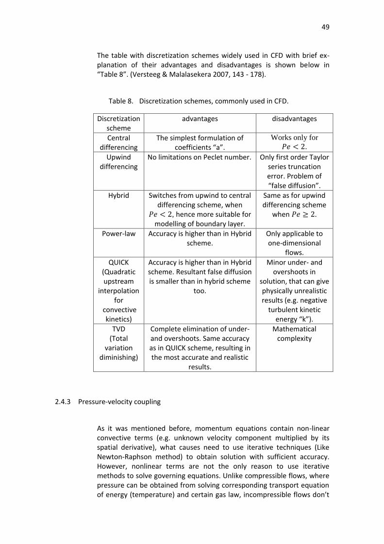
The table with discretization schemes widely used in CFD with brief ex-planation of their advantages and disadvantages is shown below in “Table 8”. (Versteeg & Malalasekera 2007, 143 - 178).

Table 8. Discretization schemes, commonly used in CFD.

Discretization scheme

advantages disadvantages

Central differencing

The simplest formulation of coefficients “a”.

Works only for

𝑃𝑒 < 2.

Upwind differencing

No limitations on Peclet number. Only first order Taylor series truncation error. Problem of “false diffusion”.

Hybrid Switches from upwind to central differencing scheme, when

𝑃𝑒 < 2, hence more suitable for modelling of boundary layer.

Same as for upwind differencing scheme

when 𝑃𝑒 ≥ 2.

Power-law Accuracy is higher than in Hybrid scheme.

Only applicable to one-dimensional

flows.

QUICK (Quadratic upstream

interpolation for

convective kinetics)

Accuracy is higher than in Hybrid scheme. Resultant false diffusion is smaller than in hybrid scheme

too.

Minor under- and overshoots in

solution, that can give physically unrealistic results (e.g. negative

turbulent kinetic energy “k”).

TVD (Total

variation diminishing)

Complete elimination of under- and overshoots. Same accuracy as in QUICK scheme, resulting in the most accurate and realistic

results.

Mathematical complexity

2.4.3 Pressure-velocity coupling

As it was mentioned before, momentum equations contain non-linear convective terms (e.g. unknown velocity component multiplied by its spatial derivative), what causes need to use iterative techniques (Like Newton-Raphson method) to obtain solution with sufficient accuracy. However, nonlinear terms are not the only reason to use iterative methods to solve governing equations. Unlike compressible flows, where pressure can be obtained from solving corresponding transport equation of energy (temperature) and certain gas law, incompressible flows don’t

50

have such relation with density and temperature, but application of correct pressure field function must yield to satisfied continuity. Therefore, one can find correct pressure function iteratively from initially guessed function, by performing certain amount of iterations, correcting the “guessed” pressure function, until continuity equations turns out to be sufficiently satisfied (converge). (Versteeg & Malalasekera 2007, 179 - 196). In order to couple the pressure and velocity to convection-diffusion equation, one has to discretize the pressure, first. There exist several methods to accomplish this problem, however only one way, called staggered grid arrangement, allows to obtain sufficiently realistic results. The pressure gradients from 2.2.25 in staggered arrangement are defined as follows:

𝜕𝑝

𝜕𝑥=

𝑝𝑃 − 𝑝𝑊

𝛿𝑥𝑊𝑃

𝜕𝑝

𝜕𝑦=

𝑝𝑃 − 𝑝𝑆

𝛿𝑦𝑆𝑃

𝜕𝑝

𝜕𝑧=

𝑝𝑃 − 𝑝𝐵

𝛿𝑧𝐵𝑃

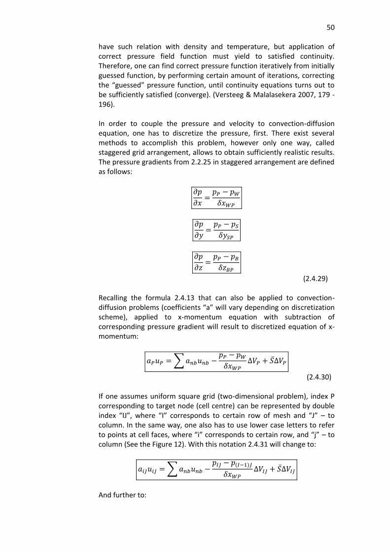
(2.4.29) Recalling the formula 2.4.13 that can also be applied to convection-diffusion problems (coefficients “a” will vary depending on discretization scheme), applied to x-momentum equation with subtraction of corresponding pressure gradient will result to discretized equation of x-momentum:

𝑎𝑃𝑢𝑃 = ∑𝑎𝑛𝑏𝑢𝑛𝑏 −𝑝𝑃 − 𝑝𝑊

𝛿𝑥𝑊𝑃∆𝑉𝑃 + 𝑆∆𝑉𝑃

(2.4.30) If one assumes uniform square grid (two-dimensional problem), index P corresponding to target node (cell centre) can be represented by double index “IJ”, where “I” corresponds to certain row of mesh and “J” – to column. In the same way, one also has to use lower case letters to refer to points at cell faces, where “i” corresponds to certain row, and “j” – to column (See the Figure 12). With this notation 2.4.31 will change to:

𝑎𝑖𝐽𝑢𝑖𝐽 = ∑𝑎𝑛𝑏𝑢𝑛𝑏 −𝑝𝐼𝐽 − 𝑝(𝐼−1)𝐽

𝛿𝑥𝑊𝑃∆𝑉𝐼𝐽 + 𝑆∆𝑉𝐼𝐽

And further to:

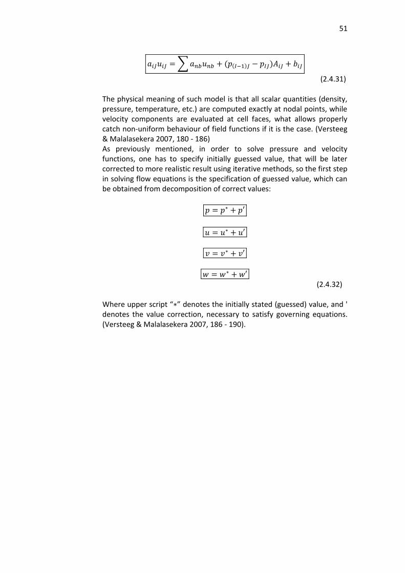
51

𝑎𝑖𝐽𝑢𝑖𝐽 = ∑𝑎𝑛𝑏𝑢𝑛𝑏 + (𝑝(𝐼−1)𝐽 − 𝑝𝐼𝐽)𝐴𝑖𝐽 + 𝑏𝑖𝐽

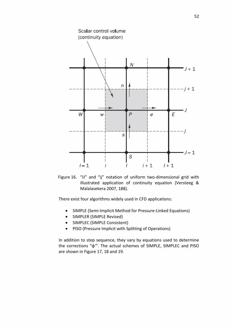
(2.4.31) The physical meaning of such model is that all scalar quantities (density, pressure, temperature, etc.) are computed exactly at nodal points, while velocity components are evaluated at cell faces, what allows properly catch non-uniform behaviour of field functions if it is the case. (Versteeg & Malalasekera 2007, 180 - 186) As previously mentioned, in order to solve pressure and velocity functions, one has to specify initially guessed value, that will be later corrected to more realistic result using iterative methods, so the first step in solving flow equations is the specification of guessed value, which can be obtained from decomposition of correct values:

𝑝 = 𝑝∗ + 𝑝′

𝑢 = 𝑢∗ + 𝑢′

𝑣 = 𝑣∗ + 𝑣′

𝑤 = 𝑤∗ + 𝑤′

(2.4.32) Where upper script “∗” denotes the initially stated (guessed) value, and ' denotes the value correction, necessary to satisfy governing equations. (Versteeg & Malalasekera 2007, 186 - 190).

52

Figure 16. “IJ” and “ij” notation of uniform two-dimensional grid with illustrated application of continuity equation (Versteeg & Malalasekera 2007, 188).

There exist four algorithms widely used in CFD applications:

SIMPLE (Semi-Implicit Method for Pressure-Linked Equations)

SIMPLER (SIMPLE Revised)

SIMPLEC (SIMPLE Consistent)

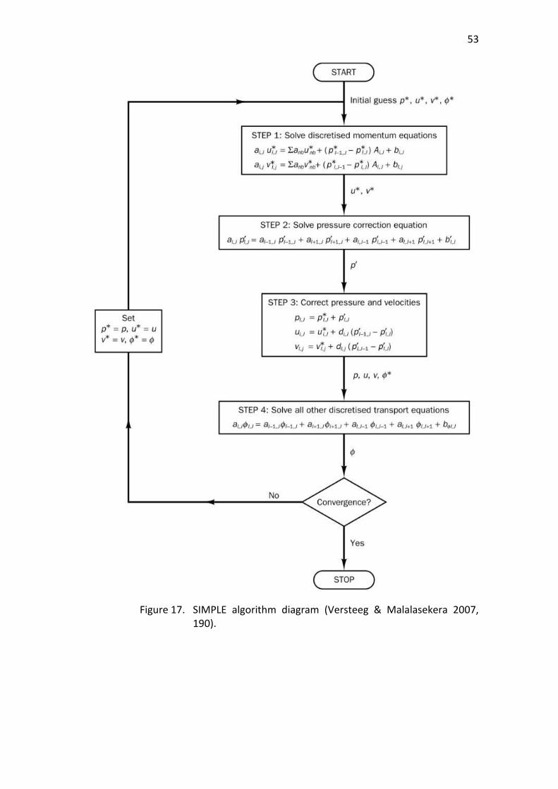
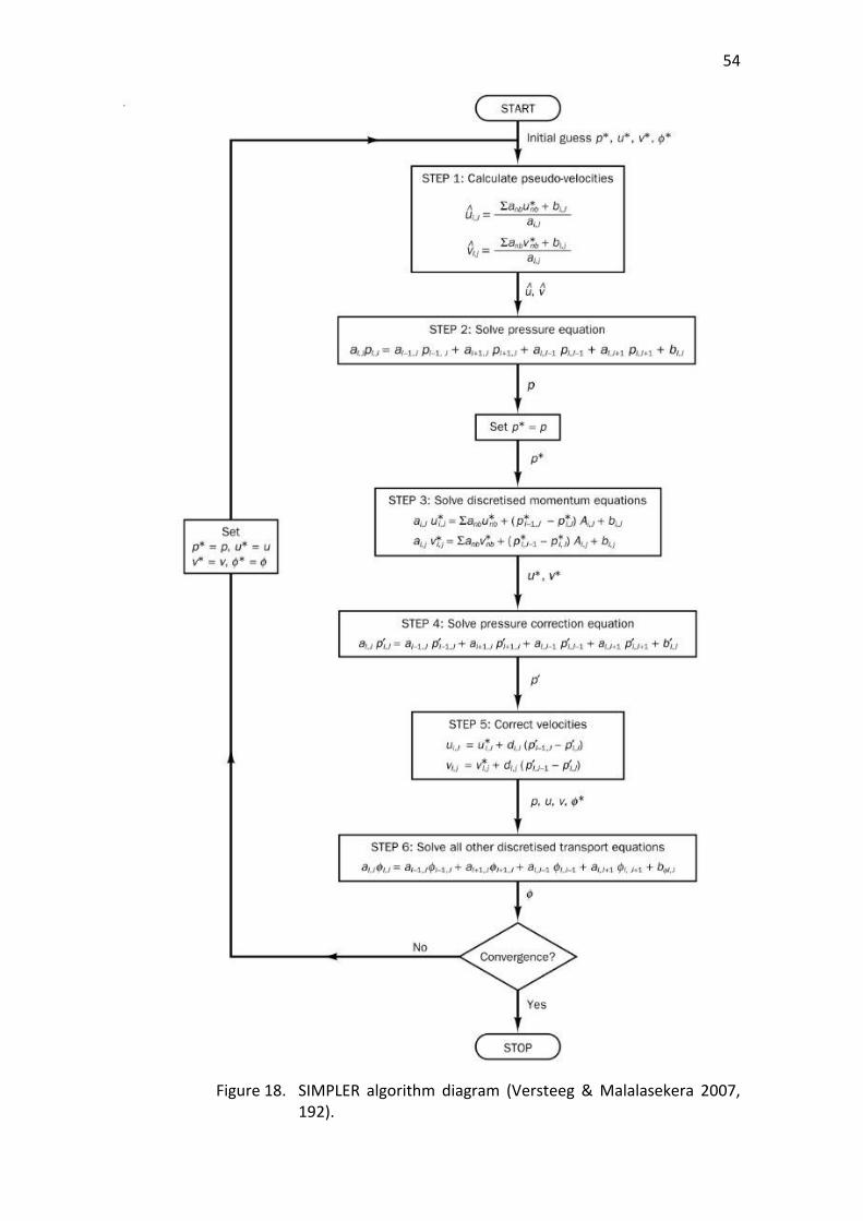
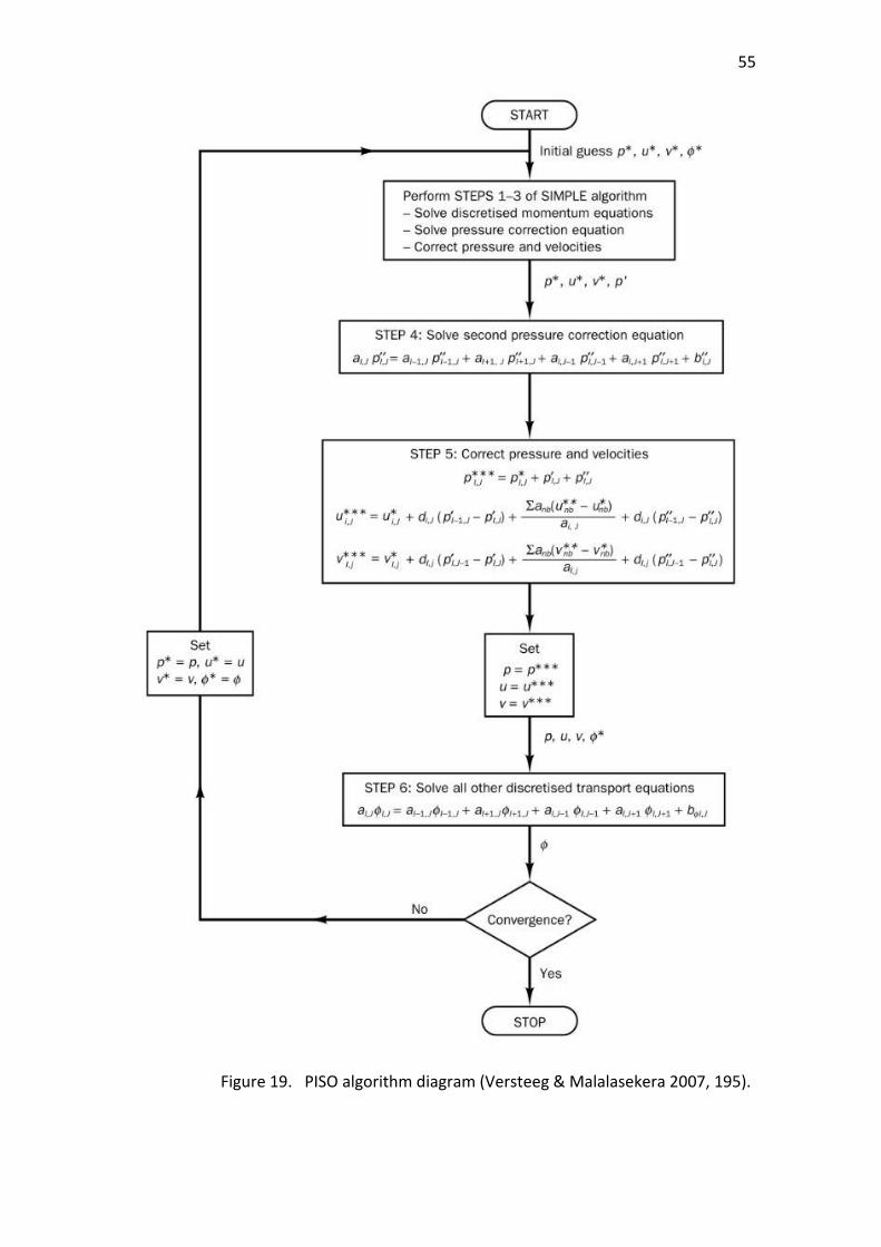
PISO (Pressure Implicit with Splitting of Operations) In addition to step sequence, they vary by equations used to determine the corrections “φ'”. The actual schemes of SIMPLE, SIMPLEC and PISO are shown in Figure 17, 18 and 19.

53

Figure 17. SIMPLE algorithm diagram (Versteeg & Malalasekera 2007, 190).

54

Figure 18. SIMPLER algorithm diagram (Versteeg & Malalasekera 2007, 192).

55

Figure 19. PISO algorithm diagram (Versteeg & Malalasekera 2007, 195).

56

Where upper script “∗∗” denotes corrected pressure, “''” denotes second correction and “∗∗∗” denotes twice-corrected pressure:

𝑝∗∗∗ = 𝑝∗∗ + 𝑝′′ = 𝑝∗ + 𝑝′ + 𝑝′′

(2.4.33) And for “𝑑” with corresponding indices:

𝑑 =𝐴

𝑎

(2.4.34) Every listed algorithm has own advantages and disadvantages. Particularly SIMPLE algorithm executes the least amount of computations per iteration, but requires more iterations to converge, while SIMPLER algorithm shows opposite behaviour due to better pressure correction scheme. On the other hand PISO shows better performance when there is no coupling of momentum equations with scalar variables (incompressible flows modelled using LES or DNS, laminar flows), while SIMPLER and SIMPLEC show better performance with highly coupled flows (compressible flows with RANS models). (Versteeg & Malalasekera 2007, 196).

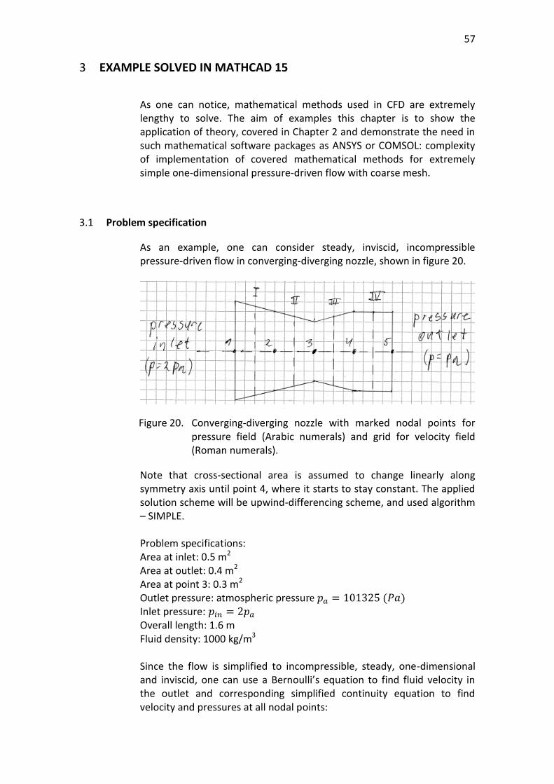
57

3 EXAMPLE SOLVED IN MATHCAD 15

As one can notice, mathematical methods used in CFD are extremely lengthy to solve. The aim of examples this chapter is to show the application of theory, covered in Chapter 2 and demonstrate the need in such mathematical software packages as ANSYS or COMSOL: complexity of implementation of covered mathematical methods for extremely simple one-dimensional pressure-driven flow with coarse mesh.

3.1 Problem specification

As an example, one can consider steady, inviscid, incompressible pressure-driven flow in converging-diverging nozzle, shown in figure 20.

Figure 20. Converging-diverging nozzle with marked nodal points for pressure field (Arabic numerals) and grid for velocity field (Roman numerals).

Note that cross-sectional area is assumed to change linearly along symmetry axis until point 4, where it starts to stay constant. The applied solution scheme will be upwind-differencing scheme, and used algorithm – SIMPLE. Problem specifications: Area at inlet: 0.5 m2 Area at outlet: 0.4 m2 Area at point 3: 0.3 m2 Outlet pressure: atmospheric pressure 𝑝𝑎 = 101325 (𝑃𝑎)

Inlet pressure: 𝑝𝑖𝑛 = 2𝑝𝑎

Overall length: 1.6 m Fluid density: 1000 kg/m3 Since the flow is simplified to incompressible, steady, one-dimensional and inviscid, one can use a Bernoulli’s equation to find fluid velocity in the outlet and corresponding simplified continuity equation to find velocity and pressures at all nodal points:

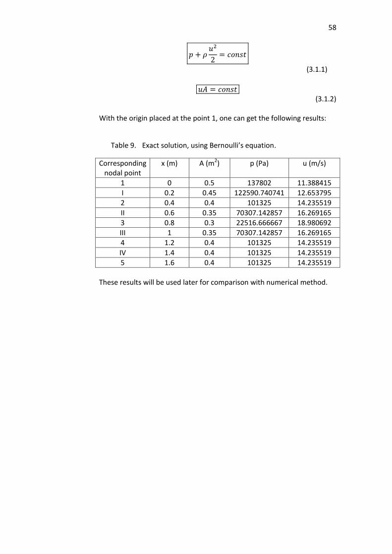
58

𝑝 + 𝜌𝑢2

2= 𝑐𝑜𝑛𝑠𝑡

(3.1.1)

𝑢𝐴 = 𝑐𝑜𝑛𝑠𝑡

(3.1.2) With the origin placed at the point 1, one can get the following results:

Table 9. Exact solution, using Bernoulli’s equation.

Corresponding nodal point

x (m) A (m2) p (Pa) u (m/s)

1 0 0.5 137802 11.388415

I 0.2 0.45 122590.740741 12.653795

2 0.4 0.4 101325 14.235519

II 0.6 0.35 70307.142857 16.269165

3 0.8 0.3 22516.666667 18.980692

III 1 0.35 70307.142857 16.269165

4 1.2 0.4 101325 14.235519

IV 1.4 0.4 101325 14.235519

5 1.6 0.4 101325 14.235519

These results will be used later for comparison with numerical method.

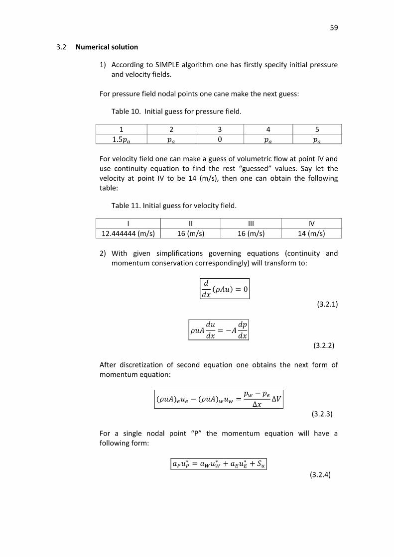
59

3.2 Numerical solution

1) According to SIMPLE algorithm one has firstly specify initial pressure and velocity fields.

For pressure field nodal points one cane make the next guess:

Table 10. Initial guess for pressure field.

1 2 3 4 5

1.5𝑝𝑎 𝑝𝑎 0 𝑝𝑎 𝑝𝑎

For velocity field one can make a guess of volumetric flow at point IV and use continuity equation to find the rest “guessed” values. Say let the velocity at point IV to be 14 (m/s), then one can obtain the following table:

Table 11. Initial guess for velocity field.

I II III IV

12.444444 (m/s) 16 (m/s) 16 (m/s) 14 (m/s)

2) With given simplifications governing equations (continuity and

momentum conservation correspondingly) will transform to:

𝑑

𝑑𝑥(𝜌𝐴𝑢) = 0

(3.2.1)

𝜌𝑢𝐴𝑑𝑢

𝑑𝑥= −𝐴

𝑑𝑝

𝑑𝑥

(3.2.2) After discretization of second equation one obtains the next form of momentum equation:

(𝜌𝑢𝐴)𝑒𝑢𝑒 − (𝜌𝑢𝐴)𝑤𝑢𝑤 =𝑝𝑤 − 𝑝𝑒

∆𝑥∆𝑉

(3.2.3) For a single nodal point “P” the momentum equation will have a following form:

𝑎𝑃𝑢𝑃∗ = 𝑎𝑊𝑢𝑊

∗ + 𝑎𝐸𝑢𝐸∗ + 𝑆𝑢

(3.2.4)

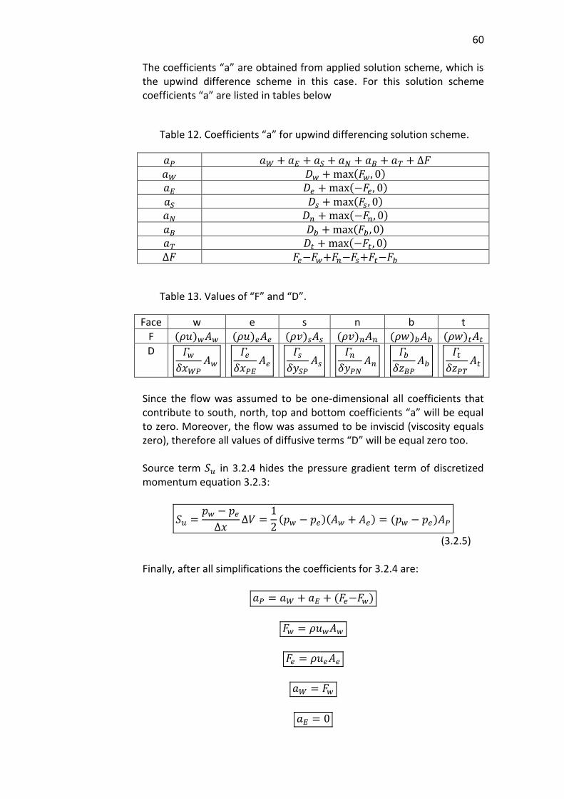
60

The coefficients “a” are obtained from applied solution scheme, which is the upwind difference scheme in this case. For this solution scheme coefficients “a” are listed in tables below

Table 12. Coefficients “a” for upwind differencing solution scheme.

𝑎𝑃 𝑎𝑊 + 𝑎𝐸 + 𝑎𝑆 + 𝑎𝑁 + 𝑎𝐵 + 𝑎𝑇 + ∆𝐹

𝑎𝑊 𝐷𝑤 + max(𝐹𝑤, 0)

𝑎𝐸 𝐷𝑒 + max(−𝐹𝑒 , 0)

𝑎𝑆 𝐷𝑠 + max(𝐹𝑠, 0)

𝑎𝑁 𝐷𝑛 + max(−𝐹𝑛, 0)

𝑎𝐵 𝐷𝑏 + max(𝐹𝑏 , 0)

𝑎𝑇 𝐷𝑡 + max(−𝐹𝑡, 0)

∆𝐹 𝐹𝑒−𝐹𝑤+𝐹𝑛−𝐹𝑠+𝐹𝑡−𝐹𝑏

Table 13. Values of “F” and “D”.

Face w e s n b t

F (𝜌𝑢)𝑤𝐴𝑤 (𝜌𝑢)𝑒𝐴𝑒 (𝜌𝑣)𝑠𝐴𝑠 (𝜌𝑣)𝑛𝐴𝑛 (𝜌𝑤)𝑏𝐴𝑏 (𝜌𝑤)𝑡𝐴𝑡

D 𝛤𝑤

𝛿𝑥𝑊𝑃𝐴𝑤

𝛤𝑒

𝛿𝑥𝑃𝐸𝐴𝑒

𝛤𝑠

𝛿𝑦𝑆𝑃𝐴𝑠

𝛤𝑛

𝛿𝑦𝑃𝑁𝐴𝑛

𝛤𝑏

𝛿𝑧𝐵𝑃𝐴𝑏

𝛤𝑡

𝛿𝑧𝑃𝑇𝐴𝑡

Since the flow was assumed to be one-dimensional all coefficients that contribute to south, north, top and bottom coefficients “a” will be equal to zero. Moreover, the flow was assumed to be inviscid (viscosity equals zero), therefore all values of diffusive terms “D” will be equal zero too. Source term 𝑆𝑢 in 3.2.4 hides the pressure gradient term of discretized momentum equation 3.2.3:

𝑆𝑢 =𝑝𝑤 − 𝑝𝑒

∆𝑥∆𝑉 =

1

2(𝑝𝑤 − 𝑝𝑒)(𝐴𝑤 + 𝐴𝑒) = (𝑝𝑤 − 𝑝𝑒)𝐴𝑃

(3.2.5) Finally, after all simplifications the coefficients for 3.2.4 are:

𝑎𝑃 = 𝑎𝑊 + 𝑎𝐸 + (𝐹𝑒−𝐹𝑤)

𝐹𝑤 = 𝜌𝑢𝑤𝐴𝑤

𝐹𝑒 = 𝜌𝑢𝑒𝐴𝑒

𝑎𝑊 = 𝐹𝑤

𝑎𝐸 = 0

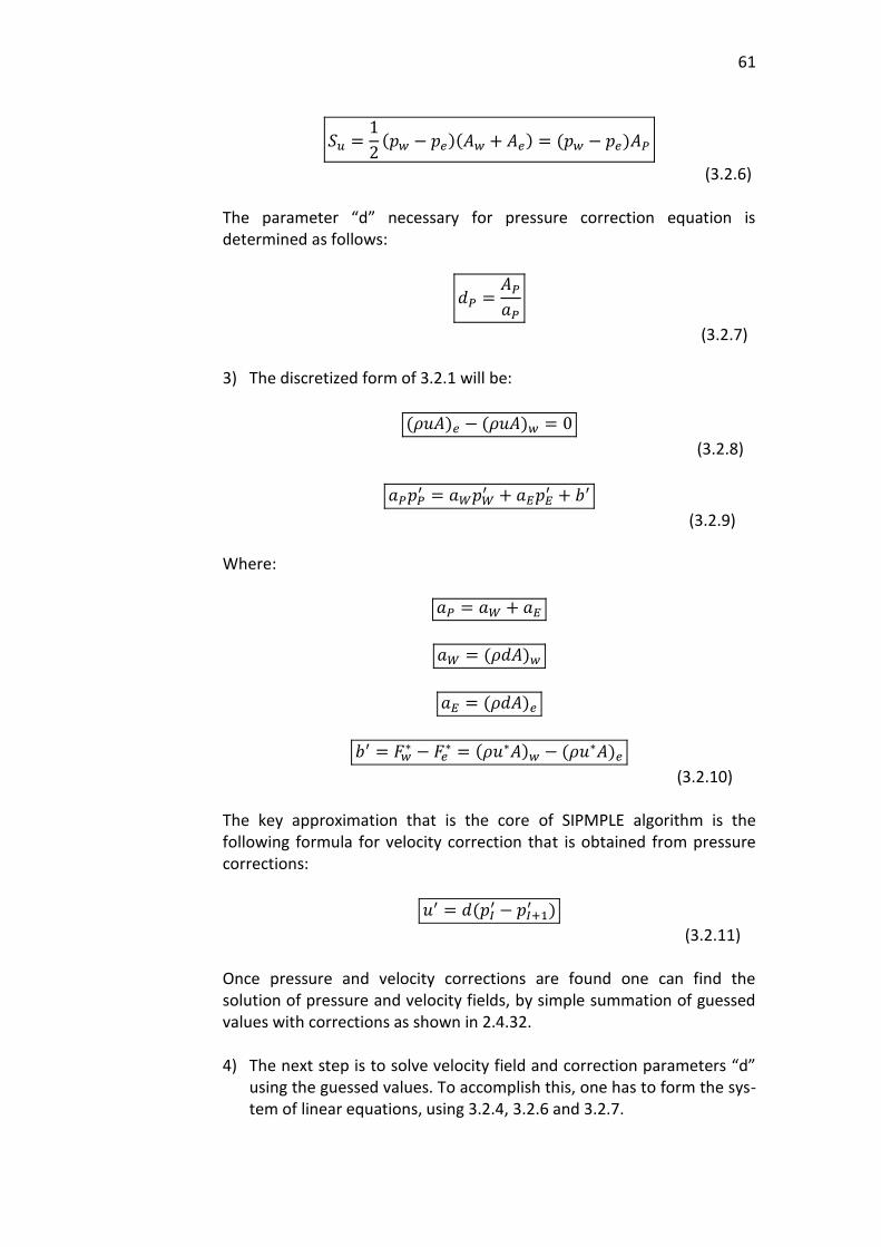
61

𝑆𝑢 =1

2(𝑝𝑤 − 𝑝𝑒)(𝐴𝑤 + 𝐴𝑒) = (𝑝𝑤 − 𝑝𝑒)𝐴𝑃

(3.2.6) The parameter “d” necessary for pressure correction equation is determined as follows:

𝑑𝑃 =𝐴𝑃

𝑎𝑃

(3.2.7) 3) The discretized form of 3.2.1 will be:

(𝜌𝑢𝐴)𝑒 − (𝜌𝑢𝐴)𝑤 = 0

(3.2.8)

𝑎𝑃𝑝𝑃′ = 𝑎𝑊𝑝𝑊

′ + 𝑎𝐸𝑝𝐸′ + 𝑏′

(3.2.9) Where:

𝑎𝑃 = 𝑎𝑊 + 𝑎𝐸

𝑎𝑊 = (𝜌𝑑𝐴)𝑤

𝑎𝐸 = (𝜌𝑑𝐴)𝑒

𝑏′ = 𝐹𝑤∗ − 𝐹𝑒

∗ = (𝜌𝑢∗𝐴)𝑤 − (𝜌𝑢∗𝐴)𝑒

(3.2.10) The key approximation that is the core of SIPMPLE algorithm is the following formula for velocity correction that is obtained from pressure corrections:

𝑢′ = 𝑑(𝑝𝐼′ − 𝑝𝐼+1

′ )

(3.2.11) Once pressure and velocity corrections are found one can find the solution of pressure and velocity fields, by simple summation of guessed values with corrections as shown in 2.4.32. 4) The next step is to solve velocity field and correction parameters “d”

using the guessed values. To accomplish this, one has to form the sys-tem of linear equations, using 3.2.4, 3.2.6 and 3.2.7.

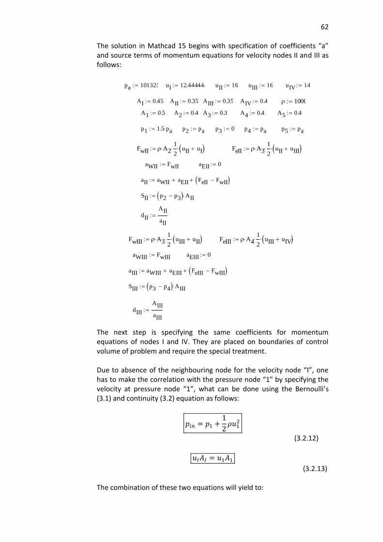
62

The solution in Mathcad 15 begins with specification of coefficients “a” and source terms of momentum equations for velocity nodes II and III as follows:

The next step is specifying the same coefficients for momentum equations of nodes I and IV. They are placed on boundaries of control volume of problem and require the special treatment. Due to absence of the neighbouring node for the velocity node “I”, one has to make the correlation with the pressure node “1” by specifying the velocity at pressure node “1”, what can be done using the Bernoulli’s (3.1) and continuity (3.2) equation as follows:

𝑝𝑖𝑛 = 𝑝1 +1

2𝜌𝑢1

2

(3.2.12)

𝑢𝐼𝐴𝐼 = 𝑢1𝐴1

(3.2.13) The combination of these two equations will yield to:

pa 101325 uI 12.444444 uII 16 uIII 16 uIV 14

AI 0.45 AII 0.35 AIII 0.35 AIV 0.4 1000

A1 0.5 A2 0.4 A3 0.3 A4 0.4 A5 0.4

p1 1.5 pa p2 pa p3 0 p4 pa p5 pa

FwII A21

2 uII uI FeII A3

1

2 uII uIII

aWII FwII aEII 0

aII aWII aEII FeII FwII

SII p2 p3 AII

dII

AII

aII

FwIII A31

2 uIII uII FeIII A4

1

2 uIII uIV

aWIII FwIII aEIII 0

aIII aWIII aEIII FeIII FwIII

SIII p3 p4 AIII

dIII

AIII

aIII

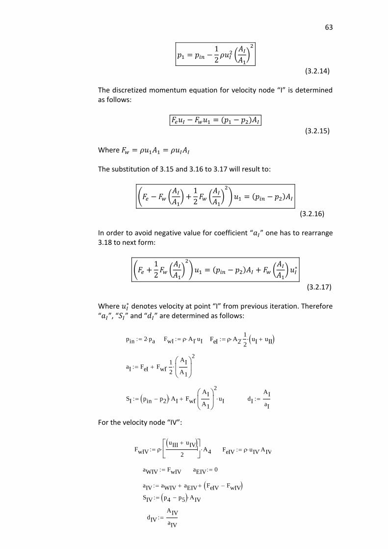
63

𝑝1 = 𝑝𝑖𝑛 −1

2𝜌𝑢𝐼

2 (𝐴𝐼

𝐴1)

2

(3.2.14) The discretized momentum equation for velocity node “I” is determined as follows:

𝐹𝑒𝑢𝐼 − 𝐹𝑤𝑢1 = (𝑝1 − 𝑝2)𝐴𝐼

(3.2.15) Where 𝐹𝑤 = 𝜌𝑢1𝐴1 = 𝜌𝑢𝐼𝐴𝐼 The substitution of 3.15 and 3.16 to 3.17 will result to:

(𝐹𝑒 − 𝐹𝑤 (𝐴𝐼

𝐴1) +

1

2𝐹𝑤 (

𝐴𝐼

𝐴1)

2

)𝑢1 = (𝑝𝑖𝑛 − 𝑝2)𝐴𝐼

(3.2.16) In order to avoid negative value for coefficient “𝑎𝐼” one has to rearrange 3.18 to next form:

(𝐹𝑒 +1

2𝐹𝑤 (

𝐴𝐼

𝐴1)

2

)𝑢1 = (𝑝𝑖𝑛 − 𝑝2)𝐴𝐼 + 𝐹𝑤 (𝐴𝐼

𝐴1) 𝑢𝐼

∗

(3.2.17) Where 𝑢𝐼

∗ denotes velocity at point “I” from previous iteration. Therefore “𝑎𝐼”, “𝑆𝐼” and “𝑑𝐼” are determined as follows:

For the velocity node “IV”:

pin 2 pa FwI AI uI FeI A21

2 uI uII

aI FeI FwI1

2

AI

A1

2

SI pin p2 AI FwI

AI

A1

2

uI dI

AI

aI

FwIV uIII uIV

2

A4 FeIV uIV AIV

aWIV FwIV aEIV 0

aIV aWIV aEIV FeIV FwIV

SIV p4 p5 AIV

dIV

AIV

aIV

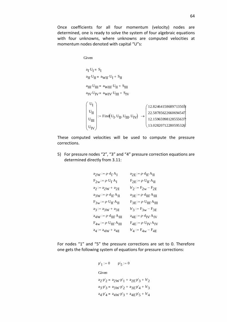
64

Once coefficients for all four momentum (velocity) nodes are determined, one is ready to solve the system of four algebraic equations with four unknowns, where unknowns are computed velocities at momentum nodes denoted with capital “U”s:

These computed velocities will be used to compute the pressure corrections. 5) For pressure nodes “2”, “3” and “4” pressure correction equations are

determined directly from 3.11: For nodes “1” and “5” the pressure corrections are set to 0. Therefore one gets the following system of equations for pressure corrections:

Given

aI UI SI

aII UII aWII UI SII

aIII UIII aWIII UII SIII

aIV UIV aWIV UIII SIV

UI

UII

UIII

UIV

Find UI UII UIII UIV

12.824641586897135038

22.587856226606945473

12.159659981285556379

13.028207122805953263

a2W dI AI a2E dII AII

F2w UI AI F2E UII AII

a2 a2W a2E b'2 F2w F2E

a3W dII AII a3E dIII AIII

F3w UII AII F3E UIII AIII


a4W dIII AIII a4E dIV AIV

F4w UIII AIII F4E UIV AIV


p'1 0 p'5 0

Given

a2 p'2 a2W p'1 a2E p'3 b'2

a3 p'3 a3W p'2 a3E p'4 b'3

a4 p'4 a4W p'3 a4E p'5 b'4

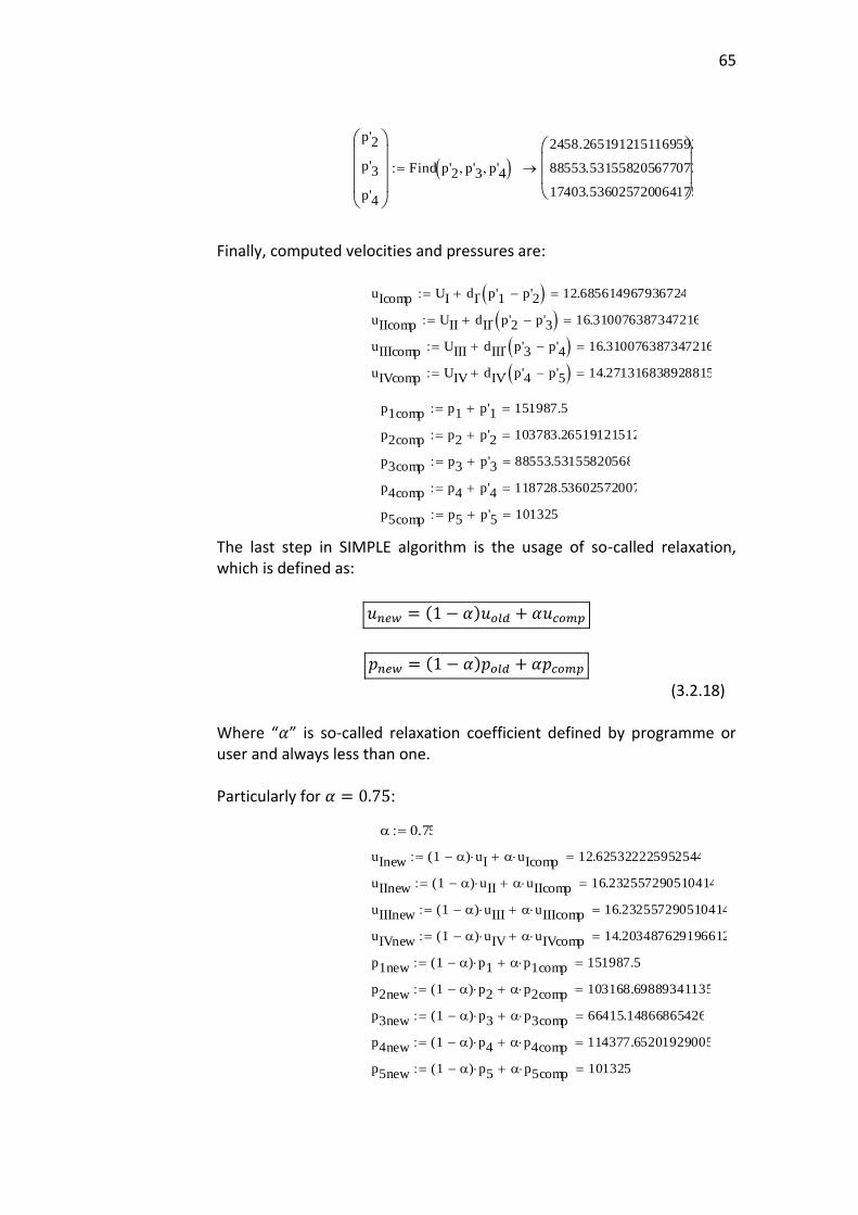
65

Finally, computed velocities and pressures are: The last step in SIMPLE algorithm is the usage of so-called relaxation, which is defined as:

𝑢𝑛𝑒𝑤 = (1 − 𝛼)𝑢𝑜𝑙𝑑 + 𝛼𝑢𝑐𝑜𝑚𝑝

𝑝𝑛𝑒𝑤 = (1 − 𝛼)𝑝𝑜𝑙𝑑 + 𝛼𝑝𝑐𝑜𝑚𝑝

(3.2.18) Where “𝛼” is so-called relaxation coefficient defined by programme or user and always less than one. Particularly for 𝛼 = 0.75:

p'2

p'3

p'4

Find p'2 p'3 p'4 2458.2651912151169592

88553.531558205677073

17403.536025720064175

uIcomp UI dI p'1 p'2 12.685614967936724

uIIcomp UII dII p'2 p'3 16.310076387347216

uIIIcomp UIII dIII p'3 p'4 16.310076387347216

uIVcomp UIV dIV p'4 p'5 14.271316838928815

p1comp p1 p'1 151987.5

p2comp p2 p'2 103783.26519121512

p3comp p3 p'3 88553.53155820568

p4comp p4 p'4 118728.53602572007

p5comp p5 p'5 101325

0.75

uInew 1 ( ) uI uIcomp 12.625322225952544

uIInew 1 ( ) uII uIIcomp 16.232557290510414

uIIInew 1 ( ) uIII uIIIcomp 16.232557290510414

uIVnew 1 ( ) uIV uIVcomp 14.203487629196612

p1new 1 ( ) p1 p1comp 151987.5

p2new 1 ( ) p2 p2comp 103168.69889341135

p3new 1 ( ) p3 p3comp 66415.14866865426

p4new 1 ( ) p4 p4comp 114377.65201929005

p5new 1 ( ) p5 p5comp 101325

66

The last set of values is the outcome of a single iteration in SIMPLE algorithm. In order to execute the second iteration one simply has to set the final result of first iteration as guess values for second iteration and repeat the procedure. Results (except pressures at nodes “1” (because in most CFD codes this value will be reserved for stagnation pressure at pressure inlet, which is double atmospheric pressure in this case must not change with any number of performed iterations) and “3”) show some agreement with the exact solution in Table 9 even though they not necessary should, since the grid consist only from five pressure a four momentum (velocity) nodes, that makes it to be a relatively coarse mesh. The accuracy can be improved by the grid refinement (increasing the amount of nodes). But one must remember that this will increase the complexity of mathematical model and require more iterations to converge (Versteeg & Malalasekera 2007, 209 -210). The disadvantage of poor accuracy in numerical methods is compensated by their ability to be expanded to more complex three-dimensional, compressible, viscous and even ionized flows, what together with the absence of alternatives ensured the popularity of CFD in industrial and scientific applications. Considered example explicitly shows how lengthy the computation of flow can be even with coarse mesh. Therefore, in order to handle more complex scenarios such as three-dimensional transient flow, it’s strongly suggested to use either commercial software like ANSYS or COMSOL or any free CFD software, that can be found here: https://www.cfd-online.com/Wiki/Codes.

In order to learn how to use ANSYS FLUENT one can go to link below which contains tutorials in FLUENT covering all aspects, necessary to know for modelling of complex flows. Link to ANSYS FLUENT tutorials: https://confluence.cornell.edu/display/SIMULATION/FLUENT+Learning+Modules

Once tutorials are completed, one can continue the self-study by exploring the following book, which also gives the insight into programming aspects of CFD: Moukalled F., Mangani L., Darwish M. (2016) The Finite Volume Method in Computational Fluid Dynamics: An Advanced Introduction with OpenFOAM and Matlab. Stuttgart: Springer.

https://www.cfd-online.com/Wiki/Codes

https://confluence.cornell.edu/display/SIMULATION/FLUENT+Learning+Modules


67

4 PI-THEOREM HANDOUTS

CFD provides Mechanical Engineering designers with an inexpensive alternative to actual experiments supported by a high flexibility in changing of prototype design. However, once the results from several simulations are obtained, one has to build up satisfactory mathematical models. The main difficulty at this stage is usually a wide range of variables involved in the simulated process including: velocity at inlet, the density and viscosity of the fluid, ambient temperature, thermal conductivity, drag force, geometry of control volume, frequency of vibration, enthalpy etc., making the question of which variables are dependent on each other to be difficult to handle. To answer this question completely, one can use the Bucking-ham Pi-Theorem (or simply Pi-Theorem). The Pi-Theorem states that any set of variables can be changed to the set of distinct non-dimensional groups, that are dependent on each other. The exact dependence is deter-mined from experimental data and curve-fitting techniques. In order to understand the process of non-dimensional Pi-groups’ formulation, one has to consider the dimension of every variable involved into experiment or simulation. The examples of dimensions are listed in Table.14.

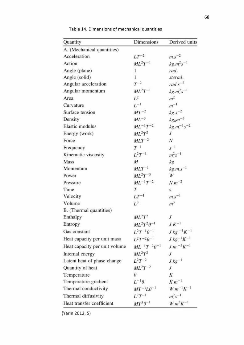
68

Table 14. Dimensions of mechanical quantities

(Yarin 2012, 5)

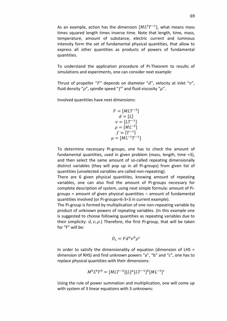
69

As an example, action has the dimension [𝑀𝐿2𝑇−1], what means mass times squared length times inverse time. Note that length, time, mass, temperature, amount of substance, electric current and luminous intensity form the set of fundamental physical quantities, that allow to express all other quantities as products of powers of fundamental quantities. To understand the application procedure of Pi-Theorem to results of simulations and experiments, one can consider next example: Thrust of propeller “𝐹” depends on diameter “𝑑”, velocity at inlet “𝑣”, fluid density “𝜌”, spindle speed “𝑓” and fluid viscosity “𝜇”. Involved quantities have next dimensions:

𝐹 = [𝑀𝐿𝑇−2] 𝑑 = [𝐿]

𝑣 = [𝐿𝑇−1] 𝜌 = [𝑀𝐿−3] 𝑓 = [𝑇−1]

𝜇 = [𝑀𝐿−1𝑇−1] To determine necessary Pi-groups, one has to check the amount of fundamental quantities, used in given problem (mass, length, time =3), and then select the same amount of so-called repeating dimensionally distinct variables (they will pop up in all Pi-groups) from given list of quantities (unselected variables are called non-repeating). There are 6 given physical quantities, knowing amount of repeating variables, one can also find the amount of Pi-groups necessary for complete description of system, using next simple formula: amount of Pi-groups = amount of given physical quantities – amount of fundamental quantities involved (or Pi-groups=6-3=3 in current example). The Pi-group is formed by multiplication of one non-repeating variable by product of unknown powers of repeating variables. (In this example one is suggested to choose following quantities as repeating variables due to their simplicity: 𝑑, 𝑣, 𝜌.) Therefore, the first Pi-group, that will be taken for “F” will be:

𝛱1 = 𝐹𝑑𝑎𝑣𝑏𝜌𝑐

In order to satisfy the dimensionality of equation (dimension of LHS = dimension of RHS) and find unknown powers “a”, “b” and “c”, one has to replace physical quantities with their dimensions:

𝑀0𝐿0𝑇0 = [𝑀𝐿𝑇−2][𝐿]𝑎[𝐿𝑇−1]𝑏[𝑀𝐿−3]𝑐

Using the rule of power summation and multiplication, one will come up with system of 3 linear equations with 3 unknowns:

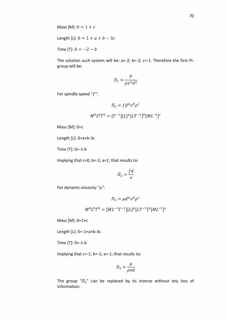
70

Mass [M]: 0 = 1 + 𝑐 Length [L]: 0 = 1 + 𝑎 + 𝑏 − 3𝑐 Time [T]: 0 = −2 − 𝑏 The solution such system will be: a=-2; b=-2; c=-1. Therefore the first Pi-group will be:

𝛱1 =𝐹

𝜌𝑣2𝑑2

For spindle speed “𝑓”:

𝛱2 = 𝑓𝑑𝑎𝑣𝑏𝜌𝑐

𝑀0𝐿0𝑇0 = [𝑇−1][𝐿]𝑎[𝐿𝑇−1]𝑏[𝑀𝐿−3]𝑐

Mass [M]: 0=c Length [L]: 0=a+b-3c Time [T]: 0=-1-b Implying that c=0; b=-1; a=1; that results to:

𝛱2 =𝑓𝑑

𝑣

For dynamic viscosity “𝜇”:

𝛱3 = 𝜇𝑑𝑎𝑣𝑏𝜌𝑐

𝑀0𝐿0𝑇0 = [𝑀𝐿−1𝑇−1][𝐿]𝑎[𝐿𝑇−1]𝑏[𝑀𝐿−3]𝑐

Mass [M]: 0=1+c Length [L]: 0=-1+a+b-3c Time [T]: 0=-1-b Implying that c=-1; b=-1; a=-1; that results to:

𝛱3 =𝜇

𝜌𝑣𝑑

The group “𝛱3” can be replaced by its inverse without any loss of information:

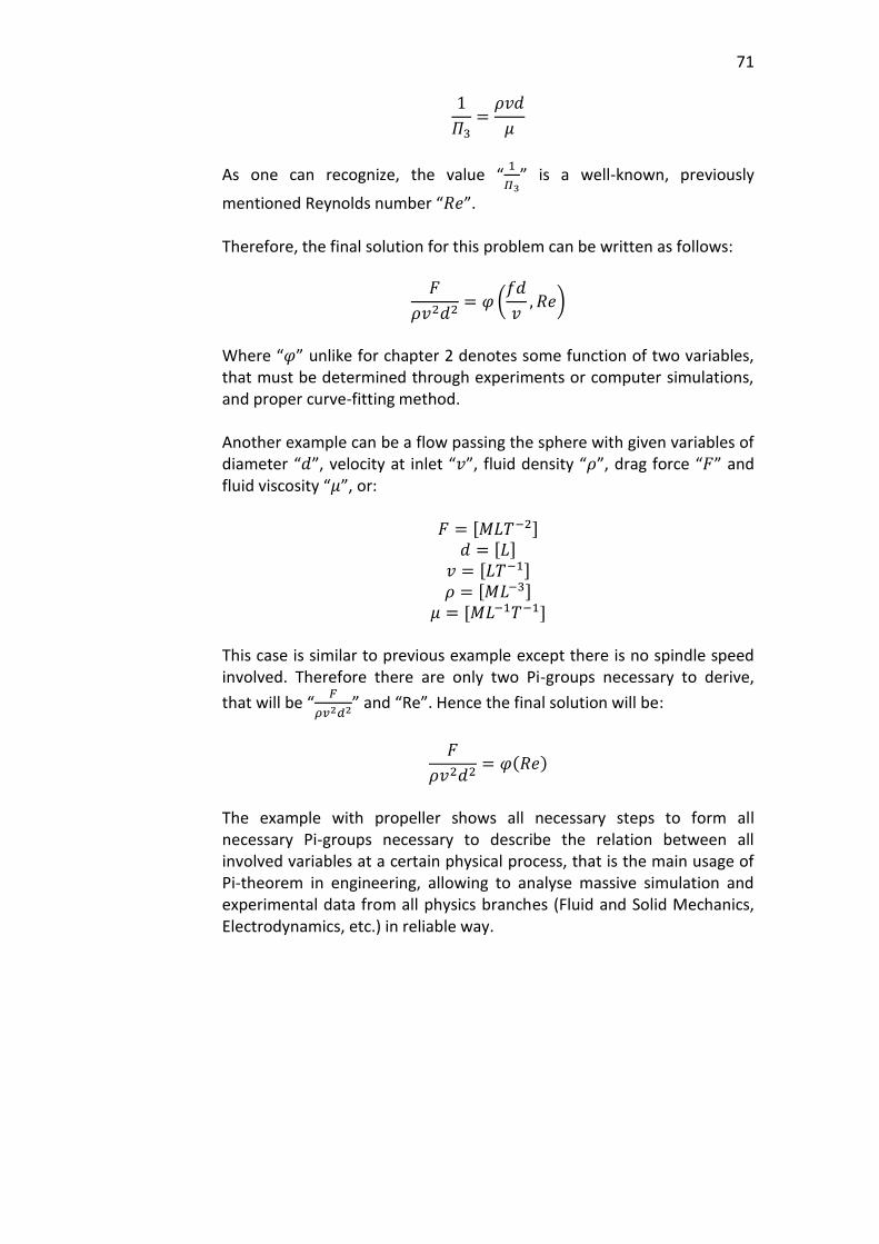
71

1

𝛱3=

𝜌𝑣𝑑

𝜇

As one can recognize, the value “1

𝛱3” is a well-known, previously

mentioned Reynolds number “𝑅𝑒”. Therefore, the final solution for this problem can be written as follows:

𝐹

𝜌𝑣2𝑑2= 𝜑 (

𝑓𝑑

𝑣, 𝑅𝑒)

Where “𝜑” unlike for chapter 2 denotes some function of two variables, that must be determined through experiments or computer simulations, and proper curve-fitting method. Another example can be a flow passing the sphere with given variables of diameter “𝑑”, velocity at inlet “𝑣”, fluid density “𝜌”, drag force “𝐹” and fluid viscosity “𝜇”, or:

𝐹 = [𝑀𝐿𝑇−2] 𝑑 = [𝐿]

𝑣 = [𝐿𝑇−1] 𝜌 = [𝑀𝐿−3]

𝜇 = [𝑀𝐿−1𝑇−1] This case is similar to previous example except there is no spindle speed involved. Therefore there are only two Pi-groups necessary to derive,

that will be “𝐹

𝜌𝑣2𝑑2” and “Re”. Hence the final solution will be:

𝐹

𝜌𝑣2𝑑2= 𝜑(𝑅𝑒)

The example with propeller shows all necessary steps to form all necessary Pi-groups necessary to describe the relation between all involved variables at a certain physical process, that is the main usage of Pi-theorem in engineering, allowing to analyse massive simulation and experimental data from all physics branches (Fluid and Solid Mechanics, Electrodynamics, etc.) in reliable way.

72

5 CONCLUSION.

The material listed in this work is a sufficient minimum for students, who are just starting to explore the capabilities of computational Physics, necessary to understand, what will happen inside such solvers as FLUENT once the tutorial completing has begun and to properly justify the correct-ness of obtained results. Included FLUENT Tutorials from Cornell University on the other hand provide new students with necessary experience in application of CFD to real engineering problems. A literature for further reading after finishing of tutorials was also suggested.

73

REFERENCES

Moukalled F., Mangani L., Darwish M. (2016) The Finite Volume Method in Computational Fluid Dynamics: An Advanced Introduction with Open-FOAM and Matlab. Stuttgart: Springer. Schlichting H. (1979) Boundary-layer Theory. New-York: McGraw-Hill Versteeg H. K. & W. Malalasekera. (2007) An Introduction to Computational Fluid Dynamics: The Finite Volume Method. Harlow: Pearson Education Limited. Yarin L.P. (2012) The Pi-Theorem, Applications to Fluid Mechanics and Heat and Mass Transfer. Berlin: Springer. CFD-online (n.d.). Retrieved 5 May 2017 https://www.cfd-online.com/ computationalfluiddynamics.com.au (n.d.). Retrieved 5 May 2017 https://www.computationalfluiddynamics.com.au Experiment with an ink in a water flow (n.d.). Retrieved 5 May 2017 from http://www.azimuthproject.org/azimuth/show/Blog+-+eddy+who%3F FLUENT tutorials from Cornell University (n.d). Retrieved 5 May 2017 https://confluence.cornell.edu/display/SIMULATION/FLUENT+Learning+Modules Laminar flow past sphere (n.d.). Retrieved 5 May 2017. https://user.engineering.uiowa.edu/~cfd/gallery/lim-turb.html Tracking the path of a single fluid particle, done with Lagrange approach (n.d.). Retrieved 5 May 2017 http://hoskere2.web.engr.illinois.edu/cs445/finalProject/ Turbulent flow past sphere (n.d.). Retrieved 5 May 2017. https://user.engineering.uiowa.edu/~cfd/gallery/lim-turb.html Visualization of flow as function of time and space done in Eularian approach (n.d.). Retrieved 5 May 2017 http://hoskere2.web.engr.illinois.edu/cs445/finalProject/

https://www.cfd-online.com/

https://www.computationalfluiddynamics.com.au/

http://www.azimuthproject.org/azimuth/show/Blog+-+eddy+who%3F



https://user.engineering.uiowa.edu/~cfd/gallery/lim-turb.html

http://hoskere2.web.engr.illinois.edu/cs445/finalProject/

https://user.engineering.uiowa.edu/~cfd/gallery/lim-turb.html

http://hoskere2.web.engr.illinois.edu/cs445/finalProject/

74

Wall functions are not applicable to problems involving a flow separation (2012). Retrieved 5 May 2017. https://www.computationalfluiddynamics.com.au/tips-tricks-turbulence-wall-functions-and-y-requirements/ www.quora.com (2015). Retrieved 5 May 2017 https://www.quora.com/What-is-the-difference-between-lagrangian-and-Eulerian-approach

https://www.computationalfluiddynamics.com.au/tips-tricks-turbulence-wall-functions-and-y-requirements/

https://www.computationalfluiddynamics.com.au/tips-tricks-turbulence-wall-functions-and-y-requirements/

https://www.quora.com/What-is-the-difference-between-lagrangian-and-Eulerian-approach

https://www.quora.com/What-is-the-difference-between-lagrangian-and-Eulerian-approach

75

Documents

Self-study manual for introduction to computational fluid