Embed Size (px)
Citation preview

This article has been accepted for publication and undergone full peer review but has not been through the copyediting, typesetting, pagination and proofreading process which may lead to differences between this version and the Version of Record. Please cite this article as doi: 10.1029/2019JA026475
© 2019 American Geophysical Union. All rights reserved.
Good Simon W. (Orcid ID: 0000-0002-4921-4208)
Kilpua Emilia (Orcid ID: 0000-0002-4489-8073)
LaMoury Adrian T. (Orcid ID: 0000-0003-1551-5325)
Forsyth Robert J (Orcid ID: 0000-0003-2701-0375)
Eastwood Jonathan P. (Orcid ID: 0000-0003-4733-8319)
Möstl Christian (Orcid ID: 0000-0001-6868-4152)
Self-Similarity of ICME Flux Ropes: Observations by Radially Aligned
Spacecraft in the Inner Heliosphere
S. W. Good1, E. K. J. Kilpua
1, A. T. LaMoury
2, R. J. Forsyth
2, J. P. Eastwood
2, and
C. Möstl3
1Department of Physics, University of Helsinki, Helsinki, Finland
2The Blackett Laboratory, Imperial College London, London, UK
3Space Research Institute, Austrian Academy of Sciences, Graz, Austria
Corresponding author: Simon Good ([email protected])
Key Points:
● Eighteen interplanetary flux ropes observed by radially aligned spacecraft in the inner
heliosphere have been examined
● Many of the flux ropes showed significant self-similarities in magnetic field structure
at the aligned spacecraft
● Macroscale differences in the magnetic field profiles are consistent with the flux ropes
displaying different axis orientations

© 2019 American Geophysical Union. All rights reserved.
Abstract
Interplanetary coronal mass ejections (ICMEs) are a significant feature of the heliospheric
environment and the primary cause of adverse space weather at the Earth. ICME
propagation, and the evolution of ICME magnetic field structure during propagation, are still
not fully understood. We analyze the magnetic field structures of 18 ICME magnetic flux
ropes observed by radially aligned spacecraft in the inner heliosphere. Similarity in the
underlying flux rope structures is determined through the application of a simple technique
that maps the magnetic field profile from one spacecraft to the other. In many cases, the flux
ropes show very strong underlying similarities at the different spacecraft. The mapping
technique reveals similarities that are not readily apparent in the unmapped data and is a
useful tool when determining whether magnetic field time series observed at different
spacecraft are associated with the same ICME. Lundquist fitting has been applied to the flux
ropes and the rope orientations have been determined; macroscale differences in the profiles
at the aligned spacecraft may be ascribed to differences in flux rope orientation. Assuming
that the same region of the ICME was observed by the aligned spacecraft in each case, the
fitting indicates some weak tendency for the rope axes to reduce in inclination relative to the
solar equatorial plane and to align with the solar east-west direction with heliocentric
distance.
Plain Language Summary
Coronal mass ejections (CMEs) are large eruptions of magnetic field and plasma from the
Sun. When they arrive at the Earth, these eruptions can cause significant damage to ground
and orbital infrastructure; forecasting this ‘space weather’ impact of CMEs at the Earth
remains a difficult task. The impact of individual CMEs is largely dependent on their
magnetic field configurations, and an important aspect of space weather forecasting is
understanding how CME field configuration changes with distance from the Sun. We have
analyzed the signatures of 18 CMEs observed by pairs of lined-up spacecraft and show that
their basic magnetic field structures often display significant self-similarities, i.e., they do not
often show significant reordering of field features with heliocentric distance. This similarity
points to the general usefulness of placing spacecraft between the Sun and Earth to act as
early-warning space weather monitors. CME signatures observed at such monitors would
likely be similar to the signatures subsequently arriving at the Earth and could be used to
produce space weather forecasts with longer lead times.
1 Introduction
Coronal mass ejections (CMEs; e.g., Webb and Howard, 2012) are large-scale eruptions of
magnetized plasma from the solar atmosphere and one of the most vivid examples of the
Sun’s dynamism. Their counterparts beyond the corona, interplanetary coronal mass
ejections (ICMEs; e.g., Kilpua et al., 2017a), cause significant perturbations within the
heliospheric environment (e.g., Möstl et al., 2012), and they are the primary drivers of
magnetospheric activity at the Earth (e.g., Kilpua et al., 2017b). How CMEs form, how they
are structured, and how they propagate and evolve in interplanetary space are all important
considerations for space weather forecasting (Manchester et al., 2017). ICME magnetic field
structure is of particular interest due to its central role in solar wind-magnetosphere coupling
(Dungey, 1961; Pulkkinen, 2007).
The paradigm of the CME as a twisted flux tube with a relatively well-ordered
magnetic field that propagates into the heliosphere as an ICME is well established. These
twisted flux tubes, or flux ropes, typically display low variance magnetic fields with a field
direction smoothly varying over ~1 day when observed by spacecraft at 1 AU; if such flux

© 2019 American Geophysical Union. All rights reserved.
ropes also exhibit low plasma 𝛽 and low proton temperatures, they may be described as
‘magnetic clouds’ (Burlaga et al., 1981). Although many ICMEs are not observed to have
clear flux rope signatures (e.g., Cane & Richardson, 2003), those with a rope structure are the
usual source of major geomagnetic disturbances (e.g., Wu & Lepping, 2011) since flux ropes
can cause sustained periods of high-magnitude, southward magnetic field to be incident at
Earth. The survival of CME flux ropes to 1 astronomical unit (AU) and beyond indicates that
they hold some degree of structural robustness and stability (Burlaga, 1991; Cargill and
Schmidt, 2002).
CME flux ropes change significantly in size, velocity and orientation during
propagation, and their global shape can become significantly distorted relative to their initial
configuration. The biggest changes in CME velocity, orientation and propagation direction
are thought to occur in the corona (e.g. Vourlidas et al., 2011; Isavnin et al., 2014; Kay et al.,
2017), while changes in size and shape occur more dramatically in interplanetary space.
Changes to CME morphology in the heliosphere are largely driven by interactions with the
ambient solar wind. The fall in solar wind pressure with heliocentric distance causes ICMEs
to expand in size considerably (Démoulin and Dasso, 2009; Gulisano et al., 2010). By the
time they reach 1 AU, ICMEs typically span around one-third of an AU in radial width (Jian
et al., 2006; Klein and Burlaga, 1982) and several tens of degrees in heliocentric longitude
(e.g. Good and Forsyth, 2016). In addition, the spherical geometry of the solar wind outflow
gives rise to steep pressure gradients that may flatten ICMEs in the plane perpendicular to
their propagation direction through a process known as pancaking (Riley and Crooker, 2004;
Russell and Mulligan, 2002). A structured solar wind, in which solar wind speed varies with
heliospheric latitude and longitude, can further distort an ICME’s global shape (Owens, 2006;
Savani et al., 2010). Distortions arising from solar wind interactions are more pronounced
when the flow momentum exceeds the flux rope’s magnetic tension force, which resists
distortion. ICME morphology and propagation may also be significantly altered when
ICMEs interact with each other (e.g. Lugaz et al., 2015; Lugaz et al., 2017). Magnetic
reconnection can also erode ICME field structure by varying degrees in the corona and
interplanetary space (e.g. Dasso et al., 2007; Ruffenach et al., 2015).
Given the various ways in which ICMEs can change during propagation, an
interesting and open question is the extent to which the underlying flux rope structure of the
ICME also changes with heliocentric distance. A related question is the extent to which
ICME flux ropes evolve self-similarly, i.e., without significant changes or reorderings of field
features. Understanding the nature of this radial evolution is important for understanding
ICMEs as magnetohydrodynamical structures, and also for efforts to forecast the space
weather impact of ICMEs (Lindsay et al., 1999; Kubicka et al., 2016; Möstl et al., 2018):
would ICME flux ropes observed by an upstream space weather monitor (placed nearer to the
Sun than the L1 point) have the same structure on arrival at the Earth? From the
observational perspective, these questions may best be addressed by analyzing ICMEs
observed by pairs of spacecraft located at the same or similar heliographic latitudes and
longitudes (i.e., radially aligned) and separated in heliocentric distance. Such observations
allow ICME evolution along fixed radial lines from the Sun to be determined. If the
component of an ICME’s propagation velocity perpendicular to the radial direction between
the observing spacecraft is small, the same region of the ICME will be sampled at both
spacecraft.
Instances of ICME encounters by aligned spacecraft have been rare and previous
studies involving alignment observations have generally been restricted to case studies. As of
2015, ten events had been reported where the observing spacecraft were separated by less
than 10° in heliographic latitude and longitude and by more than ~0.2 AU (Good et al., 2015,
and references therein). These events were all observed before the launch of the Solar

© 2019 American Geophysical Union. All rights reserved.
TErrestrial RElations Observatory (STEREO) mission. Burlaga et al. (1981) studied a
magnetic cloud observed by Helios 1 (at 1AU) and the two Voyagers (both at 2 AU) while
the spacecraft were separated by 10° in longitude in January 1978. A magnetic cloud
observed by ACE at 1 AU and Ulysses at 5.4 AU has been extensively studied (Du et al.,
2007; Li et al., 2017; Nakwacki et al., 2011; Skoug et al., 2000). Alignment observations of
the Bastille Day event (14 July 2000) made by the ACE and NEAR spacecraft (at 1 and 1.8
AU, respectively) have also been analyzed and modeled in detail (Mulligan et al., 2001;
Russell et al., 2003). One of the first and most significant studies to directly consider ICME
magnetic field similarity at aligned spacecraft was performed by Mulligan et al. (1999). They
analyzed four events observed by the Wind and NEAR spacecraft, three of which were
observed when the spacecraft were separated by less than 12° in longitude and ~0.2-0.4 AU
in radial distance; two of the events displayed similarities at the different spacecraft, while a
third showed significant dissimilarities in field structure. Leitner et al. (2007) performed
Lundquist fits (Lundquist, 1950; Burlaga, 1988; Lepping et al., 1990) to seven ICME flux
ropes observed by multiple spacecraft during solar cycles 20 and 21; the spacecraft were
located at heliocentric distances ranging from 0.62 to 9.4 AU, and were separated by up to
20° in heliographic longitude. Good et al. (2015) and Good et al. (2018) performed case
studies of two more recently observed ICME flux ropes that displayed strong similarities at
pairs of radially aligned spacecraft. Kubicka et al. (2016) used magnetic field observations of
an ICME observed upstream of the Earth at 0.72 AU to accurately predict the Dst index
subsequently observed at Earth. A notable study was performed by Winslow et al. (2016),
who analyzed a complex event in which the field structure and orientation of an ICME
showed significant differences at two lined-up spacecraft. Wang et al. (2018) have recently
analyzed an ICME observed at four spacecraft during 2014, and found that the ICME’s flux
rope appeared to have been heavily eroded with a more twisted field near its core than in its
outer layers. This finding challenges our current understanding of flux rope structure and
formation processes in the solar atmosphere.
Recent planetary missions, namely the MErcury Surface, Space ENvironment,
GEochemistry, and Ranging (MESSENGER) mission and Venus Express, combined with
STEREO and the L1 spacecraft near 1 AU, have offered extensive in situ coverage of the
inner heliosphere (i.e., up to ~1 AU in heliocentric distance from the Sun). During the time
period when these missions were jointly active (~2006-15), multiple ICME flux ropes were
observed by radially aligned spacecraft. In this work, we examine the magnetic field
signatures of the 18 most prominent examples identified by Good and Forsyth (2016) from
this time period. This work represents the first extensive investigation of ICME magnetic
structure and its evolution that uses a relatively large set of radial alignment observations, and
the first to use such a large dataset from the inner heliosphere. By studying a larger number
of events, we have sought to determine trends in ICME properties that cannot be established
with case studies.
Using a simple mapping technique (Good et al., 2018), the time series of the magnetic
field in the flux ropes at the inner spacecraft have been mapped to the heliocentric distances
of the outer spacecraft. The plots that result from this mapping allow for easy and direct
comparison of the underlying field structure. Self-similarities (or, conversely, reorderings of
field features) are often more discernible in these plots than in the unmapped data. The plots
are also useful for confirming whether ICME signatures at different spacecraft are associated
with the same ICME. For most of the ICMEs studied, there were significant similarities in
field structure at the different observation points. Although the analysis primarily focuses on
determining similarity in the time series profiles, Lundquist fitting has also been applied to
characterize the global structure of the flux ropes at each spacecraft, and changes in the fitted

© 2019 American Geophysical Union. All rights reserved.
parameters (e.g., rope axis orientation) between the aligned spacecraft are quantified and
discussed.
In Section 2, the criteria used to identify the ICMEs are described and the ICME
observations are presented. The time series mappings are presented in Section 3 and the
Lundquist fits to the flux rope profiles are presented in Section 4. In Section 5, the results
from the previous sections are considered in conjunction and discussed.
2 Data and Event List
2.1 Spacecraft Data
18 ICME flux ropes observed by pairs of spacecraft close to radial alignment have been
selected for analysis. The ICMEs were originally identified by Good and Forsyth (2016) in
their multipoint analysis of ICMEs encountered by MESSENGER and Venus Express, and a
preliminary study of their properties was performed by Good (2016). The spacecraft line-ups
were formed by pairings of MESSENGER (Solomon et al., 2001), Venus Express (Titov et
al., 2006), Wind (Ogilvie and Desch, 1997), and the twin STEREOs (Kaiser, 2005).
Magnetic field data from magnetometers on board MESSENGER (MAG; Anderson et
al., 2007), Venus Express (MAG; Zhang et al., 2008), STEREO (IMPACT MAG; Acuña et
al., 2008), and Wind (MFI; Lepping et al., 1995) have been used. All field data used were at
a 1 minute-averaged resolution and were obtained from the Heliospheric Cataloguing,
Analysis and Techniques Service (HELCATS) project results. Solar wind plasma data from
STEREO’s PLASTIC instrument (Galvin et al., 2008) at 1 minute resolution and Wind’s 3DP
instrument (Lin et al., 1995) at ~24 second resolution have also been used. No continuous
plasma data were available from MESSENGER or Venus Express while they were in the
solar wind.
Magnetospheric intervals in the MESSENGER and Venus Express data have been
removed. The intervals occurred two or three times every 24 hours in the MESSENGER
dataset following the spacecraft’s orbital insertion at Mercury in March 2011, and once every
24 hours throughout the Venus Express dataset. In cases where the ICME field rotations
were not altered by the planetary bow shocks, the magnetosheath intervals have not been
removed; although the ICME magnetic field rotations remained intact during such intervals,
the field magnitudes were enhanced relative to the intrinsic fields of the ICMEs. The type of
bow shock crossing (i.e., quasi-parallel or quasi-perpendicular) will determine whether the
flux rope field direction is altered (Turc et al., 2014).
2.2 Event List
The 18 flux ropes were identified by (i) relatively smooth, monotonic rotations in the B-field
direction coinciding with (ii) enhanced B-field magnitudes compared to the ambient solar
wind that (iii) were observed for approximately 4 hours or more. Criteria (i) and (ii) are
standard signatures of ICME flux ropes observed within the inner heliosphere (L. Burlaga et
al., 1981), while criterion (iii) has been applied to exclude smaller flux ropes that may not be
associated with ICMEs. Only B-field signatures have been used to identify the ICMEs. The
flux rope leading and trailing edges were located at discontinuities in the magnetic field
between which criteria (i) – (iii) were satisfied.
Table 1 lists the arrival times of the rope leading and trailing edges (𝑡L and 𝑡T,
respectively) at each spacecraft, as well as the arrival times of any preceding discontinuities
(𝑡S) in the magnetic field that bounded sheath regions. In some cases these discontinuities
may be shocks, but formal shock identifications have not been made due to the absence of
plasma data at Venus Express and MESSENGER. The absolute latitudinal and longitudinal

© 2019 American Geophysical Union. All rights reserved.
separations of the spacecraft pairs (∆𝜃HCI and ∆𝜑HCI, respectively) are also listed in Table 1,
in heliocentric inertial coordinates.
Flux rope signatures at different spacecraft were judged to be associated with the
same ICME if the arrival times were broadly consistent with typical and realistic propagation
speeds. For example, an ICME observed at the orbital distance of Mercury would be
expected to arrive at the orbit of Venus around 1-2 days later, and at 1 AU ~3 days later.
Strict time windows were not imposed in order to allow for particularly fast or slow events.
Only cases where the latitudinal and longitudinal separations of the observing spacecraft did
not exceed 15° have been included in the analysis. The values of ∆𝜃𝐻𝐶𝐼 and ∆𝜑𝐻𝐶𝐼 were
generally less than 10°, with mean values of ~3° and ~5°, respectively. Although non-zero,
the separations were small relative to the typical CME angular extent of ~50° to 60° (e.g.,
Yashiro et al., 2004) seen in coronagraph images, and small relative to reported ICME
extents in interplanetary space (e.g., Good and Forsyth, 2016; Witasse et al., 2017). No
requirement was placed on similarity of flux rope field structure when making the
associations.
The 18 ICMEs have been classified according to the ‘quality’ of their signatures at the
aligned spacecraft. Quality 1 (Q1) events tended to display relatively simple field rotations,
smoother field magnitude profiles, longer durations, and unambiguous boundaries. A number
of these events displayed field profiles consistent with magnetic cloud observations (e.g.,
Burlaga, 1988). Quality 3 (Q3) events, in contrast, tended to show more complex field
rotations, shorter durations, less clearly defined boundaries, and stronger interactions with the
ambient environment (i.e., the solar wind or other ICMEs). Quality 2 (Q2) events were
intermediate cases. Classification of events in this way is somewhat subjective, but is
nonetheless a useful exercise.
The B-field time series for the ICMEs are displayed according to Q-number in
Figures 1 (Q1 events), 2 (Q2 events) and 3 (Q3 events). For each event, the time series at the
inner spacecraft in the line-up is displayed in the upper panel, and the time series at the outer
spacecraft in the panel beneath. For those events observed at Wind, STEREO-A or
STEREO-B, the solar wind proton speed is also displayed. Flux rope boundaries are
indicated by vertical dashed lines. The B-field data are displayed in Spacecraft Equatorial
(SCEQ) coordinates, in which 𝑧 is parallel to the solar rotation axis, 𝑦 points to solar west,
and 𝑥 completes the right-handed system. In the following subsections, the events in each of
the three quality categories are briefly described.
2.2.1 Q1 Events
Observed during the deep minimum of Solar Cycle 24, Event 2 showed only a small field
magnitude enhancement, and convected along with the solar wind without producing a
sheath. The rotation and low variability of the B-field which characterize the flux rope are
nonetheless clear. Events 8, 13, 14 and 18 displayed unmistakable ICME flux rope profiles
with large central rises in the field magnitude. These four ICMEs were all preceded by
sheaths. The development of a compression region (Fenrich and Luhmann, 1998; Kilpua et
al., 2012) at the rear of Event 8 was evident, a result of the fast solar wind stream arriving at
STEREO-B at the beginning of DoY 314. Event 16 has been classified as Q1 largely due to
the quality of its signatures at Wind; the signatures at Venus Express were less clear, with a
large magnetospheric cut-out near the flux rope midpoint that was followed by a
magnetosheath interval in which the field strength rose significantly. Event 8 has previously
been studied by Good and Forsyth (2016), Good et al. (2018) and Amerstorfer et al., (2018),
Event 14 by Good et al. (2015), and Event 16 by Kubicka et al. (2016) and Palmerio et al.
(2018).

© 2019 American Geophysical Union. All rights reserved.
2.2.2 Q2 Events
As in the case of Q1 Event 8, Events 3, 5 and 6 were observed during solar minimum, and
also showed relatively small B-field enhancements without shocks or sheaths. Events 3 and 5
were both embedded in regions of steadily declining solar wind proton speed. Event 3 was
of short-duration, but clearly showed the B-field signatures of a flux rope. A significant
compression region had developed at the rear of Event 6 by the time it arrived at STEREO-A,
presumably due to a trailing fast stream. Events 10 and 11 were both moderately fast ICMEs
that produced prominent shocks and sheaths. The shock driven by Event 10 had propagated
into a slower-moving structure ahead, possibly another ICME, by the time of observation at
STEREO-A. There was only a short period of field rotation in Event 15 behind the ICME
leading edge at both spacecraft, with the remainder of the field being close to radial; this
ICME has been previously studied by Rollett et al. (2014).
2.2.3 Q3 Events
Events 1, 4, and 7 were observed during solar minimum, with Events 1 and 7 displaying
relatively low field magnitudes. Events 4 and 7 were embedded in slow solar wind, and both
produced extended sheaths with weak leading shocks at STEREO-B. The in situ signatures
of Event 4 at STEREO-B have previously been studied by Möstl et al. (2011). The relatively
high-magnitude field seen to the rear of Event 4 at the inner spacecraft was not observed at
the outer. A shock was present near the midpoint of Event 7 at STEREO-B, driven by an
overtaking ICME; the field magnitude and speed profile of this short-duration event were
perturbed significantly by the shock wave. Event 9, also of short duration, displayed a
prominent sheath region. By the time of arrival at Venus Express, Event 12 was strongly
interacting with a preceding ICME; the ICMEs were observed separately at MESSENGER,
prior to the onset of the interaction. Event 17 displayed complex field component variations
and a rise in the field magnitude from front to back that was possibly due to a trailing fast
stream.
We note that the durations of Events 1, 7 and 17 were greater at the inner spacecraft
than at the outer spacecraft, in contrast to the other ICMEs. In the case of Event 1, we
suggest that this was due to the spacecraft having sampled significantly different regions of
the ICME; although the spacecraft longitudinal separation (at 13°) was within the selection
limit of 15°, it was the largest of the 18 alignments analyzed. Compression arising from
external interactions may have contributed to the shorter outer-spacecraft durations observed
for Events 7 and 17.
3 Profile mapping
3.1 Mapping technique
For each ICME, we now compare the underlying flux rope profile structure at the inner
spacecraft to the structure at the outer spacecraft. To facilitate this comparison, the empirical
mapping technique described by Good et al. (2018), in which the inner-spacecraft B-field
profiles are mapped to the heliocentric distances of the outer spacecraft, has been applied to
the ICME time series. The technique imagines each B-field vector measured within the flux
rope at the inner spacecraft being frozen-in to a discrete, radially propagating plasma parcel,
and involves estimating the arrival time of each parcel at the outer-spacecraft distance. The
mean speeds of the flux rope leading and trailing edges during their propagation between the
spacecraft are determined from their arrival times, and a linear, mean speed profile across the
© 2019 American Geophysical Union. All rights reserved.
rope is determined from these two speeds. The mean speed profile is then used to map each
vector-parcel from the inner spacecraft to the outer-spacecraft distance. For an ICME
expanding in the radial direction, the mapping effectively stretches the inner-spacecraft rope
profile to the duration of the rope at the outer spacecraft.
Figures 4, 5 and 6 show the mappings for the Q1, Q2 and Q3 events, respectively.
The panels for each event mapping show (from top to bottom) the �̂�𝑥, �̂�𝑦 and �̂�𝑧 field
components, the latitude angle of the field direction, 𝜃𝐵, and the longitude angle, 𝜑𝐵. Dark-
colored lines in the panels show the profiles at the outer spacecraft, and pale-colored lines
show the mapped flux rope profiles from the inner spacecraft; the inner-spacecraft rope
vectors are plotted versus their estimated times of arrival at the heliocentric distance of the
outer spacecraft. The mapping constrains the leading and trailing edge vectors of the inner
and outer-spacecraft profiles to overlap. Flux rope boundaries are marked by vertical dashed
lines in the figures. The vectors have been normalized to their magnitudes in order to remove
any differences within the ropes that are due to changes in field strength, allowing easier
comparison of the underlying rope structure.
Similarity in the profiles is partly assessed with two measures, namely the root-mean
square error, 𝜖, and the mean absolute error, 𝜇, given by
𝜖 = √∑ (𝐵𝑖,2 − 𝐵𝑖,1)2/𝑁𝑁𝑖=1 (1)
𝜇 = ∑ |𝐵𝑖,2 − 𝐵𝑖,1|/𝑁𝑁𝑖=1 (2)
respectively, where 𝑁 is the total number of data points in the time series, 𝑖 = 1, … , 𝑁, 𝐵𝑖,2
is the 𝑖th value of the field component at the outer spacecraft, and 𝐵𝑖,1 is the corresponding
value in the mapping from the inner spacecraft. Values of 𝜖 and 𝜇 are calculated for each
component in each mapping shown in Figures 4, 5 and 6. Equation 2 gives the mean value of
𝜇𝑖 = |𝐵𝑖,2 − 𝐵𝑖,1| for each component, where there are 𝑁 values of 𝜇𝑖 for each component.
The standard deviations of 𝜇𝑖 are given as uncertainties. 𝜖 and 𝜇 range between 0 and 2 in
value; lower values of 𝜖 and 𝜇 suggest a greater degree of similarity. Since they are functions
of normalized vector components, 𝜖 and 𝜇 are unitless quantities. Similarity is also assessed
through qualitative visual inspection of the overlap plots.
3.2 Profile similarity
Significant macroscale similarities in the field component profiles can be seen across all six
Q1 event mappings in Figure 4. The sense of rotation of the magnetic field vector as
indicated by the 𝜃𝐵 and 𝜑𝐵 profiles is consistent in all mappings. The mean values and
standard deviations of 𝜖 and 𝜇 listed in Table 2 for the Q1 events are all relatively low. There
is less similarity in the Event 16 mapping compared to the others.
As with the Q1 events, there are significant macroscale similarities in the Q2 event
profiles shown in Figure 5. Strong similarities are seen even in cases where the component
profiles and field rotations are complex (e.g., Event 11). There is markedly less similarity in
the Event 6 mapping compared to the others, although the sense of rotation in the mapping is
broadly consistent. The mean values of 𝜖 and 𝜇 listed in Table 2 for the Q2 events are
comparable to the corresponding Q1 values, although there is more variation in the values
across the components.
The mappings for Q3 Events 9, 12 and 17 display broadly similar macroscale features
in the field components, while the Q3 Event 1, 4 and 7 mappings show some significant

© 2019 American Geophysical Union. All rights reserved.
dissimilarities that are reflected by the relatively large values of 𝜖 and 𝜇; there is a
particularly low degree of overlap in the 𝑥 and 𝑦 components for these latter three events.
3.3 ICME kinematics
We now briefly consider some of the kinematic properties of the ICMEs analyzed. The
mapping procedure described in the previous section involved finding the mean radial transit
speeds of the flux rope leading and trailing edges, 𝑣𝐿𝑀and 𝑣𝑇
𝑀, respectively. These speeds are
derived simply from the radial separation distances and transit times between the spacecraft.
The mean center-of-mass transit speed is defined as 𝑣𝐶𝑀 = (𝑣𝐿
𝑀 + 𝑣𝑇𝑀)/2, and the mean
expansion speed during transit is defined as 𝑣𝐸𝑋𝑃𝑀 = 𝑣𝐿
𝑀 − 𝑣𝑇𝑀.
The spacecraft located near 1 AU (STEREO-A, STEREO-B and Wind) all made in
situ measurements of the solar wind proton speed. For 12 alignments that included one of
these three spacecraft, we compare the mean 𝑣𝐿𝑀, 𝑣𝑇
𝑀, 𝑣𝐶𝑀 and 𝑣𝐸𝑋𝑃
𝑀 speeds to their
instantaneous values measured at 1 AU. In all cases, the 1 AU spacecraft were further from
the Sun in the aligned spacecraft pair. The mean speeds and 1 AU speeds for the 12 events
are listed in Table 3. In situ values of 𝑣𝐿, 𝑣𝑇 and 𝑣𝐶 are taken as the 15-minute averages of
the radial proton speed immediately after the leading edge observation time, immediately
before the trailing edge observation time, and centered on the rope time series midpoint,
respectively. The 1 AU expansion speed, 𝑣𝐸𝑋𝑃, is given by 𝑣𝐿 − 𝑣𝑇. Note that Event 7 has
not been included in this analysis because its speed profile had been strongly perturbed by
interaction with another ICME by the time of arrival at 1 AU.
Figure 7 shows the mean characteristic speeds plotted versus the corresponding
instantaneous values at 1 AU. The dashed lines in the figure are 𝑥 = 𝑦 lines. Points above
the line indicate deceleration (i.e., the mean transit speed exceeded the instantaneous speed at
the outer spacecraft) and points below the line indicate acceleration (i.e., the instantaneous
speed at the outer spacecraft exceeded the mean transit speed), and points on the line indicate
constant speed.
We also consider whether 𝑣𝐿𝑀, 𝑣𝑇
𝑀 and 𝑣𝐶𝑀 were correlated with the speed of the
ambient solar wind. For each ICME observed at 1 AU, 6-hour averages of the solar wind
proton speed were taken directly ahead of any interaction (i.e., sheath) region at the front of
the ICME and directly following any interaction region to the rear of the ICME. The
interaction regions were identified by enhanced magnetic field magnitudes and increased
field component variability relative to the ambient solar wind. We assume that the solar wind
speed propagated at constant speed, so that the speeds measured at 1 AU will have been the
same as those encountered by the ICME throughout its transit between the spacecraft. In
panel (a) and (b) of Figure 7, black (red) data points indicate cases where the solar wind
speed ahead of the ICME were less (greater) than 𝑣𝐿𝑀 and 𝑣𝐶
𝑀, respectively. In panel (c),
which shows 𝑣𝑇𝑀, the comparison is made to the solar wind speed to the rear of the ICME.
In Figure 7, panel (a) it can be seen that the mean transit speeds of the rope leading
edges were generally very similar to their speeds at 1 AU, with some spread in values about
the constant-speed line. In 9 of 12 cases, 𝑣𝐿𝑀 exceeded the solar wind speed ahead of the
ICME. The center-of-mass speeds showed a similar pattern to the leading edge speeds.
In panel (c), it is notable that the trailing edge speed at 1 AU exceeded 𝑣𝑇𝑀 (implying
acceleration) in 10 of 12 cases, in contrast to the leading edge and center-of-mass behavior.
In 9 of the 10 cases where 𝑣𝑇𝑀 was less than 𝑣𝑇, the solar wind speed to the rear of the ICME
exceeded 𝑣𝑇𝑀; the increase in speed of the trailing edge up to 1 AU may have been driven by
interaction with the faster solar wind in these cases.
Panel (d) shows that 𝑣𝐸𝑋𝑃𝑀 exceeded 𝑣𝐸𝑋𝑃 at 1 AU in most cases, indicating that
expansion speeds reduced with propagation to 1 AU. Reductions in 𝑣𝐸𝑋𝑃 were caused

© 2019 American Geophysical Union. All rights reserved.
primarily by increases in the trailing edge speed rather decreases of the leading edge speed.
The expansion speed remained approximately constant in four cases, and one case displayed
an apparent increase in 𝑣𝐸𝑋𝑃 up to 1 AU.
We note that Event 5 displayed anomalously high mean leading edge and center-of-
mass speeds that were not consistent with the speeds measured at 1 AU. In this case, the
assumption that both spacecraft observed approximately the same region of the ICME may
not have been valid, and the spacecraft angular separation may have been significant. For
example, the ICME may have been propagating in solar wind with a highly sheared speed
profile, with the ICME front along the radial line to STEREO-A embedded in faster solar
wind and running ahead of the front observed by Venus Express. The ICME observed at
STEREO-A was indeed propagating with relatively fast ambient solar wind; it cannot be
determined whether the ICME at Venus Express was embedded in slower wind. Owens et al.
(2017) consider the implications of ICMEs propagating in solar wind with a highly sheared
speed profile.
4 Lundquist fitting
4.1 Fitting model
The flux ropes have been fitted using the linear force-free Lundquist solutions. Such fitting
allows global parameters of a flux rope to be estimated from the local measurements taken
along the spacecraft trajectory through the rope. The Lundquist solutions were first used to
model interplanetary flux ropes by Burlaga (1988) and Lepping et al. (1990). The simplest
form of the Lundquist solutions models flux ropes as static, locally straight cylindrical tubes,
in which the axial, tangential and radial B-field components relative to the cylinder axis are
given by
𝐵𝐴 = 𝐵0𝐽0(𝛼𝑅) (3a)
𝐵𝑇 = 𝐻𝐵0𝐽1(𝛼𝑅) (3b)
𝐵𝑅 = 0 (3c)
respectively, where 𝐻 is the rope handedness, 𝐽0 and 𝐽1 are the zeroth and first order Bessel
functions, respectively, 𝐵0 is the field strength along the axis, 𝑅 is the radial distance from
the axis, and 𝛼 is a constant. In order to convert the model spatial profiles to model time
series that can be fitted to data, a linear relationship between spatial and temporal coordinates
has been assumed, equivalent to assuming a uniform speed profile along the spacecraft
trajectory. This simplifying assumption has been made to give consistency in the fitting
across all spacecraft datasets. Although there are other fitting methods that account for non-
uniform speed profiles (e.g., Farrugia et al., 1995), the speed profiles within the flux ropes
observed by MESSENGER and Venus Express were not known. The boundaries of the
model flux rope have been located at the first zero of 𝐽0, at which 𝐵𝐴 = 0. The model spatial
units have been normalized by setting 𝛼 = 1 so that the rope radius 𝑅0 = 2.405 in model
units for all of the fits: these 𝛼 and 𝑅0 values give 𝐽0(𝛼𝑅0) = 0 at the rope boundary.
A least-squares fitting procedure has been applied. The procedure involves the
minimization of a chi-square parameter,
𝜒2 = ∑ ∑ (𝐵𝑖𝑗𝑂 − 𝐵𝑖𝑗
𝑀)2𝑗
𝑁𝑖=1 /𝑁 (4)
where superscripts 𝑂 and 𝑀 refer to observed and model components, respectively, 𝑁 is the
number of vectors in the fitted flux rope, 𝑖 = 1, … , 𝑁, and 𝑗 = 𝑥, 𝑦, 𝑧 denotes the Cartesian

© 2019 American Geophysical Union. All rights reserved.
field components. The flux rope orientation is determined in the first stage of the fitting.
This first stage is performed with normalized field data, which produces fits that better
capture the field direction variations in the ropes. Minimum variance analysis (Goldstein,
1983) is used to give an initial estimate of the rope’s orientation, and 𝜒2 is then iteratively
minimized using the Nelder-Mead simplex method to obtain a convergent fit (F1). The
minimization process is then repeated with F1 as the initial estimated orientation to obtain a
second convergent fit (F2), and repeated once again with F2 as the initial estimate to give a
third convergent fit (F3). F2 is taken as the final fit and the angle between the orientation of
F2 and F3, 𝛿, is used as a fit robustness measure. The successive fittings have been applied
to reduce sensitivity to the initial estimated orientation; differences in the three fits arise when
there are different, nearby local minima in the 𝜒2 function. In the second stage of fitting, 𝐵0
is obtained analytically from a one-parameter chi-square minimization (Lepping et al., 2003)
using the un-normalized magnetic field data.
Key parameters of the fits are listed in Table 4. These include 𝐻, 𝐵0, the latitude
angles, 𝜃0, and longitude angles, 𝜑0, of the rope’s central axis direction relative to the solar
equatorial plane, the 𝑦0 parameter, which gives the distance in the 𝑥-𝑦 plane between the
spacecraft and rope axis at closest approach, the spacecraft impact parameter 𝑝, which ranges
in value from 0 (where the spacecraft trajectory intersects the rope axis) to 1 (where the
closest-approach distance to the axis is equal to the rope’s cross-sectional radius), and the 𝐷
coefficient, which relates the observed width of the rope in the anti-sunward 𝑥 direction, 𝑆, to
the fitted rope cylinder diameter, 𝑆𝑅, such that 𝑆𝑅 = 𝐷𝑆. Positive (negative) 𝑦0 values
indicate that the flux rope axis intersected the solar equatorial plane to the west (east) of the
spacecraft location. The 𝑦0 values have been normalized to the rope radius. The model
geometry is shown in Figure 2 of the work by Burlaga (1988). For each event, a fit has been
performed to the data at each observing spacecraft in the alignment independently. Fit
parameters at the inner spacecraft are listed on the left-hand side of Table 4, and parameters
at the outer spacecraft on the right-hand side.
The final 𝜒2 value and the 𝛿 fit uncertainty measure are also given in Table 4 for each
fitting. Fits have been judged to be sufficiently accurate when 𝜒2< 1.5 and 𝛿 < 10°. It can be
seen qualitatively that fits satisfying these conditions reproduce observations well. Fits to 13
of the 18 total events satisfied the 𝜒2 and 𝛿 conditions. For each of the 13 events, the
conditions were satisfied by the fits at both observing spacecraft. It was notable that, where a
good fit was obtained at one spacecraft, a good fit could also generally be obtained at the
other spacecraft. The fits to the Q1 events are shown in Figure 8.
The high field magnitudes of the magnetosheath intervals that have been included
(i.e., those in which the flux rope orientations were not obviously perturbed by bow shock
crossings) have not biased the estimated flux rope orientations since the orientations were
determined with normalized data. Event 16 in Figure 8 shows an example of flux rope
rotations remaining intact within a magnetosheath. The determination of 𝐵0, in contrast, is
sensitive to the field magnitude, and all magnetosheath intervals were removed when
determining the 𝐵0 values.
4.2 Fitting results
We now consider how the fitted parameters varied between the aligned spacecraft. In the
following section, parameter subscripts 1 and 2 refer to the inner and outer spacecraft
locations, respectively; uncertainty values are given by the standard error of the mean. Figure
9 shows how 𝜃0, 𝜑0, 𝐵0 and 𝑝 varied from one spacecraft to the other for each alignment as a
function of heliocentric distance, 𝑟.

© 2019 American Geophysical Union. All rights reserved.
The handedness 𝐻 was the same at the inner and outer spacecraft for all events. Of
the 13 events fitted, 5 were right-handed (𝐻 = +1) and 8 were left-handed (𝐻 = -1). The
impact parameter 𝑝 was lower at the outer spacecraft in 9/13 cases (black data points in
Figure 9, panel (c)). Most of the 𝑝 values were low, with 9/13 having 𝑝 < 0.25 at the inner
spacecraft and 10/13 with 𝑝 < 0.25 at the outer spacecraft. The requirement of clear flux rope
signatures when identifying events for analysis may partly explain the prevalence of low 𝑝
values: rope signatures tend to be more clear for low-𝑝 spacecraft encounters. We also note
that fitted axis orientations for high-𝑝 encounters tend to have a higher associated error.
The absolute value of 𝜃0 was lower at the outer spacecraft in 10/13 cases (black data
points in Figure 9, panel (a)), which may indicate a tendency for the rope axis to reduce in
inclination relative to the solar equatorial plane. The absolute change in inclination, ∆𝜃0 =|𝜃02| − |𝜃01|, had a small mean value of -8.8 ± 4.3º across all the fitted events. Axis
inclinations were generally low, with 6/13 events having an inclination of 20º or less at the
inner spacecraft, rising to 9/13 events at the outer spacecraft. The magnitude of ∆𝜃0 showed
no significant dependence on the propagation distance, ∆𝑅 = 𝑅2 − 𝑅1, or the fractional
change in heliocentric distance, 𝑅2/𝑅1.
There was a larger spread in axis longitude angles, 𝜑0, at the heliocentric distances of
MESSENGER and Venus Express (~ 0.3-0.7 AU) compared to 1 AU. In Figure 9, panel (b),
there is some tentative indication that the rope axes tended towards the solar east (𝜑0 = 270º)
or solar west (𝜑0 = 90º) directions. The mean absolute change in the axis longitude angle, |∆𝜑0| = |𝜑02 − 𝜑01|, was equal to 42.6 ± 9.4º. We note that the particularly large ∆𝜑0 value
for Event 1 is consistent with the spacecraft having sampled significantly different regions of
the flux rope (see Section 2.2.3). As with ∆𝜃0, |∆𝜑0| showed no significant dependence on
∆𝑅 or 𝑅2/𝑅1.
The evolution of 𝐵0 with heliocentric distance 𝑟 [AU] may be described with the
power law relation 𝐵0 = 𝑘𝑟𝑐, where 𝑘 [nT AU-c
] and 𝑐 are constants. A fit to the 26
ensemble values of 𝐵0 listed in Table 4 (with each ICME providing two 𝐵0 values) gives 𝑘 =
12.5 ± 3.0 and 𝑐 = -1.76 ± 0.04. These parameters were obtained from an unweighted least-
squares linear fit to the logarithmic values of 𝐵0 and 𝑟, where error values give the 95%
confidence level of the fit. Similar fitting was performed by Leitner et al. (2007), who fitted
𝐵0 values obtained from 130 events; for the subset of events observed in the inner
heliosphere (𝑟 < 1 AU), Leitner et al. found fit values of 𝑘 = 18.1 ± 3.8 and 𝑐 = -1.64 ± 0.40.
The radial dependence of 𝐵0 may also be determined for the ICMEs individually by
performing separate power law fits to the two 𝐵0 values obtained from each event. These
separate fits are shown in Figure 9, panel (d). The mean fit parameters for the 13 fits were
𝑘 = 17.3 ± 12.8 and 𝑐 = -1.34 ± 0.71 respectively, where the uncertainty values are the
standard deviations. The large standard deviations in 𝑘 and 𝑐 reflect the large spread in radial
dependencies displayed by the individual events. Farrugia et al. (2005) have previously
determined the 𝐵0 power-law dependence of individual ICMEs in a similar way, and found a
similarly broad spread in the 𝑐 exponent.
5 Discussion
The aim of this work has been to compare the underlying structure of multiple ICME flux
ropes observed by pairs of aligned spacecraft at different heliocentric distances in the inner
heliosphere. We have defined ‘underlying structure’ to be the normalized magnetic field time
series observed by the spacecraft while inside the flux ropes. Field normalization can remove
the effects of certain transient features in the time series (e.g., shock waves) that are not
intrinsic to the flux rope field and remove differences in field magnitude between the aligned
spacecraft that arise from ICME expansion. A mapping technique has been used to produce

© 2019 American Geophysical Union. All rights reserved.
figures that overlap the normalized profiles, allowing easy and direct comparison of field
features. The flux rope profiles observed at the inner spacecraft are stretched in the time
domain to the durations of the ropes at the outer spacecraft.
5.1 Rope similarity and orientation
Across the 18 flux ropes analyzed, there were significant similarities in macroscale field
structure at the aligned spacecraft. This similarity is evident from qualitative visual
inspection of the overlapped data and from measures that quantify differences between the
profile magnitudes. We note that the overlap plots reveal similarities in the flux rope field
components that are not readily discernible in the unmapped times series (e.g. Event 14) and
confirm that the different spacecraft observations were associated with the same ICME.
A higher degree of similarity was generally seen in the Q1 and Q2 mappings, while some
of the Q3 mappings showed significant dissimilarities. The greater dissimilarity in the Q3
events suggests that, when ICME flux ropes display more ambiguous signatures or show
signs of strong interaction with the solar wind (i.e., Q3 characteristics), then their signatures
are less likely to be consistent at a pair of radially aligned spacecraft.
Despite the general similarities, almost all of the events displayed systematic
differences in the field direction angle profiles, 𝜃𝐵 and 𝜑𝐵. In the case of the Q1 events, for
example, differences ranged from the negligible (Event 13) to the more significant (Event
18). The differences in the 𝜃𝐵 and 𝜑𝐵 profiles are consistent with the flux ropes displaying
differing local axis orientations at the aligned spacecraft, as confirmed by the Lundquist
fitting analysis.
Figure 10 illustrates how macroscale differences in the profiles can be rotational in
nature. In the figure, in which Events 2 and 4 are taken as examples, the rope profile vectors
mapped from the inner spacecraft (pale-colored lines) have been rotated such that the rope
axis of the mapped profile aligns with the rope axis of the outer spacecraft profile (dark-
colored lines). This rotational mapping technique is described in detail by Good et al. (2018).
The rotated mappings in Figure 10 show significantly greater similarity than the
corresponding mappings in Figures 4 and 6. Comparable increases in profile similarity can
be obtained for the other events when aligning the rope axes in this way.
Assuming that the same region of each ICME was sampled by the aligned spacecraft,
the Lundquist fitting results presented in Figure 9 suggest a weak tendency for the rope axis
to reduce in inclination relative to the solar equatorial plane with propagation distance, and to
tend weakly in direction towards the east-west line. There is evidence that ICME flux ropes
align with the heliospheric current sheet (e.g., Isavnin et al., 2014, and references therein),
which could reduce the rope inclination. The east-west alignment could be due to
progressive flattening of the ICME fronts. Statistical distributions of fitted flux rope
orientations at 1 AU are consistent with ICMEs having elliptically-shaped fronts (Janvier et
al., 2013; Démoulin et al., 2016); if an elliptical front flattens normal to the propagation
direction over time (i.e., if the ellipse aspect ratio increases with propagation distance), then
east-west flux rope axis directions will be observed more frequently at larger heliocentric
distances. The prevalence of east-west flux rope axis directions at 1 AU has previously been
found in statistical studies of observations (Lepping et al., 2006) and in ICME modeling (e.g.,
Owens, 2016); east-west alignment is also common in flux ropes observed at sub-1 AU
heliocentric distances (Bothmer & Schwenn, 1998; Leitner et al., 2007). The general
decrease in impact parameter may also be due to pancaking: as pancaking develops with
propagation distance, a wider range of spacecraft trajectories through the ICME may appear
like low-impact intersections of a cylindrical rope (Russell & Mulligan, 2002b).
Alternatively, the spacecraft could have been sampling different regions of the
ICMEs, with the different regions having different local axis orientations. This latter

© 2019 American Geophysical Union. All rights reserved.
interpretation suggests that ICME properties such as axis orientation can change significantly
over the relatively small heliospheric latitudes and longitudes (typically less than 10°) by
which the spacecraft were separated. A combination of both effects – temporal evolution and
sampling of different parts of a globally curved flux rope – could also account for the
different orientations. Both effects may be required to explain the relatively large mean
|∆𝜑0| value of 42.6º obtained in this study. We note that this value is consistent with studies
that have found statistical averages of 𝜑0 vary significantly with heliocentric distance,
particularly in the inner heliosphere (Farrugia et al., 2005; Leitner et al., 2007).
Besides highlighting similarities in macroscale flux rope structure, the mappings
displayed in Section 3 also reveal some similarities in mesoscale structure, i.e., second-order
field features with durations ranging from minutes to hours. An example is highlighted by
the gray box overlaying Figure 10; there is a remarkable degree of correlation in this
particular field feature given that it was observed ~36 hours apart by widely separated
spacecraft. The preservation of these features reflects the stability of the flux rope field in
low-𝛽 plasma. We note, however, that mesoscale similarity is much less prevalent than
macroscale similarity in the ICMEs analyzed.
We have not considered how the field components in a flux rope-centered coordinate
system evolve. The axial (𝐵𝐴) and tangential (𝐵𝑇) components may be subject to different
physical constraints and evolve with different dependencies on heliocentric distance, as
shown by theoretical studies (e.g., Démoulin & Dasso, 2009; Osherovich et al., 1993) and
observation (e.g., Russell et al., 2003). The near self-similar evolution of flux rope structure
found in the events analyzed in this work could be used to set observational constraints on
theoretical models.
5.2. Erosion
Any effects of magnetic reconnection have not been considered. ICME flux ropes
often appear to have been eroded through reconnection by the time they reach 1 AU
(Ruffenach et al., 2015). Reconnection with the ambient magnetic field can effectively peel
away the outer field lines of the flux rope, reducing the rope’s total flux content. Up to two-
thirds of the erosive reconnection seen at 1 AU is thought to occur within the orbital distance
of Mercury; reconnection rates fall in proportion to the Alfvén speed with increasing
heliocentric distance (Lavraud et al., 2014). It is not clear whether a significant amount of
erosion would occur at the heliocentric distances over which the ICMEs analyzed in this
study propagated, particularly for the events propagating from 0.72 to 1 AU. If it were
significant, the rope leading and trailing edges at the inner spacecraft would not map to the
rope edges observed at the outer spacecraft, since some of the inner profile (whether at the
front or back) would have been eroded away by the time of arrival at the outer spacecraft. It
would be worthwhile to investigate whether better overlaps of field features are achieved by
reverse-mapping the outer profile edges to internal features of the inner profiles.
6 Summary and Conclusion
We have analyzed 18 ICME flux ropes observed by pairs of radially aligned spacecraft in the
inner heliosphere. A magnetic field overlapping technique has been used to show the general
underlying similarity of the flux rope profiles at the aligned spacecraft. This similarity was
seen across a range of spacecraft separation distances. As well as revealing similarities in
macroscale structure, the overlapping has also shown how mesoscale field features were
sometimes observed at both spacecraft.
A preliminary analysis of the ICMEs’ kinematic behavior has been performed. Mean
transit speeds of the flux rope leading edge and center of mass were generally similar to the

© 2019 American Geophysical Union. All rights reserved.
speeds observed at 1 AU, while trailing edge speeds tended to increase. Increasing trailing
edge speeds were correlated with relatively fast solar wind to the rear of the ICMEs. The
ICME expansion speeds tended to decrease or remain constant; reductions in the expansion
speed were generally caused by increases in the trailing edge speed.
The global structure and orientation of the flux ropes has been characterized with
Lundquist fitting. Where there were macroscale differences in the profiles – in most cases
minor, in some cases more significant – these differences may be ascribed to differences in
the flux rope axis orientation. Orientation changes may haven be due to the flux ropes
aligning with the heliospheric current sheet and flattening of the ICME front with distance
from Sun. Alternatively, the differences may have been due to the spacecraft sampling
different regions of the flux rope, with the different regions having different axis orientations.
Since the spacecraft angular separations were small on heliospheric scales, the latter
interpretation suggests that global properties of ICMEs such as axis orientation can vary
significantly across small angular distances.
The 18 events analyzed in this study represent the clearest examples identified by
Good and Forsyth (2016) where radially aligned spacecraft both observed flux rope
signatures. In their analysis of more than 100 ICMEs observed by MESSENGER and Venus
Express, Good and Forsyth found that when a spacecraft observed flux rope signatures, a
second spacecraft at a greater heliocentric distance and separated by less than 15º in
heliographic longitude subsequently observed flux rope signatures in 82% of cases; the
present study has demonstrated that the flux rope signatures are likely to be similar at the two
spacecraft. This finding supports the case for an upstream space weather monitor sitting on
or near the Sun-Earth line: the first-order flux rope structure observed at such a monitor (and
the normalized 𝐵𝑧 component of that structure) is likely to be the same as that arriving
subsequently at the Earth, even in cases where the radial separation distance between the
monitor and Earth is large (e.g., Event 8). With an estimation of how the field magnitude
profile also evolves (as recently considered by Janvier et al., 2019), simple and accurate 𝐵𝑧
forecasting with a near-Sun upstream monitor may be possible. However, differences due,
for example, to a change in rope orientation may be difficult to predict without global
modeling. Furthermore, the 1 AU signatures of a significant minority of ICMEs – e.g., the
18% of events identified by Good and Forsyth that did not display flux rope signatures at a
second, aligned spacecraft, and the complex ICME reported by Winslow et al. (2016) –
would not be easily predicted solely with observations from an upstream monitor.
Acknowledgements
We wish to thank the two anonymous reviewers for their thoughtful consideration of the
manuscript. Data used in this work was obtained from the ICMECAT catalog, a product of
the HELCATS project; the archived catalog data may be found at
https://doi.org/10.6084/m9.figshare.4588315.v1. S.G. and E.K. are supported by ERC
Consolidator grant ERC-COG 724391 (SolMAG), and by Academy of Finland grants 310445
(SMASH) and 312390 (FORESAIL). This work has also been supported by the European
Union Seventh Framework Programme under grant agreement No. 606692 (HELCATS).
C.M. thanks the Austrian Science Fund (FWF): [P26174-N27]. We also wish to thank the
MESSENGER, Venus Express, STEREO and Wind instrument teams.

© 2019 American Geophysical Union. All rights reserved.
References
Acuña, M. H., Curtis, D., Scheifele, J. L., Russell, C. T., Schroeder, P., Szabo, A., & Luhmann, J. G. (2008).
The STEREO/IMPACT magnetic field experiment. Space Science Reviews, 136(1–4), 203–226.
https://doi.org/10.1007/s11214-007-9259-2
Amerstorfer, T., Möstl, C., Hess, P., Temmer, M., Mays, M. L., Reiss, M. A., … Bourdin, P.-A. (2018).
Ensemble Prediction of a Halo Coronal Mass Ejection Using Heliospheric Imagers. Space Weather. 16(7),
784-801. https://doi.org/10.1029/2017SW001786
Anderson, B. J., Acuña, M. H., Lohr, D. A., Scheifele, J., Raval, A., Korth, H., & Slavin, J. A. (2007). The
magnetometer instrument on MESSENGER. Space Science Reviews, 131(1–4), 417–450.
https://doi.org/10.1007/s11214-007-9246-7
Bothmer, V., & Schwenn, R. (1998). The structure and origin of magnetic clouds in the solar wind. Annales
Geophysicae, 16(1), 1–24. https://doi.org/10.1007/s00585-997-0001-x
Burlaga, L. (1991). Magnetic Clouds. In E. Marsch & R. Schwenn (Eds.), Physics of the Inner Heliosphere II
(Physics an, pp. 1–22). Springer-Verlag Berlin Heidelberg.
Burlaga, L. F. (1988). Magnetic clouds and force-free fields with constant alpha. Journal of Geophysical
Research, 93(7), 7217. https://doi.org/10.1029/JA093iA07p07217
Burlaga, L., Sittler, E., Mariani, F., & Schwenn, R. (1981). Magnetic loop behind an interplanetary shock:
Voyager, Helios, and IMP 8 observations. Journal of Geophysical Research, 86(A8), 6673.
https://doi.org/10.1029/JA086iA08p06673
Cane, H. V, & Richardson, I. G. (2003). Interplanetary coronal mass ejections in the near-Earth solar wind
during 1996 – 2002, 108. https://doi.org/10.1029/2002JA009817
Cargill, P. J., & Schmidt, J. M. (2002). Modelling interplanetary CMEs using magnetohydrodynamic
simulations. Annales Geophysicae, 20(7), 879–890. https://doi.org/10.5194/angeo-20-879-2002
Dasso, S., Nakwacki, M. S., Démoulin, P., & Mandrini, C. H. (2007). Progressive transformation of a flux rope
to an ICME : Comparative analysis using the direct and fitted expansion methods. Solar Physics, 244(1–
2), 115–137. https://doi.org/10.1007/s11207-007-9034-2
Démoulin, P., & Dasso, S. (2009). Causes and consequences of magnetic cloud expansion. Astronomy and
Astrophysics, 498(2), 551–566. https://doi.org/10.1051/0004-6361/200810971
Démoulin, P., Janvier, M., Masías-Meza, J. J., & Dasso, S. (2016). Quantitative model for the generic 3D shape
of ICMEs at 1 AU. Astronomy & Astrophysics, 595, A19. https://doi.org/10.1051/0004-6361/201628164
Du, D., Wang, C., & Hu, Q. (2007). Propagation and evolution of a magnetic cloud from ACE to Ulysses.
Journal of Geophysical Research: Space Physics, 112(9), 1–7. https://doi.org/10.1029/2007JA012482
Dungey, J. W. (1961). Interplanetary magnetic field and the auroral zones. Physical Review Letters, 6(2), 47–48.
https://doi.org/10.1103/PhysRevLett.6.47
Farrugia, C. J., Osherovich, V. A., & Burlaga, L. F. (1995). Magnetic flux rope versus the Spheromak as models
for interplanetary magnetic clouds. Journal of Geophysical Research, 100(A7), 12293.
https://doi.org/10.1029/95JA00272
Farrugia, C. J., Leitner, M., Biernat, H. K., Schwenn, R., Ogilvie, K. W., Matsui, H., … Lepping, R. P. (2005).
Evolution of interplanetary magnetic clouds from 0.3 AU to 1 AU: A joint Helios-Wind Study. In
Proceedings of the Solar Wind 11 / SOHO 16, “Connecting Sun and Heliosphere” Conference (p. 723).
Fenrich, F. R., & Luhmann, J. G. (1998). Geomagnetic response to magnetic clouds of different polarity.
Geophysical Research Letters, 25(15), 2999–3002. https://doi.org/10.1029/98GL51180

© 2019 American Geophysical Union. All rights reserved.
Galvin, A. B., Kistler, L. M., Popecki, M. A., Farrugia, C. J., Simunac, K. D. C., Ellis, L., … Steinfeld, D.
(2008). The plasma and suprathermal ion composition (PLASTIC) investigation on the STEREO
observatories. Space Science Reviews, 136(1–4), 437–486. https://doi.org/10.1007/s11214-007-9296-x
Goldstein, H. (1983). On the field configuration in magnetic clouds. In JPL Solar Wind Five, p731-733
Good, S. W. (2016). The Structure and Evolution of Interplanetary Coronal Mass Ejections Observed by
MESSENGER and Venus Express. Imperial College London. PhD thesis. Retrieved from
http://hdl.handle.net/10044/1/50710
Good, S. W., & Forsyth, R. J. (2016). Interplanetary Coronal Mass Ejections Observed by MESSENGER and
Venus Express. Solar Physics, 291(1), 239–263. https://doi.org/10.1007/s11207-015-0828-3
Good, S. W., Forsyth, R. J., Eastwood, J. P., & Möstl, C. (2018). Correlation of ICME Magnetic Fields at
Radially Aligned Spacecraft. Solar Physics, 293(3), 1–21. https://doi.org/10.1007/s11207-018-1264-y
Good, S. W., Forsyth, R. J., Raines, J. M., Gershman, D. J., Slavin, J. A., & Zurbuchen, T. H. (2015). Radial
Evolution of a Magnetic Cloud: MESSENGER, STEREO, and Venus Express Observations.
Astrophysical Journal, 807(2), 177. https://doi.org/10.1088/0004-637X/807/2/177
Gulisano, A. M., Démoulin, P., Dasso, S., Ruiz, M. E., & Marsch, E. (2010). Global and local expansion of
magnetic clouds in the inner heliosphere. Astronomy and Astrophysics, 509, A39.
https://doi.org/10.1051/0004-6361/200912375
Isavnin, A., Vourlidas, A., & Kilpua, E. K. J. (2014). Three-Dimensional Evolution of Flux-Rope CMEs and Its
Relation to the Local Orientation of the Heliospheric Current Sheet. Solar Physics, 289(6), 2141–2156.
https://doi.org/10.1007/s11207-013-0468-4
Janvier, M., Winslow, R. M., Good, S., Bonhomme, E., Démoulin, P., Dasso, S., … Boakes, P. D. (2019).
Generic Magnetic Field Intensity Profiles of Interplanetary Coronal Mass Ejections at Mercury, Venus,
and Earth From Superposed Epoch Analyses. Journal of Geophysical Research, 124(2), 812–836.
https://doi.org/10.1029/2018JA025949
Janvier, M., Démoulin, P., & Dasso, S. (2013). Global axis shape of magnetic clouds deduced from the
distribution of their local axis orientation. Astronomy & Astrophysics, 556, A50.
https://doi.org/10.1051/0004-6361/201321442
Jian, L., Russell, C. T., Luhmann, J. G., & Skoug, R. M. (2006). Properties of stream interactions at one AU
during 1995 - 2004. Solar Physics, 239(1–2), 337–392. https://doi.org/10.1007/s11207-006-0132-3
Kaiser, M. L. (2005). The STEREO mission: an overview. Advances in Space Research, 36(8), 1483–1488.
https://doi.org/10.1016/j.asr.2004.12.066
Kay, C., Gopalswamy, N., Xie, H., & Yashiro, S. (2017). Deflection and Rotation of CMEs from Active Region
11158. Solar Physics, 292(6), 78. https://doi.org/10.1007/s11207-017-1098-z
Kilpua, E. K. J., Balogh, A., von Steiger, R., & Liu, Y. D. (2017). Geoeffective Properties of Solar Transients
and Stream Interaction Regions. Space Science Reviews, 212(3–4), 1271–1314.
https://doi.org/10.1007/s11214-017-0411-3
Kilpua, E. K. J., Li, Y., Luhmann, J. G., Jian, L. K., & Russell, C. T. (2012). On the relationship between
magnetic cloud field polarity and geoeffectiveness. Annales Geophysicae, 30(7), 1037–1050.
https://doi.org/10.5194/angeo-30-1037-2012
Kilpua, E., Koskinen, H. E. J., & Pulkkinen, T. I. (2017). Coronal mass ejections and their sheath regions in
interplanetary space. Living Reviews in Solar Physics, 14(1), 5. https://doi.org/10.1007/s41116-017-0009-
6
Klein, L. W., & Burlaga, L. F. (1982). Interplanetary magnetic clouds At 1 AU. Journal of Geophysical

© 2019 American Geophysical Union. All rights reserved.
Research, 87(A2), 613. https://doi.org/10.1029/JA087iA02p00613
Kubicka, M., Möstl, C., Amerstorfer, T., Boakes, P. D., Feng, L., Eastwood, J. P., & Törmänen, O. (2016).
Prediction of Geomagnetic Storm Strength From Inner Heliospheric in Situ Observations. The
Astrophysical Journal, 833(2), 255. https://doi.org/10.3847/1538-4357/833/2/255
Lavraud, B., Ruffenach, A., Rouillard, A. P., Kajdic, P., Manchester, W. B., & Lugaz, N. (2014). Geo-
effectiveness and radial dependence of magnetic cloud erosion by magnetic reconnection. Journal of
Geophysical Research: Space Physics, 119(1), 26–35. https://doi.org/10.1002/2013JA019154
Leitner, M., Farrugia, C. J., Möstl, C., Ogilvie, K. W., Galvin, A. B., Schwenn, R., & Biernat, H. K. (2007).
Consequences of the force-free model of magnetic clouds for their heliospheric evolution. Journal of
Geophysical Research: Space Physics, 112(6), 1–20. https://doi.org/10.1029/2006JA011940
Lepping, R. P., Jones, J. A., & Burlaga, L. F. (1990). Magnetic field structure of interplanetary magnetic clouds
at 1 AU. Journal of Geophysical Research, 95(A8), 11957. https://doi.org/10.1029/JA095iA08p11957
Lepping, R. P., Berdichevsky, D. B., & Ferguson, T. J. (2003). Estimated errors in magnetic cloud model fit
parameters with force-free cylindrically symmetric assumptions. Journal of Geophysical Research: Space
Physics, 108(A10). https://doi.org/10.1029/2002JA009657
Lepping, R. P., Berdichevsky, D. B., Wu, C. C., Szabo, A., Narock, T., Mariani, F., … Quivers, A. J. (2006). A
summary of WIND magnetic clouds for years 1995-2003: Model-fitted parameters, associated errors and
classifications. Annales Geophysicae, 24(1), 215–245. https://doi.org/10.5194/angeo-24-215-2006
Lepping, R. P., Acuña, M. H., Burlaga, L. F., Farrell, W. M., Slavin, J. A., Schatten, K. H., … Worley, E. M.
(1995). The WIND magnetic field investigation. Space Science Reviews, 71(1–4), 207–229.
https://doi.org/10.1007/BF00751330
Lundquist, S (1950) Magnetohydrostatic fields, Ark. Fys., 2, 361
Li, H., Wang, C., Richardson, J. D., & Tu, C. (2017). Evolution of Alfvénic Fluctuations inside an
Interplanetary Coronal Mass Ejection and Their Contribution to Local Plasma Heating: Joint Observations
from 1.0 to 5.4 au. The Astrophysical Journal, 851(1), L2. https://doi.org/10.3847/2041-8213/aa9c3f
Lin, R. P., Anderson, K. A., Ashford, S., Carlson, C., Curtis, D., Ergun, R., … Paschmann, G. (1995). A three-
dimensional plasma and energetic particle investigation for the wind spacecraft. Space Science Reviews,
71(1–4), 125–153. https://doi.org/10.1007/BF00751328
Lugaz, N., Temmer, M., Wang, Y., & Farrugia, C. J. (2017). The Interaction of Successive Coronal Mass
Ejections: A Review. Solar Physics, 292(4). https://doi.org/10.1007/s11207-017-1091-6
Lugaz, N., Farrugia, C. J., Smith, C. W., & Paulson, K. (2015). Shocks inside CMEs: A survey of properties
from 1997 to 2006. Journal of Geophysical Research: Space Physics, 120(4), 2409–2427.
https://doi.org/10.1002/2014JA020848
Manchester, W., Kilpua, E. K. J., Liu, Y. D., Lugaz, N., Riley, P., Török, T., & Vršnak, B. (2017). The Physical
Processes of CME/ICME Evolution. Space Science Reviews, 212(3–4), 1159–1219.
https://doi.org/10.1007/s11214-017-0394-0
Möstl, C., Farrugia, C. J., Kilpua, E. K. J., Jian, L. K., Liu, Y., Eastwood, J. P., … Anderson, B. J. (2012).
Multi-point shock and flux rope analysis of multiple interplanetary coronal mass ejections around 2010
august 1 in the inner heliosphere. Astrophysical Journal, 758(1). https://doi.org/10.1088/0004-
637X/758/1/10
Möstl, C., Rollett, T., Lugaz, N., Farrugia, C. J., Davies, J. A., Temmer, M., … Biernat, H. K. (2011). Arrival
time calculation for interplanetary coronal mass ejections with circular fronts and application to stereo
observations of the 2009 February 13 eruption. Astrophysical Journal, 741(1).
https://doi.org/10.1088/0004-637X/741/1/34

© 2019 American Geophysical Union. All rights reserved.
Möstl, C., Amerstorfer, T., Palmerio, E., Isavnin, A., Farrugia, C. J., Lowder, C., … Boakes, P. D. (2018) .
Forward Modeling of Coronal Mass Ejection Flux Ropes in the Inner Heliosphere with 3DCORE. Space
Weather, 16(3), 216–229. https://doi.org/10.1002/2017SW001735
Mulligan, T., Russell, C. T., Anderson, B. J., & Acuna, M. H. (2001). Multiple spacecraft flux rope modeling of
the Bastille Day magnetic cloud. Geophysical Research Letters, 28(23), 4417–4420.
https://doi.org/10.1029/2001GL013293
Mulligan, T., Russell, C. T., Anderson B. J., Lohr, D. A., Rust, D., Toth, B. A., … Gosling, J. T. (1999).
Intercomparison of NEAR and Wind interplanetary coronal mass ejection observations. Journal of
Geophysical Research: Space Physics, 104, 28217. https://doi.org/10.1029/1999JA900215
Nakwacki, M. S., Dasso, S., Démoulin, P., Mandrini, C. H., & Gulisano, a. M. (2011). Dynamical evolution of
a magnetic cloud from the Sun to 5.4 AU, 52(2003), 1–16. https://doi.org/10.1051/0004-6361/201015853
Ogilvie, K. W., & Desch, M. D. (1997). The WIND spacecraft and its early scientific results. Advances in Space
Research, 20(4–5), 559–568. https://doi.org/10.1016/S0273-1177(97)00439-0
Osherovich, V. A., Farrugia, C. J., & Burlaga, L. F. (1993). Dynamics of aging magnetic clouds. Advances in
Space Research, 13(6), 57–62. https://doi.org/10.1016/0273-1177(93)90391-N
Owens, M. J. (2006). Magnetic cloud distortion resulting from propagation through a structured solar wind:
Models and observations. Journal of Geophysical Research: Space Physics, 111(12), 1–10.
https://doi.org/10.1029/2006JA011903
Owens, M. J. (2016). Do the Legs of Magnetic Clouds Contain Twisted Flux-Rope Magnetic Fields? The
Astrophysical Journal, 818(2), 197. https://doi.org/10.3847/0004-637X/818/2/197
Owens, M. J., Lockwood, M., & Barnard, L. A. (2017). Coronal mass ejections are not coherent
magnetohydrodynamic structures. Scientific Reports, 7(1), 1–6. https://doi.org/10.1038/s41598-017-
04546-3
Palmerio, E., Kilpua, E. K. J., Möstl, C., Bothmer, V., James, A. W., Green, L. M., … Harrison, R. A. (2018).
Coronal Magnetic Structure of Earthbound CMEs and In Situ Comparison. Space Weather, 16(5), 442–
460. https://doi.org/10.1002/2017SW001767
Pulkkinen, T. (2007). Space Weather: Terrestrial Perspective Living Reviews in Solar Physics. Living Rev.
Solar Phys, 4, 1–60. Retrieved from http://www.livingreviews.org/lrsp-2007-
1%0Ahttp://www.ava.fmi.fi/%0Ahttp://creativecommons.org/licenses/by-nc-nd/2.0/de/
Riley, P., & Crooker, N. U. (2004). Kinematic Treatment of Coronal Mass Ejection Evolution in the Solar
Wind. Astrophysical Journal, 600(2), 1035. https://doi.org/10.1086/379974
Rollett, T., Möstl, C., Temmer, M., Frahm, R. A., Davies, J. A., Veronig, A. M., … Zhang, T. L. (2014).
Combined multipoint remote and in situ observations of the asymmetric evolution of a fast solar coronal
mass ejection. Astrophysical Journal Letters, 790(1). https://doi.org/10.1088/2041-8205/790/1/L6
Ruffenach, A., Lavraud, B., Farrugia, C. J., Démoulin, P., Dasso, S., Owens, M. J., … Galvin, A. B. (2015).
Statistical study of magnetic cloud erosion by magnetic reconnection. Journal of Geophysical Research:
Space Physics, 120(1), 43–60. https://doi.org/10.1002/2014JA020628
Russell, C. T., Mulligan, T., & Anderson, B. J. (2003). Radial Variation of Magnetic Flux Ropes: Case Studies
with ACE and NEAR. Solar Wind Ten, 679, 121–124. https://doi.org/10.1063/1.1618556
Russell, C. T., & Mulligan, T. (2002a). On the magnetosheath thicknesses of interplanetary coronal mass
ejections. Planetary and Space Science, 50(5–6), 527–534. https://doi.org/10.1016/S0032-0633(02)00031-
4
Russell, C. T., & Mulligan, T. (2002b). The true dimensions of interplanetary coronal mass ejections. Advances

© 2019 American Geophysical Union. All rights reserved.
in Space Research, 29(3), 301–306. https://doi.org/10.1016/S0273-1177(01)00588-9
Savani, N. P., Owens, M. J., Rouillard, A. P., Forsyth, R. J., & Davies, J. A. (2010). Observational evidence of a
coronal mass ejection distortion directly attributable to a structured solar wind. Astrophysical Journal
Letters, 714(1 PART 2), 128–132. https://doi.org/10.1088/2041-8205/714/1/L128
Skoug, R. M., Feldman, W. C., Gosling, J. T., McComas, D. J., Reisenfeld, D. B., Smith, C. W., … Balogh, A.
(2000). Radial variation of solar wind electrons inside a magnetic cloud observed at 1 and 5 AU. Journal
of Geophysical Research, 105, 27269–27276. https://doi.org/10.1029/2000JA000095
Solomon, S. C., McNutt Jr., R. L., Gold, R. E., Acuña, M. H., Baker, D. N., Boynton, W. V., … Zuber, M. T.
(2001). The MESSENGER mission to Mercury: scientific objectives and implementation. Planetary and
Space Science, 49, 1445–1465. https://doi.org/10.1016/S0032-0633(01)00085-X
Titov, D. V., Svedhem, H., McCoy, D., Lebreton, J.-P., Barabash, S., Bertaux, J.-L., … Coradini, M. (2006).
Venus Express: Scientific goals, instrumentation, and scenario of the mission. Cosmic Research, 44(4),
334–348. https://doi.org/10.1134/S0010952506040071
Turc, L., Fontaine, D., Savoini, P., & Kilpua, E. K. J. (2014). Magnetic clouds’ structure in the magnetosheath
as observed by Cluster and Geotail: Four case studies. Annales Geophysicae, 32(10), 1247–1261.
https://doi.org/10.5194/angeo-32-1247-2014
Vourlidas, A., Colaninno, R., Nieves-Chinchilla, T., & Stenborg, G. (2011). The first observation of a rapidly
rotating coronal mass ejection in the middle corona. Astrophysical Journal Letters, 733(2 PART 2).
https://doi.org/10.1088/2041-8205/733/2/L23
Wang, Y., Shen, C., Liu, R., Liu, J., Guo, J., Li, X., … Zhang, T. (2018). Understanding the Twist Distribution
Inside Magnetic Flux Ropes by Anatomizing an Interplanetary Magnetic Cloud. Journal of Geophysical
Research: Space Physics, 123(5), 3238–3261. https://doi.org/10.1002/2017JA024971
Webb, D. F., & Howard, T. A. (2012). Coronal mass ejections: Observations. Living Reviews in Solar Physics,
9. https://doi.org/10.12942/lrsp-2012-3
Winslow, R. M., Lugaz, N., Schwadron, N. A., Farrugia, C. J., Yu, W., Raines, J. M., … Zurbuchen, T. H.
(2016). Longitudinal conjunction between MESSENGER and STEREO A: Development of ICME
complexity through stream interactions. Journal of Geophysical Research: Space Physics, 121(7), 6092–
6106. https://doi.org/10.1002/2015JA022307
Witasse, O., Sánchez-Cano, B., Mays, M. L., Kajdič, P., Opgenoorth, H., Elliott, H. A., … Altobelli, N. (2017).
Interplanetary coronal mass ejection observed at STEREO-A, Mars, comet 67P/Churyumov-Gerasimenko,
Saturn, and New Horizons en route to Pluto: Comparison of its Forbush decreases at 1.4, 3.1, and 9.9 AU.
Journal of Geophysical Research: Space Physics, 122(8), 7865–7890.
https://doi.org/10.1002/2017JA023884
Wu, C. C., & Lepping, R. P. (2011). Statistical Comparison of Magnetic Clouds with Interplanetary Coronal
Mass Ejections for Solar Cycle 23. Solar Physics, 269, 141–153. https://doi.org/10.1007/s11207-010-
9684-3
Yashiro, S., Gopalswamy, N., Michalek, G., St. Cyr, O. C., Plunkett, S. P., Rich, N. B., & Howard, R. A.
(2004). A catalog of white light coronal mass ejections observed by the SOHO spacecraft. Journal of
Geophysical Research: Space Physics, 109(A7), 1–11. https://doi.org/10.1029/2003JA010282
Zhang, T. L., Delva, M., Baumjohann, W., Volwerk, M., Russell, C. T., Barabash, S., … Kudela, K. (2008).
Initial Venus Express magnetic field observations of the magnetic barrier at solar minimum. Planetary
and Space Science, 56(6), 790–795. https://doi.org/10.1016/j.pss.2007.10.013

© 2019 American Geophysical Union. All rights reserved.
Table 1. Details of the spacecraft alignments and ICME arrival times. ‘MESSENGER’ is abbreviated to ‘MES’, ‘Venus Express’ to ‘VEX’, ‘STEREO-A’ to
‘STA’, and ‘STEREO-B’ to ‘STB’. The heliocentric distances of the inner and outer spacecraft in each pair (𝑅1 and 𝑅2, respectively) and the spacecraft’s
latitudinal and longitudinal separations in HCI coordinates (∆𝜃HCI and ∆𝜑HCI, respectively) are given. Also listed are the arrival times of the preceding shock
(𝑡S), flux rope leading edge (𝑡L) and flux rope trailing edge (𝑡T) for each ICME at each spacecraft in the observing spacecraft line-up, and the quality
classification of the observations (Q).
Event # s/c 1 R1 [AU] s/c 2 R2 [AU] ΔθHCI [°] ΔΦHCI [°]
s/c 1 s/c 2
Q
tS tL tT tS tL tT
1 MES 0.575 VEX 0.719 5.1 13.5 - - 2007 May 4 20:57 2007 May 6 00:58 - - 2007 May 6 05:38 2007 May 6 20:53 3
2 VEX 0.723 STB 1.026 1.1 8.8 - - 2008 Dec 29 20:46 2008 Dec 30 10:22 - - 2008 Dec 31 03:39 2009 Jan 1 00:53 1
3 VEX 0.721 STB 1.015 0.7 1.8 - - 2009 Jan 17 14:36 2009 Jan 17 22:49 - - 2009 Jan 19 01:48 2009 Jan 19 15:03 2
4 MES 0.326 STB 1.002 5.4 1.0 - - 2009 Feb 15 04:24 2009 Feb 15 14:12 - - 2009 Feb 18 18:42 2009 Feb 19 11:15 3
5 VEX 0.728 STA 0.956 3.1 9.7 2009 Jun 2 16:11 2009 Jun 2 18:39 2009 Jun 3 20:12 - - 2009 Jun 3 03:45 2009 Jun 4 21:26 2
6 VEX 0.727 STA 0.957 3.5 10.1 - - 2009 Jul 10 10:38 2009 Jul 11 06:24 - - 2009 Jul 11 23:07 2009 Jul 13 05:37 2
7 MES 0.561 STB 1.084 5.5 3.6 - - 2009 Aug 28 01:22 2009 Aug 28 15:36 2009 Aug 30 02:48 2009 Aug 30 19:49 2009 Aug 31 08:25 3
8 MES 0.465 STB 1.083 7.0 1.3 2010 Nov 5 11:46 2010 Nov 5 16:52 2010 Nov 6 13:08 2010 Nov 7 19:05 2010 Nov 8 03:24 2010 Nov 9 09:04 1
9 VEX 0.727 STA 0.958 1.0 4.6 2011 Mar 18 20:46 2011 Mar 19 04:54 2011 Mar 19 11:54 2011 Mar 19 11:24 2011 Mar 19 23:36 2011 Mar 20 10:18 3
10 VEX 0.727 STA 0.957 1.2 2.5 2011 Mar 22 08:51 2011 Mar 22 17:28 2011 Mar 23 18:20 2011 Mar 22 18:20 2011 Mar 23 06:56 2011 Mar 25 01:05 2
11 VEX 0.728 STA 0.957 1.5 5.0 2011 Apr 5 07:08 2011 Apr 5 17:12 2011 Apr 6 15:03 2011 Apr 5 21:43 2011 Apr 6 09:40 2011 Apr 7 20:28 2
12 MES 0.322 VEX 0.725 0.2 6.6 - - 2011 Jun 5 04:31 2011 Jun 5 09:37 - - 2011 Jun 5 13:19 2011 Jun 5 23:28 3
13 MES 0.460 VEX 0.725 2.6 2.0 2011 Oct 15 08:25 2011 Oct 15 11:17 2011 Oct 16 06:23 2011 Oct 16 00:50 2011 Oct 16 06:58 2011 Oct 17 09:39 1
14 MES 0.439 STB 1.086 6.8 4.3 2011 Nov 4 15:09 2011 Nov 5 00:43 2011 Nov 5 17:05 2011 Nov 6 05:10 2011 Nov 6 22:57 2011 Nov 8 17:48 1
15 MES 0.316 VEX 0.719 4.4 2.8 2012 Mar 7 05:04 2012 Mar 7 06:10 2012 Mar 7 16:28 2012 Mar 7 13:26 2012 Mar 7 20:14 2012 Mar 8 11:43 2
16 VEX 0.727 Wind 1.006 0.2 5.4 - - 2012 Jun 15 19:26 2012 Jun 16 08:28 2012 Jun 16 19:35 2012 Jun 16 22:15 2012 Jun 17 11:43 1
17 MES 0.420 VEX 0.722 0.1 7.3 - - 2012 Dec 15 21:24 2012 Dec 16 19:52 - - 2012 Dec 17 12:19 2012 Dec 18 05:02 3
18 VEX 0.725 STA 0.960 1.4 5.5 2013 Jan 8 09:22 2013 Jan 8 15:24 2013 Jan 9 19:48 2013 Jan 9 02:25 2013 Jan 9 10:39 2013 Jan 10 17:17 1

© 2019 American Geophysical Union. All rights reserved.
Table 2. Mean values of the root-mean square error, 𝜖, and the mean absolute error, 𝜇, for each field component mapping in each event quality category.
The standard deviations are given as uncertainty values.
ε μ
x y z x y z
Q1 0.29 ± 0.09 0.30 ± 0.16 0.31 ± 0.12 0.25 ± 0.08 0.26 ± 0.15 0.26 ± 0.12
Q2 0.27 ± 0.15 0.35 ± 0.18 0.37 ± 0.12 0.22 ± 0.13 0.28 ± 0.15 0.31 ± 0.10
Q3 0.64 ± 0.38 0.44 ± 0.17 0.36 ± 0.07 0.56 ± 0.39 0.37 ± 0.14 0.29 ± 0.07

© 2019 American Geophysical Union. All rights reserved.
Table 3. Mean radial transit speeds of the flux rope leading edges (𝑣𝐿𝑀), trailing edges (𝑣𝑇
𝑀), centers of mass (𝑣𝐶𝑀), and the mean expansion speeds (𝑣𝐸𝑋𝑃
𝑀 ).
The corresponding instantaneous speeds measured at 1 AU (𝑣𝐿, 𝑣𝑇, 𝑣𝐶 and 𝑣𝐸𝑋𝑃) are also listed, as well as the solar wind speeds (𝑣𝑆𝑊) measured ahead of
and behind the ICMEs at 1 AU.
Event # vLM [km s-1] vT
M [km s-1] vCM [km s-1] vEXP
M [km s-1] vL [km s-1] vT [km s-1] vC [km s-1] vEXP [km s-1] vSW ahead [km s-1] vSW behind [km s-1]
2 408 327 367 81 442 390 413 52 467 382
3 347 304 325 43 360 318 - 41 379 321
4 325 301 313 24 342 305 333 36 286 310
5 1042 376 709 666 441 330 378 112 449 303
6 262 202 232 60 328 299 301 29 320 537
8 437 380 408 57 396 422 393 -25 294 609
9 513 429 471 85 492 442 471 50 402 439
10 710 311 510 399 681 457 508 224 465 449
11 578 323 451 255 522 440 484 82 386 423
14 580 370 475 210 619 422 472 197 477 427
16 432 426 429 7 524 429 433 94 416 434
18 507 455 481 53 482 427 445 55 354 426
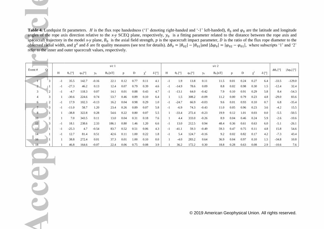
© 2019 American Geophysical Union. All rights reserved.
Table 4. Lundquist fit parameters. 𝐻 is the flux rope handedness (‘1’ denoting right-handed and ‘-1’ left-handed), 𝜃0 and 𝜑0 are the latitude and longitude
angles of the rope axis direction relative to the x-y SCEQ plane, respectively, 𝑦0 is a fitting parameter related to the distance between the rope axis and
spacecraft trajectory in the model x-y plane, 𝐵0 is the axial field strength, 𝑝 is the spacecraft impact parameter, 𝐷 is the ratio of the flux rope diameter to the
observed radial width, and χ2 and 𝛿 are fit quality measures (see text for details). ∆𝜃0 = |𝜃02| − |𝜃01|and |∆𝜑0| = |𝜑02 − 𝜑01|, where subscripts ‘1’ and ‘2’
refer to the inner and outer spacecraft values, respectively.
Event # Q
s/c 1 s/c 2
Δθ0 [°] |Δφ0| [°] H θ0 [°] φ0 [°] y0 B0 [nT] p D χ2 δ [°] H θ0 [°] φ0 [°] y0 B0 [nT] p D χ2 δ [°]
1 3 -1 35.5 142.7 -0.16 22.1 0.12 0.77 0.11 4.1 -1 1.9 13.8 0.11 11.5 0.01 0.24 0.27 6.4 -33.5 -129.0
2 1 -1 -27.3 46.2 0.13 12.4 0.07 0.79 0.39 4.6 -1 -14.9 78.6 0.09 8.8 0.02 0.98 0.30 1.5 -12.4 32.4
3 2 -1 -4.7 118.3 0.07 14.1 0.01 0.88 0.43 4.7 -1 -13.1 64.0 -0.42 7.9 0.10 0.91 0.29 5.8 8.4 -54.3
4 3 1 -30.6 224.6 0.74 53.7 0.46 0.89 0.10 6.4 1 1.5 308.2 -0.09 11.2 0.00 0.79 0.23 4.8 -29.0 83.6
6 2 -1 17.9 102.3 -0.13 16.2 0.04 0.98 0.29 1.0 -1 -24.7 66.9 -0.03 9.6 0.01 0.93 0.10 0.7 6.8 -35.4
7 3 -1 -11.0 58.7 1.20 23.4 0.26 0.89 0.07 5.8 -1 -6.9 74.3 -0.43 11.0 0.05 0.96 0.23 3.6 -4.2 15.5
8 1 1 -38.8 322.8 0.28 54.6 0.22 0.80 0.07 5.5 1 -33.4 272.4 -0.23 19.9 0.12 1.01 0.03 0.0 -5.5 -50.5
10 2 1 7.0 343.5 0.11 13.0 0.04 0.31 0.18 7.6 1 4.4 333.0 -0.26 8.9 0.04 0.46 0.24 5.9 -2.6 -10.6
12 3 -1 18.1 238.6 2.33 186.1 0.80 1.46 1.20 6.6 -1 13.0 212.5 0.94 48.4 0.36 0.61 0.63 6.0 -5.1 -26.1
13 1 -1 -25.3 4.7 -0.54 83.7 0.52 0.51 0.06 4.3 -1 -41.1 59.3 -0.49 59.3 0.47 0.75 0.11 4.8 15.8 54.6
14 1 -1 12.7 81.4 0.51 42.6 0.11 1.00 0.22 1.8 -1 5.4 124.7 -0.16 9.2 0.02 0.82 0.17 4.2 -7.3 43.4
16 1 1 38.8 272.4 0.01 37.3 0.01 1.00 0.10 0.0 1 -4.0 283.2 0.64 36.9 0.04 0.97 0.10 1.5 -34.8 10.8
18 1 1 46.8 164.6 -0.07 22.4 0.06 0.75 0.08 3.9 1 36.2 172.2 0.30 18.8 0.28 0.63 0.08 2.9 -10.6 7.6

© 2019 American Geophysical Union. All rights reserved.
Figure 1. Quality 1 ICME observations. B-field data in SCEQ coordinates at the inner spacecraft are
shown in the upper panel for each event subplot, and at the outer spacecraft in the panel below.
Where the outer spacecraft was Wind, STEREO-A or STEREO-B, the solar wind proton speed is also
displayed. Flux rope boundaries are indicated with vertical dotted lines. For ease of comparison, the
y-axis scaling for the B-field data and the x-axis timespan is the same at both spacecraft for each
event.

© 2019 American Geophysical Union. All rights reserved.
Figure 2. Quality 2 ICME observations. (Same format as Figure 1.)

© 2019 American Geophysical Union. All rights reserved.
Figure 3. Quality 3 ICME observations. (Same format as Figure 1.)

© 2019 American Geophysical Union. All rights reserved.
Figure 4. Mappings of the Quality 1 ICME profiles, in which the flux rope intervals at the inner
spacecraft have been mapped to the heliocentric distances of the outer spacecraft. Pale-colored lines
show the mapped profiles overlaying the rope intervals at the outer spacecraft, shown by the dark-
colored lines. Flux rope boundaries are indicated with vertical dotted lines.

© 2019 American Geophysical Union. All rights reserved.
Figure 5. Mappings of the Quality 2 ICME profiles. (Same format as Figure 4.)

© 2019 American Geophysical Union. All rights reserved.
Figure 6. Mappings of the Quality 3 ICME profiles. (Same format as Figure 4.)

© 2019 American Geophysical Union. All rights reserved.
Figure 7. Plots of characteristic speeds at 1 AU (x axes) versus the corresponding mean speeds (y
axes) during transit between the spacecraft. The panels show (a) the rope leading edge speeds, (b) the
center-of-mass speeds, (c) the trailing edge speeds, and (d) the expansion speeds. Dotted lines are
𝑥 = 𝑦 lines. Data-point color indicates whether the mean speeds are greater or less than the
preceding solar wind speed at 1 AU in panels (a) and (b), and greater or less than the trailing solar
wind speed at 1 AU in panel (c).
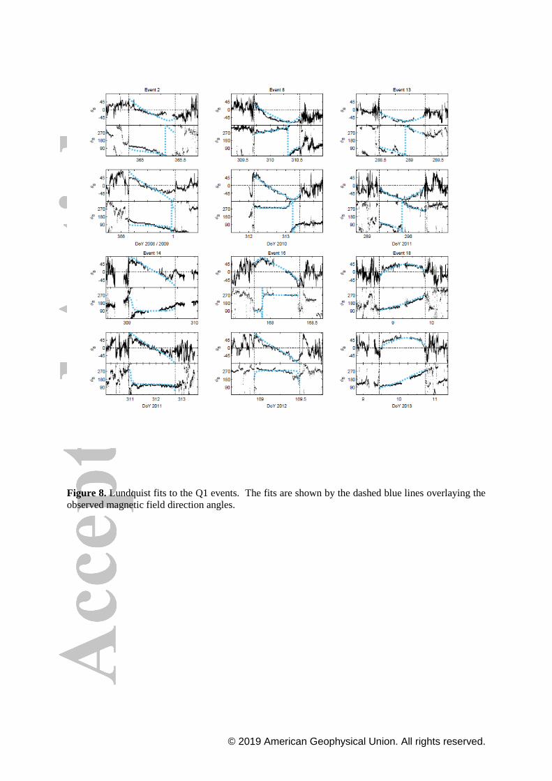
© 2019 American Geophysical Union. All rights reserved.
Figure 8. Lundquist fits to the Q1 events. The fits are shown by the dashed blue lines overlaying the
observed magnetic field direction angles.

© 2019 American Geophysical Union. All rights reserved.
Figure 9. Lundquist fit parameters versus heliocentric distance, 𝑟. The panels show (a) axis direction
latitude, (b) axis longitude direction, (c) spacecraft impact parameter, and (d) magnetic field strength
at the rope axis. Each rope is fitted independently at two radially separated locations; the dashed lines
connect the fit-value pairs for each event. In panel (a), data points for events where the rope axis
inclination relative to the solar equatorial plane (𝜃 = 0°) was lower (higher) at the outer spacecraft
compared to the inner spacecraft are colored black (red). In panel (c), data points for events where the
impact parameter was lower (higher) at the outer spacecraft are colored black (red).

© 2019 American Geophysical Union. All rights reserved.
Figure 10. Rotated mappings for Events 2 and 4, in which the mapped flux rope profiles have been
transformed such that the axis directions of the mapped flux ropes are the same as those of the ropes
observed at the outer spacecraft. Gray boxes overlaying the 𝑥-component profile for Event 2 and the
𝑦-component profile for Event 16 highlight examples of similar mesoscale features. (Same format as
Figure 4.)


![Catalog Icme Ecab[1]](https://img.pdfslide.us/doc/110x75/544c3a1caf7959a4438b59fd/catalog-icme-ecab1.jpg)