Self-exciting point processes with spatial covariates: mod

Self-exciting point processes with spatial covariates: mod-eling the dynamics of crime

Alex Reinhart and Joel GreenhouseCarnegie Mellon University, Pittsburgh, PA

E-mail: [email protected][Received August 11, 2017. Revised January 24, 2018. Final revision February 14, 2018]

Summary. Crime has both varying patterns in space, related to features of the environment,economy, and policing, and patterns in time arising from criminal behavior, such as retaliation.Serious crimes may also be presaged by minor crimes of disorder. We demonstrate that thesespatial and temporal patterns are generally confounded, requiring analyses to take both intoaccount, and propose a spatio-temporal self-exciting point process model that incorporatesspatial features, near-repeat and retaliation effects, and triggering. We develop inferencemethods and diagnostic tools, such as residual maps, for this model, and through extensivesimulation and crime data obtained from Pittsburgh, Pennsylvania, demonstrate its propertiesand usefulness.

Keywords: self-exciting point processes; predictive policing; residual maps

1. Introduction

As police departments have moved to centralized computer databases of crime reports, models topredict the risk of future crime across space and time have become widely used. Police departmentshave used predictive methods to target interventions aimed at reducing property crime (Hunt et al.,2014; Mohler et al., 2015) and violent crime (Ratcliffe et al., 2011; Taylor et al., 2011), andto analyze hotspots of robbery (Van Patten et al., 2009) and shootings (Kennedy et al., 2010),among many other applications. Predictive policing methods are now widely deployed, with lawenforcement agencies routinely making operational decisions based on them (Perry et al., 2013),and meta-analyses have shown that these policing programs can result in statistically significantcrime decreases (Braga et al., 2014).

Predictive models of crime come in several forms. The most common are tools to identify“hotspots,” small regions with elevated crime rates, using methods like kernel density estimation orhierarchical clustering on the locations of individual crimes (Levine, 2015). These tools produce

This is the peer reviewed version of the following article: A. Reinhart and J. B. Greenhouse, “Self-excitingpoint processes with spatial covariates: modelling the dynamics of crime,” Journal of the Royal StatisticalSociety: Series C (Applied Statistics), vol. 67, pp. 1305–1329, Nov 2018, which has been published in finalform at https://doi.org/10.1111/rssc.12277. This article may be used for non-commercialpurposes in accordance with Wiley Terms and Conditions for Use of Self-Archived Versions.

arX

iv:1

708.

0357

9v2

[st

at.A

P] 7

Apr

201

9

https://doi.org/10.1111/rssc.12277

2 A. Reinhart and J. Greenhouse

static hotspot maps that can be used to direct police patrols. A substantial research literaturedemonstrates that crime is highly clustered, justifying hotspot methods that identify clusters forintervention (Braga et al., 2014; Andresen et al., 2017), though these methods typically do notmodel changes in hotspots over time, even though research suggests that some hotspots emerge anddisappear over weeks or months (Gorr and Lee, 2015).

Other analysis focuses on “near-repeats”: a locally elevated risk of crime immediately after alocation experiences a crime, with the risk decaying back to the baseline level over a period ofweeks or months. Near-repeats are often analyzed using methods borrowed from epidemiologythat assess space-time clustering, such as Knox tests (Ratcliffe and Rengert, 2008; Haberman andRatcliffe, 2012), though these methods are not very fine-grained, giving only a sense of the distanceand time over which near-repeat effects are statistically significant but not the form of their decayor uncertainty in their effect. Nonetheless, near-repeat behavior has been observed for burglaries,possibly because burglars return to areas with which they are familiar (Townsley et al., 2003;Bernasco et al., 2015), and also with other types of crime, perhaps connected to gang activities andretaliation attacks (Youstin et al., 2011).

A range of regression-based analyses are also used to predict crime risks. One approach uses theincidence of “leading indicator” offenses as covariates to predict more serious crimes at later times,and taking leading indicators into account can improve predictions of crime (Cohen et al., 2007;Gorr, 2009). Leading indicators include various minor crimes, such as criminal mischief or liquorlaw violations, and police agencies can target intervention if they know which leading indicatorspredict which types of crime. On a larger scale, the “broken windows” theory states that low-leveloffenses, if not adequately controlled, lead to more serious crimes as social control disintegrates(Kelling and Wilson, 1982). Research on the broken windows hypothesis has had mixed results,suggesting the need for further tests of its predictive power (Harcourt and Ludwig, 2006; Cerdáet al., 2009).

Finally, regression is also used to assess local risk factors for crime. Risk Terrain Modeling(Kennedy et al., 2010, 2016) divides the city into a grid, regressing the number of crimes recordedin each grid cell against the presence of selected risk factors, such as gang territories, bars, high-riskhousing complexes, recent parolees, and so on. The regression output gives police a quantitativeassessment of the “risk terrain”, and enables directed interventions targeted at specific risk factors,which can more efficiently use police resources to reduce crime. The identification of risk factors isalso important for developing criminological theory to understand the nature and causes of crime(Brantingham and Brantingham, 1981).

Together, these lines of research show the range of statistical methods used to answer importantpolicing policy questions using historical crime data. In this paper, we introduce a single self-exciting point process model of crime that unifies features of all of these methods, accountingfor near-repeats, leading indicators, and spatial risk factors in a single model, and producingdynamic hotspot maps that account for change over time. We develop a range of diagnostic andsimulation tools for this model. Furthermore, we demonstrate a serious flaw in previous statisticalmethods: if leading indicators, near-repeats, and spatial features are not modeled jointly, theireffects are generically confounded. This confounding may have affected previously publishedresults. Additional simulations illustrate confounding issues that remain when some covariates areunmeasured or unknown, making it inherently difficult to interpret any spatio-temporal model.

Self-exciting point processes with spatial covariates: modeling the dynamics of crime 3

The point process model of crime proposed here extends a model introduced by Mohler et al.(2011) and refined by Mohler (2014). This model accounts for changing hotspots and near-repeatsby assuming that every crime induces a locally higher risk of crime that decays exponentially intime; hotspots, where many crimes occur in a short period of time, decay away unless sustainedcriminal activity keeps the crime intensity high. In addition, the model includes a fixed backgroundto account for chronic hotspots, and allows leading indicator crimes to contribute to the crimeintensity, with weights varying by crime type and fit by maximum likelihood. Mohler et al. (2015)demonstrated that a simplified version of this model, used to assign daily patrol priorities for a largeurban police department, can beat predictions by experienced crime analysts, leading to a roughly7.4% reduction in targeted crimes.

We extend the model proposed by Mohler (2014) to incorporate spatial features, enabling testsof criminological theory; by introducing parameter inference tools, allowing quantification of near-repeats and tests of leading indicator parameters; and with residual analysis methods, providingfine-grained analysis of model fit. The utility of the model is then demonstrated on a large dataset ofcrime from Pittsburgh, Pennsylvania. We begin by considering the confounding factors that make afull spatio-temporal model necessary.

2. Heterogeneity and state dependence

The risk of crime varies in space and time both because of spatial heterogeneity—local risk factorsfor crime, differing socioeconomic status, zoning, property development, policing patterns, localbusinesses, and so on—and through dependence on recent state, such as recent crimes that maytrigger retaliation or signal the presence of a repeat offender. In the criminological literature, theseeffects have often been studied separately, but this is problematic. A long line of research suggeststhat, in general, the effects of heterogeneity and state dependence are difficult to distinguish inobservational data and can be confounded (Heckman, 1991). We investigate this possibility in thissection, demonstrating the need for crime models that control for both effects.

Spatial heterogeneity is usually studied with tools like Risk Terrain Modeling (Kennedy et al.,2010, 2016), discussed above. At the same time, a separate line of research has focused onnear-repeat and flare-up effects, which cause short, local bursts of crime activity, with high risksstimulated by recent criminal activity. Some crimes may occur not because of features of the localenvironment but in response to recent crimes in the same area. As Johnson (2008) pointed out,however, these two effects may be confounded. If a particular neighborhood is “flagged”—thatis, has a risk factor that makes it more attractive to criminals—it will experience a higher rate ofcrime, and after any particular crime, the local risk of a repeat offense will appear to be higher thanin other parts of the city without the risk factor. But this is because of the local risk factor, notbecause the occurrence of one crime “boosted” the risk temporarily. Boosting and flagging are twosubstantively different causal theories of crime, and suggest different policies and interventions toaddress their causes, but may be difficult to distinguish from recorded crime data alone.

To distinguish between these causes, Johnson (2008) proposed a simulation approach. A virtualset of households was created, each with a baseline risk of burglary that depended on separate riskfactors, and in each interval of time, burglaries were simulated based on the risk factors. Separatesimulations were run with and without a boosting effect. Repeated across many simulations, this


Crime in i at tCrime in i at t−1

Covariate 1

Covariate 2

Fig. 1. A simplified causal diagram of crime observed in a grid cell i at two times, t and t−1, whenthere are two covariates that may affect the rate of crime.

produced patterns of near-repeats that could be compared against observed crime data, and it wasfound that the simulations containing the boost effect matched the observed data much better thanthose without. Short et al. (2009), in a similar approach, specified several different stochastic modelsof crime, and found that a model incorporating near-repeat behavior fit the observed distribution ofburglaries in Los Angeles much better than one without.

However, the ability to distinguish specific models or simulations does not imply that the twoeffects are not confounded in general. Fig. 1 gives a simplified causal diagram (Pearl, 2009) ofnear-repeat behavior in one particular grid cell i. The past occurrence of crime at time t−1 mayinfluence the rate of crime at t (the boost effect), shown by an arrow between the two, as maytwo separate risk factors, which affect the occurrence of crime at both time points (the flaggingeffect). Crucially, if the boost effect is ignored, the flagging effect of the covariates at time t isconfounded, and vice versa. It may be possible in specific simulations or in specific stochasticmodels to distinguish situations with boosting from those without, but in general, estimates of thesize of each effect will be confounded; to understand spatial risk factors we must account for theboosting, and to understand boosting we must account for the spatial risk factors.

A simple simulation can demonstrate this effect. Using the model to be introduced in Section 3.1,we simulate crimes occurring on a grid with two spatially-varying risk factors for crime, alongwith a near-repeat effect. This effect is controlled by a parameter θ, which specifies the averagenumber of crimes triggered by each occurring crime. We then perform a spatial Poisson regression,counting the simulated crimes that occurred in each grid cell and regressing against the simulatedrisk factors. The coefficients β for the intercept and risk factors are shown in Fig. 2, for simulationsranging from no near-repeat behavior (θ = 0) to a great deal of near-repeats (θ≈ 1). As near-repeatsincrease, regression coefficients gradually get more biased. The intercept, β0, increases to accountfor the additional crimes; the covariate coefficient β1 decreases from its true value of 4.8, and β2increases from its true value of −2.3. Notably, both covariate coefficients shrink towards zero in thepresence of near repeats, and the magnitude of this effect is large compared to their absolute size.

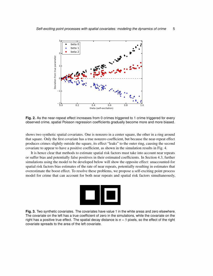
In certain circumstances, using spatial risk factors with particular patterns, near-repeats cancause false positives: risk factors that appear related to crime rates but are not. For example, Fig. 3


0.0 0.2 0.4 0.6 0.8 1.0theta (self-excitation)

2

1

0

1

2

3

Devia

tion f

rom

tru

e p

ara

mete

r

beta 0beta 1beta 2

Fig. 2. As the near-repeat effect increases from 0 crimes triggered to 1 crime triggered for everyobserved crime, spatial Poisson regression coefficients gradually become more and more biased.

shows two synthetic spatial covariates. One is nonzero in a center square, the other in a ring aroundthat square. Only the first covariate has a true nonzero coefficient, but because the near-repeat effectproduces crimes slightly outside the square, its effect “leaks” to the outer ring, causing the secondcovariate to appear to have a positive coefficient, as shown in the simulation results in Fig. 4.

It is hence clear that methods to estimate spatial risk factors must take into account near repeatsor suffer bias and potentially false positives in their estimated coefficients. In Section 4.3, furthersimulations using the model to be developed below will show the opposite effect: unaccounted-forspatial risk factors bias estimates of the rate of near repeats, potentially resulting in estimates thatoverestimate the boost effect. To resolve these problems, we propose a self-exciting point processmodel for crime that can account for both near repeats and spatial risk factors simultaneously,

Fig. 3. Two synthetic covariates. The covariates have value 1 in the white areas and zero elsewhere.The covariate on the left has a true coefficient of zero in the simulations, while the covariate on theright has a positive true effect. The spatial decay distance is σ = 5 pixels, so the effect of the rightcovariate spreads to the area of the left covariate.


0.0 0.2 0.4 0.6 0.8 1.0theta (self-excitation)

4

3

2

1

0

1

2

3

4

5

Devia

tion f

rom

tru

e p

ara

mete

r

beta 0beta 1beta 2

Fig. 4. As the amount of self-excitation increases, the coefficient β1 (the left covariate in Fig. 3)increases from zero, despite its true value being zero. β2 shrinks toward zero for the same reasonas in Fig. 2.


eliminating the confounding.

3. Methods

3.1. Self-exciting point process modelSelf-exciting point process models are a class of models for spatio-temporal point process data thatincorporate “self-excitation”: each event may excite further events, by locally increasing the eventrate for some period of time. This corresponds to the near repeat phenomenon we need to accountfor. Self-exciting point processes are a development of Hawkes processes (Hawkes, 1971), whichare purely temporal processes. The theory and applications of self-exciting spatio-temporal pointprocesses were reviewed by Reinhart (2018); we give only a brief summary here.

A spatio-temporal point process is characterized by its conditional intensity function, definedfor locations s ∈ X ⊆ Rd and times t ∈ [0,T ) as

λ(s, t |Ht) = lim∆s,∆t↓0

E[N(B(s,∆s)× [t, t +∆t)

)|Ht

]|B(s,∆s)|∆t

, (1)

where |B(s,∆s)| is the Lebesgue measure of the ball B(s,∆s) with radius ∆s, N(A) is the countingmeasure of events over the set A⊆ X× [0,T ), and Ht is the history of events in the process up totime t. In the limit, the conditional intensity can be interpreted as the instantaneous rate of eventsper unit time and area, and hence the expected number of events in time interval [t1, t2) and regionB is

E[N(B× [t1, t2))] =∫ t2

t1

∫B

λ(s, t)dsdt.

Self-exciting point processes have conditional intensities of the form

λ(s, t |Ht) = µ(s)+ ∑i:ti<t

g(s− si, t− ti)

= µ(s)+∫ t

0

∫X

g(s−u, t− r)dN(u× r),

where g is a triggering function that determines the form of the self-excitation. In the remainder ofthis paper, we will refer to λ(s, t) without the explicit Ht to simplify notation, but λ(s, t) should stillbe understood to depend on the past history of the process.

Models of this form have been widely used in a variety of processes exhibiting clustering, suchas earthquake epicenters (Ogata, 1999) and the occurrence of infectious diseases (Meyer et al.,2012; Meyer and Held, 2014). Mohler et al. (2011) developed such a model for the occurrence ofviolent crime by building on the models used in earthquake forecasting, known in the seismologyliterature as epidemic-type aftershock sequence models (Ogata, 1999). This model allows hotspotestimates to change over time by separating crime into chronic hotspots, which remain fixed intime, and temporary hotspots, which are caused by increases or changes in crime. (In seismologicalmodels, earthquakes are similarly divided into main shocks and aftershocks triggered by those mainshocks.) Hotspot intensities are modeled with a modification of kernel density smoothing, where


past crimes contribute to the intensity with effects that decay away in time, and the bandwidthparameters are estimated to best fit the data instead of being chosen by the operator.

Mohler (2014) further adapted the model to include leading indicator crimes, producing a modelthat predicts the conditional intensity λ(s, t) of crime at each location s and time t as the sum of abackground rate and a sum of functions of prior crimes:

λ(s, t) = µ(s)+ ∑all events i

before time t

g(s− si, t− ti,Mi), (2)

where µ(s) is a background crime rate that does not vary in time, and si and ti are locations andtimes of other crimes used as leading indicators. Mi represents the type of each leading indicatorcrime, as different indicators are allowed to have different predictive effects in this model.

The triggering function g is defined to be

g(s, t,M) =θMω

2πσ2 exp(−ωt)exp

(−‖s‖

2

2σ2

),

where σ2 is the bandwidth, θM determines how much each type of leading indicator contributes tothe intensity, and the effect decays exponentially in time with a rate controlled by ω. Because gis chosen to integrate to θM, it has a natural interpretation: the expected number of target crimesinduced by a single leading indicator crime of type M.

Mohler (2014) chose the background crime rate µ(s) to be a sum of weighted Gaussian kernelscentered at prior crimes:

µ(s) = ∑i

αMi

2πη2Texp

(−‖s‖

2

2η2

). (3)

Here αMi determines the contribution of each leading indicator type to the background rate, η2 isthe bandwidth, and T is the total length of time over which the crime data falls.

This model has several limitations. The background component (3) does not explicitly accountfor varying spatial features or give estimates of their effects, and the use of weighted Gaussiankernels for both g(s, t,M) and µ(s) makes the model parameters difficult to identify; to preventmultiple modes in the log-likelihood, Mohler (2014) had to set σ = η.

We have extended this model to replace the nonparametric µ(s) with one that directly incorporatesspatial covariate information, allowing estimates of the effects of each covariate and avoidingidentifiability issues. We assume that the observation domain X is divided into cells c of arbitraryshape, inside of which a covariate vector Xc (including an intercept term) is known, resulting in themodel

λ(s, t) = exp(

βXC(s)

)+ ∑

i:ti<tg(s− si, t− ti,Mi), (4)

where C(s) is the index of the covariate cell containing s and the triggering function g is unchanged.We let g(s, t,M) = 0 for s < δ, for an arbitrary short distance δ, to prevent crimes that occur atexactly the same location from enticing the model to converge to σ = 0.

In principle, this model could be built with covariates that vary continuously in space, definedby a function X(s). This would increase the generality of the model. However, in practice, this


generality is not necessary: most socioeconomic, demographic, or land use variables are observedonly in cells such as city blocks, census blocks, or neighborhoods. Piecewise constant covariatesalso make estimation and simulation more computationally tractable, and so the small loss ingenerality is worth the substantial gain in practicality.

We may also reasonably ask about the form of the triggering function g, which specifies anexponential decay in time and a Gaussian kernel in space. Meyer and Held (2014), for example,analyzing the spread of infectious disease, proposed a power law kernel to account for long-rangeflows of people. Unfortunately, most alternate spatial kernels make the expectation maximizationstrategy described below more difficult, by making analytical maximization on each iterationimpossible. These kernels could still be used, but with the additional computational cost ofnumerical maximization.

3.2. Simulation algorithmSimulations from self-exciting point process models have proved useful both for examining infer-ence and for the simulation studies discussed in Sections 2 and 4. Various simulation algorithms forself-exciting point processes were discussed by Reinhart (2018, Section 3.3). We chose to use analgorithm introduced by Zhuang et al. (2004) for earthquake aftershock sequence models, which isfast and efficient for our model structure. This algorithm draws on a key property of self-excitingpoint processes shown by Hawkes and Oakes (1974): a self-exciting process can be represented asa cluster process. Cluster centers come from an inhomogeneous Poisson process with rate µ(s), andeach cluster center produces a cluster of offspring events with locations and times determined bythe triggering function g(s, t,M). Each of these offspring events may trigger further offspring of itsown, and so on.

This leads to a natural simulation procedure that first draws from the inhomogeneous Poissoncluster center process, then draws a generation of offspring based on those cluster centers, andrepeats until there are no more offspring. Full details are given by Zhuang et al. (2004). Drawsfrom the cluster center process are made easier by our assumption that the observation domainis divided into cells c, inside each of which is a constant covariate vector Xc; we can hence drawcluster centers from homogeneous Poisson processes inside each cell.

Our simulation system can simulate from the model specified by eq. (4), but can also simulatevarious violations of assumptions: the spatial distribution of offspring can be Gaussian, t witharbitrary degrees of freedom, Cauchy, or various other shapes, and their temporal distribution canbe drawn from an exponential distribution or a Gamma distribution with arbitrary parameters. Theframework is flexible and allows additional distributions to be chosen easily; this feature will beused in Section 4.2 to test model performance under various types of misspecification.

3.3. Parameter inferenceMohler (2014) fit the self-exciting model by maximum likelihood, using the log-likelihood functionfor spatio-temporal point processes:

`(Θ) = ∑i

logλ(si, ti)−∫ T

0

∫X

λ(s, t)dsdt, (5)


where X is the spatial domain of the observations and Θ a complete vector of parameters. Thelog-likelihood is optimized via expectation maximization, using the approximation that X = R2 tosimplify calculation of the triple integral, which is valid when most crime triggered by the observedcrimes occurs within the study area (Schoenberg, 2013). Note that, as the model predicts the targetcrime and not the leading indicators, only the target crimes are included in the sum in Eq. (5). Weadapted the expectation maximization procedure to fit our extended model.

The expectation maximization procedure for self-exciting processes was first described by Veenand Schoenberg (2008), and follows the general procedure described by Reinhart (2018, Section3.1). A latent variable ui is introduced for each event i, indicating whether the event came fromthe background process (ui = 0) or was triggered by a previous event j (ui = j). Augmented withthis variable, the log-likelihood simplifies from the form in (5), since the intensity λ(si, ti) no longerinvolves a sum over the background µ(s) and all previous events but only the term indicated by ui.We can then take the expectation and maximize. In our model, maximization proceeds in closedform for most parameters, apart from β, which must be separately numerically maximized on eachiteration.

Mohler (2014) did not provide inference for the self-exciting point process model parameters,though they may be of interest: the self-excitation parameters σ2, ω, and θ may be used to testhypotheses about the concentration of crime and the nature of leading indicators. Mohler’s non-parametric background (3) also does not incorporate spatial covariates, though β in our backgroundindicates the association between spatial covariates and crime. There are several potential routes toderiving asymptotic confidence intervals for these parameters, which we consider in turn.

First, Rathbun (1996) demonstrated the asymptotic normality and consistency of the maximumlikelihood estimator for spatiotemporal point processes:

√T (Θ−Θ) u N(0,Σ) as T → ∞, where

u represents uniform convergence in distribution and Θ is the complete vector of parameters.The result holds under certain regularity conditions on the conditional intensity. Rathbun (1996)suggested an estimator for the covariance matrix Σ of the parameter estimate Θ,

V (Θ) =

(Nc

∑i=1

∆(si, ti)λ(si, ti)

)−1

,

where ∆(s, t) is a matrix-valued function with elements

∆i j(s, t) =

∂

∂Θiλ(s, t) ∂

∂Θ jλ(s, t)

λ(s, t). (6)

With the full estimated covariance matrix, we calculated standard errors for each estimator, andproduced confidence intervals from these.

An alternate approach, following again from the asymptotic normality result, is to use theobserved information matrix at the maximum likelihood estimate, based on the Hessian of thelog-likelihood:

Σ =−H(Θ)−1,

where H(Θ) is the matrix of second partial derivatives of `(Θ) evaluated at Θ. This approach wassuggested by Ogata (1978) in the context of an asymptotic normality result for temporal point


Table 1. Coverage of nominal 95% CIs

Variable Hessian (%) Rathbun (%)

σ2 86 88ω 87 91θ 82 63β0 77 83β1 89 92β2 86 89

Average 85 88

processes, and has been frequently used for spatio-temporal models in seismology; however, Wanget al. (2010), comparing its estimated standard errors with those found by repeated simulation,found that it can be heavily biased for smaller samples.

Nonetheless, we implemented the estimator using Theano (Bergstra et al., 2010), a Pythonpackage for describing computations that automatically generates fast C code and automaticallycomputes all necessary derivatives. We then performed a series of 350 simulations to compare thefinite-sample performance of both estimators with our model, using randomly chosen parametervalues, obtaining the results shown in Table 1. Coverage is worst for the self-excitation parametersσ2, ω, and θ, which are affected by any remaining boundary effect (see Section 4.1) not compensatedfor by the buffer region; Rathbun’s covariance estimator achieves nearly nominal coverage for β,which is less affected. Overall, Rathbun’s estimator achieves 88% coverage and is closest to itsnominal 95% coverage. We will use this estimator in our analysis in Section 5.

3.4. Residual analysisOnce a model is fit, it is useful to be able to determine where the model fits: what types of systematicdeviations are present, where covariates may be lacking, what types of crimes are over- or under-predicted, and so on. Eq. (1) suggests we can produce these detailed analyses: because the pointprocess model predicts a conditional intensity at each location, we can calculate the expectednumber of crimes within each region in a certain period of time, and compare this against the trueoccurrences over the same time, producing a residual map. These residuals are defined to be (Daleyand Vere-Jones, 2008, chapter 15)

R(h) =∫R×R2

h(s, t)[N(ds×dt)−λ(s, t)dt ds

],

where N(·) is the counting measure of events in the given region, and h(s, t) is a bounded windowfunction. Typically, h(s, t) is taken to be an indicator function for a chosen spatio-temporal region.

To calculate R(h), a typical approach is to choose a time window [t1, t2)—say, a particularweek or month—and integrate the conditional intensity over this window, producing an integratedintensity function

λ(s) =∫ t2

t1λ(s, t)dt.


Then the spatial region X is divided appropriately and the intensity is integrated over each subdivi-sion, then compared against the number of events in that subdivision during that time window.

Choosing spatial subdivisions for residuals requires care. The obvious choice is a discrete grid,but the right size is elusive: small grid cells produce skewed residuals with high variance (as mostcells have no crimes), and positive and negative residual values can cancel each other out in largecells. Bray et al. (2014) instead suggest instead using the Voronoi tessellation of the plane, whichproduces a set of convex polygons, known as Voronoi cells, each of which contains exactly onecrime and all locations that are closer to that crime than to any other.

Given this tessellation, the raw Voronoi residuals ri for each cell Ci are

ri = 1−∫

Ci

λ(s)ds.

The choice of Voronoi cells ensures that cell sizes adapt to the distribution of the data, and Brayet al. (2014) cite extensive simulations by Tanemura (2003) indicating that the Voronoi residuals ofa homogeneous Poisson process have an approximate distribution given by

ri ∼ 1−X , where X ∼ Gamma(3.569,3.569),

so that E[ri] = 0. (Here the gamma distribution is parametrized by its shape and rate.) But becausethe conditional intensity function (4) is not homogeneous, we performed similar simulations forrandom parameter values, fitting to 1,332,546 simulated residuals by maximum likelihood theapproximate distribution X ∼ Gamma(3.389,3.400).

After each ri is found, using Monte Carlo integration over Ci, the Voronoi cells can be mappedwith colors corresponding to their residual values. To ease interpretation, colors are determined by−Φ−1(F(1− ri)) where F is the cumulative distribution function of the approximate distribution ofX and Φ−1 the inverse normal cdf. Positive residuals hence indicate more observed crime than waspredicted, and negative residuals less.

These residual maps provide much more detailed information than previous global measures ofhotspot fit, and can indicate areas with unusual patterns of criminal activity. For example, considera model that predicts homicides using leading indicators such as assault and robbery; this modelmay perform well in an area that experiences gang-related violence, but would systematicallyover-predict homicides in a commercial area full of bars and nightclubs, where most assaults aredrunken arguments rather than signs of gang conflict. An example residual map is given in Fig. 12(Section 5.2) for Pittsburgh burglary data, illustrating the use of this method.

The example map does illustrate one weakness of Voronoi residual maps. We would expectareas with large positive residuals (red, in the map) to have a higher crime density than areas withlarge negative residuals (blue), since positive residuals indicate more crimes occurred than wereexpected. Hence areas with positive residuals tend to have smaller Voronoi cells than areas withnegative residuals, and the map is visually dominated by large cells with negative residuals. Closerinspection reveals clusters of very small cells containing large positive residuals; these are thelocations of new crime hotspots. Users should be aware of this problem when interpreting residualmaps.

We have also introduced animated residual videos. Instead of a single time window [t1, t2),we produce a succession of windows {[t1 +(i− 1)δt , t1 + iδt) : i = 1,2,3 . . .}. For each window,


we calculate the Voronoi tessellation of crimes occurring in that window and the correspondingresiduals r j. These residuals, and the times of the events defining each cell, are used to build asmoothed residual field similar to that suggested by Baddeley et al. (2005). The residual valueat each animation frame and each point in space is determined by a kernel smoother, using anexponential kernel in time and a Gaussian kernel in space, with the same structure as the triggeringfunction g(s, t). An animated version of Fig. 12 is provided in the Supplemental Materials as anexample.

A purely temporal residual analysis can be useful to illustrate the calibration of the model overtime. Consider plotting the index i of each event versus the quantity

τi =∫ ti

0

∫X

λ(s, t)dsdt,

the expected number of events in the interval [0, ti). This is an extension of the standard transfor-mation property of point processes: if the model is correct, the resulting process {τi} will be astationary Poisson process with intensity 1 (Papangelou, 1972). Hence the plotted points will fallon the diagonal, and by plotting the deviation from the diagonal, poor calibration becomes obvious.Similar diagnostics have previously been used for seismological models (e.g. Ogata, 1988). Anexample of this diagnostic will be shown in Section 4.3, demonstrating its use in detecting someforms of model misspecification.

3.5. Prediction evaluationTo compare different methods for locating crime hotspots, fairly simple metrics have been typicallyused, such as the hit rate: the percentage of crimes during the test period that occur inside theselected hotspots. A modified version is the Prediction Accuracy Index (PAI), which dividesthe hit rate by the total fraction of the map that is selected as hotspots, to penalize methods thatachieve their accuracy by simply selecting a larger total land area (Chainey et al., 2008). However,this still requires selecting a single set of hotspots, and in some simulations, we found the PAIwas maximized by shrinking the denominator, selecting a single 100 meter grid cell containingseveral crimes as the only hotspot. This is hardly practical, and says little about the comparativeperformance of models. The conditional intensity function λ(s, t) provides much richer information:the estimated rate of crime at every location at all times. We would like a metric that is maximizedwhen λ(s, t) neither underestimates nor overestimates the true crime rate.

Such a metric can be found with proper scoring rules (Gneiting and Raftery, 2007), whichhave previously been used for self-exciting point process models in seismology (Vere-Jones, 1998).Scoring rules evaluate probabilistic forecasts of events: a score S(P,x) returns the score of apredictive distribution P when outcome x occurs. A scoring rule S is proper if the expected value ofS(P,x) is maximized by P when x is drawn from P. An example of a proper score is the logarithmicscore S(P,x) = log px, where px is the forecast probability of event x under the predictive distributionP. The expected value of the logarithmic score, under a particular P, can be interpreted as thepredictability of the outcome x, and is related to the entropy of the distribution.

Harte and Vere-Jones (2005), noting this connection, proposed a method for comparing differentpredictive models. The relative entropy of a predictive distribution P compared to a baseline


distribution π isI∗ = EP log

px

πx,

where π is a simple default distribution, such as a homogeneous Poisson process model, againstwhich all models are compared. Applied to a self-exciting point process model, we may produceP by performing one-step predictions: after each event, form a predictive distribution for the nextevent. Because the predictive distribution P is conditional on the past history of the point process,I∗ is random, depending on the particular realization of the process; the average over all possiblerealizations G = E[I∗] is called the expected information gain, and numerically quantifies theintrinsic predictability of the process.

A further connection soon becomes apparent. If we perform this one-step prediction process foreach event in a point process realization, the logarithmic score for each event is the log-likelihood ofthat event, and the relative entropy I∗ is the expected log-likelihood ratio. The expected informationgain G is hence estimated by the log-likelihood ratio on an observed dataset:

G =1T

logL1/L0, (7)

where L0 is the baseline model likelihood and L1 the likelihood of the model of interest. Thelikelihood ratio between two models hence estimates the difference in score between them, in theform of the relative entropy. (The theoretical aspects here were reviewed in more depth by Daleyand Vere-Jones (2004).) This quantity an be used to compare the predictive performance of modelson test time periods.

Further, this quantity can be connected to the difference in Akaike Information Criterion (AIC)between the two models (Harte and Vere-Jones, 2005). If the baseline model has k0 parameters andthe model of interest has k1 parameters, the difference in AIC can be written as

∆AIC2T

=k1− k0

T− G,

where ∆AIC = 2(k1− k0)− 2logL1/L0. This suggests the use of ∆AIC to compare the predic-tive performance of models with varying number of parameters, which will be demonstrated inSection 5.2.

4. Simulation studies

4.1. Boundary effectsAs noted by Zhuang et al. (2004) and Reinhart (2018), boundary effects can be a problem if eventsare only observed in a subset of the space, such as if crimes are only recorded inside a specificjurisdiction. If crimes are only observed in the region X and time interval [0,T ), but also occuroutside X and at t < 0 or t ≥ T , maximum likelihood parameter estimates can be biased by boundaryeffects. Unobserved crimes just outside X or before t = 0 can produce near repeats that are observed,and observed crimes near the boundary of X can stimulate near repeats outside the boundary thatare not. This biases model fits to underestimate the rate of near repeats.


These boundary effects are distinct from boundary effects in kernel density estimation (e.g.Cowling and Hall, 1996), which bias density estimates near the boundary. Similar problems occurhere, with λ(s, t) biased near the boundary of X , but additional biases on parameter estimates occur.The nature of these boundary effects can be seen clearly from the parameter updates in the M stepof the EM algorithm. For example, the update step for θL is

θL =∑responses i ∑t j<ti P(ui = j)I(M j = L)

KL−∑crimes i I(Mi = L)e−(T−ti)/ω,

which can be interpreted as a weighted average: for all crimes of type L, sum up their contributionsto response crimes (measured by P(ui = j)), and take the average. An average of 0.5, for example,says a crime of type L can be expected to contribute to about 0.5 future response crimes. Thedenominator also contains a temporal boundary correction term that is negligible when T is verylarge.

Suppose, however, that many crimes of type L occur near the boundary of the observation regionX , and trigger response crimes that occur outside of X . These response crimes will not be includedin the sum in the numerator, and hence θL will be biased downward. Updates for σ2 and ω can alsobe interpreted as weighted averages, and are subject to similar biases.

Harte (2012) explored the effects of these biases on the seismological models. One commonworkaround to reduce the bias is to introduce a region X0 ⊂ X , chosen so that events inside X0 havetriggered offspring that mostly occur within X . All events in X contribute to the intensity λ(s, t),but the weighted averages in the M step only average over events inside X0: that is, to update θL, weaverage over events of type L within X0, counting their contributions to any response crimes withinX . Since most of their offspring will be within X by construction, the average will not leave muchout.

The same subsetting is also done in time, so only events in the interval [0,T0) are considered,where T0 < T . This eliminates bias caused by events at t close to T triggering offspring that occurafter T and are hence not observed.

Of course, averaging over events only in a subset of space and time reduces the effective samplesize of the fit, introducing additional variance to parameter estimates. It does, however, dramaticallyreduce bias. To demonstrate this, Table 2 shows parameter values obtained from 50 simulationsfrom a model with known parameter values, with two covariates. The true parameters are θ = 0.5,ω = 7 days, and σ = 4 feet; the covariate coefficients are β1 = 1.2 and β2 = −1.5. The grid is66×60 feet and no boundary correction was applied, resulting in the biases shown. Note that θ isbiased too low, since events triggered outside the grid were not observed, and both ω and σ are alsotoo small. The covariate coefficients are both biased towards zero because the intercept increased toaccount for the events no longer accounted for by θ.

The third column of Table 2 shows the average fit obtained when an 8-foot boundary wasestablished around the images, so X0 was the inner 50×44 box; the simulated events occurred overthe course of two years, of which the last thirty days were also left out. These fits suffer from muchless bias.


Table 2. Average parameter values withand without boundary correction

Parameter Uncorrected Corrected

θ 0.3367 0.4706ω 6.104 days 6.638 daysσ2 3.173 feet 3.913 feetβ0 (intercept) -19.65 -19.78β1 1.135 1.176β2 -1.348 -1.498

Long tails Reference0.5

1.0

1.5

2.0

2.5

3.0 1e 5 Information gain

Fig. 5. Boxplot of information gains (eq. (7)) obtained from fits to simulated data with Cauchy-distributed offspring (left) or Gaussian offspring (right). The poor fit from model misspecification isnoticeable.

4.2. Model misspecificationIn this section we explore the results of model misspecification on the fit, to determine whenmisspecification may be detected and corrected. As an example, consider two simulations: onein which event offspring are drawn from the Gaussian g used in fitting our model, and one inwhich event offspring are drawn from a Cauchy distribution, giving them a heavy tail that is notaccounted for by our model. Running 100 simulations under each condition and calculating the log-likelihoods of fits to each, we obtained the information gains G shown in Fig. 5, which demonstratethe deterioration in model fit when misspecified. In this situation, the disturbance in model fit islimited to the self-excitation parameters θ and ω (σ2 is not meaningful to compare here), alongwith the intercept β0; the estimates of β for the simulated covariates are unaffected, suggesting thatmisspecification of the triggering function need not harm inference about the spatial covariates.

We performed several other simulations of different forms of misspecification, using boxcarand double exponential spatial distributions and also a Gamma distribution for offspring times.With spatial misspecification, the covariate coefficients were still unbiased on average, with slightbiases in θ depending on the type of misspecification, and larger biases in ω (towards longer decaytimes). Misspecification of the offspring timing did not bias θ, β, or ω, but did cause systematic


Crime in i at tCrime in i at t−1

Covariate 1 Covariate 2

Fig. 6. A simplified causal diagram depicting potential confounding: covariate 1 has a causalrelationship with both covariate 2 and crime rates, and so if it is unobserved, estimates of covariate2’s effect will be confounded.

understimation of σ2. These results suggest that the covariate coefficient estimates of the model arerobust to misspecification of the self-excitation component, though the self-excitation parameterscan be sensitive to misspecification, giving misleading estimates of cluster size and duration.

4.3. Unobserved covariates and confoundingSection 2 discussed the inherent confounding that can occur when estimating the effect of spatialcovariates on crime without accounting for self-excitation. Fig. 1 demonstrated that this confoundingis generic, occurring whenever there are covariates that affect crime over time. By building a self-exciting point process model that accounts for self-excitation and covariates, we can account forboth and avoid the confounding.

We must, however, be aware of other types of confounding that can creep in. The most commonis an unobserved covariate: there are many spatial factors that can influence crime rates, and it isunlikely we can directly measure all of them. Fig. 6 demonstrates the danger. A covariate may becausally related to another covariate as well as to crime rates, and if it is not observed and accountedfor, the other covariate’s estimated effect will be confounded. This is directly analogous to thesituation in ordinary regression, when unobserved predictors may confound regression coefficientestimates.

On the other hand, if the two covariates are not correlated in any way, omitting one does notbias estimates of the other’s effect; in traditional regression its mean effect is simply added tothe intercept and the individual effects simply add to the error variance. However, in the morecomplicated self-exciting point process model, omitted covariates may have other detrimental effects.Though Schoenberg (2016) suggests that parameter estimates remain asymptotically consistentwhen covariates are omitted, provided the effects of those covariates are sufficiently small, a seriesof simulations demonstrate the bias that appears in finite samples.

We generated covariates on a grid, drawing the covariate values from a Gaussian process withsquared exponential covariance function to ensure there was some spatial structure. We first ran100 simulations (each with new Gaussian process draws) of independent covariates, fitting a modelwith both covariates included and one with the second covariate omitted, each using the expectationmaximization procedure described in Section 3.3. Simulations were performed with random trueparameter values, and these values were recorded, along with the fits. It is apparent from the resultsthat estimates of θ are affected by the missing covariate: Fig. 7 shows the fits, as a function of the


6 4 2 0 2 4 6true beta2

1.0

0.5

0.0

0.5

true t

heta

0 -

est

imate

d t

heta

0

Both covariates included

6 4 2 0 2 4 6true beta2

true t

heta

0 -

est

imate

d t

heta

0

Covariate 2 omitted

Fig. 7. The difference between the true value of θ and the estimated value, as a function of thecoefficient β2, when the two covariates are independent. On the left, fits made when β2 is accountedfor; on the right, when it is not. Notice the odd behavior around β2 = 0: when the omitted covariatedoes not matter, θ is estimated to be close to its true value, but when it has a larger effect, θ hasmuch higher variance.

true value of β2 used in the simulation, and a distinct pattern can be seen when the second covariateis omitted from the fit, with θ having larger variance for larger values of |β2|. On average, theestimated θ with a missing covariate is larger than the true θ by 0.18.

Overestimation of θ has other consequences. For example, Fig. 8 shows a temporal residual plot(see Section 3.4) for a fit to a simulated dataset with an omitted covariate. An obvious calibrationproblem is present: by the time the 500th event occurred, the conditional intensity function predicted150 fewer events than occurred. Near t = 0, λ(s, t) cannot predict the observed events because thereis little past history of events; near t = T , a long past history and overestimated θ causes λ(s, t) tooverestimate the intensity and “catch up” in the cumulative predicted number of events.

Additionally, the time decay parameter ω is also overestimated by 70% on average. Together,these biases suggest that the clustering induced by the unobserved covariate is being accountedfor by increasing self-excitation and by allowing the effects of self-excitation to last longer in themodel.

Next, we simulated causally confounded covariates, following the causal model in Fig. 6.Covariate 1 was drawn from a Gaussian process, as before, and Covariate 2 was defined to bethe average of Covariate 1 and a separate independent Gaussian process. This gave an averagecorrelation of r = 0.66 between the covariates. Sample correlated covariates are shown in Fig. 9.Data was simulated from these covariates (with random coefficients) and then models fit with andwithout Covariate 2 included. Fig. 10 demonstrates the bias in estimates of β1 that ensues when theeffect of β2 is not accounted for, similar to the biases that can occur in ordinary linear regressionwhen covariates are confounded. The confounding also affects θ and ω in a similar way as in the


0 1000 2000 3000Incident index

150

125

100

75

50

25

0Di

ffere

nce

from

inte

grat

ed in

tens

ityTemporal residuals

Fig. 8. Temporal residual plot for a simulated fit with a missing covariate, demonstrating the effectof the overestimated θ.

previous simulation, with bias as |β2| increases.Together, these simulations demonstrate two important caveats of self-exciting point process

models:

(a) Omitted spatial covariates, whether or not they are confounded with observed covariates, canbias estimates of the self-excitation parameter θ, making it seem as though events are morelikely to trigger offspring events.

(b) Omitted spatial covariates can also bias estimates of the temporal decay parameter ω, makingit seem as though self-excitation or near-repeat effects occur over a longer timescale than theyreally do.

(c) If there is a confounding relationship between covariates, such as that shown in Fig. 6,unobserved covariates can bias estimates of observed covariate effects (β) as well as ofself-excitation.

The first two points are particularly concerning, since in practical applications it is unlikely thatall covariates could ever be accounted for—there will always be unmeasured spatial differencesin base rates, or imperfectly measured covariates. This suggests that previous applications of self-exciting point process models may have overestimated the amount and time scale of self-excitationin the process, unless their background estimator was able to capture all spatial variation in baserates.


0 5 10 15 200

5

10

15

20Covariate 1

20

40

60

80

100

120

140

Rate

per

tim

e p

er

gri

d c

ell

0 5 10 15 200

5

10

15

20Covariate 2

3

6

9

12

15

18

21

24

27

Rate

per

tim

e p

er

gri

d c

ell

Fig. 9. The rate induced (that is, exp(βX), where β = 1 for simplicity and X is the covariate) by twoGaussian process covariates on a 20×20 grid. The second covariate is dependent upon the first.Notice the spatial structure of the Gaussian process.

6 4 2 0 2 4 6true beta2

10

5

0

5

10

true b

eta

1 -

est

imate

d b

eta

1

Both covariates included

6 4 2 0 2 4 6true beta2

true b

eta

1 -

est

imate

d b

eta

1

Covariate 2 omitted

Fig. 10. Bias observed in estimated values of β1 when β2 is also estimated (left) or is omitted fromthe fit (right).


In some cases, the residual analyses introduced in Section 3.4 may make it possible to detectwhen there is an important unobserved spatial covariate. Temporal residual plots like Fig. 8 cansuggest the presence of unobserved covariates (or other misspecification), while residual maps canmake systematic deviations from the predicted event rate visible, and careful examination of themaps may suggest variables that need to be included. Section 5 gives examples of this in Pittsburghcrime data.

General approaches to account for unobserved covariates are more difficult. One strategy,sometimes used in spatial regressions, is to include a spatial random effect term intended to accountfor the unobserved covariates. However, at least in spatial regression, this method does not achieveits goal: a spatial random effect can bias coefficients of the observed covariates in arbitrary ways,particularly if the unobserved covariate is spatially correlated with any of the observed covariates(Hodges and Reich, 2010). Given the causal diagram in Fig. 1, it does not seem possible for any oneadjustment to account for an unobserved covariate and give unbiased estimates of the effects of theother covariates. Users of spatial regression and the self-exciting point process model introducedhere need to be aware of their limitations in the presence of unobserved confounders, and interpretresults carefully.

5. Application

5.1. Pittsburgh incident dataTo demonstrate the spatio-temporal model of crime proposed here, we will analyze a database of205,485 police incident records filed by the Pittsburgh Bureau of Police (PBP) between June 1,2011, and June 1, 2016, specifying the time and type of each incident and the city block on which itoccurred. (Privacy regulations prevent PBP from releasing the exact addresses or coordinates ofcrimes, so PBP provides only the coordinates of the block containing the address.) The recordsinclude crimes from very minor incidents (such as 38 violations of Pittsburgh’s ordinance againstspitting) to violent crimes, such as homicides and assaults. Only crimes reported to PBP areincluded, so the dataset does not include records from the police departments of Pittsburgh’s severalmajor universities, including the University of Pittsburgh, Carnegie Mellon University, ChathamUniversity, or Carlow University.

Because the database contains only incident reports, offense types are preliminary. Chargeslisted in the reports may be downgraded or dropped, suspects acquitted, or new charges filed. Thereports represent only the charges reported by the initial investigating officers, so they may notcorrespond with final FBI Uniform Crime Report data or other sources. While this limits theaccuracy of our data, it is also the only practical approach—final charges may not be known formonths, so predictions based on them would be hopelessly out of date.

Rather than dealing with the numerous sections and subsections of the Pennsylvania CriminalCode represented in the incident data, we used the FBI Uniform Crime Report hierarchy, whichsplits incident types into a common hierarchy comparable across states and jurisdictions. Amongso-called “part I” crimes, homicide, assault, and rape are at the top of the hierarchy, followed byother crimes like theft, burglary, and so on. If an incident involves two distinct types of crime (e.g.a burglary involving an assault on a homeowner), we use the type higher in the hierarchy, followingthe FBI’s “Hierarchy Rule” (FBI, 2004). The hierarchy of offenses is shown in Table 3. In our


Table 3. The part I crime hierarchy

Hierarchy Crime Count

1 Homicide 3002 Forcible rape 8933 Robbery 58844 Aggravated assault 59005 Burglary 119436 Larceny/theft 374877 Motor vehicle theft 38928 Arson 0

analysis we focused on crimes in these categories, though other “part II” crimes, such as simpleassault and vandalism, are also available in the dataset, along with every other offense type recordedby the Pittsburgh Bureau of Police. Note that arson, typically hierarchy level 8, was miscoded inthe data available to us, though arson was not used in any of our analyses.

We also collected, from city and Census Bureau data, various spatial covariates for each Censusblock, including

• The fraction of residents who are male from age 18–24

• The fraction of residents who are black

• The fraction of homes that are occupied by their owners, rather than rented

• The total population

• Population density (per square meter)

• The fraction of residents who are black or Hispanic.

Some city blocks have no population (e.g. in commercial areas with no residents), so anadditional dummy variable was used to record whether each block had a population. In all modelsthat follow, population-based covariates only enter the models when the block has a nonzeropopulation.

These covariates will be used to demonstrate the model’s ability to account for spatial factorsthat attract crime. They are not intended to be a comprehensive list of all possible risk factors, andundoubtedly there are other relevant covariates; systematic identification and evaluation of relevantspatial features is out of the scope of this work.

5.2. Burglary analysisSelecting only the first year of burglary data, containing 2892 burglaries, we fit two models, oneusing only population density as a covariate and the other using additional covariates. The burglariesare mapped in Fig. 11, showing spatial structure in the locations of burglary hotspots across thecity. The model fits are shown in Table 4 and Table 5. Asymptotically normal 95% confidence


1

mi

Burglaries, 2011-06-01 to 2012-06-01

Fig. 11. Locations of 2892 burglaries recorded in Pittsburgh between June 1, 2011 and June 1,2012

intervals based on Rathbun’s covariance estimator are also shown for each parameter. The additionalcovariates improve the model AIC from 179750 to 179319, an improvement of about 431 units.Notice the relative consistency of the self-excitation parameters ω and σ2 between fits, and that, asexpected from the discussion in Section 4.3, θ decreases when additional covariates are added.

Interpretation of the model with all covariates (Table 5) is straightforward. Each burglarystimulates or predicts, on average, θ = 0.59 further burglaries, distributed with a spatial bandwidthof σ≈ 468 feet at a rate exponentially decaying in time with parameter ω≈ 47 days. High populationdensities predict higher risks of burglary, as there are more residences to burgle; similarly, blockswith populations greater than zero (a proxy for residential vs. commercial blocks) have a higherburglary rate. The remaining covariates enter the model when blocks have a population greater thanzero. Higher proportions of young men indicate a lower burglary risk, though the confidence intervalfor this effect overlaps zero. Home ownership, rather than renting, has a negative effect, while ahigher fraction of black residents is correlated with higher burglary rates; these last two factors arelikely confounded with poverty and socioeconomic status, which have strong relationships withcrime but are not included in this model.

For a larger view of Pittsburgh, Fig. 12 shows an overall residual map of Pittsburgh overtwo months. Several trends appear, suggesting inadequacies in the available covariates and the


Table 4. Predicting burglary using population density

Parameter Value CI

θ 0.764 [0.717, 0.811]ω 4.511×106 (52.21 days) [47.04, 57.39]σ2 2.664×105 (516.1 feet) [487.2, 543.5]β0 (intercept) -31.63 [-31.50, -31.76]β1 (pop / m2) 31.66 [8.91, 54.4]

AIC 179750

Table 5. Predicting burglary using additional covariates

Parameter Value CI

θ 0.589 [0.544, 0.635]ω 4.061×106 (47.00 days) [41.97, 52.04]σ2 2.194×105 (468.4 feet) [439.0, 496.1]β0 (intercept) -33.15 [-33.53, -32.78]β1 (pop / m2) 25.50 [6.13, 44.86]β2 (block populated?) 2.49 [2.05, 2.92]β3 (frac. male 18–24) -0.69 [-1.74, 0.36]β4 (frac. black) 0.75 [0.55, 0.95]β5 (frac. homes owned) -1.14 [-1.40, -0.88]

AIC 179319


Fig. 12. Residual map from the fit shown in Table 4, over two months of burglaries. A: downtown, B:University of Pittsburgh, C: Carnegie Mellon University.

presence of boundary effects: commercial areas such as downtown (at the confluence of the tworivers) have fewer burglaries than predicted, and the presence of the University of Pittsburgh andCarnegie Mellon University also results in negative residuals, as each has its own police departmentwhose records are not included in our dataset. Note that, as discussed in Section 3.4, negative(blue) residuals visually dominate, because areas with lower-than-expected crime hence have largerVoronoi cells; also note the presence of several clusters of small cells with large positive residuals,at the locations of temporary burglary hotspots.

To demonstrate leading indicators, we fit an additional model containing the same set ofcovariates but also two leading indicators, larceny/theft and motor vehicle theft (hierarchy levels 6and 7). The fit is shown in Table 6, and shows that motor vehicle theft in particular seems predictiveof burglary, with a coefficient of θ2 = 0.1167. The AIC of this model further improved to 179201,by 118 units.

Temporal calibration plots for these models show patterns similar to Fig. 8, suggesting, asdiscussed in Section 4.3, that there is additional spatial heterogeneity in crime rates which isnot accounted for by the available covariates in these models, and hence that the self-excitation


Table 6. Predicting burglary with leading indicators

Parameter Value CI

θ0 (self-excitation) 0.4480 [0.404, 0.492]θ1 (larceny/theft) 0.0632 [0.049, 0.078]θ2 (motor vehicle theft) 0.1167 [0.037, 0.197]ω 3.551×106 (41.10 days) [36.5, 45.8] daysσ2 1.619×105 (402.3 feet) [376, 427] feetβ0 (intercept) -33.90 [-34.47, -33.33]β1 (pop / m2) 25.19 [2.48, 47.9]β2 (block populated?) 3.00 [2.37, 3.63]β3 (frac. male 18–24) -0.85 [-2.14, 0.43]β4 (frac. black) 0.94 [0.72, 1.15]β5 (frac. homes owned) -1.00 [-1.30, -0.71]

AIC 179201

parameters may be overestimates. Further research is necessary to identify relevant covariates andprepare higher-resolution covariate datasets to adequately model crime.

6. Conclusions

Self-exciting point processes have been used for a wide range of applications, from epidemiologyto seismology, and we have built on this work to introduce an improved model for crime, extendingprevious crime models by incorporating spatial covariate information and providing parameterinference tools to aid understanding of the patterns of crime. Though self-exciting point processmodels are more complex than ordinary spatial regression, making analysis more difficult forusers used to the wealth of tools available for regression, we have helped bridge this gap throughinterpretable residual diagnostic tools (adapted from related models) and through scoring methodsfor comparing the predictive performance of models, neither of which has previously been usedwith any crime hotspot analysis tool.

A contribution of our work is a demonstration, both theoretically and through simulations, thatmethods that focus purely on the spatial or temporal aspects of crime are generally confounded andcan produce misleading results, requiring a method that accounts for both aspects simultaneously.This calls into doubt previous results on the connection of spatial features to crime, and the problemgeneralizes to self-exciting processes outside of crime, such as models of infectious disease andearthquakes. Extensive simulations characterize our model’s reaction to misspecification andomitted covariates, both likely problems to experience in real-world data.

Together, the tools and simulations presented in this paper provide a single comprehensivepackage of modeling, diagnostic, and inference tools for self-exciting point processes, which havenot previously been assembled in one place. The model and tools will enable new criminologicalresearch, revealing patterns of crime, allowing tests of theories about the origin and dynamics ofcrime, and contributing to improved policing strategies. Additional research will more extensivelyexplore the Pittsburgh crime dataset, along with other cities, and additional covariates and types


of crime. Further, the tools and results described here apply beyond the analysis of crime, to anyspatio-temporal process with self-excitation.

Acknowledgments

Thanks to Daniel S. Nagin for criminological advice, and to Evan Liebowitz for compiling the Pitts-burgh spatial covariate data. We thank the anonymous referees for suggestions which substantiallyimproved the manuscript.

This work was supported by Award No. 2016-R2-CX-0021, awarded by the National Instituteof Justice, Office of Justice Programs, U.S. Department of Justice. The opinions, findings, andconclusions or recommendations expressed in this publication are those of the authors and do notnecessarily reflect those of the Department of Justice.

References

Andresen, M. A., Linning, S. J. and Malleson, N. (2017) Crime at Places and Spatial Concentrations:Exploring the Spatial Stability of Property Crime in Vancouver BC, 2003–2013. Journal of QuantitativeCriminology, 33, 255–275.

Baddeley, A., Turner, R., Møller, J. and Hazelton, M. (2005) Residual analysis for spatial point processes(with discussion). Journal of the Royal Statistical Society: Series B (Statistical Methodology), 67, 617–666.

Bergstra, J., Breuleux, O., Bastien, F., Lamblin, P., Pascanu, R., Desjardins, G., Turian, J., Warde-Farley, D.and Bengio, Y. (2010) Theano: a CPU and GPU math expression compiler. In Proceedings of the Pythonfor Scientific Computing Conference (SciPy).

Bernasco, W., Johnson, S. D. and Ruiter, S. (2015) Learning where to offend: Effects of past on futureburglary locations. Applied Geography, 60, 120–129.

Braga, A. A., Papachristos, A. V. and Hureau, D. M. (2014) The Effects of Hot Spots Policing on Crime: AnUpdated Systematic Review and Meta-Analysis. Justice Quarterly, 31, 633–663.

Brantingham, P. J. and Brantingham, P. L. (1981) Environmental Criminology. SAGE Publications.Bray, A., Wong, K., Barr, C. D. and Schoenberg, F. P. (2014) Voronoi residual analysis of spatial point process

models with applications to California earthquake forecasts. Annals of Applied Statistics, 8, 2247–2267.Cerdá, M., Tracy, M., Messner, S. F., Vlahov, D., Tardiff, K. and Galea, S. (2009) Misdemeanor policing, phys-

ical disorder, and gun-related homicide: a spatial analytic test of "broken-windows" theory. Epidemiology,20, 533–541.

Chainey, S., Tompson, L. and Uhlig, S. (2008) The Utility of Hotspot Mapping for Predicting Spatial Patternsof Crime. Security Journal, 21, 4–28.

Cohen, J., Gorr, W. L. and Olligschlaeger, A. M. (2007) Leading Indicators and Spatial Interactions: ACrime-Forecasting Model for Proactive Police Deployment. Geographical Analysis, 39, 105–127.

Cowling, A. and Hall, P. (1996) On pseudodata methods for removing boundary effects in kernel densityestimation. Journal of the Royal Statistical Society Series B, 58, 551–563.

Daley, D. J. and Vere-Jones, D. (2008) An Introduction to the Theory of Point Processes, Volume II: GeneralTheory and Structure, vol. 2. Springer, 2 edn.

Daley, D. T. and Vere-Jones, D. (2004) Scoring Probability Forecasts for Point Processes: The Entropy Scoreand Information Gain. Journal of Applied Probability, 41, 297–312.

FBI (2004) Uniform Crime Reporting Handbook. Department of Justice. URL: https://ucr.fbi.gov/additional-ucr-publications/ucr_handbook.pdf.

https://ucr.fbi.gov/additional-ucr-publications/ucr_handbook.pdf

https://ucr.fbi.gov/additional-ucr-publications/ucr_handbook.pdf


Gneiting, T. and Raftery, A. E. (2007) Strictly Proper Scoring Rules, Prediction, and Estimation. Journal ofthe American Statistical Association, 102, 359–378.

Gorr, W. L. (2009) Forecast accuracy measures for exception reporting using receiver operating characteristiccurves. International Journal of Forecasting, 25, 48–61.

Gorr, W. L. and Lee, Y. (2015) Early Warning System for Temporary Crime Hot Spots. Journal of QuantitativeCriminology, 31, 25–47.

Haberman, C. P. and Ratcliffe, J. H. (2012) The Predictive Policing Challenges of Near Repeat Armed StreetRobberies. Policing, 6, 151–166.

Harcourt, B. E. and Ludwig, J. (2006) Broken Windows: New Evidence from New York City and a Five-CitySocial Experiment. The University of Chicago Law Review, 73, 271–320.

Harte, D. and Vere-Jones, D. (2005) The Entropy Score and its Uses in Earthquake Forecasting. Pure andApplied Geophysics, 162, 1229–1253.

Harte, D. S. (2012) Bias in fitting the ETAS model: a case study based on New Zealand seismicity. Geophysi-cal Journal International, 192, 390–412.

Hawkes, A. G. (1971) Spectra of some self-exciting and mutually exciting point processes. Biometrika, 51,83–90.

Hawkes, A. G. and Oakes, D. (1974) A Cluster Process Representation of a Self-Exciting Process. Journal ofApplied Probability, 11, 493–503.

Heckman, J. J. (1991) Identifying the hand of past: Distinguishing state dependence from heterogeneity.American Economic Review, 81, 75–79.

Hodges, J. S. and Reich, B. J. (2010) Adding Spatially-Correlated Errors Can Mess Up the Fixed Effect YouLove. The American Statistician, 64, 325–334.

Hunt, P., Saunders, J. and Hollywood, J. S. (2014) Evaluation of the Shreveport Predictive Policing Experiment.RAND.

Johnson, S. D. (2008) Repeat burglary victimisation: a tale of two theories. Journal of ExperimentalCriminology, 4, 215–240.

Kelling, G. L. and Wilson, J. Q. (1982) Broken windows: The police and neighborhood safety. AtlanticMonthly, 127, 29–38.

Kennedy, L. W., Caplan, J. M. and Piza, E. L. (2010) Risk Clusters, Hotspots, and Spatial Intelligence: RiskTerrain Modeling as an Algorithm for Police Resource Allocation Strategies. Journal of QuantitativeCriminology, 27, 339–362.

Kennedy, L. W., Caplan, J. M., Piza, E. L. and Buccine-Schraeder, H. (2016) Vulnerability and Exposure toCrime: Applying Risk Terrain Modeling to the Study of Assault in Chicago. Applied Spatial Analysis andPolicy, 9, 529–548.

Levine, N. (2015) CrimeStat: A Spatial Statistics Program for the Analysis of Crime Incident Locations (v4.02). Ned Levine & Associates and the National Institute of Justice.

Meyer, S., Elias, J. and Höhle, M. (2012) A Space-Time Conditional Intensity Model for Invasive Meningo-coccal Disease Occurrence. Biometrics, 68, 607–616.

Meyer, S. and Held, L. (2014) Power-law models for infectious disease spread. Annals of Applied Statistics,8, 1612–1639.

Mohler, G. O. (2014) Marked point process hotspot maps for homicide and gun crime prediction in Chicago.International Journal of Forecasting, 30, 491–497.

Mohler, G. O., Short, M. B., Brantingham, P. J., Schoenberg, F. P. and Tita, G. E. (2011) Self-Exciting PointProcess Modeling of Crime. Journal of the American Statistical Association, 106, 100–108.


Mohler, G. O., Short, M. B., Malinowski, S., Johnson, M., Tita, G. E., Bertozzi, A. L. and Brantingham,P. J. (2015) Randomized controlled field trials of predictive policing. Journal of the American StatisticalAssociation, 110, 1399–1411.

Ogata, Y. (1978) The asymptotic behaviour of maximum likelihood estimators for stationary point processes.Annals of the Institute of Statistical Mathematics, 30, 243–261.

— (1988) Statistical models for earthquake occurrences and residual analysis for point processes. Journal ofthe American Statistical Association, 83, 9–27.

— (1999) Seismicity Analysis through Point-process Modeling: A Review. Pure and Applied Geophysics,155, 471–507.

Papangelou, F. (1972) Integrability of expected increments of point processes and a related random change ofscale. Transactions of the American Mathematical Society, 165, 483–483.

Pearl, J. (2009) Causal inference in statistics: An overview. Statistics Surveys, 3, 96–146.Perry, W. L., McInnis, B., Price, C. C., Smith, S. C. and Hollywood, J. S. (2013) Predictive Policing: The

Role of Crime Forecasting in Law Enforcement Operations. RAND Corporation.Ratcliffe, J. H. and Rengert, G. F. (2008) Near-Repeat Patterns in Philadelphia Shootings. Security Journal,

21, 58–76.Ratcliffe, J. H., Taniguchi, T., Groff, E. R. and Wood, J. D. (2011) The Philadelphia foot patrol experiment:

A randomized controlled trial of police patrol effectiveness in violent crime hotspots. Criminology, 49,795–831.

Rathbun, S. L. (1996) Asymptotic properties of the maximum likelihood estimator for spatio-temporal pointprocesses. Journal of Statistical Planning and Inference, 51, 55–74.

Reinhart, A. (2018) A review of self-exciting spatio-temporal point processes and their applications. StatisticalScience.

Schoenberg, F. P. (2013) Facilitated estimation of ETAS. Bulletin of the Seismological Society of America,103, 601–605.

— (2016) A note on the consistent estimation of spatial-temporal point process parameters. Statistica Sinica,26, 861–879.

Short, M. B., D’Orsogna, M. R., Brantingham, P. J. and Tita, G. E. (2009) Measuring and Modeling Repeatand Near-Repeat Burglary Effects. Journal of Quantitative Criminology, 25, 325–339.

Tanemura, M. (2003) Statistical distributions of Poisson Voronoi cells in two and three dimensions. Forma,18, 221–247.

Taylor, B., Koper, C. S. and Woods, D. J. (2011) A randomized controlled trial of different policing strategiesat hot spots of violent crime. Journal of Experimental Criminology, 7, 149–181.

Townsley, M., Homel, R. and Chaseling, J. (2003) Infectious burglaries: A test of the near repeat hypothesis.British Journal of Criminology, 43, 615–633.

Van Patten, I. T., McKeldin-Coner, J. and Cox, D. (2009) A Microspatial Analysis of Robbery: ProspectiveHot Spotting in a Small City. Crime Mapping, 1, 7–32.

Veen, A. and Schoenberg, F. P. (2008) Estimation of space–time branching process models in seismologyusing an em–type algorithm. Journal of the American Statistical Association, 103, 614–624.

Vere-Jones, D. (1998) Probabilities and Information Gain for Earthquake Forecasting. ComputationalSeismology, 30, 248–263.

Wang, Q., Schoenberg, F. P. and Jackson, D. D. (2010) Standard Errors of Parameter Estimates in the ETASModel. Bulletin of the Seismological Society of America, 100, 1989–2001.

Youstin, T. J., Nobles, M. R., Ward, J. T. and Cook, C. L. (2011) Assessing the Generalizability of the NearRepeat Phenomenon. Criminal Justice and Behavior, 38, 1042–1063.


Zhuang, J., Ogata, Y. and Vere-Jones, D. (2004) Analyzing earthquake clustering features by using stochasticreconstruction. Journal of Geophysical Research, 109, B05301.

Documents

Self-exciting point processes with spatial covariates: mod