Embed Size (px)
Citation preview
Otto-von-Guericke-Universitat Magdeburg
Faculty of Computer Science
DS EB
Databases
SoftwareEngineering
and
Master’s Thesis
Self-Driving Vertical Partitioningwith Deep Reinforcement Learning
Author:
Rufat Piriyev
February, 8th, 2019
Advisors:
M.Sc. Gabriel Campero Durand
Data and Knowledge Engineering Group
Prof. Dr. rer. nat. habil. Gunter Saake
Data and Knowledge Engineering Group

Piriyev, Rufat:Self-Driving Vertical Partitioning with Deep Reinforcement LearningMaster’s Thesis, Otto-von-Guericke-Universitat Magdeburg, 2019.
Abstract
Selecting the right vertical partitioning scheme is one of the core database optimizationproblems. It is especially significant because when the workload matches the partitioning,the processing is able to skip unnecessary data, and hence it can be faster [Bel09]. Duringthe last four decades numerous different algorithms have been proposed to reach efficientlythe optimal vertical partitioning. Mainly these algorithms rely on two aspects. Onone side, cost models, which approximate how well a workload might be supportedwith a given configuration. On the other side, they rely on pruning heuristics thatare able to narrow down the combinatorial search space, trading optimality for lesserruntime complexity [GCNG16]. Nowadays modified and improved variations of thesemethods can be expected to be included in commercial DBMSs [ANY04b, JQRD11](although precise information on the solutions used by commercial systems are keptconfidential [BAA12a]). Nonetheless, though these methods are efficient, they do notemploy any machine learning technique, and thus are unable to improve their performancebased on previous executions, nor are they able to be learn from cost-model errors.
Deep reinforcement learning (DRL) methods could address these limitations, whilestill providing an optimal and timely solution. In our research we aim to evaluate thefeasibility of using DRL methods for self-driving vertical partitioning. To this end wepropose a novel design that maps the process from the current domain to the domainof DRL. Furthermore, we validate our design experimentally by studying the trainingand the inference process for a given TPC-H data and workload, on a prototype weimplement using Open AI Gym, and the Google Dopamine framework for DRL.
We train 3 different DQN agents for bottom-up partitioning with 3 selected cases: afixed workload and table, a set of fixed workload and tables, and finally a fixed tablewith a random workload. We find that convergence is easily achievable for the first twoscenarios, but that generalizing to random workloads requires further work. In addition,we report the impact of hyperparameters in the convergence.
Regarding inference we compare the predictions of our agents with that of state-of-the-artalgorithms like HillClimb, AutoPart and O2P [JPPD], finding that our agents haveindeed learned the optima during the training carried out. We also report competitiveruntimes for our agents on both GPU and CPU inference, which are able to outperformsome state of the art algorithms, and the brute-force algorithm as the table size increases.

iv

Acknowledgements
First of all, I would like to thank my supervisor M.Sc. Gabriel Campero Durand forintroducing me to this challenging topic. Without his permanent guidance, patienceand constant encouragement this work could not have been possible.
I would like to thank Prof. Dr. rer. nat. habil. Gunter Saake for giving me theopportunity to write my Master’s thesis with the DBSE research group.
I would like to thank M.Sc. Marcus Pinnecke for assisting us in finding a computer withGPU support for our long-running experiments.
I would like to thank M.Sc. David Broneske, M.Sc. Sabine Wehnert, Mahmoud Mohsenand others for their constructive feedback which I found very useful during my work.
Special thanks to the team of SAP UCC Magdeburg and Dr. Pape Co. ConsultingGmbH for allowing me to take a break during the last phase of this thesis.
Finally, I would like to thank my family, relatives and friends for their continuoussupport during my studies.

vi

Declaration of Academic Integrity
I hereby declare that this thesis is solely my own work and I have cited all externalsources used.
Magdeburg, February 8th 2019
———————–Rufat Piriyev

Contents
List of Figures xii
1 Introduction 11.1 Motivation . . . . . . . . . . . . . . . . . . . . . . . . . . . . . . . . . . . 11.2 Our contributions . . . . . . . . . . . . . . . . . . . . . . . . . . . . . . . 51.3 Research Methodology . . . . . . . . . . . . . . . . . . . . . . . . . . . . 51.4 Thesis structure . . . . . . . . . . . . . . . . . . . . . . . . . . . . . . . . 7
2 Background 92.1 Horizontal and vertical partitioning . . . . . . . . . . . . . . . . . . . . . 92.2 Vertical partitioning algorithms . . . . . . . . . . . . . . . . . . . . . . . 11
2.2.1 Navathe . . . . . . . . . . . . . . . . . . . . . . . . . . . . . . . . 142.2.2 O2P . . . . . . . . . . . . . . . . . . . . . . . . . . . . . . . . . . 162.2.3 AutoPart . . . . . . . . . . . . . . . . . . . . . . . . . . . . . . . 182.2.4 HillClimb . . . . . . . . . . . . . . . . . . . . . . . . . . . . . . . 19
2.3 Reinforcement learning . . . . . . . . . . . . . . . . . . . . . . . . . . . . 212.3.1 RL basics . . . . . . . . . . . . . . . . . . . . . . . . . . . . . . . 21
2.3.1.1 Basic components of RL models . . . . . . . . . . . . . . 222.3.1.2 Q-learning and SARSA . . . . . . . . . . . . . . . . . . 242.3.1.3 ε-greedy and Boltzmann exploration strategies . . . . . . 24
2.3.2 Deep RL . . . . . . . . . . . . . . . . . . . . . . . . . . . . . . . . 252.3.2.1 Deep Q-Network (DQN) . . . . . . . . . . . . . . . . . . 272.3.2.2 Basic extensions to DQN . . . . . . . . . . . . . . . . . 282.3.2.3 Distributional RL . . . . . . . . . . . . . . . . . . . . . . 292.3.2.4 Rainbow . . . . . . . . . . . . . . . . . . . . . . . . . . . 30
2.4 Summary . . . . . . . . . . . . . . . . . . . . . . . . . . . . . . . . . . . 31
3 Self-driving vertical partitioning with deep reinforcement learning 333.1 Architecture of our solution . . . . . . . . . . . . . . . . . . . . . . . . . 333.2 Grid World Environment . . . . . . . . . . . . . . . . . . . . . . . . . . . 353.3 Summary . . . . . . . . . . . . . . . . . . . . . . . . . . . . . . . . . . . 39
4 Experimental setup 414.1 Research Questions . . . . . . . . . . . . . . . . . . . . . . . . . . . . . . 42
x Contents
4.2 Hyper-parameters for DQN agents . . . . . . . . . . . . . . . . . . . . . . 424.3 Unified settings for proposed algorithms . . . . . . . . . . . . . . . . . . 454.4 Measurement Process . . . . . . . . . . . . . . . . . . . . . . . . . . . . . 464.5 Experiment Environment . . . . . . . . . . . . . . . . . . . . . . . . . . . 464.6 Benchmark . . . . . . . . . . . . . . . . . . . . . . . . . . . . . . . . . . 474.7 Summary . . . . . . . . . . . . . . . . . . . . . . . . . . . . . . . . . . . 48
5 Evaluation and Results 495.1 Training of models . . . . . . . . . . . . . . . . . . . . . . . . . . . . . . 49
5.1.1 Complexity of learning instance . . . . . . . . . . . . . . . . . . . 505.1.2 Convergence in case of fixed workload and tables . . . . . . . . . 505.1.3 Convergence in case of fixed workload and table pairs . . . . . . . 535.1.4 Case of fixed table and random workload . . . . . . . . . . . . . . 59
5.2 Algorithms comparison . . . . . . . . . . . . . . . . . . . . . . . . . . . . 625.2.1 Generated partitions . . . . . . . . . . . . . . . . . . . . . . . . . 625.2.2 Inference times . . . . . . . . . . . . . . . . . . . . . . . . . . . . 65
5.3 Summary . . . . . . . . . . . . . . . . . . . . . . . . . . . . . . . . . . . 68
6 Related Work 69
7 Conclusion and Future work 757.1 Conclusion . . . . . . . . . . . . . . . . . . . . . . . . . . . . . . . . . . . 75
7.1.1 Threats to validity . . . . . . . . . . . . . . . . . . . . . . . . . . 767.2 Future work . . . . . . . . . . . . . . . . . . . . . . . . . . . . . . . . . . 77
A Structural views of using agents, derived from Tensorboard 79
B Hyper-parameters used for each agent 83B.1 DQN agent parameters . . . . . . . . . . . . . . . . . . . . . . . . . . . . 83B.2 Implicit Quantile agent parameters . . . . . . . . . . . . . . . . . . . . . 84B.3 Rainbow agent parameters . . . . . . . . . . . . . . . . . . . . . . . . . . 85
C Inference times 87
Bibliography 89
List of Figures
1.1 CRISP-DM Process Diagram . . . . . . . . . . . . . . . . . . . . . . . . 6
2.1 Example of horizontal partitioning . . . . . . . . . . . . . . . . . . . . . 10
2.2 Example of vertical partitioning . . . . . . . . . . . . . . . . . . . . . . . 11
2.3 Initial attribute affinity matrix (AA); (b) attribute affinity matrix insemiblock diagonal form; (c) non-overlapping splitting of AA into twoblocks L and U ([72]). . . . . . . . . . . . . . . . . . . . . . . . . . . . . 15
2.4 Outline of the partitioning algorithm used by AutoPart ([PA04a]). . . . 18
2.5 The AutoPart algorithm ([PA04a]). . . . . . . . . . . . . . . . . . . . . 19
2.6 The Agent-Environment interaction in MDP . . . . . . . . . . . . . . . . 21
2.7 Taxonomy of recent RL algorithms . . . . . . . . . . . . . . . . . . . . . 26
2.8 Network architectures of different Deep RL algorithms, derived from[DOSM18] . . . . . . . . . . . . . . . . . . . . . . . . . . . . . . . . . . . 30
3.1 The architecture of our proposed solution, adapted from the originalDopamine architecture . . . . . . . . . . . . . . . . . . . . . . . . . . . . 34
3.2 An example of state merging . . . . . . . . . . . . . . . . . . . . . . . . . 38
3.3 REST API response example . . . . . . . . . . . . . . . . . . . . . . . . 39
4.1 Proposed NN architecture . . . . . . . . . . . . . . . . . . . . . . . . . . 43
4.2 TPC-H database . . . . . . . . . . . . . . . . . . . . . . . . . . . . . . . 47
5.1 Single table, Blue line - DQN agent, Red line - Rainbow agent, Greenline - Implicit quantile agent . . . . . . . . . . . . . . . . . . . . . . . . 51
5.2 Single table learning . . . . . . . . . . . . . . . . . . . . . . . . . . . . . 52
5.3 Update horizon tuning . . . . . . . . . . . . . . . . . . . . . . . . . . . . 54
xii List of Figures
5.4 . . . . . . . . . . . . . . . . . . . . . . . . . . . . . . . . . . . . . . . . . 55
5.5 Hard and soft updates, UH=3, with pruning actions . . . . . . . . . . . . 57
5.6 Bolztmann and ε-greedy strategies (Soft update, UH=3, with pruningactions) . . . . . . . . . . . . . . . . . . . . . . . . . . . . . . . . . . . . 58
5.7 Average training time for agents . . . . . . . . . . . . . . . . . . . . . . . 59
5.8 Evaluation plot for random workflow case, with trendline . . . . . . . . . 60
5.9 Training plot for random workload case . . . . . . . . . . . . . . . . . . . 61
5.10 Number of episodes per iteration for random workload case . . . . . . . . 61
5.11 Customer and Lineitem tables with corresponding costs for each algorithm 62
5.12 Supplier and Region tables with corresponding costs for each algorithm . 63
5.13 Part and PartSupp tables with corresponding costs for each algorithm . . 64
5.14 Nation and Orders tables with corresponding costs for each algorithm . . 65
5.15 Inference times for LineItem and Customer tables (seconds) . . . . . . . 66
5.16 Inference times for the remaining 6 tables (seconds) . . . . . . . . . . . . 67
6.1 The ReJOIN framework [MP18] . . . . . . . . . . . . . . . . . . . . . . 72
6.2 State representation. RL schema[OBGK18] . . . . . . . . . . . . . . . . 73
A.1 DQN agent, structural view derived from Tensorboard. . . . . . . . . . . 80
A.2 Implicit quantile agent, structural view derived from Tensorboard. . . . 81
A.3 Rainbow agent, structural view derived from Tensorboard. . . . . . . . . 82
C.1 Inference times for default TPC-H table-workload pairs (seconds) . . . . 88
1. Introduction
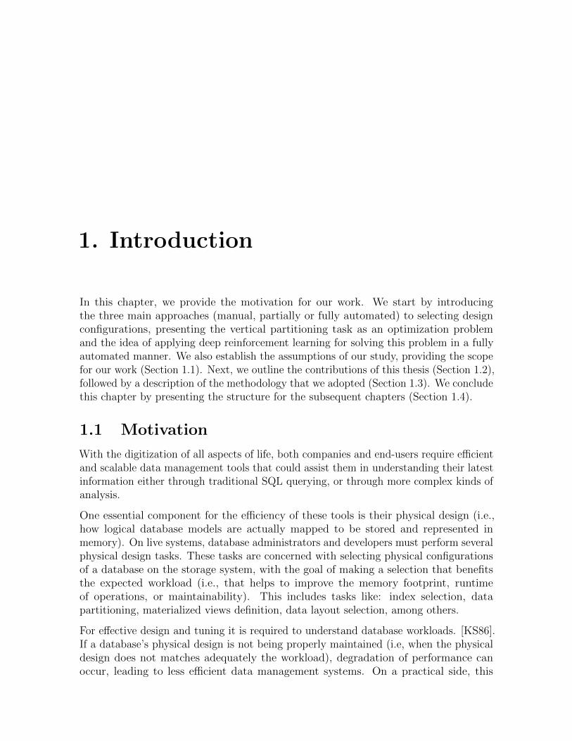
In this chapter, we provide the motivation for our work. We start by introducingthe three main approaches (manual, partially or fully automated) to selecting designconfigurations, presenting the vertical partitioning task as an optimization problemand the idea of applying deep reinforcement learning for solving this problem in a fullyautomated manner. We also establish the assumptions of our study, providing the scopefor our work (Section 1.1). Next, we outline the contributions of this thesis (Section 1.2),followed by a description of the methodology that we adopted (Section 1.3). We concludethis chapter by presenting the structure for the subsequent chapters (Section 1.4).
1.1 Motivation
With the digitization of all aspects of life, both companies and end-users require efficientand scalable data management tools that could assist them in understanding their latestinformation either through traditional SQL querying, or through more complex kinds ofanalysis.
One essential component for the efficiency of these tools is their physical design (i.e.,how logical database models are actually mapped to be stored and represented inmemory). On live systems, database administrators and developers must perform severalphysical design tasks. These tasks are concerned with selecting physical configurationsof a database on the storage system, with the goal of making a selection that benefitsthe expected workload (i.e., that helps to improve the memory footprint, runtimeof operations, or maintainability). This includes tasks like: index selection, datapartitioning, materialized views definition, data layout selection, among others.
For effective design and tuning it is required to understand database workloads. [KS86].If a database’s physical design is not being properly maintained (i.e, when the physicaldesign does not matches adequately the workload), degradation of performance canoccur, leading to less efficient data management systems. On a practical side, this
2 1. Introduction
implies that when considering rapidly changing workloads, database administrators anddevelopers face several challenges, such as: evaluating at great speed a high number ofpossible configurations to determine the best, dealing with possible correlation betweenconfigurable parameters[VAPGZ17], and finally facing to the uncertainty of predictingthe impact of configurations by using cost models and assumptions that might not fullymatch the real-world database system (i.e., as happens for other database choices, likejoin order optimization with mistaken cardinality estimates[Loh14]).
To alleviate these challenges research has proposed two approaches that extend thepurely manual configuration management (i.e., the case where database administratorsand developers are not supported for configuring the system). The first approach is theuse of partially automated tools, such as database tuning advisors, which recommenddatabase administrators certain configurations based on an expected workload[ABCN06].This is usually done in a batch-wise fashion. The second approach is the use of fullyautomated solutions. From this last group solutions can either follow a heuristic-drivenapproach, which means that they do not use machine learning models and are based ondomain-specific knowledge; or they can adopt a self-driving approach, which proposesto let the database itself deal with configuration choices automatically[PAA+17], in anonline manner, by using machine learning models and letting the optimizers learn fromtheir mistakes, without involving the database administrators.
Tools produced by the first approach have been shown to create difficulties for databaseadministrators, such as inaccurate estimates or failures in modeling update costs, creatingunpredictable results [BAA12b].
The second approach, and specifically the self-driving design, though still in activedevelopment, seems specially promising as it could speed the time-to-deployment ofconfiguration changes and, through the use of continuous learning, it could addressfailures of partially automated solutions.
In this thesis we research on the task of developing a self-driving tool to aid in a specificphysical design case which, to date, has mostly been studied following a batch-wise,either heuristic-driven or partially automated approach: vertical partitioning. This is theproblem of finding the optimal combination of column groups (i.e., vertical partitions),for an expected database workload. This choice is highly relevant, since it can achieveto optimize the amount of data that needs to be considered by a workload, helping toavoid the loading of unnecessary column groups.
Vertical partitioning is not a new optimization problem, and researchers have offeredmany different algorithms and solutions during the last forty years, like one of the firstworks by Hammer and Niamir[HN79a]. At its core, this optimization problem consistsof evaluating with a cost model the combinatorial space of possible column groupingsand determining which solution is estimated to be the best.
One of the biggest problems that algorithmic solutions face here is to find the righttrade-off between the robustness of the solution (i.e., optimality) and optimizationcomplexity[JPPD]. There are many popular non-machine learning based approaches
1.1. Motivation 3
for choosing the optimal vertical partition in a database relation, by using differentheuristics that prune the search space of possible solutions that are evaluated.
For our study, following the goal of adopting a machine learning solution to this problem,we propose to study the applicability of a reinforcement learning (RL) model for mappinga traditional vertical partitioning solution to a self-driving solution. RL is one of the threemain types of machine learning (i.e., apart from supervised and unsupervised learning),where models are trained using a system of rewards, obtained through interactions withan environment. Here RL is intended to aid in helping the model to navigate efficientlya search space, by learning the long-term value of a given action in a state; such thatafter a model is trained, online predictions can be made without exploring the completesearch space. In specific, we decompose the recommendation for a complete partitioningscheme, into the recommendation of piece-wise actions (in a discrete action space) thatwhen applied, should result in increasing improvements in the partitioning scheme and,by the end of our recommendations, in an optimal partitioning.
However, there are challenges in adopting a traditional RL solution: On one hand, thechallenge of learning over a large action-state space (as the number of columns increases),which, in the absence of a function approximation, would require very large storage andnumerous training episodes to explore such vast search space. On the other hand, thereis also the challenge of feature selection (i.e., choosing the most informative featuresfrom the workload, device, database system and table description, that would help theself-driving component to learn from real-world observations, instead of from a syntheticcost-model alone).
For this reason we select for our study a specific approach to RL: deep reinforcementlearning (DRL); an approach in which neural networks perform function approximation,bounding the storage requirements of the model, and aiding in the generalization ofexperience to unvisited states[FLHI+18].
With our research we aim to establish whether building a DRL vertical partitioningsolution is feasible and convergence during training can be achieved. For accomplishingthis we also seek to design (and validate such design) solutions for aspects such as:how to accomplish normalization of rewards across different states (i.e., tables withdifferent characteristics)? Finally, by developing a prototype, we also aim to study howcompetitive, in terms of the optimality of the solutions and of optimization time, is ourproposed DRL approach over traditional algorithms.
In order to carry out our research we make several assumptions:
• We focus solely on a DRL solution for self-driving vertical partitioning. We donot consider neither in our study, nor in our discussion, the possibility of usingalternative models (e.g. other RL approaches, genetic algorithms, frequent patternmining, or clustering-based solutions).
• We limit our implementation and design to only use a synthetic cost model,specifically an HDD cost model (i.e., instead of a real world signal, like the
4 1. Introduction
execution time for a set of queries). Our use of a cost model for training has someimplications that limit the generality of our current study:
– We only evaluate using this cost model, and meta-data about the TPC-Htables and workload, instead of actually evaluating our recommendations ona database system. By removing this assumption it is possible that somechanges could occur to our formulation (e.g. training might have to be doneover logs), and convergence might require more training effort (i.e., sincereal-world signal can be noisy and influenced by external variables, whencompared to synthetic cost models).
– We limit our features to a small set that includes, for table description,attribute sizes and number of rows, and for workload description, only agroup of queries which are simplified to be represented as a set of flagsindicating for each query whether an attribute was chosen or not. Thisselection makes our current solution comparable (in terms of features used)to traditional vertical partitioning algorithms [JPPD]. When moving beyonda cost model, it can be possible to expand the feature set (e.g. adding theselectivity of queries) without too many changes to our proposed DRL model.
– In the current implementation we do not consider costs or penalties forperforming actions. It seems likely that this can be added to our formulationin future work, without affecting the main design choices.
• In the same way that most traditional vertical partitioning algorithms, we assumea fixed workload, deterministic state transitions and complete state observability.Changes in these assumptions could be added (should they be relevant for a givenpartitioning use case), as extensions to our model, in future work.
• We evaluate our design only on state-of-the-art DQN agents, without consid-ering alternative (e.g. model-based solutions) or more specialized DRL agentdesigns (e.g. the Wolpertinger architecture for learning over large discrete actionspaces[DAEvH+15]). In addition we do not consider further solutions that couldinclude hierarchical task design, or multi-agent scenarios.
• We model our solution to encompass only bottom-up vertical partitioning (i.e.,merging of attributes, assuming that the system starts entirely in a column-onlyway).
• Due to time and resource constraints, we only evaluate the impact a very limitedset of hyper-parameters, over default configurations of the selected reinforcementlearning framework. Similarly, we reuse available neural network designs whichwere originally tailored to learning from pixels in arcade games with the ArcadeLearning Environments[CMG+18, BNVB13].
These assumptions provide the scope for our research, and outline aspects that can beconsidered in future work, building on our findings.
1.2. Our contributions 5
1.2 Our contributions
Our contributions can be listed as follows:
• We propose a novel design for action space (with only actions that allow mergingof fragments, which amounts to a bottom-up approach), observation space, andrewarding scheme, that facilitates the task transfer from traditional vertical parti-tioning algorithms to a reinforcement learning formulation. In addition, we providea concept for how the knowledge of an expert can be included in the rewardingscheme, leading to a normalization of the rewards across different cases.
• We offer a prototypical implementation of our solution using Open AI Gym andthe Google Dopamine framework for reinforcement learning, employing 3 agentsbased on variations over DQN. Using this implementation we provide early resultsregarding the ease of the agents to converge to a solution during training, forvertical partitioning on TPC-H tables and workloads.
• We demonstrate empirically the ability of our agents to predict the optimalpartitioning, once trained, for the selected cases.
• We report the inference time taken once the agent is trained, using CPU and GPUexecutions, compared to state-of-the-art implementations of vertical partitioningalgorithms. We evaluate how this performance changes with regards to the size ofthe table.
• We provide first results regarding the ability of the agents to be trained as generalagents, for all possible workloads over a given table.
Hence we scope our work to the design of an environment, the evaluation for trainingand inference for a given set of tables, either considering a fixed workload per table, orgiven a table, considering varying workloads; and a comparison with existing algorithmsin terms of resulting partitions and optimization time.
1.3 Research Methodology
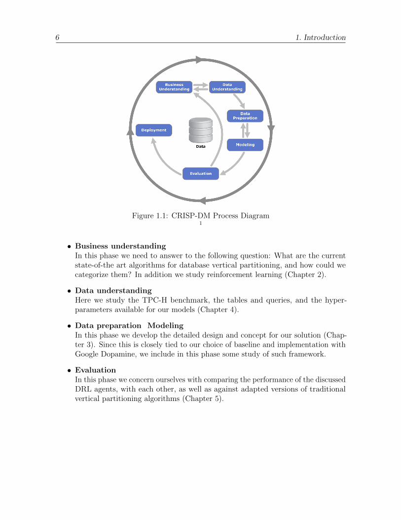
We follow the CRISP-DM [Wir00] process model as our research methodology. Thismethod is mainly applied for data mining projects and has already become standardized.Though our project is not strictly a data mining project, we decided that due to thegenerality of CRISP-DM, it could be easily adopted to guide this study.
Below we detail the phases of CRISP-DM (Figure 1.1), as we adopt them for ourresearch.
1https://en.wikipedia.org/wiki/Cross-industry standard process for data mining
6 1. Introduction
Figure 1.1: CRISP-DM Process Diagram1
• Business understandingIn this phase we need to answer to the following question: What are the currentstate-of-the art algorithms for database vertical partitioning, and how could wecategorize them? In addition we study reinforcement learning (Chapter 2).
• Data understandingHere we study the TPC-H benchmark, the tables and queries, and the hyper-parameters available for our models (Chapter 4).
• Data preparation ModelingIn this phase we develop the detailed design and concept for our solution (Chap-ter 3). Since this is closely tied to our choice of baseline and implementation withGoogle Dopamine, we include in this phase some study of such framework.
• EvaluationIn this phase we concern ourselves with comparing the performance of the discussedDRL agents, with each other, as well as against adapted versions of traditionalvertical partitioning algorithms (Chapter 5).
1.4. Thesis structure 7
1.4 Thesis structure
The rest of the thesis is structured as follows:
• In Chapter 2 we give document some necessary background information. Mainly,we discuss traditional approaches to database vertical partitioning, and we establishthe basic necessary RL and DRL concepts.
• In Chapter 3 we present the detailed design of our solution, describing the obser-vation space, the action space and semantics of actions and the rewarding schemewe designed. Since the design is closely related to some implementation aspects, inthis chapter we also introduce the Google Dopamine framework, and our choicesin selecting vertical partitioning algorithms as baselines.
• In Chapter 4 we introduce the precise research questions that will be answered byour evaluation. We also describe the benchmarking data selected, the experimentalsetup for our study and some relevant implementation details.
• Chapter 5 is dedicated to our experiments using different TPC-H tables, workloadsand hyper parameters. In this chapter we report and discuss our experimentalresults, answering to our research questions.
• In Chapter 6 we discuss related work in applying reinforcement learning methods fordifferent kind of database problems, providing a better context to understand ourresearch results and the outlook of our work. For keeping a cohesive presentationof our work, we place the majority of our studies on database self-driving tasks inthis section.
• In Chapter 7 we conclude this thesis and give the further directions for futureresearch.

8 1. Introduction
2. Background
In this chapter, we present a brief overview of the theoretical background and state ofthe art relevant to this thesis. We organize this chapter as follows:
• Horizontal and vertical partitioning:We start by describing the general goal and workings of partitioning approaches(Section 2.1).
• Vertical partition optimization algorithms:We follow by describing in detail four chosen vertical partitioning algorithms. Thisis important since these algorithms are the state of the art, and they represent thebaseline for evaluating our DRL-based solutions (Section 2.2).
• Reinforcement Learning:Next, we discuss the fundamental ideas behind reinforcement learning and deepreinforcement learning methods, as they are relevant to our research (Section 2.3).
• SummaryWe conclude this chapter by summarizing our studies (Section 2.4).
2.1 Horizontal and vertical partitioning
One central problem in database physical performance optimization is that of dividingan existing logical relation into optimally-defined physical partitions. The main purposeof this operation is to reduce I/O related costs, by keeping in memory only data that isrelevant to an expected workload.
There are several partitioning strategies, but the two basic ones for relational data arehorizontal and vertical partitioning [NCWD84a]. Horizontal partitioning is the processof dividing a relation into a set of tuples, called fragments, where each fragment has the
10 2. Background
same attributes as the original relation [NCWD84a]. Here each tuple must belong toat least one of the fragments defined, such that we are able to reconstruct the originalrelation after its partitioning [KS86].
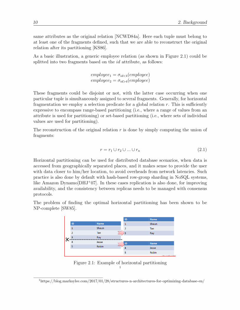
As a basic illustration, a generic employee relation (as shown in Figure 2.1) could besplitted into two fragments based on the id attribute, as follows:
employee1 = σid<4(employee)employee2 = σid>4(employee)
These fragments could be disjoint or not, with the latter case occurring when oneparticular tuple is simultaneously assigned to several fragments. Generally, for horizontalfragmentation we employ a selection predicate for a global relation r. This is sufficientlyexpressive to encompass range-based partitioning (i.e., where a range of values from anattribute is used for partitioning) or set-based partitioning (i.e., where sets of individualvalues are used for partitioning).
The reconstruction of the original relation r is done by simply computing the union offragments:
r = r1 ∪ r2 ∪ ... ∪ rn (2.1)
Horizontal partitioning can be used for distributed database scenarios, when data isaccessed from geographically separated places, and it makes sense to provide the userwith data closer to him/her location, to avoid overheads from network latencies. Suchpractice is also done by default with hash-based row-group sharding in NoSQL systems,like Amazon Dynamo[DHJ+07]. In these cases replication is also done, for improvingavailability, and the consistency between replicas needs to be managed with consensusprotocols.
The problem of finding the optimal horizontal partitioning has been shown to beNP-complete [SW85].
Figure 2.1: Example of horizontal partitioning1
1https://blog.marksylee.com/2017/01/28/structures-n-architectures-for-optimizing-database-en/
2.2. Vertical partitioning algorithms 11
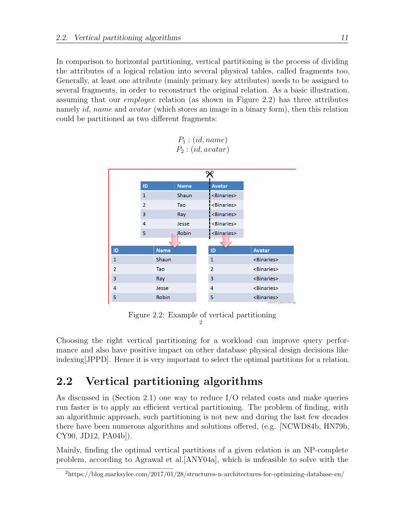
In comparison to horizontal partitioning, vertical partitioning is the process of dividingthe attributes of a logical relation into several physical tables, called fragments too.Generally, at least one attribute (mainly primary key attributes) needs to be assigned toseveral fragments, in order to reconstruct the original relation. As a basic illustration,assuming that our employee relation (as shown in Figure 2.2) has three attributesnamely id, name and avatar (which stores an image in a binary form), then this relationcould be partitioned as two different fragments:
P1 : (id, name)P2 : (id, avatar)
Figure 2.2: Example of vertical partitioning2
Choosing the right vertical partitioning for a workload can improve query perfor-mance and also have positive impact on other database physical design decisions likeindexing[JPPD]. Hence it is very important to select the optimal partitions for a relation.
2.2 Vertical partitioning algorithms
As discussed in (Section 2.1) one way to reduce I/O related costs and make queriesrun faster is to apply an efficient vertical partitioning. The problem of finding, withan algorithmic approach, such partitioning is not new and during the last few decadesthere have been numerous algorithms and solutions offered, (e.g. [NCWD84b, HN79b,CY90, JD12, PA04b]).
Mainly, finding the optimal vertical partitions of a given relation is an NP-completeproblem, according to Agrawal et al.[ANY04a], which is unfeasible to solve with the
2https://blog.marksylee.com/2017/01/28/structures-n-architectures-for-optimizing-database-en/
12 2. Background
optimal solution in a sub-exponential time, therefore is difficult to manage in case ofreal scenarios, without heuristics to reduce the search space[GCNG16, Ape88].
Therefore to find the best possible solution there have been algorithms proposed usingdifferent heuristics. One of the main problem here is that these algorithms mainlyare not universal solutions, and the selection of the proper algorithm must be donein consideration of different characteristics of the database like the database/queryprocessing paradigm, the hardware used, the workload specifications, among others.
The proposed vertical partitioning algorithms in the literature could be classified fromdifferent dimensions based the ideas behind them. Jindal et al. [JPPD] offered athree-dimensional classification:
• Search strategy
• Starting point
• Candidate Pruning
The first of these dimensions, search strategy, refers to how algorithms search the solutionspace. There are three main approaches: brute force, top-down and bottom-up:
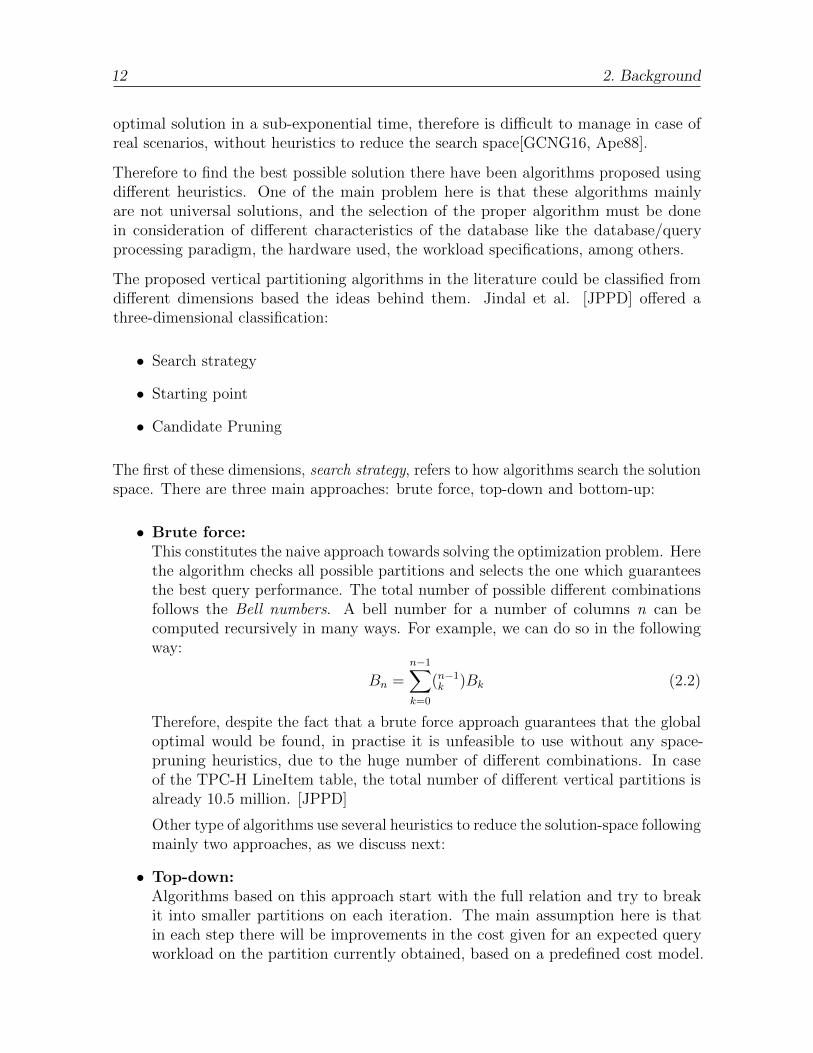
• Brute force:This constitutes the naive approach towards solving the optimization problem. Herethe algorithm checks all possible partitions and selects the one which guaranteesthe best query performance. The total number of possible different combinationsfollows the Bell numbers. A bell number for a number of columns n can becomputed recursively in many ways. For example, we can do so in the followingway:
Bn =n−1∑k=0
(n−1k )Bk (2.2)
Therefore, despite the fact that a brute force approach guarantees that the globaloptimal would be found, in practise it is unfeasible to use without any space-pruning heuristics, due to the huge number of different combinations. In caseof the TPC-H LineItem table, the total number of different vertical partitions isalready 10.5 million. [JPPD]
Other type of algorithms use several heuristics to reduce the solution-space followingmainly two approaches, as we discuss next:
• Top-down:Algorithms based on this approach start with the full relation and try to breakit into smaller partitions on each iteration. The main assumption here is thatin each step there will be improvements in the cost given for an expected queryworkload on the partition currently obtained, based on a predefined cost model.
2.2. Vertical partitioning algorithms 13
Algorithms stop the partitioning process when there are no longer improvementsin subsequent iterations. The earliest vertical partitioning algorithms followed thisapproach. [NCWD84a, NCWD84b] The ideas of this approach is also used forrecent algorithms proposed for an online environment [JD12, JQRD11]. Algorithmswith this approach are more suitable when the queries in the workload accessmainly the same attributes, since this might mean that the algorithm starts froma solution that is close to the optima.
• Bottom-up:In comparison to the former approach, these type of algorithms start with individualattributes as partitions, and recursively merge them at each iteration. This processcontinues until there are no longer improvements in query costs. The majorityof state-of-the art algorithms follow this approach [HP03, PA04a]. This type ofalgorithms are mainly suitable, and have advantages over top down solutions whenthe attributes show a highly-fragmented access pattern (i.e., this too might meanthat the algorithm starts from a solution that is close to the optima).
The second dimension to classify the vertical partitioning algorithms, is the startingpoint. This refers to whether the algorithm carries out some data pre-processing thatwould reduce the attribute set or the workload, that is fed into the partitioning solution.
Considering this dimension, some algorithms (e.g., Navathe [NCWD84a], O2P [JD12],Brute Force) start from the whole workload (i.e., considering all queries and attributesat the start). Algorithms like AutoPart [PA04b] and HillClimb [HP03] ) extract subsetsof the attribute space, choosing as a starting point a configuration where the originalattributes are sub-divided into groups using a k-way partitioner, and then letting thepartitioner compute vertical partitioning in each group. All sub-partitions are nextcombined for generating the complete solution. Attribute subset solutions decrease thecomplexity of the partitioning problem but the generated final solution could remainstuck in local optimas. The third type of selection takes as starting point a subset ofthe query space (or workload). This approach is relatively recent, and is based on querysimilarities inside a workload.This approach is used in Trojan [JQRD11].
The third classification dimension is candidate pruning. According to [JQRD11], ac-cording to [JQRD11] all algorithms except Trojan, do not apply any candidate pruningtechnique (save for the iterative computation) and only Trojan used a so-called threshold-based tuning in order to reduce the search space.
In our experiments we evaluate brute force, next to the Navathe, O2P, AutoPart andHillClimb algorithms, as baselines to provide an evaluation context for our DRL models.Given this choice, we consider that it is important to review these algorithms in detail,highlighting commonalities and differences between them. To conclude this section wesummarize some aspects about these algorithms. In the next section we discuss each ofthem (except brute force) in detail.
In Table 2.1 we classify the given algorithms based on the different dimensions discussed.In the following, Table 2.2, we report further details from the original implementations.
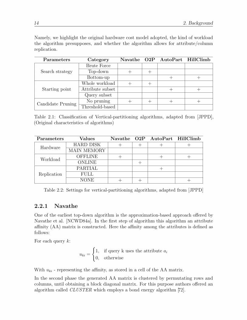
14 2. Background
Namely, we highlight the original hardware cost model adopted, the kind of workloadthe algorithm presupposes, and whether the algorithm allows for attribute/columnreplication.
Parameters Category Navathe O2P AutoPart HillClimb
Search strategyBrute ForceTop-down + +Bottom-up + +
Starting pointWhole workload + +Attribute subset + +
Query subset
Candidate PruningNo pruning + + + +
Threshold-based
Table 2.1: Classification of Vertical-partitioning algorithms, adapted from [JPPD],(Original characteristics of algorithms)
Parameters Values Navathe O2P AutoPart HillClimb
HardwareHARD DISK + + + +
MAIN MEMORY
WorkloadOFFLINE + + +ONLINE +
ReplicationPARTIAL +
FULLNONE + + +
Table 2.2: Settings for vertical-partitioning algorithms, adapted from [JPPD]
2.2.1 Navathe
One of the earliest top-down algorithm is the approximation-based approach offered byNavathe et al. [NCWD84a]. In the first step of algorithm this algorithm an attributeaffinity (AA) matrix is constructed. Here the affinity among the attributes is defined asfollows:
For each query k:
uki =
{1, if query k uses the attribute ai
0, otherwise
With uki - representing the affinity, as stored in a cell of the AA matrix.
In the second phase the generated AA matrix is clustered by permutating rows andcolumns, until obtaining a block diagonal matrix. For this purpose authors offered analgorithm called CLUSTER which employs a bond energy algorithm [72].
2.2. Vertical partitioning algorithms 15
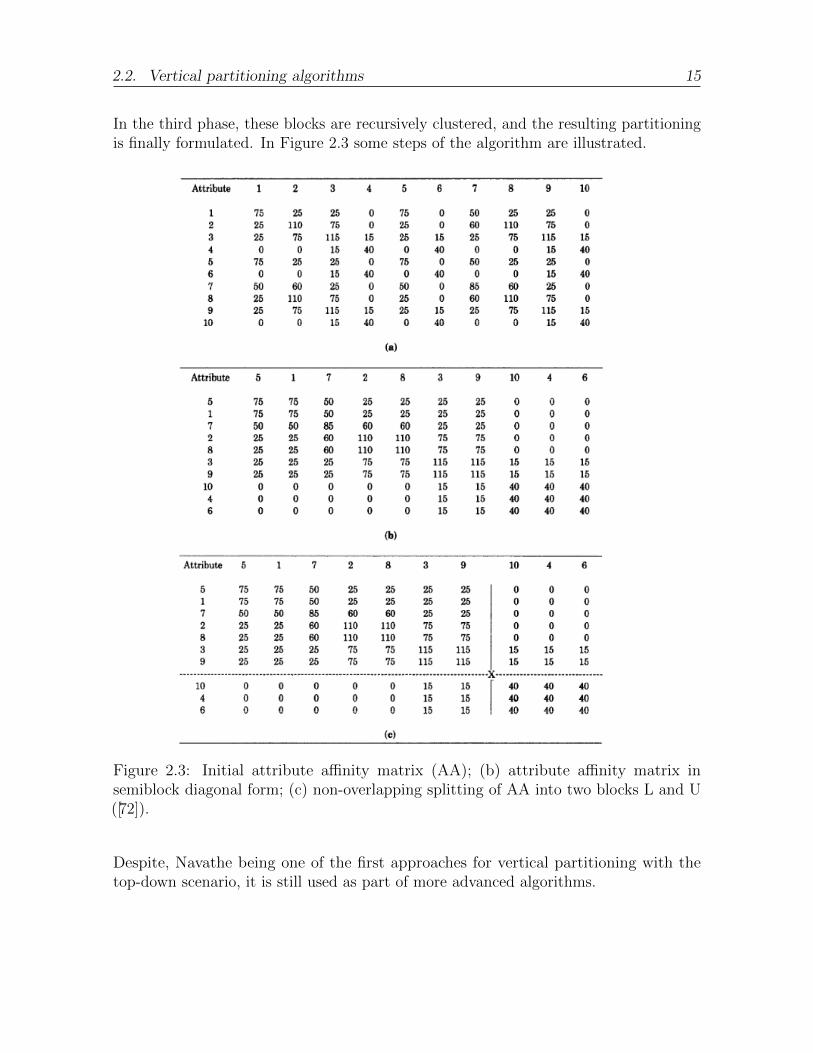
In the third phase, these blocks are recursively clustered, and the resulting partitioningis finally formulated. In Figure 2.3 some steps of the algorithm are illustrated.
Figure 2.3: Initial attribute affinity matrix (AA); (b) attribute affinity matrix insemiblock diagonal form; (c) non-overlapping splitting of AA into two blocks L and U([72]).
Despite, Navathe being one of the first approaches for vertical partitioning with thetop-down scenario, it is still used as part of more advanced algorithms.
16 2. Background
2.2.2 O2P
Recently another top down algorithm was offered by Jindal et.al [JD12], being mainlydesigned for an online environment. Authors suggest that the main disadvantages of theexisting vertical partitioning algorithms is that they are mainly offline solutions. So thereare problems when the workload is changing during the time. This is especially importantif there is concept drift (or rapidly changing workloads). In such cases it becomes difficultfor database administrator to adopt the recommendations from partitioning algorithmsappropriately. The offered solution AUTOSTORE works in an online environment,dynamically monitoring query workloads and dynamically clustering the partitions usinginterval-based analysis over the affinity matrix. For analyzing the partitions, the authorsoffered an online algorithm O2P which employs a greedy solution. Therefore, despitethe partitions generated by O2P being non-optimal ones, in practise they show decentand comparable results to other algorithms.
As described, O2P employs Navathe’s algorithm and dynamically updates the affinitymatrix for every incoming query. Dynamic programming is using for keeping the optimalsplit lines from previous steps.
This algorithm works by defining a partitioning unit, which corresponds to the smallestindivisible unit of storage (e.g. attribute groups that are always mentioned together onall queries). Next it defines an ordering inside each unit (i.e., the order of attributes inthe attribute affinity matrix, to help the block-wise clustering). Based on this order asplit vector S can be proposed, which defines with 0 if a given attribute is placed nextto the former one, or with 1 if there is a split. O2P does one dimensional partitioning,because it considers only one split line at a time. Finally, partitions are then defined bysplit lines, partitioning units and the corresponding orders.
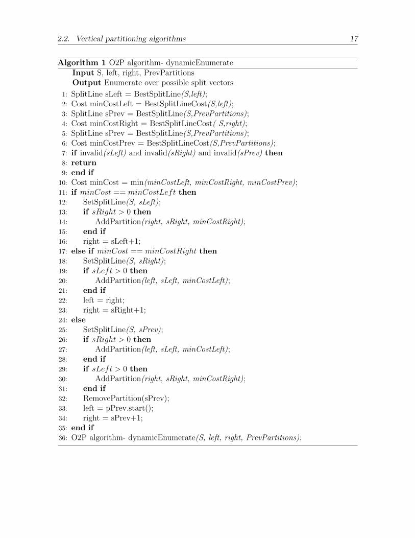
In 1 the pseudocode of O2P is shown. As mentioned, the call to O2P is recursive, takingas input the previous split vector (S), and information from previously evaluated splitlines in the left and right groups. It also takes as input the best in all previous partitions(PrevPartions). As mentioned, the algorithm reuses or computes the informationregarding the best split line found in all previous partition, and the minimum cost forthe best split in the two groups along the current split vector (lines 1-6). The algorithmstops if one split line is invalid (lines 7-8). Next it evaluates the minimum cost obtainedfor the three lines (line 10), and chooses the one having the minimum cost, setting thenext parameters such that computation can be reused (lines 11-35).
2.2. Vertical partitioning algorithms 17
Algorithm 1 O2P algorithm- dynamicEnumerateInput S, left, right, PrevPartitionsOutput Enumerate over possible split vectors
1: SplitLine sLeft = BestSplitLine(S,left);2: Cost minCostLeft = BestSplitLineCost(S,left);3: SplitLine sPrev = BestSplitLine(S,PrevPartitions);4: Cost minCostRight = BestSplitLineCost( S,right);5: SplitLine sPrev = BestSplitLine(S,PrevPartitions);6: Cost minCostPrev = BestSplitLineCost(S,PrevPartitions);7: if invalid(sLeft) and invalid(sRight) and invalid(sPrev) then8: return9: end if10: Cost minCost = min(minCostLeft, minCostRight, minCostPrev);11: if minCost == minCostLeft then12: SetSplitLine(S, sLeft);13: if sRight > 0 then14: AddPartition(right, sRight, minCostRight);15: end if16: right = sLeft+1;17: else if minCost == minCostRight then18: SetSplitLine(S, sRight);19: if sLeft > 0 then20: AddPartition(left, sLeft, minCostLeft);21: end if22: left = right;23: right = sRight+1;24: else25: SetSplitLine(S, sPrev);26: if sRight > 0 then27: AddPartition(left, sLeft, minCostLeft);28: end if29: if sLeft > 0 then30: AddPartition(right, sRight, minCostRight);31: end if32: RemovePartition(sPrev);33: left = pPrev.start();34: right = sPrev+1;35: end if36: O2P algorithm- dynamicEnumerate(S, left, right, PrevPartitions);
18 2. Background
2.2.3 AutoPart
Papadomanolakis et al. offered a bottom-up algorithm called AutoPart [PA04b].
Authors offered two types of fragments:
1. Atomic - the thinnest possible fragment of a given relation, which are accessedatomically (i.e there is no query which access the subset of atomic fragment)
2. Composite - union of several atomic fragments
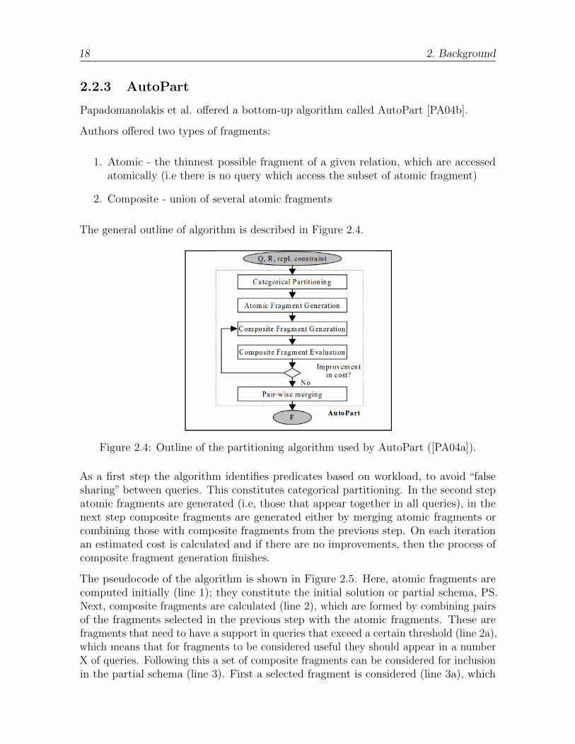
The general outline of algorithm is described in Figure 2.4.
Figure 2.4: Outline of the partitioning algorithm used by AutoPart ([PA04a]).
As a first step the algorithm identifies predicates based on workload, to avoid “falsesharing” between queries. This constitutes categorical partitioning. In the second stepatomic fragments are generated (i.e, those that appear together in all queries), in thenext step composite fragments are generated either by merging atomic fragments orcombining those with composite fragments from the previous step. On each iterationan estimated cost is calculated and if there are no improvements, then the process ofcomposite fragment generation finishes.
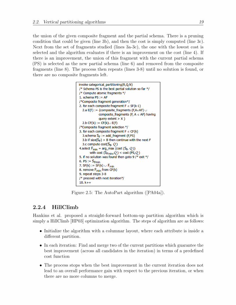
The pseudocode of the algorithm is shown in Figure 2.5. Here, atomic fragments arecomputed initially (line 1); they constitute the initial solution or partial schema, PS.Next, composite fragments are calculated (line 2), which are formed by combining pairsof the fragments selected in the previous step with the atomic fragments. These arefragments that need to have a support in queries that exceed a certain threshold (line 2a),which means that for fragments to be considered useful they should appear in a numberX of queries. Following this a set of composite fragments can be considered for inclusionin the partial schema (line 3). First a selected fragment is considered (line 3a), which
2.2. Vertical partitioning algorithms 19
the union of the given composite fragment and the partial schema. There is a pruningcondition that could be given (line 3b), and then the cost is simply computed (line 3c).Next from the set of fragments studied (lines 3a-3c), the one with the lowest cost isselected and the algorithm evaluates if there is an improvement on the cost (line 4). Ifthere is an improvement, the union of this fragment with the current partial schema(PS) is selected as the new partial schema (line 6) and removed from the compositefragments (line 8). The process then repeats (lines 3-8) until no solution is found, orthere are no composite fragments left.
Figure 2.5: The AutoPart algorithm ([PA04a]).
2.2.4 HillClimb
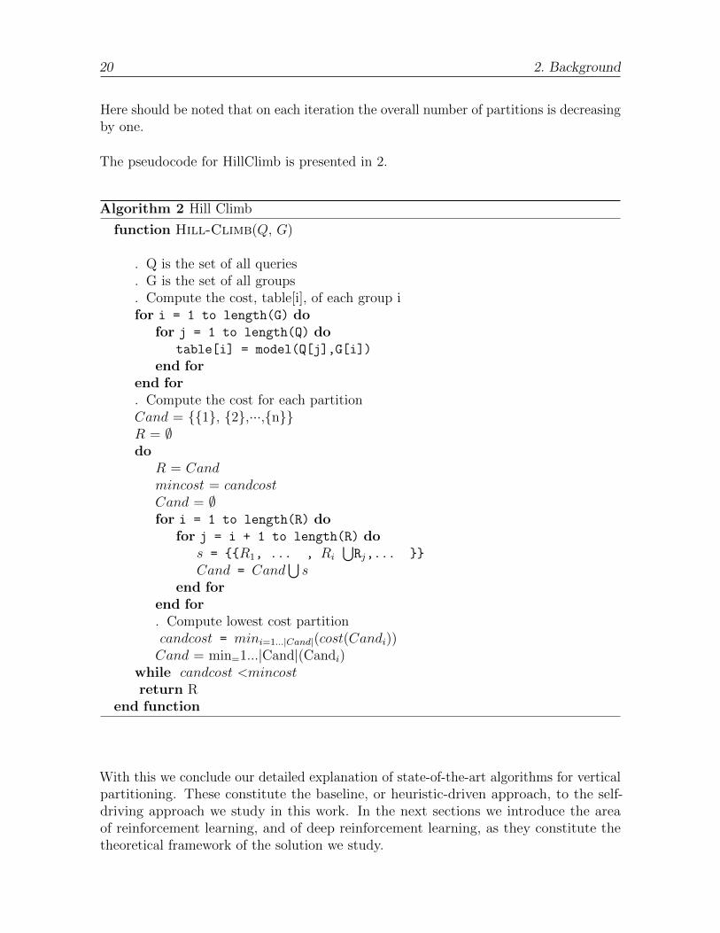
Hankins et al. proposed a straight-forward bottom-up partition algorithm which issimply a HillClimb [HP03] optimization algorithm. The steps of algorithm are as follows:
• Initialize the algorithm with a columnar layout, where each attribute is inside adifferent partition.
• In each iteration: Find and merge two of the current partitions which guarantee thebest improvement (across all candidates in the iteration) in terms of a predefinedcost function
• The process stops when the best improvement in the current iteration does notlead to an overall performance gain with respect to the previous iteration, or whenthere are no more columns to merge.
20 2. Background
Here should be noted that on each iteration the overall number of partitions is decreasingby one.
The pseudocode for HillClimb is presented in 2.
Algorithm 2 Hill Climb
function Hill-Climb(Q, G)
. Q is the set of all queries
. G is the set of all groups
. Compute the cost, table[i], of each group ifor i = 1 to length(G) do
for j = 1 to length(Q) dotable[i] = model(Q[j],G[i])
end forend for. Compute the cost for each partitionCand = {{1}, {2},···,{n}}R = ∅do
R = Candmincost = candcostCand = ∅for i = 1 to length(R) do
for j = i + 1 to length(R) dos = {{R1, ... , Ri
⋃Rj,... }}
Cand = Cand⋃s
end forend for. Compute lowest cost partitioncandcost = mini=1...|Cand|(cost(Candi))Cand = min=1...|Cand|(Candi)
while candcost <mincostreturn R
end function
With this we conclude our detailed explanation of state-of-the-art algorithms for verticalpartitioning. These constitute the baseline, or heuristic-driven approach, to the self-driving approach we study in this work. In the next sections we introduce the areaof reinforcement learning, and of deep reinforcement learning, as they constitute thetheoretical framework of the solution we study.
2.3. Reinforcement learning 21
2.3 Reinforcement learning
In this section we briefly discuss reinforcement learning (RL). Since, the topic is verybroad we decide to focus only on the essential concepts relevant to our current research.
We structure this section as follows:
• We start by discussing general reinforcement learning, introducing the basicterminology (Section 2.3.1).
• Subsequently we discuss Deep Q-learning (DQN) based approaches, since they area state-of-the art family of approaches in deep RL algorithms, and we use modelsbased on these approaches for our study (Section 2.3.2).
2.3.1 RL basics
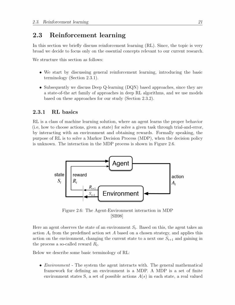
RL is a class of machine learning solution, where an agent learns the proper behavior(i.e, how to choose actions, given a state) for solve a given task through trial-and-error,by interacting with an environment and obtaining rewards. Formally speaking, thepurpose of RL is to solve a Markov Decision Process (MDP), when the decision policyis unknown. The interaction in the MDP process is shown in Figure 2.6.
Figure 2.6: The Agent-Environment interaction in MDP[SB98]
Here an agent observes the state of an environment St. Based on this, the agent takes anaction At from the predefined action set A based on a chosen strategy, and applies thisaction on the environment, changing the current state to a next one St+1 and gaining inthe process a so-called reward Rt.
Below we describe some basic terminology of RL:
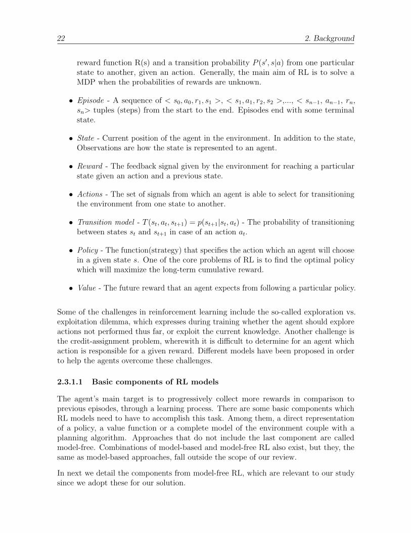
• Environment - The system the agent interacts with. The general mathematicalframework for defining an environment is a MDP. A MDP is a set of finiteenvironment states S, a set of possible actions A(s) in each state, a real valued
22 2. Background
reward function R(s) and a transition probability P (s′, s|a) from one particularstate to another, given an action. Generally, the main aim of RL is to solve aMDP when the probabilities of rewards are unknown.
• Episode - A sequence of < s0, a0, r1, s1 >, < s1, a1, r2, s2 >,..., < sn−1, an−1, rn,sn> tuples (steps) from the start to the end. Episodes end with some terminalstate.
• State - Current position of the agent in the environment. In addition to the state,Observations are how the state is represented to an agent.
• Reward - The feedback signal given by the environment for reaching a particularstate given an action and a previous state.
• Actions - The set of signals from which an agent is able to select for transitioningthe environment from one state to another.
• Transition model - T (st, at, st+1) = p(st+1|st, at) - The probability of transitioningbetween states st and st+1 in case of an action at.
• Policy - The function(strategy) that specifies the action which an agent will choosein a given state s. One of the core problems of RL is to find the optimal policywhich will maximize the long-term cumulative reward.
• Value - The future reward that an agent expects from following a particular policy.
Some of the challenges in reinforcement learning include the so-called exploration vs.exploitation dilemma, which expresses during training whether the agent should exploreactions not performed thus far, or exploit the current knowledge. Another challenge isthe credit-assignment problem, wherewith it is difficult to determine for an agent whichaction is responsible for a given reward. Different models have been proposed in orderto help the agents overcome these challenges.
2.3.1.1 Basic components of RL models
The agent’s main target is to progressively collect more rewards in comparison toprevious episodes, through a learning process. There are some basic components whichRL models need to have to accomplish this task. Among them, a direct representationof a policy, a value function or a complete model of the environment couple with aplanning algorithm. Approaches that do not include the last component are calledmodel-free. Combinations of model-based and model-free RL also exist, but they, thesame as model-based approaches, fall outside the scope of our review.
In next we detail the components from model-free RL, which are relevant to our studysince we adopt these for our solution.
2.3. Reinforcement learning 23
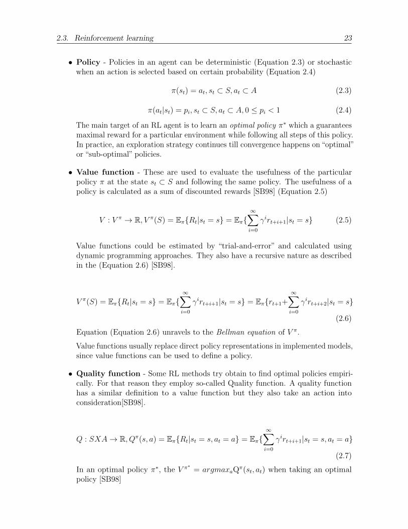
• Policy - Policies in an agent can be deterministic (Equation 2.3) or stochasticwhen an action is selected based on certain probability (Equation 2.4)
π(st) = at, st ⊂ S, at ⊂ A (2.3)
π(at|st) = pi, st ⊂ S, at ⊂ A, 0 ≤ pi < 1 (2.4)
The main target of an RL agent is to learn an optimal policy π∗ which a guaranteesmaximal reward for a particular environment while following all steps of this policy.In practice, an exploration strategy continues till convergence happens on “optimal”or “sub-optimal” policies.
• Value function - These are used to evaluate the usefulness of the particularpolicy π at the state st ⊂ S and following the same policy. The usefulness of apolicy is calculated as a sum of discounted rewards [SB98] (Equation 2.5)
V : V π → R, V π(S) = Eπ{Rt|st = s} = Eπ{∞∑i=0
γirt+i+1|st = s} (2.5)
Value functions could be estimated by “trial-and-error” and calculated usingdynamic programming approaches. They also have a recursive nature as describedin the (Equation 2.6) [SB98].
V π(S) = Eπ{Rt|st = s} = Eπ{∞∑i=0
γirt+i+1|st = s} = Eπ{rt+1+∞∑i=0
γirt+i+2|st = s}
(2.6)
Equation (Equation 2.6) unravels to the Bellman equation of V π.
Value functions usually replace direct policy representations in implemented models,since value functions can be used to define a policy.
• Quality function - Some RL methods try obtain to find optimal policies empiri-cally. For that reason they employ so-called Quality function. A quality functionhas a similar definition to a value function but they also take an action intoconsideration[SB98].
Q : SXA→ R, Qπ(s, a) = Eπ{Rt|st = s, at = a} = Eπ{∞∑i=0
γirt+i+1|st = s, at = a}
(2.7)
In an optimal policy π∗, the V π∗ = argmaxaQπ(st, at) when taking an optimal
policy [SB98]
24 2. Background
2.3.1.2 Q-learning and SARSA
The idea of temporal-difference learning (TD) [SB98] is based on dynamic programming(DP) and is related to Monte Carlo methods. In comparison to Monte Carlo methodswhere the entire episode needs to finished to able to be able to update the value function,TD-learning is able to learn value function within each step. In comparison to DP wherethe model of the environment’s dynamic is necessary, TD is suitable for uncertain andunpredictable tasks. There are two possible algorithms offered for TD-learning tasks.
• off-policy Q-learning algorithm offered by Watkins et al [WD92]
• on-policy SARSA algorithm offered by Sutton et al [SB98]
For updating the action-value-function on-policy methods update the value given for thecurrent action by considering the future actions based on the current policy, whereas off-policy methods use policies different that the current one for calculating the discountedreward (i.e., the next action) for a given action-value-function.
Q-learning is an off-policy algorithm because to approximate optimal Q-value functionQ∗ it does not consider the current policy. The update step is described in Equation 2.8.
Q(st, at)← Q(st, at) + α(rt+1 + γmaxaQ(st+1, at+1)−Q(st, at)) (2.8)
Here α is a learning rate (0<α ≤1) that determines how fast the old Q-value will beupdated based on new experiences. γ is a discount factor that is used to balance howmuch the value of future states will impact the value of the current state.
It has been proven that Q-learning converges to the optimal provided that the state-action pairs are represented discretely, and that during exploration all actions arerepeatedly sampled in all states (which, as authors point out [FLHI+18], ensures sufficientexploration)[WD92].
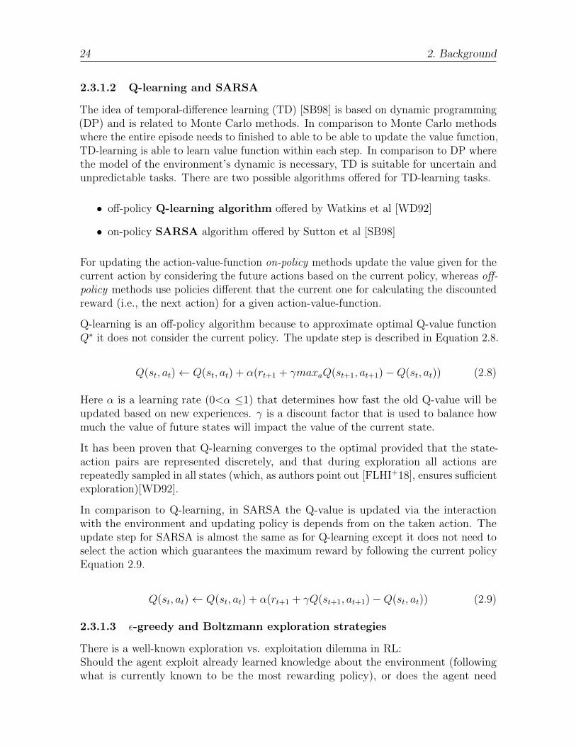
In comparison to Q-learning, in SARSA the Q-value is updated via the interactionwith the environment and updating policy is depends from on the taken action. Theupdate step for SARSA is almost the same as for Q-learning except it does not need toselect the action which guarantees the maximum reward by following the current policyEquation 2.9.
Q(st, at)← Q(st, at) + α(rt+1 + γQ(st+1, at+1)−Q(st, at)) (2.9)
2.3.1.3 ε-greedy and Boltzmann exploration strategies
There is a well-known exploration vs. exploitation dilemma in RL:Should the agent exploit already learned knowledge about the environment (followingwhat is currently known to be the most rewarding policy), or does the agent need
2.3. Reinforcement learning 25
to explore more unknown states to be able to find a better policy? Obviously, atthe beginning of its training the agent should explore larger amount of states, andthen he could exploit the gathered knowledge till he is confident enough of the results.The problem here is finding the right trade-off for how to switch between explorationand exploitation, and this could be hard to achieve in the case of uncertain/dynamicenvironments.
There are several methods proposed for managing this challenge:
• ε - greedy strategy: In this series of strategies, given the Q-function Q(s, a) anagent randomly selects a action based on predefined ε - probability ( 0 ≤ ε < 1) and selects the best action which maximizes the Q-value for a given state in(1- ε) cases. In most cases, it is better to select a high ε at the beginning of thetask and decrease it gradually as the training increases (decrease exploration overexploitation). This is the idea of decaying ε - greedy approaches, where a varietyof functions could be used to decrease ε over time.
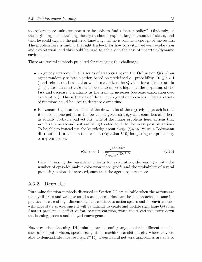
• Boltzmann Exploration - One of the drawbacks of the ε-greedy approach is thatit considers one action as the best for a given strategy and considers all othersas equally probable bad actions. One of the major problems here, actions thatwould rank as second best are being treated equal to the worst possible actions.To be able to instead use the knowledge about every Q(st, at) value, a Boltzmanndistribution is used as in the formula (Equation 2.10) for getting the probabilityof a given action:
p(at|st, Qt) =eQ(st,at)/τ∑b⊂AS
eQ(st,b)/τ(2.10)
Here increasing the parameter τ leads for exploration, decreasing τ with thenumber of episodes make exploration more greedy and the probability of severalpromising actions is increased, such that the agent explores more.
2.3.2 Deep RL
Pure value-function methods discussed in Section 2.3 are suitable when the actions aremainly discrete and we have small state spaces. However these approaches become im-practical in case of high-dimensional and continuous action spaces and for environmentswith huge state spaces, since it will be difficult to create and update such large Q-tables.Another problem is ineffective feature representation, which could lead to slowing downthe learning process and delayed convergence.
Nowadays, deep Learning (DL) solutions are becoming very popular in different domainssuch as computer vision, speech recognition, machine translation, etc. where they areable to demonstrate nice results[DY+14]. Deep neural network approaches are able to
26 2. Background
learn very complex features from raw input. Deep learning refers to the use of artificialneural networks for machine learning. Nowadays these models have become mainstreamthanks to developments in specialized kinds of neurons (e.g. convolutional, recurrent,GANs), optimization algorithms (e.g. Adam, Nesterov) and the standardization insupporting technologies, including libraries such as Caffe, Keras or Tensorflow-slim.
DL approaches show promising results too when combined with RL, being used forfunction approximation (i.e., such that the neural network maps between a state tothe Q-values predicted for the actions). The idea here is that it is overwhelming tostore each state in memory, specially if these states are very similar (in computer gamesthere could be only one single pixel difference between two sequential frames(states)).Therefore, instead of getting exact Q-values of a concrete state, we would involve deepneural networks to approximate Q-values (Equation 2.11). Here the parameters of theneural network (weights, biases, activation functions, etc., are represented as θ)
Q∗(st, at, θ) ≈ Q∗(st, at) (2.11)
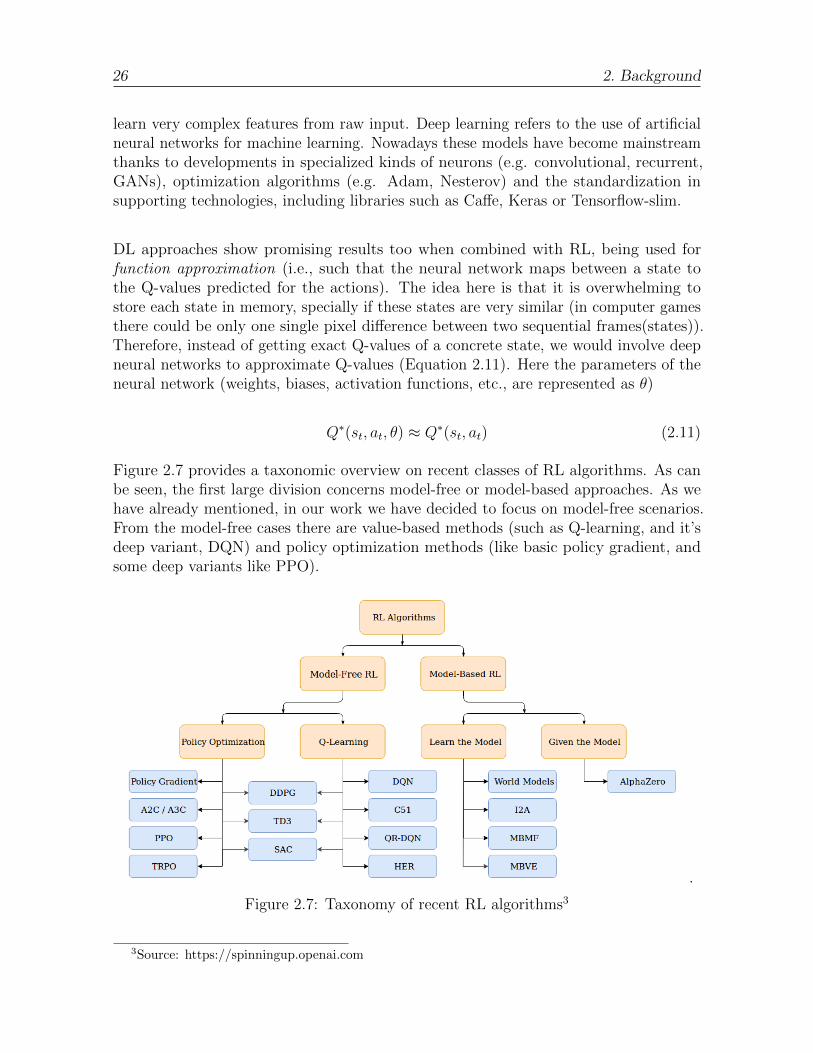
Figure 2.7 provides a taxonomic overview on recent classes of RL algorithms. As canbe seen, the first large division concerns model-free or model-based approaches. As wehave already mentioned, in our work we have decided to focus on model-free scenarios.From the model-free cases there are value-based methods (such as Q-learning, and it’sdeep variant, DQN) and policy optimization methods (like basic policy gradient, andsome deep variants like PPO).
.
Figure 2.7: Taxonomy of recent RL algorithms3
3Source: https://spinningup.openai.com
2.3. Reinforcement learning 27
In the further sections we provide a summarized overview of the DRL approach whichwe used for our models. In detail we review a subset of methods from the DQN class.
2.3.2.1 Deep Q-Network (DQN)
The deep Q-network (DQN), approach of applying deep reinforcement learning as offeredby Mnih et al. [MKS+13],[MKS+15] was able to successfully learn how to play various Atari Games.
In the original DQN algorithm, a neural network was added a substitute of Q-tables inQ-learning, and it as fed first pre-processed images from atari game emulators as aninput. A convolutional neural network (CNN) was employed. In this case the agent hadaccess only to a game’s score, which it considered as a reward.
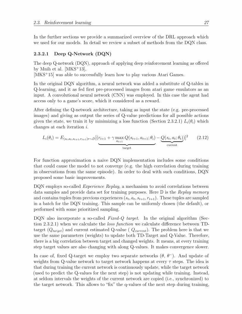
After defining the Q-network architecture, taking as input the state (e.g. pre-processedimages) and giving as output the series of Q-value predictions for all possible actionsgiven the state, we train it by minimizing a loss function (Section 2.3.2.1) Li(θi) whichchanges at each iteration i.
Li(θi) = E(st,at,st+1,rt+1)r∼D[(rt+1 + γmaxat+1
Q(st+1, at+1; θi)︸ ︷︷ ︸target
−Q(st, at; θt)︸ ︷︷ ︸current
)]2 (2.12)
For function approximation a naive DQN implementation includes some conditionsthat could cause the model to not converge (e.g. the high correlation during trainingin observations from the same episode). In order to deal with such conditions, DQNproposed some basic improvements.
DQN employs so-called Experience Replay, a mechanism to avoid correlations betweendata samples and provide data set for training purposes. Here D is the Replay memoryand contains tuples from previous experiences (st, at, st+1, rt+1). These tuples are sampledin a batch for the DQN training. This sample can be uniformly chosen (the default), orperformed with some prioritized sampling.
DQN also incorporate a so-called Fixed-Q target. In the original algorithm (Sec-tion 2.3.2.1) when we calculate the loss function we calculate difference between TD-target (Qtarget) and current estimated Q-value ( Qcurrent). The problem here is that weuse the same parameters (weights) to update both TD-Target and Q-Value. Therefore,there is a big correlation between target and changed weights. It means, at every trainingstep target values are also changing with along Q-values. It makes convergence slower.
In case of, fixed Q-target we employ two separate networks (θ, θ−). And update ofweights from Q-value network to target network happens at every τ steps. The idea isthat during training the current network is continuously update, while the target network(used to predict the Q-values for the next step) is not updating while training. Instead,at seldom intervals the weights of the current network are copied (i.e., synchronized) tothe target network. This allows to “fix” the q-values of the next step during training,
28 2. Background
such that the q-values being updated do not affect those predictions, and the trainingconverges better. This allows to have more stable learning due to target network stayfixed for a while. This is also shown in .
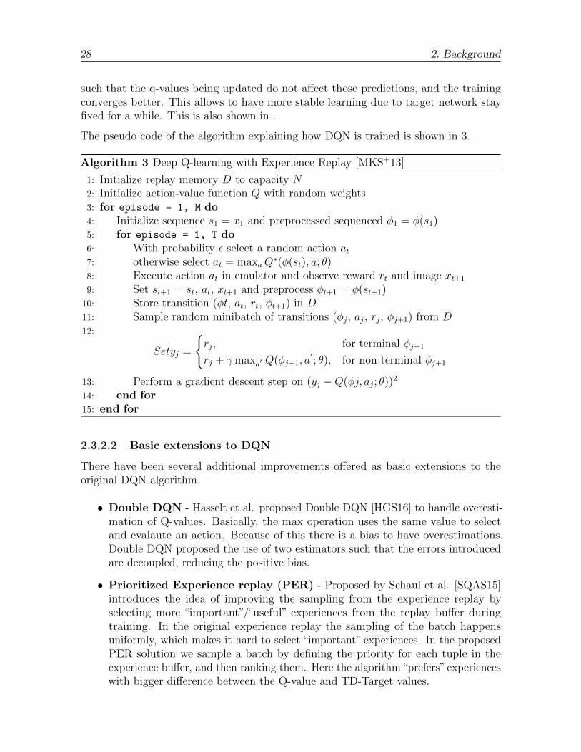
The pseudo code of the algorithm explaining how DQN is trained is shown in 3.
Algorithm 3 Deep Q-learning with Experience Replay [MKS+13]
1: Initialize replay memory D to capacity N2: Initialize action-value function Q with random weights3: for episode = 1, M do4: Initialize sequence s1 = x1 and preprocessed sequenced φ1 = φ(s1)5: for episode = 1, T do6: With probability ε select a random action at7: otherwise select at = maxaQ
∗(φ(st), a; θ)8: Execute action at in emulator and observe reward rt and image xt+1
9: Set st+1 = st, at, xt+1 and preprocess φt+1 = φ(st+1)10: Store transition (φt, at, rt, φt+1) in D11: Sample random minibatch of transitions (φj, aj, rj, φj+1) from D12:
Setyj =
{rj, for terminal φj+1
rj + γmaxa′ Q(φj+1, a′; θ), for non-terminal φj+1
13: Perform a gradient descent step on (yj −Q(φj, aj; θ))2
14: end for15: end for
2.3.2.2 Basic extensions to DQN
There have been several additional improvements offered as basic extensions to theoriginal DQN algorithm.
• Double DQN - Hasselt et al. proposed Double DQN [HGS16] to handle overesti-mation of Q-values. Basically, the max operation uses the same value to selectand evalaute an action. Because of this there is a bias to have overestimations.Double DQN proposed the use of two estimators such that the errors introducedare decoupled, reducing the positive bias.
• Prioritized Experience replay (PER) - Proposed by Schaul et al. [SQAS15]introduces the idea of improving the sampling from the experience replay byselecting more “important”/“useful” experiences from the replay buffer duringtraining. In the original experience replay the sampling of the batch happensuniformly, which makes it hard to select “important” experiences. In the proposedPER solution we sample a batch by defining the priority for each tuple in theexperience buffer, and then ranking them. Here the algorithm “prefers” experienceswith bigger difference between the Q-value and TD-Target values.
2.3. Reinforcement learning 29
More advanced extensions to DQN, affecting the neural network design have also beenproposed. We discuss two of them, as they correspond to models we use in our solution.
2.3.2.3 Distributional RL
In their work Bellemare et al. proposed an approach called Distributional RL, whichmainly learns to approximate the complete distribution rather than the approximateexpectation of each Q-value. [BDM17] In RL we use the Bellman equation for expectedvalue approximation. But in case of a stochastic environment choosing actions based onan expected value could be a reason for non-optimal solutions.In disributional RL we directly work with the full distribution of returns. Here we definea random variable Z(s, a) - starting from the state s, and performing action a for thecurrent policy. In that case we could define value-function in terms of a Z-function asshown in Equation 2.13.
Qπ(s, a) = E[Zπ(s, a)] (2.13)
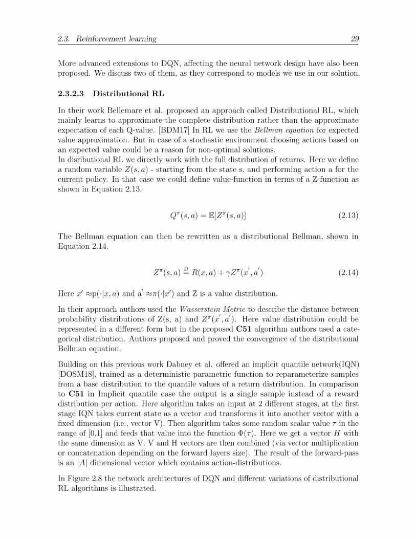
The Bellman equation can then be rewritten as a distributional Bellman, shown inEquation 2.14.
Zπ(s, a)D= R(x, a) + γZπ(x
′, a′) (2.14)
Here x′ ≈p(·|x, a) and a′ ≈π(·|x′) and Z is a value distribution.
In their approach authors used the Wasserstein Metric to describe the distance betweenprobability distributions of Z(s, a) and Zπ(x
′, a′). Here value distribution could be
represented in a different form but in the proposed C51 algorithm authors used a cate-gorical distribution. Authors proposed and proved the convergence of the distributionalBellman equation.
Building on this previous work Dabney et al. offered an implicit quantile network(IQN)[DOSM18], trained as a deterministic parametric function to reparameterize samplesfrom a base distribution to the quantile values of a return distribution. In comparisonto C51 in Implicit quantile case the output is a single sample instead of a rewarddistribution per action. Here algorithm takes an input at 2 different stages, at the firststage IQN takes current state as a vector and transforms it into another vector with afixed dimension (i.e., vector V). Then algorithm takes some random scalar value τ in therange of [0,1] and feeds that value into the function Φ(τ). Here we get a vector H withthe same dimension as V. V and H vectors are then combined (via vector multiplicationor concatenation depending on the forward layers size). The result of the forward-passis an |A| dimensional vector which contains action-distributions.
In Figure 2.8 the network architectures of DQN and different variations of distributionalRL algorithms is illustrated.
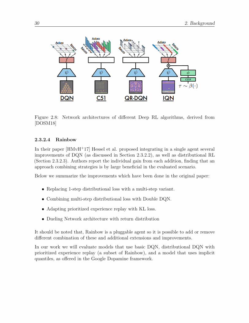
30 2. Background
Figure 2.8: Network architectures of different Deep RL algorithms, derived from[DOSM18]
2.3.2.4 Rainbow
In their paper [HMvH+17] Hessel et al. proposed integrating in a single agent severalimprovements of DQN (as discussed in Section 2.3.2.2), as well as distributional RL(Section 2.3.2.3). Authors report the individual gain from each addition, finding that anapproach combining strategies is by large beneficial in the evaluated scenario.
Below we summarize the improvements which have been done in the original paper:
• Replacing 1-step distributional loss with a multi-step variant.
• Combining multi-step distributional loss with Double DQN.
• Adapting prioritized experience replay with KL loss.
• Dueling Network architecture with return distribution
It should be noted that, Rainbow is a pluggable agent so it is possible to add or removedifferent combination of these and additional extensions and improvements.
In our work we will evaluate models that use basic DQN, distributional DQN withprioritized experience replay (a subset of Rainbow), and a model that uses implicitquantiles, as offered in the Google Dopamine framework.

2.4. Summary 31
2.4 Summary
In this chapter we discussed necessary background knowledge which we believe will behelpful to understand the next chapters of this thesis.
First we provided the core ideas behind partitioning approaches, and the reason whyDBMS systems need such optimization. We described different vertical partitioningalgorithms, categorized them based on different dimensions, and briefly described aselection of them.
Following this we discussed state-of-the art RL approaches, which we use for ourexperiments and evaluations.
In the next chapter, we describe the design of our solution.

32 2. Background
3. Self-driving vertical partitioningwith deep reinforcement learning
In this chapter we present the design for our solution. Our design is based on combiningtwo general aspects. First, the use of cost models and experts (i.e., traditional verticalpartitioning algorithms) playing a role in normalizing the rewards. Second, the designof the environment itself allowing, in combination with the agents, for an RL process.In this chapter we describe this in detail. We structure our description as follows:
Architecture of our solution:First, we establish the architecture or our solution, with all constitutent components(Section 3.1).
GridWorld environment:Second, we present the GridWorld environment, which encompasses all details pertainingto action space, action semantics, observation space and reward engineering (Section 3.2).
Summary:We conclude the chapter by summarizing the contents.
3.1 Architecture of our solution
Our implementation contains two separate parts:
1. To be able to learn and later to compare our proposed RL models with state-of-the art vertical partitioning algorithms. For this we use adapted versions ofthese algorithms proposed by [JPPD] and available as an open-source project1
1https://github.com/palatinuse/database-vertical-partitioning/
34 3. Self-driving vertical partitioning with deep reinforcement learning
implemented in the Java programming language. Since we use a form of learningfrom experts (in our case, we adopt the rewards of the experts to normalize therewarding scheme), we implemented REST APIs using the dropwizard framework2
which helped us to interact efficiently with these implementations.
2. The second part comprises the RL framework itself, including our own environment,which we implement as an OpenAI Gym environment3, such that it can be thencalled with state-of-the-art agents provided by the RL framework Google Dopamine4.
To implement our RL based approaches we selected Dopamine - a framework for easyprototyping RL algorithms. Dopamine makes it easy for benchmark experimentation,allows easily integrate our own environment and research ideas to the framework andprovide most state-of-the art proven algorithms out-of the box [CMG+18]. Dopamine inturn uses Tensorflow and Tensorflow-slim, for managing neural networks.
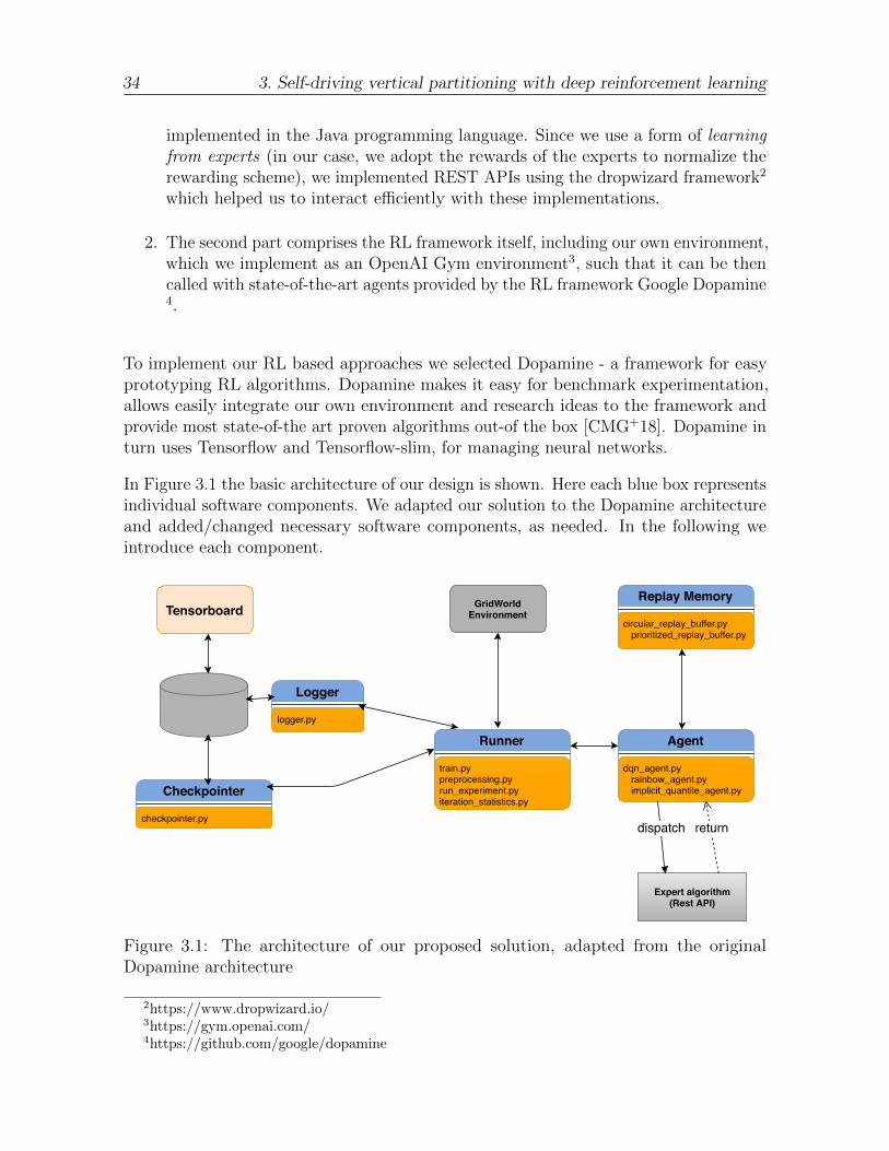
In Figure 3.1 the basic architecture of our design is shown. Here each blue box representsindividual software components. We adapted our solution to the Dopamine architectureand added/changed necessary software components, as needed. In the following weintroduce each component.
Tensorboard
Logger
logger.py
Checkpointer
checkpointer.py
GridWorldEnvironment
Runner
train.pypreprocessing.pyrun_experiment.pyiteration_statistics.py
Replay Memory
circular_replay_buffer.py prioritized_replay_buffer.py
Agent
dqn_agent.py rainbow_agent.py implicit_quantile_agent.py
Expert algorithm (Rest API)
dispatch return
Figure 3.1: The architecture of our proposed solution, adapted from the originalDopamine architecture
2https://www.dropwizard.io/3https://gym.openai.com/4https://github.com/google/dopamine
3.2. Grid World Environment 35
1. Runner - organizes the learning process, launching an experiment decomposedinto iterations, in turn composed of test and evaluate phases. The runner acts as amiddleware, initializing the environment, connecting agents with the environment,and providing agents with the states from environment for inference and learning.The runner also manages the logging.
2. Agents - A DQN family of models is provided out-of-the box (requiring onlyminimal changes to run with new environments) and their hyper parameters areeasily configurable using gin files. We had to adapt some agent behaviors for ouruse case (e.g. by introducing action pruning, or by adding novel parameters notavailable in Dopamine, like soft-updates).
3. Replay Memory - As described previously, the DQN family of algorithms usesa replay memory for effective learning. Dopamine provides several advancedimplementations of this. Almost no changes were required to adopt these.
4. GridWorld Environment - Our learning environment, encompassing the ma-jority of our choices for modeling vertical partitioning as a DRL task. We discussit in detail in Section 3.2.
5. Logger - This component is used for saving experiment statistics for furthervisualization and plot analysis, using Colab or Tensorboard.
6. Checkpointer - For long running experiments a checkpointer component isprovided that allows to periodically save the experiment states for weight re-uselater on.
7. Experts - We require to compare with experts, as a baseline. Four our work wepropose that the expertise of existing solutions can also be used. We discuss thisin detail in Section 3.2.
3.2 Grid World Environment
Below we describe the main characteristics of our environment. We called our environ-ment Grid World
Actions - We consider a learning environment with discrete actions. In our implemen-tation we follow a “bottom-up” approach. At the beginning of each episode we considereach attribute as separated partitions. At each step we do only one action and mergetwo available partitions.
Since our experiments are based on the TPC-H benchmark and the largest relation onthis benchmark (LINEITEM) contains 16 attributes the overall action set contains thefollowing number of actions: (
16
2
)= 120
36 3. Self-driving vertical partitioning with deep reinforcement learning
.
As an example for how we map the actions to a numerical representation we can providethe following:
• Action 0 = [0, 1] - merging first and second attributes of relation
• ...
• Action 119 = [14, 15] - merging 15th and 16th attributes of relation
State representation - We experimented with several different approaches to representthe state, deciding at the end to use an approach which we describe next.
Our state is represented as a [23× 16] matrix. This matrix can be interpreted as follows:
• The first row of the state matrix is the vector of attributes sizes (given a pre-defined ordering), multiplied by the number of rows of the relation of the TPC-Hbenchmark; For example for the LINEITEM table with a single row, the first rowin our matrix will be:[4, 4, 4, 4, 4, 4, 4, 4, 1, 1, 10, 10, 10, 25, 10, 44] If relations contain less than 16 at-tributes, the rest of this vector can be simply filled with zeros (0s) .
• The next 22 rows of the state matrix are the workload for the specific TPC-Hor randomly generated workload, which contain a maximum of 22 queries.Each query vector here contains 16 elements filled with 0s or 1s.
– 0 - the query does not touch the attribute at this position
– 1 - query touches the attribute at this position
In our implementation we do not consider the selectivity of queries on an attribute,since this does not affect our reward function. Future work could consider thisaspect.
Action semantics/Merging strategy - If an agent makes a step and the step doesnot lead to an “end of game”, we can “merge” the attributes based on the selected action.During merging we follow the below steps:
• Attribute row (first row) - Sum the merged attribute values and keep the valuein the lowest column index. In this case the highest column is deleted from thematrix and all right columns after current highest change decrease their indexesby one (shifting by one position to the left).
• Workload - The same rule applies as for the attribute row, except instead ofsumming we do a logical OR operation between values.
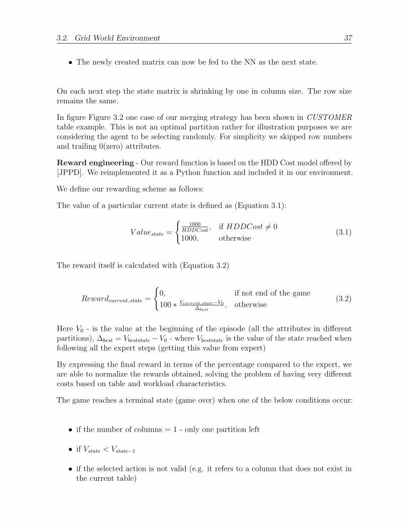
3.2. Grid World Environment 37
• The newly created matrix can now be fed to the NN as the next state.
On each next step the state matrix is shrinking by one in column size. The row sizeremains the same.
In figure Figure 3.2 one case of our merging strategy has been shown in CUSTOMERtable example. This is not an optimal partition rather for illustration purposes we areconsidering the agent to be selecting randomly. For simplicity we skipped row numbersand trailing 0(zero) attributes.
Reward engineering - Our reward function is based on the HDD Cost model offered by[JPPD]. We reimplemented it as a Python function and included it in our environment.
We define our rewarding scheme as follows:
The value of a particular current state is defined as (Equation 3.1):
V aluestate =
{1000
HDDCost, if HDDCost 6= 0
1000, otherwise(3.1)
The reward itself is calculated with (Equation 3.2)
Rewardcurrent state =
{0, if not end of the game
100 ∗ Vcurrent state−V0∆best
, otherwise(3.2)
Here V0 - is the value at the beginning of the episode (all the attributes in differentpartitions), ∆best = Vbeststate− V0 - where Vbeststate is the value of the state reached whenfollowing all the expert steps (getting this value from expert)
By expressing the final reward in terms of the percentage compared to the expert, weare able to normalize the rewards obtained, solving the problem of having very differentcosts based on table and workload characteristics.
The game reaches a terminal state (game over) when one of the below conditions occur:
• if the number of columns = 1 - only one partition left
• if Vstate < Vstate−1
• if the selected action is not valid (e.g. it refers to a column that does not exist inthe current table)
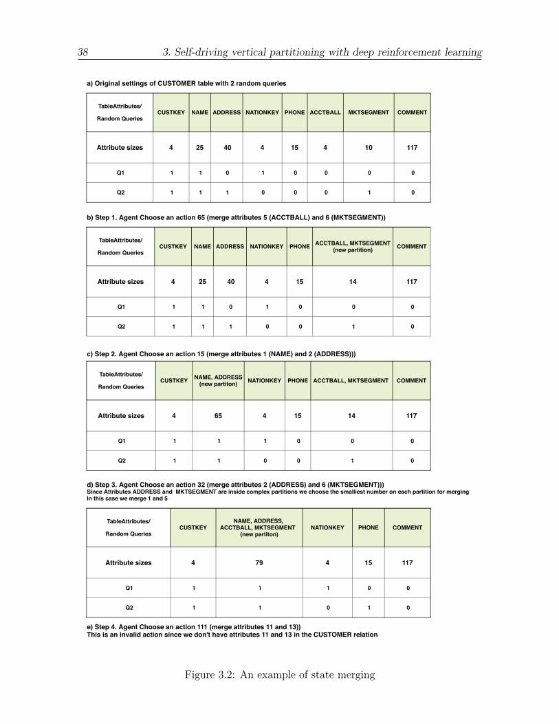
38 3. Self-driving vertical partitioning with deep reinforcement learning
TableAttributes/
Random QueriesCUSTKEY NAME ADDRESS NATIONKEY PHONE ACCTBALL MKTSEGMENT COMMENT
Attribute sizes 4 25 40 4 15 4 10 117
Q1 1 1 0 1 0 0 0 0
Q2 1 1 1 0 0 0 1 0
a) Original settings of CUSTOMER table with 2 random queries
b) Step 1. Agent Choose an action 65 (merge attributes 5 (ACCTBALL) and 6 (MKTSEGMENT))
TableAttributes/
Random QueriesCUSTKEY NAME ADDRESS NATIONKEY PHONE ACCTBALL, MKTSEGMENT
(new partition) COMMENT
Attribute sizes 4 25 40 4 15 14 117
Q1 1 1 0 1 0 0 0
Q2 1 1 1 0 0 1 0
c) Step 2. Agent Choose an action 15 (merge attributes 1 (NAME) and 2 (ADDRESS)))
TableAttributes/
Random QueriesCUSTKEY NAME, ADDRESS
(new partiton) NATIONKEY PHONE ACCTBALL, MKTSEGMENT COMMENT
Attribute sizes 4 65 4 15 14 117
Q1 1 1 1 0 0 0
Q2 1 1 0 0 1 0
e) Step 4. Agent Choose an action 111 (merge attributes 11 and 13))This is an invalid action since we don't have attributes 11 and 13 in the CUSTOMER relation
d) Step 3. Agent Choose an action 32 (merge attributes 2 (ADDRESS) and 6 (MKTSEGMENT))) Since Attributes ADDRESS and MKTSEGMENT are inside complex partitions we choose the smalliest number on each partition for mergingIn this case we merge 1 and 5
TableAttributes/
Random QueriesCUSTKEY
NAME, ADDRESS, ACCTBALL, MKTSEGMENT
(new partiton)NATIONKEY PHONE COMMENT
Attribute sizes 4 79 4 15 117
Q1 1 1 1 0 0
Q2 1 1 0 1 0
Figure 3.2: An example of state merging
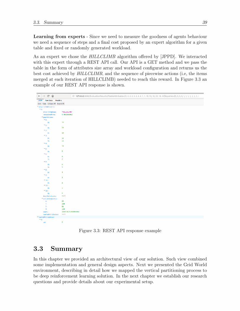
3.3. Summary 39
Learning from experts - Since we need to measure the goodness of agents behaviourwe need a sequence of steps and a final cost proposed by an expert algorithm for a giventable and fixed or randomly generated workload.
As an expert we chose the HILLCLIMB algorithm offered by [JPPD]. We interactedwith this expert through a REST API call. Our API is a GET method and we pass thetable in the form of attributes size array and workload configuration and returns us thebest cost achieved by HILLCLIMB, and the sequence of piecewise actions (i.e, the itemsmerged at each iteration of HILLCLIMB) needed to reach this reward. In Figure 3.3 anexample of our REST API response is shown.
Figure 3.3: REST API response example
3.3 Summary
In this chapter we provided an architectural view of our solution. Such view combinedsome implementation and general design aspects. Next we presented the Grid Worldenvironment, describing in detail how we mapped the vertical partitioning process tobe deep reinforcement learning solution. In the next chapter we establish our researchquestions and provide details about our experimental setup.

40 3. Self-driving vertical partitioning with deep reinforcement learning
4. Experimental setup
In this chapter we establish our research questions and overview the experimental setupwe used for evaluation.
The chapter is organized as follows:
• Research Questions:First we provide several research questions that we aim to address in our work(Section 4.1).
• Hyper-parameters for DQN agents:We define how the DQN agents are configured in our experiments (Section 4.2).
• Unified settings for proposed algorithms:We discuss adapted and unified versions of vertical partitioning algorithms discussedin (Section 2.2), which were required for our evaluation ().
• Measurement Process:We introduce our basic measurement methodology (Section 4.4).
• Evaluation Environment:We list relevant characteristics from the execution environment of our tests (Sec-tion 4.5).
• Benchmarks:We describe the TPC-H benchmark which has been used for our evaluations(Section 4.6).
• Summary:We conclude the whole chapter in (Section 4.7).
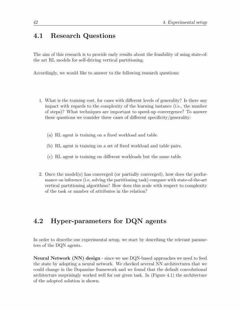
42 4. Experimental setup
4.1 Research Questions
The aim of this research is to provide early results about the feasibility of using state-of-the art RL models for self-driving vertical partitioning.
Accordingly, we would like to answer to the following research questions:
1. What is the training cost, for cases with different levels of generality? Is there anyimpact with regards to the complexity of the learning instance (i.e., the numberof steps)? What techniques are important to speed-up convergence? To answerthese questions we consider three cases of different specificity/generality:
(a) RL agent is training on a fixed workload and table.
(b) RL agent is training on a set of fixed workload and table pairs.
(c) RL agent is training on different workloads but the same table.
2. Once the model(s) has converged (or partially converged), how does the perfor-mance on inference (i.e, solving the partitioning task) compare with state-of-the-artvertical partitioning algorithms? How does this scale with respect to complexityof the task or number of attributes in the relation?
4.2 Hyper-parameters for DQN agents
In order to describe our experimental setup, we start by describing the relevant parame-ters of the DQN agents.
Neural Network (NN) design - since we use DQN-based approaches we need to feedthe state by adopting a neural network. We checked several NN architectures that wecould change in the Dopamine framework and we found that the default convolutionalarchitecture surprisingly worked well for our given task. In (Figure 4.1) the architectureof the adopted solution is shown.
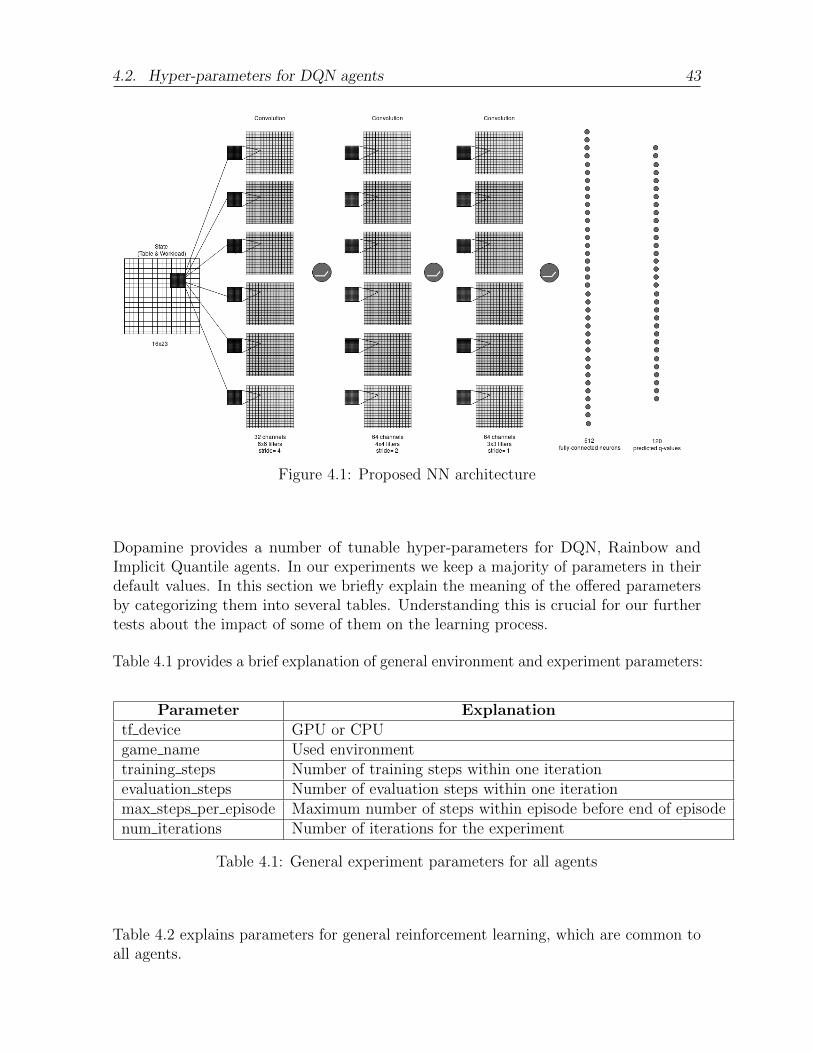
4.2. Hyper-parameters for DQN agents 43
Figure 4.1: Proposed NN architecture
Dopamine provides a number of tunable hyper-parameters for DQN, Rainbow andImplicit Quantile agents. In our experiments we keep a majority of parameters in theirdefault values. In this section we briefly explain the meaning of the offered parametersby categorizing them into several tables. Understanding this is crucial for our furthertests about the impact of some of them on the learning process.
Table 4.1 provides a brief explanation of general environment and experiment parameters:
Parameter Explanationtf device GPU or CPUgame name Used environmenttraining steps Number of training steps within one iterationevaluation steps Number of evaluation steps within one iterationmax steps per episode Maximum number of steps within episode before end of episodenum iterations Number of iterations for the experiment
Table 4.1: General experiment parameters for all agents
Table 4.2 explains parameters for general reinforcement learning, which are common toall agents.
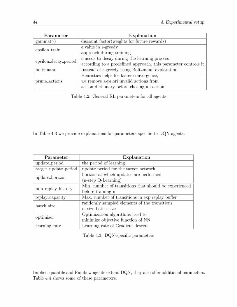
44 4. Experimental setup
Parameter Explanationgamma(γ) discount factor(weights for future rewards)
epsilon trainε value in ε-greedyapproach during training
epsilon decay periodε needs to decay during the learning processaccording to a predefined approach, this parameter controls it
boltzmann Instead of ε-greedy using Boltzmann exploration
prune actionsHeuristics helps for faster convergence,we remove a-priori invalid actions fromaction dictionary before chosing an action
Table 4.2: General RL parameters for all agents
In Table 4.3 we provide explanations for parameters specific to DQN agents.
Parameter Explanationupdate period the period of learningtarget update period update period for the target network
update horizonhorizon at which updates are performed(n-step Q-Learning)
min replay historyMin. number of transitions that should be experiencedbefore training n
replay capacity Max. number of transitions in exp.replay buffer
batch sizerandomly sampled elements of the transitionsof size batch size
optimizerOptimization algorithms used tominimize objective function of NN
learning rate Learning rate of Gradient descent
Table 4.3: DQN-specific parameters
Implicit quantile and Rainbow agents extend DQN, they also offer additional parameters.Table 4.4 shows some of these parameters.
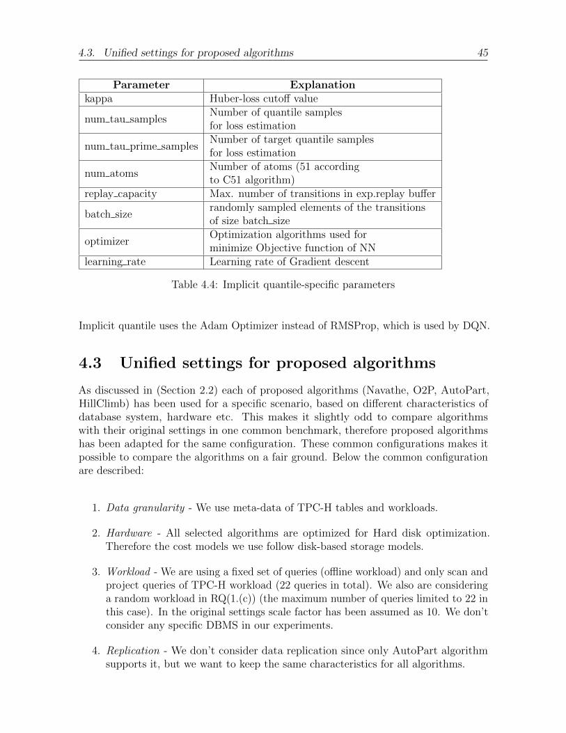
4.3. Unified settings for proposed algorithms 45
Parameter Explanationkappa Huber-loss cutoff value
num tau samplesNumber of quantile samplesfor loss estimation
num tau prime samplesNumber of target quantile samplesfor loss estimation
num atomsNumber of atoms (51 accordingto C51 algorithm)
replay capacity Max. number of transitions in exp.replay buffer
batch sizerandomly sampled elements of the transitionsof size batch size
optimizerOptimization algorithms used forminimize Objective function of NN
learning rate Learning rate of Gradient descent
Table 4.4: Implicit quantile-specific parameters
Implicit quantile uses the Adam Optimizer instead of RMSProp, which is used by DQN.
4.3 Unified settings for proposed algorithms
As discussed in (Section 2.2) each of proposed algorithms (Navathe, O2P, AutoPart,HillClimb) has been used for a specific scenario, based on different characteristics ofdatabase system, hardware etc. This makes it slightly odd to compare algorithmswith their original settings in one common benchmark, therefore proposed algorithmshas been adapted for the same configuration. These common configurations makes itpossible to compare the algorithms on a fair ground. Below the common configurationare described:
1. Data granularity - We use meta-data of TPC-H tables and workloads.
2. Hardware - All selected algorithms are optimized for Hard disk optimization.Therefore the cost models we use follow disk-based storage models.
3. Workload - We are using a fixed set of queries (offline workload) and only scan andproject queries of TPC-H workload (22 queries in total). We also are consideringa random workload in RQ(1.(c)) (the maximum number of queries limited to 22 inthis case). In the original settings scale factor has been assumed as 10. We don’tconsider any specific DBMS in our experiments.
4. Replication - We don’t consider data replication since only AutoPart algorithmsupports it, but we want to keep the same characteristics for all algorithms.
46 4. Experimental setup
4.4 Measurement Process
In our evaluation we focus on convergence time and inference time of our agents aswell as time need to be able (for the traditional algorithms) to formulate the partitions.Since our implementation contains both Java and Python parts we use:
• System.nanoTime() - Java system timer provide sufficient precision.
• from timeit import default timer as timer - measure execution time for Python
To guarantee more reliable results we replay each experiments several times, and disclosethe number of repetitions in each case.
4.5 Experiment Environment
Our experiments were executed on a multi-core machine running on Ubuntu 16.04system. Detailed parameters of the system as well as used software versions are givenbelow:
• Intel R© CoreTM i7-6700HQ CPU @ 2.60GHz 8 (8 cores in total
• RAM - 15.5 GiB of memory
• GPU - GeForce GTX 960M/PCIe/SSE2
• Java version: Java SDK 8u111-linux-x64
• Python version:Python3.5
• Dopamine framework: Dopamine 1.0.5
• Tensorflow: Tensorflow-GPU 1.12.0
• Numpy 1.15.4
• Gym 0.10.9
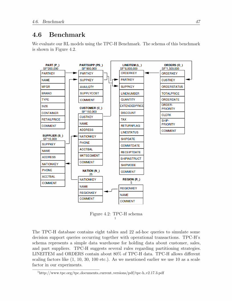
4.6. Benchmark 47
4.6 Benchmark
We evaluate our RL models using the TPC-H Benchmark. The schema of this benchmarkis shown in Figure 4.2.
Figure 4.2: TPC-H schema1
The TPC-H database contains eight tables and 22 ad-hoc queries to simulate somedecision support queries occurring together with operational transactions. TPC-H’sschema represents a simple data warehouse for holding data about customer, sales,and part suppliers. TPC-H suggests several rules regarding partitioning strategies.LINEITEM and ORDERS contain about 80% of TPC-H data. TPC-H allows differentscaling factors like (1, 10, 30, 100 etc.). As we mentioned earlier we use 10 as a scalefactor in our experiments.
1http://www.tpc.org/tpc documents current versions/pdf/tpc-h v2.17.3.pdf

48 4. Experimental setup
4.7 Summary
In this chapter we introduce our research questions. Next we describe parameters, unifiedsettings for vertical partititioning algorithms, the measurement process, benchmarks weused and finally parameters of the hardware that we use for our evaluations.
5. Evaluation and Results
In this chapter we discuss the evaluation and results of our experiments. This chaptercontains two parts:
• In (Section 5.1) we discuss problems related to training costs, convergence resultsand the impact of task complexity for the three cases of generality discussed inRQ 1.
• In (Section 5.2) we compare the performance of our learning models in terms ofsolving partitioning tasks with state-of-the-art vertical partition algorithms.
5.1 Training of models
In this evaluation section we focus on our first research question. We test different factorswhich might have potential influence for our models convergence and performance. Asdiscussed in Chapter 4 we use the Dopamine framework and use models offered byDopamine.In our evaluations we used three DRL agents:
• Deep Q-Network (DQN)
• Rainbow
• Implicit Quantile
Rainbow and Implicit Quantile agents extend the DQN agent but also add additionalhyper-parameters for tuning. Since, the network architecture used inside these modelsaremainly based on convolutional architecture offered by Dopamine therefore we keep allparameters of network as it is.
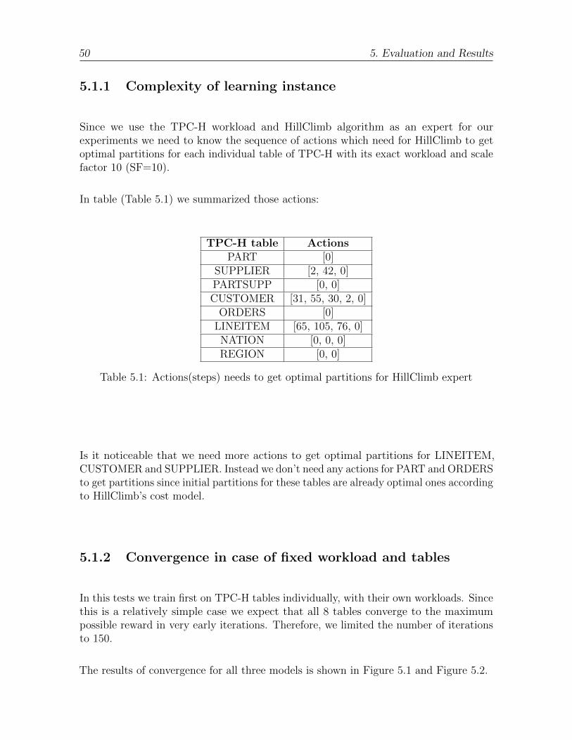
50 5. Evaluation and Results
5.1.1 Complexity of learning instance
Since we use the TPC-H workload and HillClimb algorithm as an expert for ourexperiments we need to know the sequence of actions which need for HillClimb to getoptimal partitions for each individual table of TPC-H with its exact workload and scalefactor 10 (SF=10).
In table (Table 5.1) we summarized those actions:
TPC-H table ActionsPART [0]
SUPPLIER [2, 42, 0]PARTSUPP [0, 0]CUSTOMER [31, 55, 30, 2, 0]
ORDERS [0]LINEITEM [65, 105, 76, 0]NATION [0, 0, 0]REGION [0, 0]
Table 5.1: Actions(steps) needs to get optimal partitions for HillClimb expert
Is it noticeable that we need more actions to get optimal partitions for LINEITEM,CUSTOMER and SUPPLIER. Instead we don’t need any actions for PART and ORDERSto get partitions since initial partitions for these tables are already optimal ones accordingto HillClimb’s cost model.
5.1.2 Convergence in case of fixed workload and tables
In this tests we train first on TPC-H tables individually, with their own workloads. Sincethis is a relatively simple case we expect that all 8 tables converge to the maximumpossible reward in very early iterations. Therefore, we limited the number of iterationsto 150.
The results of convergence for all three models is shown in Figure 5.1 and Figure 5.2.
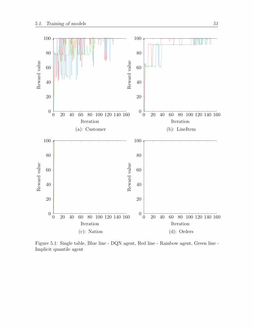
5.1. Training of models 51
0 20 40 60 80 100 120 140 1600
20
40
60
80
100
Iteration
Rew
ard
valu
e
0 20 40 60 80 100 120 140 1600
20
40
60
80
100
Iteration
Rew
ard
valu
e
0 20 40 60 80 100 120 140 1600
20
40
60
80
100
Iteration
Rew
ard
valu
e
0 20 40 60 80 100 120 140 1600
20
40
60
80
100
Iteration
Rew
ard
valu
e(a): Customer (b): LineItem
(c): Nation (d): Orders
Figure 5.1: Single table, Blue line - DQN agent, Red line - Rainbow agent, Green line -Implicit quantile agent
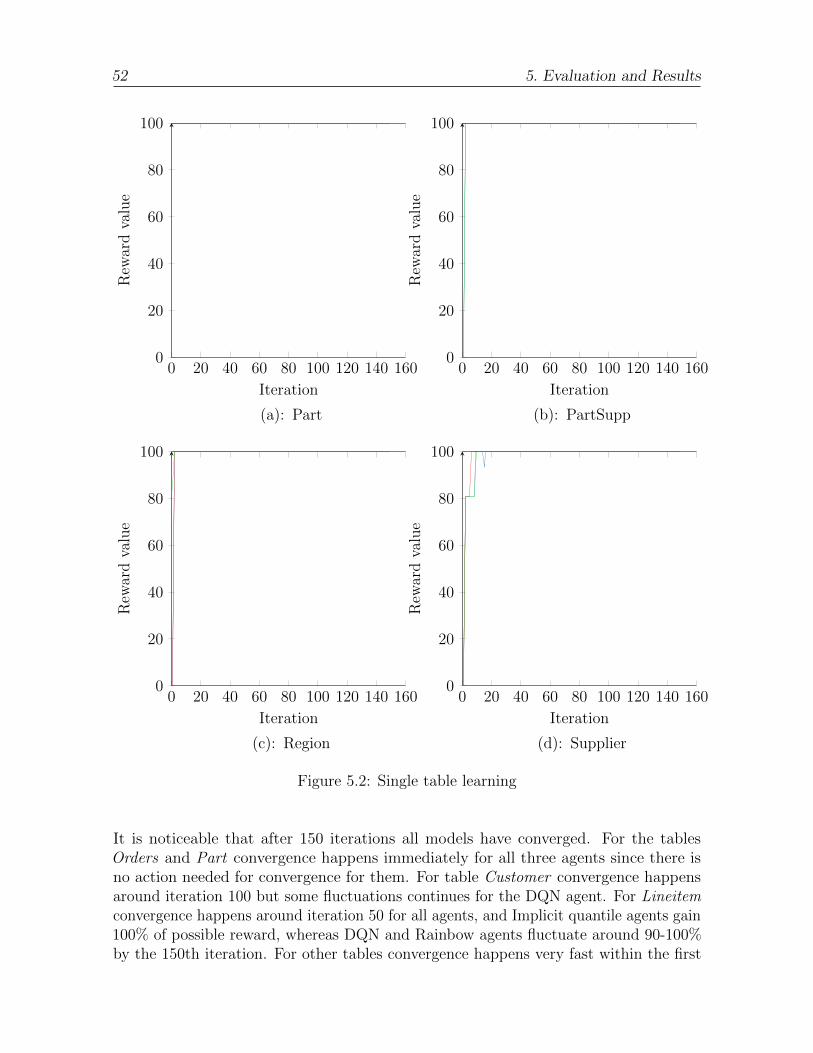
52 5. Evaluation and Results
0 20 40 60 80 100 120 140 1600
20
40
60
80
100
Iteration
Rew
ard
valu
e
0 20 40 60 80 100 120 140 1600
20
40
60
80
100
Iteration
Rew
ard
valu
e
0 20 40 60 80 100 120 140 1600
20
40
60
80
100
Iteration
Rew
ard
valu
e
0 20 40 60 80 100 120 140 1600
20
40
60
80
100
Iteration
Rew
ard
valu
e(a): Part (b): PartSupp
(c): Region (d): Supplier
Figure 5.2: Single table learning
It is noticeable that after 150 iterations all models have converged. For the tablesOrders and Part convergence happens immediately for all three agents since there isno action needed for convergence for them. For table Customer convergence happensaround iteration 100 but some fluctuations continues for the DQN agent. For Lineitemconvergence happens around iteration 50 for all agents, and Implicit quantile agents gain100% of possible reward, whereas DQN and Rainbow agents fluctuate around 90-100%by the 150th iteration. For other tables convergence happens very fast within the first
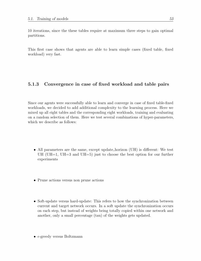
5.1. Training of models 53
10 iterations, since the these tables require at maximum three steps to gain optimalpartitions.
This first case shows that agents are able to learn simple cases (fixed table, fixedworkload) very fast.
5.1.3 Convergence in case of fixed workload and table pairs
Since our agents were successfully able to learn and converge in case of fixed table-fixedworkloads, we decided to add additional complexity to the learning process. Here wemixed up all eight tables and the corresponding eight workloads, training and evaluatingon a random selection of them. Here we test several combinations of hyper-parameters,which we describe as follows:
• All parameters are the same, except update horizon (UH) is different: We testUH (UH=1, UH=3 and UH=5) just to choose the best option for our furtherexperiments
• Prune actions versus non prune actions
• Soft-update versus hard-update: This refers to how the synchronization betweencurrent and target network occurs. In a soft update the synchronization occurson each step, but instead of weights being totally copied within one network andanother, only a small percentage (tau) of the weights gets updated.
• ε-greedy versus Boltzmann
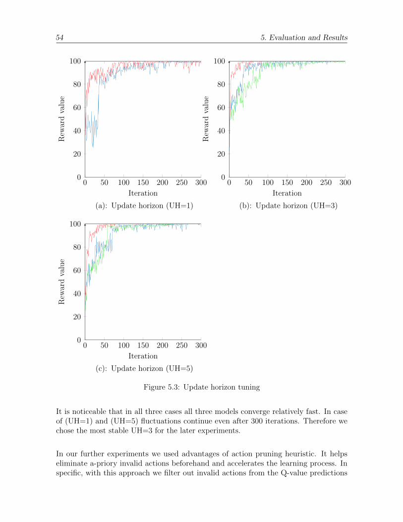
54 5. Evaluation and Results
0 50 100 150 200 250 3000
20
40
60
80
100
Iteration
Rew
ard
valu
e
0 50 100 150 200 250 3000
20
40
60
80
100
Iteration
Rew
ard
valu
e
0 50 100 150 200 250 3000
20
40
60
80
100
Iteration
Rew
ard
valu
e
(a): Update horizon (UH=1) (b): Update horizon (UH=3)
(c): Update horizon (UH=5)
Figure 5.3: Update horizon tuning
It is noticeable that in all three cases all three models converge relatively fast. In caseof (UH=1) and (UH=5) fluctuations continue even after 300 iterations. Therefore wechose the most stable UH=3 for the later experiments.
In our further experiments we used advantages of action pruning heuristic. It helpseliminate a-priory invalid actions beforehand and accelerates the learning process. Inspecific, with this approach we filter out invalid actions from the Q-value predictions
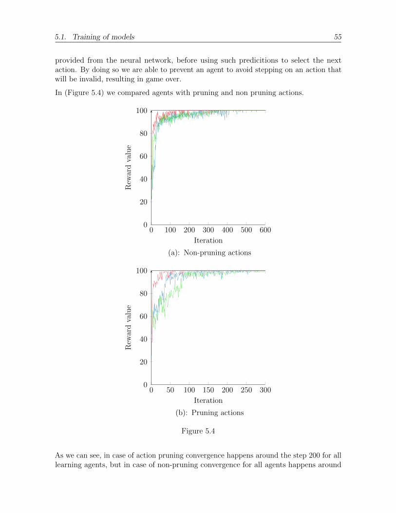
5.1. Training of models 55
provided from the neural network, before using such predicitions to select the nextaction. By doing so we are able to prevent an agent to avoid stepping on an action thatwill be invalid, resulting in game over.
In (Figure 5.4) we compared agents with pruning and non pruning actions.
0 100 200 300 400 500 6000
20
40
60
80
100
Iteration
Rew
ard
valu
e
0 50 100 150 200 250 3000
20
40
60
80
100
Iteration
Rew
ard
valu
e
(a): Non-pruning actions
(b): Pruning actions
Figure 5.4
As we can see, in case of action pruning convergence happens around the step 200 for alllearning agents, but in case of non-pruning convergence for all agents happens around
56 5. Evaluation and Results
400. Therefore, for the next experiments we keep the action pruning heuristic for fasterlearning.
The next set of experiments were dedicated to comparing hard versus soft update ofweights from the NN. In the case of hard-updates we follow the fixed-Q-target strategywhere we move weights of learning value network to target value network after certainamount of time described via the hyper parameter target update period.
In case of soft-update we follow the same strategy but also change targets weight veryslightly gradually on every step.
In Figure 5.5 we compared agents with hard and soft updates.
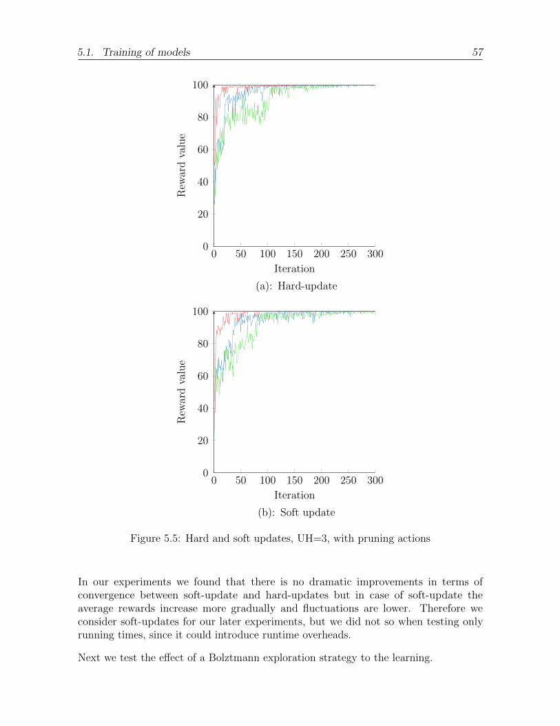
5.1. Training of models 57
0 50 100 150 200 250 3000
20
40
60
80
100
Iteration
Rew
ard
valu
e
0 50 100 150 200 250 3000
20
40
60
80
100
Iteration
Rew
ard
valu
e
(a): Hard-update
(b): Soft update
Figure 5.5: Hard and soft updates, UH=3, with pruning actions
In our experiments we found that there is no dramatic improvements in terms ofconvergence between soft-update and hard-updates but in case of soft-update theaverage rewards increase more gradually and fluctuations are lower. Therefore weconsider soft-updates for our later experiments, but we did not so when testing onlyrunning times, since it could introduce runtime overheads.
Next we test the effect of a Bolztmann exploration strategy to the learning.
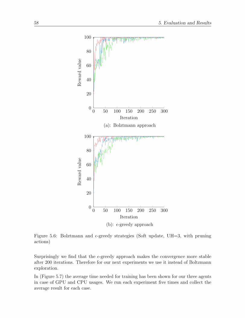
58 5. Evaluation and Results
0 50 100 150 200 250 3000
20
40
60
80
100
Iteration
Rew
ard
valu
e
0 50 100 150 200 250 3000
20
40
60
80
100
Iteration
Rew
ard
valu
e
(a): Bolztmann approach
(b): ε-greedy approach
Figure 5.6: Bolztmann and ε-greedy strategies (Soft update, UH=3, with pruningactions)
Surprisingly we find that the ε-greedy approach makes the convergence more stableafter 200 iterations. Therefore for our next experiments we use it instead of Boltzmannexploration.
In (Figure 5.7) the average time needed for training has been shown for our three agentsin case of GPU and CPU usages. We run each experiment five times and collect theaverage result for each case.
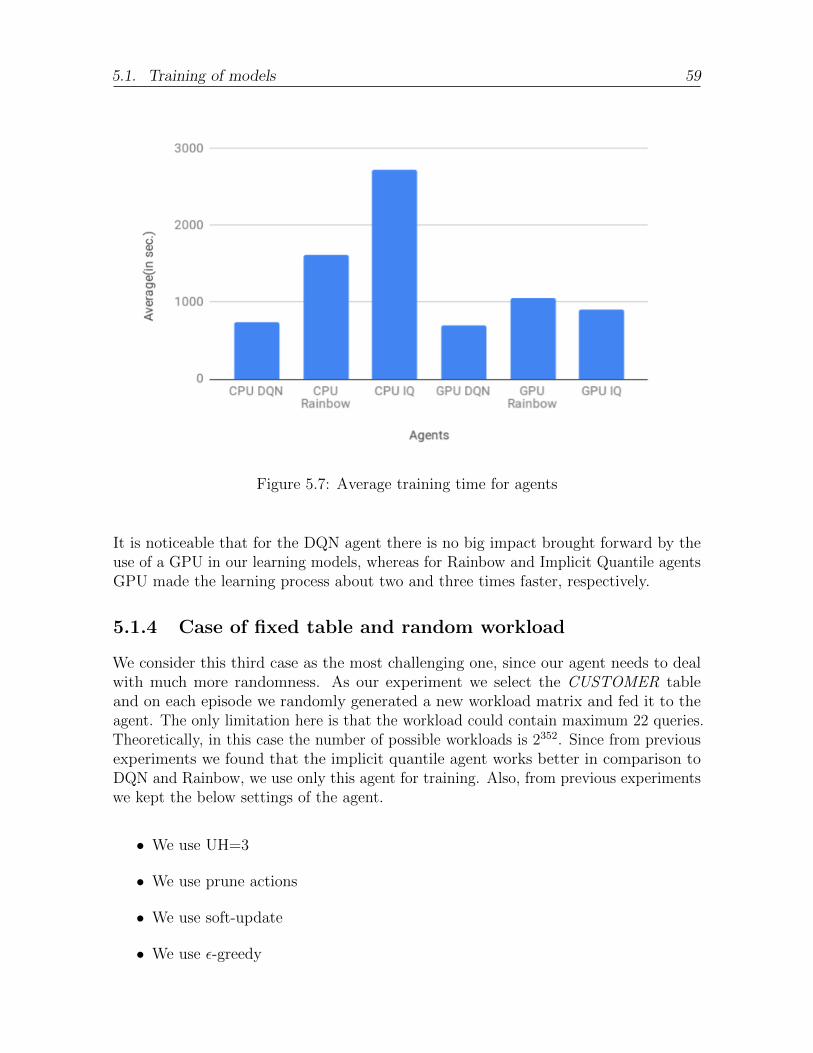
5.1. Training of models 59
Figure 5.7: Average training time for agents
It is noticeable that for the DQN agent there is no big impact brought forward by theuse of a GPU in our learning models, whereas for Rainbow and Implicit Quantile agentsGPU made the learning process about two and three times faster, respectively.
5.1.4 Case of fixed table and random workload
We consider this third case as the most challenging one, since our agent needs to dealwith much more randomness. As our experiment we select the CUSTOMER tableand on each episode we randomly generated a new workload matrix and fed it to theagent. The only limitation here is that the workload could contain maximum 22 queries.Theoretically, in this case the number of possible workloads is 2352. Since from previousexperiments we found that the implicit quantile agent works better in comparison toDQN and Rainbow, we use only this agent for training. Also, from previous experimentswe kept the below settings of the agent.
• We use UH=3
• We use prune actions
• We use soft-update
• We use ε-greedy
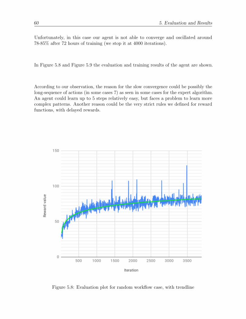
60 5. Evaluation and Results
Unfortunately, in this case our agent is not able to converge and oscillated around78-85% after 72 hours of training (we stop it at 4000 iterations).
In Figure 5.8 and Figure 5.9 the evaluation and training results of the agent are shown.
According to our observation, the reason for the slow convergence could be possibly thelong-sequence of actions (in some cases 7) as seen in some cases for the expert algorithm.An agent could learn up to 5 steps relatively easy, but faces a problem to learn morecomplex patterns. Another reason could be the very strict rules we defined for rewardfunctions, with delayed rewards.
Figure 5.8: Evaluation plot for random workflow case, with trendline
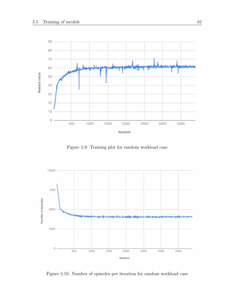
5.1. Training of models 61
Figure 5.9: Training plot for random workload case
Figure 5.10: Number of episodes per iteration for random workload case
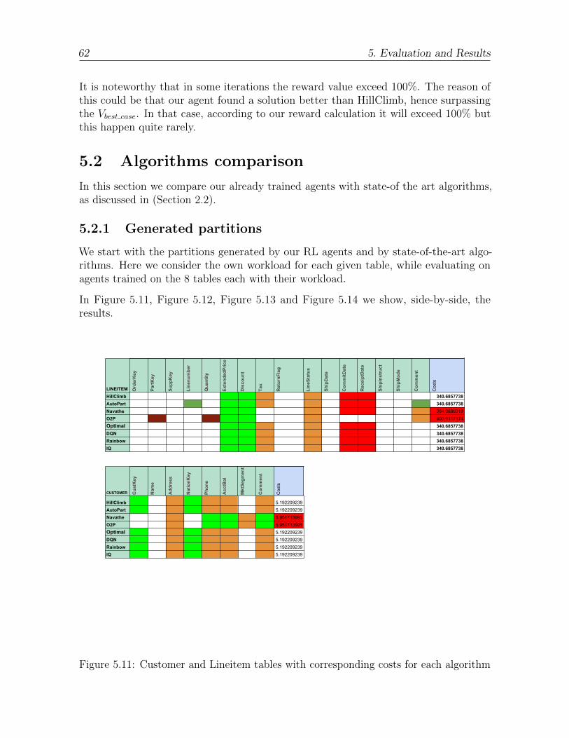
62 5. Evaluation and Results
It is noteworthy that in some iterations the reward value exceed 100%. The reason ofthis could be that our agent found a solution better than HillClimb, hence surpassingthe Vbest case. In that case, according to our reward calculation it will exceed 100% butthis happen quite rarely.
5.2 Algorithms comparison
In this section we compare our already trained agents with state-of the art algorithms,as discussed in (Section 2.2).
5.2.1 Generated partitions
We start with the partitions generated by our RL agents and by state-of-the-art algo-rithms. Here we consider the own workload for each given table, while evaluating onagents trained on the 8 tables each with their workload.
In Figure 5.11, Figure 5.12, Figure 5.13 and Figure 5.14 we show, side-by-side, theresults.
LINEITEM OrderKey
PartKey
Supp
Key
Linenu
mber
Quantity
Extend
edPrice
Discoun
t
Tax
ReturnF
lag
LineStatus
ShipDate
Com
mitD
ate
ReceiptDate
ShipInstruct
ShipMod
e
Com
ment
Costs
HillClimb 340.6857738AutoPart 340.6857738Navathe 384.9696318O2P 400.6117174Optimal 340.6857738DQN 340.6857738Rainbow 340.6857738IQ 340.6857738
CUSTOMER CustKey
Nam
e
Add
ress
NationK
ey
Phon
e
AcctBal
MktSe
gment
Com
ment
Costs
HillClimb 5.192209239AutoPart 5.192209239Navathe 5.951713995O2P 5.951713995Optimal 5.192209239DQN 5.192209239Rainbow 5.192209239IQ 5.192209239
Figure 5.11: Customer and Lineitem tables with corresponding costs for each algorithm
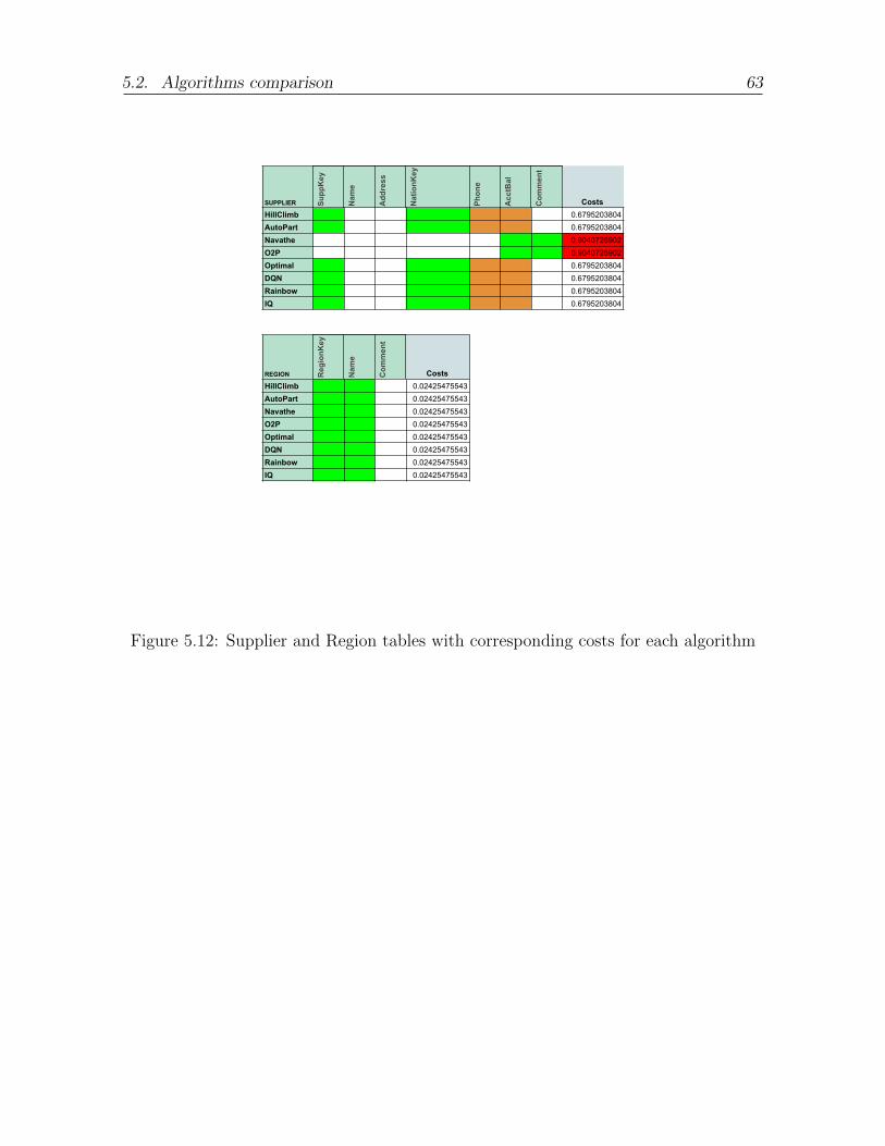
5.2. Algorithms comparison 63
SUPPLIER Supp
Key
Nam
e
Add
ress
NationK
ey
Phon
e
AcctBal
Com
ment
CostsHillClimb 0.6795203804AutoPart 0.6795203804Navathe 0.9040726902O2P 0.9040726902Optimal 0.6795203804DQN 0.6795203804Rainbow 0.6795203804IQ 0.6795203804
REGION RegionK
ey
Nam
e
Com
ment
CostsHillClimb 0.02425475543AutoPart 0.02425475543Navathe 0.02425475543O2P 0.02425475543Optimal 0.02425475543DQN 0.02425475543Rainbow 0.02425475543IQ 0.02425475543
Figure 5.12: Supplier and Region tables with corresponding costs for each algorithm
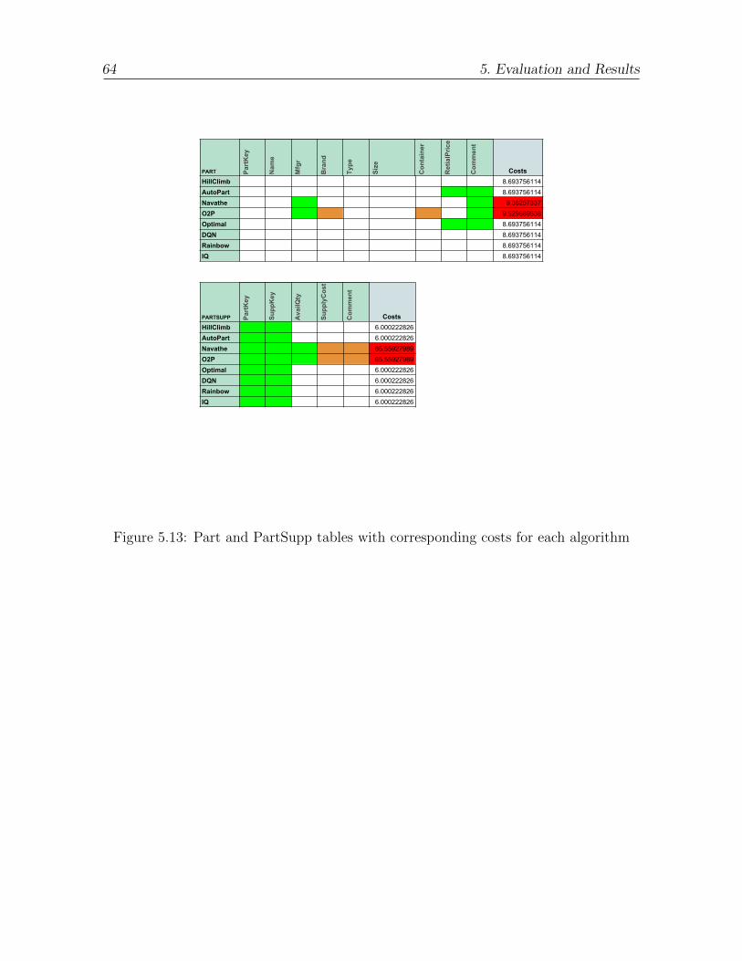
64 5. Evaluation and Results
PART PartKey
Nam
e
Mfgr
Brand
Type
Size
Con
tainer
RetialPric
e
Com
ment
CostsHillClimb 8.693756114AutoPart 8.693756114Navathe 9.36257337O2P 9.529689538Optimal 8.693756114DQN 8.693756114Rainbow 8.693756114IQ 8.693756114
PARTSUPP PartKey
Supp
Key
AvailQ
ty
Supp
lyCost
Com
ment
CostsHillClimb 6.000222826AutoPart 6.000222826Navathe 65.55927989O2P 65.55927989Optimal 6.000222826DQN 6.000222826Rainbow 6.000222826IQ 6.000222826
Figure 5.13: Part and PartSupp tables with corresponding costs for each algorithm
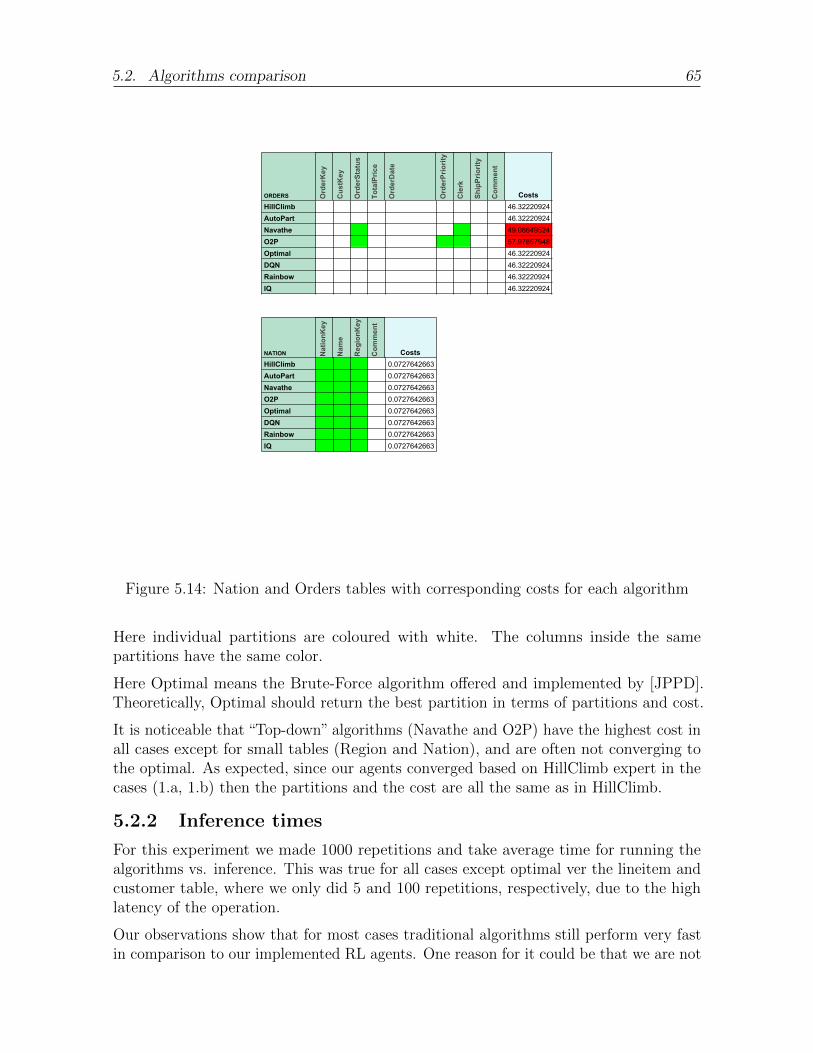
5.2. Algorithms comparison 65
ORDERS OrderKey
CustKey
OrderStatus
TotalPric
e
OrderDate
OrderPriority
Clerk
ShipPriority
Com
ment
CostsHillClimb 46.32220924AutoPart 46.32220924Navathe 49.08649524O2P 57.97857948Optimal 46.32220924DQN 46.32220924Rainbow 46.32220924IQ 46.32220924
NATION NationK
ey
Nam
e
RegionK
ey
Com
ment
CostsHillClimb 0.0727642663AutoPart 0.0727642663Navathe 0.0727642663O2P 0.0727642663Optimal 0.0727642663DQN 0.0727642663Rainbow 0.0727642663IQ 0.0727642663
Figure 5.14: Nation and Orders tables with corresponding costs for each algorithm
Here individual partitions are coloured with white. The columns inside the samepartitions have the same color.
Here Optimal means the Brute-Force algorithm offered and implemented by [JPPD].Theoretically, Optimal should return the best partition in terms of partitions and cost.
It is noticeable that “Top-down” algorithms (Navathe and O2P) have the highest cost inall cases except for small tables (Region and Nation), and are often not converging tothe optimal. As expected, since our agents converged based on HillClimb expert in thecases (1.a, 1.b) then the partitions and the cost are all the same as in HillClimb.
5.2.2 Inference times
For this experiment we made 1000 repetitions and take average time for running thealgorithms vs. inference. This was true for all cases except optimal ver the lineitem andcustomer table, where we only did 5 and 100 repetitions, respectively, due to the highlatency of the operation.
Our observations show that for most cases traditional algorithms still perform very fastin comparison to our implemented RL agents. One reason for it could be that we are not
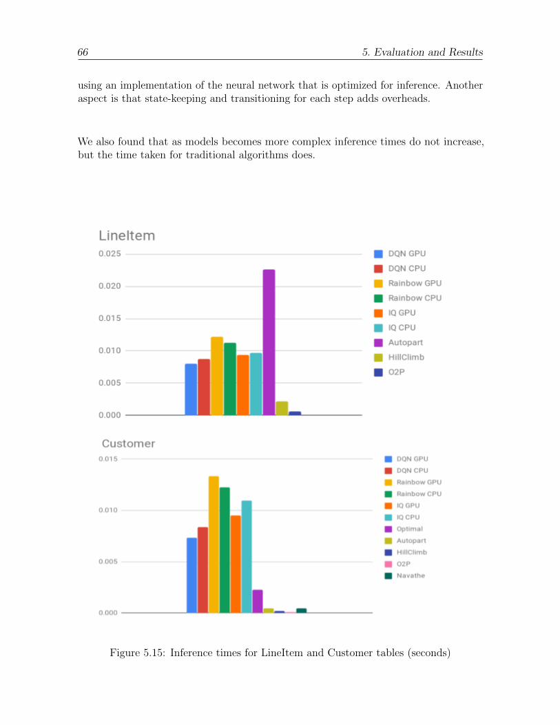
66 5. Evaluation and Results
using an implementation of the neural network that is optimized for inference. Anotheraspect is that state-keeping and transitioning for each step adds overheads.
We also found that as models becomes more complex inference times do not increase,but the time taken for traditional algorithms does.
Figure 5.15: Inference times for LineItem and Customer tables (seconds)
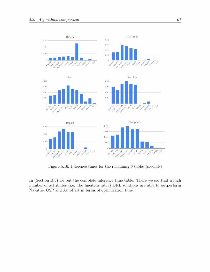
5.2. Algorithms comparison 67
Figure 5.16: Inference times for the remaining 6 tables (seconds)
In (Section B.3) we put the complete inference time table. There we see that a highnumber of attributes (i.e. the lineitem table) DRL solutions are able to outperformNavathe, O2P and AutoPart in terms of optimization time.
68 5. Evaluation and Results
5.3 Summary
In this chapter we discuss the evaluation and results of our experiments. First we checkedthe possibility of our agents to learn in three cases with different hyper-parameters. Weobserve that in the first two cases agents are able to converge relatively easy. But in themost complex case we evaluated, we did not find a 100% convergence. In spite of thisresult we are able to find some cases where our solution outperforms, during training,HillClimb.
In the second part of chapter we compared partitions and the cost need to achieve thesepartitions. We found that our “top-down” algorithms result in less efficient solutionsin comparison to “bottom-up” ones, in most cases. We also observe that partitionsgenerated by our learning agents are exactly the same as for the expert HillClimbalgorithm, matching the optima. This proves that our agents correctly converge and atsimple cases are able to mimic the behavior of an expert.
We tested inference times for each table and its default workload. Results show thatimprovements in the implementation of the inference procedure will be required (includingimprovements for state-transitions) to make DRL-based solutions also competitive interms of inference time.
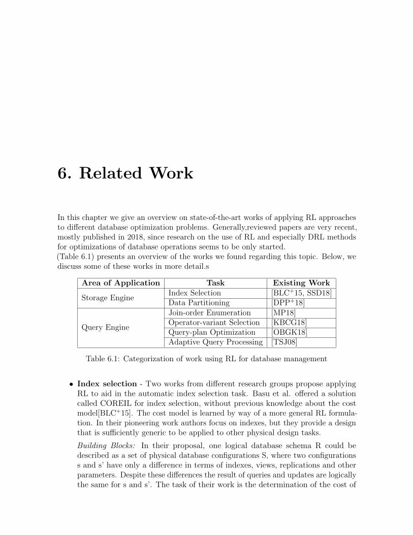
6. Related Work
In this chapter we give an overview on state-of-the-art works of applying RL approachesto different database optimization problems. Generally,reviewed papers are very recent,mostly published in 2018, since research on the use of RL and especially DRL methodsfor optimizations of database operations seems to be only started.(Table 6.1) presents an overview of the works we found regarding this topic. Below, wediscuss some of these works in more detail.s
Area of Application Task Existing Work
Storage EngineIndex Selection [BLC+15, SSD18]Data Partitioning [DPP+18]
Query Engine
Join-order Enumeration [MP18]Operator-variant Selection [KBCG18]Query-plan Optimization [OBGK18]Adaptive Query Processing [TSJ08]
Table 6.1: Categorization of work using RL for database management
• Index selection - Two works from different research groups propose applyingRL to aid in the automatic index selection task. Basu et al. offered a solutioncalled COREIL for index selection, without previous knowledge about the costmodel[BLC+15]. The cost model is learned by way of a more general RL formula-tion. In their pioneering work authors focus on indexes, but they provide a designthat is sufficiently generic to be applied to other physical design tasks.
Building Blocks: In their proposal, one logical database schema R could bedescribed as a set of physical database configurations S, where two configurationss and s’ have only a difference in terms of indexes, views, replications and otherparameters. Despite these differences the result of queries and updates are logicallythe same for s and s’. The task of their work is the determination of the cost of
70 6. Related Work
changing from one physical configuration to another, alongside the benefits of theaction. As a workload set Q they considered a stack of queries and updates. Thecost of execution of query q on the configuration s is denoted as cost(s,q). Theymodeled query q as a random variable which only becomes observable at the timet. The environment for training the model is initialized with a randomly choseninitial configuration, s0 . Authors describe the transition process as a four stepalgorithm: Transitions from one state to another are deterministic. Penalties andrewards, however, are considered stochastic and uncertain.
Based on the formulation described above, the RL problem is framed as that offinding the sequence of configurations that minimizes the sum of per-stage costs.To find an optimal policy, authors adopted a policy iteration approach.
Evaluation: Authors implemented a prototype and compare the results withthe WFIT algorithm, which they identify as state-of-the-art for automatic indexselection. As a dataset they used the TPC-C specification with scale factor 2,with transactions consisting of 5 queries (mixing updates and queries) from anOLTP-bench generated workload. Authors evaluate the process from 0 to 3000transactions. As database authors used IBM DB2.
Results shows that despite COREIL converges slower than WFIT, it can achieveless processing time after convergence (at around 2000 transactions) with onlya small amount of peaks (i.e. cases where it does not achieve better runtimeper transaction than WFIT). After convergence COREIL does not induce highercosts (to create indexes) than does WFIT. However the runtime for making aninference exceeds WFIT by at least an order of magnitude. However, COREIL ismore effective than WFIT because it creates shorter-compound-attribute indexes.Authors conclude that despite COREIL uses a non existent cost-model beforehand,learning it iteratively, its performance is comparable with WFIT. Finally, it shouldalso be noted that the slow convergence of COREIL is feasibly improvable bystarting with cost approximations that are close to the real case.
More recently, Sharma et al. offered the concept of NoDBA [SSD18] which alsoseeks to automate physical design for indexing, based on Deep Reinforcementlearning approaches.
Building Blocks: They assume a database schema S which contains n columns,and the maximum number of indexes is k (k<n). The workload has almost thesame meaning as proposed in Basu et al., except for taking more queries intoconsideration (i.e., a set of n queries, each described by the usage of certain columns,and the selectivity of their predicates on those columns). As input parametersof Neural networks they proposed the workload and the current configurationof indexes separately: Iworkload and Iindexes accordingly. Iworkload is a matrixof n*m where n is the number of queries, and m is number of columns in thedatabase schema. As an element of the matrix they propose the selectivity functionSel(Qi;Cj), whose arguments are: the i-th query and the j-th column. Selectivitiesare computed for every query once per input. Iindexes is a bitlist of size m and
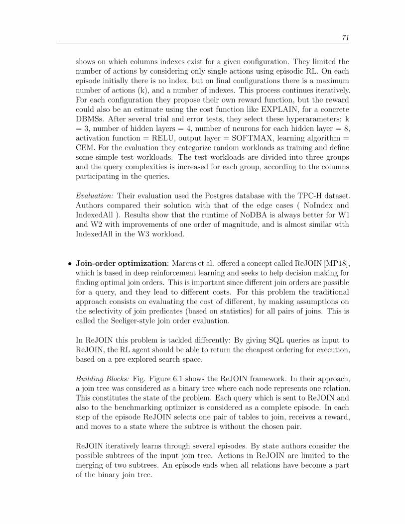
71
shows on which columns indexes exist for a given configuration. They limited thenumber of actions by considering only single actions using episodic RL. On eachepisode initially there is no index, but on final configurations there is a maximumnumber of actions (k), and a number of indexes. This process continues iteratively.For each configuration they propose their own reward function, but the rewardcould also be an estimate using the cost function like EXPLAIN, for a concreteDBMSs. After several trial and error tests, they select these hyperarameters: k= 3, number of hidden layers = 4, number of neurons for each hidden layer = 8,activation function = RELU, output layer = SOFTMAX, learning algorithm =CEM. For the evaluation they categorize random workloads as training and definesome simple test workloads. The test workloads are divided into three groupsand the query complexities is increased for each group, according to the columnsparticipating in the queries.
Evaluation: Their evaluation used the Postgres database with the TPC-H dataset.Authors compared their solution with that of the edge cases ( NoIndex andIndexedAll ). Results show that the runtime of NoDBA is always better for W1and W2 with improvements of one order of magnitude, and is almost similar withIndexedAll in the W3 workload.
• Join-order optimization: Marcus et al. offered a concept called ReJOIN [MP18],which is based in deep reinforcement learning and seeks to help decision making forfinding optimal join orders. This is important since different join orders are possiblefor a query, and they lead to different costs. For this problem the traditionalapproach consists on evaluating the cost of different, by making assumptions onthe selectivity of join predicates (based on statistics) for all pairs of joins. This iscalled the Seeliger-style join order evaluation.
In ReJOIN this problem is tackled differently: By giving SQL queries as input toReJOIN, the RL agent should be able to return the cheapest ordering for execution,based on a pre-explored search space.
Building Blocks: Fig. Figure 6.1 shows the ReJOIN framework. In their approach,a join tree was considered as a binary tree where each node represents one relation.This constitutes the state of the problem. Each query which is sent to ReJOIN andalso to the benchmarking optimizer is considered as a complete episode. In eachstep of the episode ReJOIN selects one pair of tables to join, receives a reward,and moves to a state where the subtree is without the chosen pair.
ReJOIN iteratively learns through several episodes. By state authors consider thepossible subtrees of the input join tree. Actions in ReJOIN are limited to themerging of two subtrees. An episode ends when all relations have become a partof the binary join tree.
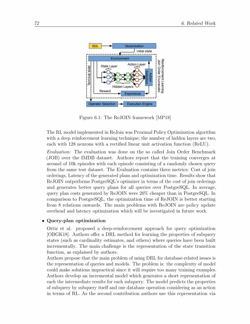
72 6. Related Work
Figure 6.1: The ReJOIN framework [MP18]
The RL model implemented in ReJoin was Proximal Policy Optimization algorithmwith a deep reinforcement learning technique; the number of hidden layers are two,each with 128 neurons with a rectified linear unit activation function (ReLU).
Evaluation: The evaluation was done on the so called Join Order Benchmark(JOB) over the IMDB dataset. Authors report that the training converges ataround of 10k episodes with each episode consisting of a randomly chosen queryfrom the same test dataset. The Evaluation contains three metrics: Cost of joinorderings, Latency of the generated plans and optimization time. Results show thatReJOIN outperforms PostgreSQL’s optimizer in terms of the cost of join orderingsand generates better query plans for all queries over PostgreSQL. In average,query plan costs generated by ReJOIN were 20% cheaper than in PostgreSQL. Incomparison to PostgreSQL, the optimization time of ReJOIN is better startingfrom 8 relations onwards. The main problems with ReJOIN are policy updateoverhead and latency optimization which will be investigated in future work.
• Query-plan optimization
Ortiz et al. proposed a deep-reinforcement approach for query optimization[OBGK18]. Authors offer a DRL method for learning the properties of subquerystates (such as cardinality estimates, and others) where queries have been builtincrementally. The main challenge is the representation of the state transitionfunction, as explained by authors.Authors propose that the main problem of using DRL for database-related issues isthe representation of queries and models. The problem is: the complexity of modelcould make solutions impractical since it will require too many training examples.Authors develop an incremental model which generates a short representation ofeach the intermediate results for each subquery. The model predicts the propertiesof subquery by subquery itself and one database operation considering as an actionin terms of RL. As the second contribution authors use this representation via
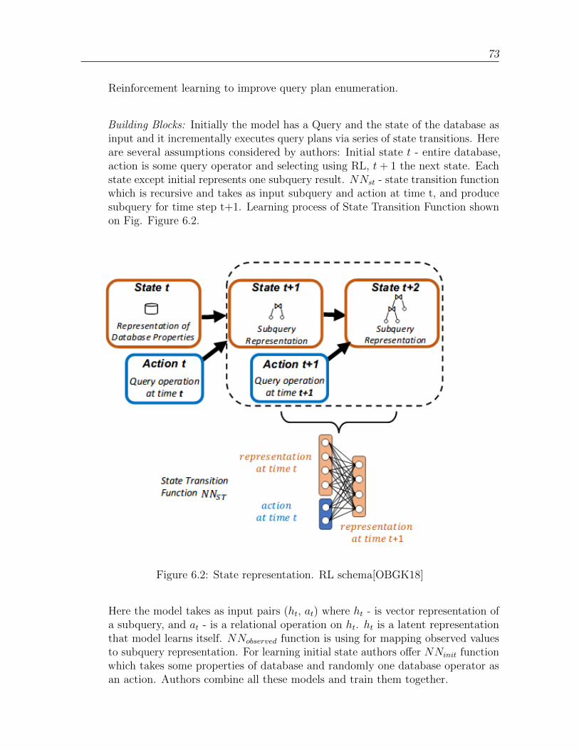
73
Reinforcement learning to improve query plan enumeration.
Building Blocks: Initially the model has a Query and the state of the database asinput and it incrementally executes query plans via series of state transitions. Hereare several assumptions considered by authors: Initial state t - entire database,action is some query operator and selecting using RL, t+ 1 the next state. Eachstate except initial represents one subquery result. NNst - state transition functionwhich is recursive and takes as input subquery and action at time t, and producesubquery for time step t+1. Learning process of State Transition Function shownon Fig. Figure 6.2.
Figure 6.2: State representation. RL schema[OBGK18]
Here the model takes as input pairs (ht, at) where ht - is vector representation ofa subquery, and at - is a relational operation on ht. ht is a latent representationthat model learns itself. NNobserved function is using for mapping observed valuesto subquery representation. For learning initial state authors offer NNinit functionwhich takes some properties of database and randomly one database operator asan action. Authors combine all these models and train them together.
74 6. Related Work
Evaluation: For evaluation authors choose the IMDB database since this databaseis more realistic and there are definitely correlation and skew between columns.As an initial experiment authors initialized x0 with properties from the IMDBdataset. As an initial action a0 authors used conjunctive selection operator.Authors generate and used 15k queries for training the model and 5k for testingpurposes. The solution contains 50 hidden nodes for one hidden layer. Authorsused Stochastic gradient-descent based algorithm for optimization, and a learningrate of 0.01. Authors compared the cardinality estimation with the value fromSQL Server. Results show that in case of 3 columns (m=3) there are heavy errorsin short epochs (less than 3) but their approach starts out-performing SQL server’sestimation after 6th epochs only. There is an observation that in case of increasingthe number of columns convergence will happen slowly. But even in that case it isshown to outperform SQL Server on the 9th epoch.
With this we conclude our review of related work in applying deep reinforcement learningto database tasks.
7. Conclusion and Future work
In this chapter, we summarize results of this thesis and give directions for furtherresearch.
7.1 Conclusion
In this work we introduced an early approach for using state-of-the art DRL methods forthe database vertical partitioning task. As a benchmark we used the TPC-H workbench.Our main contributions are:
1. Adaptation and unification of four traditional learning algorithms of verticalpartitioning, REST interface between learning RL models and these algorithms
2. Implementation and design of our own RL environment
3. Design of suitable reward function, proper action representation
4. Adaptation and integration of three existing RL agents (DQN, Rainbow, Implicitquantile) from Dopamine framework for the given task.
5. Test combination of different hyper-parameters during the training process, andevaluation of the inference process.
6. Validation of the feasibility of the current approach, though questions remain abouttwo core issues: making the inference process more competitive, and scaling-up totraining over a larger amount of workloads.
7. Discussed evaluation results
8. Brief discussion of recent works applying RL methods for database optimizationproblems.
76 7. Conclusion and Future work
We proposed two research questions. In the first we tested how learning models convergeconsidering three different case scenarios. According to our evaluation for the case 1.a(single table single workload) the iterations needed for convergence strictly depend fromthe number of steps needing to get final partition. We found that Implicit Quantileagent shows better results in terms of convergence. In case 1.b (mixed pair of tables andworkloads) we tested several hyper-parameters. We only found reasonable improvementsin terms of convergence while we use the action pruning heuristic. For the otherhyper-parameters convergence happens relatively similar despite slightly better resultsnoticeable in case of update horizon = 3, ε-greedy, and soft-update combinations. Hereagain, Implicit Quantile agent outperforms DQN and Rainbow agents.
In the most complex case 1.c (single table, random workload) we tested only one case(CUSTOMER table with random workloads) using Implicit quantile agent since this caseis much harder in comparison to previous two cases and we choose the best combinationsof hyper-parameters from previous cases. Unfortunately, we did not reach absoluteconvergence in this case and this case needs additional investigation.
Our second research question was dedicated to inference. We found that in most casesthe solutions of algorithms following a “Top-down” approach were less efficient than thoseof algorithms following a “Bottom-up” approach. This could be partly caused by theworkload itself, which could favor columnar approaches, making bottom up approachesstart from a better position. Since, our learning agents follows HillClimb algorithm asan expert, the cost is the same as in HillClimb. Also, generated partitions were shownto be the same as HillClimb, and the same as the optimal.
7.1.1 Threats to validity
• Non-machine-learning algorithms
These algorithms are available as an open-source project [JPPD] therefore theirimplementation could contain some minor bugs. During our implementation wefixed several of them (i.e., mostly in the implementation of optimal) but there arealways possibility that we miss some bugs.
• Simplification in non-machine-learning algorithms
In our experiments we considered algorithms with unified settings. Since we donot differentiate between projection and selection queries our result partitionscould be different in case of these query types will be considered. This is alsotrue regarding data replication as well as data granularity. We use meta-data ofTPC-H workbench, but in real DBMS we need to consider effect of File system,database blocks and other characteristics of real database systems.
• Heuristics regarding pruning actions
For the fast convergence, we made a heuristic of pruning actions. Despite withoutpruning of actions our models also able to converge but it took 2 times moreiterations. We are not able to prove if it is correct to use this pruning techniqueor this could considering as a bias.
7.2. Future work 77
7.2 Future work
In this thesis we show feasibility of applying RL based methods for Database verticalpartitioning optimization task. But we need to admit that we do a lot of unifications,simplifications and at the current stage the results of our research is not practical.Therefore, we need to extend this research in the several directions:
• Dedicated study for generalization
As shown, training over a stream of randomly generated cases is a big challengefor our agents. As future work, this needs to be studied with care, assessing theprecise limits of the current DRL models with regards to their ability to learn forgeneral cases, and how this aspect could be enhanced by different techniques.
• Performance improvements to inference process
In our study we report inference times that are competitive with the traditionalalgorithms, but only manage to outperform some of them for large tables. Furtheroptimization to the inference process (which apart from inference encompassesstate transitions and initialization) is highly relevant to create a more competitivesolution.
• Better reward engineering
In our implementation we need an “expert” algorithm’s best value and actionsequences for calculation reward on each step. This means that we tightly dependon expert algorithm. As a future we could consider to avoid this “expert” help,perhaps we could chose a static configuration as a baseline for normalization.
• Other RL approaches
In our research we employed value-based DRL algorithms offered by Dopamine. Butprobably, for the given task policy-based approaches are more suitable. Thereforefor a future we could employ agents based on Policy gradient methods (DPPO,TRPO etc.). Similarly, DRL algorithms for large discrete action spaces would beworthwhile to study.
• Deep learning and better feature representation
In our work we tightly rely on the NN architecture offered by Dopamine framework.Since offered convolutional NN works better for the image input, research could becontinue in the direction of choosing more suitable network structures like recurrentand recursive networks (RNN) for a given problem. Also correctly selected featuresand hyper-parameters could make the model more stable and universal.
• Integration with real world DBMS system
RL introduces new possibilities for DBMSs to expose their design and internalsto learning models. Action engineering is required to decide on the granularity,

78 7. Conclusion and Future work
the learning goal, and the way in which RL can be leveraged for DBMS design.This is a specially pertinent research area for self-driving database designs. Morespecialized open questions, pertaining to each optimization problem could beconsidered.
A. Structural views of using agents,derived from Tensorboard
Here we place schematic overviews of the used RL agents, which we derived fromTensorboard.

80 A. Structural views of using agents, derived from Tensorboard
Fig
ure
A.1
:D
QN
agen
t,st
ruct
ura
lvie
wder
ived
from
Ten
sorb
oard
.
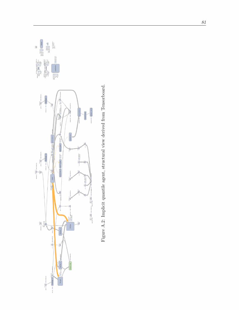
81
Fig
ure
A.2
:Im
plici
tquan
tile
agen
t,st
ruct
ura
lvie
wder
ived
from
Ten
sorb
oard
.
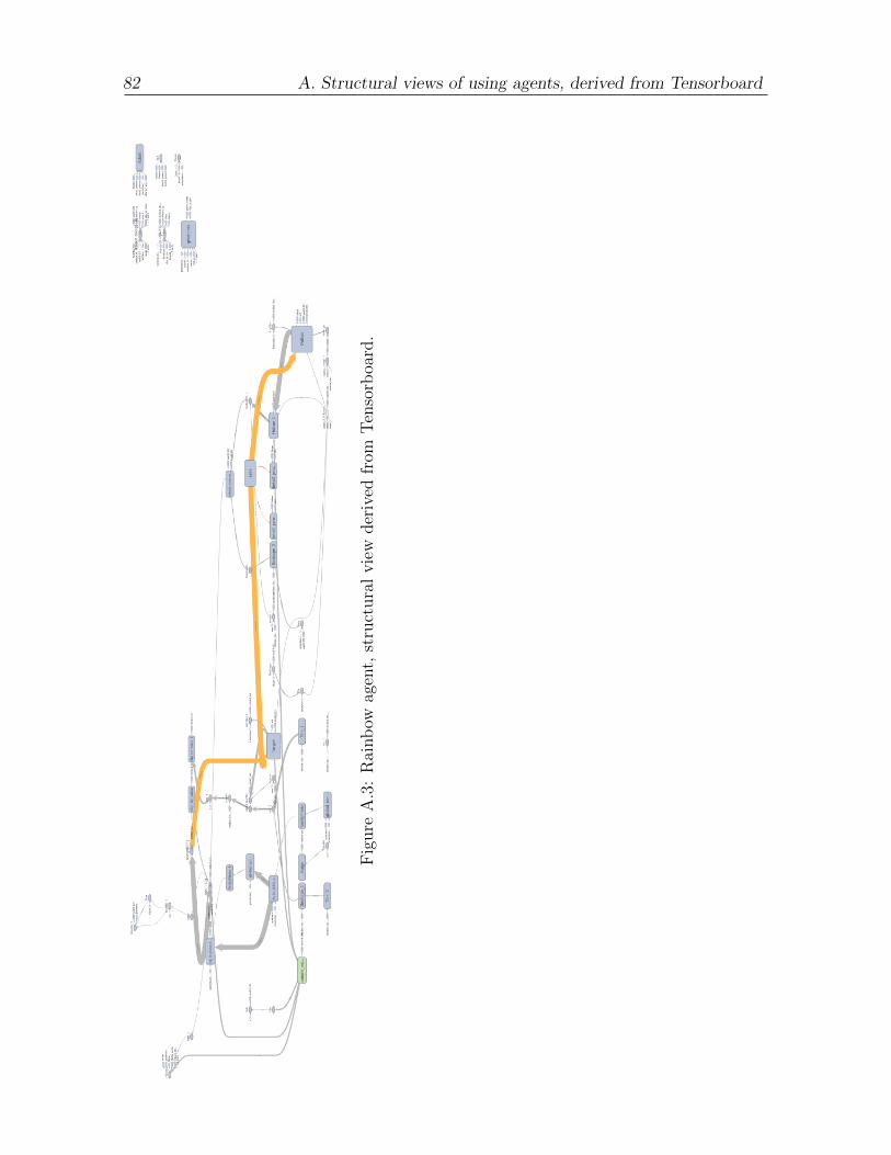
82 A. Structural views of using agents, derived from Tensorboard
Fig
ure
A.3
:R
ainb
owag
ent,
stru
ctura
lvie
wder
ived
from
Ten
sorb
oard
.
B. Hyper-parameters used for eachagent
In this section we provide hyper-parameters used for each agent during learning. InDopamine these parameters are configurable and storing in .gin template files. Majorityof used parameters provided by Dopamine and used as default.
B.1 DQN agent parameters
# Hyperparameters follow Dabney et al. (2018), but we modify as necessary to
# match those used in Rainbow (Hessel et al., 2018), to ensure apples-to-
apples
# comparison.
import gin.tf.external_configurables
DQNAgent.gamma = 0.99
DQNAgent.min_replay_history = 2000 # agent steps
DQNAgent.update_period = 4
DQNAgent.target_update_period = 1 # agent steps, was 400
DQNAgent.epsilon_train = 0.01
DQNAgent.epsilon_eval = 0.0
DQNAgent.epsilon_decay_period = 1000000 # agent steps
DQNAgent.tf_device = ’/gpu:0’ # use ’/gpu:*’ for non-GPU version
DQNAgent.optimizer = @tf.train.RMSPropOptimizer()
DQNAgent.learning_from_demo = False
tf.train.RMSPropOptimizer.learning_rate = 0.0000625
tf.train.RMSPropOptimizer.decay = 0.0
tf.train.RMSPropOptimizer.momentum = 0.0
tf.train.RMSPropOptimizer.epsilon = 0.00015
tf.train.RMSPropOptimizer.centered = True
84 B. Hyper-parameters used for each agent
WrappedReplayBufferLocal.replay_capacity = 1000000
WrappedReplayBufferLocal.batch_size = 32
run_experiment.Runner.game_name = ’GridFormationEnvSimple-v0’
# Sticky actions with probability 0.25, as suggested by (Machado et al., 2017).
run_experiment.Runner.sticky_actions = False
run_experiment.Runner.training_steps = 1000 # agent steps
run_experiment.Runner.evaluation_steps = 200 # agent steps
run_experiment.Runner.max_steps_per_episode = 25 # agent steps
run_experiment.Runner.num_iterations = 1000
B.2 Implicit Quantile agent parameters
# Hyperparameters follow Dabney et al. (2018), but we modify as necessary to
# match those used in Rainbow (Hessel et al., 2018), to ensure apples-to-
apples
# comparison.
import gin.tf.external_configurables
IQ.kappa = 1.0
IQ.num_tau_samples = 64
IQ.num_tau_prime_samples = 64
IQ.num_quantile_samples = 32
RainbowAgent.num_atoms = 51
RainbowAgent.vmax = 200.
RainbowAgent.gamma = 0.99
RainbowAgent.update_horizon = 3
RainbowAgent.min_replay_history = 2000 # agent steps
RainbowAgent.update_period = 4
RainbowAgent.target_update_period = 1 # agent steps, was 400
RainbowAgent.epsilon_train = 0.01
RainbowAgent.epsilon_eval = 0.0
RainbowAgent.epsilon_decay_period = 1000000 # agent steps
# IQN currently does not support prioritized replay.
RainbowAgent.replay_scheme = ’uniform’
RainbowAgent.tf_device = ’/gpu:0’ # use ’/cpu:*’ for non-GPU version
RainbowAgent.optimizer = @tf.train.AdamOptimizer()
IQ.learning_from_demo = False
IQ.boltzmann=False
IQ.prune_actions=True
# Note these parameters are different from C51’s.
tf.train.AdamOptimizer.learning_rate = 0.0000625
tf.train.AdamOptimizer.epsilon = 0.00015
WrappedPrioritizedReplayBufferLocal.replay_capacity = 10000
WrappedPrioritizedReplayBufferLocal.batch_size = 32
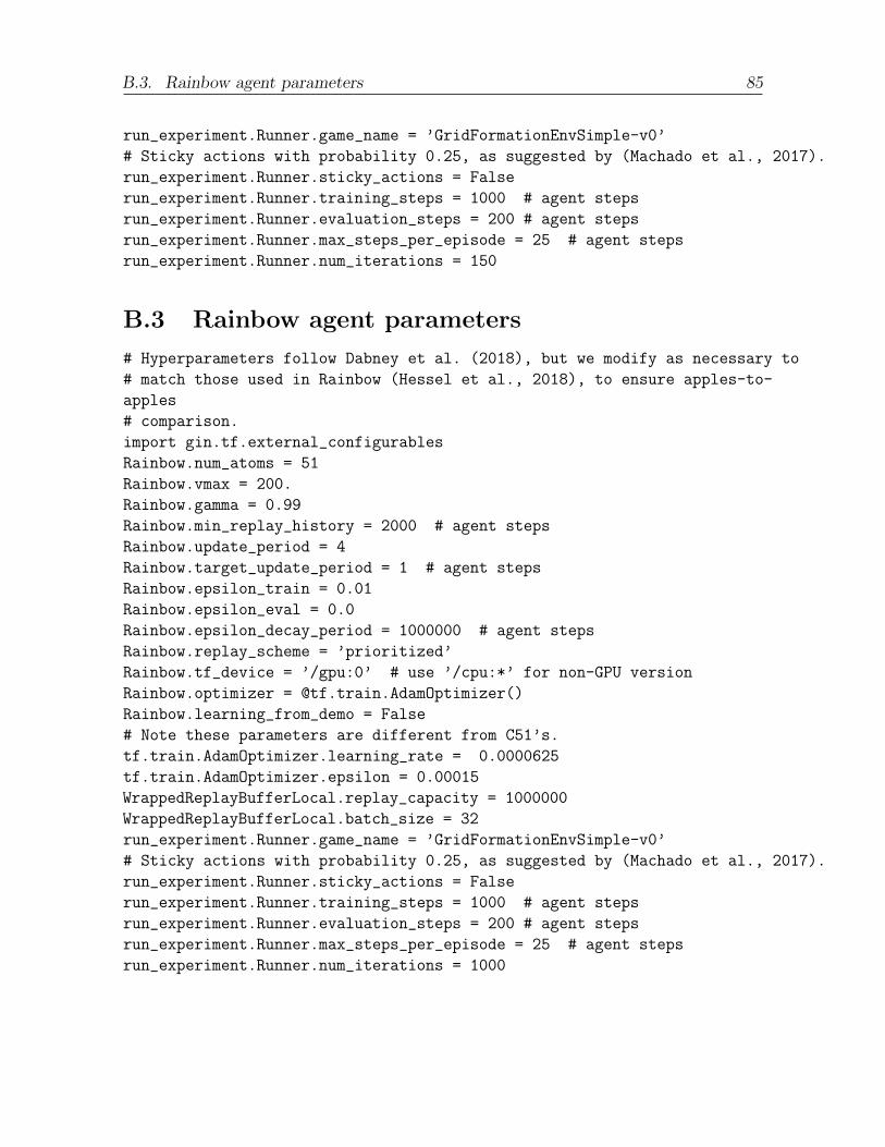
B.3. Rainbow agent parameters 85
run_experiment.Runner.game_name = ’GridFormationEnvSimple-v0’
# Sticky actions with probability 0.25, as suggested by (Machado et al., 2017).
run_experiment.Runner.sticky_actions = False
run_experiment.Runner.training_steps = 1000 # agent steps
run_experiment.Runner.evaluation_steps = 200 # agent steps
run_experiment.Runner.max_steps_per_episode = 25 # agent steps
run_experiment.Runner.num_iterations = 150
B.3 Rainbow agent parameters
# Hyperparameters follow Dabney et al. (2018), but we modify as necessary to
# match those used in Rainbow (Hessel et al., 2018), to ensure apples-to-
apples
# comparison.
import gin.tf.external_configurables
Rainbow.num_atoms = 51
Rainbow.vmax = 200.
Rainbow.gamma = 0.99
Rainbow.min_replay_history = 2000 # agent steps
Rainbow.update_period = 4
Rainbow.target_update_period = 1 # agent steps
Rainbow.epsilon_train = 0.01
Rainbow.epsilon_eval = 0.0
Rainbow.epsilon_decay_period = 1000000 # agent steps
Rainbow.replay_scheme = ’prioritized’
Rainbow.tf_device = ’/gpu:0’ # use ’/cpu:*’ for non-GPU version
Rainbow.optimizer = @tf.train.AdamOptimizer()
Rainbow.learning_from_demo = False
# Note these parameters are different from C51’s.
tf.train.AdamOptimizer.learning_rate = 0.0000625
tf.train.AdamOptimizer.epsilon = 0.00015
WrappedReplayBufferLocal.replay_capacity = 1000000
WrappedReplayBufferLocal.batch_size = 32
run_experiment.Runner.game_name = ’GridFormationEnvSimple-v0’
# Sticky actions with probability 0.25, as suggested by (Machado et al., 2017).
run_experiment.Runner.sticky_actions = False
run_experiment.Runner.training_steps = 1000 # agent steps
run_experiment.Runner.evaluation_steps = 200 # agent steps
run_experiment.Runner.max_steps_per_episode = 25 # agent steps
run_experiment.Runner.num_iterations = 1000

86 B. Hyper-parameters used for each agent
C. Inference times
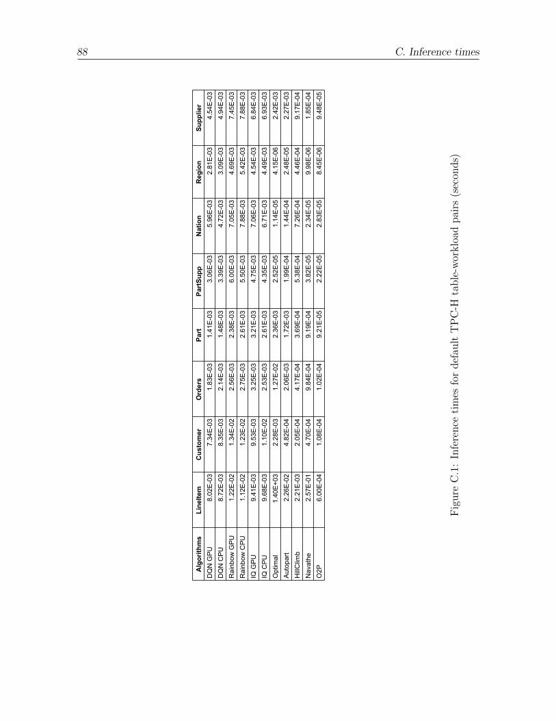
88 C. Inference times
Algorith
ms
LineItem
Customer
Orders
Part
PartSu
ppNation
Region
Supp
lier
DQ
N G
PU
8.02
E-0
37.
34E
-03
1.83
E-0
31.
41E
-03
3.06
E-0
35.
96E
-03
2.81
E-0
34.
54E
-03
DQ
N C
PU
8.72
E-0
38.
35E
-03
2.14
E-0
31.
48E
-03
3.39
E-0
34.
72E
-03
3.09
E-0
34.
94E
-03
Rai
nbow
GP
U1.
22E
-02
1.34
E-0
22.
56E
-03
2.38
E-0
36.
00E
-03
7.05
E-0
34.
69E
-03
7.45
E-0
3R
ainb
ow C
PU
1.12
E-0
21.
23E
-02
2.75
E-0
32.
61E
-03
5.50
E-0
37.
88E
-03
5.42
E-0
37.
88E
-03
IQ G
PU
9.41
E-0
39.
53E
-03
3.25
E-0
33.
21E
-03
4.75
E-0
37.
06E
-03
4.54
E-0
36.
84E
-03
IQ C
PU
9.68
E-0
31.
10E
-02
2.53
E-0
32.
61E
-03
4.35
E-0
36.
71E
-03
4.49
E-0
36.
93E
-03
Opt
imal
1.40
E+0
32.
28E
-03
1.27
E-0
22.
36E
-03
2.52
E-0
51.
14E
-05
4.15
E-0
62.
42E
-03
Aut
opar
t2.
26E
-02
4.82
E-0
42.
06E
-03
1.72
E-0
31.
99E
-04
1.44
E-0
42.
48E
-05
2.27
E-0
3H
illC
limb
2.21
E-0
32.
05E
-04
4.17
E-0
43.
69E
-04
5.38
E-0
47.
26E
-04
4.46
E-0
49.
17E
-04
Nav
athe
2.57
E-0
14.
70E
-04
9.84
E-0
49.
19E
-04
3.82
E-0
52.
34E
-05
9.98
E-0
61.
85E
-04
O2P
6.00
E-0
41.
08E
-04
1.02
E-0
49.
21E
-05
2.22
E-0
52.
83E
-05
8.45
E-0
69.
48E
-05
Fig
ure
C.1
:In
fere
nce
tim
esfo
rdef
ault
TP
C-H
table
-wor
klo
adpai
rs(s
econ
ds)
Bibliography
[72] Problem decomposition and data reorganization by a clustering technique.Oper. Res., 20(5):993–1009, October 1972. (cited on Page xi, 14, and 15)
[ABCN06] Sanjay Agrawal, Nicolas Bruno, Surajit Chaudhuri, and Vivek RNarasayya. Autoadmin: Self-tuning database systemstechnology. IEEEData Eng. Bull., 29(3):7–15, 2006. (cited on Page 2)
[ANY04a] Sanjay Agrawal, Vivek Narasayya, and Beverly Yang. Integrating verticaland horizontal partitioning into automated physical database design.In Proceedings of the 2004 ACM SIGMOD international conference onManagement of data, pages 359–370. ACM, 2004. (cited on Page 11)
[ANY04b] Sanjay Agrawal, Vivek R. Narasayya, and Beverly Yang. Integratingvertical and horizontal partitioning into automated physical databasedesign. In SIGMOD Conference, 2004. (cited on Page iii)
[Ape88] Peter M. G. Apers. Data allocation in distributed database systems. ACMTrans. Database Syst., 13:263–304, 1988. (cited on Page 12)
[BAA12a] Renata Borovica, Ioannis Alagiannis, and Anastasia Ailamaki. Automatedphysical designers: What you see is (not) what you get. In Proceedings ofthe Fifth International Workshop on Testing Database Systems, DBTest’12, pages 9:1–9:6, New York, NY, USA, 2012. ACM. (cited on Page iii)
[BAA12b] Renata Borovica, Ioannis Alagiannis, and Anastasia Ailamaki. Automatedphysical designers: what you see is (not) what you get. In Proceedings ofthe Fifth International Workshop on Testing Database Systems, page 9.ACM, 2012. (cited on Page 2)
[BDM17] Marc G. Bellemare, Will Dabney, and Remi Munos. A distributionalperspective on reinforcement learning. CoRR, abs/1707.06887, 2017.(cited on Page 29)
[Bel09] Ladjel Bellatreche. Optimization and Tuning in Data Warehouses, pages1995–2003. Springer US, Boston, MA, 2009. (cited on Page iii)
90 Bibliography
[BLC+15] Debabrota Basu, Qian Lin, Weidong Chen, Hoang Tam Vo, Zihong Yuan,Pierre Senellart, and Stephane Bressan. Cost-model oblivious databasetuning with reinforcement learning. In Proceedings, Part I, of the 26thInternational Conference on Database and Expert Systems Applications -Volume 9261, DEXA 2015, pages 253–268, 2015. (cited on Page 69)
[BNVB13] Marc G Bellemare, Yavar Naddaf, Joel Veness, and Michael Bowling. Thearcade learning environment: An evaluation platform for general agents.Journal of Artificial Intelligence Research, 47:253–279, 2013. (cited on
Page 4)
[CMG+18] Pablo Samuel Castro, Subhodeep Moitra, Carles Gelada, Saurabh Kumar,and Marc G Bellemare. Dopamine: A research framework for deepreinforcement learning. arXiv preprint arXiv:1812.06110, 2018. (cited on
Page 4 and 34)
[CY90] D. Cornell and P. Yu. An effective approach to vertical partitioning forphysical design of relational databases. IEEE Transactions on SoftwareEngineering, 16:248–258, 02 1990. (cited on Page 11)
[DAEvH+15] Gabriel Dulac-Arnold, Richard Evans, Hado van Hasselt, Peter Sunehag,Timothy Lillicrap, Jonathan Hunt, Timothy Mann, Theophane Weber,Thomas Degris, and Ben Coppin. Deep reinforcement learning in largediscrete action spaces. arXiv preprint arXiv:1512.07679, 2015. (cited on
Page 4)
[DHJ+07] Giuseppe DeCandia, Deniz Hastorun, Madan Jampani, GunavardhanKakulapati, Avinash Lakshman, Alex Pilchin, Swaminathan Sivasubra-manian, Peter Vosshall, and Werner Vogels. Dynamo: amazon’s highlyavailable key-value store. In ACM SIGOPS operating systems review,volume 41, pages 205–220. ACM, 2007. (cited on Page 10)
[DOSM18] Will Dabney, Georg Ostrovski, David Silver, and Remi Munos. Im-plicit quantile networks for distributional reinforcement learning. CoRR,abs/1806.06923, 2018. (cited on Page xi, 29, and 30)
[DPP+18] Gabriel Campero Durand, Marcus Pinnecke, Rufat Piriyev, MahmoudMohsen, David Broneske, Gunter Saake, Maya S Sekeran, Fabian Ro-driguez, and Laxmi Balami. Gridformation: Towards self-driven onlinedata partitioning using reinforcement learning. In Proceedings of the FirstInternational Workshop on Exploiting Artificial Intelligence Techniquesfor Data Management, page 1. ACM, 2018. (cited on Page 69)
[DY+14] Li Deng, Dong Yu, et al. Deep learning: methods and applications.Foundations and Trends R© in Signal Processing, 7(3–4):197–387, 2014.(cited on Page 25)
Bibliography 91
[FLHI+18] Vincent Francois-Lavet, Peter Henderson, Riashat Islam, Marc G Belle-mare, Joelle Pineau, et al. An introduction to deep reinforcement learning.Foundations and Trends R© in Machine Learning, 11(3-4):219–354, 2018.(cited on Page 3 and 24)
[GCNG16] Vyacheslav Galaktionov, George Chernishev, Boris Novikov, and DmitryGrigoriev. Matrix clustering algorithms for vertical partitioning problem:an initial performance study. In DAMDID/RCDL, 2016. (cited on Page iii
and 12)
[HGS16] Hado van Hasselt, Arthur Guez, and David Silver. Deep reinforcementlearning with double q-learning. In Proceedings of the Thirtieth AAAIConference on Artificial Intelligence, AAAI’16, pages 2094–2100. AAAIPress, 2016. (cited on Page 28)
[HMvH+17] Matteo Hessel, Joseph Modayil, Hado van Hasselt, Tom Schaul, GeorgOstrovski, Will Dabney, Daniel Horgan, Bilal Piot, Mohammad GheshlaghiAzar, and David Silver. Rainbow: Combining improvements in deepreinforcement learning. CoRR, abs/1710.02298, 2017. (cited on Page 30)
[HN79a] Michael Hammer and Bahram Niamir. A heuristic approach to attributepartitioning. In Proceedings of the 1979 ACM SIGMOD InternationalConference on Management of Data, SIGMOD ’79, pages 93–101, NewYork, NY, USA, 1979. ACM. (cited on Page 2)
[HN79b] Michael Hammer and Bahram Niamir. A heuristic approach to attributepartitioning., 01 1979. (cited on Page 11)
[HP03] Richard A. Hankins and Jignesh M. Patel. Data morphing: An adaptive,cache-conscious storage technique. In VLDB, 2003. (cited on Page 13
and 19)
[JD12] Alekh Jindal and Jens Dittrich. Relax and let the database do thepartitioning online. In Malu Castellanos, Umeshwar Dayal, and WolfgangLehner, editors, Enabling Real-Time Business Intelligence, pages 65–80,Berlin, Heidelberg, 2012. Springer Berlin Heidelberg. (cited on Page 11, 13,
and 16)
[JPPD] Alekh Jindal, Endre Palatinus, Vladimir Pavlov, and Jens Dittrich. Acomparison of knives for bread slicing. (cited on Page iii, 2, 4, 11, 12, 14, 33,
37, 39, 65, and 76)
[JQRD11] Alekh Jindal, Jorge-Arnulfo Quiane-Ruiz, and Jens Dittrich. Trojan datalayouts: Right shoes for a running elephant. In Proceedings of the 2NdACM Symposium on Cloud Computing, SOCC ’11, pages 21:1–21:14, NewYork, NY, USA, 2011. ACM. (cited on Page iii and 13)
92 Bibliography
[KBCG18] Tomer Kaftan, Magdalena Balazinska, Alvin Cheung, and JohannesGehrke. Cuttlefish: A lightweight primitive for adaptive query processing.CoRR, abs/1802.09180, 2018. (cited on Page 69)
[KS86] Henry F. Korth and Abraham Silberschatz. Database System Concepts.McGraw-Hill, Inc., New York, NY, USA, 1986. (cited on Page 1 and 10)
[Loh14] Guy Lohman. Is query optimization a“solved”problem. In Proc. Workshopon Database Query Optimization, page 13. Oregon Graduate Center Comp.Sci. Tech. Rep, 2014. (cited on Page 2)
[MKS+13] Volodymyr Mnih, Koray Kavukcuoglu, David Silver, Alex Graves, IoannisAntonoglou, Daan Wierstra, and Martin Riedmiller. Playing atari withdeep reinforcement learning. In NIPS Deep Learning Workshop. 2013.(cited on Page 27 and 28)
[MKS+15] Volodymyr Mnih, Koray Kavukcuoglu, David Silver, Andrei A. Rusu, JoelVeness, Marc G. Bellemare, Alex Graves, Martin Riedmiller, Andreas K.Fidjeland, Georg Ostrovski, Stig Petersen, Charles Beattie, Amir Sadik,Ioannis Antonoglou, Helen King, Dharshan Kumaran, Daan Wierstra,Shane Legg, and Demis Hassabis. Human-level control through deepreinforcement learning. Nature, 518(7540):529–533, 02 2015. (cited on
Page 27)
[MP18] Ryan Marcus and Olga Papaemmanouil. Deep reinforcement learning forjoin order enumeration. In Proceedings of the First International Workshopon Exploiting Artificial Intelligence Techniques for Data Management,page 3. ACM, 2018. (cited on Page xii, 69, 71, and 72)
[NCWD84a] Shamkant Navathe, Stefano Ceri, Gio Wiederhold, and Jinglie Dou. Ver-tical partitioning algorithms for database design. ACM Transactions onDatabase Systems, 9:680–710, 1984. (cited on Page 9, 10, 13, and 14)
[NCWD84b] Shamkant Navathe, Stefano Ceri, Gio Wiederhold, and Jinglie Dou. Verti-cal partitioning algorithms for database design. ACM Trans. DatabaseSyst., 9(4):680–710, December 1984. (cited on Page 11 and 13)
[OBGK18] Jennifer Ortiz, Magdalena Balazinska, Johannes Gehrke, and S SathiyaKeerthi. Learning state representations for query optimization with deepreinforcement learning. In Proceedings of the Second Workshop on DataManagement for End-To-End Machine Learning, page 4. ACM, 2018.(cited on Page xii, 69, 72, and 73)
[PA04a] S. Papadomanolakis and A. Ailamaki. Autopart: automating schemadesign for large scientific databases using data partitioning. In Proceed-ings. 16th International Conference on Scientific and Statistical DatabaseManagement, 2004., pages 383–392, June 2004. (cited on Page xi, 13, 18,
and 19)
Bibliography 93
[PA04b] Stratos Papadomanolakis and Anastassia Ailamaki. Autopart: Automat-ing schema design for large scientific databases using data partitioning.In Proceedings of the 16th International Conference on Scientific andStatistical Database Management, SSDBM ’04, pages 383–, Washington,DC, USA, 2004. IEEE Computer Society. (cited on Page 11, 13, and 18)
[PAA+17] Andrew Pavlo, Gustavo Angulo, Joy Arulraj, Haibin Lin, Jiexi Lin, LinMa, Prashanth Menon, Todd C Mowry, Matthew Perron, Ian Quah, et al.Self-driving database management systems. In CIDR, 2017. (cited on
Page 2)
[SB98] Richard S. Sutton and Andrew G. Barto. Introduction to ReinforcementLearning. MIT Press, Cambridge, MA, USA, 1st edition, 1998. (cited on
Page 21, 23, and 24)
[SQAS15] Tom Schaul, John Quan, Ioannis Antonoglou, and David Silver. Prioritizedexperience replay. CoRR, abs/1511.05952, 2015. (cited on Page 28)
[SSD18] Ankur Sharma, Felix Martin Schuhknecht, and Jens Dittrich. The casefor automatic database administration using deep reinforcement learning.ArXiv e-prints, January 2018. (cited on Page 69 and 70)
[SW85] Domenico Sacca and Gio Wiederhold. Database partitioning in a cluster ofprocessors. ACM Transactions on Database Systems (TODS), 10(1):29–56,1985. (cited on Page 10)
[TSJ08] Kostas Tzoumas, Timos Sellis, and Christian S Jensen. A reinforcementlearning approach for adaptive query processing. History, 2008. (cited on
Page 69)
[VAPGZ17] Dana Van Aken, Andrew Pavlo, Geoffrey J Gordon, and Bohan Zhang.Automatic database management system tuning through large-scale ma-chine learning. In Proceedings of the 2017 ACM International Conferenceon Management of Data, pages 1009–1024. ACM, 2017. (cited on Page 2)
[WD92] Christopher J. C. H. Watkins and Peter Dayan. Q-learning. MachineLearning, 8(3):279–292, May 1992. (cited on Page 24)
[Wir00] Rudiger Wirth. Crisp-dm: Towards a standard process model for datamining. In Proceedings of the Fourth International Conference on thePractical Application of Knowledge Discovery and Data Mining, pages29–39, 2000. (cited on Page 5)

94 Bibliography