Self-Driving Cars: Evaluation of Deep Learning Techniques

SMU Data Science Review

Volume 2 | Number 1 Article 23

2019

Self-Driving Cars: Evaluation of Deep LearningTechniques for Object Detection in DifferentDriving ConditionsRamesh SimhambhatlaSMU, [email protected]

Kevin OkiahSMU, [email protected]

Shravan KuchkulaSMU, [email protected]

Robert SlaterSouthern Methodist University, [email protected]

Follow this and additional works at: https://scholar.smu.edu/datasciencereview

Part of the Artificial Intelligence and Robotics Commons, Other Computer EngineeringCommons, and the Statistical Models Commons

This Article is brought to you for free and open access by SMU Scholar. It has been accepted for inclusion in SMU Data Science Review by anauthorized administrator of SMU Scholar. For more information, please visit http://digitalrepository.smu.edu.

Recommended CitationSimhambhatla, Ramesh; Okiah, Kevin; Kuchkula, Shravan; and Slater, Robert (2019) "Self-Driving Cars: Evaluation of Deep LearningTechniques for Object Detection in Different Driving Conditions," SMU Data Science Review: Vol. 2 : No. 1 , Article 23.Available at: https://scholar.smu.edu/datasciencereview/vol2/iss1/23

https://scholar.smu.edu/datasciencereview?utm_source=scholar.smu.edu%2Fdatasciencereview%2Fvol2%2Fiss1%2F23&utm_medium=PDF&utm_campaign=PDFCoverPages

https://scholar.smu.edu/datasciencereview/vol2?utm_source=scholar.smu.edu%2Fdatasciencereview%2Fvol2%2Fiss1%2F23&utm_medium=PDF&utm_campaign=PDFCoverPages

https://scholar.smu.edu/datasciencereview/vol2/iss1?utm_source=scholar.smu.edu%2Fdatasciencereview%2Fvol2%2Fiss1%2F23&utm_medium=PDF&utm_campaign=PDFCoverPages

https://scholar.smu.edu/datasciencereview/vol2/iss1/23?utm_source=scholar.smu.edu%2Fdatasciencereview%2Fvol2%2Fiss1%2F23&utm_medium=PDF&utm_campaign=PDFCoverPages

https://scholar.smu.edu/datasciencereview?utm_source=scholar.smu.edu%2Fdatasciencereview%2Fvol2%2Fiss1%2F23&utm_medium=PDF&utm_campaign=PDFCoverPages

http://network.bepress.com/hgg/discipline/143?utm_source=scholar.smu.edu%2Fdatasciencereview%2Fvol2%2Fiss1%2F23&utm_medium=PDF&utm_campaign=PDFCoverPages




https://scholar.smu.edu/datasciencereview/vol2/iss1/23?utm_source=scholar.smu.edu%2Fdatasciencereview%2Fvol2%2Fiss1%2F23&utm_medium=PDF&utm_campaign=PDFCoverPages

http://digitalrepository.smu.edu

Self-Driving Cars: Evaluation of Deep Learning

Techniques for Object Detection in Different Driving

Conditions

Kevin Okiah1, Shravan Kuchkula1, Ramesh Simhambhatla1, Robert Slater1

1 Master of Science in Data Science, Southern Methodist University,

Dallas, TX 75275 USA

{KOkiah, SKuchkula, RSimhambhatla, RSlater}@smu.edu

Abstract. Deep Learning has revolutionized Computer Vision, and it is the core

technology behind capabilities of a self-driving car. Convolutional Neural

Networks (CNNs) are at the heart of this deep learning revolution for improving

the task of object detection. A number of successful object detection systems

have been proposed in recent years that are based on CNNs. In this paper, an

empirical evaluation of three recent meta-architectures: SSD (Single Shot multi-

box Detector), R-CNN (Region-based CNN) and R-FCN (Region-based Fully

Convolutional Networks) was conducted to measure how fast and accurate they

are in identifying objects on the road, such as vehicles, pedestrians, traffic lights,

etc. under four different driving conditions: day, night, rainy and snowy for four

different image widths: 150, 300, 450 and 600. The results show that region-

based algorithms have higher accuracy with lower inference times for all driving

conditions and image sizes. The second principle contribution of this paper is to

show that Transfer Learning can be an effective paradigm in improving the

performance of these pre-trained networks. With Transfer Learning, we were

able to improve the accuracy for rainy and night conditions and achieve less

than 2 seconds per image inference time for all conditions, which outperformed

the pre-trained networks.

1 Introduction

Computer Vision has become increasingly important and effective in recent years due

to its wide-ranging applications in areas as diverse as smart surveillance and

monitoring, health and medicine, sports and recreation, robotics, drones, and self-

driving cars. Visual recognition tasks, such as image classification, localization, and

detection, are the core building blocks of many of these applications and recent

developments in Convolutional Neural Networks (CNNs) have led to outstanding

performance in these state-of-the-art visual recognition tasks and systems. CNNs are

primarily used for image classification tasks, such as, looking at an image and

classifying the object in it.

In contrast, the term object localization refers to the task of identifying the location

of an object in the image. An object localization algorithm will output the coordinates

of the location of an object with respect to the image. In computer vision, the most

popular way to localize an object in an image is to represent its location with the help

of bounding boxes. The task of object detection combines both classification and

localization to identify multiple objects in an image and locate each object within the

image. A well-known application of multiple object detection is in self-driving cars,

where the algorithm not only needs to detect the cars but also pedestrians,

1

Simhambhatla et al.: Self-Driving Cars: Evaluation of Deep Learning Techniques for Object Detection in Different Driving Conditions

Published by SMU Scholar, 2019

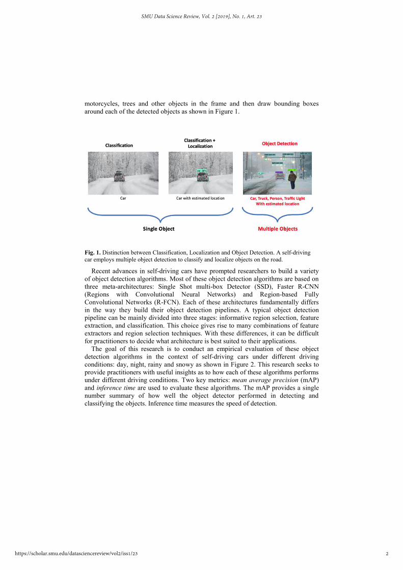
motorcycles, trees and other objects in the frame and then draw bounding boxes

around each of the detected objects as shown in Figure 1.

Fig. 1. Distinction between Classification, Localization and Object Detection. A self-driving

car employs multiple object detection to classify and localize objects on the road.

Recent advances in self-driving cars have prompted researchers to build a variety

of object detection algorithms. Most of these object detection algorithms are based on

three meta-architectures: Single Shot multi-box Detector (SSD), Faster R-CNN

(Regions with Convolutional Neural Networks) and Region-based Fully

Convolutional Networks (R-FCN). Each of these architectures fundamentally differs

in the way they build their object detection pipelines. A typical object detection

pipeline can be mainly divided into three stages: informative region selection, feature

extraction, and classification. This choice gives rise to many combinations of feature

extractors and region selection techniques. With these differences, it can be difficult

for practitioners to decide what architecture is best suited to their applications.

The goal of this research is to conduct an empirical evaluation of these object

detection algorithms in the context of self-driving cars under different driving

conditions: day, night, rainy and snowy as shown in Figure 2. This research seeks to

provide practitioners with useful insights as to how each of these algorithms performs

under different driving conditions. Two key metrics: mean average precision (mAP)

and inference time are used to evaluate these algorithms. The mAP provides a single

number summary of how well the object detector performed in detecting and

classifying the objects. Inference time measures the speed of detection.

2

SMU Data Science Review, Vol. 2 [2019], No. 1, Art. 23

https://scholar.smu.edu/datasciencereview/vol2/iss1/23

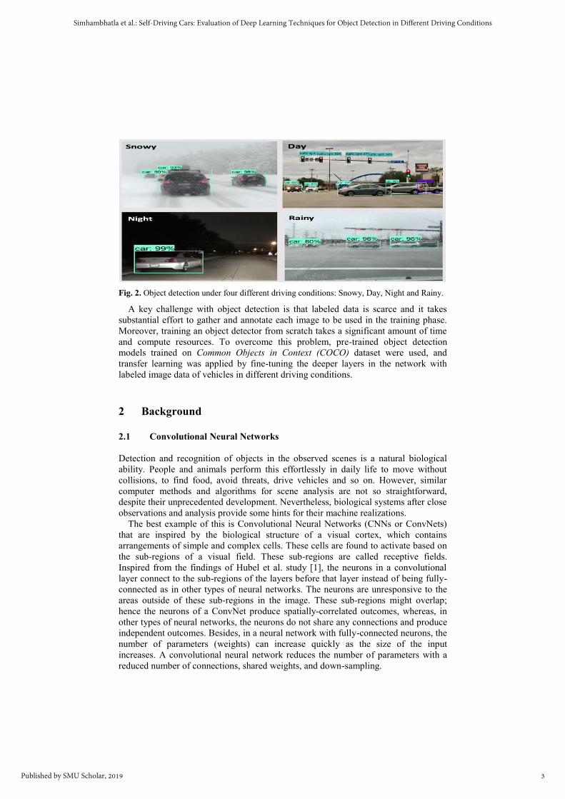
Fig. 2. Object detection under four different driving conditions: Snowy, Day, Night and Rainy.

A key challenge with object detection is that labeled data is scarce and it takes

substantial effort to gather and annotate each image to be used in the training phase.

Moreover, training an object detector from scratch takes a significant amount of time

and compute resources. To overcome this problem, pre-trained object detection

models trained on Common Objects in Context (COCO) dataset were used, and

transfer learning was applied by fine-tuning the deeper layers in the network with

labeled image data of vehicles in different driving conditions.

2 Background

2.1 Convolutional Neural Networks

Detection and recognition of objects in the observed scenes is a natural biological

ability. People and animals perform this effortlessly in daily life to move without

collisions, to find food, avoid threats, drive vehicles and so on. However, similar

computer methods and algorithms for scene analysis are not so straightforward,

despite their unprecedented development. Nevertheless, biological systems after close

observations and analysis provide some hints for their machine realizations.

The best example of this is Convolutional Neural Networks (CNNs or ConvNets)

that are inspired by the biological structure of a visual cortex, which contains

arrangements of simple and complex cells. These cells are found to activate based on

the sub-regions of a visual field. These sub-regions are called receptive fields.

Inspired from the findings of Hubel et al. study [1], the neurons in a convolutional

layer connect to the sub-regions of the layers before that layer instead of being fully-

connected as in other types of neural networks. The neurons are unresponsive to the

areas outside of these sub-regions in the image. These sub-regions might overlap;

hence the neurons of a ConvNet produce spatially-correlated outcomes, whereas, in

other types of neural networks, the neurons do not share any connections and produce

independent outcomes. Besides, in a neural network with fully-connected neurons, the

number of parameters (weights) can increase quickly as the size of the input

increases. A convolutional neural network reduces the number of parameters with a

reduced number of connections, shared weights, and down-sampling.

3



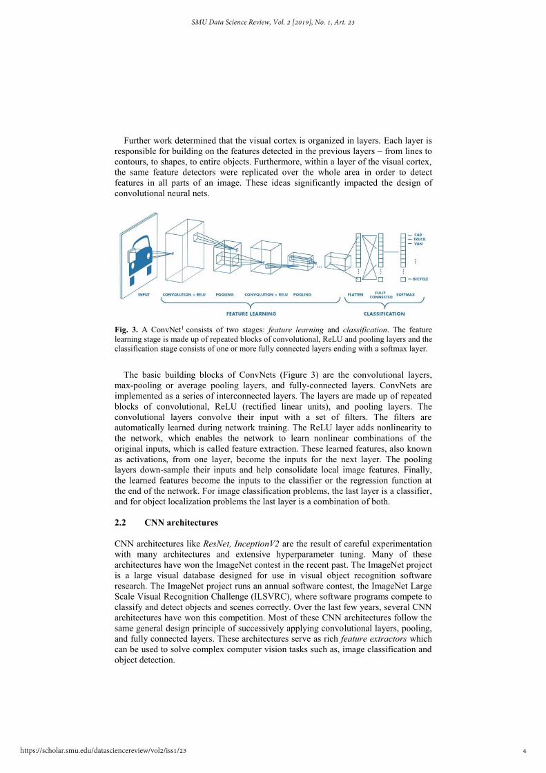
Further work determined that the visual cortex is organized in layers. Each layer is

responsible for building on the features detected in the previous layers – from lines to

contours, to shapes, to entire objects. Furthermore, within a layer of the visual cortex,

the same feature detectors were replicated over the whole area in order to detect

features in all parts of an image. These ideas significantly impacted the design of

convolutional neural nets.

Fig. 3. A ConvNet1 consists of two stages: feature learning and classification. The feature

learning stage is made up of repeated blocks of convolutional, ReLU and pooling layers and the

classification stage consists of one or more fully connected layers ending with a softmax layer.

The basic building blocks of ConvNets (Figure 3) are the convolutional layers,

max-pooling or average pooling layers, and fully-connected layers. ConvNets are

implemented as a series of interconnected layers. The layers are made up of repeated

blocks of convolutional, ReLU (rectified linear units), and pooling layers. The

convolutional layers convolve their input with a set of filters. The filters are

automatically learned during network training. The ReLU layer adds nonlinearity to

the network, which enables the network to learn nonlinear combinations of the

original inputs, which is called feature extraction. These learned features, also known

as activations, from one layer, become the inputs for the next layer. The pooling

layers down-sample their inputs and help consolidate local image features. Finally,

the learned features become the inputs to the classifier or the regression function at

the end of the network. For image classification problems, the last layer is a classifier,

and for object localization problems the last layer is a combination of both.

2.2 CNN architectures

CNN architectures like ResNet, InceptionV2 are the result of careful experimentation

with many architectures and extensive hyperparameter tuning. Many of these

architectures have won the ImageNet contest in the recent past. The ImageNet project

is a large visual database designed for use in visual object recognition software

research. The ImageNet project runs an annual software contest, the ImageNet Large

Scale Visual Recognition Challenge (ILSVRC), where software programs compete to

classify and detect objects and scenes correctly. Over the last few years, several CNN

architectures have won this competition. Most of these CNN architectures follow the

same general design principle of successively applying convolutional layers, pooling,

and fully connected layers. These architectures serve as rich feature extractors which

can be used to solve complex computer vision tasks such as, image classification and

object detection.

4



2.3 Computer Vision tasks

Computer Vision is the science of computers and software systems that can recognize

and understand images and scenes. As depicted in Figure 4, the three most common

tasks in computer vision are image classification, classification with localization and

object detection.

Fig. 4. Three most common Computer vision tasks2: classification, classification with

localization and object detection.

2.3.1 Image Classification: This is the most common computer vision problem

where an algorithm looks at an image and classifies the object in it. Image

classification has a wide variety of applications, ranging from face detection on social

networks to cancer detection in medicine. Such problems are typically modeled using

Convolutional Neural Nets (CNNs). Figure 5 shows the high-level steps involved in a

typical image classification task. The input image is sent through multiple

convolutional, pooling, non-linear layers and the output of the final layer of the CNN

is passed into a softmax layer which converts the numbers between 0 and 1, giving

the probability of the image being of a particular class.

Fig. 5. Steps for image classification using CNN1: split the image into three channels; pass it

through a series of convolutional, non-linear and pooling layers; feed this into a softmax layer.

1 https://towardsdatascience.com/evolution-of-object-detection-and-localization-algorithms-

e241021d8bad

5



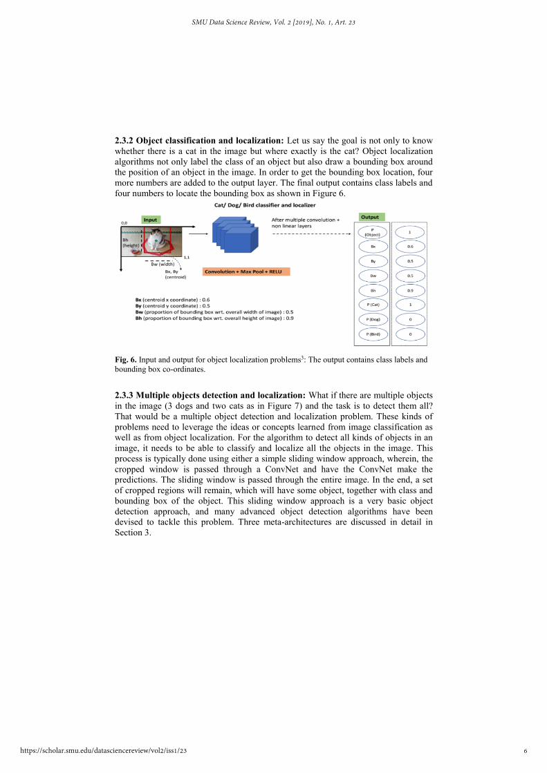
2.3.2 Object classification and localization: Let us say the goal is not only to know

whether there is a cat in the image but where exactly is the cat? Object localization

algorithms not only label the class of an object but also draw a bounding box around

the position of an object in the image. In order to get the bounding box location, four

more numbers are added to the output layer. The final output contains class labels and

four numbers to locate the bounding box as shown in Figure 6.

Fig. 6. Input and output for object localization problems3: The output contains class labels and

bounding box co-ordinates.

2.3.3 Multiple objects detection and localization: What if there are multiple objects

in the image (3 dogs and two cats as in Figure 7) and the task is to detect them all?

That would be a multiple object detection and localization problem. These kinds of

problems need to leverage the ideas or concepts learned from image classification as

well as from object localization. For the algorithm to detect all kinds of objects in an

image, it needs to be able to classify and localize all the objects in the image. This

process is typically done using either a simple sliding window approach, wherein, the

cropped window is passed through a ConvNet and have the ConvNet make the

predictions. The sliding window is passed through the entire image. In the end, a set

of cropped regions will remain, which will have some object, together with class and

bounding box of the object. This sliding window approach is a very basic object

detection approach, and many advanced object detection algorithms have been

devised to tackle this problem. Three meta-architectures are discussed in detail in

Section 3.

6



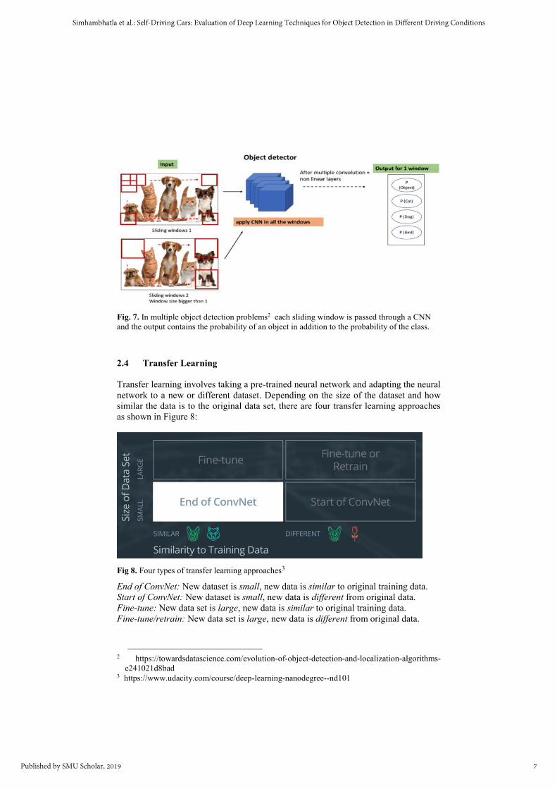
Fig. 7. In multiple object detection problems2 each sliding window is passed through a CNN

and the output contains the probability of an object in addition to the probability of the class.

2.4 Transfer Learning

Transfer learning involves taking a pre-trained neural network and adapting the neural

network to a new or different dataset. Depending on the size of the dataset and how

similar the data is to the original data set, there are four transfer learning approaches

as shown in Figure 8:

Fig 8. Four types of transfer learning approaches3

End of ConvNet: New dataset is small, new data is similar to original training data.

Start of ConvNet: New dataset is small, new data is different from original data.

Fine-tune: New data set is large, new data is similar to original training data.

Fine-tune/retrain: New data set is large, new data is different from original data.

2 https://towardsdatascience.com/evolution-of-object-detection-and-localization-algorithms-

e241021d8bad 3 https://www.udacity.com/course/deep-learning-nanodegree--nd101

7



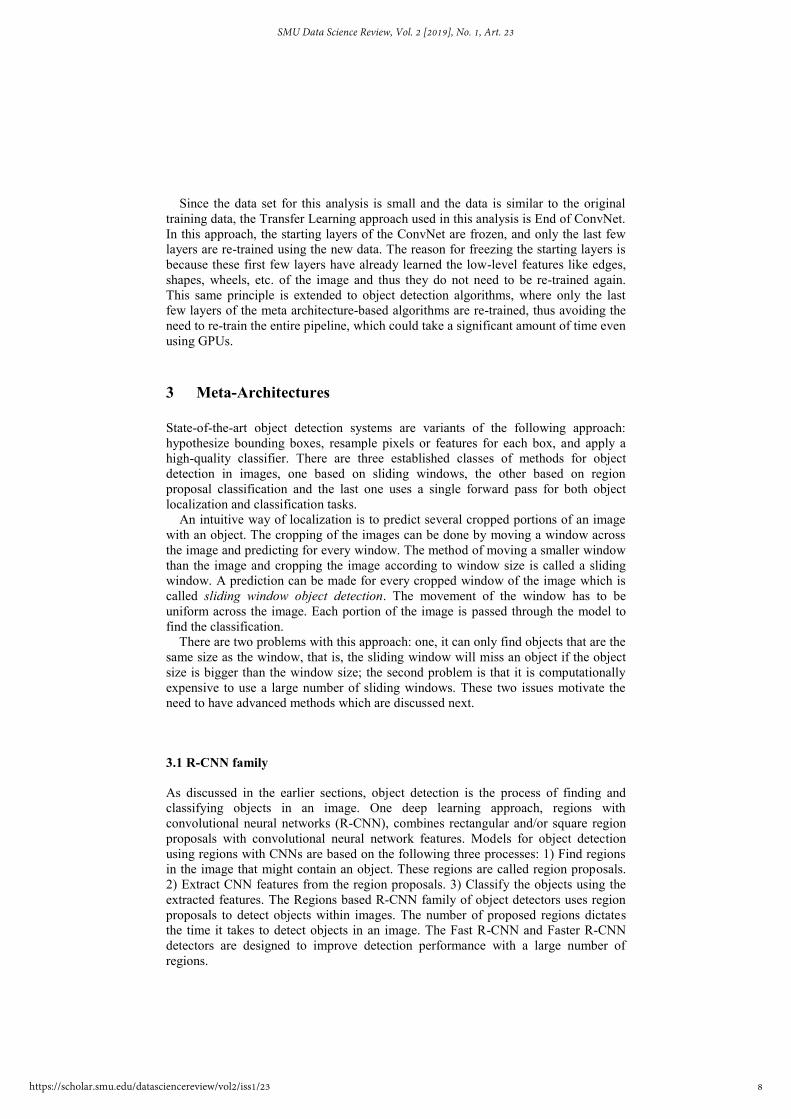
Since the data set for this analysis is small and the data is similar to the original

training data, the Transfer Learning approach used in this analysis is End of ConvNet.

In this approach, the starting layers of the ConvNet are frozen, and only the last few

layers are re-trained using the new data. The reason for freezing the starting layers is

because these first few layers have already learned the low-level features like edges,

shapes, wheels, etc. of the image and thus they do not need to be re-trained again.

This same principle is extended to object detection algorithms, where only the last

few layers of the meta architecture-based algorithms are re-trained, thus avoiding the

need to re-train the entire pipeline, which could take a significant amount of time even

using GPUs.

3 Meta-Architectures

State-of-the-art object detection systems are variants of the following approach:

hypothesize bounding boxes, resample pixels or features for each box, and apply a

high-quality classifier. There are three established classes of methods for object

detection in images, one based on sliding windows, the other based on region

proposal classification and the last one uses a single forward pass for both object

localization and classification tasks.

An intuitive way of localization is to predict several cropped portions of an image

with an object. The cropping of the images can be done by moving a window across

the image and predicting for every window. The method of moving a smaller window

than the image and cropping the image according to window size is called a sliding

window. A prediction can be made for every cropped window of the image which is

called sliding window object detection. The movement of the window has to be

uniform across the image. Each portion of the image is passed through the model to

find the classification.

There are two problems with this approach: one, it can only find objects that are the

same size as the window, that is, the sliding window will miss an object if the object

size is bigger than the window size; the second problem is that it is computationally

expensive to use a large number of sliding windows. These two issues motivate the

need to have advanced methods which are discussed next.

3.1 R-CNN family

As discussed in the earlier sections, object detection is the process of finding and

classifying objects in an image. One deep learning approach, regions with

convolutional neural networks (R-CNN), combines rectangular and/or square region

proposals with convolutional neural network features. Models for object detection

using regions with CNNs are based on the following three processes: 1) Find regions

in the image that might contain an object. These regions are called region proposals.

2) Extract CNN features from the region proposals. 3) Classify the objects using the

extracted features. The Regions based R-CNN family of object detectors uses region

proposals to detect objects within images. The number of proposed regions dictates

the time it takes to detect objects in an image. The Fast R-CNN and Faster R-CNN

detectors are designed to improve detection performance with a large number of

regions.

8



Region Proposal Network (RPN) ranks region on boxes, referred to as anchors, and

proposes the ones most likely containing objects. RPN predicts the possibility on an

anchor being background or foreground. The output of an RPN is a bunch of

boxes/proposals that will be examined by a classifier and regressor, to check the

occurrence of objects eventually. The overall loss of the RPN is a combination of the

classification loss and the regression loss.

Non-max suppression method is used at the end of the network to discard a large

number of predicted boxes based on higher Intersection over Union (IoU) threshold

(larger overlapping) and with the highest prediction of the probability of an object

existence – and merge highly overlapping bounding boxes.

After RPN, the network yields proposed regions with different sizes, means

different sized CNN feature maps. To simplify the differently sized feature maps into

the same size, Regions of Interest (ROI) Pooling is used, by reducing the regression

output to a fixed size output regardless of input size.

There are three variants of an R-CNN. Each variant attempt to optimize, speed up

or enhance the results of one or more of these processes.

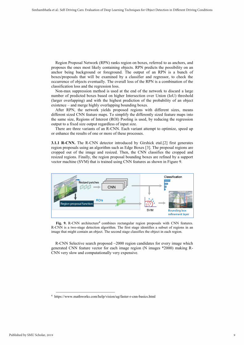
3.1.1 R-CNN. The R-CNN detector introduced by Girshick etal.[2] first generates

region proposals using an algorithm such as Edge Boxes [3]. The proposal regions are

cropped out of the image and resized. Then, the CNN classifies the cropped and

resized regions. Finally, the region proposal bounding boxes are refined by a support

vector machine (SVM) that is trained using CNN features as shown in Figure 9.

Fig. 9. R-CNN architecture4 combines rectangular region proposals with CNN features.

R-CNN is a two-stage detection algorithm. The first stage identifies a subset of regions in an

image that might contain an object. The second stage classifies the object in each region.

R-CNN Selective search proposed ~2000 region candidates for every image which

generated CNN feature vector for each image region (N images *2000) making R-

CNN very slow and computationally very expensive.

4 https://www.mathworks.com/help/vision/ug/faster-r-cnn-basics.html

9



3.1.2 Fast R-CNN. As in the R-CNN detector [2], the Fast R-CNN [4] detector also

uses an algorithm like Edge Boxes to generate region proposals. Unlike the R-CNN

detector, which crops and resizes region proposals, the Fast R-CNN detector

processes the entire image. Whereas an R-CNN detector must classify each region,

Fast R-CNN pools CNN features corresponding to each region proposal as shown in

Figure 10. Fast R-CNN is more efficient than R-CNN, because, in the Fast R-CNN

detector, the computations for overlapping regions are shared.

Fig. 10. Fast R-CNN architecture5: Unlike the R-CNN detector, which crops and resizes region

proposals, the Fast R-CNN detector processes the entire image.

Fast R-CNN is much faster in both training and testing time than the base R-CNN.

However, the improvement is not dramatic because the region proposals are generated

separately by another model and that is very expensive.

3.1.3 Faster R-CNN. In the Faster R-CNN detector, instead of using an external

algorithm like Edge Boxes, Faster R-CNN adds a region proposal network (RPN) to

generate region proposals directly in the network (Figure 11). Generating region

proposals in the network is faster and better tuned to the input data.

Fig. 11 Faster R-CNN5: Instead of using an external algorithm like Edge Boxes, Faster R-CNN

adds a region proposal network (RPN) to generate region proposals directly in the network.

In this paper, pre-trained models using Faster R-CNN are used to leverage optimal

and accurate regional proposal generation. This aids to improve regional proposal

quality of the networks and overall object detection accuracy in an image

5 https://www.mathworks.com/help/vision/ug/faster-r-cnn-basics.html

10



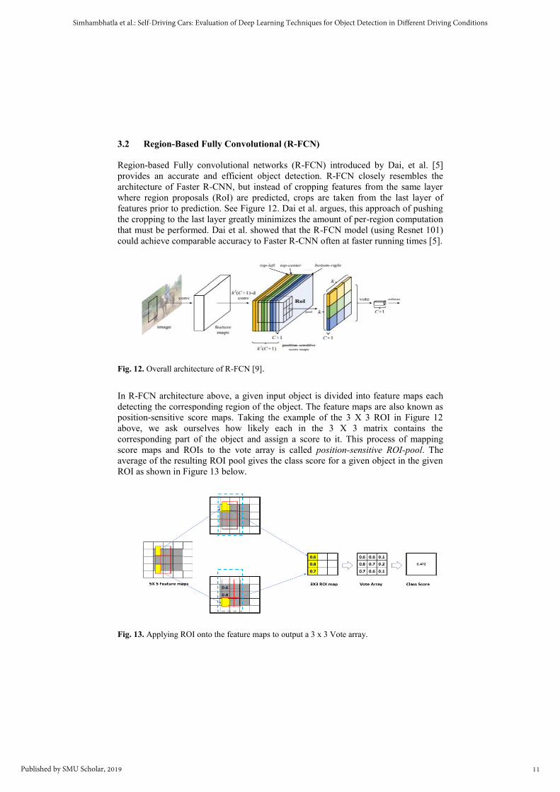
3.2 Region-Based Fully Convolutional (R-FCN)

Region-based Fully convolutional networks (R-FCN) introduced by Dai, et al. [5]

provides an accurate and efficient object detection. R-FCN closely resembles the

architecture of Faster R-CNN, but instead of cropping features from the same layer

where region proposals (RoI) are predicted, crops are taken from the last layer of

features prior to prediction. See Figure 12. Dai et al. argues, this approach of pushing

the cropping to the last layer greatly minimizes the amount of per-region computation

that must be performed. Dai et al. showed that the R-FCN model (using Resnet 101)

could achieve comparable accuracy to Faster R-CNN often at faster running times [5].

Fig. 12. Overall architecture of R-FCN [9].

In R-FCN architecture above, a given input object is divided into feature maps each

detecting the corresponding region of the object. The feature maps are also known as

position-sensitive score maps. Taking the example of the 3 X 3 ROI in Figure 12

above, we ask ourselves how likely each in the 3 X 3 matrix contains the

corresponding part of the object and assign a score to it. This process of mapping

score maps and ROIs to the vote array is called position-sensitive ROI-pool. The

average of the resulting ROI pool gives the class score for a given object in the given

ROI as shown in Figure 13 below.

Fig. 13. Applying ROI onto the feature maps to output a 3 x 3 Vote array.

11



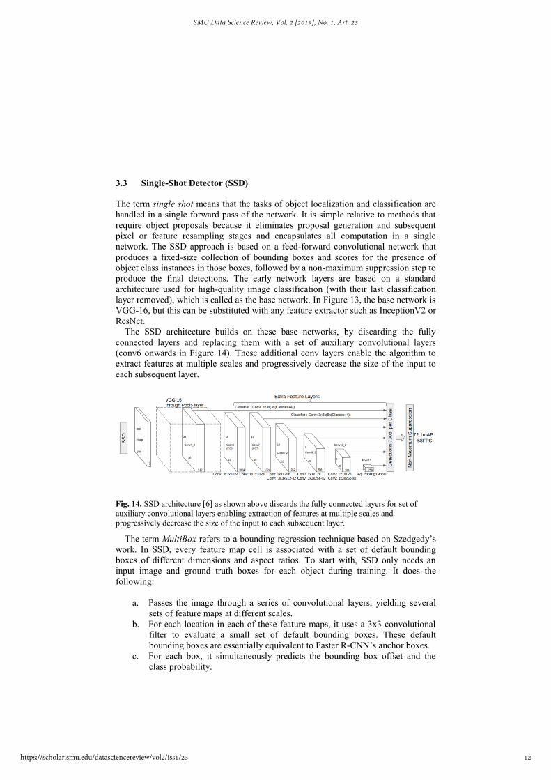
3.3 Single-Shot Detector (SSD)

The term single shot means that the tasks of object localization and classification are

handled in a single forward pass of the network. It is simple relative to methods that

require object proposals because it eliminates proposal generation and subsequent

pixel or feature resampling stages and encapsulates all computation in a single

network. The SSD approach is based on a feed-forward convolutional network that

produces a fixed-size collection of bounding boxes and scores for the presence of

object class instances in those boxes, followed by a non-maximum suppression step to

produce the final detections. The early network layers are based on a standard

architecture used for high-quality image classification (with their last classification

layer removed), which is called as the base network. In Figure 13, the base network is

VGG-16, but this can be substituted with any feature extractor such as InceptionV2 or

ResNet.

The SSD architecture builds on these base networks, by discarding the fully

connected layers and replacing them with a set of auxiliary convolutional layers

(conv6 onwards in Figure 14). These additional conv layers enable the algorithm to

extract features at multiple scales and progressively decrease the size of the input to

each subsequent layer.

Fig. 14. SSD architecture [6] as shown above discards the fully connected layers for set of

auxiliary convolutional layers enabling extraction of features at multiple scales and

progressively decrease the size of the input to each subsequent layer.

The term MultiBox refers to a bounding regression technique based on Szedgedy’s

work. In SSD, every feature map cell is associated with a set of default bounding

boxes of different dimensions and aspect ratios. To start with, SSD only needs an

input image and ground truth boxes for each object during training. It does the

following:

a. Passes the image through a series of convolutional layers, yielding several

sets of feature maps at different scales.

b. For each location in each of these feature maps, it uses a 3x3 convolutional

filter to evaluate a small set of default bounding boxes. These default

bounding boxes are essentially equivalent to Faster R-CNN’s anchor boxes.

c. For each box, it simultaneously predicts the bounding box offset and the

class probability.

12



d. During training, it matches the ground truth box with these predicted boxes

based on Intersection over Union (IoU). The best-predicted box will be

labeled a positive, along with all the other boxes that have an IoU with the

truth > 0.5.

Since SSD does not have a region proposal network, which would have ensured

that everything we tried to classify had some minimum probability of being an

“object”, instead we end up with a greater number of bounding boxes with many of

them having negative examples. To fix this imbalance, SSD does two things. First, it

uses non-maximum suppression (NMS) to group together highly-overlapping boxes

into a single box. For instance, in Figure 15, if four boxes contain the same dog, NMS

would keep the one with the highest confidence and discard the rest. Secondly, the

model uses a technique called hard negative mining to balance classes during training.

In this technique, only a subset of the negative examples with the highest training loss

are used at each iteration of training. SSD keeps a 3:1 ratio of negatives to positives.

The varying-size feature maps which are generated due to the extra feature layers

help SSD tackle the scale problem. In smaller feature maps (e.g., 4x4), each cell

covers a larger region of the image, enabling them to detect larger objects. Region

proposal and classification are performed simultaneously: given p object classes, each

bounding box is associated with a (4+p)-dimensional vector that outputs 4 box offset

coordinates and p class probabilities. In the last step, softmax is again used to classify

the object.

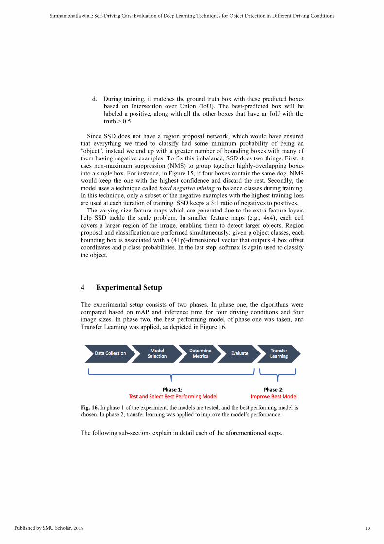
4 Experimental Setup

The experimental setup consists of two phases. In phase one, the algorithms were

compared based on mAP and inference time for four driving conditions and four

image sizes. In phase two, the best performing model of phase one was taken, and

Transfer Learning was applied, as depicted in Figure 16.

Fig. 16. In phase 1 of the experiment, the models are tested, and the best performing model is

chosen. In phase 2, transfer learning was applied to improve the model’s performance.

The following sub-sections explain in detail each of the aforementioned steps.

13



4.1 Data Collection

Most object detection models use Convolutional Neural Network (CNN) methods to

train images and detect objects by identifying a region of interest within that image

and determine the class of the object present within that region. Testing the pre-

trained object detection models requires test images that contain reasonable clarity

and visibility of the classes being identified – which the probability of detection

depends.

4.1.1 Data sources. Various data sources were examined, including Google, and large

University of California at Berkeley Deep Drive data sets [7]. We acquired sample

data sets from Berkeley’s video database and extracted images from videos we

recorded while at traffic stops and parking lots at our neighborhoods. Samples taken

covered different driving conditions: daytime, rainy, snowy and night.

4.1.2 Annotations using labelImg. To measure the performance of the object

detection algorithms, a reference to the location of objects in the images is needed.

COCO annotation format was followed to label target object classes using bounding

boxes. These reference bounding boxes indicating the true location of objects in the

images are referred to as GroundTruth. Comparing this GroundTruth bounding boxes

to the predicted bounding boxes that are generated by the algorithms is what gives us

the accuracy of the Object detection algorithm summarized by the mAP score.

A Windows Operating System open source software, LabelImg [11] was used to

annotate the images. The tool allows the use of text file with predefined classes which

made it easy to maintain the same class IDs as those in COCO dataset.

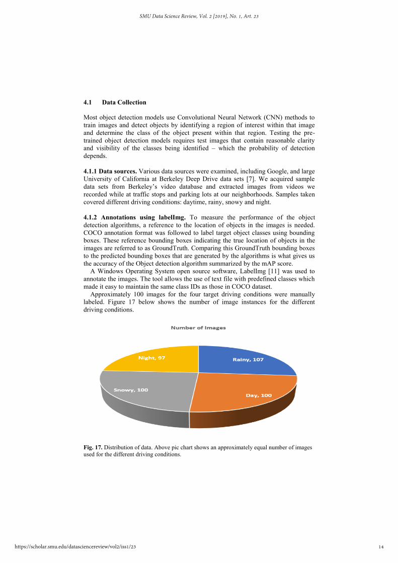
Approximately 100 images for the four target driving conditions were manually

labeled. Figure 17 below shows the number of image instances for the different

driving conditions.

Fig. 17. Distribution of data. Above pic chart shows an approximately equal number of images

used for the different driving conditions.

14



4.2 Model Selection

TensorFlow’s object detection model zoo [8] provides several models that are pre-

trained on the COCO dataset and made available for out-of-the-box inference. Since

all these models were trained on the COCO dataset, they can be used for detecting the

objects that are available in the COCO dataset such as humans and cars.

Three models: faster_rcnn_inception_v2_coco, ssd_inception_v2_coco, and

rfcn_resnet101_coco, were chosen from the model zoo, that represent the three meta-

architectures that are being compared in this research. The model names identify the

meta-architecture, the feature extractor, and the training data used. For instance, the

faster_rcnn_inception_v2_coco model uses faster R-CNN as the meta-architecture,

inceptionv2 as its feature extractor that has been trained on COCO dataset.

In addition to providing out-of-the-box inference, TensorFlow’s object detection

API also makes it possible to apply transfer learning to these models using a

customizable config file to either extend or fine-tune these models.

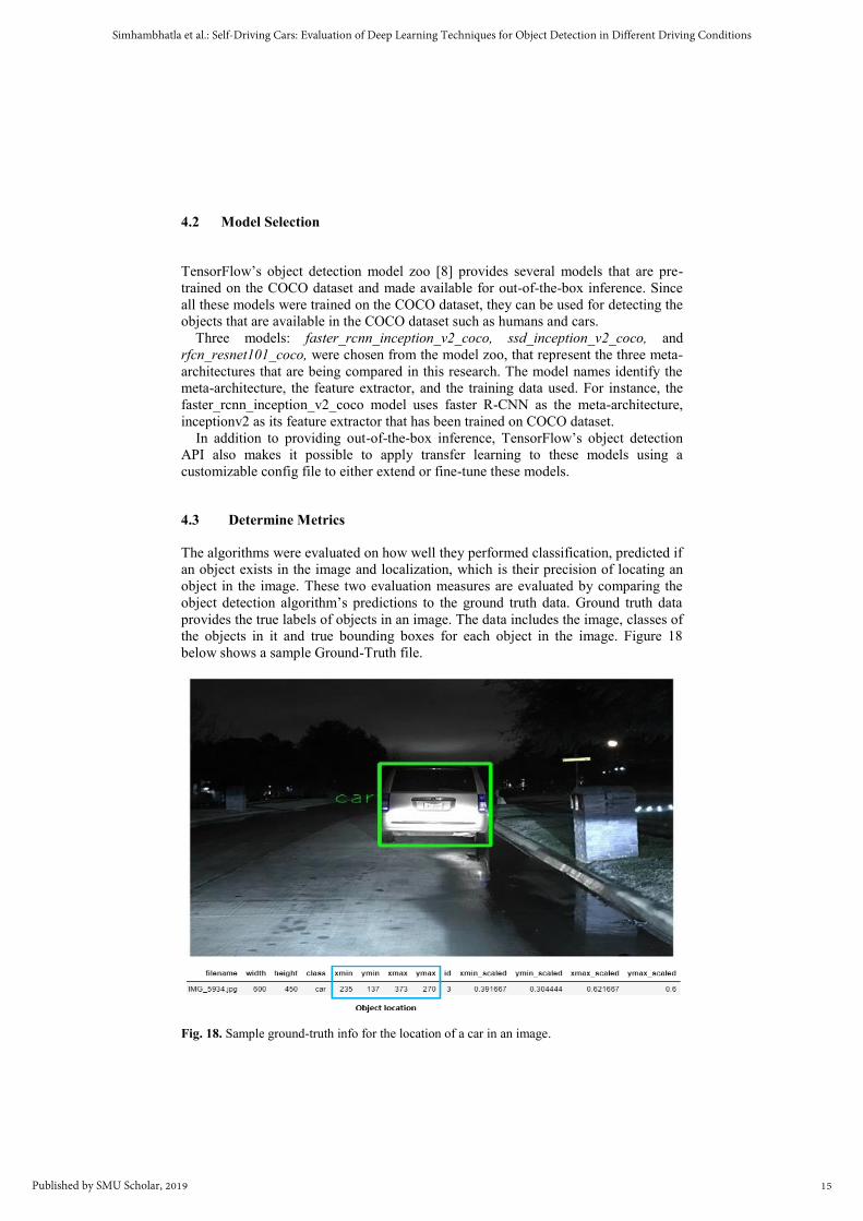
4.3 Determine Metrics

The algorithms were evaluated on how well they performed classification, predicted if

an object exists in the image and localization, which is their precision of locating an

object in the image. These two evaluation measures are evaluated by comparing the

object detection algorithm’s predictions to the ground truth data. Ground truth data

provides the true labels of objects in an image. The data includes the image, classes of

the objects in it and true bounding boxes for each object in the image. Figure 18

below shows a sample Ground-Truth file.

Fig. 18. Sample ground-truth info for the location of a car in an image.

15



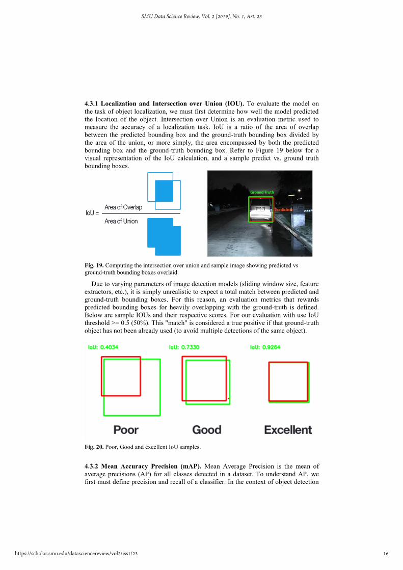
4.3.1 Localization and Intersection over Union (IOU). To evaluate the model on

the task of object localization, we must first determine how well the model predicted

the location of the object. Intersection over Union is an evaluation metric used to

measure the accuracy of a localization task. IoU is a ratio of the area of overlap

between the predicted bounding box and the ground-truth bounding box divided by

the area of the union, or more simply, the area encompassed by both the predicted

bounding box and the ground-truth bounding box. Refer to Figure 19 below for a

visual representation of the IoU calculation, and a sample predict vs. ground truth

bounding boxes.

Fig. 19. Computing the intersection over union and sample image showing predicted vs

ground-truth bounding boxes overlaid.

Due to varying parameters of image detection models (sliding window size, feature

extractors, etc.), it is simply unrealistic to expect a total match between predicted and

ground-truth bounding boxes. For this reason, an evaluation metrics that rewards

predicted bounding boxes for heavily overlapping with the ground-truth is defined.

Below are sample IOUs and their respective scores. For our evaluation with use IoU

threshold >= 0.5 (50%). This "match" is considered a true positive if that ground-truth

object has not been already used (to avoid multiple detections of the same object).

Fig. 20. Poor, Good and excellent IoU samples.

4.3.2 Mean Accuracy Precision (mAP). Mean Average Precision is the mean of

average precisions (AP) for all classes detected in a dataset. To understand AP, we

first must define precision and recall of a classifier. In the context of object detection

16



algorithms, precision measures the “false positive rate” or the ratio of true object

detections to the total number of objects that the classifier predicted. If you have a

high precision rate, there is a high likelihood that whatever the classifier predicts as a

positive detection is, in fact, a correct prediction. On the other hand, recall measures

the “false negative rate” or the ratio of true object detections to the total number of

objects in the data set. A high recall score means the model will positively detect all

objects that are in the dataset. It is worth noting that, these two metrics are inversely

related, and they are dependent on the model’s performance and the threshold set for

the model score. Figure 21 below shows formulas for calculating precision and recall.

Fig. 21. Precision and Recall formulas

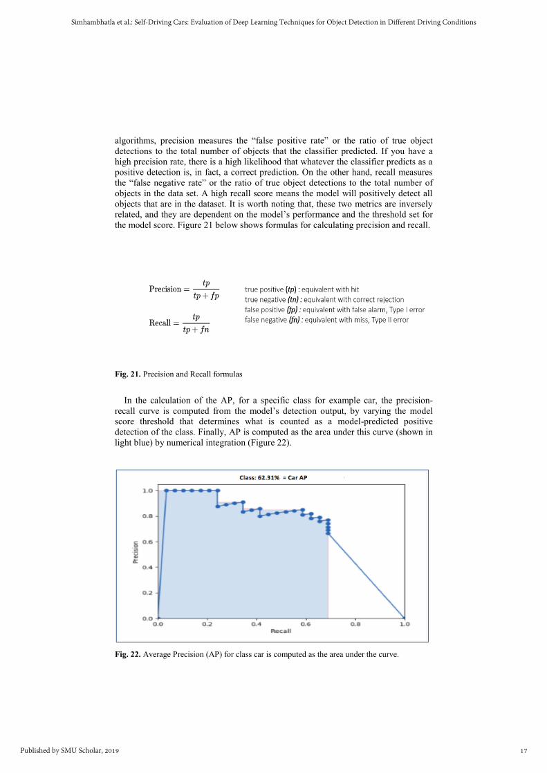
In the calculation of the AP, for a specific class for example car, the precision-

recall curve is computed from the model’s detection output, by varying the model

score threshold that determines what is counted as a model-predicted positive

detection of the class. Finally, AP is computed as the area under this curve (shown in

light blue) by numerical integration (Figure 22).

Fig. 22. Average Precision (AP) for class car is computed as the area under the curve.

17



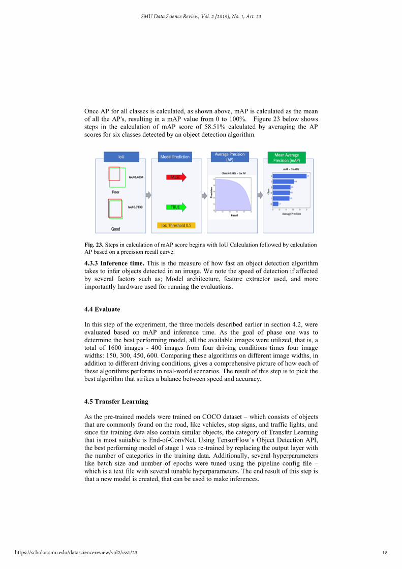
Once AP for all classes is calculated, as shown above, mAP is calculated as the mean

of all the AP's, resulting in a mAP value from 0 to 100%. Figure 23 below shows

steps in the calculation of mAP score of 58.51% calculated by averaging the AP

scores for six classes detected by an object detection algorithm.

Fig. 23. Steps in calculation of mAP score begins with IoU Calculation followed by calculation

AP based on a precision recall curve.

4.3.3 Inference time. This is the measure of how fast an object detection algorithm

takes to infer objects detected in an image. We note the speed of detection if affected

by several factors such as; Model architecture, feature extractor used, and more

importantly hardware used for running the evaluations.

4.4 Evaluate

In this step of the experiment, the three models described earlier in section 4.2, were

evaluated based on mAP and inference time. As the goal of phase one was to

determine the best performing model, all the available images were utilized, that is, a

total of 1600 images - 400 images from four driving conditions times four image

widths: 150, 300, 450, 600. Comparing these algorithms on different image widths, in

addition to different driving conditions, gives a comprehensive picture of how each of

these algorithms performs in real-world scenarios. The result of this step is to pick the

best algorithm that strikes a balance between speed and accuracy.

4.5 Transfer Learning

As the pre-trained models were trained on COCO dataset – which consists of objects

that are commonly found on the road, like vehicles, stop signs, and traffic lights, and

since the training data also contain similar objects, the category of Transfer Learning

that is most suitable is End-of-ConvNet. Using TensorFlow’s Object Detection API,

the best performing model of stage 1 was re-trained by replacing the output layer with

the number of categories in the training data. Additionally, several hyperparameters

like batch size and number of epochs were tuned using the pipeline config file –

which is a text file with several tunable hyperparameters. The end result of this step is

that a new model is created, that can be used to make inferences.

18



5 Environment

5.1 Hardware environment

When working with large amounts of data and complex network architectures, GPUs

can significantly speed the processing time. These models were evaluated and trained

on Ubuntu 16.04 with GPU: GeForce GTX 1060 with 16GB memory. TensorFlow

with CUDA toolkit 9.2 and cuDNNv7.0 was used to train the models during Transfer

Learning phase.

5.2 Tools

Google released pre-trained models with various algorithms trained on the COCO

dataset for public use [8]. The API is built on top of TensorFlow and intended for

constructing, training, and deploying object detection models. The APIs support both

object detection and localization tasks. The availability of pre-trained models enables

the fine-tuning of new data and hence making the training faster.

6 Results

In phase one of our experiment, the algorithms are evaluated to determine which

works best under different driving conditions. In phase two, Transfer Learning is

applied to the model selected from phase one. The results are discussed in two phases.

6.1 Phase 1: Determine the best model

6.1.1 Heat Map of mAP scores across algorithms and driving conditions: As

discussed in the evaluation section 4.3.2 above, mean Average Precision (mAP) is the

primary evaluation metric used, and it is the average of the maximum precisions at

different recall values. mAP gives a one number summary measuring the accuracy of

localization and classification for a given object detection algorithm. In Figure 24

below, the mAP heatmap for varying image width on different driving conditions for

the three Meta-Architecture is shown. Considering that the pre-trained models were

trained on COCO dataset image size, 600 X 600 as indicated on the TensorFlow

Model Zoo directory [8], varying the image width is impacts the mAP score achieved

by a given algorithm. mAP score increases as the image width increases from 150 to

600. Region-based architecture i.e., R-FCN and Faster R-CNN outperformed the

SSD. For the limited dataset used, all the algorithms have higher mAP scores for the

snowy condition compared to the rest of the conditions.

19



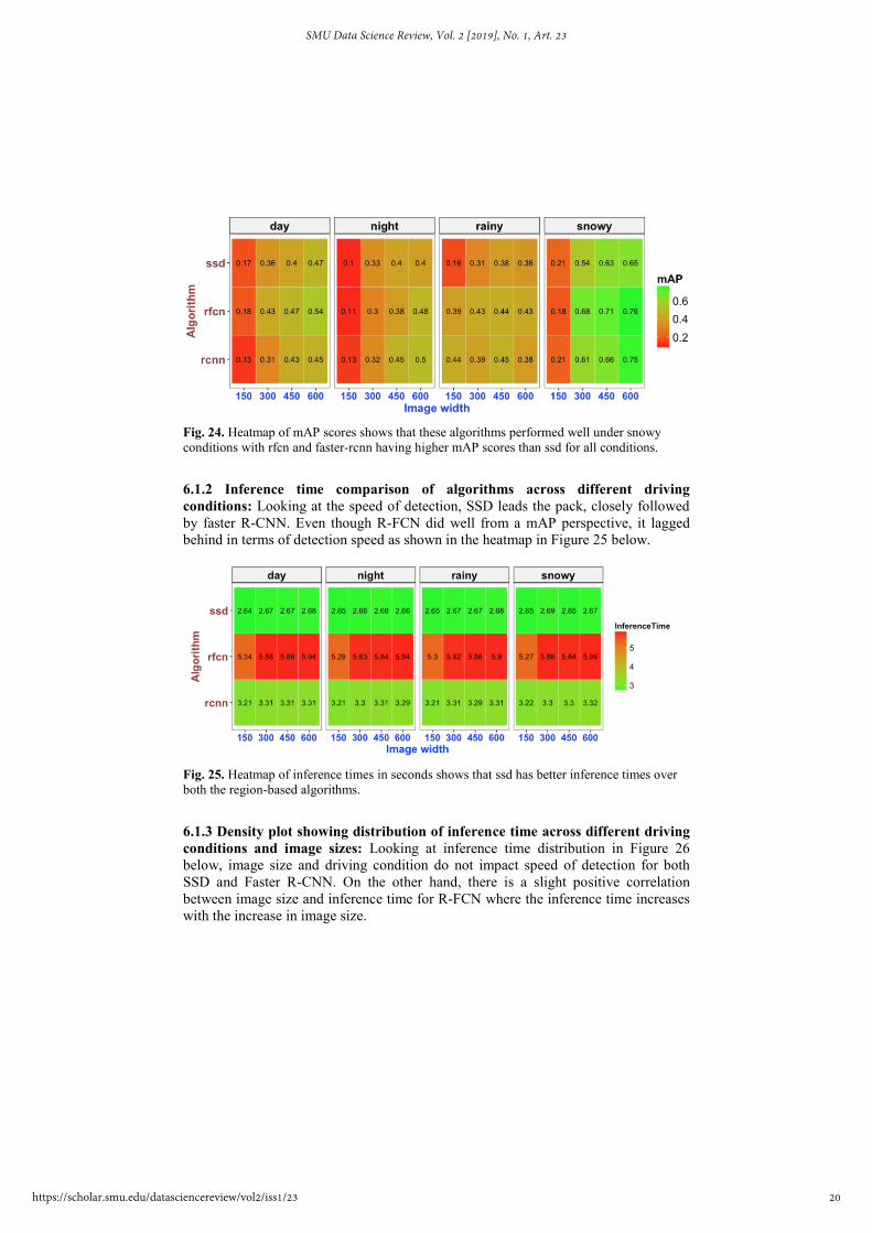
Fig. 24. Heatmap of mAP scores shows that these algorithms performed well under snowy

conditions with rfcn and faster-rcnn having higher mAP scores than ssd for all conditions.

6.1.2 Inference time comparison of algorithms across different driving

conditions: Looking at the speed of detection, SSD leads the pack, closely followed

by faster R-CNN. Even though R-FCN did well from a mAP perspective, it lagged

behind in terms of detection speed as shown in the heatmap in Figure 25 below.

Fig. 25. Heatmap of inference times in seconds shows that ssd has better inference times over

both the region-based algorithms.

6.1.3 Density plot showing distribution of inference time across different driving

conditions and image sizes: Looking at inference time distribution in Figure 26

below, image size and driving condition do not impact speed of detection for both

SSD and Faster R-CNN. On the other hand, there is a slight positive correlation

between image size and inference time for R-FCN where the inference time increases

with the increase in image size.

20



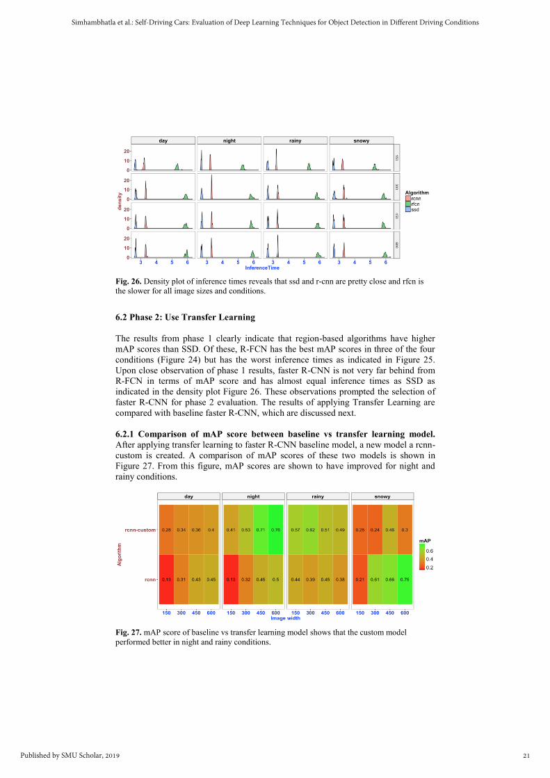
Fig. 26. Density plot of inference times reveals that ssd and r-cnn are pretty close and rfcn is

the slower for all image sizes and conditions.

6.2 Phase 2: Use Transfer Learning

The results from phase 1 clearly indicate that region-based algorithms have higher

mAP scores than SSD. Of these, R-FCN has the best mAP scores in three of the four

conditions (Figure 24) but has the worst inference times as indicated in Figure 25.

Upon close observation of phase 1 results, faster R-CNN is not very far behind from

R-FCN in terms of mAP score and has almost equal inference times as SSD as

indicated in the density plot Figure 26. These observations prompted the selection of

faster R-CNN for phase 2 evaluation. The results of applying Transfer Learning are

compared with baseline faster R-CNN, which are discussed next.

6.2.1 Comparison of mAP score between baseline vs transfer learning model.

After applying transfer learning to faster R-CNN baseline model, a new model a rcnn-

custom is created. A comparison of mAP scores of these two models is shown in

Figure 27. From this figure, mAP scores are shown to have improved for night and

rainy conditions.

Fig. 27. mAP score of baseline vs transfer learning model shows that the custom model

performed better in night and rainy conditions.

21



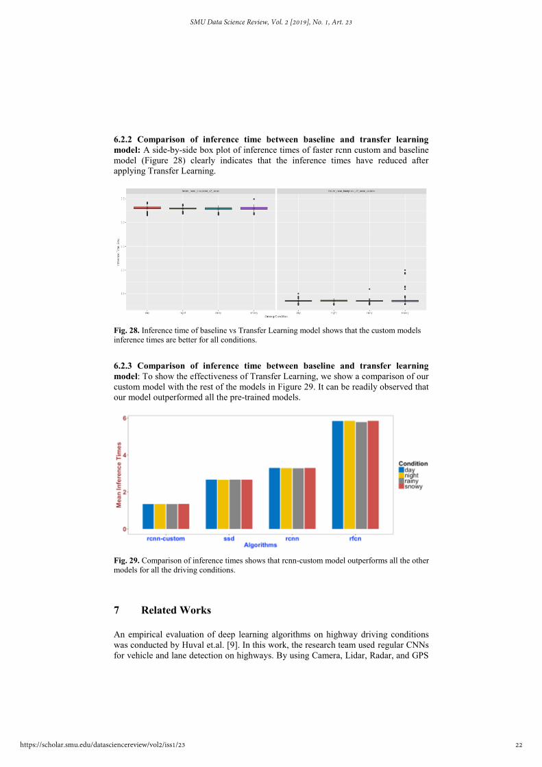
6.2.2 Comparison of inference time between baseline and transfer learning

model: A side-by-side box plot of inference times of faster rcnn custom and baseline

model (Figure 28) clearly indicates that the inference times have reduced after

applying Transfer Learning.

Fig. 28. Inference time of baseline vs Transfer Learning model shows that the custom models

inference times are better for all conditions.

6.2.3 Comparison of inference time between baseline and transfer learning

model: To show the effectiveness of Transfer Learning, we show a comparison of our

custom model with the rest of the models in Figure 29. It can be readily observed that

our model outperformed all the pre-trained models.

Fig. 29. Comparison of inference times shows that rcnn-custom model outperforms all the other

models for all the driving conditions.

7 Related Works

An empirical evaluation of deep learning algorithms on highway driving conditions

was conducted by Huval et.al. [9]. In this work, the research team used regular CNNs

for vehicle and lane detection on highways. By using Camera, Lidar, Radar, and GPS

22



they built a highway dataset consisting of 17 thousand image frames with vehicle

bounding boxes and over 616 thousand image frames with lane annotations. Using

this dataset, they trained a CNN and showed that regular CNNs are capable of

detecting vehicles and cars in a single forward pass. Their results show that CNN

algorithms are capable of good performance in highway lane and vehicle detection,

however their work omitted temporal information which is an important component in

lane and vehicle detection systems.

Many object detection algorithms have been developed in the recent years which

are based on Convolutional Neural Networks. While each algorithm has individually

presented its speed and accuracy metrics, what is lacking is a comprehensive

comparison of these algorithms. Dai et al, presented a region-based fully

convolutional network (R-FCN) for object detection and reported that they achieved

an accuracy close to Faster R-CNN but with better training time [10]. Liu et al.

introduced SSD [6], a single-shot detector for multiple categories that is faster than

the previous state-of-the-art for single shot detectors (YOLO), and significantly more

accurate, in fact, as accurate as slower techniques that perform explicit region

proposals and pooling (including Faster R-CNN). Finding a way to do an apples-to-

apples comparison of these algorithms is the biggest challenge. For instance, some

algorithms use different base feature extractors like VGG or Residual Networks,

while some others work well with certain image resolutions and yet some others have

been specifically trained on certain hardware and software platforms. Huang, et al.

attempted to address this problem by using a unified implementation of Faster R-

CNN, R-FCN and SSD systems, which they call as "meta-architectures" [12].

The idea behind using a unified approach is that it is impractical to compare every

recently proposed detection system. By grouping algorithms based on common set of

architectures, it is possible to compare many algorithms that share similar

characteristics. In particular, the group of researchers have created implementations of

the Faster R-CNN, R-FCN and SSD meta-architectures, which at a high level consist

of a single convolutional network, trained with a mixed regression and classification

objective, and use sliding window style predictions. The results show that using fewer

proposals for Faster R-CNN can speed it up significantly without a big loss in

accuracy, making it competitive with its faster cousins, SSD and R-FCN. They also

showed that SSDs performance is less sensitive to the quality of the feature extractor

than Faster R-CNN and R-FCN.

The speed and accuracy trade-off– the gains in accuracy are only possible by

sacrificing speed and vice-versa, is a ubiquitous problem in self-driving cars. The

decision to choose one architecture over other boils down to finding the sweet spot

between accuracy/speed trade-off curve. An empirical evaluation of the performance

of these architectures/algorithms for solving object detection problems in the context

of self-driving cars under varying driving conditions has not been attempted.

8 Ethics

We have acquired our test data from Berkley object detection data repository [7] and

videos recorded around our neighborhoods. We have used a python script to extract

some of images used for research.

We believe we have acted responsibly and professionally while handling the test

data in our hand, with the intension of evaluating and improving existing object

23



detection algorithms in the context of Self Driving cars, expected to support the

public good. In that way, we completely adhere to “The ACM Code of Ethics and

Professional Conduct [13] guidelines.

We adhere to General Ethical Principles as our work would definitely fit into one

of a kind research specific to evaluating top quality object detection models

potentially used in the race of finding best solutions for object detection technology in

the inevitable Self Driving Car future. Our research is honest and trustworthy, did not

pose harm to any stakeholder as this is not implemented or not in the process of

capturing data, expected to contribute to society and to human well-being if this

research can be used for further studies. The research required adaption from lot of

great work already done in this area, and leveraged already existing tools, code,

journals as cited in the paper to respect others work, innovations and creativity. The

test data collected and used for testing is not expected to be published on social sites

or used for any commercial purposes to respect the privacy and honor confidentiality

of the subjects in the images.

We strongly acted upon our Professional Responsibilities to strive to achieve high

quality in both the processes and products of professional work. We have leveraged

existing object detection models available from COCO object model zoo [8], open

source tools such as LabelImg [11] for creating ground truth labels and annotation.

We take pride having demonstrated our Professional Leadership Principles by

developing an idea that can further create more opportunities for members of the Data

Scientist community and professional working on similar projects in near future. A

fail-proof all-weather solution is extremely needed for the success of Self Driving Car

to operate safely and socially acceptance environment.

Finally, the project is completely technical in nature and applied various deep

learning techniques. The progress should not have been possible without amazing and

extensive work done by many researchers that we leveraged as explained in the earlier

sections. By citing the references in our paper, we uphold, promote and respect the

principles of Compliance with the Code.

9 Conclusion

Based on the study, we conclude that no single algorithm works best for all

conditions. However, retraining and optimizing with domain-specific data using

Transfer Learning is likely to improve performance in similar conditions.

In this research, we have evaluated the performance of 3 object detection

architectures based on the 2 metrics - mAP score and inference time. Our results show

that region-based algorithms such as Faster R-CNN and R-FCN tend to have a high

accuracy and SSD based algorithms have faster inference times. As our dataset

comprised of images taken under four different driving conditions, we were able to

evaluate the performance of each of these algorithms under different driving

conditions. Our results show that these algorithms tend to perform well under snowy

conditions. We also proved that we can take a generic pre-trained model and apply

transfer learning to improve the inference times by about three seconds per image.

Transfer learning also proved to be effective in improving the mAP scores even with

a small training dataset of 240 images (60 images per condition) for three of the four

conditions.

24



10 Future Work

The research enables much more opportunities to improve further. The number of test

images can be increased substantially and tested with streaming videos to perform

more practical real-world applications of self-driving cars and other autonomous

vehicles or devices. The research can be performed with models from object detection

model zoo and with newer approaches to test similar comparisons under varying

weather conditions. The research can be extended to test the models in real-time self-

driving car implementation by integrating with sensor data. The performance of mAP

scores and inference time can be improved by tuning other hyper-parameters and

additional layers in the Transfer Learning step – using high-performance GPU

systems.

References

1. Hubel, H. D. and Wiesel, T. N. "Receptive Fields of Single neurons in the Cat’s Striate

Cortex." Journal of Physiology. Vol 148, pp. 574-591, 1959.

2. R. Girshick, J. Donahue, T. Darrell, and J. Malik. Rich feature hierarchies for accurate

object detection and semantic segmentation. In Proceedings of the IEEE conference on

computer vision and pattern recognition, pages 580–587, 2014. 2, 5

3. Patterson, Josh, and Adam Gibson. “Deep Learning: A Practitioners Approach”.

Sebastopol, CA: OReilly, 2017. Print.

4. Girshick, ROSS. “Fast R-CNN.” [Astro-Ph/0005112] A Determination of the Hubble

Constant from Cepheid Distances and a Model of the Local Peculiar Velocity Field,

American Physical Society, 27 Sept. 2015, arxiv.org/abs/1504.08083.

5. Dai, et al. “R-FCN: Object Detection via Region-Based Fully Convolutional Networks.”

[Astro-Ph/0005112] A Determination of the Hubble Constant from Cepheid Distances and

a Model of the Local Peculiar Velocity Field, American Physical Society, 21 June 2016,

arxiv.org/abs/1605.06409.

6. Liu, Wei, et al. “SSD: Single Shot Multi-Box Detector.” [Astro-Ph/0005112] A

Determination of the Hubble Constant from Cepheid Distances and a Model of the Local

Peculiar Velocity Field, American Physical Society, 29 Dec. 2016,


7. “Berkeley DeepDrive.” Berkeley DeepDrive, bdd-data.berkeley.edu/.

8. TensorFlow Object Detection Model zoo:

https://github.com/tensorflow/models/blob/master/research/object_detection/g3doc/detecti

on_model_zoo.md

9. Huval, B., Wang, T., Tandon, S., et al. (2015). An empirical evaluation of deep learning

on highway driving. arXiv preprint arXiv:1504.01716

10. S. Ren, K. He, R. Girshick, and J. Sun. Faster R-CNN: Towards real-time object detection

with region proposal networks. In NIPS, 2015

11. LabelImg tool Github repository: https://github.com/tzutalin/labelImg

12. Huang, et al. “Speed/Accuracy Trade-Offs for Modern Convolutional Object Detectors.”


a Model of the Local Peculiar Velocity Field, 25 Apr. 2017, arxiv.org/abs/1611.10012.

13. The ACM Code of Ethics and Professional Conduct: https://www.acm.org/code-of-ethics

14. Redmon, Joseph, et al. “You Only Look Once: Unified, Real-Time Object Detection.”


25



https://github.com/tensorflow/models/blob/master/research/object_detection/g3doc/detection_model_zoo.md

https://github.com/tensorflow/models/blob/master/research/object_detection/g3doc/detection_model_zoo.md

https://github.com/tzutalin/labelImg

https://www.acm.org/code-of-ethics

a Model of the Local Peculiar Velocity Field, American Physical Society, 9 May 2016,


15. Ren, Shaoqing, et al. “Faster R-CNN: Towards Real-Time Object Detection with Region

Proposal Networks.” [Astro-Ph/0005112] A Determination of the Hubble Constant from

Cepheid Distances and a Model of the Local Peculiar Velocity Field, American Physical

Society, 6 Jan. 2016, arxiv.org/abs/1506.01497.

16. Knight, Will. “The Future of Self-Driving Cars.” MIT Technology Review, MIT

Technology Review, 8 July 2016, www.technologyreview.com/s/520431/driverless-cars-

are-further-away-than-you-think/.

17. Redmon, Joseph. “YOLO: Real-Time Object Detection.” YOLO: Real-Time Object

Detection, pjreddie.com/darknet/yolo/

18. Huang, Jonathan, and Vivek Rathod. “Supercharge Your Computer Vision Models with

the TensorFlow Object Detection API.” Google AI Blog, Google AI, 15 June 2017,

ai.googleblog.com/2017/06/supercharge-your-computer-vision-models.html.

19. Ouaknine, Arthur. “Review of Deep Learning Algorithms for Object Detection.” Medium,

Medium, 5 Feb. 2018, medium.com/comet-app/review-of-deep-learning-algorithms-for-

object-detection-c1f3d437b852.

20. R. Girshick, J. Donahue, T. Darrell, and J. Malik. Rich feature hierarchies for accurate

object detection and semantic segmentation. In Proceedings of the IEEE conference on

computer vision and pattern recognition, pages 580–587, 2014. 2, 5

21. R. Girshick. Fast r-cnn. In Proceedings of the IEEE International Conference on Computer

Vision, pages 1440–1448, 2015. 2, 3, 5

22. Zitnick, C. Lawrence, and P. Dollar. "Edge boxes: Locating object proposals from

edges." Computer Vision-ECCV. Springer International Publishing. Pages 391-4050.

2014.

Appendix:

Project Code Location

The Project code is stored in public GitHub repository, which contain code, data and

documents supporting the research work available at https://github.com/kevin-

okiah/CAPSTONE for reference and further enhancements.

26



http://www.technologyreview.com/s/520431/driverless-cars-are-further-away-than-you-think/

http://www.technologyreview.com/s/520431/driverless-cars-are-further-away-than-you-think/

https://github.com/kevin-okiah/CAPSTONE

https://github.com/kevin-okiah/CAPSTONE

Documents

Self-Driving Cars: Evaluation of Deep Learning Techniques