Self-consistent Global Transport of Metallic Ions with WACCM-XJianfei Wu1,2,3, Wuhu Feng4,5, Han-Li Liu6, Xianghui Xue1,2,3,7, Daniel R. Marsh4,6, and John M.C. Plane4

1CAS Key Laboratory of Geospace Environment, School of Earth and Space Sciences, University of Science and Technologyof China, Hefei, China2CAS Center for Excellence in Comparative Planetology, China3Mengcheng National Geophysical Observatory, School of Earth and Space Sciences, University of Science and Technologyof China, Hefei, China4School of Chemistry, University of Leeds, Leeds, UK5National Center for Atmospheric Science, University of Leeds, Leeds, UK6National Center for Atmospheric Research, Boulder, Colorado, USA7Hefei National Laboratory for the Physical Sciences at the Microscale, University of Science and Technology of China,Hefei, China

Correspondence: Xianghui Xue (xuexh@ustc.edu.cn) and John M. C. Plane (J.M.C.Plane@leeds.ac.uk)

Abstract. The NCAR Whole Atmosphere Community Climate Model with thermosphere and ionosphere eXtension (WACCM-

X) v2.1 has been extended to include the neutral and ion-molecule chemistry and dynamics of three metals (Mg, Na, and Fe),

which are injected into the upper mesosphere/lower thermosphere by meteoric ablation. Here we focus on the self-consistent

electrodynamical transport of metallic ions in both the E and F regions. The model with full ion transport significantly improves

the simulation of global distribution and seasonal variations of Mg+, although the peak density is slightly lower (about 35%5

lower in peak density) compared with the SCIAMACHY measurements. Near the magnetic equator, the diurnal variation in

upward and downward transport of Mg+ is generally consistent with the “ionosphere fountain effect”. The thermospheric dis-

tribution of Fe is shown to be closely coupled to the transport of Fe+. The effect of ion mass on ion transport is also examined:

the lighter ions (Mg+ and Na+) are transported above 150 km more easily than the heavy Fe+. We also examine the impact of

the transport of major molecular ions, NO+ and O+2 , on the distribution of metallic ions.10

1 Introduction

The presence of layers of meteor-ablated metal atoms between 80 and 105 km has been known for decades (Plane et al.,

2015). More recently, there have been a growing number of observations of the thermospheric metal layers up to 200 km. For

example: Chu et al. (2011) reported neutral Fe layer observations up to 155 km at McMurdo, Antarctica (77.8◦S, 166.7◦E);

Gao et al. (2015) found that several observations of Na layers reached up to 170 km, using a large-aperture astronomical15

telescope at Lijiang, China (26.7◦N, 100.0◦E); and Friedman et al. (2013) investigated a descending thermospheric K layer

from altitudes above 155 km at Arecibo, Puerto Rico (18.35◦N, 66.75◦W). These high altitude thermospheric neutral metal

layers are challenging to explain, since ablation occurs predominantly below these altitudes, which raises interesting questions

regarding their formation mechanisms. Neutral metal atoms and their corresponding atomic ions are tightly coupled through

1

ionization (via photo-ionization or charge transfer with ambient ions e.g. NO+ and O+2 ), and neutralization (via dielectronic20

recombination with electrons, or dissociative electron recombination if they have formed a molecular ion) (Plane et al., 2015).

Thus, the vertical and horizontal transport of metallic ions is a key process for controlling the behavior of neutral atoms in the

thermosphere (E and F regions). Interestingly, the reported occurrence of thermospheric metal layers appears to show great

geographical variability, underlining the importance of global ion transport. In addition, metallic ions play a central role in the

formation of thin, concentrated layers of ions in the E-region (sporadic E layers, or Es), which affect radio transmission (e.g.,25

Narcisi, 1968; Layzer, 1972; Plane et al., 2015; Yu et al., 2021).

Thus far, a number of modeling studies have attempted to simulate the transport of metal ions in the thermosphere and, more

recently, the role of metallic ions in the formation of the thermospheric metal layers. For example, Carter and Forbes (1999)

developed a two-dimensional (2-D) model to examine both global and local transport of Fe+ ions; Chu and Yu (2017) used a

thermosphere-ionosphere Fe/Fe+ model to investigate the formation of thermospheric Fe layers observed by lidar at McMurdo,30

Antarctica; and Cai et al. (2019) conducted a 2-D simulation of Na/Na+ in the E and F regions to explore the formation of

thermospheric sodium layers observed at the Andes Lidar Observatory (30.25◦S, 70.74◦W). Recently, Huba et al. (2019) have

included the global transport of metallic ions (Mg+ and Fe+) into the SAMI3 model of the E and F regions, and concluded

from a two-day model run that ions are redistributed by the combined effects of the neutral wind and electric field. However,

no previous studies appear to have examined the full transport of metal ions in a self-consistent global chemical-dynamical35

model, incorporating the full life cycle of the thermospheric metal atom and metal ion chemistry and the injection of these

metals from meteoric ablation.

This paper describes the development of a new global model of three metal species (magnesium, iron, and sodium) in the E

and F regions, to gain a detailed understanding of the effects of multi-scale atmospheric motions from the lower atmosphere and

solar activity on the thermospheric metal layers. The main contribution reported here is to incorporate a self-consistent solution40

of full global transport of Mg+, Fe+ and Na+ in both the E and F regions, within the chemistry-climate WACCM-X 2.1 model,

in addition to a detailed description of the neutral and ion-molecule chemistry of these metals and the meteoric ablation source

required to model the metal atom layers around 90 km. This is described in Section 2. Section 3 presents the findings of the

model simulation, focusing on the seasonal and the diurnal variation of ions and the effects of ion electro-dynamical transport.

The final section includes a brief summary and a discussion of future directions with the model.45

2 Model Description and Ion Transport

2.1 Model Description

WACCM-X is extended in the present study to include the full life cycle of meteoric metals combined with interactive chem-

istry, dynamics, deposition and ion transport in the ionosphere. WACCM-X is an atmospheric component of the Community

Earth System Model (CESM, version 2.1.3; Hurrell et al., 2013) developed by the National Center for Atmospheric Research.50

The key chemistry and dynamical features are based on CAM4 and WACCM4 and are described in detail in Marsh et al.

(2013b), and Neale et al. (2013). Validated metal chemistry modules for magnesium (Langowski et al., 2015), sodium (Marsh

2

et al., 2013a), and iron (Feng et al., 2013) with updated rate coefficients from Plane et al. (2015), Bones et al. (2016) and Viehl

et al. (2016), are added. The meteoric input functions (MIFs) were estimated from the Leeds Chemical ABLation MODel

(CABMOD-3) combining with an astronomical model (Carrillo-Sánchez et al., 2020). The transport of the neutral and ionized55

metallic species by eddy/molecular diffusion and winds is treated in the same way as the transport of most active chemical

species (for example, O3,CO2 etc.).

A detailed description of WACCM-X 2.0 is provided by Liu et al. (2018a) and a brief summary is given here. The model

has some key features and improvements since WACCM-X 1.0 (Liu et al., 2010), including a self-consistent electrodynamics

module, F-region O+ transport, a solver for electron and ion temperatures, and reduction in the damping coefficient of atmo-60

spheric tides (Liu et al., 2018b). The model top is set at 4.1×10−10 hPa (∼500 to ∼700 km, depending on solar activity), with

a vertical resolution of a quarter of a scale-height in the mesosphere and thermosphere. The horizontal resolution is 1.9◦ in

latitude and 2.5◦ in longitude, and all model results used in the paper are from one-year free-running simulations perpetual

year 2000AD under solar medium conditions (constant F10.7=130 sfu (solar flux units) and Kp=1) with an output frequency

of 1 hr. The O+ transport method is described in detail by Liu et al. (2018a).65

2.2 Ion Transport Equation

Since meteoric ablation, deposition, transport by the neutral winds, eddy and molecular diffusion, chemical production, and

loss are already contained in the metal chemistry modules, the metal ion transport is calculated separately, in a similar way to

the treatment of O+ transport described by Liu et al. (2018a). The continuity equation of metal ion transport can be simplified

as:70

∂ni∂t

=−∇ · (niV i) (1)

where ni represents the number density of metal ions, and V i is the ion transport velocity. The ion transport velocity is adapted

from the derivation described by Carter and Forbes (1999) and Chu and Yu (2017), extended to a 3-D global model:

V i =ξ

1+ ξ2V n×B

B+

1

1+ ξ2(V n ·B)B

B2

+ξ

1+ ξ2E

B+

1

1+ ξ2E×B

B2+V ambi (2)75

where E and B are the electric field and the Earth’s magnetic field, respectively. V n is the neutral wind, and ξ = νinωi

is the

ratio of ion-neutral collision frequency (in the laboratory frame-of-reference (Banks and Kockarts (1973)) to the ion gyro-

frequency. V ambi is the ion velocity due to ambipolar diffusion, derived from Schunk and Nagy (2000, equations (5.54) and

(5.70)), where we treat the metallic ions as minor ions and the ion with higher density in NO+ and O+ as a major ion species.

Note that the term corresponding to transport is omitted from Equation 2, because advection by the neutral wind is already80

included in the dynamical core of WACCM-X. The first two terms are related to contributions by the neutral winds, with the

first term being the V×B drift i.e. the Lorenz force. The third and fourth terms are due to the electric field. A Flux-Corrected

Transport (FCT) algorithm (Boris et al., 1993) is applied to compute the vertical transport velocity; this algorithm is designed

for solving steep density gradients.

3

As mentioned above, charge transfer from molecular ions such as NO+ and O+2 to metal atoms provides a major source of85

metallic ions. However, due to the short lifetime of these two molecular ions (∼5 mins in the daytime), they were assumed to be

in chemical equilibrium in WACCM-X 2.0. In this study, the transport of molecular ions NO+ and O+2 is now considered along

with the metal ions. Simulation results with and without the molecular ion transport are compared to determine the impact on

the metal ion distribution.

3 Results and Discussion90

Na+, Fe+, and Mg+ undergo similar transport forces in the E and F regions, apart from the effect of their mass differences.

Because Mg+ is the only one of these ions for which near-global observations are available (Langowski et al., 2015), we

focus here on the results for Mg+. However, we also explore Fe/Fe+ ion-neutral coupling in the formation of thermospheric

metal layers, since Fe is the most abundance and widely studied thermospheric metal species. In addition, the Mg+/Fe+ and

Mg+/Na+ ratios are employed to examine the effect of metal ion mass difference, because Fe+ is more than twice as heavy as95

Mg+ (56 versus 24 amu), while the masses of Na+ and Mg+ are very similar (23 versus 24 amu).

3.1 Seasonal variation of Mg+ simulated by WACCM-X

Figure 1 shows the monthly mean density of Mg+ as a function of latitude and altitude, where the monthly mean data is

zonally averaged. An obvious seasonal signal is exhibited with clear latitudinal dependence, which is generally consistent with

the SCIAMACHY measurements (Figure 6 in Langowski et al. (2015)). Nevertheless, WACCM-X Mg+ density is slightly100

underestimated relative to SCIAMACHY observations (by ∼ 35%), which is likely related to the MIF used in the simulation.

The peak altitude of Mg+ in the summer hemisphere at middle latitudes (∼ 40◦±10◦) is∼10 km higher than at other latitudes,

in accord with observations (Langowski et al., 2015). This appears to be caused by the vertical ion velocity due to the neutral

wind (first and second terms in Eq. 2), with the monthly mean drift velocities shown in Figure 1. Since the metallic ions are

the main reservoir for neutral metal atoms in the lower thermosphere (Plane et al., 2015), this is in good agreement with the105

summer peak occurrence of lower thermospheric neutral Na layers observed by mid-latitude lidars (Wang et al., 2012; Dou

et al., 2013; Yuan et al., 2014; Xun et al., 2020).

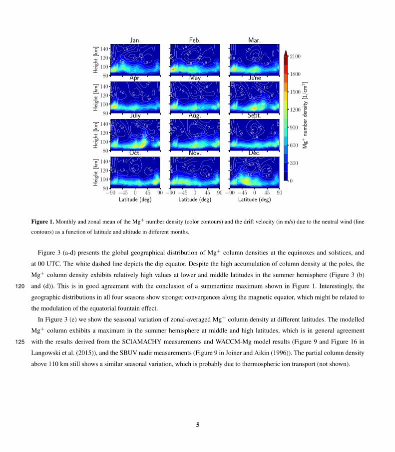
In contrast to the SCIAMACHY measurements, which show a minimum at the equator, the WACCM-X simulation shows a

maximum in peak altitude and number density at the equator. Note that the SCIAMACHY observations are made at a particular

local time of around 10:00 LT, whereas the WACCM-X data in Figure 1 is a diurnal and zonal average. To address this, we also110

present the simulation results at the same local time (10:00 LT) in Figure 2, and they are in better agreement with SCIAMACHY

observations. Another noteworthy feature is that this simulation shows the pronounced maximum in peak altitude and density

at ∼45◦ (N/S) at 10 LT, in accord with the SCIAMACHY observations, which is absent in WACCM-Mg in Langowski et al.

(2015). However, the number densities at 10 LT are even lower, and the peak altitude is about 5 km lower than the daily

averaged simulation ( Figure 1). The pronounced discrepancy between Figure 2 and SCIAMACHY measurements is probably115

due to the diurnal variation of ion electro-dynamical transport, which should be further investigated in the future.

4

80

100

120

140

Hei

ght

[km

]

-5.0

-5.0

-3.0

-3.0

-1.0

-1.0

-1.0

1.0

1.0

1.01.0

3.05.0 Jan.

-5.0 -5.0

-3.0

-3.0-3

.0

-1.0

-1.0-1.0

1.01.0

1.0

3.0

5.0

Feb. -5.0

-3.0 -3.0

-1.0

-1.0

-1.0

1.0

1.0

1.0

Mar.

80

100

120

140

Hei

ght

[km

]

-5.0

-3.0

-3.0

-1.0

-1.0

-1.0

1.0

1.0

1.0

3.0

3.0

Apr.

-5.0

-5.0

-3.0

-3.0

-3.0

-1.0

-1.0-1.0

1.01.0

3.0

3.0

5.0

May

-5.0

-5.0

-5.0

-3.0

-3.0

-3.0

-1.0

-1.0

1.01.0

1.0

3.0

3.0

3.0

5.0June

80

100

120

140

Hei

ght

[km

]

-5.0

-5.0

-5.0

-3.0

-3.0

-3.0

-1.0

-1.0

-1.0

1.01.0

1.0

3.0

3.0

5.0July -5.0 -5.0

-3.0

-3.0

-1.0

-1.0

-1.0

1.0

1.0

3.0

3.0

5.0

Aug. -5.0

-5.0

-3.0

-3.0

-1.0

-1.0

-1.0-1.0

1.0

1.0

1.0

1.0

3.0Sept.

−90 −45 0 45 90Latitude (deg)

80

100

120

140

Hei

ght

[km

]

-5.0

-3.0 -3.0

-1.0

-1.0

-1.0

-1.01.0

1.0

1.01.0

3.0

Oct.

−90 −45 0 45 90Latitude (deg)

-5.0

-5.0

-3.0

-3.0

-3.0-1

.0

-1.0

-1.0

1.0

1.01.0

3.0

5.0

Nov.

−90 −45 0 45 90Latitude (deg)

-5.0-5.0

-5.0-3.0

-3.0

-3.0

-1.0

-1.0-1.0

1.0

1.0

1.01.0

3.0

3.0

5.0 Dec.

0

300

600

900

1200

1500

1800

2100

Mg+

num

ber

dens

ity

[1/c

m3]

Figure 1. Monthly and zonal mean of the Mg+ number density (color contours) and the drift velocity (in m/s) due to the neutral wind (line

contours) as a function of latitude and altitude in different months.

Figure 3 (a-d) presents the global geographical distribution of Mg+ column densities at the equinoxes and solstices, and

at 00 UTC. The white dashed line depicts the dip equator. Despite the high accumulation of column density at the poles, the

Mg+ column density exhibits relatively high values at lower and middle latitudes in the summer hemisphere (Figure 3 (b)

and (d)). This is in good agreement with the conclusion of a summertime maximum shown in Figure 1. Interestingly, the120

geographic distributions in all four seasons show stronger convergences along the magnetic equator, which might be related to

the modulation of the equatorial fountain effect.

In Figure 3 (e) we show the seasonal variation of zonal-averaged Mg+ column density at different latitudes. The modelled

Mg+ column exhibits a maximum in the summer hemisphere at middle and high latitudes, which is in general agreement

with the results derived from the SCIAMACHY measurements and WACCM-Mg model results (Figure 9 and Figure 16 in125

Langowski et al. (2015)), and the SBUV nadir measurements (Figure 9 in Joiner and Aikin (1996)). The partial column density

above 110 km still shows a similar seasonal variation, which is probably due to thermospheric ion transport (not shown).

5

80

100

120

140

Hei

ght

[km

]

Jan. Feb. Mar.

80

100

120

140

Hei

ght

[km

]

Apr. May June

80

100

120

140

Hei

ght

[km

]

July Aug. Sept.

−90 −45 0 45 90Latitude (deg)

80

100

120

140

Hei

ght

[km

]

Oct.

−90 −45 0 45 90Latitude (deg)

Nov.

−90 −45 0 45 90Latitude (deg)

Dec.

0

300

600

900

1200

1500

1800

2100

Mg+

num

ber

dens

ity

[1/c

m3]

Figure 2. Monthly mean Mg+ number density obtained by averaging data at 10 LT for all longitudes as a function of latitude and altitude in

different months.

3.2 Diurnal variations of Mg+ simulated by WACCM-X

To investigate the diurnal variation of metallic ions in the model, we present the Mg+ number density (on a log scale) as a

function of latitude and altitude at the December Solstice and 0◦ longitude; the panels show universal times (i.e. local times) of130

00, 06, 12 and 18 UT (Figure 4 (a-d)). The white dotted line denotes the F2-layer height of the peak electron density (hmF2).

This shows that the strongest diurnal variations are found in equatorial and high latitudes. Here we focus on the “fountain

effect” on ion transport, where the equatorial ions are first lofted to higher altitudes via E×B motion, and then drift down along

the magnetic field lines (Kelley, 2009). Mg+ is expected to be lofted to high altitudes (∼ 400 km) by the E×B drift above the

magnetic equator during the day, because of the daytime eastward electric fields (Huba et al., 2019). Figure 4 (e) shows the135

diurnal variation of Mg+ number density near the dip equator (12◦N, 0◦) as a function of local time; the upward drift of Mg+

peaks at around 20 LT, and the Mg+ then drifts down towards the main layer at midnight (∼ 02 LT). Note that the reduction

of Mg+ at the equator at 06 LT confirms that the ion density at the equator is largely dependent on local time (Figure 4 (b) and

(e)). The phase of Mg+ diurnal variation shows a high correlation with variations in the electron density (the change of hmF2).

Instead of being redistributed along the magnetic field lines to the subtropical region by the “classical” fountain effect (e.g.,140

6

90°E 180° 90°W

45°S

0°

45°N

lati

tude

(a) Mar. Equinox

90°E 180° 90°W

45°S

0°

45°N

(b) June Solstice

90°E 180° 90°WLongitude

45°S

0°

45°N

lati

tude

(c) Sept. Equinox

90°E 180° 90°WLongitude

45°S

0°

45°N

(d) Dec. Solstice

0.0 1.6 3.2 4.8 6.4 8.0 9.6

Column Density [109 atoms cm−2]

Jan Mar May Jul Sep NovMonth

−50

0

50

Lat

itud

e(d

eg)

(e)

0

1

2

3

4

Col

umn

Den

sity

[109

atom

scm−

2]

Figure 3. (a-d) Global geographical distribution of the Mg+ column density during the equinoxes and solstices, at 00 UTC. (e) Seasonal

variation of the zonal mean Mg+ column density as a function of month and latitude. The white dashed lines indicates the position of the dip

equator.

7

Pi et al., 2009), the Mg+ shows a more complex downward trajectory, i.e., the ions are not transported symmetrically to both

sides of the geomagnetic equator, which is closer to the scenario proposed by Cai et al. (2019).

100200300400500

Heig

ht (k

m)

(a) 00 UT (b) 06 UT

90 60 30 0 30 60 90Latitude (deg)

100200300400500

Heig

ht (k

m)

(c) 12 UT

90 60 30 0 30 60 90Latitude (deg)

(d) 18 UT

0 2 4 6 8 10 12 14 16 18 20 22Universal Time (hour)

100200300400500

Heig

ht (k

m)

(e)

0.0 0.5 1.0 1.5 2.0 2.5 3.0 3.5 4.0Mg + Number Density [log10 cm 3]

Figure 4. (a-d) Mg+ density as a function of latitude and altitude at the December Solstice and longitude 0◦, at four universal times (local

times): 00, 06, 12, 18 UT. (e) Mg+ density over (12◦N, 0◦) as a function of universal time and altitude. The white dashed lines denote hmF2.

3.3 Fe and Fe+ vertical profile comparison

In order to demonstrate the effect of electro-dynamical transport on the metals, a standard simulation without metal ion transport

was performed (termed the control run). Figure 5 shows the Fe+ and Fe vertical profiles for the ion transport run (solid lines),145

and control run (dotted/dashed lines) at the equinoxes and solstices. Three geographic latitudes at a longitude of 180◦ are chosen

for comparison: 0◦ for the magnetic equator, 20◦S for the subtropical region corresponding to the fountain effect downward

drift, and 45◦S for the middle latitude corresponding to the summertime peak altitude. Without the ion transport (the control

run), both Fe and Fe+ exhibit roughly Gaussian-shaped layers with peak heights between 90 and 100 km (dotted/dashed lines).

When ion transport is turned on, the vertical profiles of Fe+ vary depending on latitude and season. For instance, Fe+ near150

the equator is always transported to a higher altitude (blue lines), consistent with the fountain effect in the dip equator region.

However, ions at subtropical (20◦S) (orange lines) and middle (45◦S) latitudes (green lines) exhibit quite different transport

motions. At the December solstice at midnight, Fe+ is transported to a high level (∼1 cm−3 at 200-300 km) at middle and

8

subtropical latitudes, which is related to the dominant upward drift velocity due to neutral wind (not shown). In other seasons,

these ions can be transported both upward and downward, depending on the vertical ion velocity.155

Since the neutral atoms are not directly transported by the electromagnetic field, they are influenced by ions through the

recombination between ions and electrons. The last two panels in Figure 5 illustrate the Fe atom distributions. In general,

changes in Fe (at densities > 1 cm−3) do not appear to be synchronized with the upward transport of Fe+, so that the vertical

distribution of Fe in the transport run is similar to that in the control run. However, there is an obvious increase in high-

altitude Fe (i.e. above ∼140 km) in the equatorial region (blue line), corresponding to the upward transport of ions; and at the160

December solstice around midnight, the Fe number density above 150 km is much higher than that in the control run at all

southern latitudes.

3.4 Effect of metal ion mass on transport

Figure 6 compares the Mg+/Fe+ ratio (left panel) and the Mg+/Na+ ratio (right panel) as a function of height and latitude at the

equinoxes and solstices. Note that changes in the ratios below 100 km are due to differences in the ion-molecule chemistries of165

the metals (Plane et al., 2015), which is not the focus here. There are several advantages in choosing these three metallic ions.

First, Fe+ is more than twice as heavy as Mg+. Second, Fe+ is much heavier, and Mg+ is slightly lighter, than the mean mass

of air molecules in the E region. Third, Na+ has a comparable mass with Mg+. As expected, the lighter ions are transported

above 150 km more easily than the heavy Fe+, so that the Mg+/Fe+ ratio increases from ∼1 at 120 km to >2 above 150 km

and to > 30 above 300 km. By the same token, the Mg+/Na+ ratio shows very little change above 120 km.170

The zonally-averaged Fe+/Mg+ ratio below 200 km simulated by WACCM-X also accords with the limited available obser-

vations (Dymond et al., 2003; Kumar and Hanson, 1980), which showed that the average Fe+/Mg+ ratio is around 1.5:1. The

present study also simulates the extreme variability of the Fe+/Mg+ ratio above 300 km (as low as 1:50 in Kumar and Hanson

(1980)). However, the unexpectedly large Fe+/Mg+ ratio (∼10–50) reported by Dymond et al. (2003) is only captured at a few

points about 150 km in our model (not shown). Interestingly, the striking differences between distinct thermosphere-ionosphere175

Fe and diffuse thermosphere-ionosphere Na reported by Chu et al. (2020) are thought to be related to mass separation. There

is no question that more observations are needed to confirm and validate these findings.

Figure 6 shows that whereas the Mg+/Fe+ ratios (left panel) show relatively little latitudinal variation compared with the

variation with altitude (mostly caused by the mass difference of the ions), the Mg+/Na+ ratios (right panel) show marked

interhemispheric differences at the solstice periods. The reason for this is the difference in the ion-molecule chemistry of Na+,180

compared with Mg+ (and Fe+). The Na+ ion has a closed electronic shell (it is isoelectronic with the inert gas Ne), and so

does not react with O3, in contrast to Mg+ and Fe+ (Plane et al., 2015). Formation of MgO+ by the fast reaction with O3 is

the main route to neutralization of Mg+ above 90 km (Whalley et al., 2011). During summer at mid- to high-latitudes (> 30◦),

O3 above 90 km is heavily depleted through a combination of longer diurnal photolysis and reaction with the elevated levels

of H produced from H2O which upwells over the summer pole (Plane et al., 2015). In contrast, the O3 density in the lower185

thermosphere is more than an order of magnitude higher in the winter polar vortex. The result is that lower thermospheric

Mg+ ions at latitudes higher than ∼30◦ are relatively long-lived in summer, and can be transported vertically throughout the

9

100

150

200

250

300

350H

eigh

t[k

m]

Fe+, Mar. Equinox, 12 LTFe+, Mar. Equinox, 00 LT Fe, Mar. Equinox, 12 LT Fe, Mar. Equinox, 00 LT

100

150

200

250

300

350

Hei

ght

[km

]

Fe+, June Solstice, 12 LT Fe+, June Solstice, 00 LT Fe, June Solstice, 12 LT Fe, June Solstice, 00 LT

100

150

200

250

300

350

Hei

ght

[km

]

Fe+, Sept. Equinox, 12 LTFe+, Sept. Equinox, 00 LTFe, Sept. Equinox, 12 LT Fe, Sept. Equinox, 00 LT

10−1 101 103100 102 104

Concentration [1/cm3]

100

150

200

250

300

350

Hei

ght

[km

]

Fe+, Dec. Solstice, 12 LT

10−1 101 103100 102 104

Concentration [1/cm3]

Fe+, Dec. Solstice, 00 LT

10−1 101 103100 102 104

Concentration [1/cm3]

Fe, Dec. Solstice, 12 LT

10−1 101 103100 102 104

Concentration [1/cm3]

Fe, Dec. Solstice, 00 LT

(180◦,0◦) Transport Run

(180◦,0◦) Control Run

(180◦,20◦S) Transport Run

(180◦,20◦S) Control Run

(180◦,45◦S) Transport Run

(180◦,45◦S) Control Run

Figure 5. Comparison of the vertical profiles of the Fe+ (left two panels) and Fe (right two panels) number densities, for the control run

(dotted/dashed lines) and run with ion transport (solid lines) over selected geographic latitudes, at the equinoxes and solstices and midday

(12 LT) and midnight (00 LT).

10

thermosphere. This leads to the higher Mg+/Na+ ratios in the summer hemisphere, as shown in Figure 6. The converse operates

at latitude higher than 30◦ in the winter hemisphere, where the relatively high O3 tends to neutralize lower thermospheric Mg+.

Because Na+ and Mg+ have very similar masses, their ratios above 100 km are fairly constant with height.190

100

150

200

250

300H

eigh

t[k

m]

log10(Mg+/Fe+), Mar. Equinox log10(Mg+/Na+), Mar. Equinox

100

150

200

250

300

Hei

ght

[km

]

log10(Mg+/Fe+), June Solstice log10(Mg+/Na+), June Solstice

100

150

200

250

300

Hei

ght

[km

]

log10(Mg+/Fe+), Sept. Equinox log10(Mg+/Na+), Sept. Equinox

−90 −60 −30 0 30 60 90Latitude (deg)

100

150

200

250

300

Hei

ght

[km

]

log10(Mg+/Fe+), Dec. Solstice

−90 −60 −30 0 30 60 90Latitude (deg)

log10(Mg+/Na+), Dec. Solstice

−2.0

−1.5

−1.0

−0.5

0.0

0.5

1.0

1.5

Figure 6. The zonally-averaged Mg+/Fe+ ratio (left panel) and Mg+/Na+ ratio (right panel) versus height and latitude at the equinoxes and

solstices.

3.5 Effect of NO+ and O+2 transport

Figure 7 and 8 compare the distribution of metal ions from two simulations, one with the transport of all ions (hereafter TA),

and the other with NO+ and O+2 in chemical equilibrium (hereafter CE). Note that the simulation results presented herein

investigate the potential impacts of the transport of two major molecular ions on the distribution of metallic ions and do not

provide a comprehensive review of all possible effects.195

11

Figure 7 shows the monthly mean density of Mg+ as a function of latitude and altitude in June for the TA (Figures 7a)

and CE (Figures 7b) simulations, along with their difference (Figures 7c), where the monthly mean data is zonally averaged.

In general, there is a good correspondence between the two simulations in terms of the latitude-altitudinal distribution of the

monthly mean Mg+ density. As seen in Figure 7c, the peak density in CE simulation is generally a little higher than that in

the TA simulation, especially in the high latitudes of the southern hemisphere. Figure 8 compares the diurnal variation of Mg+200

in the two simulations. Both cases simulate the significant “fountain effect”, which was discussed in Section 3.2. With the

transport of major molecular ions, the peak height of the metal layer after midnight is higher. As discussed by Plane et al.

(2015), the charge transfer of neutral metal atoms with NO+ and O+2 is the major sources of metallic ions in the E region. Due

to the very short lifetimes of NO+ and O+2 during daytime, the transport of these molecular ions between model grid-boxes

has little effect on the metallic ions. In contrast, the reduced densities of the molecular ions (and electrons) at night means that205

their increased lifetimes become comparable to transport time-step. Additional metallic ions are therefore produced via charge

transfer with the downward transport of NO+ and O+2 at night in the TA simulation.

4 Conclusions

The WACCM-X high altitude chemistry-climate model has been extended to incorporate the full life cycle of multiple me-

teoric metal ions and atoms (Mg, Na, and Fe, currently). A major advantage of WACCM-X is the self-consistent treatment210

of dynamics and electrodynamics allowing us to quantitatively investigate the global distribution of metal ions and the for-

mation mechanisms of thermospheric metal layers. The present study explores, for the first time, the seasonal variations of

thermospheric metal ions by including global metal ion transport in the E and F regions.

There are a number of interesting findings: (1) A clear seasonal cycle is found in the monthly averaged global distributions

of Mg+, in good agreement with the SCIAMACHY measurements (Langowski et al., 2015), although the peak height and peak215

density are about 5 km and 35% lower than the observations, respectively. (2) Uplift of metal ions in the summer hemisphere

at mid-latitudes (∼ 40◦±10◦), driven by the vertical ion velocity due to the neutral wind, appears to explain the summer peak

occurrence of lower thermospheric neutral Na layers observed by mid-latitude lidars (Wang et al., 2012; Dou et al., 2013;

Yuan et al., 2014; Xun et al., 2020). (3) Upward transport of metallic ions by E×B forcing is generally consistent with the

“fountain effect”. (4) The formation of thermospheric neutral metal layers is strongly influenced by the upward transport of220

ions, since metallic atoms and ions are coupled by relatively fast reactions in the lower thermosphere (Plane et al., 2015). (5)

A pronounced mass separation of Fe+ with the two lighter ions, Mg+ and Na+, is demonstrated above 150 km, with the ratio

between the lighter ions (Mg+ and Na+) and heavier ions (Fe+) increasing with height by more than a factor of 2 above 150

km. More satellite observations of the Mg+/Fe+ ratio are needed to test this prediction. (6) The role of NO+ and O+2 transport

in the distribution of metal ions in the model is examined by comparing the two simulation results. It is found that they have225

little effect on the monthly means of metal ions but affect the peak heights of metallic ions in the descending phase of the

“fountain effect”.

12

80

100

120

140

Hei

ght

[km

]

(a)

80

100

120

140

Hei

ght

[km

]

(b)

−90 −60 −30 0 30 60 90Latitude (deg)

80

100

120

140

Hei

ght

[km

]

(c)

0

300

600

900

1200

1500

1800

2100

Mg+

num

ber

dens

ity

[1/c

m3]

−120−60060120180240300360420

Mg+

num

ber

dens

ity

[1/c

m3]

Figure 7. The monthly and zonal mean of the Mg+ number density in June from (a) the TA simulation and (b) the CE simulation. (c) The

difference between the TA and CE simulations.

13

0 2 4 6 8 10 12 14 16 18 20 22Universal Time (hour)

100

200

300

400

500

Heig

ht (k

m)

(a)

0 2 4 6 8 10 12 14 16 18 20 22Universal Time (hour)

(b)

0.0 0.5 1.0 1.5 2.0 2.5 3.0 3.5 4.0Mg + Number Density [log10 cm 3]

Figure 8. Mg+ density over (12◦N, 0◦, near the dip equator) as a function of universal time and altitude at June Solstice. The dashed lines

denote hmF2. (a) for the TA simulation and (b) for the CE simulation.

Previous research has established that thermospheric neutral metal layers are modulated by dynamics (e.g. gravity waves,

atmospheric tides) (e.g., Chu et al., 2011; Xue et al., 2013; Liu et al., 2016; Cai et al., 2017; Qiu et al., 2016; Chu et al., 2020).

In the future, this new version of WACCM-X can be used to better investigate the effect of lower atmospheric dynamical230

processes on the formation of thermospheric neutral metal layers, by using the “specified-dynamics” version of the model

(SD-WACCM-X).

Code and data availability. As a part of CESM2, WACCM-X is available at http://www.cesm.ucar.edu/models/cesm2/.

Author contributions. JW, WF, HL, and JMCP designed the simulations and wrote the manuscript. XX and DRM contributed to the discus-

sion and explanation of model simulations. All authors discussed the results and commented on the manuscript at all stages.235

Competing interests. The authors declare that they have no conflict of interest.

Acknowledgements. This work was supported by the B-type Strategic Priority Program of the Chinese Academy of Sciences (Grant No.

XDB41000000), the National Natural Science Foundation of China (42074181, 41774158, 41831071, 41804147, and 41704148), and the

Open Research Project of Large Research Infrastructures of CAS “Study on the interaction between low/midatitude atmosphere and iono-

14

sphere based on the Chinese Meridian Project.” . J. W. was funded by the Joint Open Fund of Mengcheng National Geophysical Observatory240

(No. MENGO-202008). W. F. and J. M. C. P. were funded by the European Research Council CODITA project (291332). HLL acknowl-

edges partial support by NSF OPP 1443726. National Center for Atmospheric Research is a major facility sponsored by the National Science

Foundation under Cooperative Agreement No. 1852977. The numerical calculations in this paper were in part undertaken on the supercom-

puting system in the Supercomputing Center of University of Science and Technology of China, and ARC3, part of the High Performance

Computing facilities at the University of Leeds.245

15

References

Bones, D. L., Plane, J. M. C., and Feng, W.: Dissociative Recombination of FeO+ with Electrons: Implications for Plasma Layers in the

Ionosphere, The Journal of Physical Chemistry A, 120, 1369–1376, https://doi.org/10.1021/acs.jpca.5b04947, 2016.

Boris, J., Landsberg, A., Oran, E., and Gardner, J.: LCPFCT-A Flux-Corrected Transport Algorithm for Solving Generalized Continuity

Equations, NRL Memorandum Report, pp. 93–7192, 1993.250

Cai, X., Yuan, T., and Eccles, J. V.: A Numerical Investigation on Tidal and Gravity Wave Contributions to the Summer Time Na Variations in

the Midlatitude E Region, Journal of Geophysical Research: Space Physics, 122, 10,577–10,595, https://doi.org/10.1002/2016JA023764,

2017.

Cai, X., Yuan, T., Eccles, J. V., Pedatella, N. M., Xi, X., Ban, C., and Liu, A. Z.: A Numerical Investigation on the Variation of Sodium Ion

and Observed Thermospheric Sodium Layer at Cerro Pachón, Chile During Equinox, Journal of Geophysical Research: Space Physics,255

124, 10 395–10 414, https://doi.org/10.1029/2018JA025927, 2019.

Carrillo-Sánchez, J. D., Gómez-Martín, J. C., Bones, D. L., Nesvorný, D., Pokorný, P., Benna, M., Flynn, G. J., and Plane, J. M.: Cosmic

dust fluxes in the atmospheres of Earth, Mars, and Venus, Icarus, 335, 113 395, https://doi.org/10.1016/j.icarus.2019.113395, 2020.

Carter, L. N. and Forbes, J. M.: Global transport and localized layering of metallic ions in the upper atmospherer, Annales Geophysicae, 17,

190–209, https://doi.org/10.1007/s00585-999-0190-6, 1999.260

Chu, X. and Yu, Z.: Formation mechanisms of neutral Fe layers in the thermosphere at Antarctica studied with a thermosphere-ionosphere

Fe/Fe+(TIFe) model, Journal of Geophysical Research: Space Physics, 122, 6812–6848, https://doi.org/10.1002/2016JA023773, 2017.

Chu, X., Yu, Z., Gardner, C. S., Chen, C., and Fong, W.: Lidar observations of neutral Fe layers and fast gravity waves in the thermosphere

(110-155 km) at McMurdo (77.8°S, 166.7°E), Antarctica, Geophysical Research Letters, 38, https://doi.org/10.1029/2011GL050016,

2011.265

Chu, X., Nishimura, Y., Xu, Z., Yu, Z., Plane, J. M. C., Gardner, C. S., and Ogawa, Y.: First Simultaneous Lidar Observations

of Thermosphere-Ionosphere Fe and Na (TIFe and TINa) Layers at McMurdo (77.84°S, 166.67°E), Antarctica With Concurrent

Measurements of Aurora Activity, Enhanced Ionization Layers, and Converging Electric Field, Geophysical Research Letters, 47,

e2020GL090 181, https://doi.org/10.1029/2020GL090181, 2020.

Dou, X. K., Qiu, S. C., Xue, X. H., Chen, T. D., and Ning, B. Q.: Sporadic and thermospheric enhanced sodium layers observed by a lidar270

chain over China, Journal of Geophysical Research: Space Physics, 118, 6627–6643, https://doi.org/10.1002/JGRA.50579, 2013.

Dymond, K. F., Wolfram, K. D., Budzien, S. A., Nicholas, A. C., McCoy, R. P., and Thomas, R. J.: Middle ultraviolet emission from ionized

iron, Geophysical Research Letters, 30, 1003, https://doi.org/10.1029/2002GL015060, 2003.

Feng, W. H., Marsh, D. R., Chipperfield, M. P., Janches, D., Hoffner, J., Yi, F., and Plane, J. M. C.: A global atmospheric model of meteoric

iron, Journal of Geophysical Research-Atmospheres, 118, 9456–9474, 2013.275

Friedman, J. S., Chu, X., Brum, C. G. M., and Lu, X.: Observation of a thermospheric descending layer of neutral K over Arecibo, Journal

of Atmospheric and Solar-Terrestrial Physics, 104, 253–259, https://doi.org/10.1016/j.jastp.2013.03.002, 2013.

Gao, Q., Chu, X., Xue, X., Dou, X., Chen, T., and Chen, J.: Lidar observations of thermospheric Na layers up to 170 km with

a descending tidal phase at Lijiang (26.7°N, 100.0°E), China, Journal of Geophysical Research: Space Physics, 120, 9213–9220,

https://doi.org/10.1002/2015JA021808, 2015.280

Huba, J. D., Krall, J., and Drob, D.: Global Ionospheric Metal Ion Transport With SAMI3, Geophysical Research Letters, 46, 7937–7944,

https://doi.org/10.1029/2019GL083583, 2019.

16

Hurrell, J. W., Holland, M. M., Gent, P. R., Ghan, S., Kay, J. E., Kushner, P. J., Lamarque, J.-F., Large, W. G., Lawrence, D., Lindsay, K.,

Lipscomb, W. H., Long, M. C., Mahowald, N., Marsh, D. R., Neale, R. B., Rasch, P., Vavrus, S., Vertenstein, M., Bader, D., Collins, W. D.,

Hack, J. J., Kiehl, J., and Marshall, S.: The Community Earth System Model: A Framework for Collaborative Research, Bulletin of the285

American Meteorological Society, 94, 1339 – 1360, https://doi.org/10.1175/BAMS-D-12-00121.1, 2013.

Joiner, J. and Aikin, A. C.: Temporal and spatial variations in upper atmospheric Mg+, Journal of Geophysical Research: Space Physics,

101, 5239–5249, https://doi.org/10.1029/95JA03517, 1996.

Kelley, M.: The Earth’s Ionosphere: Plasma Physics and Electrodynamics (2nd ed.), Elsevier, Academic Press, London WC1X 8RR, UK,

2009.290

Kumar, S. and Hanson, W. B.: The morphology of metallic ions in the upper atmosphere, Journal of Geophysical Research, 85, 6783–6801,

https://doi.org/10.1029/JA085iA12p06783, 1980.

Langowski, M. P., von Savigny, C., Burrows, J. P., Feng, W., Plane, J. M. C., Marsh, D. R., Janches, D., Sinnhuber, M., Aikin, A. C., and

Liebing, P.: Global investigation of the Mg atom and ion layers using SCIAMACHY/Envisat observations between 70 and 150 km altitude

and WACCM-Mg model results, Atmospheric Chemistry and Physics, 15, 273–295, https://doi.org/10.5194/ACP-15-273-2015, 2015.295

Layzer, D.: Theory of Midlatitude Sporadic E, Radio Science, 7, 385–395, https://doi.org/10.1029/RS007i003p00385, 1972.

Liu, A. Z., Guo, Y., Vargas, F., and Swenson, G. R.: First measurement of horizontal wind and temperature in the lower

thermosphere (105–140 km) with a Na Lidar at Andes Lidar Observatory, Geophysical Research Letters, 43, 2374–2380,

https://doi.org/10.1002/2016GL068461, 2016.

Liu, H., Foster, B. T., Hagan, M. E., McInerney, J. M., Maute, A., Qian, L., Richmond, A. D., Roble, R. G., Solomon, S. C., Garcia, R. R.,300

Kinnison, D., Marsh, D. R., Smith, A. K., Richter, J., Sassi, F., and Oberheide, J.: Thermosphere extension of the Whole Atmosphere Com-

munity Climate Model, Journal of Geophysical Research: Space Physics, 115, A12 302, https://doi.org/10.1029/2010JA015586, 2010.

Liu, H., Bardeen, C. G., Foster, B. T., Lauritzen, P., Liu, J., Lu, G., Marsh, D. R., Maute, A., McInerney, J. M., Pedatella, N. M., Qian,

L., Richmond, A. D., Roble, R. G., Solomon, S. C., Vitt, F. M., and Wang, W.: Development and Validation of the Whole Atmosphere

Community Climate Model With Thermosphere and Ionosphere Extension (WACCM-X 2.0), Journal of Advances in Modeling Earth305

Systems, 10, 381–402, https://doi.org/10.1002/2017MS001232, 2018a.

Liu, J., Liu, H., Wang, W., Burns, A. G., Wu, Q., Gan, Q., Solomon, S. C., Marsh, D. R., Qian, L., Lu, G., Pedatella, N. M., McInerney, J. M.,

Russell, J. M., and Schreiner, W. S.: First Results From the Ionospheric Extension of WACCM-X During the Deep Solar Minimum Year

of 2008, Journal of Geophysical Research: Space Physics, 123, 1534–1553, https://doi.org/10.1002/2017JA025010, 2018b.

Marsh, D. R., Janches, D., Feng, W. H., and Plane, J. M. C.: A global model of meteoric sodium, Journal of Geophysical Research-310

Atmospheres, 118, 11 442–11 452, 2013a.

Marsh, D. R., Mills, M. J., Kinnison, D. E., Lamarque, J. F., Calvo, N., and Polvani, L. M.: Climate Change from 1850 to 2005 Simulated in

CESM1(WACCM), Journal of Climate, 26, 7372–7391, https://doi.org/10.1175/JCLI-D-12-00558.1, 2013b.

Narcisi, R. S.: Processes associated with metal-ion layers in the E region of the ionosphere, Space Research, 8, 360–369, 1968.

Neale, R. B., Richter, J., Park, S., Lauritzen, P. H., Vavrus, S. J., Rasch, P. J., and Zhang, M. H.: The Mean Climate of the Community Atmo-315

sphere Model (CAM4) in Forced SST and Fully Coupled Experiments, Journal of Climate, 26, 5150–5168, https://doi.org/10.1175/JCLI-

D-12-00236.1, 2013.

Pi, X. Q., Mannucci, A. J., Iijima, B. A., Wilson, B. D., Komjathy, A., Runge, T. F., and Akopian, V.: Assimilative Modeling of Ionospheric

Disturbances with FORMOSAT-3/COSMIC and Ground-Based GPS Measurements, Terrestrial Atmospheric and Oceanic Sciences, 20,

273–285, https://doi.org/10.3319/Tao.2008.01.04.01(F3c), 2009.320

17

Plane, J. M. C., Feng, W., and Dawkins, E. C.: The mesosphere and metals: chemistry and changes, Chemical Reviews, 115, 4497–541,

https://doi.org/10.1021/cr500501m, 2015.

Qiu, S. C., Tang, Y. H., Jia, M. J., Xue, X. H., Dou, X. K., Li, T., and Wang, Y. H.: A review of latitudinal characteris-

tics of sporadic sodium layers, including new results from the Chinese Meridian Project, Earth-Science Reviews, 162, 83–106,

https://doi.org/10.1016/j.earscirev.2016.07.004, 2016.325

Schunk, R. W. and Nagy, A. F.: Simplified Transport Equations, p. 104–147, Cambridge Atmospheric and Space Science Series, Cambridge

University Press, https://doi.org/10.1017/CBO9780511551772.005, 2000.

Viehl, T. P., Plane, J. M. C., Feng, W., and Höffner, J.: The photolysis of FeOH and its effect on the bottomside of the mesospheric Fe layer,

Geophysical Research Letters, 43, 1373–1381, https://doi.org/10.1002/2015GL067241, 2016.

Wang, J., Yang, Y., Cheng, X., Yang, G., Song, S., and Gong, S.: Double sodium layers observation over Beijing, China, Geophysical330

Research Letters, 39, https://doi.org/10.1029/2012GL052134, 2012.

Whalley, C. L., Martín, J. C. G., Wright, T. G., and Plane, J. M. C.: A kinetic study of Mg+ and Mg-containing ions reacting with O3, O2,

N2, CO2, N2O and H2O: implications for magnesium ion chemistry in the upper atmosphere, Phys. Chem. Chem. Phys., 13, 6352–6364,

https://doi.org/10.1039/C0CP02637A, 2011.

Xue, X. H., Dou, X. K., Lei, J., Chen, J. S., Ding, Z. H., Li, T., Gao, Q., Tang, W. W., Cheng, X. W., and Wei, K.: Lower thermospheric-335

enhanced sodium layers observed at low latitude and possible formation: Case studies, Journal of Geophysical Research: Space Physics,

118, 2409–2418, https://doi.org/10.1002/JGRA.50200, 2013.

Xun, Y., Yang, G., Wang, J., Du, L., Wang, Z., Jiao, J., Cheng, X., Li, F., and Zou, X.: The Comprehensive Study of Low Thermospheric

Sodium Layers during the 24th Solar Cycle, Atmosphere, 11, 284, 2020.

Yu, B., Xue, X., Scott, C. J., Wu, J., Yue, X., Feng, W., Chi, Y., Marsh, D. R., Liu, H., Dou, X., and Plane, J. M. C.: Interhemispheric transport340

of metallic ions within ionospheric sporadic E layers by the lower thermospheric meridional circulation, Atmospheric Chemistry and

Physics, 21, 4219–4230, https://doi.org/10.5194/acp-21-4219-2021, 2021.

Yuan, T., Wang, J., Cai, X., Sojka, J., Rice, D., Oberheide, J., and Criddle, N.: Investigation of the seasonal and local time variations of

the high-altitude sporadic Na layer (Nas) formation and the associated midlatitude descending E layer (Es) in lower E region, Journal of

Geophysical Research: Space Physics, 119, 5985–5999, https://doi.org/10.1002/2014JA019942, 2014.345

18