Selection on moral hazard in health insurance�

Liran Einav, Amy Finkelstein, Stephen Ryan, Paul Schrimpf, and Mark Culleny

March 2012

We use employee-level panel data from a single �rm to explore the possibility that

individuals may select insurance coverage in part based on their anticipated behavioral

(�moral hazard�) response to insurance, a phenomenon we label �selection on moral

hazard.�Using a model of plan choice and medical utilization, we present evidence of

heterogeneous moral hazard as well as selection on it, and explore some of its implica-

tions. For example, we show that, at least in our context, abstracting from selection

on moral hazard could lead to over-estimates of the spending reduction associated with

introducing a high-deductible health insurance option.

JEL classi�cation numbers: D12, D82, G22

Keywords: Insurance markets; Adverse selection; Moral hazard; Health insurance

�We are grateful to Felicia Bayer, Brenda Barlek, Chance Cassidy, Fran Filpovits, Frank Patrick, and Mike

Williams for innumerable conversations explaining the institutional environment of Alcoa, to Colleen Barry, Susan

Busch, Linda Cantley, Deron Galusha, James Hill, Sally Vegso, and especially Marty Slade for providing and explain-

ing the data, to Tatyana Deryugina, Sean Klein, Michael Powell, Iuliana Pascu, and James Wang for outstanding

research assistance, and to Ben Handel, Justine Hastings, Jim Heckman, Igal Hendel, Nathan Hendren, Kate Ho,

Pat Kline, Jon Levin, Matt Notowidigdo, Phil Reny, Rob Townsend, numerous seminar participants, four anonymous

refrerees, and Penny Goldberg (the Editor) for helpful comments and suggestions. The data were provided as part

of an ongoing service and research agreement between Alcoa, Inc. and Stanford, under which Stanford faculty, in

collaboration with faculty and sta¤ at Yale University, perform jointly agreed-upon ongoing and ad hoc research

projects on workers�health, injury, disability, and health care, and Mark Cullen serves as Senior Medical Advisor

for Alcoa, Inc. We gratefully acknowledge support from the NIA (R01 AG032449), the National Science Foundation

Grant SES-0643037 (Einav), the Alfred P. Sloan Foundation (Finkelstein), the John D. and Catherine T. MacArthur

Foundation Network on Socioeconomic Status and Health, and Alcoa, Inc. (Cullen), and the U.S. Social Security

Administration through grant #5 RRC08098400-03-00 to the National Bureau of Economic Research as part of the

SSA Retirement Research Consortium. Einav also acknowledges the hospitality of the Center for Advanced Study in

the Behavioral Sciences at Stanford. The �ndings and conclusions expressed are solely those of the authors and do

not represent the views of SSA, any agency of the Federal Government, or the NBER.yEinav: Department of Economics, Stanford University, and NBER, leinav@stanford.edu; Finkelstein: Department

of Economics, MIT, and NBER, a�nk@mit.edu; Ryan: Department of Economics, MIT, and NBER, sryan@mit.edu;

Schrimpf: Department of Economics, UBC, schrimpf@mail.ubc.ca; Cullen: Department of Internal Medicine, School

of Medicine, Stanford University, and NBER, mrcullen@stanford.edu.

Economic analysis of market failure in insurance markets tends to analyze selection and moral

hazard as distinct phenomena. In this paper, we explore the potential for selection on moral hazard

in insurance markets. By this we mean the possibility that moral hazard e¤ects are heterogeneous

across individuals, and that individuals� selection of insurance coverage is a¤ected by their an-

ticipated behavioral response to coverage. We examine these issues empirically in the context of

employer-provided health insurance in the United States. Speci�cally, we break down the general

problem of adverse selection to two components: one is driven by the �traditional�selection on the

level of expected health risk, while the other is driven by slope of spending, namely the incremental

medical utilization that is due to greater insurance coverage, which we refer to as �moral hazard.�

Such selection on moral hazard has implications for the standard analysis of both selection and

moral hazard. For example, a standard approach to in�uence selection in insurance markets is risk

adjustment, i.e. pricing on observable characteristics that predict one�s insurance claims. However,

the potential for selection on moral hazard suggests that monitoring techniques that are usually

thought of as reducing moral hazard �such as cost sharing that varies across categories of claims

with di¤erential scope for behavioral response �may also have important bene�ts in combatting

adverse selection. In contrast, a standard approach to in�uence moral hazard is to o¤er plans

with higher consumer cost sharing. But if individuals�anticipated behavioral response to coverage

a¤ects their propensity to select such plans, the magnitude of the behavioral response could be

much lower (or much higher) from what would be achieved if plan choices were unrelated to the

behavioral response. As we discuss in more detail below, not only the existence of selection on

moral hazard but also the sign of any relationship between anticipated behavioral response and

demand for higher coverage is ex ante ambiguous. Ultimately, these are open empirical questions.

Health insurance provides a particularly interesting setting in which to explore these issues.

Both selection and moral hazard have been well-documented in the context of employer-provided

health insurance. Moreover, given the extensive government involvement in health insurance, as

well as the concern about the size and rapid growth of the healthcare sector, there is considerable

academic and public policy interest in a better understanding of selection and moral hazard in this

context.

Recognition of the possibility of selection on moral hazard, however, highlights potentially

important limitations of analyzing these problems in isolation. For example, the sizable empirical

literature on the likely spending reductions that could be achieved through higher consumer cost

sharing has intentionally focused on isolating and exploring exogenous changes in cost sharing,

such as those induced by the famous RAND experiment (Manning et al., 1987; Newhouse, 1993).

Yet, the very same feature that solves the causal inference problem �namely randomization (or

attempts to approximate it in the subsequent quasi-experimental literature on this topic) �removes

the endogenous choice element. It thus abstracts, by design, from any selection on moral hazard,

which could have important implications for the spending reductions achieved through o¤ering

plans with higher consumer cost sharing. This is particularly relevant since substantial plan choice

is now the norm not only in private health insurance but also increasingly in public health insurance

programs, such as Medicare Part D.

1

We begin by presenting a utility-maximizing model of individual health insurance plan choices

and subsequent healthcare spending. The model characterizes individuals as associated with two

distinct risk attributes: a �level� and a �slope.� The former refers to their health risk, or their

expected level of healthcare spending without insurance. The latter captures the incremental

healthcare spending from insurance coverage (i.e., the slope of healthcare spending with respect to

its out-of-pocket price). The use of the term moral hazard is far from standard in the literature,

and the model allows us to be precise as to what we mean by it. We de�ne moral hazard as the

slope of healthcare spending (with respect to price), and by �selection on moral hazard�we refer to

the component of adverse selection that is driven by heterogeneity in this slope parameter. In other

words, while traditional models of adverse selection focus on heterogeneity in (and selection on)

the level of expected medical utilization, we emphasize that adverse selection could also be driven

by selection on the slope of medical spending with respect to its price. That is, greater coverage

would be more attractive for individuals whose healthcare utilization would increase more sharply

in response to this coverage, thus generating greater cost to the insurance company.

We explore these issues empirically in the speci�c setting of the U.S. employees at Alcoa Inc., a

large multinational producer of aluminum and related products. Naturally, as we emphasize below,

this makes our quantitative results speci�c to our setting. We have individual-level panel data

on the health insurance options, choices, and subsequent medical utilization of Alcoa�s employees

(and their covered dependents). Crucially for identifying and estimating moral hazard, we observe

variation in the health insurance options o¤ered to di¤erent groups of workers at di¤erent points

of time stemming from staggered timing of new union contracts. We present descriptive and

motivating di¤erence-in-di¤erences estimates on moral hazard in our setting, as well as patterns

that may be suggestive of heterogeneity in and selection on this moral hazard e¤ect.

In order to formalize the analysis of selection on moral hazard and to explore some of its im-

plications, we embed the economic model of coverage choice and healthcare spending within an

econometric model that allows for unobserved heterogeneity across individuals along three dimen-

sions �health expectations, risk aversion, and moral hazard �and for �exible correlation across

these three. All else equal, willingness to pay for coverage is increasing in the individual�s health

expectation and his risk aversion; these are standard results. In addition, in our model, willing-

ness to pay for coverage is increasing in the individual�s moral hazard: individuals with a greater

behavioral response to coverage bene�t more from greater coverage, since they will consume more

care as a result. This is the selection on moral hazard comparative static that is the focus of our

paper. Empirically, however, the sign (let alone the magnitude) of any selection on moral hazard is

ambiguous and depends on the extent of heterogeneity in moral hazard as well as the correlation

between moral hazard and the other primitives that a¤ect health insurance choice, expected health

and risk aversion. We use this model and the data to recover the joint distribution of individuals�

(unobserved) health, risk aversion, and moral hazard. The model is estimated using Markov Chain

Monte Carlo Gibbs sampler, and its �t appears reasonable.

Qualitatively, we �nd that individuals who exhibit a greater behavioral response to coverage are

more likely to choose higher coverage plans. Quantitatively, we estimate substantial heterogeneity

2

in moral hazard and selection on it. We focus on the counterfactual of moving from the most

comprehensive to the least comprehensive of the new options �essentially moving individuals from

a no-deductible plan to a high ($3,000 for family coverage) deductible plan. In terms of heterogeneity

in moral hazard, we �nd that the standard deviation across individuals of the spending reduction

from this change in plans is more than twice the average. In terms of selection on moral hazard, we

�nd that for determining the choice between these two plans, selection on moral hazard is roughly

as important as selection on health risk, and considerably more important than selection on risk

aversion.

We use the model to examine some of the implications of the selection on moral hazard we

detect. For example, our results suggest that the spending reduction associated with introducing a

high-deductible plan could be substantially lower than what would be predicted if we were to ignore

selection on moral hazard and assume that those who choose the high-deductible plan are randomly

drawn. This is a direct consequence of our �nding that those who select less comprehensive coverage

are likely to exhibit a smaller behavioral response to the insurance coverage.

Our paper is related to several distinct literatures. Our modeling approach is closely related

to that of Cardon and Hendel (2001), which is also the approach taken by Bajari et al. (2010),

Carlin and Town (2010), and Handel (2011) in modeling health insurance plan choice. Like us, all

of these papers have allowed for selection based on expected health risk. Our paper di¤ers in our

focus on identifying and estimating moral hazard �and in particular heterogeneous moral hazard �

and in examining the relationship between moral hazard and plan choice. From a methodological

perspective, we also di¤er from these and many other discrete choice models in that we do not allow

for a choice-speci�c, i.i.d. error term, which does not seem appealing given the vertically rankable

nature of our choices.

Our di¤erence-in-di¤erences analysis of the spending reduction associated with changes in cost

sharing is related to a sizable experimental and quasi-experimental literature in health economics

analyzing the impact of higher consumer cost sharing on spending (see Chandra, Gruber and

McKnight (2010) for a recent review). However, our subsequent exploration of heterogeneity in

this average moral hazard e¤ect and selection on it suggests the need for caution in using such

estimates, which do not account for endogenous plan selection, for forecasting the likely spending

e¤ects of introducing the option of plans with higher consumer cost sharing. It also suggests that

one can embed the basic identi�cation approach of the di¤erence-in-di¤erences framework in a

model that allows for and investigates such endogenous selection.

Our examination of selection on moral hazard is motivated in part by the growing empirical

literature demonstrating that focusing on selection that is driven by one-dimensional heterogeneity

in risk, as in the early seminal theoretical contributions to the topic, may miss many interesting

aspects of actual markets. This literature has tended to abstract from moral hazard, and focused on

selection on preferences, such as risk aversion (Finkelstein and McGarry, 2006; Cohen and Einav,

2007), cognition (Fang, Keane, and Silverman, 2008), or desire for wealth after death (Einav, Finkel-

stein, and Schrimpf, 2010). Our exploration highlights another potential dimension of selection,

and one that has particularly interesting implications for contract design (in contexts where moral

3

hazard is important). While there are questions for which the extent to which selection occurs on

the basis of expected health or moral hazard does not matter (see, e.g., Einav, Finkelstein, and

Cullen, 2010), we illustrate in this paper that breaking down selection to �selection on levels�and

�selection on slopes�can be important for answering questions regarding the design of contracts to

reduce selection and the implications of contract design for spending.

Despite its potential importance, we are not aware of any empirical work attempting to iden-

tify and analyze selection on moral hazard in insurance markets. The basic idea of selection on

moral hazard, however, is not unique to us. Similar ideas have appeared in several other contexts.1

Indeed, one general way to think about the concept of selection on moral hazard is in the con-

text of estimating a treatment e¤ect of insurance coverage on medical expenditure. As we already

hinted, within such a framework selection on health risk would be equivalent to heterogeneity in

(and selection on) the level (or constant term in a regression of medical spending on insurance

coverage), while selection on moral hazard can be thought of as heterogeneity in (and selection on)

the slope coe¢ cient. Heckman, Urzua and Vytlacil (2006) present an econometric examination of

the properties of IV estimators when individuals select into treatment in part based on their an-

ticipated response to the treatment, a phenomenon they refer to as �essential heterogeneity.�They

subsequently apply these ideas in the context of the returns to education in Carneiro, Heckman,

and Vytlacil (2012).

The rest of the paper proceeds as follows. Section I develops our model of an individual�s health

insurance plan choice and spending decisions. Section II describes the data and Section III presents

descriptive evidence of moral hazard. In section IV we present the econometric speci�cation of our

model and describe its identi�cation and estimation. Section V presents our main results, including

some of their implications for spending. Section VI presents some illustrative welfare analysis based

on the estimates. The last section concludes

I. A Model

We begin by presenting a stylized model of individual coverage choice and healthcare utilization.

The model allows us to more precisely de�ne the objects that we focus on, �moral hazard�and �se-

lection on moral hazard.�The model will also be the main ingredient in our subsequent econometric

speci�cation and counterfactual exercises.

A. A model of coverage choice and utilization

We consider a two period model, which is designed to allow us to isolate and examine three poten-

tial determinants of insurance coverage choice: risk aversion, expected healthcare needs, and the

incremental health spending that is driven by insurance coverage. In the �rst period, a risk-averse

expected-utility maximizing individual makes an optimal health insurance coverage choice, using

1For example, in the context of appliance choices and phone plan choices, respectively, Dubin and McFadden(1984) and Miravete (2003) estimate models in which the choice is allowed to depend on subsequent utilization,which in turn may respond to the utilization price.

4

his available information to form his expectation regarding his subsequent health realization. In

the second period, the individual observes his realized health and makes an optimal healthcare

utilization decision, which depends on realized health as well as his coverage.2

We begin with notation. This is a model of individual behavior, so we omit i subscripts to

simplify notation; in Section IV we describe how individuals may vary. At the time of his utilization

choice (period 2), an individual is characterized by two objects: his health realization �, and his price

sensitivity !. � captures the uncertain aspect of demand for healthcare, with higher � representing

sicker individuals who demand greater healthcare consumption. The parameter ! determines how

responsive healthcare utilization decisions are to insurance coverage. In other words, ! a¤ects

the individual�s price elasticity of demand for healthcare with respect to its (out of pocket) price;

individuals with higher ! increase their utilization more sharply in response to more generous

insurance coverage. The focus of the paper will be on how plan choice varies with !. That is, !

is the object that we refer to as moral hazard, although we defer a more detailed discussion of its

interpretation until after the description of the model.

At the time of coverage choice (period 1), an individual is characterized by three objects: F�(�),!, and . The �rst, F�(�), represents the individual�s expectation about his subsequent health risk�. It is precisely because individuals do not know � with certainty at the time of coverage choice

that they demand insurance. The second object is !, which determines the individual�s period 2

price elasticity of demand for healthcare. Because individuals are forward looking, they anticipate

that ! will subsequently a¤ect their utilization choices, and this in turn a¤ects their utility from

di¤erent coverages. It is this channel that creates the potential for selection on moral hazard,

which is the main focus of our paper. Finally, the third object is , which captures the individual�s

coe¢ cient of absolute risk aversion. Importantly, unlike ! and F�(�) that enter the coverage choiceand also a¤ect utilization decisions, risk preferences a¤ect coverage choice but do not directly a¤ect

utilization.

Utilization choice In the second period, insurance coverage, denoted by j, is taken as given. We

assume that the individual�s healthcare utilization decision is made in order to maximize a tradeo¤

between health and money. Speci�cally, we assume that the individual�s second period utility is

separable in health and money and can be written as u(m;�; !) = h(m � �;!) + y(m), where

m � 0 is the monetized utilization choice, � is the monetized health realization, and y(m) is the

residual income. Naturally, y(m) is decreasing in m at a rate that depends on coverage. We further

assume that h(m��;!) is concave in its �rst argument: it is increasing for low levels of utilization(when treatment improves health) and is decreasing eventually (when there is no further health

bene�t from treatment and time costs dominate). Thus, the marginal bene�t from incremental

utilization is decreasing. Using this formulation, we think of �, the underlying health realization,

2Existing work in this area (Cardon and Hendel, 2001; Bajari et al., 2010; Carlin and Town, 2010; and Handel,2011) followed a similar modeling approach. While tractable, the two-period model abstracts from the fact thatutilization decisions are made throughout the coverage year, before the uncertainty about subsequent health is fullyresolved. In more recent work, we explore in more detail the implications of this latter aspect of health insurance(Aron-Dine et al., 2012).

5

as shifting the level of optimal utilization m�. Finally, we assume that h(m � �;!) is increasing

in its second argument, but this is purely a normalization which (as we will see below) allows us

to interpret individuals with higher ! as those who are more elastic with respect to the price of

medical utilization.

We parametrize further so that the second-period utility function is given by

u(m;�; !; j) =

�(m� �)� 1

2!(m� �)2

�| {z }+ [y � cj(m)� pj ]| {z }

h(m� �;!) y(m)

: (1)

That is, we assume that h(m � �;!) is quadratic in its �rst argument, with ! a¤ecting its curva-

ture. We also explicitly write the residual income as the initial income y minus the premium pj

associated with coverage j and the out-of-pocket expenditure cj(m) associated with utilization m

under coverage j. Given this parameterization, the optimal utilization is given by

m�(�; !; j) = argmaxm�0

u(m;�; !; j); (2)

which gives rise to the realized utility u�(�; !; j) � u(m�(�; !; j);�; !; j).

To facilitate intuition, we consider here optimal utilization for the case of a linear coverage

contract, so that cj(m) = c � m, with c 2 [0; 1] (in the empirical application below we explicitly

account for the non-linear coverage contracts o¤ered in the data). Full insurance is given by c = 0

and no insurance is given by c = 1. The �rst order condition implied by equation (2) is given by

1� (m� �)=! � c = 0, orm�(�; !; c) = max [0; �+ !(1� c)] : (3)

Abstracting from the potential truncation of utilization at zero, the individual will optimally choose

m� = � with no insurance (when c = 1) and m� = �+! with full insurance (when c = 0). Thus, !

can be thought of as the incremental utilization that is attributed to the change in coverage from

no insurance to full insurance. One way to think about this model, therefore, is that � represents

non-discretionary healthcare shocks that the individual will pay to treat, regardless of insurance.

In addition, there exist discretionary healthcare utilization which without insurance will not be

undertaken. With insurance, some amount of this discretionary care will be consumed, and this

incremental amount is increasing in !.3

Coverage choice In the �rst period, the individual faces a fairly standard insurance coverage

choice. As mentioned, we assume that the individual is an expected-utility maximizer, with a

coe¢ cient of absolute risk aversion of . We further assume that the individual�s von Neumann

Morgenstern (vNM) utility function is of the constant absolute risk aversion (CARA) form, w(x) =

� exp(� x). In a typical insurance setting w(x) is de�ned solely over �nancial outcomes. However,because moral hazard is present, w(x) is de�ned over the realized second-period utility u�(�; !; j).

3We have written the model as if it is the individual who makes all the utilization decisions. To the extent thatphysicians also respond to the individual�s coverage (and they are likely to), our interpretation of the utilizationchoice should be thought of as some combination of both the individual�s and the physician�s decisions.

6

Consider now a set of coverage options J , with each option j 2 J de�ned by its premium pj

and coverage function cj(m). Following the above assumptions, the individual will then evaluate

his expected utility from each option,

vj(F�(�); !; ) = �Zexp(� u�(�; !; j))dF�(�); (4)

with his optimal coverage choice given by

j�(F�(�); !; ) = argmaxj2J

vj(F�(�); !; ): (5)

Willingness to pay for more coverage is generally increasing in risk aversion and in risk F�(�)(in a �rst order stochastic dominance sense).4 Given our speci�c parametrization, willingness to

pay for more coverage is also increasing in !, thus possibly generating what we term as selection

on moral hazard.5

B. Interpreting ! as moral hazard

As noted, our focus is on the parameter ! and on its importance in driving coverage choice. We

think of ! as moral hazard and of its relationship with coverage choice as selection on moral

hazard. Given the varying ways by which the term moral hazard has been used (and abused) in

economics in general and in the context of health insurance in particular, it seems useful to discuss

the interpretation of ! and why we think it may be appropriate to refer to it as moral hazard.

Traditional models of adverse selection in health insurance focus on the possibility that sicker

individuals will choose greater health insurance coverage. This source of selection is captured in our

model by the fact that individuals with greater F�(�) (in a �rst-order stochastic dominance sense)purchase greater coverage. The key conceptual distinction we are interested in is the possibility

that selection may be driven not only by the level of expected health care spending, but also by

its �slope,� or by how healthcare spending changes with insurance coverage. In other words, we

are interested in health insurance choices (selection) that are e¤ected by the incremental medical

expenditure that is associated with increased coverage. We refer to this incremental spending,

captured in the model by !, as moral hazard and to selection on it as selection on moral hazard.

Just like traditional selection, which would lead to adverse selection (sicker individuals are willing

to pay more for insurance and at the same time are associated with greater expected cost to the

insurance company), in our model selection on moral hazard is also adverse in the sense that higher

4These comparative statics do not always hold. The model has unappealing properties when a signi�cant portionof the distribution of � is over the negative range, in which case the individual is exposed to a somewhat arti�cialuninsurable (background) risk (since spending is truncated at zero). We are not particularly concerned about thisfeature, however, as our estimated parameters do not give rise to it, and because we have experimented with a(non-elegant) modi�cation to the model that does not have this feature, and the overall results were similar.

5 In a more general model, ! is associated with two e¤ects. One is the increased utilization, which increaseswillingness to pay. The second e¤ect is the increased �exibility to adjust utilization as a function of the realizeduncertainty (�), which in turn reduces risk exposure and reduces willingness to pay for insurance. Our speci�cparameterization was designed to have spending under no insurance una¤ected by !; this eliminates the latter e¤ect,and therefore makes the comparative statics unambiguous.

7

moral hazard individuals are willing to pay more for the same amount of coverage and will also

be more expensive for the insurance company. Thus, we view selection on moral hazard as one

possible component of the overall adverse selection.

The use of the term moral hazard to refer to the responsiveness of healthcare spending to

insurance coverage dates back at least to Arrow (1963). Consistent with the notion of hidden

action, which is typically associated with the term moral hazard, it has been conjectured that health

insurance may induce individuals to exert less (unobserved) e¤ort in maintaining their health (e.g.,

Ehrlich and Becker, 1972). However, in the context of health insurance the term moral hazard is

often used to refer to the price elasticity of demand for healthcare, conditional on underlying health

status (Pauly, 1968; Cutler and Zeckhauser, 2000). We thus follow this abuse of terminology and

use the term in a similar way. In other words, our model, like most in this literature, does not

consider the potential impact of insurance on underlying health �. As a result, the asymmetric

information problem that we associate with moral hazard is arguably more accurately described as

one of hidden information (rather than of hidden action). The individual�s actions (utilization) are

observed and contractible, but his underlying health � and his price sensitivity ! are unknown to

the insurer. For our purposes, whether the problem is one of hidden information or hidden action

is simply an issue of appropriate usage of terminology, and here we simply follow convention.

Our model is designed for conceptual clarity and analytical tractability, both of which come at

the cost of not explicitly modeling the underlying primitives that give rise to !. An individual�s

incremental utilization response to increased insurance coverage (!) is presumably driven by a

number of �deeper�primitives including his value of time (income) and disutility of doctor visits.

It may also relate to the severity and nature of his underlying health conditions �some of which

are more likely to be price inelastic than others �as well as to one�s risk aversion regarding future

health conditions.6

Also for clarity and tractability, we chose to model ! as a level shift in spending that is (except

due to the truncation of spending at zero) independent of one�s health (�) (see, e.g., equation

(3)). Our choice of the utility function in equation (1) is designed to achieve a simple economic

interpretation of the key parameters of interest in the �rst order condition (3), so that � (health

status) is the monetized health spending without insurance (i.e., one�s nondiscretionary spending)

and ! captures incremental, discretionary spending as individuals are moved from no insurance to

full insurance. This allows us to straightforwardly measure and compare the magnitude of (and

heterogeneity in) health risk � and moral hazard !.

It is not a priori obvious whether or not moral hazard a¤ects individuals in a manner that is

additively separable from their health. On the one hand, it seems plausible that seeking care for a

minor skin irritation may be una¤ected by one�s overall severity of illness. On the other hand, one

could also imagine that changes in medical care utilization in response to insurance coverage would

6We have modeled the second period utility in a static way, with no uncertainty. As a result, moral hazard isnot directly determined by risk aversion. Nonetheless, one can imagine that more risk averse people might be lesssensitive to price in making their medical care consumption decisions, making them have a lower ! in the contextof our model. Our empirical speci�cation below will therefore allow for an arbitrary correlation between ! and riskaversion ( ).

8

depend on one�s underlying health; for example, sicker individuals have more occasions to exercise

moral hazard.7 In principle, our setting does not preclude this. Although we do not explicitly model

this complementarity �within�an individual, our empirical speci�cation below will allow for this

relationship by modeling a cross-sectional distribution with an arbitrary correlation between moral

hazard and health risk. Thus, a multiplicative model, for example, can be approximated by simply

relabeling a multiplicative moral hazard e¤ect !0 to be equal to !=�. The key modeling assumption

is therefore not the additive separable relationship, but rather the fact that all uncertainty at the

time of coverage choice is about health (�), while moral hazard (!) is assumed to be known at the

time of coverage choice.8

II. Setting and Data

Baseline sample We study health insurance choices and medical care utilization of the U.S.-

based workers (and their dependents) at Alcoa, Inc., a large multinational producer of aluminum

and related products. Our main analysis is based on data from 2003 and 2004, although for some

of the analyses we extend the sample through 2006.

Our data contain the menu of health insurance options available to each employee, the em-

ployee�s coverage choices, and detailed, claim-level information on his (and any covered depen-

dents�) medical care utilization and expenditures for the year.9 The data also contain demographic

information, including the employee�s union a¢ liation, employment type (hourly or salary), age,

race, gender, annual earnings, job tenure at the company, and the number and ages of other in-

sured family members. In addition, we obtained a summary proxy of an individual�s health based

on software that predicts future medical spending on the basis of previous years�detailed medical

diagnoses and claims, as well as basic demographics (age and gender); importantly for our purposes,

this generated health risk score is not a function of the individual�s coverage choice.10

In 2004, Alcoa introduced a new set of health insurance Preferred Provider Organization (PPO)

options in an e¤ort to control health care spending by encouraging employees to move into plans

with substantially higher consumer cost sharing. The new options were introduced gradually to

di¤erent employees based on their union a¢ liation, since new bene�ts could only be introduced

7The �ndings in our data are consistent with a model in which moral hazard e¤ects are not multiplicative inunderlying health. Speci�cally, we �nd that changes in health care coverage are associated with changes in doctorand outpatient utilization but not with (the much more expensive) inpatient utilization (see Appendix B).

8Alternative models could make moral hazard stochastic at the time of coverage choice, but would come at thecost of either equally strong assumptions or reliance on functional form for identi�cation. In Appendix E we reportresults from one such model.

9Health insurance choices are made in November, during the open enrollment period, and apply for the subsequentcalendar year. They can be changed during the year only if the employee has a qualifying event, which is not common.10This is a relatively sophisticated way of predicting medical spending as it takes into account the di¤erential

persistence of di¤erent types of medical claims (e.g., diabetes vs. car accident) in addition to overall utilization,demographics, and a rich set of interactions among these measures. The particular software we use is a risk adjustmenttool called DXCG risk solution which was developed by Verisk Health and is used by, among other organizations, theCenter for Medicare and Medicaid services in determining reimbursement rates in Medicare Advantage. See Bundorf,Levin, and Mahoney (forthcoming), Carlin and Town (2010), and Handel (2011) for other examples of academic usesof this type of predictive diagnostic software.

9

when an existing union contract expired. The staggered timing in the transition from one set

of insurance options to another provides a plausibly exogenous source of variation that can help

us identify the impact of health insurance on medical care utilization. To use this variation, we

focus attention on the approximately 4,000 unionized workers (each year), who belong to one of

28 di¤erent unions whose bene�t could only be introduced at contract expiration. Appendix A

provides additional details on the construction of this baseline sample.

Column (1) of Table 1 provides some summary statistics of our baseline sample in 2003. Our

sample is 72% white, 84% male, with an average age of 41, average annual income of about $31,000,

and an average tenure of about 10 years at the company. Approximately one quarter of the sample

has single (employee only) coverage, while the rest cover additional dependents. The health risk

score is calibrated to be interpreted as predicted medical spending relative to a randomly drawn

person under 65 in the nationally representative population; on average, individuals in our sample

have predicted medical spending that is about 5% lower than this benchmark. The remaining

columns of Table 1 show summary statistics for four di¤erent groups of employees based on when

they were switched to the new bene�t options; we discuss this comparison when we present our

di¤erence-in-di¤erences strategy and results below.

As noted, our main analysis is based on the 2003 and 2004 data (7,570 employee-years and

4,477 unique employees). We exclude the 2005 and 2006 data from our primary analysis because

it introduces two challenges for estimation of our plan choice model. First, the relative price of

comprehensive coverage on the new options was raised substantially in 2005 and raised further in

2006, yet remarkably few employees already in the new option set changed their plans. Second,

the pricing in 2006 makes some of the observed choices clearly dominated. Both these patterns are

consistent with substantial evidence of inertial behavior in health insurance plan choices (Carlin

and Town, 2010; Handel, 2011). Rather than modeling this behavior, we prefer to restrict the data

to a time period where it is less central to understanding plan choices.

The main drawback to limiting the data to 2003 and 2004 is that less than one-�fth of our sample

were o¤ered the new bene�ts starting in 2004, while another half of the sample was transitioned

to the new bene�ts in 2005 and 2006 (Table 1, top row). Therefore, for some of the descriptive

evidence (which does not require an explicit model of plan choice) we use data from 2003-2006,

which produces qualitatively similar descriptive results but with greater precision.

Medical spending We have detailed, claim-level information on medical expenditures and uti-

lization. Our primary use of these data is to construct annual total medical spending for each

employee (and his covered dependents); in Appendix B, we also use these data in a less aggregated

way to break out spending by category (doctor�s o¢ ce, outpatient, inpatient, and other). Figure 1

graphs the distribution of medical spending for our sample. We show the distribution separately

for the approximately three-quarters of our sample with non-single coverage and the remainder

with single employee coverage. Not surprisingly, average spending is substantially higher in the

former group. Across all employees, the average annual spending (on themselves and their covered

10

dependents) is about $5,200.11 As is typical, medical expenditures are extremely skewed. For

example, for non-single coverage, average spending ($6,100) is about 2.5 times greater than the

median spending ($2,400), about 4% of our baseline sample has no spending, while each of the

employees in the top decile spends over $13,000.

Health insurance options and choices A very attractive feature of our setting is that the

PPO plans we study di¤er �across the new and old regimes and within each regime �only in their

consumer cost sharing requirements. They are identical on all non-cost sharing features, such as

the network de�nition. Table 2 summarizes the original and new plan options and the fraction of

employees who choose each option in our baseline sample. Employees may choose from up to four

coverage tiers: single (employee only) coverage, or one of three non-single coverage tiers (employee

plus spouse, employee plus children, or family). In our analysis we take coverage tier as given,

assuming that it is primarily driven by family structure.12

There were three PPO options under the old bene�ts and �ve entirely di¤erent PPO options

under the new bene�ts. Because there was no option of �staying in your existing plan��the �ve

new options were all distinct from the three old options in both their name and their design �

individuals did not have the option of passively being defaulted into their existing coverage. We

show in Table 3 that plan choices for those who are switched to the new options are also consistent

with the notion of �active�choices. As a result, we suspect that defaults did not play an important

role in the choice of new bene�ts. Indeed, although option 4 was the default coverage option, it

was not the most common choice (Table 2).

The primary change from the old to the new bene�ts was to o¤er plans with higher deductibles

and to increase the lowest out-of-pocket maximum.13 As shown in the table, under the new options

there was a shift to plans with higher consumer cost sharing. Under the old options virtually all

employees faced no deductible. Looking at employees with non-single coverage in Panel B (patterns

for single coverage employees are similar), about two �fths faced a $2,000 out-of-pocket maximum

while three-�fths faced a $5,000 out-of-pocket maximum. By contrast, under the new options, about

a third of the employees faced a deductible, and all of them faced a high out-of-pocket maximum

of at least $5,000 for non-single coverage.14

11A little over one quarter of total spending is in doctor o¢ ces, about one third is for inpatient hospitalizations, andabout one third is for outpatient services. About half of the remaining 4% of spending is accounted for by emergencyroom visits.12Employee premiums vary across the four coverage tiers according to �xed ratios. Cost sharing provisions di¤er

only between single and non-single coverage. Speci�cally, for a given PPO, deductibles and out-of-pocket maximaare twice as great for any non-single coverage tier as they are for single coverage. As shown in Table 1, about onequarter of the sample chooses single coverage. Within non-single coverage, slightly over half choose family coverage,30% choose employee plus spouse, and about 16% choose employee plus children (not shown).13At a point in time, prices within a coverage tier vary slightly across employees (in the range of several hundred

dollars) under either the old or new options, depending on the employee�s a¢ liation (see Einav, Finkelstein, andCullen (2010) for more detail). Premiums were constant over time under the old options; as mentioned, under thenew options, premiums were increased substantially (and cross-employee di¤erences were removed) in 2005 and 2006(not shown).14A $5,000 ($2,500) out-of-pocket maximum for non-single (single) coverage is rarely binding. With no deductible

and a 10% consumer cost sharing, the employee must have $50,000 ($25,000) in total annual medical expenditures

11

One way to summarize the di¤erences in consumer cost sharing under the di¤erent plans is to

use the plan rules to simulate the average share of medical spending that would be paid out of

pocket (counterfactually for most individuals) under di¤erent plans; we construct this measure of

each plan�s comprehensiveness using the spending of all 2003 employees and their realized medical

claims, so that it does not re�ect selection or moral hazard e¤ects. Less generous plans correspond

to those with higher consumer cost sharing. The results are summarized in the third row of each

panel of Table 2. Combining the information on average enrollment shares of the di¤erent plans

with our calculation of the average cost sharing in the di¤erent plans, we estimate that, holding

spending behavior constant, the change from the original options to the new options on average

would have more than doubled the share of spending paid out of pocket, from about 13% to 28%.15

The plan descriptions in Table 2, and the subsequent parameterization of our model in Section

IV, abstract from some additional details. First, while we model all plans as having a 10% in-

network consumer coinsurance after the plan deductible is reached for all care, under the old

options doctor visits and ER visits had in fact co-pays rather than coinsurance.16 Second, we

have summarized (and modeled) the in-network features only. All of the plans have higher (less

generous) consumer cost sharing for care consumed out of network rather than in network. We

choose to model only the in-network rules (where more than 95% of spending occurs) in order

to avoid having to model the decision to go in or out of network. Third, while in general the

new options were designed to have higher consumer cost sharing, a wider set of preventive care

services (including regular physicals, screenings, and well baby care) were covered with no consumer

cost sharing under the new options; these preventive services account for less than 2% of medical

spending in our sample. Finally, the least comprehensive of the new options (option 1) includes a

health reimbursement account (HRA) into which the employer makes tax-free contributions that

the employee can draw on to pay for out-of-pocket medical expenses, or roll over for subsequent

years. In Appendix F we explore speci�cations that try to account for these distinctive features of

this option.

Table 3 shows plan transitions for employees who were in the old options in both 2003 and

2004 and for employees who were switched from the old to the new options in 2004. Two main

features emerge. First, almost all employees under the old options in both years maintain the same

coverage, which is to be expected given that the options and their prices did not change (but could

also be driven by inertia in plan choices). Second, for those who get switched to the new options in

to hit this out-of-pocket maximum. Using the realized claims, we calculate that only about 1% of the employeeswould hit the out-of-pocket maximum in a given year. By contrast, under the old options the lowest out-of-pocketmaximum was $2,000 ($1,000) for non-single (single) coverage, corresponding to total annual spending of $20,000($10,000). Using the same realized claims distribution, we calculate that about 5.5% of employees would hit thisout-of-pocket maximum.15These numbers are based on the average out of pocket shares by plan calculated in Table 2 and the plan shares

for the 2003-2006 sample (not shown). Using the 2003-2004 sample�s plan shares (shown in Table 2) we estimate thatthe move to the new options would on average raise the average out of pocket share from 12% to 25%.16Speci�cally they had doctor and ER co-pays of $15 and $75 respectively, or $10 and $50 depending on the plan.

In practice, given the average costs of a doctor visit ($115) and an ER visit ($730) in our data, the switch from theco-pay to coinsurance did not make much di¤erence for predicted out-of-pocket spending.

12

2004, there is far from a perfect correlation in the rank ordering of their choices under the old and

new options. Over 40% of individuals move from the highest possible coverage under the old option

to something other than the highest possible coverage under the new options, or vice versa. This

is consistent with individuals making �active�choices under the new options, as suggested earlier.

III. Descriptive Evidence of Moral Hazard

We start by presenting some basic descriptive evidence of moral hazard in our setting, where by the

term moral hazard we refer to the incremental medical spending associated with greater coverage,

as de�ned in Section I. The analysis provides a feel for the basic identi�cation strategy for moral

hazard, as well as some suggestive evidence of heterogeneity in moral hazard and selection on it.

At the same time, our descriptive exercise points to the di¢ culty in identifying heterogeneity in

moral hazard and selection on it without a formal model of plan selection. The suggestive evidence

as well as its important limitations together motivate our subsequent modeling exercise, which we

turn to in the next section.

Average moral hazard We start with the (easier) empirical task of documenting the existence

of some form of asymmetric information in our data. Table 4 reports realized medical spending

as a function of insurance coverage in our baseline sample. The analysis �which is in the spirit

of Chiappori and Salanie�s (2000) �positive correlation test� � shows that under either the old

or new options individuals who choose more comprehensive coverage have systematically higher

(contemporaneous) spending. This is consistent with the presence of adverse selection and/or

moral hazard in our data.

To identify moral hazard separately from adverse selection, we take advantage of the variation

in the option set faced by di¤erent groups of employees. Table 5 presents this basic di¤erence-in-

di¤erences evidence of moral hazard for our baseline sample. Speci�cally, we show various moments

of the spending distribution in 2003 and in 2004 for the control group (employees who are covered

by the old options in both years) and the treatment group (employees who are switched to the new

options in 2004). The results show a strikingly consistent pattern across all the various moments

of the spending distribution: spending falls for the treatment group, and tends to increase slightly

for the control group.

Table 6 summarizes our central di¤erence-in-di¤erences estimates.17 Columns (1)-(3) show the

results for our baseline 2003-2004 sample. The �rst column shows the di¤erence-in-di¤erences

estimate when the dependent variable is measured in dollars, while columns (2) and (3) investigate

speci�cations that give rise to a proportional moral hazard e¤ect. Given the large fraction of

employees with zero spending, we cannot estimate the model in simple logs. Instead, in column

(2) we report estimates from a speci�cation in which spending, m, is measured by log(1 +m),18

17 In Appendix B we explore the sensitivity of our estimates to controlling for observable di¤erences across employees,and investigate the validity of the identifying assumption underlying the di¤erence-in-di¤erences strategy.18Given that almost all individuals spend at least several hundred dollars (Figure 1), the results are not sensitive

13

and column (3) reports a quasi-maximum likelihood Poisson model.19 The results suggest that the

move to the new options is associated with an economically signi�cant decline in spending.

An important concern about the results in columns (1)-(3) is that they are not very precise. This

is re�ected in the large standard errors of the estimates, and in the relatively large di¤erences in the

quantitative implications of the di¤erent point estimates. This lack of precision is driven by the fact

that only about one-�fth of the employees in our sample are switched to the new bene�ts in 2004

(Table 1, top row). Therefore, in columns (4)-(6) we report analogous estimates from the 2003-2006

sample, during which more than half of the employees switched to the new bene�ts. As expected,

the standard error of our estimates decreases substantially, and the quantitative implications of the

results become much more stable across speci�cations. The estimated spending reduction is now

statistically signi�cant at the 5% level, with the point estimates suggesting a reduction of spending

of about $600 (column (4)) or 11-17% (columns (5) and (6)). In Appendix B we show that the

reduction in spending appears to arise entirely through reduced doctor and outpatient spending,

with no evidence of a discernible e¤ect on inpatient spending.

We can compute a back-of-the-envelope elasticity of health spending with respect to the out-of-

pocket cost sharing by combining these estimates of the spending reduction with the average cost

sharing of di¤erent plans (holding behavior constant). Given the distribution of employees across

the di¤erent plans, the numbers in Table 2 suggest that the change from the old options to the new

options should increase the average share of out-of-pocket spending from 12.6% to 28.4% in the

2003-2006 sample. Combining the point estimate of a $591 reduction in spending (Table 6, column

(4)) with our calculation of the increase in cost sharing, our estimates imply an arc elasticity of

medical spending with respect to out-of-pocket cost sharing of about -0.14.20 This is broadly similar

to the widely used RAND experiment arc-elasticity of medical spending of -0.2 (Manning et al.,

1987; Keeler and Rolph, 1988). Subsequent studies that have used quasi-experimental variation in

health insurance plans have tended to estimate elasticities of medical spending in the range of -0.1

to -0.4.21

Heterogeneity in and selection on moral hazard A necessary (but not su¢ cient) condition

for selection on moral hazard is that there is heterogeneity in individuals�responsiveness to consumer

cost sharing. To our knowledge, the experimental and quasi-experimental literature in health

economics analyzing the impact of higher consumer cost sharing on spending has focused on average

to the choice of 1 relative to some other small numbers. For the same reason, the estimated coe¢ cients can beapproximately interpreted as elasticities.19The QMLE-Poisson model requires only that the conditional mean be correctly speci�ed for the estimates to be

consistent. See, e.g., Wooldridge (2002, Chapter 19) for more discussion.20We compute an arc elasticity, in which the proportional change in spending (and in consumer cost sharing) is

calculated relative to the average observed across the old and new options, so that our results are more directlycomparable with the existing literature. The arc elasticity is calculated as (q2�q1)=(q1+q2)=2

(p2�p1)=(p1+p2)=2 where p denotes theaverage consumer cost sharing rate. For the 2003-2006 sample, the proportional change in spending and cost sharingis 11% and 77%, respectively.21See Chandra, Gruber, and McKnight (2010), who provide a recent review of some of this literature as well as one

of the estimated elasticities.

14

e¤ects and largely ignored potential heterogeneity. This may in part re�ect the fact that because

health realizations are, by their nature, partially random, testing for heterogeneity in moral hazard

is not trivial. It is particularly challenging without an explicit model of the nature of moral hazard

which can, for example, provide guidance as to whether the e¤ect of consumer cost sharing is

additive or multiplicative.22 In addition, the typical non-linear nature of health insurance coverage

leads to heterogeneity in the intensity of the treatment, making it di¢ cult to identify heterogenous

e¤ects from heterogenous treatments. In our speci�c context, a further subtlety is that it is the

menu of plan options that varies in a quasi-experimental fashion, rather than the plan itself, making

the actual individual coverage endogenous. All of these considerations motivate our reliance of a

speci�c model of moral hazard and plan choice, which provides the basis for the primary empirical

analysis.

Nonetheless, in Appendix C we endeavor to present some suggestive evidence of what might

plausibly be heterogeneity in moral hazard in the data. For example, we report the di¤erence-

in-di¤erences estimates separately for observably di¤erent groups of workers. While many of the

estimates are quite imprecise, the results are suggestive of larger moral hazard e¤ects for older

workers relative to younger workers and for sicker workers relative to healthier workers, and perhaps

also for female and lower income workers relative to male and higher income workers, respectively.

While suggestive, this type of exercise also points to the limitations of inferring heterogeneity in

moral hazard across individuals from such simple descriptive evidence. For example, because the

change is in menus rather than in speci�c plans, the extent of the treatment is driven by the

endogenous plan choice from within the menu of options.

In that appendix we also look for suggestive evidence of selection on moral hazard. The pure

comparative static of the model we present in Section I is that individuals with a greater behavioral

response to coverage will choose greater coverage. Some suggestive evidence of such patterns come

from comparing the estimated behavioral response between those who chose more vs. less coverage

under the original options. Consistent with selection on moral hazard, we estimate a reduction

in spending associated with the move from the old options to the new options that is more than

twice as large for those who originally had more coverage than for those who originally had less

coverage, even though the reduction in cost sharing associated with the change in options (i.e.,

the treatment) is substantially larger for those who had less coverage. Yet, the estimates are not

precise, and, absent a model, it is di¢ cult to separate the behavioral response from the endogenous

plan choice from among the new options.

22Without such a model, a nonparametric test for whether there is heterogeneity in moral hazard e¤ects is possibleto construct when there is no choice in health insurance and an exogenous change in health insurance coverage. Inthis case, a nonparametric test can be developed by relying on the panel nature of the data and comparing thejoint distribution (before and after the introduction of a new bene�t) of the quantiles of medical spending for thetreatment group relative to the control group; the change in individual�s spending rank (i.e. the joint distribution ofthe quantiles of spending) in the control group provides an estimate of the variation in ranking across individuals intheir spending to expect simply from the random nature of health realizations. However, when an endogenous planchoice is present (as in our setting), a nonparametric test for heterogeneity in moral hazard is more challenging.

15

IV. Econometric Speci�cation

A. Parameterization

We now turn to specify a more complete econometric model that is based on the economic model

of individual coverage choice and utilization developed in Section I. This will allow us to jointly

estimate coverage choices and utilization, relate the estimated parameters of the model to underlying

economic objects of interest, and quantify how spending and welfare may be a¤ected under various

counterfactuals. The additional modeling assumptions in this section are of two di¤erent natures.

First, we will need to specify more parametrically some of the objects introduced earlier (e.g.,

individuals�beliefs F�(�)). Second, we need to specify what form of heterogeneity we allow across

individuals, and for a given individual over time.

Our unit of observation is an employee i, in a given year t. We abstract from the speci�cs of

the timing and nature of claims, and, as we have done so far, simply code utilization mit as the

total medical spending (in dollars) for the entire year. The individual faces the choice set of either

the original plan options or the new plan options (as described in Table 2), depending on the year

and the employee�s union a¢ liation, which dictates whether and when he was switched to the new

bene�ts options.

Using the model of Section I, recall that individuals are de�ned by three objects: their beliefs

about their subsequent health status F�(�), their moral hazard parameter !, and their risk aversion . We assume that !i and i may vary across employees, but are constant for a given employee

over time. It is the potential heterogeneity in !i which is the focus of the paper. We also assume

that F�(�) is a (shifted) lognormal distribution with parameters ��;it, ��;i, with support (��;i;1),as explained below. That is, beliefs about health also vary across employees, and we allow ��;it to

be time varying to re�ect the possibility that information about one�s health evolves with time.

At the time of coverage choice individuals believe that

log (�it � ��;i) � N(��;it; �2�;i); (6)

and these beliefs are correct. Assuming a lognormal distribution for � is natural, as the distribution

of annual health expenditures is highly skewed (Figure 1). The additional parameter ��;i is used

in order to capture the signi�cant fraction of individuals who have no spending over an entire year.

When ��;i is negative, the support of the implied distribution of �it is expanded, allowing for �itto obtain negative values, which in turn implies (when !i is not too large) zero spending. The

parameter ��;i indicates the precision of the individual�s information about his subsequent health:

It is the heterogeneity in ��;it, ��;i, and ��;i that gives rise to the traditional form of adverse

selection on the basis of expected health, i.e. on the basis of expected � (denoted �) which is given

by

� (��; ��; ��) = exp

��� +

1

2�2�

�+ ��: (7)

That is, higher ��;it, ��;i, or ��;i are all associated with higher expected �, which all else equal

leads to greater expected medical spending and greater cost by the insurance provider. All else

16

equal, individuals with higher ��;it, ��;i, or ��;i also prefer to choose greater coverage, thus giving

rise to adverse selection.

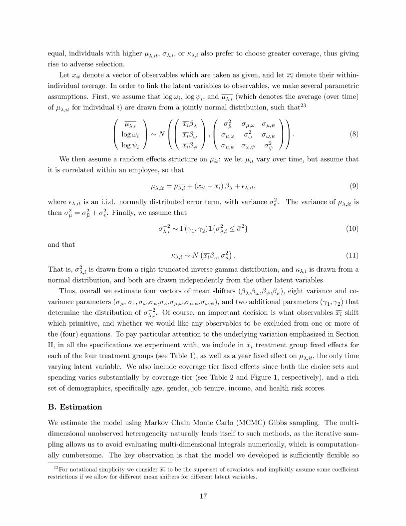
Let xit denote a vector of observables which are taken as given, and let xi denote their within-

individual average. In order to link the latent variables to observables, we make several parametric

assumptions. First, we assume that log!i, log i, and ��;i (which denotes the average (over time)

of ��;it for individual i) are drawn from a jointly normal distribution, such that230B@ ��;i

log!i

log i

1CA � N

0B@0B@ xi��

xi�!

xi�

1CA ;

0B@ �2�� ��;! ��;

��;! �2! �!;

��; �!; �2

1CA1CA : (8)

We then assume a random e¤ects structure on �it: we let �it vary over time, but assume that

it is correlated within an employee, so that

��;it = ��;i + (xit � xi)�� + ��;it; (9)

where ��;it is an i.i.d. normally distributed error term, with variance �2� . The variance of ��;it is

then �2� = �2�� + �2� . Finally, we assume that

��2�;i � �( 1; 2)1f�2�;i � ��2g (10)

and that

��;i � N�xi��; �

2�

�: (11)

That is, �2�;i is drawn from a right truncated inverse gamma distribution, and ��;i is drawn from a

normal distribution, and both are drawn independently from the other latent variables.

Thus, overall we estimate four vectors of mean shifters (��,�!,� ,��), eight variance and co-

variance parameters (��, �"; �!,� ,��,��;!,��; ,�!; ), and two additional parameters ( 1; 2) that

determine the distribution of ��2�;i . Of course, an important decision is what observables xi shift

which primitive, and whether we would like any observables to be excluded from one or more of

the (four) equations. To pay particular attention to the underlying variation emphasized in Section

II, in all the speci�cations we experiment with, we include in xi treatment group �xed e¤ects for

each of the four treatment groups (see Table 1), as well as a year �xed e¤ect on ��;it, the only time

varying latent variable. We also include coverage tier �xed e¤ects since both the choice sets and

spending varies substantially by coverage tier (see Table 2 and Figure 1, respectively), and a rich

set of demographics, speci�cally age, gender, job tenure, income, and health risk scores.

B. Estimation

We estimate the model using Markov Chain Monte Carlo (MCMC) Gibbs sampling. The multi-

dimensional unobserved heterogeneity naturally lends itself to such methods, as the iterative sam-

pling allows us to avoid evaluating multi-dimensional integrals numerically, which is computation-

ally cumbersome. The key observation is that the model we developed is su¢ ciently �exible so

23For notational simplicity we consider xi to be the super-set of covariates, and implicitly assume some coe¢ cientrestrictions if we allow for di¤erent mean shifters for di¤erent latent variables.

17

that we can augment the latent variables into the model and formulate a hierarchical statistical

model. To see this, let �1 =���; �!; � ; ��;��; �"; �!; � ; ��; ��;!; ��; ; �!; ; 1; 2

be the set

of parameters we are interested in, and let �2 =��it; ��;it; ��;i; ��;i; !i; i

i=N;t=2004i=1;t=2003

be the set of

employee-year latent variables. The model is set up so that, even conditional on �1, we can al-

ways rationalize the observed data �namely, plan choice and medical utilization �by appropriately

�nding a set of latent variables for each individual, �2.

Thus, the iterative procedure is straightforward. We can �rst sample from the distribution of �1conditional on �2. Because, conditional on �2, there is no additional information in the data about

�1, this part of the sampling is simple and quite standard. Then, we can sample from the distribution

of �2 conditional on �1 and the information available in the data. This latter step is of course more

customized toward our speci�c model, but does not introduce any conceptual di¢ culties. The full

sampling procedure, the speci�c prior distributions we impose, and the resultant posteriors are

described in detail in Appendix D. We veri�ed using Monte Carlo simulations that the procedure

works e¤ectively, and is robust to initial values. For our baseline results, the estimation appears to

converge after about 5,000 iterations of the Gibbs sampler, so we drop the �rst 10,000 draws and

use the last 10,000 draws of each parameter to report our results. The results we report are based

on the posterior mean and posterior standard deviation from these 10,000 draws.

One important di¢ culty that our model introduces is related to our decision to not allow for an

additive separable plan-speci�c error term. It is extremely common in applications of discrete choice

(such as ours) to add such error terms, and often to assume that they are distributed i.i.d. across

plans and individuals. Such error terms serve two important roles. First, they allow the researcher

to rationalize any choice observed in the data through a large enough error term. Second, their

independence makes the objective function of any M-estimator smooth, which is computationally

attractive for numerical optimization. In the context of our application, however, we view such

error terms as economically unappealing. The options from which individuals in our sample choose

are �nancially rankable and are identical in their non-�nancial features. This makes one wonder

what such error terms would capture that is outside of our model. The clear ranking of the options

also makes the i.i.d. nature of the error terms not very appealing. Instead, we introduce a fair

amount of heterogeneity along the other dimensions of our model. Some of this heterogeneity (e.g.,

the heterogeneity in ��;i and ��;i) is richer than the minimum required to capture the key economic

forces we would like to capture, but this richness is what allows us to rationalize all observed choices

in the data. This still leads to a model which is not very attractive for numerical optimization,

which is one important reason why we use Gibbs sampling.24

C. Identi�cation

We now discuss the identi�cation of the model. Conditional on the individual-behavior model

described in Section I, the object of interest that we seek to identify is the joint distribution of

24 In addition to our previous work (Cohen and Einav, 2007; Einav, Finkelstein, and Schrimpf, 2010), several otherpapers have estimated a discrete choice model without an i.i.d. error, for similar reasons. These include Keane andMo¢ tt (1998), Berry and Pakes (2007), and Goettler and Clay (2011).

18

F�(�), !, and . We have data on individuals� health insurance options, choices, and medical

spending. Throughout the paper we make the strong assumption that individual beliefs about

their subsequent health status (F�(�)) are correct.25

The model and its identi�cation share many properties with some of our earlier work on insur-

ance (Cohen and Einav, 2007; Einav, Finkelstein, and Schrimpf, 2010). The key novel element is

that we now allow for moral hazard, and heterogeneity in it. The panel structure of the data and

the staggered timing of the introduction of the new options are key in allowing us to identify this

new element. We start our discussion of identi�cation by considering nonparametric identi�cation

of our model with ideal data. We then discuss the ways in which our actual data is di¤erent from

the ideal, thus requiring us to make additional parametric assumptions that aid in identi�cation.

The two features of our data set that are instrumental for identi�cation are the panel structure

of the data and the exogenous change in the health insurance options available to employees. In

the ideal setting, we consider a case in which we observe individuals for a su¢ ciently long period

before and a su¢ ciently long period after the change in coverage. Moreover, we assume that the

choice set from which employees can choose coverage is continuous (for example, one can imagine

a continuous coinsurance rate, and an increasing and di¤erentiable mapping from coinsurance rate

to premium).

In such a setting, our model is non-parametrically identi�ed. To see this, note that such

data provide us with two medical expenditure distributions, Gbeforei (m) and Gafteri (m), for each

individual i. Using the realized utility model (during the second period of the model), these two

distributions allow us to recover for each individual Fi;�(�) and !i. To see this, recall that abstractingfrom the truncation of medical spending at zero, our model implies that medical expenditure mit

is equal to �it + !i(1 � ct). If Fi;�(�) is stable over time,26 one can regress (for each employee iseparately) mit on a dummy variable that is equal to 1 after the change. The estimated coe¢ cient

on the dummy variable would be then an estimate of !i (cafter � cbefore), providing an estimate of!i. The distribution of �it can then be recovered by observing that �it = mit � !i(1 � ct), which

is known.

Conditional on Fi;�(�) and !i, individual i�s choice from a continuous set of options provides a

unique mapping from choices to his coe¢ cient of absolute risk aversion since �conditional on Fi;�(�)and !i �the coe¢ cient of risk aversion is the only unknown primitive that may shift employees�

choices, and it does so monotonically. Thus, using information about Fi;�(�) and !i and individuali�s choice from the continuous option set,27 we can recover i. Since we recovered Fi;�(�), !i, and

25While it is reasonable to question this assumption, absent direct data on beliefs some assumption about beliefsis essential for identi�cation. Otherwise, it is not possible to distinguish beliefs from other preferences that onlya¤ect choices, such as risk aversion (see Einav, Finkelstein, and Schrimpf (2010) for a more detailed discussion of thispoint). While we could instead assume some other (pre-speci�ed) form of biased beliefs, correct beliefs seem like anatural starting point.26 If Fi;�(�) changes over time, one could parameterize, identify, and estimate the autocorrelation structure with a

su¢ ciently long panel (the health risk score variable, which varies over time for a given individual, is quite useful inthis regard). We therefore treat Fi;�(�) as stable over time throughout this section.27This can be done using either the options set before the change or after. In fact, the ideal data leads to over

identi�cation, so could allow us to test for the model�s assumoptions and/or to enrich the model.

19

i for each employee, we can now combine these estimates for our entire sample, and obtain the

joint distributions of F�(�), !, and .Our actual data depart from the ideal data described above in two main ways. First, although

we have a panel structure, we only observe individuals for two periods in the baseline sample (that is

limited to 2003 and 2004). Second, the choice set is highly discrete (including three to �ve options)

rather than continuous. We thus make additional parametric assumptions to aid us in identi�cation.

This implies that our identi�cation in the actual estimation cannot rely anymore on identifying the

individual-speci�c parameters employee-by-employee. Rather, we observe a distribution of medical

expenditures before the change and a distribution for medical expenditure after the change. We then

identify the model by comparing the distribution after to the distribution before, using the untreated

individuals to account for time-varying e¤ects in medical spending, just like in the di¤erence-in-

di¤erence analysis of Section III. Once the distribution of moral hazard, !i, is known, the remaining

identi�cation challenge is very similar to our earlier work mentioned above. In the working paper

version (Einav et al., 2011) we provide a more detailed intuition for these last steps.

V. Results

A. Parameter estimates

Table 7(a) presents the estimated parameters from estimating the model on the baseline sample

of 7,570 employee-years. The top panel presents the estimated coe¢ cients on the mean shifters of

the four latent variables: ��;it and ��;i which a¤ect expected health risk (E(�it)), !i which a¤ects

moral hazard, and i which captures risk aversion. The middle panel report the estimated variance-

covariance matrix and the bottom panel reports the estimates of the rest of the parameters. In

Table 7(b) we report some implied quantities of interest that are derived from the estimates. The

latter may be more easy to interpret, so we focus much of the discussion on them.

Overall, as shown in the top panel of Table 7(b), the estimates imply an average health risk

(E(�)) of about $4,340 per employee-year. We estimate an average moral hazard parameter (!)

that is about 30% of the average health risk, or about $1,330 dollar; by way of context, recall that

! is approximately the size of the spending e¤ect as we move individuals from no insurance to full

insurance (see equation (3)).28

We estimate statistically signi�cant and economically large heterogeneity in each one of the

components: health, moral hazard, and risk aversion. One way to gauge the magnitude of this

heterogeneity is in the top panel of Table 7(b). Our estimates indicate a standard deviation for

expected health risk (E(�)) of about $5,100, or a coe¢ cient of variation of about 1.2; the standard

deviation of realized health (�) is, not surprisingly, much larger at $25,000 (not shown). Moral

28We estimate an average coe¢ cient of absolute risk aversion of about 0.0019, but caution against trying to comparethis to existing estimates. In our model, realized utility is a function of both health risk and �nancial risk, while inother papers that estimate risk aversion from insurance choices (e.g., Cohen and Einav, 2007; Handel, 2011) realizedutility is only over �nancial risk. Thus, the estimated level of risk aversion is not directly comparable; indeed, onecould add a separable health related component to utility that is a¤ected only by � to change the risk aversionestimates, without altering anything else in the model.

20

hazard (!) is also estimated to be highly heterogenous, with a standard deviation across employees

of about $3,200, or a coe¢ cient of variation that is greater than 2. Finally, we estimate a coe¢ cient

of variation for absolute risk aversion ( ) that is about one.

The unconditional correlations (Table 7(b), middle panel) are all statistically signi�cant, and

their signs seem reasonable. We estimate that the unconditional correlation between moral hazard

(!) and expected health risk (E(�)) is positive and reasonably important (0.24).This likely re�ects

the fact that in our model moral hazard type (!) is measured in absolute (dollar) terms rather than

relative to health, so individuals with higher E(�) (i.e., worse health) have more opportunities to

exercise moral hazard. The correlation between risk aversion and health risk (and moral hazard) is

negative, perhaps re�ecting the fact that individuals who are more risk averse are also those who

take better care of their health. A similar pattern was documented by Finkelstein and McGarry

(2006) in the context of long-term care insurance. Finally, as may be expected, we estimate a strong

correlation in ��;it over time, of 0.5 (not shown), suggesting that much of an individual�s health

risk is persistent over time, for example due to chronic conditions.

The signs of the covariates seem generally sensible. The bottom panel of Table 7(b) summarizes

the e¤ects of covariates on E(�) by combining their separate e¤ects on �� and ��. As could be

expected, the health risk scores are an important predictor of expected health risk E(�), shifting

it by thousands of dollars in the expected direction. We also estimate that female employees and

employees with non-single coverage are associated with worse expected health (higher E(�)). One

should interpret these latter e¤ects cautiously, however, as health risk scores are partialled out and

are highly correlated with these other variables. This may also explain why the residual e¤ect of

income and tenure on expected health appears negligible.

Our estimates also imply (top panel of Table 7(a)) that employees with higher (i.e., worse)

health risk scores are associated with greater moral hazard and lower risk aversion. Again, this

likely re�ects our choice to model moral hazard in absolute terms rather than relative to health.

Conditional on health risk scores, employees with single coverage appear to be associated with

greater moral hazard as well as with greater risk aversion. This may represent di¤erent process of

decision making regarding health coverage and health care utilization when regarding one self vs.

his family members.

B. Model �t

In Table 8 we report the actual and predicted plan choice probabilities. We �t the choices of

employees who are choosing from the original plan options remarkably well. The �t of the choices

from the new options is also reasonable, but not as good as the �t for the original options. This is

likely because there are many fewer employees in the baseline sample who are subject to the new

options. Thus, to the extent that the same model attempts to rationalize the choices from both

the old and new options, it is natural that more weight is given to trying to �t choices from the old

menu, leading to slightly worse �t for those choosing from the new menu.

Figure 2 reports the actual and predicted distributions of medical expenditure. The top panel

21

reports the �t for the individuals facing the old options, and the bottom panel reports the �t for the

individuals facing the new options. Overall, the �t is quite reasonable. For example, the predicted

average spending is within 10% of actual average spending under both the original and new options,

and the medians also �t quite well. We tend to over predict the fraction of individuals who have

no spending under the new options, but this again is likely driven by the relatively small number

of employees who are switched to the new options in our estimation sample.

Finally, we note that if we simulate data based on our parameter estimates and then run the

di¤erence-in-di¤erences analysis we report on in Section IV, we predict about an 8% reduction in

spending associated with moving from the old option set to the new option set. This is broadly

similar to the di¤erence-in-di¤erences estimates we obtained for the actual data (Table 6, columns

(1)-(3)). However, given how imprecise our di¤erence-in-di¤erences estimates are, both in the actual

data and in the simulated data, we caution against making too much of any comparison. The lack

of statistical signi�cance of the di¤erence-in-di¤erences estimate in the simulated data, relative to

the reasonably precise estimates of the model parameters, suggests that a more complete model of

unobservable heterogeneity and endogenous plan choice is important in increasing precision.

C. Moral hazard estimates

The parameter !i captures moral hazard in our model . Recall that, abstracting from the truncation

of spending at zero, employee i would spend �it in year t if he had no insurance, and with full

insurance would spend �it+ !i: Thus, !i can be thought of as the scope for moral hazard. As

discussed, the top panel of Table 7(b) reports that the estimated average of !i is about 1,330

dollars, or about 30% of the estimated health risk (the average of �it).

Table 9 reports an alternative way one could quantify moral hazard. In the top row of the

table, we calculate each employee�s expected decline in medical expenditure as we move him from

the highest to the lowest coverage in the new options. We will feature the move (or choice) between

these two options in all of our subsequent counterfactual exercises. Recall that, as we have modeled

these options, moving from the highest to the lowest coverage primarily entails moving someone

from a plan with no deductible to a plan with a high deductible, speci�cally a $3,000 deductible for

non-single coverage, or $1,500 for single coverage (Table 2). We estimate that the average spending

e¤ect from this move is $348. The second row reports a similar exercise, but considers moving

individuals from full insurance to no insurance. We estimate an average spending reduction of

$1,273; this is slightly lower than the average !i of $1,330 reported earlier (Table 7(b)) precisely

because of the truncation of spending at zero.

These economically meaningful estimates of moral hazard satisfy one necessary condition for

selection on moral hazard �the focus of our paper �to be important. A second necessary condition

is that moral hazard be heterogeneous. Indeed, we �nd important heterogeneity in our moral

hazard estimates across individuals. For example, the estimated variance of log(!) is about one,

and highly statistically signi�cant (Table 7(a)), implying that an employee who is one standard

deviation above the mean is associated with a moral hazard parameter that is almost three times

22

greater than the mean, and an employee who is one standard deviation below the mean has a moral

hazard parameter that is less than a half of the mean. As shown in the top of Table 7(b), across

individuals, the standard deviation of !i is almost $3,200, and the coe¢ cient of variation of ! is

more than 2.

Again, Table 9 reports more economics-motivated measures of heterogeneity in moral hazard.

The top row shows that the spending decline as we move individuals from the no deductible plan

to the high deductible plan has a standard deviation of $749, compared to the mean of $348. The

median spending reduction is only $48, while the 90th percentile exhibits a spending reduction of

more than a thousand dollars. Similarly, as we move individuals from full insurance to no insurance,

we estimate that the median reduction in spending is $310, but the 90th percentile of the spending

reduction distribution is greater than $3,000.29

D. Selection on moral hazard

The fact that individuals are heterogeneous in their moral hazard response to coverage does not of

course mean that they select on it in any quantitatively meaningful way. That is, it is conceivable

that heterogeneity in other factors is more important in determining plan choice. As one way to

gauge the quantitative importance of selection on moral hazard, we examine how the choice of

coverage varies with the quantiles of the marginal distribution of moral hazard !, and compare this

to how the choice of coverage varies with the quantiles of the marginal distribution of risk aversion

, and of expected health risk E(�). Once again, we focus on the choice between the highest

coverage and lowest coverage plan in the new options (see Table 2). Loosely, our exercise resembles

the introduction of a high deductible health insurance plan into a setting where previously there

was only a no deductible plan. We set the premiums so that, on average, 10% of our sample chooses

the high deductible plan.

Figure 3 reports the results. It shows the fraction of individuals choosing the high deductible

coverage, conditional on the individual being in each quantile of the marginal distribution of moral

hazard !, of risk aversion , and of expected health risk E(�): We present two di¤erent sets

of results. The top panel presents the pattern while taking as given the underlying correlation

structure among these objects. This panel can be thought of as giving the empirical answer to the

question of how much selection there is, on net, on each of the latent primitives that we model.

Given the �exible correlations we allow for, these patterns are a-priori of ambiguous sign. The

bottom panel repeats the same exercise but �shuts down�the e¤ect of the correlation structure. To

do so, we compute the marginal distributions (unconditional on observables) of each of the three

latent variables that a¤ect plan choice (!, , and E(�)), and draw values for the other two latent

variables independently of the value of the variable for which the graph is drawn. This panel can be

thought of as giving the answer to the conceptual comparative static exercise of how much selection

29We explored whether our modeling of moral hazard as an additive shifter of spending is importnat in driving ourestimates of signi�cant heterogeneous moral hazard. Appendix E shows results from an alternative model in whichmoral hazard is modeled as multiplicative rather than additive; we continue to �nd substantial heterogeneity in moralhazard in this alternative model.

23

there is on one latent factor, holding the other factors constant. As discussed previously, demand

for higher coverage generally increases in expected health risk, in risk aversion, and in moral hazard.

Our purpose here is to assess the relative magnitudes. Taken together, the two panels help inform

not only whether empirically there is selection on moral hazard and of what sign (top panel) but

also the extent to which any such selection is primarily �direct� selection based on moral hazard

rather than �indirect� selection arising from the correlation structure between moral hazard and

other factors which may be driving plan choice.

The results in the top panel indicate that empirically there is selection on moral hazard of the

expected sign, with higher moral hazard types (higher !) less likely to choose the high deductible

plan. In terms of the substantive importance of this selection, both panels reveal a similar qualita-

tive pattern: selection on moral hazard is substantially larger than selection on risk aversion and

of similar magnitude to selection on health risk. For example, the top panel indicates that moving

from the 10th percentile to the 90th percentile of the moral hazard distribution is associated with

about a 23 percentage point decline in the demand for the high deductible plan, while moving from

the 10th to the 90th percentile of the expected health risk distribution is associated with about

a 24 percentage point decline in the demand for the high deductible plan. While some of this

re�ects the underlying correlation structure, the �pure� comparative static shown in the bottom

panel produces quite comparable magnitudes. This suggests that much of this selection on moral

hazard is �direct� selection. In other words, in making plan choices, individuals select not only

based on their expected level of spending that they would incur with no insurance, but also on

their expected slope, or incremental spending due to insurance.

By contrast, we �nd selection on risk aversion considerably less important than selection on

either moral hazard or expected health. In our data (see Figure 3(a)) there is very little variation

in demand for the high deductible plan across the centiles of the risk aversion distribution (re�ecting

various correlations), and even the �pure�comparative static (Figure 3(b)) suggests only about a

15 percentage point range between the 10th and 90th percentile.

E. Implications for spending

We investigate the implications of the selection on moral hazard that we detect for attempts to

combat moral hazard through higher consumer cost sharing. To this end, we perform counterfactual

analyses of the spending reduction associated with introducing a lower coverage option. Given our

�nding that higher �moral hazard types�prefer greater coverage, accounting for this selection on

moral hazard suggests that introducing plans with greater consumer cost sharing will produce less

of a spending reduction than would be estimated if selection on moral hazard were ignored, and

it were assumed that those who select the lower coverage option are drawn at random from the

�moral hazard type�distribution.

In the health care sector, the impact of consumer cost sharing on moral hazard is an issue of

considerable policy as well as academic interest. The size and rapid growth of the health care

sector, and the pressure this places on public sector budgets, has created great interest among both

24

academics and policymakers in possible approaches to reducing health care spending. Encouraging

individuals to enroll in plans with higher consumer cost sharing, such as the tax-advantaged Health

Savings Accounts (HSAs) designed to increase enrollment in high deductible plans, is seen as one

potentially promising approach to reducing health spending.

To examine the implications of selection on moral hazard for analysis of such e¤orts, Figure 4

engages in the same exercise as in Figure 3 of giving employees in our sample a choice between the

no deductible and high deductible health insurance plans in the new options. In Figure 3 we �xed

the price of each option and reported the fraction of each quantile of a latent variable who choose

each plan. In Figure 4 we instead gradually increase the (relative) price of the higher coverage

(no deductible) option, and ask how selected is the group of employees who endogenously select

the lower coverage (high deductible) option at each given price. To show the extent of selection,

the �gure reports the average per employee decline in annual spending for those employees who

endogenously select the high deductible plan at each price.

The �gure illustrates strong selection on moral hazard, especially when the share of the high

deductible plan is small. For example, when the price of the no deductible coverage is low enough

so that only 10% of the employees select the high deductible coverage, the average (per employee)

spending decline for those who select the high deductible plan instead of the no deductible plan

is just over $130. By contrast, were all employees to choose the high deductible plan instead of

the no deductible plan, we estimate the per employee spending decline would be about $350. As

noted in the introduction, the common practice in the literature on health insurance and moral

hazard is to look for experimental variation that randomly moves individuals across plans. Such

variation would recover the unconditional average e¤ect of coverage (which is $348 in our context);

this does not account for selection on moral hazard and will therefore substantially over-estimate

the spending reduction associated with the introduction of the high deductible plan when only a

small share of individuals select it.

This selection re�ects the earlier observation that, all else equal, individuals that are associated

with higher moral hazard (higher !i) have higher willingness to pay for insurance, and are therefore

the ones that would be the last to switch to the lowest coverage, as we gradually increase the price

of highest coverage. It is somewhat interesting that in our setting the selection on moral hazard

becomes less important (i.e., the slope of the line in Figure 4 becomes less steep) at higher levels

of prices for the no deductible plans (which leads to greater fractions choosing the high deductible

plan). The same underlying forces are still in play, but are o¤set by the correlation structure with

other primitives.

VI. Illustrative Welfare Analysis

Our �ndings of selection on moral hazard also have implications for policies aimed at reducing selec-

tion. Analysis of how to mitigate selection often focuses on risk adjustment �whereby individual�s

insurance premiums are adjusted on the basis of individual covariates (such as age, gender, and

prior health conditions) that are predictive of expected medical spending. From this perspective,

25

the potential for selection on moral hazard suggests that investments in better monitoring technolo-

gies �such as coinsurance rates that vary across diagnoses (e.g., heart attack vs. headache) or types

of healthcare (e.g., doctor visits vs. inpatient services) with di¤erent behavioral responsiveness to

insurance �may also be e¤ective at ameliorating adverse selection. Our �nal set of counterfactual

analyses considers these issues of contract design by using our model to go further out of sample

and analyze the impact of alternative contract designs on social welfare.30

A. Measuring welfare

Our standard measure of consumer welfare will be the notion of certainty equivalent. That is, for

an individual de�ned by (F�(�); !; ), we denote the certainty equivalent to a contract j by thescalar ej that solves � exp(� ej) = vj(F�(�); !; ), or

ej(F�(�); !; ) � �1

ln

�Zexp(� u�(�; !; j))dF�(�)

�: (12)

Our assumption of CARA utility over (additively separable) income and health implies no income

e¤ects. Because y and pj are taken as given (at the time of utilization choice), it will be convenient

to de�ne eu(m;�; !; j) = �(m� �)� 1

2!(m� �)2

�� cj(m); (13)

so that (based on equation 1) u(m;�; !; j) = eu(m;�; !; j) + y � pj . It will also be convenient to

denote eu�(�; !; j) � eu(m�(�; !; j);�; !; j).

To see the implications of no income e¤ects, we can substitute u�(�; !; j) = eu�(�; !; j) + y� pjinto equation (12) and reorganize to obtain

ej(F�(�); !; ) � eej(F�(�); !; ) + y � pj � � 1 ln

�Zexp(� eu�(�; !; j))dF�(�)�+ y � pj ; (14)

so that eej(F�(�); !; ) captures the welfare from coverage, and residual income enters additively.

Using this notation, di¤erences in ee(�) across contracts with di¤erent coverages capture the will-ingness to pay for coverage. For example, an individual de�ned by (F�(�); !; ) is willing to pay atmost eek(F�(�); !; )� eej(F�(�); !; ) in order to increase his coverage from j to k.

We assume that insurance providers are risk neutral, so that the provider�s welfare is given by

his expected pro�ts, or

�j(F�(�); !) � pj �Z[m�(�; !; j)� cj (m�(�; !; j))] dF�(�); (15)

30Our framework assumes that any moral-hazard induced expenditure represents pure waste from a societal per-spective. While this seems (to us) a natural benchmark �and is in line with the traditional view of moral hazardas a distortion that arises from misaligned incentives that result from the fundamental (risk smoothing) propertiesof providing insurance (e.g., Holmstrom, 1979) � it is reasonable to question whether this literal interpretation isappropriate as a normative statement in the context of health insurance. For example, in the absence of subsidies,liquidity constrained, ill informed, or myopic consumers may under-consume medical care. Absent any clear guidanceas to the nature and magnitude of any such frictions, we abstract from them in our model and note that it is notnecessary to interpret these welfare results in a normative light. It is still a useful metric by which we can quantifyand compare the e¤ects of moral hazard, adverse selection, and di¤erent contract design features.

26

where the integrand captures the share of the utilization covered by the provider under contract j.

Total surplus sj is then given by

sj(F�(�); !; ) = ej(F�(�); !; )+�j(F�(�); !) = eej(F�(�); !; )+y�Z [m�(�; !; j)� cj (m�(�; !; j))] dF�(�):

(16)

That is, total surplus is simply certainty equivalent minus expected cost.

To gain intuition, it may be useful to discuss the nature of the e¢ cient contract in this setting.

Because of our CARA assumption, premiums are a transfer which do not a¤ect total surplus.

Therefore, the e¢ cient contract can be characterized by the e¢ cient coverage function c�(�) thatmaximizes total surplus (as given by equation (16)) over the set of possible coverage functions. Such

optimal contracts would trade o¤ two o¤setting forces. On one hand, an individual is risk averse

while the provider is risk natural, so optimal risk sharing implies full coverage, under which the

individual is not exposed to risk. On the other hand, the presence of moral hazard makes an insured

individual�s privately optimal utilization choice socially ine¢ cient; any positive insurance coverage

makes the individual face a healthcare price which is lower than the social cost of healthcare,

leading to excessive utilization. E¢ cient contracts will therefore resolve this tradeo¤ by some form

of partial coverage (Arrow, 1971; Holmstrom, 1979). For example, it is easy to see that no insurance

(c�(m) = m) is e¢ cient if individuals are risk neutral or face no risk (F�(�) is degenerate), and thatfull insurance (c�(m) = 0) is e¢ cient when moral hazard is not present (! = 0·). In all other

situations, the e¢ cient contract is some form of partial insurance.

B. Welfare implications

Table 10 reports our welfare results. Once again we restrict our attention to a choice between the

no deductible and high deductible plans under the new options (Table 2, options 5 and 1 respec-

tively). Throughout this section we make the simplifying assumption of perfect competition for the

incremental coverage among providers of the no deducible plan, so that the incremental price of the

no deductible plan breaks even for those who provide it: incremental price is equal to incremental

cost.31 We report the implications of various counterfactual contracts for the equilibrium (incre-

mental) premium for the no deductible plan, the share choosing this plan, expected spending per

employee, and total welfare (or surplus) per employee. Our primary focus is on the consequence of

di¤erent contract designs for total welfare (i.e., the sum of consumer welfare and producer welfare)

which in our context is the certainty equivalent minus expected costs (see equation (16)).

The �rst row presents the �status quo�benchmark contract with no (additional) screening or

monitoring. As with the observed contracts in our data, individuals are o¤ered a �uniform�price

that only varies by coverage tier, and insurance companies reimburse medical spending, regardless

of its origin, based on their contract rules. We estimate that the competitive, average incremental

price for the no deductible plan (relative to the high deductible plan) is about $1,570, and that

at this competitive price 90% of the employees would select the no deductible plan. We normalize

31We normalize the price of the lower coverage option to zero. Given our assumptions of CARA utility and arealized utility that is additively separable in income, the price level does not a¤ect plan choice or welfare.

27

total welfare per employee in this status quo benchmark to be zero, so that we can more easily

compare the welfare gains from alternative contract designs.

The second row presents our �perfect screening�counterfactual, which eliminates adverse selec-

tion. Speci�cally, we assume that insurers can observe and price on all the determinants of health

care utilization that the individual knows at the time of his insurance choice �i.e., all of the com-

ponents of F (�) as well as !. We solve for the incremental price of the no deductible plan that

breaks even for each employee individually, thereby eliminating the adverse selection that arises

from uniform pricing. The results indicate that, as expected, the elimination of adverse selection

leads to a lower (average) incremental premium for the no deductible plan, increased coverage (i.e.,

greater fraction choosing the no deductible plan), and higher welfare. It also leads to lower expected

spending since the risk-based pricing disproportionately shifts higher moral hazard (!) individuals

into lower coverage. We estimate the welfare gain per employee from eliminating adverse selection

to be about $52.32

Of particular interest is the contribution of eliminating selection on moral hazard � i.e. one

component of adverse selection �to the total welfare gain from eliminating adverse selection. Row

3 explores this by reporting the welfare gain from eliminating only selection on moral hazard (!)

but continuing to allow selection on health risk (F (�)). Speci�cally, we allow insurers to observe !

and price on it, but not on F (�); thus we are eliminating adverse selection on the slope of health

spending with respect to the insurance contract (!) but not on the level of health spending F (�).

This is of course not a very sensible scenario, since presumably if insurers could observe ! they

could also refuse to reimburse on it, and thus eliminate moral hazard entirely (not just selection on

moral hazard). But it is a conceptually useful way to examine the welfare cost of di¤erent sources

of adverse selection. The results in row 3 suggest that the welfare cost of selection on moral hazard

is $34, or about 65% of the $52 total welfare cost of selection from row 2.

In an analogous fashion, we can investigate the contribution of eliminating selection on moral

hazard to the total welfare gain from eliminating moral hazard. In our setting, the welfare gain from

eliminating moral hazard stems from two sources: removing the allocative ine¢ ciency that arises

from selection on moral hazard and eliminating the traditional moral hazard distortion that comes

through socially ine¢ cient over-utilization of health care. We show the results from eliminating

moral hazard in the fourth row, which presents our �perfect monitoring�counterfactual. Here we

assume that insurance coverage only applies to ��-related�spending, which in the context of our

model means that instead of reimbursing based on actual spending (i.e., reimbursingm�cj(m)), thecontracts reimburse maxf�; 0g � cj(maxf�; 0g) regardless of what the actual spending is. In suchsituations, optimizing individuals would spend maxf�; 0g, which would be the socially e¢ cient levelof spending. Row 4 of Table 10 indicates that, relative to the status quo (row 1), this elimination of

moral hazard reduces spending by more than $1,100 per employee (column 3) and increases welfare

32By way of perspective, we calculate the total surplus from perfect screening relative to everyone being in the highdeductible plan to be $1,084, so that mispricing due to adverse selection appears to reduce welfare by only a smallamount relative to the total surplus at stake. Although not the focus of our paper, this �nding is consistent withother recent empirical papers on the welfare costs arising from ine¢ cient pricing due to adverse selection; see Einav,Finkelstein, and Levin (2010) for a discussion of some of this recent literature.

28

by about $490 per employee, which is an order of magnitude greater relative to the welfare gain

associated with eliminating adverse selection through perfect screening (row 2).

To examine the relative contribution of selection on moral hazard to this welfare cost, in row 5

we again consider an arti�cial counterfactual. Speci�cally, we assume that individuals make their

contract choices in the �rst period as if they are faced with the �perfect monitoring�contracts (row

4), but then in the second period make their spending decision faced with the observed contracts

that reimburse in the same manner as the actual contracts (i.e., reimburse based on m rather than

based on �). This allows us to isolate the welfare gain from eliminating solely selection on moral

hazard, while preserving the distortion in second period consumption caused by moral hazard. The

results suggest that eliminating selection on moral hazard can achieve welfare gains of $25 per

employee, or only about 5% of the total welfare cost of moral hazard (row 4).

Overall, these results suggest that, in our setting, selection on moral hazard contributes non-

trivially to the total welfare cost of selection, but contributes much less relative to the total welfare

cost of moral hazard. At a broad level, our �ndings suggest that in thinking about contract

design, traditional approaches to combatting moral hazard may well aid in combatting selection,

and possibly vice versa. Of course, our quantitative estimates undoubtedly depend on our speci�c

setting (contracts and population) and on our modeling assumptions. While there is not much we

can do about the former (at least in the current paper), we investigate the latter in Appendix F.

VII. Conclusions

This paper takes a �rst step toward marrying empirical analysis of selection with that of moral

hazard. The active (and growing) empirical literature on insurance demand has focused almost

exclusively on selection on the level of risk and on risk preferences, and largely abstracted from moral

hazard.33 The large and venerable literature on moral hazard in insurance has largely focused on

average moral hazard e¤ects, abstracting from potential heterogeneity as well as potential selection

on that heterogeneity. This paper attempts to �ll this gap by introducing the possibility that

individuals�anticipated behavioral response to insurance a¤ects their contract choice. We suggest

that this component of adverse selection can have interesting implications for standard analyses of

both selection and moral hazard.

We explored the existence, nature, and implications of selection on moral hazard empirically in

the context of employer-provided health insurance in the United States. We estimate substantial

heterogeneity in moral hazard and selection on it in our setting, with individuals who have a greater

behavioral response to the contract demanding more coverage. We estimate that heterogeneity in

moral hazard is roughly as important as heterogeneity in expected health risk in determining

whether to buy a higher or lower deductible. In other words, adverse selection based on the

slope of spending (i.e., the incremental spending due to insurance) appears about as quantitatively

important in our setting as adverse selection based on the expected level of spending. We illustrate

some potential implications of such selection on moral hazard. For example, we estimate that

33See Einav, Finkelstein, and Levin (2010) for a recent discussion of this literature.

29

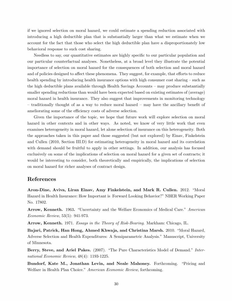
if we ignored selection on moral hazard, we could estimate a spending reduction associated with

introducing a high deductible plan that is substantially larger than what we estimate when we

account for the fact that those who select the high deductible plan have a disproportionately low

behavioral response to such cost sharing.

Needless to say, our quantitative estimates are highly speci�c to our particular population and

our particular counterfactual analyses. Nonetheless, at a broad level they illustrate the potential

importance of selection on moral hazard for the consequences of both selection and moral hazard

and of policies designed to a¤ect these phenomena. They suggest, for example, that e¤orts to reduce

health spending by introducing health insurance options with high consumer cost sharing �such as

the high deductible plans available through Health Savings Accounts �may produce substantially

smaller spending reductions than would have been expected based on existing estimates of (average)

moral hazard in health insurance. They also suggest that improvements in monitoring technology

� traditionally thought of as a way to reduce moral hazard �may have the ancillary bene�t of

ameliorating some of the e¢ ciency costs of adverse selection.

Given the importance of the topic, we hope that future work will explore selection on moral

hazard in other contexts and in other ways. As noted, we know of very little work that even

examines heterogeneity in moral hazard, let alone selection of insurance on this heterogeneity. Both

the approaches taken in this paper and those suggested (but not explored) by Einav, Finkelstein

and Cullen (2010, Section III.D) for estimating heterogeneity in moral hazard and its correlation

with demand should be fruitful to apply in other settings. In addition, our analysis has focused

exclusively on some of the implications of selection on moral hazard for a given set of contracts; it

would be interesting to consider, both theoretically and empirically, the implications of selection

on moral hazard for richer analyses of contract design.

References

Aron-Dine, Aviva, Liran Einav, Amy Finkelstein, and Mark R. Cullen. 2012. �MoralHazard in Health Insurance: How Important is Forward Looking Behavior?�NBERWorking Paper

No. 17802.

Arrow, Kenneth. 1963. �Uncertainty and the Welfare Economics of Medical Care.�AmericanEconomic Review, 53(5): 941-973.

Arrow, Kenneth. 1971. Essays in the Theory of Risk-Bearing. Markham: Chicago, IL.

Bajari, Patrick, Han Hong, Ahmed Khwaja, and Christina Marsh. 2010. �Moral Hazard,Adverse Selection and Health Expenditures: A Semiparametric Analysis.�Manuscript, University

of Minnesota.

Berry, Steve, and Ariel Pakes. (2007). �The Pure Characteristics Model of Demand.� Inter-national Economic Review, 48(4): 1193-1225.

Bundorf, Kate M., Jonathan Levin, and Neale Mahoney. Forthcoming. �Pricing and

Welfare in Health Plan Choice.�American Economic Review, forthcoming.

30

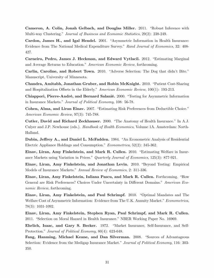
Cameron, A. Colin, Jonah Gelbach, and Douglas Miller. 2011. �Robust Inference withMulti-way Clustering.�Journal of Business and Economic Statistics, 29(2): 238-249.

Cardon, James H., and Igal Hendel. 2001. �Asymmetric Information in Health Insurance:Evidence from The National Medical Expenditure Survey.�Rand Journal of Economics, 32: 408-

427.

Carneiro, Pedro, James J. Heckman, and Edward Vytlacil. 2012. �Estimating Marginaland Average Returns to Education.�American Economic Review, forthcoming.

Carlin, Caroline, and Robert Town. 2010. �Adverse Selection: The Dog that didn�t Bite.�Manuscript, University of Minnesota.

Chandra, Amitabh, Jonathan Gruber, and Robin McKnight. 2010. �Patient Cost-Sharingand Hospitalization O¤sets in the Elderly.�American Economic Review, 100(1): 193-213.

Chiappori, Pierre-André, and Bernard Salanié. 2000. �Testing for Asymmetric Informationin Insurance Markets.�Journal of Political Economy, 108: 56-78.

Cohen, Alma, and Liran Einav. 2007. �Estimating Risk Preferences from Deductible Choice.�

American Economic Review, 97(3): 745-788.

Cutler, David and Richard Zeckhauser. 2000. �The Anatomy of Health Insurance.�In A.J.Culyer and J.P. Newhouse (eds.). Handbook of Health Economics, Volume 1A. Amsterdam: North-

Halland.

Dubin, Je¤rey A., and Daniel L. McFadden. 1984. �An Econometric Analysis of ResidentialElectric Appliance Holdings and Consumption.�Econometrica, 52(2): 345-362.

Einav, Liran, Amy Finkelstein, and Mark R. Cullen. 2010. �Estimating Welfare in Insur-ance Markets using Variation in Prices.�Quarterly Journal of Economics, 125(3): 877-921.

Einav, Liran, Amy Finkelstein, and Jonathan Levin. 2010. �Beyond Testing: EmpiricalModels of Insurance Markets.�Annual Review of Economics, 2: 311-336.

Einav, Liran, Amy Finkelstein, Iuliana Pascu, and Mark R. Cullen. Forthcoming. �HowGeneral are Risk Preferences? Choices Under Uncertainty in Di¤erent Domains.�American Eco-

nomic Review, forthcoming.

Einav, Liran, Amy Finkelstein, and Paul Schrimpf. 2010. �Optimal Mandates and TheWelfare Cost of Asymmetric Information: Evidence from The U.K. Annuity Market.�Econometrica,

78(3): 1031-1092.

Einav, Liran, Amy Finkelstein, Stephen Ryan, Paul Schrimpf, and Mark R. Cullen.2011. �Selection on Moral Hazard in Health Insurance.�NBER Working Paper No. 16969.

Ehrlich, Isaac, and Gary S. Becker. 1972. �Market Insurance, Self-Insurance, and Self-

Protection.�Journal of Political Economy, 80(4): 623-648.

Fang, Hanming, Michael Keane, and Dan Silverman. 2008. �Sources of AdvantageousSelection: Evidence from the Medigap Insurance Market.�Journal of Political Economy, 116: 303-

350.

31

Finkelstein, Amy, and Kathleen McGarry. 2006. �Multiple Dimensions of Private Informa-tion: Evidence from the Long-Term Care Insurance Market.�American Economic Review, 96(4):

938-958.

Gilks, W. R., N.G. Best, and K.K.C. Tan. 1995. �Adaptive Rejection Metropolis Sampling.�Applied Statistics, 44: 455-472.

Goettler, Ronald L., and Karen Clay. 2011. �Tari¤ Choice with Consumer Learning andSwitching Costs.�Journal of Marketing Research, 48(4): 633-652.

Handel, Benjamin. 2011. �Adverse Selection and Switching Costs in Health Insurance Markets:When Nudging Hurts.�Manuscript, UC Berkeley.

Heckman, James J., Sergio Urzua, and Edward Vytlacil. 2006. �Understanding Instru-mental Variables in Models with Essential Heterogeneity.�Review of Economics and Statistics, 88:

389-432.

Holmstrom, Bengt. 1979. �Moral Hazard and Observability.�Bell Journal of Economics, 10(1):74-91.

Keane, Michael, and Robert Mo¢ tt. 1998. �A Structural Model of Multiple Welfare ProgramParticipation and Labor Supply.�International Economic Review, 39(3): 553-589.

Keeler, Emmett B., and John E. Rolph. 1988. �The Demand for Episodes of Treatment inthe Health Insurance Experiment.�Journal of Health Economics, 7: 337-367.

Kowalski, Amanda E. 2010. �Censored Quantile Instrumental Variable Estimates of the PriceElasticity of Expenditure on Medical Care.�NBER Working Paper No. 15085.

Manning, Willard, Joseph Newhouse, Naihua Duan, Emmett Keeler, Arleen Lei-bowitz, and Susan Marquis. 1987. �Health Insurance and the Demand for Medical Care:

Evidence from a Randomized Experiment.�American Economic Review, 77(3): 251-277.

Miravete, Eugenio J. 2003. �Choosing the Wrong Calling Plan? Ignorance and Learning.�

American Economic Review, 93(1): 297-310.

Newhouse, Joseph. 1993. Free for All? Lessons from the RAND Health Insurance Experiment.

Harvard University Press: Cambridge, MA.

Pauly, Mark. 1968. �The Economics of Moral Hazard: Comment.�American Economic Review,58(3): 531-537.

Wooldridge, Je¤rey M. (2002). Econometric Analysis of Cross Section and Panel Data. MITPress: Cambridge, MA.

32

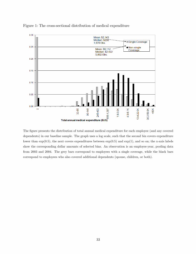
Figure 1: The cross-sectional distribution of medical expenditure

The �gure presents the distribution of total annual medical expenditure for each employee (and any covered

dependents) in our baseline sample. The graph uses a log scale, such that the second bin covers expenditure

lower than exp(0.5), the next covers expenditures between exp(0.5) and exp(1), and so on; the x-axis labels

show the corresponding dollar amounts of selected bins. An observation is an employee-year, pooling data

from 2003 and 2004. The grey bars correspond to employees with a single coverage, while the black bars

correspond to employees who also covered additional dependents (spouse, children, or both).

33

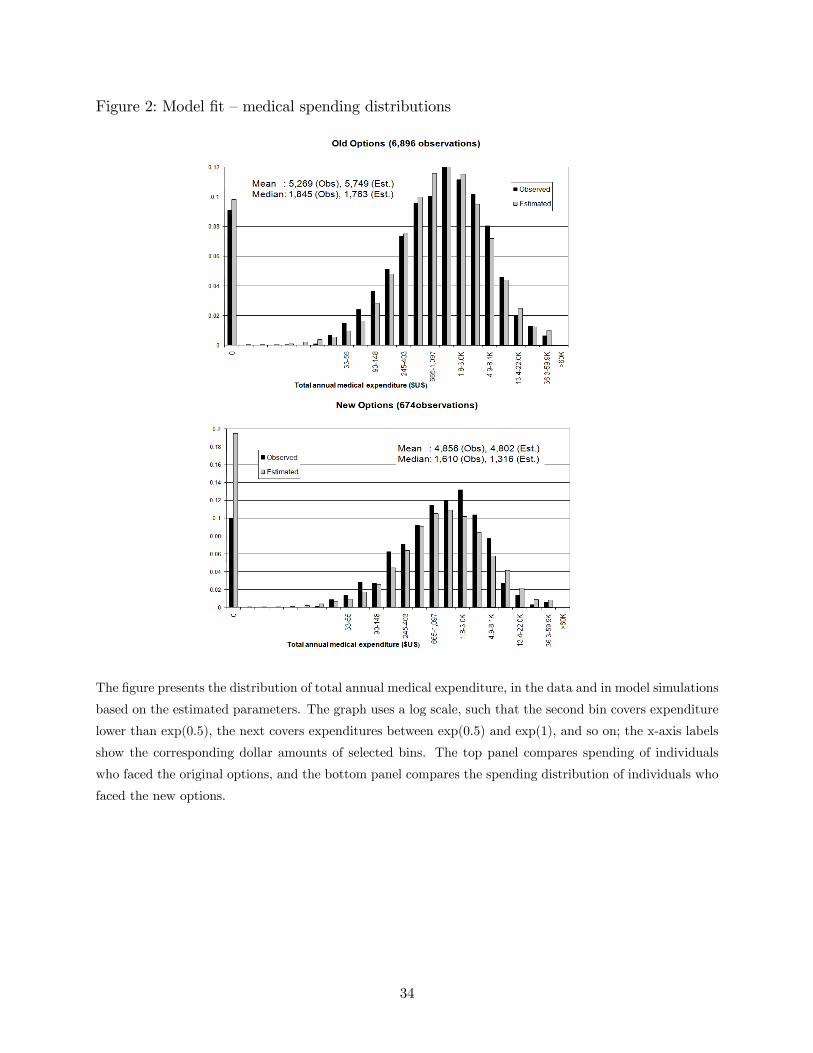
Figure 2: Model �t �medical spending distributions

The �gure presents the distribution of total annual medical expenditure, in the data and in model simulations

based on the estimated parameters. The graph uses a log scale, such that the second bin covers expenditure

lower than exp(0.5), the next covers expenditures between exp(0.5) and exp(1), and so on; the x-axis labels

show the corresponding dollar amounts of selected bins. The top panel compares spending of individuals

who faced the original options, and the bottom panel compares the spending distribution of individuals who

faced the new options.

34

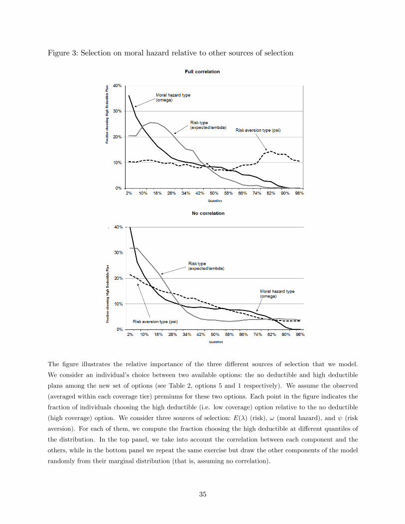
Figure 3: Selection on moral hazard relative to other sources of selection

The �gure illustrates the relative importance of the three di¤erent sources of selection that we model.

We consider an individual�s choice between two available options: the no deductible and high deductible

plans among the new set of options (see Table 2, options 5 and 1 respectively). We assume the observed

(averaged within each coverage tier) premiums for these two options. Each point in the �gure indicates the

fraction of individuals choosing the high deductible (i.e. low coverage) option relative to the no deductible

(high coverage) option. We consider three sources of selection: E(�) (risk), ! (moral hazard), and (risk

aversion). For each of them, we compute the fraction choosing the high deductible at di¤erent quantiles of

the distribution. In the top panel, we take into account the correlation between each component and the

others, while in the bottom panel we repeat the same exercise but draw the other components of the model

randomly from their marginal distribution (that is, assuming no correlation).

35

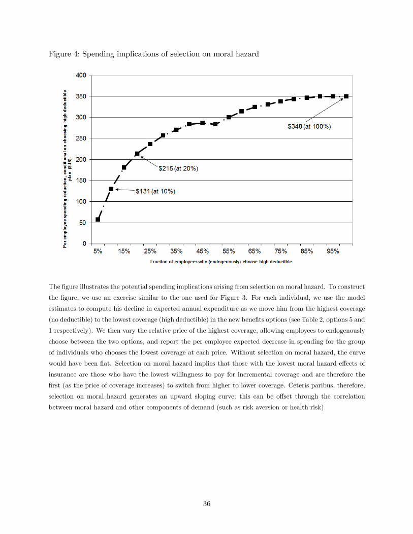
Figure 4: Spending implications of selection on moral hazard

The �gure illustrates the potential spending implications arising from selection on moral hazard. To construct

the �gure, we use an exercise similar to the one used for Figure 3. For each individual, we use the model

estimates to compute his decline in expected annual expenditure as we move him from the highest coverage

(no deductible) to the lowest coverage (high deductible) in the new bene�ts options (see Table 2, options 5 and

1 respectively). We then vary the relative price of the highest coverage, allowing employees to endogenously

choose between the two options, and report the per-employee expected decrease in spending for the group

of individuals who chooses the lowest coverage at each price. Without selection on moral hazard, the curve

would have been �at. Selection on moral hazard implies that those with the lowest moral hazard e¤ects of

insurance are those who have the lowest willingness to pay for incremental coverage and are therefore the

�rst (as the price of coverage increases) to switch from higher to lower coverage. Ceteris paribus, therefore,

selection on moral hazard generates an upward sloping curve; this can be o¤set through the correlation

between moral hazard and other components of demand (such as risk aversion or health risk).

36

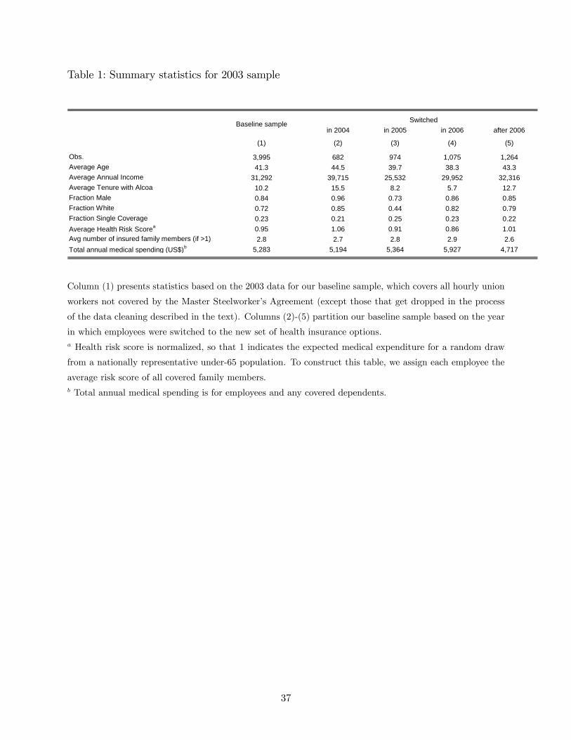
Table 1: Summary statistics for 2003 sample

in 2004 in 2005 in 2006 after 2006

(1) (2) (3) (4) (5)

Obs. 3,995 682 974 1,075 1,264Average Age 41.3 44.5 39.7 38.3 43.3Average Annual Income 31,292 39,715 25,532 29,952 32,316Average Tenure with Alcoa 10.2 15.5 8.2 5.7 12.7Fraction Male 0.84 0.96 0.73 0.86 0.85Fraction White 0.72 0.85 0.44 0.82 0.79Fraction Single Coverage 0.23 0.21 0.25 0.23 0.22Average Health Risk Scorea 0.95 1.06 0.91 0.86 1.01Avg number of insured family members (if >1) 2.8 2.7 2.8 2.9 2.6Total annual medical spending (US$)b 5,283 5,194 5,364 5,927 4,717

SwitchedBaseline sample

Column (1) presents statistics based on the 2003 data for our baseline sample, which covers all hourly union

workers not covered by the Master Steelworker�s Agreement (except those that get dropped in the process

of the data cleaning described in the text). Columns (2)-(5) partition our baseline sample based on the year

in which employees were switched to the new set of health insurance options.a Health risk score is normalized, so that 1 indicates the expected medical expenditure for a random draw

from a nationally representative under-65 population. To construct this table, we assign each employee the

average risk score of all covered family members.b Total annual medical spending is for employees and any covered dependents.

37

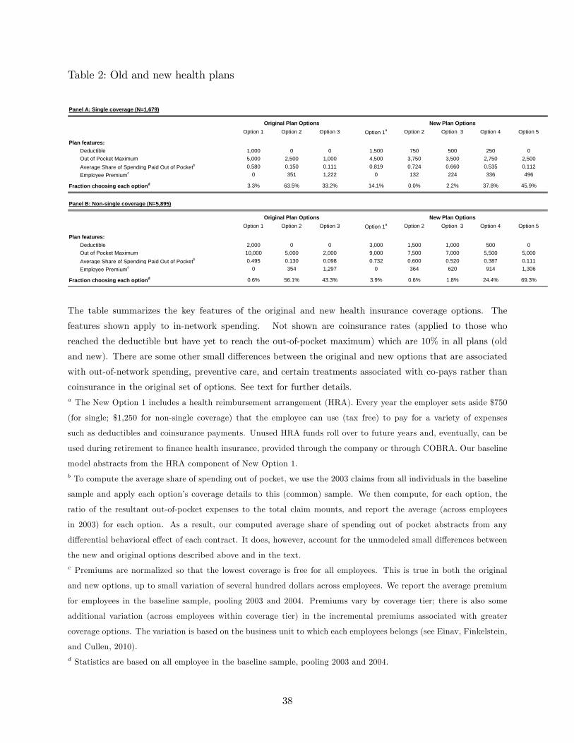
Table 2: Old and new health plans

Panel A: Single coverage (N=1,679)

Option 1 Option 2 Option 3 Option 1a Option 2 Option  3 Option 4 Option 5

Plan features:Deductible 1,000 0 0 1,500 750 500 250 0Out of Pocket Maximum 5,000 2,500 1,000 4,500 3,750 3,500 2,750 2,500Average Share of Spending Paid Out of Pocketb 0.580 0.150 0.111 0.819 0.724 0.660 0.535 0.112Employee Premiumc 0 351 1,222 0 132 224 336 496

Fraction choosing each optiond 3.3% 63.5% 33.2% 14.1% 0.0% 2.2% 37.8% 45.9%

Panel B: Non­single coverage (N=5,895)

Option 1 Option 2 Option 3 Option 1a Option 2 Option  3 Option 4 Option 5

Plan features:Deductible 2,000 0 0 3,000 1,500 1,000 500 0Out of Pocket Maximum 10,000 5,000 2,000 9,000 7,500 7,000 5,500 5,000Average Share of Spending Paid Out of Pocketb 0.495 0.130 0.098 0.732 0.600 0.520 0.387 0.111Employee Premiumc 0 354 1,297 0 364 620 914 1,306

Fraction choosing each optiond 0.6% 56.1% 43.3% 3.9% 0.6% 1.8% 24.4% 69.3%

Original Plan Options New Plan Options

Original Plan Options New Plan Options

The table summarizes the key features of the original and new health insurance coverage options. The

features shown apply to in-network spending. Not shown are coinsurance rates (applied to those who

reached the deductible but have yet to reach the out-of-pocket maximum) which are 10% in all plans (old

and new). There are some other small di¤erences between the original and new options that are associated

with out-of-network spending, preventive care, and certain treatments associated with co-pays rather than

coinsurance in the original set of options. See text for further details.a The New Option 1 includes a health reimbursement arrangement (HRA). Every year the employer sets aside $750

(for single; $1,250 for non-single coverage) that the employee can use (tax free) to pay for a variety of expenses

such as deductibles and coinsurance payments. Unused HRA funds roll over to future years and, eventually, can be

used during retirement to �nance health insurance, provided through the company or through COBRA. Our baseline

model abstracts from the HRA component of New Option 1.b To compute the average share of spending out of pocket, we use the 2003 claims from all individuals in the baseline

sample and apply each option�s coverage details to this (common) sample. We then compute, for each option, the

ratio of the resultant out-of-pocket expenses to the total claim mounts, and report the average (across employees

in 2003) for each option. As a result, our computed average share of spending out of pocket abstracts from any

di¤erential behavioral e¤ect of each contract. It does, however, account for the unmodeled small di¤erences between

the new and original options described above and in the text.c Premiums are normalized so that the lowest coverage is free for all employees. This is true in both the original

and new options, up to small variation of several hundred dollars across employees. We report the average premium

for employees in the baseline sample, pooling 2003 and 2004. Premiums vary by coverage tier; there is also some

additional variation (across employees within coverage tier) in the incremental premiums associated with greater

coverage options. The variation is based on the business unit to which each employees belongs (see Einav, Finkelstein,

and Cullen, 2010).d Statistics are based on all employee in the baseline sample, pooling 2003 and 2004.

38

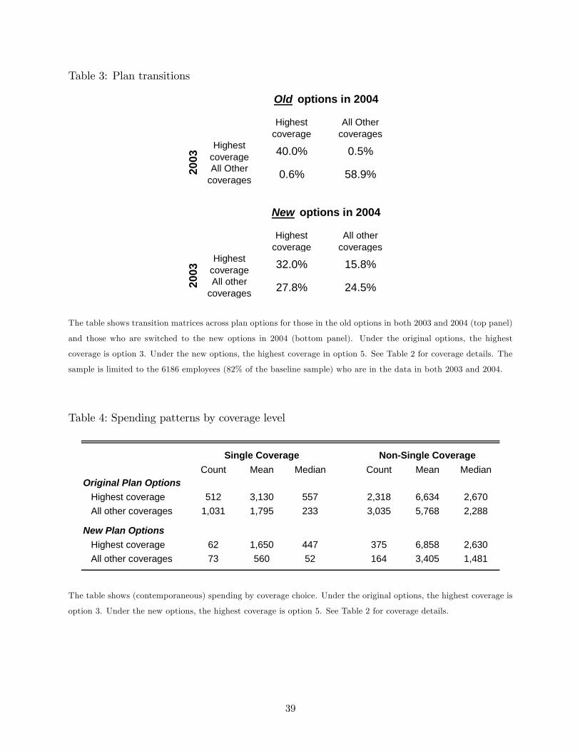
Table 3: Plan transitions

Highestcoverage

All Othercoverages

Highestcoverage 40.0% 0.5%All Other

coverages 0.6% 58.9%

Highestcoverage

All othercoverages

Highestcoverage 32.0% 15.8%All other

coverages 27.8% 24.5%2003

Old  options in 2004

2003

New  options in 2004

The table shows transition matrices across plan options for those in the old options in both 2003 and 2004 (top panel)

and those who are switched to the new options in 2004 (bottom panel). Under the original options, the highest

coverage is option 3. Under the new options, the highest coverage in option 5. See Table 2 for coverage details. The

sample is limited to the 6186 employees (82% of the baseline sample) who are in the data in both 2003 and 2004.

Table 4: Spending patterns by coverage level

Count Mean Median Count Mean MedianOriginal Plan Options   Highest coverage 512 3,130 557 2,318 6,634 2,670   All other coverages 1,031 1,795 233 3,035 5,768 2,288

New Plan Options   Highest coverage 62 1,650 447 375 6,858 2,630   All other coverages 73 560 52 164 3,405 1,481

Single Coverage Non­Single Coverage

The table shows (contemporaneous) spending by coverage choice. Under the original options, the highest coverage is

option 3. Under the new options, the highest coverage is option 5. See Table 2 for coverage details.

39

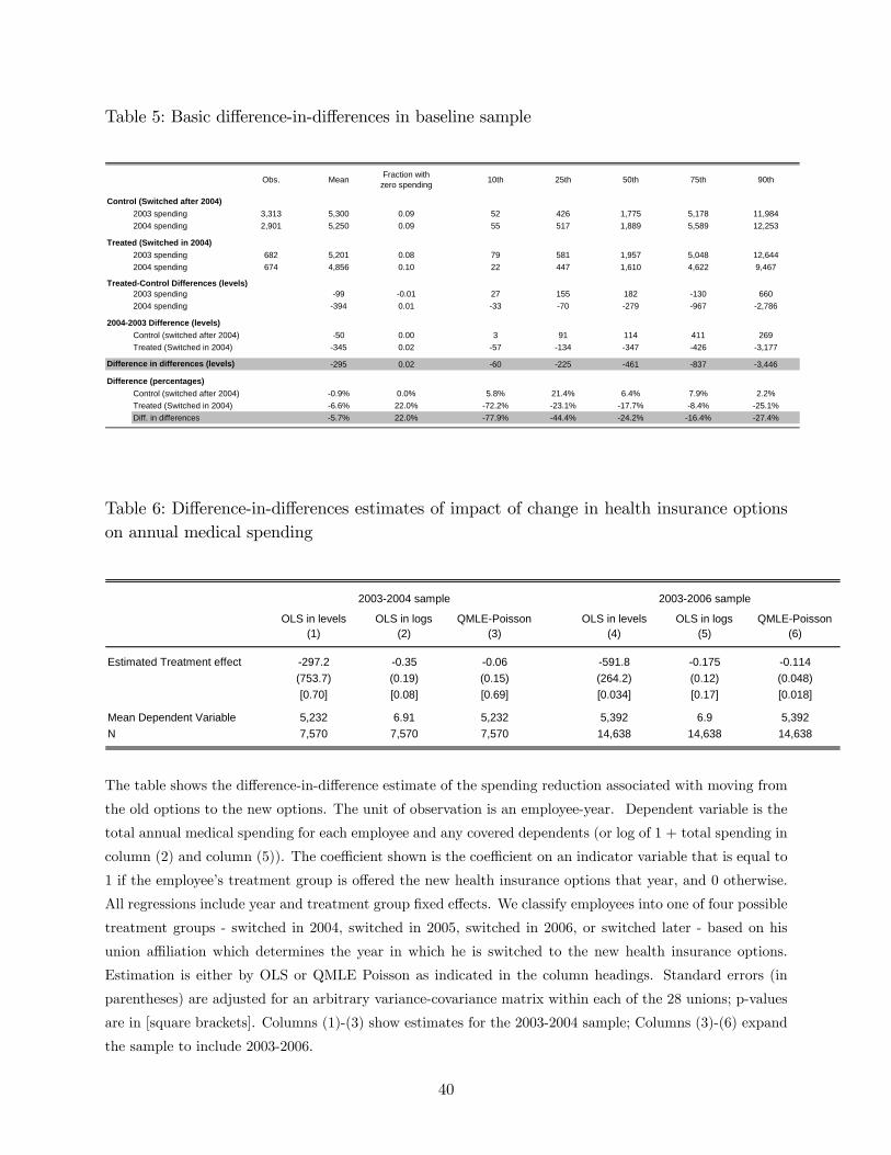
Table 5: Basic di¤erence-in-di¤erences in baseline sample

Obs. Mean Fraction withzero spending 10th 25th 50th 75th 90th

Control (Switched after 2004)2003 spending 3,313 5,300 0.09 52 426 1,775 5,178 11,9842004 spending 2,901 5,250 0.09 55 517 1,889 5,589 12,253

Treated (Switched in 2004)2003 spending 682 5,201 0.08 79 581 1,957 5,048 12,6442004 spending 674 4,856 0.10 22 447 1,610 4,622 9,467

2003 spending ­99 ­0.01 27 155 182 ­130 6602004 spending ­394 0.01 ­33 ­70 ­279 ­967 ­2,786

2004­2003 Difference (levels)Control (switched after 2004) ­50 0.00 3 91 114 411 269Treated (Switched in 2004) ­345 0.02 ­57 ­134 ­347 ­426 ­3,177

­295 0.02 ­60 ­225 ­461 ­837 ­3,446

Difference (percentages)Control (switched after 2004) ­0.9% 0.0% 5.8% 21.4% 6.4% 7.9% 2.2%Treated (Switched in 2004) ­6.6% 22.0% ­72.2% ­23.1% ­17.7% ­8.4% ­25.1%Diff. in differences ­5.7% 22.0% ­77.9% ­44.4% ­24.2% ­16.4% ­27.4%

Treated­Control Differences (levels)

Difference in differences (levels)

Table 6: Di¤erence-in-di¤erences estimates of impact of change in health insurance optionson annual medical spending

OLS in levels OLS in logs QMLE­Poisson OLS in levels OLS in logs QMLE­Poisson(1) (2) (3) (4) (5) (6)

Estimated Treatment effect ­297.2 ­0.35 ­0.06 ­591.8 ­0.175 ­0.114(753.7) (0.19) (0.15) (264.2) (0.12) (0.048)[0.70] [0.08] [0.69] [0.034] [0.17] [0.018]

Mean Dependent Variable 5,232 6.91 5,232 5,392 6.9 5,392N 7,570 7,570 7,570 14,638 14,638 14,638

2003­2004 sample 2003­2006 sample

The table shows the di¤erence-in-di¤erence estimate of the spending reduction associated with moving from

the old options to the new options. The unit of observation is an employee-year. Dependent variable is the

total annual medical spending for each employee and any covered dependents (or log of 1 + total spending in

column (2) and column (5)). The coe¢ cient shown is the coe¢ cient on an indicator variable that is equal to

1 if the employee�s treatment group is o¤ered the new health insurance options that year, and 0 otherwise.

All regressions include year and treatment group �xed e¤ects. We classify employees into one of four possible

treatment groups - switched in 2004, switched in 2005, switched in 2006, or switched later - based on his

union a¢ liation which determines the year in which he is switched to the new health insurance options.

Estimation is either by OLS or QMLE Poisson as indicated in the column headings. Standard errors (in

parentheses) are adjusted for an arbitrary variance-covariance matrix within each of the 28 unions; p-values

are in [square brackets]. Columns (1)-(3) show estimates for the 2003-2004 sample; Columns (3)-(6) expand

the sample to include 2003-2006.

40

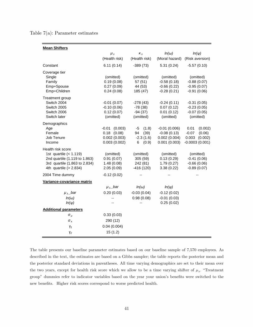
Table 7(a): Parameter estimates

Mean Shiftersμ λ κ λ ln(ω) ln(ψ)

(Health risk) (Health risk) (Moral hazard) (Risk aversion)

Constant 6.11 (0.14) ­389 (73) 5.31 (0.24) ­5.57 (0.10)

Coverage tier   Single (omitted) (omitted) (omitted) (omitted)   Family  0.19 (0.08) 57 (51) ­0.58 (0.18) ­0.88 (0.07)   Emp+Spouse  0.27 (0.09) 44 (53) ­0.66 (0.22) ­0.95 (0.07)   Emp+Children  0.24 (0.08) 185 (47) ­0.28 (0.21) ­0.91 (0.06)

Treatment group   Switch 2004 ­0.01 (0.07) ­278 (43) ­0.24 (0.11) ­0.31 (0.05)   Switch 2005 ­0.10 (0.06) ­78 (38) 0.07 (0.12) ­0.23 (0.05)   Switch 2006  0.12 (0.07) ­94 (37) 0.01 (0.12) ­0.07 (0.05)   Switch later (omitted) (omitted) (omitted) (omitted)

DemographicsAge   ­0.01   (0.003)      ­5    (1.8) ­0.01 (0.006)    0.01    (0.002)Female  0.18   (0.08)    94    (39) ­0.08 (0.13) ­0.07    (0.06)Job Tenure    0.002 (0.003)      ­2.3 (1.6) 0.002 (0.004)  0.003   (0.002)Income    0.003 (0.002)       6    (0.9) 0.001 (0.003) ­0.0003 (0.001)

Health risk score   1st  quartile (< 1.119) (omitted) (omitted) (omitted) (omitted)   2nd quartile (1.119 to 1.863) 0.91 (0.07)   305 (59) 0.13 (0.29) ­0.41 (0.06)   3rd  quartile (1.863 to 2.834) 1.48 (0.08)   242 (81) 1.79 (0.27) ­0.66 (0.06)   4th  quartile (> 2.834) 2.05 (0.09)   ­416 (120) 3.38 (0.22) ­0.89 (0.07)

2004 Time dummy ­0.12 (0.02) ­­ ­­ ­­

Variance­covariance matrixμ λ _bar ln(ω) ln(ψ)

μ λ _bar 0.20 (0.03) ­0.03 (0.04) ­0.12 (0.02)ln(ω) ­­  0.98 (0.08) ­0.01 (0.03)ln(ψ) ­­ ­­  0.25 (0.02)

Additional parametersσ μ 0.33 (0.03)σ κ 290 (12) γ1 0.04 (0.004)γ2 15 (1.2)

The table presents our baseline parameter estimates based on our baseline sample of 7,570 employees. As

described in the text, the estimates are based on a Gibbs sampler; the table reports the posterior mean and

the posterior standard deviations in parentheses. All time varying demographics are set to their mean over

the two years, except for health risk score which we allow to be a time varying shifter of ��: �Treatment

group�dummies refer to indicator variables based on the year your union�s bene�ts were switched to the

new bene�ts. Higher risk scores correspond to worse predicted health.

41

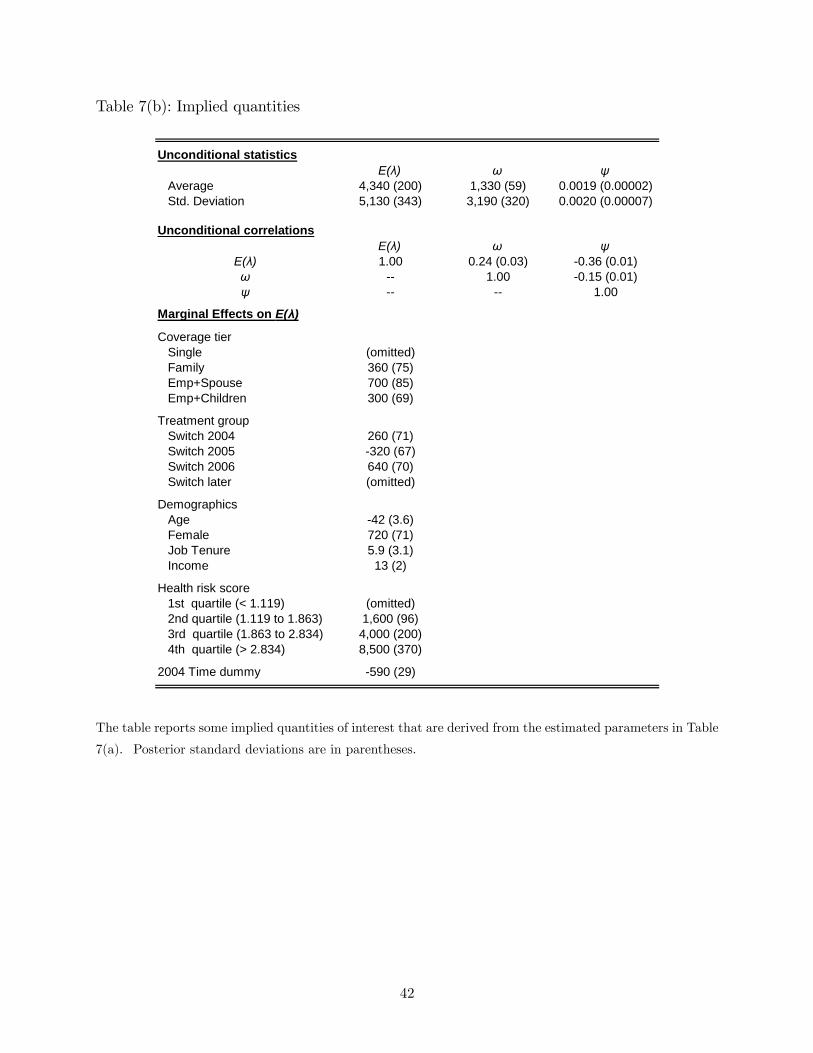
Table 7(b): Implied quantities

Unconditional statisticsE(λ) ω ψ

   Average 4,340 (200) 1,330 (59) 0.0019 (0.00002)   Std. Deviation 5,130 (343) 3,190 (320) 0.0020 (0.00007)

Unconditional correlationsE(λ) ω ψ

E(λ) 1.00 0.24 (0.03) ­0.36 (0.01)ω ­­ 1.00 ­0.15 (0.01)ψ ­­ ­­ 1.00

Marginal Effects on E(λ)

Coverage tier   Single (omitted)   Family 360 (75)   Emp+Spouse 700 (85)   Emp+Children 300 (69)

Treatment group   Switch 2004 260 (71)   Switch 2005 ­320 (67)   Switch 2006 640 (70)   Switch later (omitted)

DemographicsAge ­42 (3.6)Female 720 (71)Job Tenure 5.9 (3.1)Income 13 (2)

Health risk score   1st  quartile (< 1.119) (omitted)   2nd quartile (1.119 to 1.863) 1,600 (96)   3rd  quartile (1.863 to 2.834) 4,000 (200)   4th  quartile (> 2.834) 8,500 (370)

2004 Time dummy ­590 (29)

The table reports some implied quantities of interest that are derived from the estimated parameters in Table

7(a). Posterior standard deviations are in parentheses.

42

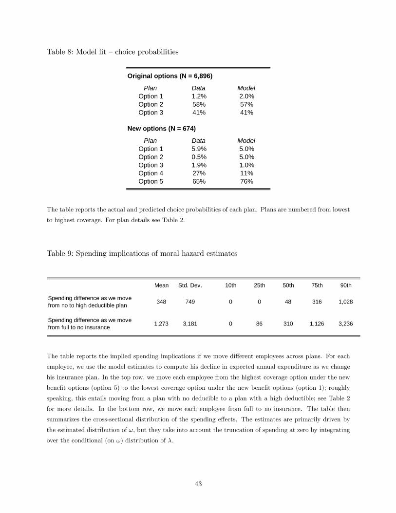
Table 8: Model �t �choice probabilities

Original options (N = 6,896)

Plan Data ModelOption 1 1.2% 2.0%Option 2 58% 57%Option 3 41% 41%

New options (N = 674)

Plan Data ModelOption 1 5.9% 5.0%Option 2 0.5% 5.0%Option 3 1.9% 1.0%Option 4 27% 11%Option 5 65% 76%

The table reports the actual and predicted choice probabilities of each plan. Plans are numbered from lowest

to highest coverage. For plan details see Table 2.

Table 9: Spending implications of moral hazard estimates

Mean Std. Dev. 10th 25th 50th 75th 90th

Spending difference as we movefrom no to high deductible plan 348 749 0 0 48 316 1,028

Spending difference as we movefrom full to no insurance 1,273 3,181 0 86 310 1,126 3,236

The table reports the implied spending implications if we move di¤erent employees across plans. For each

employee, we use the model estimates to compute his decline in expected annual expenditure as we change

his insurance plan. In the top row, we move each employee from the highest coverage option under the new

bene�t options (option 5) to the lowest coverage option under the new bene�t options (option 1); roughly

speaking, this entails moving from a plan with no deducible to a plan with a high deductible; see Table 2

for more details. In the bottom row, we move each employee from full to no insurance. The table then

summarizes the cross-sectional distribution of the spending e¤ects. The estimates are primarily driven by

the estimated distribution of !, but they take into account the truncation of spending at zero by integrating

over the conditional (on !) distribution of �:

43

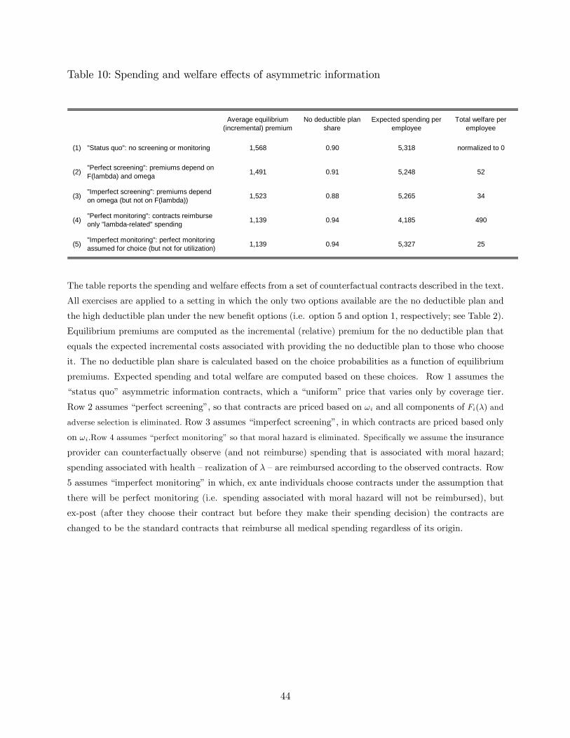
Table 10: Spending and welfare e¤ects of asymmetric information

Average equilibrium(incremental) premium

No deductible planshare

Expected spending peremployee

Total welfare peremployee

(1) "Status quo": no screening or monitoring 1,568 0.90 5,318 normalized to 0

(2) "Perfect screening": premiums depend onF(lambda) and omega 1,491 0.91 5,248 52

(3) "Imperfect screening": premiums dependon omega (but not on F(lambda)) 1,523 0.88 5,265 34

(4) "Perfect monitoring": contracts reimburseonly "lambda­related" spending 1,139 0.94 4,185 490

(5) "Imperfect monitoring": perfect monitoringassumed for choice (but not for utilization) 1,139 0.94 5,327 25

The table reports the spending and welfare e¤ects from a set of counterfactual contracts described in the text.

All exercises are applied to a setting in which the only two options available are the no deductible plan and

the high deductible plan under the new bene�t options (i.e. option 5 and option 1, respectively; see Table 2).

Equilibrium premiums are computed as the incremental (relative) premium for the no deductible plan that

equals the expected incremental costs associated with providing the no deductible plan to those who choose

it. The no deductible plan share is calculated based on the choice probabilities as a function of equilibrium

premiums. Expected spending and total welfare are computed based on these choices. Row 1 assumes the

�status quo�asymmetric information contracts, which a �uniform�price that varies only by coverage tier.

Row 2 assumes �perfect screening�, so that contracts are priced based on !i and all components of Fi(�) and

adverse selection is eliminated. Row 3 assumes �imperfect screening�, in which contracts are priced based only

on !i:Row 4 assumes �perfect monitoring�so that moral hazard is eliminated. Speci�cally we assume the insurance

provider can counterfactually observe (and not reimburse) spending that is associated with moral hazard;

spending associated with health �realization of � �are reimbursed according to the observed contracts. Row

5 assumes �imperfect monitoring�in which, ex ante individuals choose contracts under the assumption that

there will be perfect monitoring (i.e. spending associated with moral hazard will not be reimbursed), but

ex-post (after they choose their contract but before they make their spending decision) the contracts are

changed to be the standard contracts that reimburse all medical spending regardless of its origin.

44

ONLINE APPENDICES.

NOT FOR PUBLICATION.

45

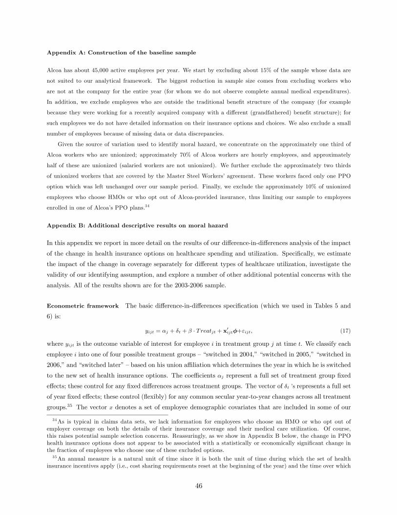
Appendix A: Construction of the baseline sample

Alcoa has about 45,000 active employees per year. We start by excluding about 15% of the sample whose data are

not suited to our analytical framework. The biggest reduction in sample size comes from excluding workers who

are not at the company for the entire year (for whom we do not observe complete annual medical expenditures).

In addition, we exclude employees who are outside the traditional bene�t structure of the company (for example

because they were working for a recently acquired company with a di¤erent (grandfathered) bene�t structure); for

such employees we do not have detailed information on their insurance options and choices. We also exclude a small

number of employees because of missing data or data discrepancies.

Given the source of variation used to identify moral hazard, we concentrate on the approximately one third of

Alcoa workers who are unionized; approximately 70% of Alcoa workers are hourly employees, and approximately

half of these are unionized (salaried workers are not unionized). We further exclude the approximately two thirds

of unionized workers that are covered by the Master Steel Workers�agreement. These workers faced only one PPO

option which was left unchanged over our sample period. Finally, we exclude the approximately 10% of unionized

employees who choose HMOs or who opt out of Alcoa-provided insurance, thus limiting our sample to employees

enrolled in one of Alcoa�s PPO plans.34

Appendix B: Additional descriptive results on moral hazard

In this appendix we report in more detail on the results of our di¤erence-in-di¤erences analysis of the impact

of the change in health insurance options on healthcare spending and utilization. Speci�cally, we estimate

the impact of the change in coverage separately for di¤erent types of healthcare utilization, investigate the

validity of our identifying assumption, and explore a number of other additional potential concerns with the

analysis. All of the results shown are for the 2003-2006 sample.

Econometric framework The basic di¤erence-in-di¤erences speci�cation (which we used in Tables 5 and

6) is:

yijt = �j + �t + � � Treatjt + x0ijt�+"ijt; (17)

where yijt is the outcome variable of interest for employee i in treatment group j at time t. We classify each

employee i into one of four possible treatment groups ��switched in 2004,��switched in 2005,��switched in

2006,�and �switched later��based on his union a¢ liation which determines the year in which he is switched

to the new set of health insurance options. The coe¢ cients �j represent a full set of treatment group �xed

e¤ects; these control for any �xed di¤erences across treatment groups. The vector of �t �s represents a full set

of year �xed e¤ects; these control (�exibly) for any common secular year-to-year changes across all treatment

groups.35 The vector x denotes a set of employee demographic covariates that are included in some of our

34As is typical in claims data sets, we lack information for employees who choose an HMO or who opt out ofemployer coverage on both the details of their insurance coverage and their medical care utilization. Of course,this raises potential sample selection concerns. Reassuringly, as we show in Appendix B below, the change in PPOhealth insurance options does not appear to be associated with a statistically or economically signi�cant change inthe fraction of employees who choose one of these excluded options.35An annual measure is a natural unit of time since it is both the unit of time during which the set of health

insurance incentives apply (i.e., cost sharing requirements reset at the beginning of the year) and the time over which

46

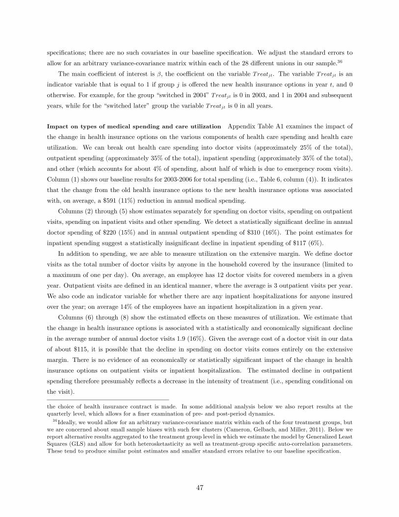
speci�cations; there are no such covariates in our baseline speci�cation. We adjust the standard errors to

allow for an arbitrary variance-covariance matrix within each of the 28 di¤erent unions in our sample.36

The main coe¢ cient of interest is �, the coe¢ cient on the variable Treatjt. The variable Treatjt is an

indicator variable that is equal to 1 if group j is o¤ered the new health insurance options in year t, and 0

otherwise. For example, for the group �switched in 2004�Treatjt is 0 in 2003, and 1 in 2004 and subsequent

years, while for the �switched later�group the variable Treatjt is 0 in all years.

Impact on types of medical spending and care utilization Appendix Table A1 examines the impact of

the change in health insurance options on the various components of health care spending and health care

utilization. We can break out health care spending into doctor visits (approximately 25% of the total),

outpatient spending (approximately 35% of the total), inpatient spending (approximately 35% of the total),

and other (which accounts for about 4% of spending, about half of which is due to emergency room visits).

Column (1) shows our baseline results for 2003-2006 for total spending (i.e., Table 6, column (4)). It indicates

that the change from the old health insurance options to the new health insurance options was associated

with, on average, a $591 (11%) reduction in annual medical spending.

Columns (2) through (5) show estimates separately for spending on doctor visits, spending on outpatient

visits, spending on inpatient visits and other spending. We detect a statistically signi�cant decline in annual

doctor spending of $220 (15%) and in annual outpatient spending of $310 (16%). The point estimates for

inpatient spending suggest a statistically insigni�cant decline in inpatient spending of $117 (6%).

In addition to spending, we are able to measure utilization on the extensive margin. We de�ne doctor

visits as the total number of doctor visits by anyone in the household covered by the insurance (limited to

a maximum of one per day). On average, an employee has 12 doctor visits for covered members in a given

year. Outpatient visits are de�ned in an identical manner, where the average is 3 outpatient visits per year.

We also code an indicator variable for whether there are any inpatient hospitalizations for anyone insured

over the year; on average 14% of the employees have an inpatient hospitalization in a given year.

Columns (6) through (8) show the estimated e¤ects on these measures of utilization. We estimate that

the change in health insurance options is associated with a statistically and economically signi�cant decline

in the average number of annual doctor visits 1.9 (16%). Given the average cost of a doctor visit in our data

of about $115, it is possible that the decline in spending on doctor visits comes entirely on the extensive

margin. There is no evidence of an economically or statistically signi�cant impact of the change in health

insurance options on outpatient visits or inpatient hospitalization. The estimated decline in outpatient

spending therefore presumably re�ects a decrease in the intensity of treatment (i.e., spending conditional on

the visit).

the choice of health insurance contract is made. In some additional analysis below we also report results at thequarterly level, which allows for a �ner examination of pre- and post-period dynamics.36 Ideally, we would allow for an arbitrary variance-covariance matrix within each of the four treatment groups, but

we are concerned about small sample biases with such few clusters (Cameron, Gelbach, and Miller, 2011). Below wereport alternative results aggregated to the treatment group level in which we estimate the model by Generalized LeastSquares (GLS) and allow for both heterosketasticity as well as treatment-group speci�c auto-correlation parameters.These tend to produce similar point estimates and smaller standard errors relative to our baseline speci�cation.

47

Validity of identifying assumption The identifying assumption in interpreting the di¤erence-in-di¤erences

� coe¢ cient from equation (17) as the causal impact of the change in health insurance options on the outcome

of interest is that absent the change in health insurance options, employees in the di¤erent treatment groups

would have otherwise experienced similar changes in their healthcare utilization or spending. Employees

who are switched at di¤erent times di¤er in some of their demographics as well as in their 2003 (pre period)

spending (see Table 1). Such observable di¤erences across the treatment groups is not a problem per se

for our di¤erence-in-di¤erences analysis which uses group �xed e¤ects and therefore controls for any time-

invariant di¤erences across the treatment group. It naturally, however, raises concerns about the validity of

our identifying assumption.

We undertake two types of analysis designed to help shed light on the likely validity of the identifying

assumption. First, as our most direct investigations, we examine whether outcomes were trending similarly

across the di¤erent groups in the periods prior to the change in health insurance options. These results are

quite reassuring; there is no evidence of any substantively or statistically signi�cant declines in spending

in the several quarters prior to the change in health insurance options. Second, as a more indirect inves-

tigation, we also examine the sensitivity of our baseline results to controlling for observable characteristics

of the employees. Again, it is quite reassuring that the basic OLS estimate in the 2003-2006 sample is not

particularly sensitive to controlling for observable worker characteristics.

Dynamics. To compare pre-period trends across the treatment groups we disaggregated the data from

the annual to the quarterly level (so that t now denotes quarters rather than years) and estimate:

yijt = �j + �t + � � Treatjt + � � Treatjt;0 + "ijt (18)

where Treatjt;0 is an indicator variable for whether it is the quarter before group j is switched to the

new health insurance options. The variable Treatjt;0 acts as a pre-speci�cation test; it will be informative

of whether there are any di¤erential trends in the outcome variables of interest across di¤erent treatment

groups before the change in health insurance options. We estimate equation (18) at the quarterly rather

than annual level primarily because at the annual level we would not be able to estimate pre period trends

for the �rst treatment group (who is switched in 2004) which is roughly one-�fth of our sample, as there is

only one year (2003) of pre data for this group. Another advantage of the quarterly speci�cation is that it

allows us to test for anticipation e¤ects which presumably are most likely to occur immediately prior to the

switch.37

Appendix Table A2 reports the results from estimating equation (18). In the interest of brevity, we

report results for total spending only; results from components of spending (or utilization) are broadly

similar (not shown). Column (1) reports the results from estimating equation (18) without the pre-period

speci�cation variable Treatjt;0 . It is therefore the exact analog of equation (17) but at the quarterly level

rather than annual level. Correspondingly, therefore, the estimated coe¢ cient on Treatjt is one-quarter

the level of what we estimated in column (4) of Table 6. Column (2) of Table A2 shows the results when

the pre-period variable Treatjt;0 is included in the regression. The estimated main e¤ect (the coe¢ cient

on Treatjt) is virtually una¤ected by the inclusion of this additional variable, although the standard error

37 In speci�cations at the quarterly level the �t represent a full set of quarter-of-year �xed e¤ects rather than year�xed e¤ects.

48

increases noticeably. More importantly, the coe¢ cient on the pre-period speci�cation test variable Treatjt;0

is the opposite sign, statistically insigni�cant, and less than one-third the magnitude of the main e¤ect.

This goes some way toward assuaging concerns that the estimated e¤ect is just picking up di¤erential trends

across groups.

A potential concern with quarterly level data is that results may be much more sensitive to outliers. To

investigate this concern, in columns (3) and (4) we repeat the analysis in columns (1) and (2) but censor

the dependent variable at the 99th percentile. Comparing columns (1) and (3), we see very similar point

estimates on the estimated treatment e¤ect (-148 in the uncensored estimate in column (1) and -157 in the

censored estimate in column (3)) but a substantially lower standard error (65.76 vs. 43.62); this comparison

is consistent with little or no economic incentive e¤ect at the 99th percentile and therefore the introduction

of noise from including the estimates above this point.38 The pre-speci�cation test on the censored data in

column (4) shows a virtually identical main e¤ect to the censored estimate in column (3), however now the

pre period e¤ect is not only statistically insigni�cant but substantively trivial (with a coe¢ cient of -0.3.31

(standard error = 69) it is about two orders of magnitude smaller the main e¤ect with a coe¢ cient of -

157). Finally, in column (5), as a further check on the validity of the identifying assumption, we re-estimate

equation (18) with the addition of treatment-group speci�c linear trends; this allows each treatment group

to be on a di¤erent (linear) trend over the 2003-2006 period and investigates whether the switch in health

insurance options is associated with a change in spending for the treatment group relative to its average

trend, relative to the changes in spending experienced at the same calendar time by other treatment groups

relative to their own trends. The fact that the main estimate remains quite similar in magnitude is consistent

with the evidence that these groups are not in fact on very di¤erent trends which are driving the estimated

e¤ect of the change in health insurance.

To more thoroughly examine the full range of pre-period dynamics, as well as to examine the dynamics

in the timing of the post-period in any impact of the change in health insurance regime on the outcomes

of interest, we also estimate a more �exible version of this quarterly speci�cation that includes a full set of

dummies for the number of quarters it has been since (or until) the switch. Speci�cally, we estimate

yijt = �j + �t +12X

k=�11�kSwitchijt;k + "ijt; (19)

where Switchijt;k is an indicator variable for whether individual i is in a group j which at time t is k quarters

away from the switch in health insurance options. The period k = 1 corresponds to the �rst quarter in which

the group is under the new health insurance options, while k = 0 corresponds to the quarter right before

the switch to the new health insurance options, etc. Thus, for example, for the �Switched in 2004�group,

Switchijt;1is turned on (equal to 1) in the �rst quarter of 2004, while Switchijt;�3 is turned on the �rst

38The 99th percentile of the spending distribution is $57,500 for non-single coverage and $29,600 for single coverage.This level exceeds the out-of-pocket maximum on all plans with any non trivial mass except for the lowest coverageoption (option 1) under the new plan options (see Table 2). Censoring the data at a spending level above the outof pocket maximum of the lowest coverage plan is conceptually valid since any spending above this amount cannotbe a¤ected by the cost-sharing features of the plan, except via income e¤ects. To the extent that our censoringlevel is lower than the highest out of pocket maximum, censoring the dependent variable should bias downwardour estimated e¤ect of increased cost sharing. In practice, the results in Appendix Table A2 do not suggest anysubstantive downward bias.

49

quarter of 2003, and Switchijt;12 is turned on in the last quarter of 2006; for the �Switched later�group, all

Switchijt;k variables are set to 0. We examine periods from k = �11 (i.e., 12 quarters or 3 years before theswitch) through k = 12 (i.e., 12 quarters or 3 years after the switch) although of course not all treatment

groups can be used in identifying each of these periods (a point we return to below).

The coe¢ cients of interest are the time pattern on the �0ks; the coe¢ cients on the Switchijt;k indicators.

Column (6) of Table A2 shows the coe¢ cients on the �k�s from estimating equation (19) on the outcome

variable of total spending. We show (and focus our attention on) only the four quarters before and four

quarters after the switch, since these are all identi�ed o¤ of the full sample; by contrast, coe¢ cients further

removed from k = 0 are identi�ed o¤ of only some of the groups; as a result, the time pattern at longer

intervals potentially con�ates the true time pattern with heterogeneous treatment e¤ects across the groups

identifying di¤erent coe¢ cients.39 We observe two interesting (and reassuring) features of the time pattern.

First, we can see that the decline in spending after the switch to the new regime happens pretty much

instantaneously. This is reassuring as the timing of the e¤ect suggests that we are estimating the e¤ect of

the change in plans, rather than some confounding factor. Second, there is no systematic trend in spending

in the quarters before the switch for select relative to other groups with other timing; while the pattern is

admittedly quite noisy it is relatively �at. This is re-assuring in further supporting the likely validity of the

identifying assumption that absent this change in plans, the di¤erent groups would have been on similar

trends in spending.

Sensitivity to covariates. An alternative way to shed light on the likely validity of the identifying assumption

is to explore the sensitivity of the results to the inclusion of covariates. Appendix Table A3 explores these

issues. This analysis is all done at an annual level. Column (1) replicates the baseline results from Table

6, column (4). Column (2) of Table A3 shows the results with the addition of controls for coverage tier.

Column (3) adds controls for a wider set of employee demographic characteristics: in addition to whether

they have single coverage, we control for their age, gender, risk score, the number of dependents insured on

the policy, whether they are white, the number of years they have been at Alcoa, and their annual salary;

this speci�cation is shown to mimic the one we used in our baseline modeling approach below. The results

in columns (1) through (3) indicate the results are not sensitive � in either magnitude or precision � to

controlling for employee demographics; the baseline estimate of a $591 decline in spending associated with

the move to the new PPO options changes to a $523 or $537 when the controls are added. As a stronger

set of controls, we can include individual �xed e¤ects for employees in the sample for more than one year.

Column (4) shows the baseline results limited to the approximately half of employees who are in our data

in all four years. The point estimate of the decline in spending associated with the move to the new PPO

options is noticeably larger ($966) in this subsample, presumably re�ecting heterogeneity in treatment e¤ects

and/or the treatment (i.e., plan selection) itself. More interestingly for our purposes, column (5) shows that

the point estimate is una¤ected ($966) by the inclusion of individual �xed e¤ects in this subsample. Overall,

we view the robustness of our results to various inclusions of covariates as reassuring with respect to the

validity of the identifying assumption.

39For example, employees in the �Switched in 2006�group do not contribute to the identi�cation of the parameterestimates beyond the third quarter under the new policy, while individuals in the �Switched in 2004�group do notcontribute to the identi�cation of the parameter estimates beyond the third quarter prior to the policy.

50

Additional sensitivity analyses Finally, Appendix Table A4 explores a variety of additional concerns and

sensitivity analysis. One concern, noted earlier, is with sample selection. Speci�cally, we excluded from our

analysis the 11% of employees who choose to opt out of insurance or choose the HMO option (available in

all years and to all our employees) rather than one of the PPO options we study. To the extent that the

new PPO options were more or less attractive to employees � in either their bene�t design and/or their

pricing �this raises concerns that our treatment variable (the o¤ering of the new PPO options) could a¤ect

selection out of our sample and thus bias our estimates. To investigate this, we added back in the excluded

individuals and re-estimated equation (17) for the binary dependent variable of whether the employee chose

a non PPO option (i.e., is excluded from our baseline sample). The results indicate that the new options

are associated with a statistically insigni�cant and economically small 2.1 percentage point decline in the

probability of an employee choosing a non PPO option. We suspect this re�ects the fact that the excluded

options are su¢ ciently horizontally di¤erentiated from the PPO options that they are largely determined

by other factors (outside insurance options, taste for HMO plan, etc.) and thus not that sensitive on the

margin to redesigns of the PPO options; consistent with this, in Einav, Finkelstein, and Cullen (2010) we

�nd that variation in the relative prices of the �ve new PPO options also does not have an economically or

statistically signi�cant association with the decision to choose one of these non PPO options. This is also

consistent with Handel (2011)�s �nding � in the context of a di¤erent employer provided health insurance

setting �that individuals in a PPO are unlikely to subsequently choose an HMO when the set of HMO and

PPO options change.

Another concern noted above was the treatment of the standard errors. Our baseline speci�cation adjusts

for an arbitrary variance-covariance matrix within each of the 28 unions (whose contracts determine which

of the four treatment groups the employee is in). To investigate the sensitivity of our estimates to this

approach, we follow the estimation approach pursued by Chandra, Gruber and McKnight (2010) in a similar

context. Speci�cally, we aggregate our employee-level data to the treatment group level and estimate the

treatment group by quarter data using Generalized Least Squares (GLS), with a treatment-group speci�c

auto correlation parameter and variance. Column (3) of Table A4 reports the results of this estimation; for

comparison purposes, column (2) reproduces the results of the quarterly OLS estimation of the employee-

level regression, with clustering at the union level (see Table A2, column (1)). We are reassured that these

two speci�cations yield not only similar point estimates (-$147.8 in column (2) and -$164.4 in column (3))

but also very similar standard errors; indeed, the standard errors are slightly smaller in the GLS speci�cation

than in our baseline OLS speci�cation.

Appendix C: Suggestive evidence of heterogeneity in and selection on moral hazard

Heterogeneity in moral hazard. We begin by presenting some suggestive evidence in the data of what might plausibly

be heterogeneity in moral hazard. One approach is to look at the distribution of spending changes across individuals.

In the context of a model with an additive separable moral hazard e¤ect (such as the one we developed in Section

I), homogeneous moral hazard would imply a constant (additive) change in spending for all individuals. The results

in Table 5 showing the di¤erence-in-di¤erences estimates at di¤erent quantiles of the distribution indicate that the

change in spending associated with the change in insurance options is higher at higher quantiles. Due to censoring

51

at zero this is mechanically true (and therefore not particularly informative) at the lower spending quantiles, but

even comparing quantiles above the median shows a marked pattern of larger e¤ects at larger quantiles.40 Of course,

since individuals may move quantiles with the change in options, this is not evidence of heterogeneity per se, but it

is nonetheless suggestive.

Appendix Table A5 presents additional suggestive evidence of heterogeneous (level or proportional) moral haz-

ard e¤ects by reporting the di¤erence-in-di¤erences estimates separately for observably di¤erent groups of workers.

Speci�cally, we show the estimated reduction in spending associated with the change from the old to the new options

separately for workers above and below the median age (panel A), male vs. female workers (panel B), workers above

and below the median income (panel C), and workers of above and below median health risk score (panel D). We

discuss the �nal panel (panel E) later.

A di¢ culty with trying to infer heterogeneity in moral hazard from heterogeneous changes in spending across

demographic groups is that di¤erential changes in spending may re�ect either heterogeneous treatment e¤ects (the

object of interest) or heterogeneous treatments (i.e., greater changes in cost sharing for some groups than for others,

given their endogenous plan choices). Separating these two requires a more explicit model of plan choices as well

as how the cost sharing features of the plan a¤ect the spending decision. Again, we do this formally in the context

of the model we develop below. However, to get a loose sense of the variation in the change in cost sharing across

groups, in columns (5) and (6) we report the average out of pocket share for each demographic group under the old

and new options; column (7) reports the increase in the average out of pocket share associated with the change in

options, which provides a metric by which to measure the treatment.

The estimates in Appendix Table A5 �while generally not precise �are suggestive of heterogenous moral hazard.

The top two rows show that the reduction in spending associated with the new options is an order of magnitude higher

for older workers than for younger workers, despite what appears to be a somewhat larger increase in the average

out of pocket share for the younger workers (column (7)). Panel B indicates similar point estimates for male and

female workers, despite the fact that males experience a larger increase in the out of pocket share. Similarly, panel

C indicates similar point estimates for higher and lower income workers, but a somewhat larger increase in the out

of pocket share for higher income workers. Finally, panel D indicates that the less healthy experience a substantial

decline in spending while the more healthy experience no statistically detectable decline in spending, despite a larger

increase in the out of pocket share for the more healthy.

While many of the estimates are quite imprecise, the results are suggestive of larger behavioral responses to

consumer cost sharing for older workers than younger workers and for sicker workers than healthier workers, and

perhaps also for female workers relative to male workers and for lower income workers relative to higher income

workers. While suggestive, this type of exercise also points to the limitations of inferring heterogeneity in moral hazard

across individuals from such simple descriptive evidence. For example, the parameterization of the �treatment�e¤ects

by the average out of pocket share obscures both the endogenous plan choice from within the menu of options as well

as the di¤erent expected (end of year) marginal price faced by di¤erent individuals in the same plan based on their

health status, which in principle should guide their utilization decisions.

40Kowalski (2010) �nds similar patterns in her quantile treatment estimates using a di¤erent identi�cation strategyin a di¤erent �rm. We should also point out that the frequency of reaching the out-of-pocket maximum is less than5% even under the most generous plan in the data, so a �zero�marginal price is unlikely to a¤ect spending at the90th percentiles (the highest quantile presented in the table).

52

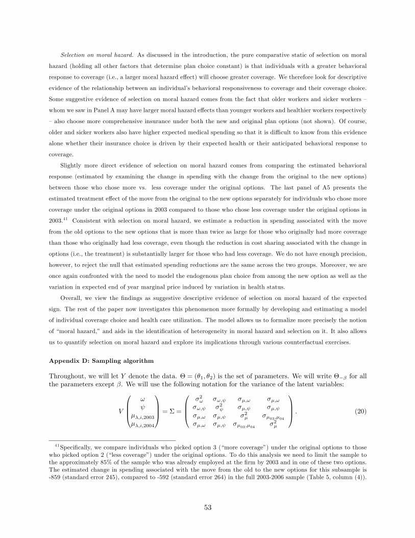
Selection on moral hazard. As discussed in the introduction, the pure comparative static of selection on moral

hazard (holding all other factors that determine plan choice constant) is that individuals with a greater behavioral

response to coverage (i.e., a larger moral hazard e¤ect) will choose greater coverage. We therefore look for descriptive

evidence of the relationship between an individual�s behavioral responsiveness to coverage and their coverage choice.

Some suggestive evidence of selection on moral hazard comes from the fact that older workers and sicker workers �

whom we saw in Panel A may have larger moral hazard e¤ects than younger workers and healthier workers respectively

�also choose more comprehensive insurance under both the new and original plan options (not shown). Of course,

older and sicker workers also have higher expected medical spending so that it is di¢ cult to know from this evidence

alone whether their insurance choice is driven by their expected health or their anticipated behavioral response to

coverage.

Slightly more direct evidence of selection on moral hazard comes from comparing the estimated behavioral

response (estimated by examining the change in spending with the change from the original to the new options)

between those who chose more vs. less coverage under the original options. The last panel of A5 presents the

estimated treatment e¤ect of the move from the original to the new options separately for individuals who chose more

coverage under the original options in 2003 compared to those who chose less coverage under the original options in

2003.41 Consistent with selection on moral hazard, we estimate a reduction in spending associated with the move

from the old options to the new options that is more than twice as large for those who originally had more coverage

than those who originally had less coverage, even though the reduction in cost sharing associated with the change in

options (i.e., the treatment) is substantially larger for those who had less coverage. We do not have enough precision,

however, to reject the null that estimated spending reductions are the same across the two groups. Moreover, we are

once again confronted with the need to model the endogenous plan choice from among the new option as well as the

variation in expected end of year marginal price induced by variation in health status.

Overall, we view the �ndings as suggestive descriptive evidence of selection on moral hazard of the expected

sign. The rest of the paper now investigates this phenomenon more formally by developing and estimating a model

of individual coverage choice and health care utilization. The model allows us to formalize more precisely the notion

of �moral hazard,�and aids in the identi�cation of heterogeneity in moral hazard and selection on it. It also allows

us to quantify selection on moral hazard and explore its implications through various counterfactual exercises.

Appendix D: Sampling algorithm

Throughout, we will let Y denote the data. � = (�1; �2) is the set of parameters. We will write ��� for allthe parameters except �. We will use the following notation for the variance of the latent variables:

V

0BB@!

��;i;2003��;i;2004

1CCA = � =

0BB@�2! �!; ��;! ��;!�!; �2 ��; ��; ��;! ��; �2� ��03;�04��;! ��; ��03;�04 �2�

1CCA : (20)

41Speci�cally, we compare individuals who picked option 3 (�more coverage�) under the original options to thosewho picked option 2 (�less coverage�) under the original options. To do this analysis we need to limit the sample tothe approximately 85% of the sample who was already employed at the �rm by 2003 and in one of these two options.The estimated change in spending associated with the move from the old to the new options for this subsample is-859 (standard error 245), compared to -592 (standard error 264) in the full 2003-2006 sample (Table 5, column (4)).

53

Suppose now that we have some initial draws of the parameters. We sample each parameter conditional

on the others and the data as follows.

� Draw � = (�!; � ; ��; ��)j��� ; !i; i; �it; �it; �i; Y . Given !i; i; �it; �it; �i; �i, the vector � does notenter the density of the data. Spending depends only on (�it; !i) and plan choices depend only on(��;it; �i; �i; !i; i). Therefore, the distribution of �j��� ; !i; i; �it; ��;it; ; �i; �i; Y does not dependon Y . Leaving out the prior for now, the posterior of � is:

f(�j��� ; !i; i; �it; ��;it; �i; �i) /NYi=1

f(�itj��;it; �i; !i; i; ��� ; �)f(��;it; �i; !i; ij��� ; �) (21)

/NYi=1

e� 12

�log(�it��i)��i

�i

�2exp

��12(ui � xi�)0�1(ui � xi�)

�f(�ijk; �)

/ exp��12(� � �̂)0

�X 0�1 IN )X

�(� � �̂)

�where

ui =(log!i; log i; �i;2003; �i;2004; �i) U|{z}5N�1

=

0@log!log �

1A (22)

�|{z}k!+k +k�+k��1

=[�!; � ; ��; ��] X|{z}5N�k!+k +k�+k�

=diag�x!; x ;

�x�2003x�2004

�; x��

and�̂ =

�X 0�1 IN )X

��1 �X 0�1 IN )U

�(23)

Hence, with a di¤use prior, the posterior of � is simply

N(�̂;�X 0�1 IN )X

��1) (24)

With a N(�0; V0) prior, the posterior of � would be

N(��;�X 0�1 IN )X + V �10

��1) (25)

with�� =

�X 0�1 IN )X + V �10

��1 �X 0�1 IN )U�̂ + V �10 �0

�(26)

� Draw �j���; Y . In order to impose the restrictions on � above (for example, that cov(��;2003; !) =cov(��;2004; !) and cov(��;2003; ) = cov(��;2004; )), we sample � in various pieces. To do this, it isuseful to de�ne � as the coe¢ cient from regressing ��;it � x�it�� on log! � x!�! and log � x � .That is,

� =

��!�

�=

��2! �!; �!; �2

��1��!;�� ;�

�(27)

Using this notation, we can write

��;it � x�it�� = �!(log!i � x!i �!) + � (log i � x i � ) + �it (28)

Where �it is normally distributed and independent of log!�x!�! and log �x � . We parameterizethe variance of (�i;2003; �i;2004) as

V

��i;2003�i;2004

�=

�2�1� �2

�1 �� 1

�(29)

54

That is, we think of � as coming from an AR(1) process. Note that for T = 2, as in our baseline model,

specifying that � follows an AR(1) process carries no restriction �we could just as well simply say that

� has some variance matrix. However, our sampling algorithm and code are written for generic T , and

for T � 3, the AR(1) assumption is a meaningful restriction.

�Draw �!; =��2! �!; �!; �2

�j���; Y . As above, the posterior of �!; given the latent variables

and the data does not depend on the data. Standard calculations show that if the prior for �!; is IW (A;m) then its posterior is IW

�n�̂!; +A;n+m

�where

�̂!; =1

n

X�log!i � x!i �!log i � x

i �

��log!i � x!i �!log i � x

i �

�0(30)

�Draw �j���; !i; i; �it; �i; �i; Y . As above, the posterior of � given the latent variables and thedata does not depend on the data. Ignoring any prior for now, the posterior is

f(�)j���; !i; i; �it; �i; �i) /NYi=1

TYt=1

f(�itj�i; �i; !i; i;���; �!; )� (31)

� f(�ij!i; i;���!; ; �)f(�ijk; �)f(!i; ij�)

/NYi=1

TYt=1

exp

0@�12

~yit � ~xi�

��=p1� �2

!21Awhere ~yit = (�it � x�it��) and ~xi =

�log!i � x!i �!log i � x

i �

�. The usual calculations would show that if

the prior for � is N(b0; V0), then the posterior is:

N��(1� �2)��2� X 0X + V0

��1 �(1� �2)��2� X 0Y + V0b0

�;�(1� �2)��2� X 0X + V0

��1�(32)

where X is (~x1; :::; ~xN )0 repeated twice, and Y is (~y1;2003; ::; ~yN;2003; ~y1;2004; :::; ~yN;2004)0.

�Draw �2� j���2� ; !i; i; �it; �i; �i; Y . The same reasoning as for � shows that with a �(a1; a2)prior, the posterior of ��2� is �

�N + a1; 1=

�1��22

Pit(~yit � ~xi�!; )2 + 1=a2

��.

�Draw �j���; �it!i; i; �it; �i; Y . As above, the posterior of � given the latent variables and thedata does not depend on the data. The distribution of � given the latent variables is proportionalto

f(�j�it!i; i; �it; �i;���) /Yi;t

f(�itj�; !i; i;���) (33)

/NYi=1

p1� �2 exp(�1

2(1� �2)�2i1)

TYt=2

exp

��12(�it � ��i;t�1)2

�

/(1� �2)N=2 exp"�12(�� �̂)0

NXi=1

TXt=2

�2i;t�1

!(�� �̂)

#

where �̂ =PNi=1 �i1

2+2PTt=2 �it�it�1

2PNi=1

PTt=2 �

2it�1

, so � has the density of a normal truncated to [�1; 1] andscaled by (1� �2)N=2. 42 We sample from it using a metropolis sampler with candidate density,

N��current ; N

�1=2�

(34)

42We tried to sample from this density using rejection sampling. We drew �� � TN(�̂; v�;�1; 1) and accepted withprobability (1� �2)N=2, unfortunately this leads to unacceptably low acceptance rates.

55

This leads to an acceptance rate between 0.3 and 0.5 for a wide range of sample sizes.

� Draw �it; !ij���;�!; Y . This means drawing �; ! from the region that rationalizes the observed choicesand spending. The likelihood of the latent variables given spending m and choice j is:

f(�i; !ij���;�!) /TYt=1

e�12 (

log �it��it�i

)2e�

�12 (

log!i�moi

so )21(j�(!; ; �; �; �) = j)1(m�(�; !) = m) (35)

where moi = x!i �! + (�i � x�i ��)�� + (log � x i � )� and s

o =q�2! � S!;(�; )��1�; S(�; );! with

� = ��1�; S(�; );! and S(�; );! the vector of covariances between ! and (�; ) and ��; the varianceof (�; ). We can do accept-reject sampling to sample from the region where j�(!; ; �; �; �) = J .However, the area where m�(�; !) = m has measure zero, so accept-reject sampling will not work.Instead, we have to more carefully characterize spending(�; !) to sample from the appropriate area.Let d be the chosen plan�s deductible, x the maximum out of pocket sending, and c the copaymentrate. A person chooses m to maximize utility:

maxm(m� �)� 1

2!(m� �)2

8><>:m m < d

d+ c(m� d) m � d& d+ c(m� d) < x

x d+ c(m� d) � x

(36)

There are four possible solutions for m: 0, �, �+(1� c)!, and �+!. We check whether each of thesesatisfy the constraints in (36) and compare the utilities of the ones that do.

We sample from the distribution of the latent variables subject to m�(�; !) = m using a Metropolis-Hastings sampler. The density of !i given mit is

f(!ijfmitg;moi ; s

o)proptoe��12 (

log!i�moi

so )2TYt=1

0BBBB@1fm = 0gP (m = 0j!)

+1f0 < m < dgP (m = mitj!)

+1fd < m < xg 1mit�(1�c)! e

�12

�log(mit�(1�c)!i)���;it

�i

�2+1fm > xg+ 1fx < mg 1

mit�! e�12

�log(mit�!i)���;it

�i

�2

1CCCCA(37)

We sample from this density by:

1. Sample

! � ~f(!j:::) / e��12 (

log!i�moi

so )2TYt=1

2641fd < m < xg 1mit�(1�c)! e

�12

�log(mit�(1�c)!i)���;it

��;i

�2

+1fx < mg 1mit�! e

�12

�log(mit�!i)���;it

��;i

�2375 (38)

We sample from this density using the Metropolis-Hastings algorithm with a normal candidate

density for log!. For each draw of !i, we run �ve metropolis iterations.

2. If mit = 0 for any t, draw log �it � N(��;it; ��;i).

3. If 0 < mit < d, set �it = mit

4. Accept !i if the observed mit is the solution to (36) and jit = j�(!i; i; ��;it; ��;i; �i) for all t,

else repeat.

� For t = 2003; 2004, draw �itj���; Y . The posterior is a normal distribution truncated to the regionwhere the choices implied by the model match the choices in the data. We repeatedly draw from this

56

normal distribution until the choices match. The joint distribution of log i; log!i; f�isg; log(�it��i)is normal with mean (x i � ; x

i!�!; fx�is��g; x�it��) and variance

Vi =

0BBBB@ �

0BB@�!;�� ;��2��2�

1CCA��!;� � ;� �2� �2�

��2i + �

2�

1CCCCA (39)

Note that we do not need to condition on log �is for s 6= t, because conditional on �is, �it and log �isare independent. Let C�t;(!; ;�s;�t) be the vector of covariances between �it and the other latentvariables, V��t;i be Vi with the row and column for �it deleted, and

ei =

0BB@log!ilog i�is�it

1CCA�0BB@xi!�!x i � xis� ��xit���

1CCA (40)

The posterior mean of �it is then ei�i with �i = C�t;(!; ;�s;�)V�1��t;i, and the variance is �

2� �

C�t;(!; ;�s;�)V�1��t;iC

0�t;(!; ;�s;�)

.

� Draw ij�� ; Y . As with �it, the posterior will be a normal distribution truncated to the regionwhere the choices implied by the model match the choices in the data. We repeatedly draw from thisnormal distribution until the choices match. De�ne ei as when sampling �it, but leave out �it. Also,let C ;(!;�) be the vector of covariances of and (!; �) and �� be � with the row and column for removed. Then, the posterior distribution of is

N�ei�

�1� C ;(!;�)0 ; �

2 � C ;(!;�)��1� C

0 ;(!;�)

�(41)

� Draw �ij���i ; Y .

f(�ij log �it; �i; �; k) /1f�2 < ��2g 1

�2(k�1)e��

�2=�Yt

1

�e� 12

�log �it��

�i

�2(42)

/1f�2 < ��2g 1

�2(k�1+T=2)e��

�2(1=�+ 12

Pt(log �it��i)

2)

So the posterior of ��2i is �(k+T=2; 2�2+�

Pt(log �it��i)2

)1f�2i < ��2, a truncated Gamma distribution.

� Draw 1j�� 1 ; Y; :::.

f( 1j�i; k; Y; :::) /Y

f(�ij 1; k)p( 1) (43)

/Y

��2(k�1)i

e���2i = 1

k1�(k)

1

1� F�(���2; k; 1)p( 1)

/(1� F�(���2; k; 1))�N (1= 1)Nke�(1= 1)P��2i p( 1)

/(1= 1)Nk+k0�1e�(1= 1)

1;0P��2i

+1

1;0 � (1� F�(���2; k; 1))�N

where the prior for 1= 1 is �(k0; 1;0). This is a gamma distribution times some weighting function.

Therefore, we use a metropolis sampler with candidate density for 1= 1 a �(Nk + k0; 1;0

1;0P��2i +1

).

Given the current estimates, 1�F�(���2; k; 1) is very close to one, so this metropolis sampler acceptsnearly all draws.

57

� Draw 2j�� 2 ; Y .

f(kj�i; �; :::) /Y

��2(k�1)i

e���2i =�

�k�(k)p(k)(1� F�(���2; k; �))�N (44)

/ekPlog ��2i +log ��N

�(k)Np(k)(1� F�(���2; k; �))�N

which is a nonstandard distribution. We use the adaptive rejection metropolis sampling (ARMS)

method of Gilks, Best, and Tan (1995) to sample from it. This is a hybrid accept-reject and metropolis

sampling scheme. It is designed to sample from log-concave and nearly log-concave densities e¢ ciently.

Without the (1 � F�(���2; k; �))�N term, this density would be log-concave (it may be log-concave

anyway), and ARMS can sample from it very e¢ ciently.

Appendix E: Heterogeneity in moral hazard in a �multiplicative model�

To explore whether our �ndings of substantial heterogeneity in moral hazard are simply an artifact of the additive

way that moral hazard a¤ect utilization in the model of Section I, we estimated a slightly modi�ed model, in which

moral hazard enters multiplicatively. Speci�cally, we use the same model and econometric speci�cation, except that

we replace equation (1) with the following expression:

u(m;�; !; j) =

�(m� �)� 1

2!�(m� �)2

�+hy � cj(m)� pj

i: (45)

That is, we keep the utility function speci�cation the same, except that we add � to the denominator of the second

component. One can check that this small modi�cation implies, in the context of a linear contract, that optimal

utilization is given by

m�(�; !; c) =max [0; �(1 + !(1� c))] : (46)

That is, ! now a¤ects the optimal spending multiplicatively, rather than additively as in equation (3). Note that

in this alternative model, �moral hazard�� i.e. the di¤erence in spending between no insurance (c = 1) and full

insurance (c = 0) �is now �! rather than ! as in the original model; as a result, when choosing insurance one�s

moral hazard type is uncertain. The rest of the model speci�cation remains the same.

Appendix Tables A6 and A7 report the results from the estimation of this multiplicative model. The tables

correspond to Table 7(a) and Table 9 in the main text. As one can observe, the qualitative features of the results

remain similar. For example, the heterogeneity in ! is still substantial, with a coe¢ cient of variation of about 2.5

(bottom of Appendix Table A6), and the qualitative pattern reported in Appendix Table A7 is quite similar, although

slightly smaller, to the pattern shown in Table 9 of the main text.

Appendix F: Robustness checks of the main, model-based �ndings.

Appendix Table A8 brie�y explores the robustness of some of our main �ndings to alternative econometric speci�ca-

tions of the baseline model. Overall, we �nd that the main results are quite stable across alternative speci�cations.

All the alternative speci�cations we explore give rise to quantitatively similar estimates of average moral hazard

(column (1)), heterogeneity in moral hazard (column (2)), selection on moral hazard (column (4)), the implications of

accounting for selection on moral hazard for the spending reduction that can be achieved by o¤ering a high deductible

58

plan (column (5) vs. column (1)), and the contribution of selection on moral hazard to the overall welfare cost of

adverse selection (columns (7) relative to column (6)).

The �rst row replicates our baseline �ndings reported earlier. The next two rows explore the sensitivity of our

�ndings to trying to account for various institutional features that our baseline speci�cation abstracted from. Row

2 explores the sensitivity of our �ndings to trying to account for the fact that the lowest coverage option under the

new options (option 1) has a health reimbursement account (HRA) component (see Section II for details) which we

abstracted from in our econometric speci�cation. To do so, we simply drop from the sample the 2004 observations

associated with employees who chose option 1 when o¤ered the new choice set (roughly 6% of those o¤ered the new

choice set).

Row 3 provides one way of gauging the potential importance of �passive choices�for our results. As noted earlier,

an attraction of our setting is that for employees who are o¤ered the new choice set in 2004, there is no option of

staying with their existing plan. However, there were defaults for those who did not make an �active�choice under

the new options. To account for �and exclude �a set of potentially passive choosers, we identi�ed all individuals

whose coverage choices under the new bene�t options for each of �ve di¤erent insurance options (health, drug, dental,

short-term disability, and long-term disability) are consistent with the defaults for those �ve options.43 Row 3 shows

the results of excluding the 2004 observations for the approximately 12% of individuals o¤ered the new options for

whom all of their coverage decisions are consistent with the default options.

The remaining rows of the table investigate the sensitivity of our �ndings to some alternative natural parame-

terizations of the model. In row 4 we remove all of the demographic covariates from the model (i.e., age, gender, job

tenure, income, and health risk score) leaving only indicator variables for year and treatment group (to capture the

quasi-experimental variation in the option set) and coverage tier dummies (because the prices of the options depend

on coverage tier). In row 5 we allow for heteroskedastic errors, by letting all the parameters in the variance-covariance

matrix (see equation (8)) depend on all the covariates. In row 6, instead of assuming that log!i, log i, and ��;i

are drawn from a joint normal distribution, we assume that they are drawn from a mixture of two normals.

While there is, of course, a potentially limitless set of alternative speci�cations one could investigate, we found the

stability of the core results to the natural ones we tried reassuring about the stability of our model estimates within

our context. As noted previously, whether or not the results would generalize �quantitatively or even qualitatively �

to other option sets, populations, or di¤erent models of coverage choice and utilization �is of course an open question.

43Employees make their choices for each insurance domain all at the same time, on the same bene�t worksheet duringopen enrollment period. Einav, Finkelstein, Pascu, and Cullen (forthcoming) provide more detail and discussion ofthese other bene�ts options and choices.

59

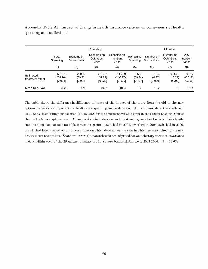
Appendix Table A1: Impact of change in health insurance options on components of healthspending and utilization

TotalSpending

Spending onDoctor Visits

Spending onOutpatient

Visits

Spending onInpatient

Visits

RemainingSpending

Number ofDoctor Visits

Number ofOutpatient

Visits

AnyInpatient

Visits

(1) (2) (3) (4) (5) (6) (7) (8)

­591.81 ­220.37 ­310.32 ­116.69 55.91 ­1.94 ­0.0005 ­0.017(264.26) (69.32) (137.89) (246.17) (69.34) (0.37) (0.27) (0.011)

[0.034] [0.004] [0.033] [0.639] [0.427] [0.000] [0.999] [0.155]

Mean Dep.  Var. 5392 1475 1922 1804 191 12.2 3 0.14

UtilizationSpending

Estimatedtreatment effect

The table shows the di¤erence-in-di¤erence estimate of the impact of the move from the old to the new

options on various components of health care spending and utilization. All columns show the coe¢ cient

on TREAT from estimating equation (17) by OLS for the dependent variable given in the column heading. Unit of

observation is an employee-year. All regressions include year and treatment group �xed e¤ects. We classify

employees into one of four possible treatment groups - switched in 2004, switched in 2005, switched in 2006,

or switched later - based on his union a¢ liation which determines the year in which he is switched to the new

health insurance options. Standard errors (in parentheses) are adjusted for an arbitrary variance-covariance

matrix within each of the 28 unions; p-values are in [square brackets].Sample is 2003-2006. N = 14,638.

60

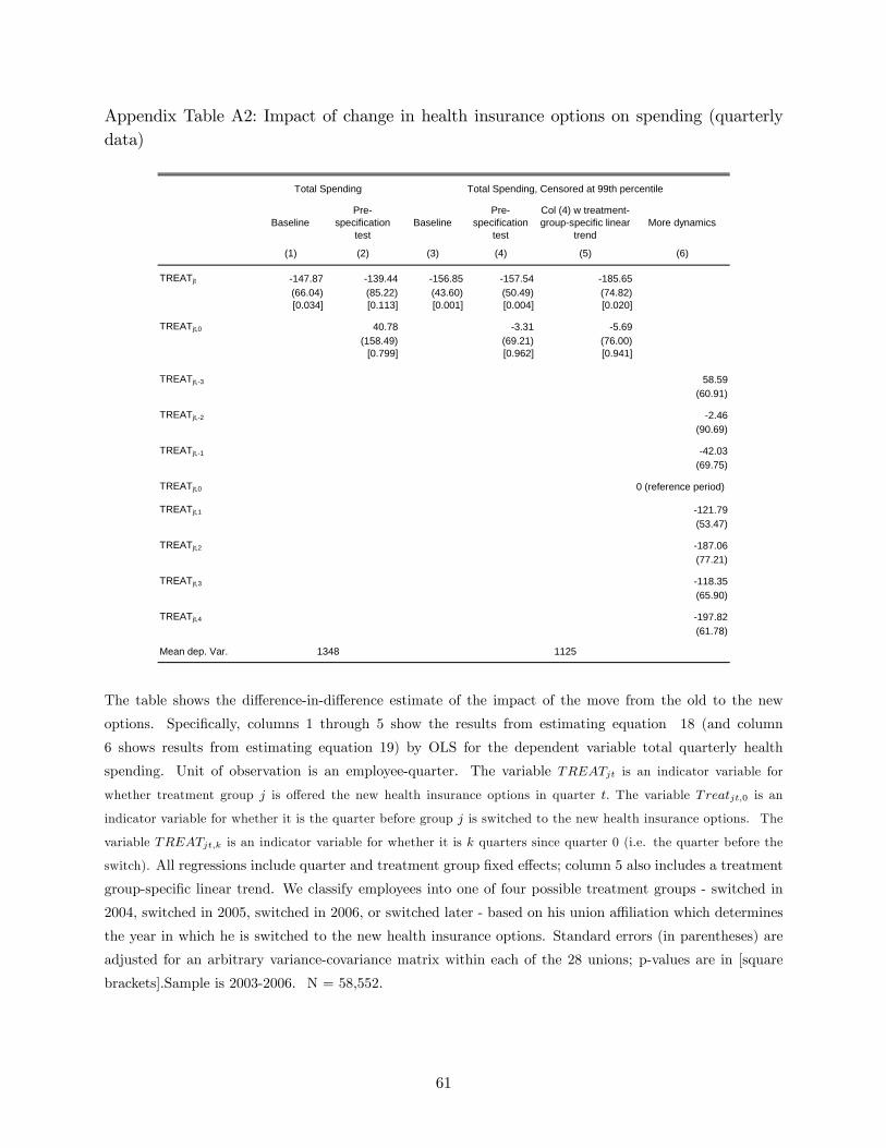
Appendix Table A2: Impact of change in health insurance options on spending (quarterlydata)

BaselinePre­

specificationtest

BaselinePre­

specificationtest

Col (4) w treatment­group­specific linear

trendMore dynamics

(1) (2) (3) (4) (5) (6)

TREATjt ­147.87 ­139.44 ­156.85 ­157.54 ­185.65(66.04) (85.22) (43.60) (50.49) (74.82)[0.034] [0.113] [0.001] [0.004] [0.020]

TREATjt,0 40.78 ­3.31 ­5.69(158.49) (69.21) (76.00)

[0.799] [0.962] [0.941]

TREATjt,­3 58.59(60.91)

TREATjt,­2 ­2.46(90.69)

TREATjt,­1 ­42.03(69.75)

TREATjt,0 0 (reference period)

TREATjt,1 ­121.79(53.47)

TREATjt,2 ­187.06(77.21)

TREATjt,3 ­118.35(65.90)

TREATjt,4 ­197.82(61.78)

Mean dep. Var.

Total Spending

1348

Total Spending, Censored at 99th percentile

1125

The table shows the di¤erence-in-di¤erence estimate of the impact of the move from the old to the new

options. Speci�cally, columns 1 through 5 show the results from estimating equation 18 (and column

6 shows results from estimating equation 19) by OLS for the dependent variable total quarterly health

spending. Unit of observation is an employee-quarter. The variable TREATjt is an indicator variable for

whether treatment group j is o¤ered the new health insurance options in quarter t: The variable Treatjt;0 is an

indicator variable for whether it is the quarter before group j is switched to the new health insurance options. The

variable TREATjt;k is an indicator variable for whether it is k quarters since quarter 0 (i.e. the quarter before the

switch). All regressions include quarter and treatment group �xed e¤ects; column 5 also includes a treatment

group-speci�c linear trend. We classify employees into one of four possible treatment groups - switched in

2004, switched in 2005, switched in 2006, or switched later - based on his union a¢ liation which determines

the year in which he is switched to the new health insurance options. Standard errors (in parentheses) are

adjusted for an arbitrary variance-covariance matrix within each of the 28 unions; p-values are in [square

brackets].Sample is 2003-2006. N = 58,552.

61

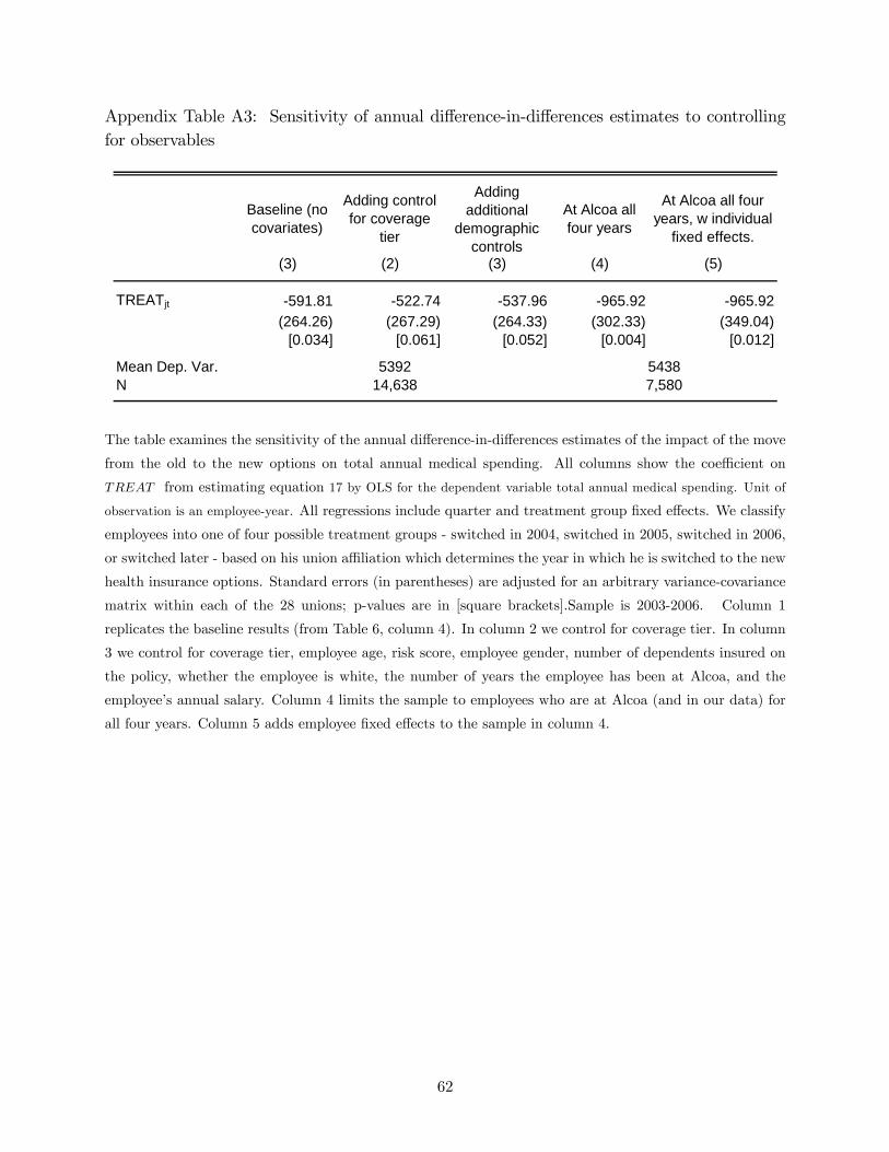
Appendix Table A3: Sensitivity of annual di¤erence-in-di¤erences estimates to controllingfor observables

Baseline (nocovariates)

Adding controlfor coverage

tier

Addingadditional

demographiccontrols

At Alcoa allfour years

At Alcoa all fouryears, w individual

fixed effects.

(3) (2) (3) (4) (5)

TREATjt ­591.81 ­522.74 ­537.96 ­965.92 ­965.92(264.26) (267.29) (264.33) (302.33) (349.04)

[0.034] [0.061] [0.052] [0.004] [0.012]

Mean Dep. Var.N

539214,638 7,580

5438

The table examines the sensitivity of the annual di¤erence-in-di¤erences estimates of the impact of the move

from the old to the new options on total annual medical spending. All columns show the coe¢ cient on

TREAT from estimating equation 17 by OLS for the dependent variable total annual medical spending. Unit of

observation is an employee-year. All regressions include quarter and treatment group �xed e¤ects. We classify

employees into one of four possible treatment groups - switched in 2004, switched in 2005, switched in 2006,

or switched later - based on his union a¢ liation which determines the year in which he is switched to the new

health insurance options. Standard errors (in parentheses) are adjusted for an arbitrary variance-covariance

matrix within each of the 28 unions; p-values are in [square brackets].Sample is 2003-2006. Column 1

replicates the baseline results (from Table 6, column 4). In column 2 we control for coverage tier. In column

3 we control for coverage tier, employee age, risk score, employee gender, number of dependents insured on

the policy, whether the employee is white, the number of years the employee has been at Alcoa, and the

employee�s annual salary. Column 4 limits the sample to employees who are at Alcoa (and in our data) for

all four years. Column 5 adds employee �xed e¤ects to the sample in column 4.

62

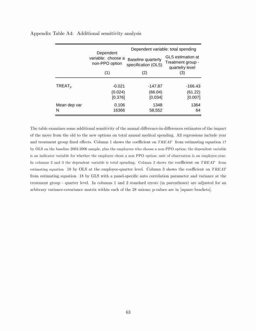
Appendix Table A4: Additional sensitivity analysis

Baseline quarterlyspecification (OLS)

GLS estimation atTreatment group ­

quartelry level(1) (2) (3)

TREATjt ­0.021 ­147.87 ­166.43(0.024) (66.04) (61.22)[0.376] [0.034] [0.007]

Mean dep var 0.106 1348 1364N 16366 58,552 64

Dependentvariable:  choose a

non­PPO option

Dependent variable: total spending

The table examines some additional sensitivity of the annual di¤erence-in-di¤erences estimates of the impact

of the move from the old to the new options on total annual medical spending. All regressions include year

and treatment group �xed e¤ects. Column 1 shows the coe¢ cient on TREAT from estimating equation 17

by OLS on the baseline 2003-2006 sample, plus the employees who choose a non-PPO option; the dependent variable

is an indicator variable for whether the employee chose a non PPO option; unit of observation is an employee-year.

In columns 2 and 3 the dependent variable is total spending. Column 2 shows the coe¢ cient on TREAT from

estimating equation 18 by OLS at the employee-quarter level. Column 3 shows the coe¢ cient on TREAT

from estimating equation 18 by GLS with a panel-speci�c auto correlation parameter and variance at the

treatment group - quarter level. In columns 1 and 2 standard errors (in parentheses) are adjusted for an

arbitrary variance-covariance matrix within each of the 28 unions; p-values are in [square brackets].

63

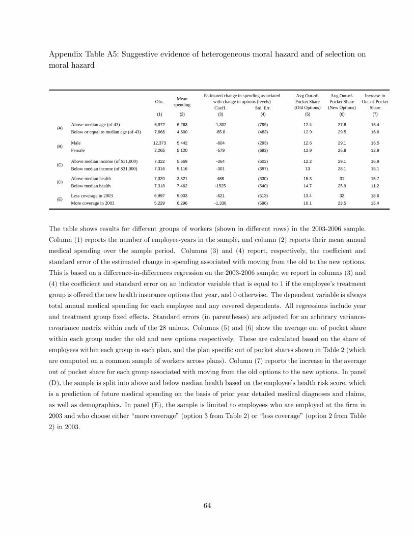
Appendix Table A5: Suggestive evidence of heterogeneous moral hazard and of selection onmoral hazard

Coeff. Std. Err.(1) (2) (3) (4) (5) (6) (7)

Above median age (of 43) 6,972 6,263 ­1,302 (799) 12.4 27.8 15.4

Below or equal to median age (of 43) 7,666 4,600 ­85.8 (483) 12.9 29.5 16.6

Male 12,373 5,442 ­604 (293) 12.6 29.1 16.5

Female 2,265 5,120 ­579 (693) 12.9 25.8 12.9

Above median income (of $31,000) 7,322 5,669 ­364 (602) 12.2 29.1 16.9

Below median income (of $31,000) 7,316 5,116 ­301 (397) 13 28.1 15.1

Above median health 7,320 3,321 488 (330) 15.3 31 15.7

Below median health 7,318 7,462 ­1525 (540) 14.7 25.9 11.2

Less coverage in 2003 6,997 5,003 ­621 (513) 13.4 32 18.6

More coverage in 2003 5,229 6,296 ­1,336 (596) 10.1 23.5 13.4

Obs. Meanspending

Avg Out­of­Pocket Share(Old Options)

Increase inOut­of­Pocket

Share

Avg Out­of­Pocket Share

(New Options)

Estimated change in spending associatedwith change in options (levels)

(A)

(B)

(D)

(C)

(E)

The table shows results for di¤erent groups of workers (shown in di¤erent rows) in the 2003-2006 sample.

Column (1) reports the number of employee-years in the sample, and column (2) reports their mean annual

medical spending over the sample period. Columns (3) and (4) report, respectively, the coe¢ cient and

standard error of the estimated change in spending associated with moving from the old to the new options.

This is based on a di¤erence-in-di¤erences regression on the 2003-2006 sample; we report in columns (3) and

(4) the coe¢ cient and standard error on an indicator variable that is equal to 1 if the employee�s treatment

group is o¤ered the new health insurance options that year, and 0 otherwise. The dependent variable is always

total annual medical spending for each employee and any covered dependents. All regressions include year

and treatment group �xed e¤ects. Standard errors (in parentheses) are adjusted for an arbitrary variance-

covariance matrix within each of the 28 unions. Columns (5) and (6) show the average out of pocket share

within each group under the old and new options respectively. These are calculated based on the share of

employees within each group in each plan, and the plan speci�c out of pocket shares shown in Table 2 (which

are computed on a common sample of workers across plans). Column (7) reports the increase in the average

out of pocket share for each group associated with moving from the old options to the new options. In panel

(D), the sample is split into above and below median health based on the employee�s health risk score, which

is a prediction of future medical spending on the basis of prior year detailed medical diagnoses and claims,

as well as demographics. In panel (E), the sample is limited to employees who are employed at the �rm in

2003 and who choose either �more coverage�(option 3 from Table 2) or �less coverage�(option 2 from Table

2) in 2003.

64

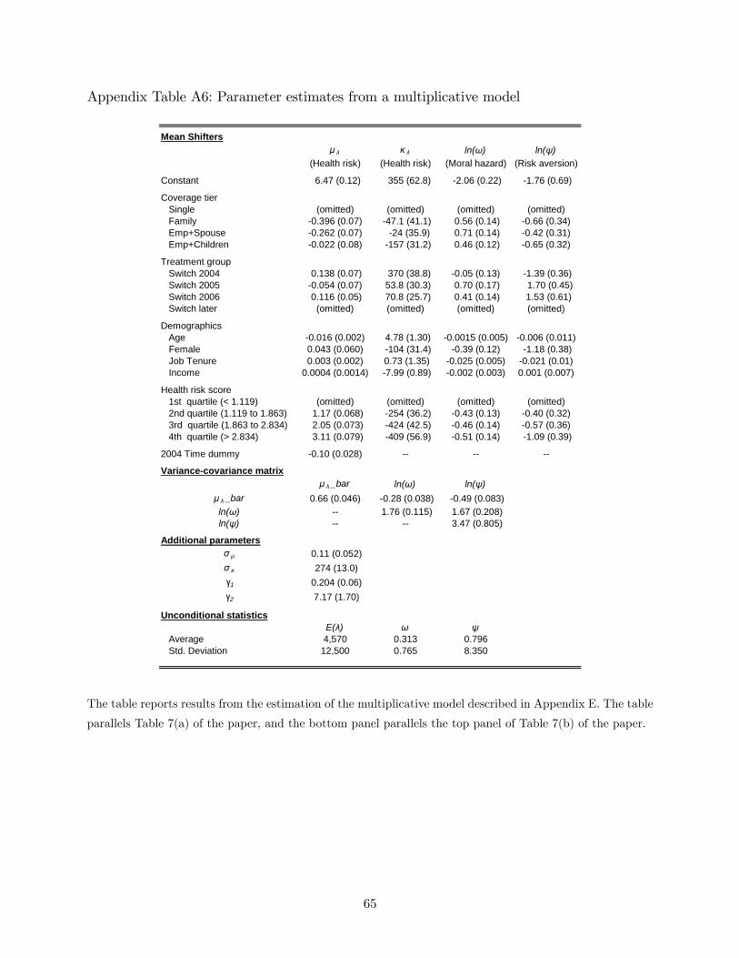
Appendix Table A6: Parameter estimates from a multiplicative model

Mean Shiftersμ λ κ λ ln(ω) ln(ψ)

(Health risk) (Health risk) (Moral hazard) (Risk aversion)

Constant    6.47 (0.12)     355 (62.8)   ­2.06 (0.22)   ­1.76 (0.69)

Coverage tier   Single (omitted) (omitted) (omitted) (omitted)   Family  ­0.396 (0.07)   ­47.1 (41.1)   0.56 (0.14)  ­0.66 (0.34)   Emp+Spouse  ­0.262 (0.07)     ­24 (35.9)   0.71 (0.14)  ­0.42 (0.31)   Emp+Children  ­0.022 (0.08)    ­157 (31.2)   0.46 (0.12)  ­0.65 (0.32)

Treatment group   Switch 2004   0.138 (0.07)     370 (38.8)  ­0.05 (0.13)   ­1.39 (0.36)   Switch 2005  ­0.054 (0.07)    53.8 (30.3)   0.70 (0.17)     1.70 (0.45)   Switch 2006   0.116 (0.05)    70.8 (25.7)   0.41 (0.14)    1.53 (0.61)   Switch later (omitted) (omitted) (omitted) (omitted)

DemographicsAge  ­0.016 (0.002)     4.78 (1.30)  ­0.0015 (0.005)  ­0.006 (0.011)Female  0.043 (0.060)     ­104 (31.4)  ­0.39 (0.12)   ­1.18 (0.38)Job Tenure  0.003 (0.002)   0.73 (1.35)   ­0.025 (0.005)   ­0.021 (0.01)Income  0.0004 (0.0014)   ­7.99 (0.89)   ­0.002 (0.003)   0.001 (0.007)

Health risk score   1st  quartile (< 1.119) (omitted) (omitted) (omitted) (omitted)   2nd quartile (1.119 to 1.863)    1.17 (0.068)    ­254 (36.2)  ­0.43 (0.13)  ­0.40 (0.32)   3rd  quartile (1.863 to 2.834)    2.05 (0.073)    ­424 (42.5)  ­0.46 (0.14)  ­0.57 (0.36)   4th  quartile (> 2.834)    3.11 (0.079)    ­409 (56.9)  ­0.51 (0.14)   ­1.09 (0.39)

2004 Time dummy  ­0.10 (0.028) ­­ ­­ ­­

Variance­covariance matrixμ λ _bar ln(ω) ln(ψ)

μ λ _bar  0.66 (0.046)  ­0.28 (0.038)  ­0.49 (0.083)ln(ω)  ­­  1.76 (0.115)  1.67 (0.208)ln(ψ)  ­­  ­­  3.47 (0.805)

Additional parametersσ μ  0.11 (0.052)σ κ  274 (13.0) γ1  0.204 (0.06)γ2  7.17 (1.70)

Unconditional statisticsE(λ) ω ψ

   Average 4,570 0.313 0.796   Std. Deviation 12,500 0.765 8.350

The table reports results from the estimation of the multiplicative model described in Appendix E. The table

parallels Table 7(a) of the paper, and the bottom panel parallels the top panel of Table 7(b) of the paper.

65

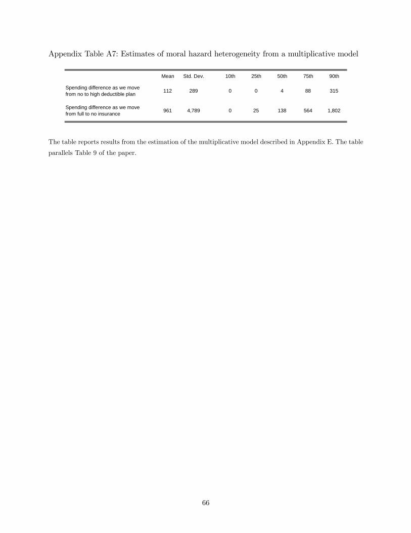
Appendix Table A7: Estimates of moral hazard heterogeneity from a multiplicative model

Mean Std. Dev. 10th 25th 50th 75th 90th

Spending difference as we movefrom no to high deductible plan 112 289 0 0 4 88 315

Spending difference as we movefrom full to no insurance 961 4,789 0 25 138 564 1,802

The table reports results from the estimation of the multiplicative model described in Appendix E. The table

parallels Table 9 of the paper.

66

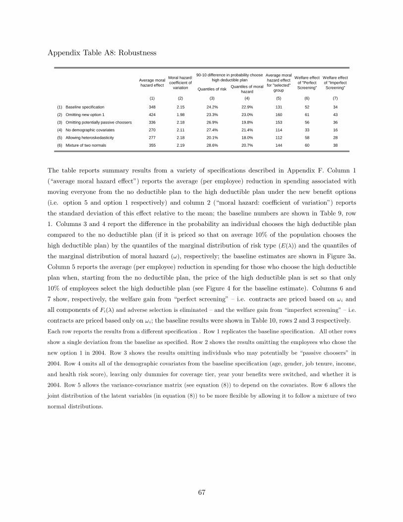
Appendix Table A8: Robustness

Quantiles of risk Quantiles of moralhazard

(1) (2) (3) (4) (5) (6) (7)

(1) Baseline specification 348 2.15 24.2% 22.9% 131 52 34

(2) Omitting new option 1 424 1.98 23.3% 23.0% 160 61 43

(3) Omitting potentially passive choosers 336 2.18 26.9% 19.8% 153 56 36

(4) No demographic covariates 270 2.11 27.4% 21.4% 114 33 16

(5) Allowing heteroskedasticity 277 2.18 20.1% 18.0% 112 58 28

(6) Mixture of two normals 355 2.19 28.6% 20.7% 144 60 38

Average moralhazard effect

Moral hazard:coefficient of

variation

90­10 difference in probability choosehigh deductible plan

Average moralhazard effectfor "selected"

group

Welfare effectof "PerfectScreening"

Welfare effectof "ImperfectScreening"

The table reports summary results from a variety of speci�cations described in Appendix F. Column 1

(�average moral hazard e¤ect�) reports the average (per employee) reduction in spending associated with

moving everyone from the no deductible plan to the high deductible plan under the new bene�t options

(i.e. option 5 and option 1 respectively) and column 2 (�moral hazard: coe¢ cient of variation�) reports

the standard deviation of this e¤ect relative to the mean; the baseline numbers are shown in Table 9, row

1. Columns 3 and 4 report the di¤erence in the probability an individual chooses the high deductible plan

compared to the no deductible plan (if it is priced so that on average 10% of the population chooses the

high deductible plan) by the quantiles of the marginal distribution of risk type (E(�)) and the quantiles of

the marginal distribution of moral hazard (!), respectively; the baseline estimates are shown in Figure 3a.

Column 5 reports the average (per employee) reduction in spending for those who choose the high deductible

plan when, starting from the no deductible plan, the price of the high deductible plan is set so that only

10% of employees select the high deductible plan (see Figure 4 for the baseline estimate). Columns 6 and

7 show, respectively, the welfare gain from �perfect screening��i.e. contracts are priced based on !i and

all components of Fi(�) and adverse selection is eliminated �and the welfare gain from �imperfect screening��i.e.

contracts are priced based only on !i; the baseline results were shown in Table 10, rows 2 and 3 respectively.

Each row reports the results from a di¤erent speci�cation . Row 1 replicates the baseline speci�cation. All other rows

show a single deviation from the baseline as speci�ed. Row 2 shows the results omitting the employees who chose the

new option 1 in 2004. Row 3 shows the results omitting individuals who may potentially be �passive choosers� in

2004. Row 4 omits all of the demographic covariates from the baseline speci�cation (age, gender, job tenure, income,

and health risk score), leaving only dummies for coverage tier, year your bene�ts were switched, and whether it is

2004. Row 5 allows the variance-covariance matrix (see equation (8)) to depend on the covariates. Row 6 allows the

joint distribution of the latent variables (in equation (8)) to be more �exible by allowing it to follow a mixture of two

normal distributions.

67