Selection bias and auditing policies oninsurance claims

Jean Pinquet

Université de Paris X, U.F.R. de sciences économiques,200 avenue de la République 92001 NANTERRE CEDEXFRANCETél: (33)1 40 97 47 58 Fax: (33)1 40 97 59 73E-Mails: pinquet@u-paris10.fr ; jpinquet@free.fr

with Mercedes Ayuso & Montserrat Guillén

Abstract

Statistical models which lead to optimal auditing policies are subject toselection bias. Indeed, there is a severe discrepancy between the range ofderivation of the risk model (the audited claims) and its range of application(the incoming fraud suspicious claims). This paper applies a classical statisticalmodel (bivariate probit model with censoring) which allows to assess and tocounteract selection bias. The model is applied on a Catalan data base, andconsequences are drawn on the efficiency of audit policies.

Keywords

Bivariate probit model with censoring. Bivariate Gaussian copulas.

1

1 Introduction

Auditing policies derived from statistical analysis and applied to insuranceclaims face a major selection bias problem. A score assessing fraud risk isderived from a regression analysis on audited claims, and is usually applied toall the incoming claims in order to select those which are then recommendedfor audit. This discrepancy between the range of derivation of the risk model(i.e. the audited claims) and its range of application (the incoming claims)creates the selection bias.Random auditing of claims is the basic strategy which makes it possible to

counteract selection bias. A pure random auditing strategy consists in selectingclaims at random, then in auditing these claims. Thanks to this controlledexperiment, all the fraudulent claims in the selected sample will be identifiedas such. The estimation of a single fraud equation in this sample providesan estimated fraud probability for incoming claims which is not subject toselection bias.Random auditing is partly carried out on the data base which we investi-

gated. Twenty percent of the claims are thus selected and recommended foraudit. However, only one claim out of five is eventually audited in this popu-lation (see Section 2 for more details about auditing processes). Selection biasis avoided only if all the non-audited claims can be considered to be definitelynon-fraudulent. Optimal auditing strategies are then designed from the esti-mation of a fraud equation on the audited claims (see Ayuso, Guillén et al.(2004) for derivations with the data base used in this paper).Random auditing is far from being used by all insurance companies. With-

out such a policy, the effect of selection bias on the incoming claims can easilybe anticipated. The experts take an audit decision from claim characteristicsrecorded in the company files, but they are also able to capture idiosyncrasiesin fraud distributions which are not summarized by the observable information.Given observable characteristics, fraud risk is expected to be less important fora claim exempted from audit by the expert than for another one checked forfraud. A fraud risk model derived without taking this selection problem intoaccount would then overestimate fraud probabilities for the incoming claims.Statistical models can offset this bias by using a two equation model. An

audit equation is estimated on all the claims together with another one relatedto fraud, which is estimated only on the audited claims. From a joint distri-bution of the random components in each equation, we can condition fraudrisk not only on claim characteristics but also on whether or not the claim was

2

retained for audit by the claims adjusters. To our knowledge, selection modelshave so far not been applied to claim auditing.Selection models can be designed with or without censoring for the variable

of interest. In our context, data are censored since fraud is checked on theaudited claims only. Selection models with censoring (i.e. those for which thevariable of interest is observed only on the selected individuals) are widelyused in statistical and econometric literature. As regards the pair: selectionvariable and variable of interest, we can cite

• Heckman (1979) for the seminal paper on this topic, and an applicationto the pair: participation in a labor market - hourly wage. The variableof interest is defined from a linear model.

• Hausman, Wise (1979) for a panel data model with endogenous attrition.The selection variable refers to attrition and the variable of interest is awage level.

• Credit scoring models (Hand and Henley (1997)). The problem discussedis very similar to the one addressed in this paper, since the variable ofinterest is binary. The dependent variable refers to credit default, andselection means acceptance of the loan demand. Statistical analysis ofselection bias in this context is often referred to as rejection inference.

Selection does not always imply censoring for the variable of interest. Indealing with public policy evaluation, selection means participation in a pro-gram, an educational program for instance. In this case a variable of interestsuch as the wage level is observed for all the individuals. Statistical analysisleads to a "difference in differences" approach (see Rosenbaum, Rubin (1983),Heckman (2000)).Closer to the subject dealt with in this paper is the two equation model

proposed by Chiappori and Salanié (2000) which tests for asymmetric infor-mation in insurance markets. Two binary variables are explained on insurancecontracts, the coverage level and an accident indicator. Data are analyzedwith a bivariate probit model, and the nullity of the correlation coefficient istested for. This approach is used on our two equation model on audit andfraud. The estimated correlation coefficient is expected to be positive since itreflects the ability of claims adjusters to assess hidden characteristics in frauddistributions.

3

The paper is organized as follows. Section 2 explains how fraud detectionstrategies for automobile insurance claims are implemented in the insurancecompanies. Section 3 describes the data base. Section 4 presents the bivariateprobit model and its application to the correction of selection bias. We considera natural extension of the single equation probit model on the fraud variable(see Belhadji, Dionne, Tarkani (2000) and Artis, Ayuso, Guillén (2003) forthe inclusion of misclassification risk in the fraud equation). Our claims database is split into two populations. Claims selected at random (one out of five)are recommended for audit, whereas there is no specific recommendation forthe other ones. We will use the latter population as the working sample sincethese claims are subject to selection bias. The claims selected at random willbe used as a holdout sample in order to assess the efficiency of the statisticalmodel. The estimated correlation coefficient in the bivariate probit model isfound to be positive on our data. This means that, if we control for observableinformation on claims, fraud risk is lower for claims exempted from audit bythe experts.Optimal auditing policies which take into account selection bias are pre-

sented in Section 5, and concluding remarks appear in Section 6.

2 Fraud detection strategies on automobile in-surance claims and selection bias issues

Applying auditing strategies to fraud detection in the insurance market has notbeen a general practice, but insurers are beginning to realize the advantages ofcontrolling this risk. In most European countries, when an insurer finds a claimwhich shows evidence of fraud, an agreement with the policyholder is usuallyreached. Most settlements end up not renewing the policy and others leadto a reduction of the claim compensation. This situation is in contrast withthe highly litigious US system. However, even if very few fraudulent claimsare discussed in court, many European insurers are beginning to implementstrategies to control fraud.Let us formalize now the selection bias issue. Suppose first that all the

incoming claims can be considered for audit. The selection bias issue can beformalized in the following way: A and F denote the binary variables relatedto audit and fraud, and x is the vector of variables which describe the claim.A statistical model assessing fraud risk is derived on the audited claims and

4

estimates probabilities of the type P (F = 1 |A = 1, x) = E(F |A = 1, x). Nowan audit policy induced by this model is applied on the incoming claims, anduses the probabilities P (F = 1 | x) = E(F | x). Selection bias is a consequenceof the confusion between conditional and unconditional probabilities.In reality all the incoming claims are not likely to be audited. A description

of the audit process will explain why. All the incoming claims are in the firstplace checked by the adjusters. They consider the causes of car damages,circumstances of the accident and policy characteristics. A claim the adjusterdoes not find suspicious will be exempted from audit and settled routinelywhatever the audit strategy. In what follows, audit means that the claim istransferred to a Special Investigation Unit, referred to as an SIU. This unitprovides a further assessment of the claim and decides whether to consider itas fraudulent or not.Hence a variable related to fraud suspicion is created by the adjuster before

the audit decision, and we denote it as S. For this binary variable, we have

S = 0⇒ A = 0. (1)

The condition given in (1) simply means that the audit decision is nested insidethe selection decision induced by S. Since both variables S and A are binary,this condition amounts to A ≤ S. A claim for which S = 1 will be referred tolater as suspicious of fraud. Conversely, S = 0 if the first screening reveals nofraud suspicion. Another reason (although less frequent) which implies S = 0is that no loss is expected, for instance if the insurer of the third party paysfor the car damages or if the deductible exceeds the claim cost.Since only the claims suspected of fraud are likely to be audited, selection

bias now reflects the confusion between P (F = 1 |A = 1, x) and P (F = 1 |S =1, x), under the condition given in (1). This bias increases with the proportionof suspicious claims which are not audited, and is eliminated if A = S in thesample. Such a sample is created by a random auditing strategy, designed inthe following way. First, a population of claims is selected at random, andthe treatment (using the vocabulary of experience plans) is to audit all thesuspicious claims. This pair of actions (selection of claims at random, plustreatment) provides a controlled experiment which eliminates selection bias ifthe fraud equation is estimated from these claims.The audit decision for suspicious claims is transferred to the adjusters if

there is no random auditing strategy. An expert takes this decision froman implicit trade-off between the estimated audit cost and gain from fraud

5

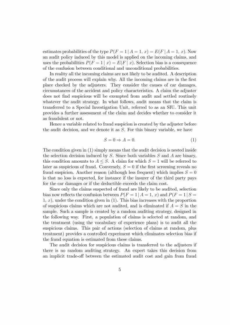
detection. Most of the suspicious claims are not audited if the audit decisionis left to the experts (see for instance Section 3).To sum up, Figure 1 describes the links between the three binary variables

S, A and F , depending on the audit strategy.

Figure 1: The binary variables S, A and F and audit strategies

Random auditingstrategy (A = S)

Incoming claim

A=S=0 A=S=1AAAA

¡¡

¡¡

AAAA

¡¡

¡¡

F=0 F=1

Usual auditingstrategy (A ≤ S)

Incoming claim

@@@@

¡¡

¡¡

S=1S=0

¢¢¢¢

A=0 A=0 A=1AAAA

¡¡

¡¡

AAAA

¡¡

¡¡

F=0 F=1

6

3 Presentation of the data base

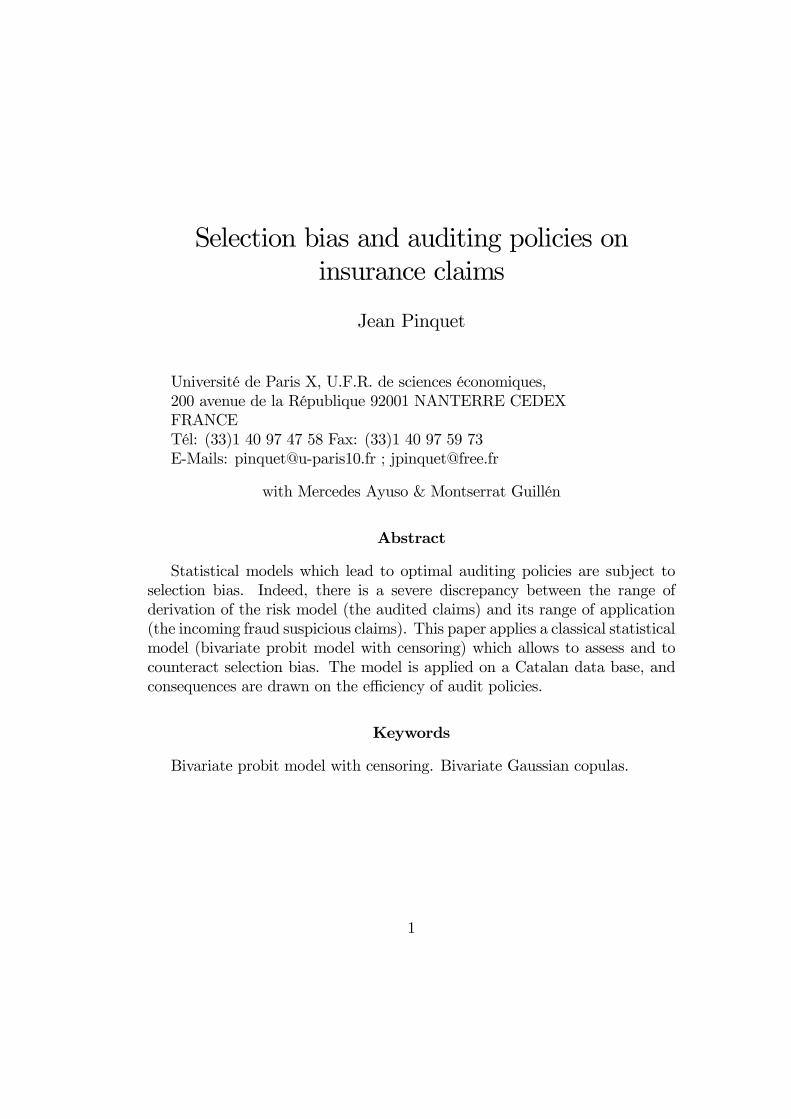
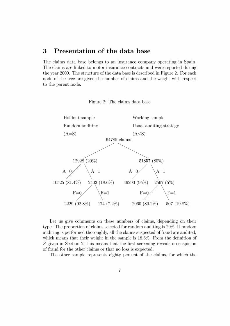
The claims data base belongs to an insurance company operating in Spain.The claims are linked to motor insurance contracts and were reported duringthe year 2000. The structure of the data base is described in Figure 2. For eachnode of the tree are given the number of claims and the weight with respectto the parent node.

Figure 2: The claims data base

Working sample

Usual auditing strategy

(A≤S)

Holdout sample

Random auditing

(A=S)64785 claims

HHHHHHHH

©©©©©©©©12928 (20%)

AAAA

¡¡

¡¡

51857 (80%)

A=0 A=1 A=0 A=1AAAA

¡¡

¡¡

10525 (81.4%) 2403 (18.6%)AAAA

¡¡

¡¡

49290 (95%) 2567 (5%)AAAA

¡¡

¡¡

F=0 F=1

2229 (92.8%) 174 (7.2%)

F=0 F=1

2060 (80.2%) 507 (19.8%)

Let us give comments on these numbers of claims, depending on theirtype. The proportion of claims selected for random auditing is 20%. If randomauditing is performed thoroughly, all the claims suspected of fraud are audited,which means that their weight in the sample is 18.6%. From the definition ofS given in Section 2, this means that the first screening reveals no suspicionof fraud for the other claims or that no loss is expected.The other sample represents eighty percent of the claims, for which the

7

audit decision is left to the adjusters. The audit rate in this sample is close tofive percent, which is much less than for the first sample of claims selected atrandom. The two samples have the same structure, which means that most ofthe suspicious claims are exempted from audit if the adjusters are left free totake the audit decision. The selection bias issue arises from the discrepancybetween these two rates.As indicated in the introduction, we will use the 51857 claims with no spe-

cific audit recommendation as the working sample, since they are subject toselection bias and are processed in a way currently used by insurance compa-nies. The claims selected at random will be used as a holdout sample in orderto assess the efficiency of the statistical model.The fraud rate on audited claims is 19.8% in the working sample. The

application to the hold-out sample of an estimated fraud equation estimatedon the working sample does not modify the average fraud probability, whichremains close to twenty percent. On the other hand, the similar fraud ratefor the hold out sample is equal to 7.2%. Here we have an example of theoverestimation induced by selection bias and mentioned in the introduction.A single equation model on fraud is unable to even partially fill the gap betweenthe two fraud rates. Determining to what extent a selection model applied tothe working sample can fill this gap is the purpose of the statistical analysiswhich follows.

4 The bivariate probit model: Theory and ap-plications to selection bias assessment

4.1 The theoretical model

Using the notations from Section 2, we define the bivariate probit model on asample of claims suspected of fraud. Referring to Figure 1, the bivariate modeldescribed below corresponds to the right part (S = 1) of the tree associatedwith a usual auditing strategy.A bivariate model on the audit and fraud equation with a joint distribution

on the two random components will be able to assess a fraud probability con-ditioned by the individual characteristics of the claims, but also by the auditvariable A. Once this estimation is carried out, we have a fraud probabilityfor suspicious claims which is unconditional with respect to an audit decisionand which can be used in an optimal audit policy.

8

The bivariate probit model with censoring includes, first of all, an auditequation defined on all the claims which are suspected of fraud. This equationis defined in the following way

Ai = 1[A∗i≥0]; A∗i = (xA)i βA + (εA)i ; (εA)i ∼ N (0, 1) . (2)

The binary variableA is the sign indicator of a latent variable A∗. The varianceof the random variable (εA)i can be set equal to one without loss of generalitybecause of the invariance of A with respect to a multiplication of A∗ by apositive constant. The regression components in the linear equation can bedefined on the policy to which the claim is related or can be claim-specific.They are represented by a line vector whereas the parameters are stacked in acolumn vector which enables a cross product.The fraud equation is defined on the audited claims only. We then write

If Ai = 1 : Fi = 1[F∗i ≥0]; F∗i = (xF )i βF + (εF )i . (3)

The random variable (εF )i also follows a standard normal distribution.If we retain a bivariate normal distribution for ((εA)i , (εF )i), i.e.µ

(εA)i(εF )i

¶∼ N2

µµ00

¶,

µ1 ρρ 1

¶¶ρ ∈ [−1, 1], (4)

we obtain a bivariate probit model. The sign of the correlation coefficient ρ isof paramount importance for the estimation of fraud risk conditional on theaudit variable.In this censored setting, three levels are possible for the dependent vari-

ables. Let us compute the corresponding probabilities. We suppress the indi-vidual index for sake of simplicity.

1. If the claim is not audited, the fraud variable is not observed. We thenhave

P [A = 0] = P [εA < −xAβA] = Φ(−xAβA) = 1− Φ(xAβA), (5)

where Φ is the distribution function of a standard normal variable and

Φ(xAβA) = pA = P [A = 1] = E(A).

The last equality in (5) results from the symmetry in the distributionof εA. The bivariate model is estimated on the suspicious claims only,hence the probability P [A = 0] would be described as P [A = 0 |S = 1]if expressed on all the incoming claims as we did in Section 2.

9

2. If the claim is audited and if fraud is established, we can write

P [A = 1, F = 1 ] = P [εA ≥ −xAβA, εF ≥ −xFβF ]= P [εA ≤ xAβA, εF ≤ xFβF ] = P [Φ(εA) ≤ Φ(xAβA), Φ(εF ) ≤ Φ(xFβF )] .

We again used symmetry in the distribution of the random components.The variables Φ(εA) and Φ(εF ) follow a uniform distribution on [0, 1] andthe distribution function of (Φ(εA),Φ(εF )) is a Gaussian copula indexedby ρ. If

pF = P [F = 1] = P [Φ(εF ) ≤ Φ(xFβF )] = Φ(xFβF ),

we denote the Gaussian copula in the following way

C(ρ, pA, pF ) = P [Φ(εA) ≤ pA, Φ(εF ) ≤ pF ] = P£εA ≤ Φ−1(pA), εF ≤ Φ−1(pF )

¤.

This copula relates a bivariate Gaussian distribution function to its mar-ginal components. Hence the probability of interest is equal to

P [A = 1, F = 1] = C(ρ, pA, pF ). (6)

3. The probability of the last level (claim audited but not fraudulent) is thecomplementary value

P [A = 1, F = 0] = P [A = 1]− P [A = 1, F = 1] = pA − C(ρ, pA, pF ).

Maximizing the log-likelihood on the sample requires a computation of theGaussian copula and of its partial derivatives with respect to the parameters.This function does not have a closed form with respect to Φ and Φ−1 unless ρis equal to the critical values −1, 0 and 1. It can be approximated by Gaussianquadratures (see Dionne, Gagné, Vanasse (1998) for an application to paneldata with endogenous attrition).We now present applications of the model to fraud probability prediction.Under the null hypothesis ρ = 0, fraud probability does not depend on the

audit variable and we have

pF = P [F = 1] = P [F = 1 | A = 1]. (7)

Under the alternative assumption ρ 6= 0, selection bias arises because in thatcase

P [F = 1 | A = 1] = C(ρ, pA, pF )

pA6= pF . (8)

10

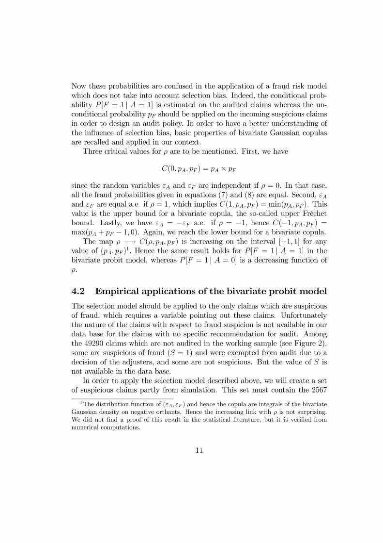
Now these probabilities are confused in the application of a fraud risk modelwhich does not take into account selection bias. Indeed, the conditional prob-ability P [F = 1 | A = 1] is estimated on the audited claims whereas the un-conditional probability pF should be applied on the incoming suspicious claimsin order to design an audit policy. In order to have a better understanding ofthe influence of selection bias, basic properties of bivariate Gaussian copulasare recalled and applied in our context.Three critical values for ρ are to be mentioned. First, we have

C(0, pA, pF ) = pA × pF

since the random variables εA and εF are independent if ρ = 0. In that case,all the fraud probabilities given in equations (7) and (8) are equal. Second, εAand εF are equal a.e. if ρ = 1, which implies C(1, pA, pF ) = min(pA, pF ). Thisvalue is the upper bound for a bivariate copula, the so-called upper Fréchetbound. Lastly, we have εA = −εF a.e. if ρ = −1, hence C(−1, pA, pF ) =max(pA + pF − 1, 0). Again, we reach the lower bound for a bivariate copula.The map ρ −→ C(ρ, pA, pF ) is increasing on the interval [−1, 1] for any

value of (pA, pF )1. Hence the same result holds for P [F = 1 | A = 1] in thebivariate probit model, whereas P [F = 1 | A = 0] is a decreasing function ofρ.

4.2 Empirical applications of the bivariate probit model

The selection model should be applied to the only claims which are suspiciousof fraud, which requires a variable pointing out these claims. Unfortunatelythe nature of the claims with respect to fraud suspicion is not available in ourdata base for the claims with no specific recommendation for audit. Amongthe 49290 claims which are not audited in the working sample (see Figure 2),some are suspicious of fraud (S = 1) and were exempted from audit due to adecision of the adjusters, and some are not suspicious. But the value of S isnot available in the data base.In order to apply the selection model described above, we will create a set

of suspicious claims partly from simulation. This set must contain the 2567

1The distribution function of (εA, εF ) and hence the copula are integrals of the bivariateGaussian density on negative orthants. Hence the increasing link with ρ is not surprising.We did not find a proof of this result in the statistical literature, but it is verified fromnumerical computations.

11

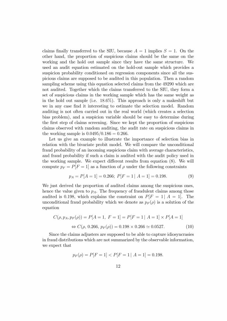
claims finally transferred to the SIU, because A = 1 implies S = 1. On theother hand, the proportion of suspicious claims should be the same on theworking and the hold out sample since they have the same structure. Weused an audit equation estimated on the hold-out sample which provides asuspicion probability conditioned on regression components since all the sus-picious claims are supposed to be audited in this population. Then a randomsampling scheme using this equation selected claims from the 49290 which arenot audited. Together which the claims transferred to the SIU, they form aset of suspicious claims in the working sample which has the same weight asin the hold out sample (i.e. 18.6%). This approach is only a makeshift butwe in any case find it interesting to estimate the selection model. Randomauditing is not often carried out in the real world (which creates a selectionbias problem), and a suspicion variable should be easy to determine duringthe first step of claims screening. Since we kept the proportion of suspiciousclaims observed with random auditing, the audit rate on suspicious claims inthe working sample is 0.0495/0.186 = 0.266.Let us give an example to illustrate the importance of selection bias in

relation with the bivariate probit model. We will compare the unconditionalfraud probability of an incoming suspicious claim with average characteristics,and fraud probability if such a claim is audited with the audit policy used inthe working sample. We expect different results from equation (8). We willcompute pF = P [F = 1] as a function of ρ under the following constraints

pA = P [A = 1] = 0.266; P [F = 1 | A = 1] = 0.198. (9)

We just derived the proportion of audited claims among the suspicious ones,hence the value given to pA. The frequency of fraudulent claims among thoseaudited is 0.198, which explains the constraint on P [F = 1 | A = 1]. Theunconditional fraud probability which we denote as pF (ρ) is a solution of theequation

C(ρ, pA, pF (ρ)) = P [A = 1, F = 1] = P [F = 1 | A = 1]× P [A = 1]

⇔ C(ρ, 0.266, pF (ρ)) = 0.198× 0.266 ' 0.0527. (10)

Since the claims adjusters are supposed to be able to capture idiosyncrasiesin fraud distributions which are not summarized by the observable information,we expect that

pF (ρ) = P [F = 1] < P [F = 1 | A = 1] = 0.198.

12

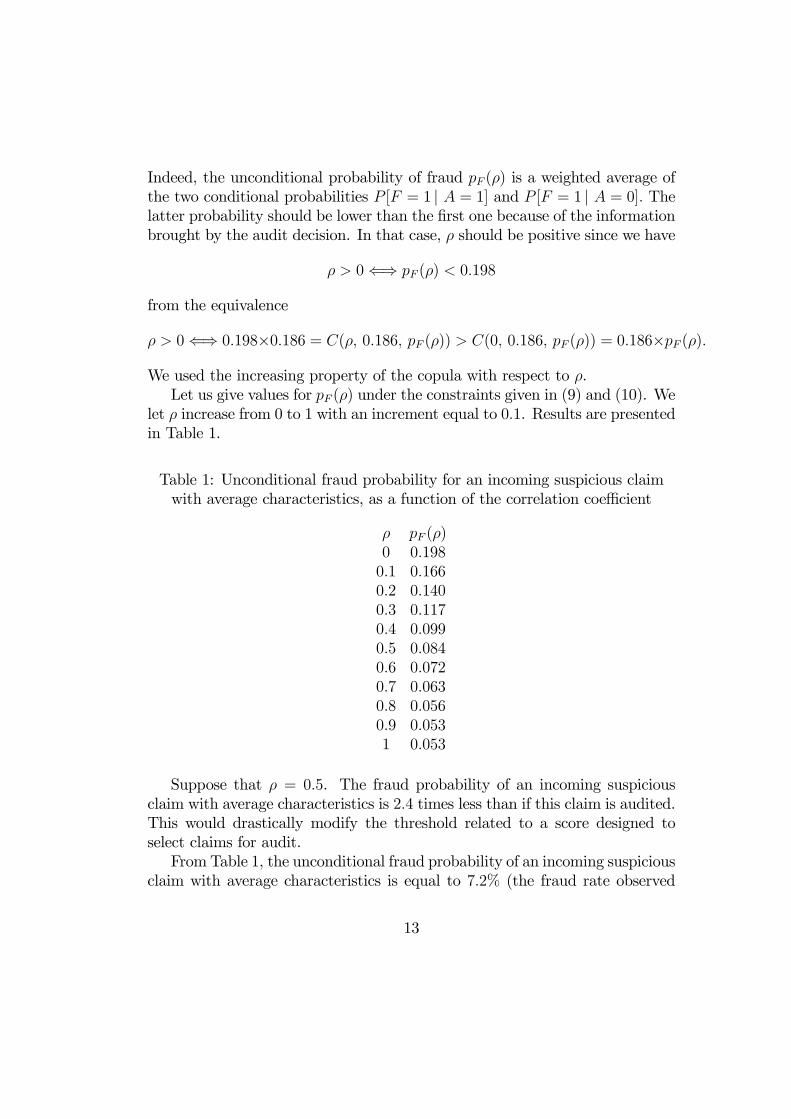
Indeed, the unconditional probability of fraud pF (ρ) is a weighted average ofthe two conditional probabilities P [F = 1 | A = 1] and P [F = 1 | A = 0]. Thelatter probability should be lower than the first one because of the informationbrought by the audit decision. In that case, ρ should be positive since we have

ρ > 0⇐⇒ pF (ρ) < 0.198

from the equivalence

ρ > 0⇐⇒ 0.198×0.186 = C(ρ, 0.186, pF (ρ)) > C(0, 0.186, pF (ρ)) = 0.186×pF (ρ).

We used the increasing property of the copula with respect to ρ.Let us give values for pF (ρ) under the constraints given in (9) and (10). We

let ρ increase from 0 to 1 with an increment equal to 0.1. Results are presentedin Table 1.

Table 1: Unconditional fraud probability for an incoming suspicious claimwith average characteristics, as a function of the correlation coefficient

ρ pF (ρ)0 0.1980.1 0.1660.2 0.1400.3 0.1170.4 0.0990.5 0.0840.6 0.0720.7 0.0630.8 0.0560.9 0.0531 0.053

Suppose that ρ = 0.5. The fraud probability of an incoming suspiciousclaim with average characteristics is 2.4 times less than if this claim is audited.This would drastically modify the threshold related to a score designed toselect claims for audit.FromTable 1, the unconditional fraud probability of an incoming suspicious

claim with average characteristics is equal to 7.2% (the fraud rate observed

13

without selection bias in our data base) for a value of ρ close to 0.6. Hence apositive estimated correlation coefficient is expected on the working sample.This estimated coefficient depends on the choice of regression components

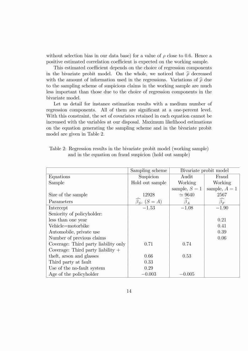
in the bivariate probit model. On the whole, we noticed that bρ decreasedwith the amount of information used in the regressions. Variations of bρ dueto the sampling scheme of suspicious claims in the working sample are muchless important than those due to the choice of regression components in thebivariate model.Let us detail for instance estimation results with a medium number of

regression components. All of them are significant at a one-percent level.With this constraint, the set of covariates retained in each equation cannot beincreased with the variables at our disposal. Maximum likelihood estimationson the equation generating the sampling scheme and in the bivariate probitmodel are given in Table 2.

Table 2: Regression results in the bivariate probit model (working sample)and in the equation on fraud suspicion (hold out sample)

Sampling scheme Bivariate probit modelEquations Suspicion Audit FraudSample Hold out sample Working Working

sample, S = 1 sample, A = 1Size of the sample 12928 ' 9640 2567

Parameters cβS, (S = A) cβA cβFIntercept −1.53 −1.08 −1.90Seniority of policyholder:less than one year 0.21Vehicle=motorbike 0.41Automobile, private use 0.39Number of previous claims 0.06Coverage: Third party liability only 0.71 0.74Coverage: Third party liability +theft, arson and glasses 0.66 0.53Third party at fault 0.33Use of the no-fault system 0.29Age of the policyholder −0.003 −0.005

14

The results depend on the regression components but also on random sam-pling for the bivariate probit model. The estimators are stable with respect tosuspicious claims sampling. With this set of regression components, we have

bρ ' 0.51.Besides, the estimated unconditional fraud probability for incoming suspiciousclaims is 8.4% on average. With this set of regression components, the selectionmodel provides a satisfactory result, since the goal is to reach a 7.2% ratio froma starting point - the fraud rate for audited claims in the working sample -which is 19.8%.As mentioned above, the estimated correlation coefficient increases if fewer

regression components are retained. The estimated coefficient ranges between0.36 and 0.64, depending on the number of regression components. The averageunconditional fraud probabilities range between 6.9% and 10.8%.The positive result obtained in this section is that the selection model is able

to get very close to the actual fraud rate, which can only be reached throughrandom auditing. The weakness of selection models applied to censored datais that estimation results highly depend on the regression components set.

5 Applications of selection bias models to au-diting policies design

An audit decision based on a short term analysis compares estimated audit costand gain from fraud detection. The gain is the product of the claim settlementreserved cost and of the fraud probability2 (see Ayuso, Guillén et al. (2004) forthe inclusion of costs in audit policies). The reserved cost of claim settlementis determined by the adjuster during the first screening of the claim. Henceit is known by the insurance company before the audit decision, which is notthe case with the audit cost. The cost recorded in the data base and relatedto audit corresponds to all the steps of the claim examination, including thefirst screening.Let us denote the audit cost related to the SIU examination for claim i

as aci, and ci the reserved claim cost. A transfer of this claim to the SIU

2If the claim is proved fraudulent, we suppose that the agreement with the policyholderconsists in cancelling the compensation. We discard other possible long-run consequences,such as non-renewal of the policy.

15

generates an expected gain in the short run if

bE [ciFi −ACi] > 0⇔ bE[Fi] = bP [Fi = 1] >bE[ACi]

ci. (11)

Indeed, ci bE[Fi] is the expected gain from audit if claim i is transferredto the SIU. The expected fraud probability is derived from a bivariate probitmodel in what follows. The audit cost is only known ex post (hence its randomvariable status at this step of the computation).Information on audit costs is necessary in order to derive the expected

values bE[ACi]. The average audit costs are given in Table 3 depending on thestatus of the claim and on the sample.

Table 3: Average audit costs (including the first screening)

Average audit costs Hold-out sample Working sampleof claims (A = S) (A 6= S)A = 0 C=36.97 C=37.73A = 1, F = 0 C=59.81 C=67.82A = 1, F = 1 C=231.71 C=222.84

These results clearly indicate that the more a claim is likely to be fraud-ulent, the more it must be examined thoroughly by the adjusters, which in-creases the audit cost. The averages are similar in both samples. The differencebetween the averages of audit costs for claims transferred to the SIU and notfraudulent can be explained by the more severe selection for SIU in the workingsample, which makes these claims more suspicious of fraud. Hence selectionbias also appears for audit costs.The audit costs in Table 3 correspond to all the steps of claims examination,

including the mandatory first screening which is not performed by the SIU.The average audit cost charged to the SIU will be set equal to

acNF = 67.82− 37.73 = C=30.09; acF = 222.84− 37.73 = C=185.11, (12)

where acNF and acF relate to non fraudulent and fraudulent claims. Thiscomputation implicitly supposes that the cost of the first screening does notdepend on the eventual status of the claim.

16

The expected audit cost clearly depends on fraud probability since acF >acNF . Conditioning this expectation on average values for each level of theaudited claims, we obtain

bE[ACi] =³ bP [Fi = 1]× acF

´+³ bP [Fi = 0]× acNF

´= acNF +

³ bP [Fi = 1]× (acF − acNF )´,

An audit policy can be designed from this assessment of the audit cost.The rule given in (11) suggests transfer claim i to the SIU if

ci > acF − acNF & bP [Fi = 1] >acNF

ci − (acF − acNF ). (13)

Since the probability threshold must be less than one, the first conditionamounts to ci > acF . We will use the hold-out sample to compare the au-dit policies derived from different fraud models. All the suspicious claims areaudited if random auditing is performed thoroughly. In that case there is noselection bias and the target audit rate is obtained from a fraud equation esti-mated on the audited claims in the hold-out sample. From the fraud equationspecified in the bivariate model of Table 2, and with the selection rule andthe audit costs given in (13) and (12), we obtain an audit rate for suspiciousclaims of 36.7%.Let us assess the influence of selection bias on audit policies. Suppose that

the fraud equation specified in Table 2 is estimated on the audited claims of theworking sample. The optimal audit rate on suspicious claims of the workingsample goes up to 62%, which reflects the overestimation of fraud probabilityif selection bias is neglected.Let us see how the target audit rate obtained in the first place can be

approximated by a selection model. The proportion of suspicious claims whichshould be audited in the working sample is 39% if we use the selection modelestimated in Table 2. This audit rate is rather close to the target rate obtainedfrom random auditing (i.e. 36.7%), which is a satisfactory result.If the set of regression components varies in the regression, the optimal au-

dit rate ranges between 33 and 45% in our different trials. These rates stronglydepend on the set of regression components through the estimated correlationcoefficient. This result is obviously negative since sound risk assessment de-rived from random auditing cannot be precisely anticipated from the selection

17

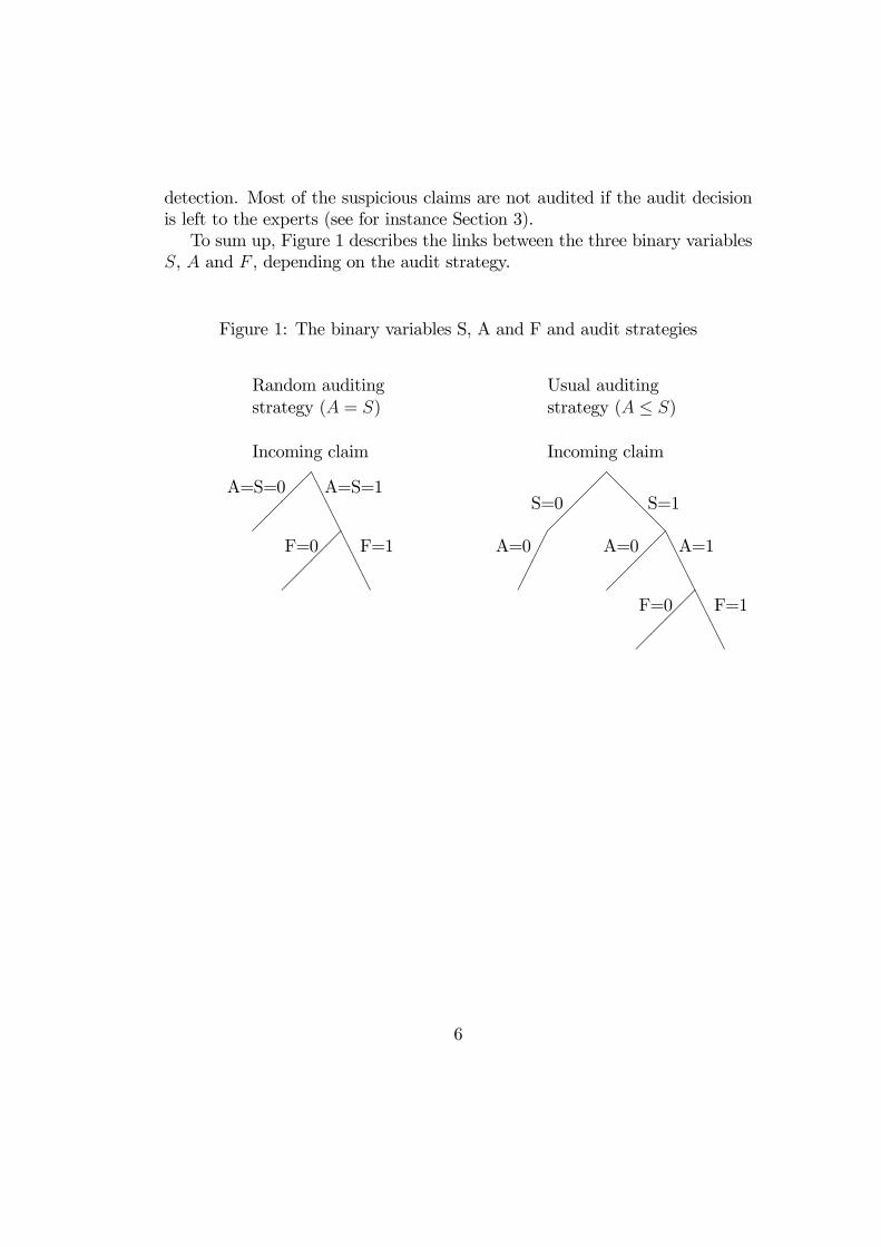
model. However the bivariate probit model points out selection bias and canjustify a random auditing strategy which is not often employed by insurancecompanies.The efficiency of these audit policies is almost the same for all of them,

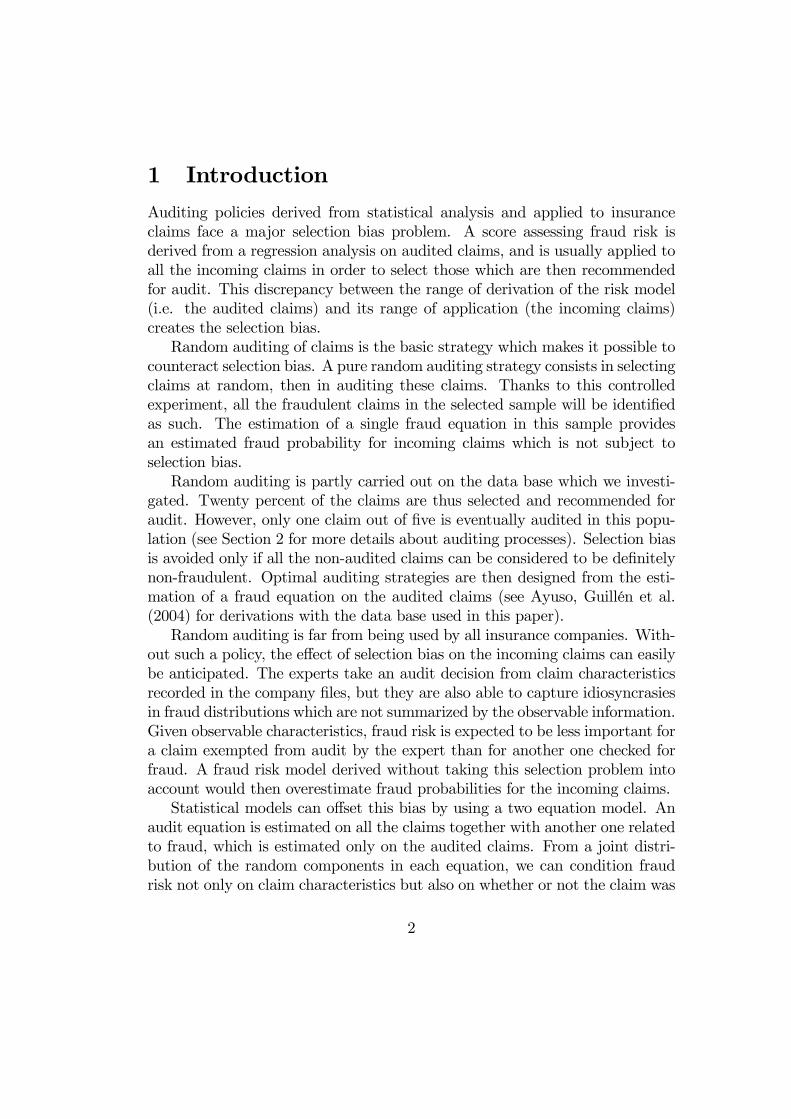
which may seem surprising since the audit rates exhibit great variations. Asfor the selection rule given in (13), we compare these policies to a zero auditstrategy. Hence gains are the reserved costs of the audited claims provedfraudulent in the hold-out sample, and losses are the audit costs charged tothe SIU. For all the preceding audit policies, the average gain per suspiciousclaim is close to C=52. This stability with respect to audit rates is explainedby the shape of efficiency curves. If claims are sorted in decreasing order withrespect to the expected gain bE [ciFi −ACi], the average gain per suspiciousclaim expressed as a function of the audit rate provides such a curve. Figure3 is related to the bivariate model estimated in Table 2.All the efficiency curves have the same shape. This one reaches its maxi-

mum for an audit rate close to 60%. The stability of the curve for audit ratesgreater than 30% explains why the different policies have similar efficiencies.

18

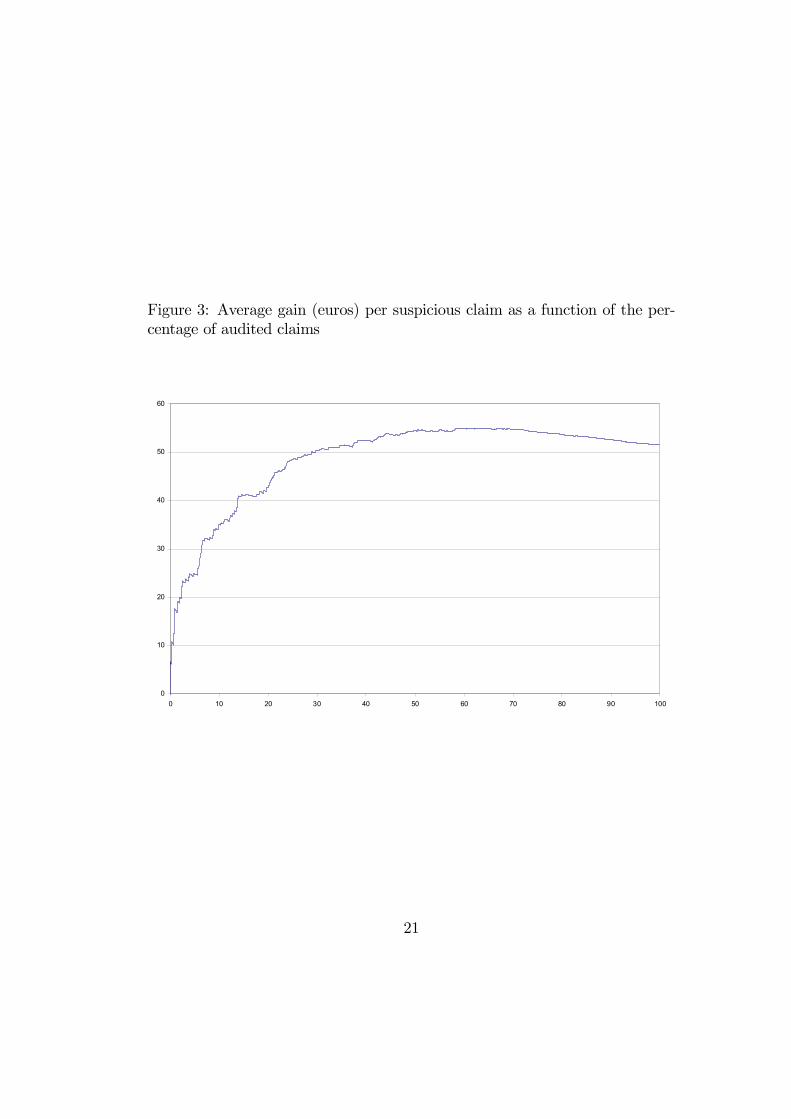
Figure 3: Average gain (euros) per suspicious claim as a function of the per-centage of audited claims

0

10

20

30

40

50

60

0 10 20 30 40 50 60 70 80 90 100

21

6 Conclusions

Let us first comment briefly on the instability of selection bias assessment withrespect to the set of regression components. This instability is actually con-substantial with the censored character of the data. We presented censoredand non-censored selection models in the introduction. Such models are madeup of a selection variable (e.g. audit), a variable of interest (e.g. fraud) andare censored if the variable of interest is observed only on the selected individ-uals. For a non-censored model, the influence of the selection variable on thevariable of interest is easily derived from the comparison of two samples (se-lected versus not selected individuals) with respect to the variable of interest.In a censored context, this influence is only assessed through the variation ofestimated selection probabilities on the selected individuals. This estimatedprobability plays the role of a supplementary covariate in the regression modelrelated to the variable of interest. Now this probability is derived from theinformation already used in the regression. Selection bias reflects a more intri-cate specification for the distribution related to the variable of interest insteadof being based on observed differences in the non-censored setting3. If theselection model is unstable for censored data, it is however of greatest interestprecisely in this context.Since random auditing cannot be avoided in order to obtain a sound as-

sessment of fraud probabilities, we find it interesting to derive the cost ofthis controlled experiment on our data base. The relative costs of the auditstrategies in the two samples described in Figure 2 can be derived with respectto a situation where no claim is transferred to the SIU, which we did in thelast section. Hence gains are the reserved costs of the audited claims provedfraudulent, and losses are the audit costs charged to the SIU.The result is striking. The controlled experiment (i.e. random auditing)

actually generates more gain for the insurance company than the usual auditstrategy, regardless of the possible future gains induced by better fraud prob-ability assessment. Hence the insurance company would probably have savedmoney had all the suspicious claims of the working sample been transferred tothe SIU. In addition, increasing the audit rate reduces fraud risk because ofthe deterrence effect of audit policies (see Tennyson and Salsas (2002); Dionne,

3The seminal paper on selection models with censoring is entitled "sample selection biasas a specification error" (Heckman, (1979)). Estimated selection probability is included ina linear regression on the variable of interest via the inverse Mills’ ratio, which creates theso-called "Heckit".

22

Giuliano and Picard (2002)).Lastly, let us mention other issues which must be considered in the design

of an optimal audit policy. First, the anticipation of audit costs could easily beimproved since our analysis remained at a basic level. More important is theimpact of claims settlement decisions on the policyholder’s value. The thor-ough audit of a claim may modify the relationship between the policyholderand the insurance company. If the claim is not found to be fraudulent, theinsured may take the audit process amiss and the attrition rate should riseas a consequence. If the claim is found fraudulent, the risk level of the poli-cyholder will be updated at a higher level. A fraud event usually triggers anincrease in premium or a cancellation of the policy. Taking into account thepolicyholder’s value in an audit decision would increase both gains and lossescomputed in the short run in Section 5. This would also imply a long-runeconometric analysis from the policies data base.

References

[1] Artis, M., M. Ayuso and M. Guillén, 2002, Detection of Automobile In-surance Fraud with Discrete Choice Models and Missclassified Claims,Journal of Risk and Insurance, 69(3): 325-340.

[2] Ayuso, M., M. Guillén, S. Viaene, and D. Van Ghee, 2004, Cost-SensitiveDesign of Claim Fraud Screens, Lecture Notes in Artificial Intelligence,3275, 78-87.

[3] Belhadji, E.B., G. Dionne and F. Tarkani, 2000, AModel for the Detectionof Fraud, Geneva Papers on Risk and Insurance - Issues and Practice,25(5): 517-538.

[4] Chiappori, P.A. and B. Salanié, 2000, Testing for Asymmetric Informationin Insurance Markets, Journal of Political Economy, 108(1): 56-78.

[5] Dionne, G., R. Gagné and C. Vanasse, 1998, Inferring Technological Pa-rameters from Incomplete Panel Data, Journal of Econometrics, 87: 303-327.

[6] Dionne, G., F. Giuliano and P. Picard, 2002, Optimal au-diting for insurance fraud, Working paper, available athttp://www.hec.ca/gestiondesrisques/cahiers.htm .

23

[7] Hand, D.J. and W.E. Henley, 1997, Statistical Classification Methodsin Consumer Credit Scoring: A Review, Journal of the Royal StatisticalSociety A, 160: 523-541.

[8] Hausman, J.A. and D.A. Wise, 1979, Attrition Bias in Experimental andPanel Data: The Gary Income Maintenance Experiment, Econometrica,47(2): 455-474.

[9] Heckman, J.J., 1979, Sample Selection Bias as a Specification Error,Econometrica, 47(1): 153-162.

[10] Heckman, J.J., 2000, Microdata, Heterogeneity and the Evaluationof Public Policy, Nobel Prize Lecture, available on the Web sitehttp://nobelprize.org/.

[11] Rosenbaum, P.R. and D.B. Rubin, 1983, The Central Role of the Propen-sity Score in Observational Studies for Causal Effects, Biometrika, 70:41-55.

[12] Tennyson, S. and P. Salsas-Forn, 2002, Claims Auditing in AutomobileInsurance: Fraud Detection and Deterrence Objectives, Journal of Riskand Insurance, 69( 3): 289-308.

24