SELECTING A FLEXIBLE MANUFACTURING …pure.iiasa.ac.at/3495/1/RR-91-20.pdfSELECTING A FLEXIBLE MANUFACTURING SYSTEM USING MULTIPLE CRITERIA ... such relevant performance criteria as

SELECTING A FLEXIBLE MANUFACTURING SYSTEM USING MULTIPLE CRITERIA ANALYSIS

Antonie Stam Dept. of Management Sciences and Information Technology University of Georgia, Athens, GA, USA

Markku Kuula Helsinki School of Economics Helsinki, Finland

RR-91-20 December 1991

Preprinted from International Journal of Production Research, 1991, Volume 29 , No. 4, 803-820.

INTERNATIONAL INSTITUTE FOR APPLIED SYSTEMS ANALYSIS Laxenburg, Austria

Research Reports, which record research conducted at IIASA, are independently reviewed before publication. However, the views and opinions they express are not necessarily those of the Institute or the National Member Organizations that support it.

Preprinted with permission from International Journal of Production Research, 1991, Vol. 29, No. 4, 803-820. Copyright ©1991 Taylor & Francis Ltd.

All rights reserved. No part of this publication may be reproduced or transmitted in any form or by any means, electronic or mechanical, including photocopy, recording, or any information storage or retrieval system, without permission in writing from the copyright holder.

Printed by Novographic, Vienna, Austria

Preface

A visual interactive decision support framework based on a multiobjective programming model designed to aid the decision-maker, typically top management, in selecting the most appropriate technology and design when planning a flexible manufacturing system (FMS) is described. The insights gained from experimenting with the different scenarios form the basis of understanding the anticipated impact of techno-economic factors on the performance of the FMS configuration, and provide valuable information for the implementation stage of building the FMS. An example using real data from a case study in the Finnish metal product industry is provided to illustrate the methodology. Most of the work was carried out while the authors were visiting the SDS Program at IIASA and it provides a good example of applied methodological research in Decision Support Systems.

ALEXANDER KURZHANSKI Leader

System and Decision Sciences Program

lll

INT. J. PROD. RES., 1991 , VOL. 29, NO. 4, 803- 820

Selecting a flexible manufacturing system using multiple criteria analysis

ANTONIE STAMt and MARKKU KUULAt

A visual interactive decision support framework designed to aid the decision-maker, typically top management, in selecting the most appropriate technology and design when planning a flexible manufacturing system (FMS) is described. The framework can be used in the preinvestment stage of the planning process, after the decision in principle has been made to build an FMS. First, both qualitative and quantitative criteria are used to narrow the set of alternative system configurations under consideration down to a small number of most attractive candidates. After this prescreening phase, a multiobjective programming model is formulated for each remaining configuration, allowing the manager to explore and evaluate the costs and benefits of various different scenarios for each configuration separately by experimenting with different levels of batch sizes and production volumes. The system uses visual interaction with the decision-maker, graphically displaying the relevant trade-offs between such relevant performance criteria as investment and production costs, manufacturing flexibility, production volume and investment risk, for each scenario. Additional criteria, when relevant, can also be included. The ease of use and interpretation and the flexibility make the proposed system a powerful analytical tool in the initial FMS design process. The insights gained from experimenting with the different scenarios form the basis of understanding the anticipated impact of techno-economic factors on the performance of the FMS configuration, and provide valuable information for the implementation stage of building the FMS. An example using real data from a case study in the Finnish metal product industry is provided to illustrate the methodology.

1. Introduction Many companies seek to maintain or gain a competitive edge in the market-place

by exploiting the advantages of modern manufacturing technologies. One such technology which has become increasingly popular over the past decade is that of flexible manufacturing systems (FMS) (Buzacott and Yao 1986, Jaikumar 1986, Meredith 1987a, b, Ranta et al. 1988). The primary goal of implementing an FMS is to make the production process as versatile or flexible as possible in terms of, among other things, an ability to produce a variety of products of different degrees of complexity, short delivery times, easily changed production volumes and batch sizes, and flexible production scheduling (Ranta 1989, Whitney 1985). A higher flexibility in general will enable the company to adjust more easily to changes in the market-place and customer needs, while maintaining high quality standards for the products. Prior to implementing an FMS, however, a careful feasibility and performance analysis is needed in which the impacts of various technological, economic, design, managerial and social factors associated with the FMS are considered. Recent studies have shown that the most

Revision received July 1990. t Department of Management Sciences and Information Technology, College of Business

Administration, University of Georgia, Athens, GA 30602, USA. t Helsinki School of Economics, Runeberginkatu 14-16, SF-00100 Helsinki, Finland.

0020-7543/91 $3-00 © 1991 Taylor & Francis Ltd .

804 A. Stam and M . Kuula

important of these factors are related to the design, implementation, social and managerial aspects of the FMS, rather than the technology itself (Ranta 1989, p. 2). Thus, the FMS selection problem is a strategic question which typically has to be decided by top-level management (Choobineh 1986, Wabalickis 1988, Ranta 1989).

In most situations, a number of alternative FMS configurations are available. Given the strategic nature of the FMS investment, the question is how to analyse effectively which of the feasible configurations is the most appropriate. Two widely used approaches to analyse the performance of FMS configurations are simulation studies and studies using analytical models. Buzacott and Yao (1986) in their review article of FMS note that 'while simulation models are of great value for evaluating specific systems designs, analytical models are superior in terms of the amount of insight which they give' (p. 902). Moreover, they conclude their paper by stating that ' .. . due to their complexity, the new manufacturing systems now being developed are only partly understood from a system perspective (Gershwin et al. 1984) . . .' so that ' ... analytical models can provide the necessary insights'.

This present model belongs to the category of analytical models. We present here a decision support framework which can aid the decision-maker (top-level management) in the preinvestment stage of designing the most suitable FMS. The main contribution of this paper is to provide a structured framework to support management's general understanding of the dynamics of the decision problem at hand and, specifically, to assist management in selecting the 'most appropriate' FMS design from a set of available candidate configurations, through extensive scenario analysis and evaluation of the trade-offs between the various decision criteria. Of course our framework does not comprehensively cover the scope of the complex overall decision of acquiring an FMS. Therefore, the decision-maker should use our decision support system in conjunction with other complementary types of analysis, such as a financial feasibility study and a study of the organizational impacts (retraining workers, new structures, etc.) of the FMS conversion.

Our decision support framework consists of two phases. In the initial prescreening phase, the executive support system 'Expert Choice' (Forman and Saaty 1987) is used to narrow the usually relatively large group of candidate configurations down to the three or four 'most attractive' configurations. A nice feature of this software package is that it allows for both qualitative and quantitative factors and criteria to be considered. The remaining three or four candidate configurations are then analysed further in more detail in the second phase. The analysis in phase two is quantitative and involves solving a multiobjective mathematical programming formulation of the problem in which, for each configuration, various scenarios are explored interactively. The decision-maker evaluates the trade-offs between relevant decision criteria, such as production volume, investment costs and flexibility, by varying the batch size and production volume of each part and controlling the utilization of the machines. The VIG package (Korhonen 1987) was selected for this analysis because its graphical displays and user-friendly interaction between decision-maker and model make it well suited for analysing the type of problem under consideration here.

The remainder of the paper is organized as follows. First, the general decision support system methodology and the multiobjective programming formulation are introduced, with a detailed discussion of the different components related to costs and flexibility. Next, a specific application of the decision support system to a Finnish metal product firm is described, followed by an exposition of how the decision support system can be used in practice. The paper is concluded with final remarks.

Selecting a flexible manufacturing system 805

2. DSS framework As mentioned previously, the proposed methodology consists of two phases. In

each phase, specialized analytical tools with a high-power user interface are used to analyse the pertinent questions. It is assumed that, prior to using the decision support system, initial data have been collected and a preliminary study has been performed to identify and globally characterize the set of all candidate design configurations for the FMS. A general description of the two phases is given below.

2.1. Phase 1 The initial number of available alternatives may be relatively large and, therefore,

difficult to manage in terms of evaluating the trade-offs. Research has found that the human mind can effectively evaluate trade-offs between, at most, five to seven alternatives simultaneously (Steuer 1986). The personal experience of one of the authors with decision-makers in previous interactive computer applications involving multiple criteria confirms this finding (Stam et al. 1987). For this reason, a prescreening procedure is applied in phase 1 to narrow down the list of candidate FMS configurations to a more manageable number. Depending on the specific application, a reasonable number appears to be three or four alternatives, but in some situations many attractive alternatives may exist, whereas in other cases only a few viable configurations are available. The commercially available package 'Expert Choice' (Forman and Saaty 1987) allows for the analysis of trade-offs related to quantitative criteria such as costs, as well as qualitative criteria such as organizational and social impacts of the FMS design. Thus, a useful aspect of the prescreening analysis is that all FMS design configurations can be evaluated simultaneously on both 'hard', or tangible criteria which can be expressed numerically, and 'soft', or intangible, criteria which cannot meaningfully be expressed in terms of numbers (Arbel and Seidmann 1984). Other packages which can be used to analyse discrete alternative multicriteria problems with quantitative as well as qualitative criteria are DISCRET (Majchrazak 1988), developed in Poland in conjunction with the International Institute for Applied Systems Analysis (IIASA) in Austria and AIM (Lotti 1991). DISCRET is based on the reference-point method developed by Wierzbicki and Lewandowski (Lewandowski and Wierzbicki 1988; Wierzbicki 1979, 1982). AIM is based on aspiration-level decision making.

Expert Choice is quite powerful and has been used in numerous real applications (Saaty 1987, Forman and Saaty 1987, Dyer et al. 1988) and executive decision situations. The theoretical foundation of Expert Choice is based on the analytic hierarchy process (AHP) developed by Saaty (1980, 1987). This approach has recently been recommended by Wabalickis (1988) as a useful methodology for justifying an FMS. However, Wabalickis did not use the Expert Choice software, but his own calculations and computer programs to calculate the results, and his approach was quite limited and not interactive, in contrast to our approach (using Expert Choice) which is both interactive and on-line, and flexible in the way in which the decisionmaker prefers to provide the necessary information. Arbel and Seidmann (1984) have reported a successful real industrial application using the AHP for FMS selection.

The main idea behind the modelling philosophy of Expert Choice is to divide the decision problem into smaller subproblems, making it easier for the decision-maker to evaluate trade-offs. For instance, a global criterion such as FMS investment and production costs can be subdivided into several subcriteria such as software costs, tool costs and training costs. These subcriteria can in turn be refined further, creating a

806 A. Stam and M. Kuula

hierarchical tree structure of the decision problem. The lowest level of this tree contains the alternatives (in our application the different possible FMS configurations).

The manager can evaluate these alternatives in two different ways. One way is to make pairwise comparisons, first between each of the global criteria at the highest level of the hierarchy, making judgements on their relative importance, followed by comparisons of the lower level criteria. Finally, the alternatives are compared pairwise according to their importance with respect to each criterion. The pairwise comparisons are used to calculate a composite importance weight for each of the alternatives, resulting in a final ranking of the alternatives. The alternative with the highest ranking is the 'most preferred' one, given the preference information provided by the decisionmaker through the pairwise comparisons. This approach, however, requires a multitude of pairwise comparisons, and is not feasible if the number of alternatives or criteria is considerable. The other way to evaluate the alternatives is the ratings approach, where the alternatives are directly rated on a scale of 1 to 9 with respect to each of the criteria, after which again the composite ranking score is calculated. This option is particularly useful if the number of alternatives is too large to make all pairwise comparisons. After the ranking process of alternatives has been completed, Expert Choice facilitates extensive graphical and numerical sensitivity analyses where the sensitivity of the ranking to changes in the manager's importance judgements can be tested.

Our use of the final rankings provided by Expert Choice differs slightly from the way in which these are typically used. In most cases, the alternative with the single highest ranking is selected as the 'most preferred' and implemented. In our approach, however, the Expert Choice analysis is only a prescreening phase where undesirable and Jess attractive alternatives are eliminated from further consideration. Therefore, rather than one alternative, a small group of alternative candidate configurations is selected for the analysis in the second phase.

2.2. Phase 2 Phase 2 differs from phase 1 in several ways. First, in the prescreening phase only

general judgements about the level of each criterion are required, while in the second phase detailed quantitative information is needed. For instance, in the prescreening process the investment costs can be described in terms of categories such as 'very high', 'high', 'average' and 'low', while in phase 2 numerical (ratio scale) values are used and the trade-offs between the criteria are of a quantitative nature. Second, only a small number of alternatives remain and are analysed in more detail using quantitative techniques. Third, in the second phase the methodology seeks to explore the performance trade-offs between the relevant criteria of each remaining FMS configuration, subject to the physical limitations and performance characteristics of the design. This analysis requires formulating the relevant aspects of each FMS configuration in terms of a multiobjective mathematical programming problem. A separate model should be formulated for each configuration, because each has its own unique specifications. It should be noted that Expert Choice does not have the ability to deal with this type of multiobjective decision model.

In the formulation, the operational decision variables include the quantity of each part to be produced and the batch size of each part. The constraints include physical limits to the amount of time available on each machine. As alluded to above, the criteria include the costs associated with acquiring the FMS configuration, the total production volume of each member of the part family, and the degree offlexibility of the


configuration. The previously determined configuration-specific parameter coefficients are used as input for the formulation. It is very important that the input parameters are reasonably accurate, because the results of the multiobjective analysis can be sensitive to the values of these coefficients.

After considering a number of different multicriteria software packages, the visual interactive goal programming (VIG) package (Korhonen 1987) was selected for the analysis in phase 2, mainly because of its attractive graphical user interface. The method allows the decision-maker to move freely on the Pareto optimal surface. The user can search the set of efficient solutions by controlling the speed and the direction of the motion (Korhonen and Soismaa 1988). A solution is said to be Pareto optimal or efficient if none of the criteria can be improved without sacrificing at least one of the other criteria. Thus, the decision-maker can be confident that inferior solutions are automatically eliminated, and only relevant solutions will be considered throughout the interactive decision process. Thus, at any time during the interactive process, the decision-maker has on-line control over the decision parameters (batch size and production volume of each member of the part family), controls the target utilization rates of the machines, and can directly observe the changes in the criterion values and the associated trade-offs between criteria on the screen in the form of easily interpreted bar graphs. The mathematical details of VIG can be found in Korhonen and Laakso (1986). Korhonen and Wallenius (1988) have described an implementation of the method.

3. Multiobjective formulation The two major critical resources in modelling the FMS decision are, on the one

hand, the capital needed for the FMS investment, which largely depends on the costs of the FMS configuration, and, on the other hand, time, as each machine can operate only for a limited number of hours annually. The cost and time resources are interrelated and often conflicting parameters. For instance, more time-efficient machines are obviously more expensive, but can provide more efficient tooling times. The nature of these two scarce resources is described below. The model formulation closely follows that described by Ranta and Alabian (1988) and Ranta (1989). 1

Suppose a particular FMS configuration consists of m machines which are to produce n different parts. Define the actual tooling time of part i on machine j by T;i, and the unit overhead time including changing, waiting, checking and repairing by tii. Furthermore, let the batch size and the number of batches produced per period (e.g. annually) of part i be given by b; and V;, respectively, so that the total production volume per period of part i is represented by V; = b;v;, and the total production volume of all parts combined by

n

V= L V; i= 1

3.1. Costs All cost figures are expressed in US dollars. The total costs of the FMS may be

divided into machine costs (CM), tool costs (Cd, parts pallet costs (Cp), software costs (Cs), transportation costs (CT) and other costs (C0 ) . Thus, total costs C can be represented as

C=CM+CL +Cp+Cs+CT+Co (1)

1 After contacting the authors of the original case study, some of the original data were found to be incorrect. The data used in our paper are the corrected values.


Each of these cost components is explained below. Assuming that only the direct investment costs are included in the machine costs, CM can be written as

m

CM= L eiMi j=l

(2)

where Mi is the direct investment cost of machine j in dollar minutes per millimetre, and ei is the relative efficiency of machinej, which can be expressed in terms of the time needed for the machining of one unit of part i on machine j (T;i + tii) and the total production volume of the parts, b;v;, weighed by the coefficient e;i which represents the relative efficiency of machine j on part i. Thus, ei is given by

n

ei= L eiib;v,{T;i+tii)/TiMAX (j= 1, ... ,m) (3) i= 1

The tool costs CL depend on the complexity of the parts and the number of tools needed

n n m

CL= L qg;9;+ L L qjiij• (4) i=l i=lj=l

where 9; is the complexity of part i as measured by the form of the part, precision and other factors, and l;i is the number of tools needed to produce part ion machine j, while q9; and qii are appropriate estimates of the per unit dollar contributions to tool costs.

The parts pallet costs depend on part complexity, batch size and the number of batches produced per period of each part:

n n n

Cp = L P9;9; + L Pb;b; + L PmV; (5) i=l i=l i=l

where p9;, Pb; and Pvi are part-dependent per unit contribution factors. Empirical studies have shown that software costs are related to numerical control

(NC) programs, scheduling and communication algorithms, and to the number of interfaces needed (Ranta 1989). Thus it is reasonable to write the software costs Cs as follows:

n n n m m

Cs= L s9 ; + L (s + Sv;)V; + L L h;iij + L Sejej (6) i=l i=l i=lj=l j=l

where the first term is related to software complexity, the second to the number of batches produced per period, the third to tool management, and the fourth to machine efficiency. The terms s, s9i, svi• hii and sei are per unit cost coefficients.

The internal transportation costs CT include costs associated with transportation devices and storage:

n n

CT=uV+ Luigi+ L uvivi (7) i= 1 i= 1

which depends on the capacity of the system V, the complexity of the parts 9i and the number of batches vi. The coefficients u, ui and uvi are scalar multipliers.

Finally, the remaining costs are represented by the category of other costs (C0 ):

Co= CTR + CREs (8)

C0 includes personnel training costs (CTR= cPLP L, where PL is the hours of training needed) and residual costs (CRES). These costs do not depend on the decision variables (batch size and production volume of the parts).


3.2. Time The second scarce resource is machine time (all times are in minutes). The total time

machine j is used during the period is given by ~ n

~= L (~j+ tij)b;V; (j=l, ... ,m) (9) i= 1

where the parameters are as defined above. The technical non-availability (idle) time or machine disturbance time of machine j (Id) depends on part complexity and the number of batches of each part type, on the size and complexity of the software needed (S) and a personnel training factor. Thus, Idi can be expressed as

n n

Idi= L df/J;+ L dtiv;+djSi-dfLPL (j= 1, ... ,m) (10) i= 1 i= 1

The coefficients dfi, dti, dj and dfL are positive scaling constants representing the per unit disturbance time in minutes. The disturbance formula (eqn. (10)) has an empirical basis (Ranta 1989, p. 15), and has been confirmed by .several recent case studies (Kuivanen et al. 1988, Lakso 1988, Norros et al. 1988).

Denoting the maximum theoretical number of minutes which machine j can operate per time period by J;"MAX• then using the utilized time(~) and non-available time (Jdi) of machine j, the following expression holds:

~ + 1dj ~ 7;"MAX (j=l, ... ,m) ( 11)

Since the left-hand side of eqn. (11) is a measure of the utilization ofmachinej, we can impose a minimally acceptable utilization J;"MtN• so that eqn. (11) becomes

J;"MIN ~ ~ + Jdj ~ i;"MAX (j=l, ... ,m)

Aggregating eqn. (12) over all machines we derive the systems level constraint

TMIN ~ T + Td ~ TMAX

(12)

(13)

where TMIN is the minimally acceptable utilization of the system, TMAX is the physical upper bound on the utilization time of all m machines,

m

T=I ~ j= 1

is the total utilized time of all m machines combined, and m

14= I 7dj j= 1

is the total machine disturbance time. Note that while usually m

TMAX = L i;"MAX j=l

holds, as it represents a physical limitation to the system, it is not necessarily true that m

TMIN = L J;"MIN• j= I

because the appropriate value of this parameter is set by management.


3.3. Objectives The general problem of the FMS design is to maximize the production volume

within the system-dependent machine time constraints, while at the same time minimizing the costs and maximizing flexibility by possessing the ability to produce a diverse and complex part family, using as small a batch size as possible. These three important criteria are formulated as

n

maximize PRODUCTION= L bivi (14) i= 1

minimize COST= C (15)

n n n

maximize FLEXIBILITY= L f 9igibivi+ L fvibivi- L fb;b; (16) i=l i=l i=l

The functional form (eqn. (14)) representing total production volume differs from that given by Ranta and Alabian (1988) and Ranta (1989) as in eqn. (14a), where only the number of batches was included:

n

PRODUCTION= L V;. (14a) i= 1

The formulation in eqn. (14) appears more appropriate. The cost function (eqn. (15)) was introduced above (see eqns (1) and (3}-(8)). Flexibility in eqn. (16) is measured as a function of complexity, production volume and batch size, where the minus sign of the third term indicates that smaller batches are preferred, because smaller batches imply a higher degree of flexibility. The coefficients f 9;,fvi and !bi are positive scalar constants, indicating the relative importance of the different measures of flexibility.

Depending on the decision-maker's needs, it is possible to refine and extend these criteria. For instance, one can assign relative importance weights to the production of different members of the part family. This may be appropriate if certain parts yield more valuable final products or realize higher contributions (e.g. as measured by profits) to the firm. Denoting the relative importance of part i by W;, we can replace eqn. (14) by

n

maximize W_PRODUCTION = L w;b;v; (17 a) i= 1

In many cases, however, maximizing a linear combination of the production volumes of individual parts (such as in eqn. (17 a)) may not be appropriate or insightful. If the parts can be grouped into k disjoint more or less homogeneous groups, say G1, ... , Gk> such that G1 u ... uGk={l, ... ,n}, then a useful approach would be to maximize the production volume of each group separately, implying the following set of criteria:

maximize PRODUCTION_l = L b;v; ieG1

(17 b)

maximize PRODUCTION_k = L b;v; ieGk

Using this formulation it is possible to evaluate directly the trade-offs between the production volumes in each group. It is clear that many of the above criteria are conflicting, and that the decision problem of evaluating their trade-offs is a complicated one. In the following section, we illustrate how our interactive decision support system can assist management with this difficult task.


4. Example The example is based on a real case. More specifically, the data were collected by

Ranta (Ranta and Alabian 1988) and are based on a real system in the Finnish metal product industry. For reasons of confidentiality the name of the company is not revealed. A few years ago this company went through a research and development phase in which management conducted a series of interviews to pin-point problems in production. A subsidiary of the company produces gears for diesel engines, and it was decided to consider an FMS for this subsidiary. A section of the subsidiary producing 80 different parts is used to illustrate how our decision support framework can be applied in the FMS predesign stage.

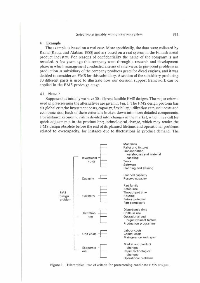
4.1. Phase 1 Suppose that initially we have 30 different feasible FMS designs. The major criteria

used in prescreening the alternatives are given in Fig. 1. The FMS design problem has six global criteria: investment costs, capacity, flexibility, utilization rate, unit costs and economic risk. Each of these criteria is broken down into more detailed components. For instance, economic risk is divided into: changes in the market, which may call for quick adjustments in the product line; technological change, which may render the FMS design obsolete before the end of its planned lifetime; and operational problems related to overcapacity, for instance due to fluctuations in product demand. The

Machines Pallet and fixtures Transportation,

warehouses and material lov~tmoot~ handling costs Tools

Software Planning and training

_c Planned capacity Capacity Reserve capacity

Flo>ibility ·~ Part family Batch size

FMS +- Throughput time design Routing problem Future potential

Part complexity

Disturbance time

uw;,.,100 t Shifts in use rate Operational and

organizational factors Production programme

Unit costs ·-E Labour costs Capital costs Maintenance and repair

Market and product

Eoooomio f changes risk Rapid technological

changes Operational problems

Figure 1. Hierarchical tree of criteria for prescreening candidate FMS designs.


Criteria

Investment costs . . . Economic risk

Pallet and Market Technology Operations Total Alternative Machines fixtures adaptation adjustment (Utilization) rating

1 Medium Medium ... Easy Fast Good 0·302 2 High Low Easy Average Good 0·283 3 High Medium Easy Average Excellent 0·265 4 Very high Medium Average Fast Average 0·212 5 High Very high Easy Average Average 0·196 6 Very high High Average Fast Good 0·166 7 Medium Medium Average Average Good 0·151 8 High High Average Average Poor 0·145 9 High Medium Average Slow Average 0·139

10 Medium Low ... Difficult Fast Average 0·127

Table 1. Partial prescreening ratings of the ten highest scoring FMS designs.

second-level criteria can also be refined, but this is not shown in Fig. 1. Software costs, for example, may relate to NC programs and systems control, communication, scheduling, tool management and diagnostic software.

Each of the criteria shown in Fig. 1 is compared pairwise with the other criteria at the same level and branch, yielding a composite importance weight for each lowest level criterion. All 30 candidate FMS designs are separately rated on these criteria. Higher ratings are better, and each final rating is between zero and one. The evaluations of the alternatives with respect to each of the criteria are provided by the decision-maker. Table 1 shows a representative part of the results from the ratings process for the ten highest ranking alternatives. Note that the categories of evaluation are quite general and qualitative. For instance, alternative 5 is judged as having 'high' machine costs, and an 'average' ability to adjust to changing technology. From Table 1 it is clear that the top three FMS designs were considerably more highly rated than the others. These three configurations were selected for a more detailed analysis in phase 2.

4.2. Phase 2 We illustrate the phase 2 analysis using FMS design alternative 2 from the

prescreening phase. Without loss of generality, we follow Ranta (1989) in selecting a representative group of 13 members from the original part family of 80. The data are the same as those used in the above study. The general model introduced above was simplified to the linear case along the lines suggested by Ranta and Alabian (1988), by solving the multicriteria problem for fixed batch sizes. In reality, of course, batch sizes can freely be changed. Thus, in order to evaluate comprehensively the trade-offs between the criteria, the analysis should be repeated for several different reasonable batch sizes.

The proposed FMS design consists of one turning machine, two machine centres, one grinding machine and automatic transportation and warehouses for system integration. We discuss here the analysis for the case where the batch size for each part is taken to be 5. This batch size is relatively small and, as mentioned above, for a complete analysis of the model dynamics other batch sizes are to be analysed as well.


The form of the constraints and criteria closely follows the general formulation in eqns (1H16). All model parameters were calculated using eqns (1Hl3). The transportation costs were not available in the present case and ·were omitted from the cost equation (eqn. (1)). In addition to eqns (1H13), lower and upper bounds were included for the production volume of each part. These are of the form

V;MIN :( V; :( V;MAX (i=l, ... ,13) (18)

The three criteria considered are to maximize the total production volume, to minimize investment costs and to maximize flexibility. These criteria are described by eqns (14}(16). For the present application it was deemed appropriate to include a factor related to the total number of batches in the machine time utilization equation (eqn. (13)). Thus, using a batch change time r; for part i, we obtain the modified constraint

" TM1N:::;; T +I;,+ L r;V;:::;; TMAx (19)

i;;: 1

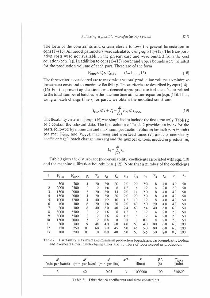
The flexibility criterion in eqn. (16) was simplified to include the first term only. Tables 2 to 5 contain the relevant data. The first column of Table 2 provides an index for the parts, followed by minimum and maximum production volumes for each part in units per year (V;MIN and V;MAx), machining and overhead times (Tii and tii), complexity coefficients (g;), batch change times (r;) and the number of tools needed in production,

4

L;= L lij. j=l

Table 3 gives the disturbance (non-availability) coefficients associated with eqn. (10) and the machine utilization bounds (eqn. (12)). Note that a number of the coefficients

ViMIN V;MAX gi 7;1 t;1 7;2 ti2 7;3 t;3 7;4 t;4 r; L;

1 500 700 4 20 2·0 20 2·0 20 2·0 8 4·0 4·0 50 2 2000 2500 2 12 1·6 6 1·2 6 1·2 4 2·0 2·0 50 3 1500 2000 3 20 2·0 14 2·0 14 2·0 8 4·0 4·0 50 4 1500 2000 4 20 2·0 20 2·0 20 2·0 8 4·0 4·0 50 5 1000 1200 4 40 1·2 10 1·2 10 1·2 8 4·0 4·0 50 6 100 300 6 20 1·6 20 2·0 40 2·0 20 4·8 4·8 50 7 200 300 8 40 2·0 40 2-4 60 2-4 40 6-0 6-0 50 8 3000 3500 2 12 1·6 6 1·2 6 1·2 4 2·0 2·0 50 9 3000 3500 2 12 1·6 6 1·2 6 1·2 4 2·0 2·0 50

10 1500 2000 3 12 0·8 8 0·8 8 0·8 8 2·0 2·0 50 11 200 300 9 48 4·0 60 4·0 60 4·0 80 6-0 6-0 100 12 150 250 10 60 5·0 45 5·0 45 5·0 80 6-0 6-0 100 13 100 200 10 0 O·O 40 5·0 60 5·5 50 8·0 8·0 100

Table2. Part family, maximum and minimum production boundaries, part complexity, tooling and overhead times, batch change times and numbers of tools needed in production.

db dg d' dPL s PL J;'MAX (min per batch) (min per facet) (min per line) (lines) (h) (min)

3 40 0·05 3 1000000 100 316800

Table 3. Disturbance coefficients and time constraints.


S9 S Sv Se h P 9 Pb Pv

($ per ($ per ($ per ($ min ($ per ($ per ($ per ($ per facet) batch) batch) mm - l) tool) facet) batch size) batch)

M qg q ($ min ($ per ($ per mm - 1

) facet) tool)

CpL

($ hr - 1)

fg

500 10 20 2 300 10 3 200 100 500 10 100 10

Table 4. Cost and flexibility coefficients.

e1 ei eJ e4

3000 3000 3000 6000

Table 5. Efficiency coefficients (mm min - 1 ).

Pareto Race

Goal 1 (max ) : prod 14750.0

Goal 2 (min ) : cost <== 2.89E+06

Goal 3 (max ) : flex <== 4 .35E+05

Bar:Accelerator F1 :Gears (8) F3:Fix nun: Turn F5:Brakes F2:Gears (F) F4:Relax F10:Exit * Goal # 1 is iq:>roved *

Figure 2. Initial solution.

in Table 3 have been aggregated, so that we do not have different values for each machine and each part, and the appropriate subscripts have been omitted. For instance,

13 4

db= I I dtj" i=lj=l

The right-most column of Table 3 gives the maximum annual production time for each machine (316 800 min). No minimum production times were specified. For simplicity, in our illustration disturbance time factors were only included in eqn. (19) at the systemwide level, and not for each machine separately.

The cost coefficients are given in Table 4. As in Table 3, some of the coefficients are aggregate measures. In our application the efficiency of each machine was measured by average tooling speed rather than calculated by using eqn. (3), and is given in Table 5.

Next we demonstrate the interactive process using the VIG package (Korhonen 1987). The model is input using spreadsheets, after which the initial efficient solution was displayed in the visual mode as in Fig. 2. In this solution, a total of 14 750 units are produced annually, and an investment of US$2 890 000 is required, while the flexibility


measure is 435 000. The figures displayed are rounded In order to evaluate these figures relative to the range of possible outcomes, the utopia and nadir values (shown in Table 6) were calculated for each criterion. The utopia value for a criterion is the best possible outcome for this criterion, regardless of the other criteria. Since the different criteria are conflicting, the utopia values for all criteria combined cannot usually be attained. The nadir value for a criterion provides a bound for its worst possible efficient outcome. Thus, the decision-maker cannot hope for a solution better than the utopia point, and will not be presented with solutions dominated by the nadir point.

Given the initial solution, the decision-maker can freely choose which goal(s) or criteria he wants to improve. Of course this means that he must sacrifice the values of some other criteria at the same time. Suppose the decision-maker is willing to accept higher investment costs in exchange for higher flexibility and a larger production volume. After indicating th~ appropriate goal directions by manipulating the arrows on the screen (see Fig. 2), the decision-maker follows the reference direction generated by the computer program. In our case, the flexibility and production criteria are emphasized, and the program projects the reference direction on the efficient frontier. We continue moving in this direction until we hit the boundaries of the efficient set. If it is still possible to improve the criterion values, the program generates a new reference direction and we can continue to improve the production and flexibility criteria. Throughout this process, the changing criterion values are visually displayed on the screen as expanding or shrinking bar graphs.

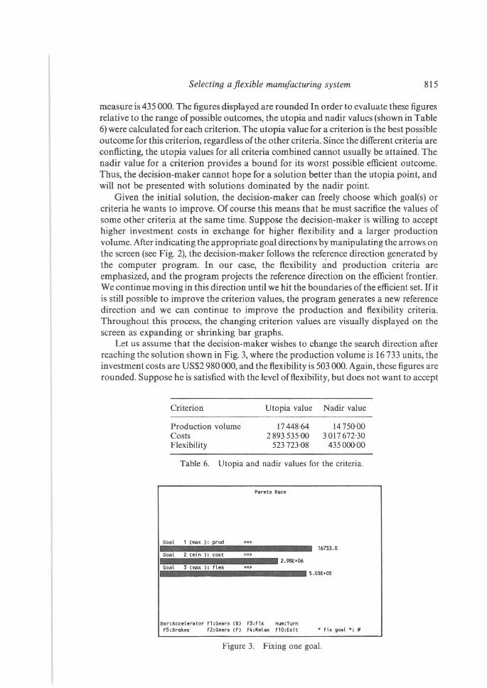
Let us assume that the decision-maker wishes to change the search direction after reaching the solution shown in Fig. 3, where the production volume is 16 733 units, the investment costs are US$2 980 000, and the flexibility is 503 000. Again, these figures are rounded. Suppose he is satisfied with the level offlexibility, but does not want to accept

Criterion

Production volume Costs Flexibility

Utopia value

17 448·64 2893 535·00

523 723·08

Nadir value

14 750·00 3017672-30

435000·00

Table 6. Utopia and nadir values for the criteria.

Pareto Race

Goal 1 (max >: prod 16733 . 0

Goal 2 (min ): cost --· 2 .98E+06

1 Goal 3 (max ): flex 5.03E+05

Bar:Accelerator F1 :Gears (8) F3 :Fix nun:Turn FS:Brakes F2:Gears (f) F4:Relax F10:Exit * Fix goal *: #

Figure 3. Fixing one goal.


values worse than the current level of 503 000. At the same time, he is willing to exchange some production volume in order to decrease the investment costs. Thus, the flexibility goal is fixed at its current level (as indicated by the star at the left of this goal in Fig. 4), and the emphasis on improving the cost criterion is indicated by changing the direction of the arrows for the cost goal on the screen.

The resulting reference direction, where both the cost goal and the production goal are decreasing, is shown in Fig. 4, so that production volume is sacrificed in exchange for lower investment costs. The decision-maker can continue to play with VIG as long as he wishes, and stop as soon as he has reached a solution with which he is satisfied. In our illustration we stopped after reaching the solution given in Fig. 5, where production volume, costs and flexibility are 16 498·90 units, US$2 970 000 and 503 000 (rounded), respectively. Note that the flexibility value in the final solution is identical to that in Fig. 4, because this goal was fixed.

Because the actions on part of the decision-maker are similar to driving a car (VIG has gears, breaks and an accelerator), the search for the 'most preferred' solution is also called a 'Pareto race' (Korhonen and Wallenius 1988). If the decision-maker so desires, he can inspect the values of the decision variables, in our case the batch sizes and

Pareto Race

Goal 1 (max ): prod 16733.0

Goal 2 (min ): cost 2.98E+06

l•Goal 3 (max ) : flex •=> 5.03E•05

Bar:Accel erator F1 :Gear& (B) Fl : Fix nun:Turn F5:Brak.es F2:Gears (F) F4 :Relax F10 :Exit * Goal II 2 ;s ;rrproved *

Figure 4. Changing the search direction.

Pareto Race

Goal 1 (max ): prod <•= . 16498. 9 Goal 2 (min >: cost <==

2.97E•06 *Goal 3 (max ) : flex =:>

5.03E+05

Bar:Accelerator F1 :Gears (8) F3 : Fix nun: Turn F5:Br akes F2:Gears (f) F4 : Relax F10:Ex f t

Figure 5. The final solution.


Name Current value

Criteria Production 16498·90 Cost 2973983·73 Flexibility 502558·96

Decision variables V1 140·00 V2 500·00 V3 400·00 V4 331·36 V5 200·00 v6 60·00 V7 60·00 Vg 600·00 V9 600·00

V10 300·00 V11 58·41 V12 30·00 V13 20·00

Machine utilization times T1 316800·00 T2 218943·25 T3 232993·25 T4 195345·40

Table 7. Values of criteria, decision variables and machine utilization times for the final solution.

number of batches produced, at any point during the solution process. The values of the criteria and decision variables for the final solution are given in Table 7. In the final solution, several of the parts (1, 2, 3, 6 and 7) are produced at their maximum level (V;MAx = b;v; = 5v;), while the production of other parts (4, 5 and 8-13) is considerably below their upper limit. Machine 1 is fully utilized (T1 =Ti max= 316 800 min), while machine 4 is only used for two-thirds of the maximum available time. These values illustrate that the solution in Fig. 6 is a compromise solution where both the production, flexibility and cost considerations are simultaneously taken into account.

5. Extensions As mentioned above, our model can be extended in a number of different ways. For

example, Ranta and Alabian (1988) and Ranta (1989) have suggested several viable additional criteria, including relative performance indicators such as the average machine time per part (TM), the average throughput time (Tu), i.e. the average time to produce a part, and unit time cost (K), i.e. the total discounted cost per period divided by the total production time per period. These criteria can be represented by

minimize J'r.1 = T / t1

b;v; (20)

minimize Tu=(T+it1

r;v;+7;i)/ t1

b;v; (21)

minimize K = ( C + L)/(T) (22)


where ri is the batch change time for part i and Lis the discounted labour, maintenance and improvement cost of the system per period.

Another issue is that, even though linear relationships are often reasonably good approximations of the true model, in some cases a non-linear formulation is preferred. In the general model described above, the non-linearities relate to the batch size and number of batches of each part. Other non-linearities which may significantly improve the model could include non-linear cost relationships and non-linear functions describing flexibility.

As mentioned above, the example given here was simplified to the linear case for ease of presentation. Since the VIG package is restricted to linear models, other software should be used if it is necessary to introduce non-linearities. One good candidate is the menu-driven and computationally powerful package IAC-DIDAS-N (Kreglewski et al. 1988). This package was designed to solve non-linear multicriteria problems, and runs on IBM-PC/XT and compatible machines. Currently the authors are experimenting with various non-linear refinements and extensions of the FMS design problem using the IAC-DIDAS-N package (Kuula and Stam 1989). Further results of these experiments, and a comparison of the results with those obtained using linear models will be reported in a future paper.

6. Conclusions In this paper a user-friendly visual interactive decision support system is introduced

which aids management in the strategic investment decision problem of which FMS configuration to acquire. The system can be used both in the initial prescreening of alternative candidate FMS designs and in the more detailed performance analysis of a select group of the most attractive candidate designs. As such, the methodology can play an important role in the predesign phase of building an FMS.

Our methodology contributes to the current literature in that it facilitates the difficult and complicated process of evaluating various types of trade-offs between multiple, potentially conflicting criteria. Both quantitative and qualitative criteria are explicitly considered in the decision process. A simple example based on a case study with real data was used to illustrate the concepts. The particular software packages used (Expert Choice and VIG) are commercially available and have been proven to be very appealing to users in numerous real-life applications. Future research should focus on non-linear refinements of the current model. In addition, the scope of the model should be extended to include more detailed information about various cost components and more accurate measures of flexibility and part complexity.

Acknowledgments This research was conducted in part while the authors were at the International

Institute for Applied Systems Analysis in Laxenburg, Austria. The authors gratefully acknowledge the support received from this organization.

References ARBEL, A., and SEIDMANN, A., 1984, Performance evaluation of flexible manufacturing systems.

IEEE Transactions on Systems, Man, and Cybernetics, 14, 606-617. BuZACOTI, J. A., and YAO, D. D., 1986, Flexible manufacturing systems: a review of analytical

models. Management Science, 32, 890-905. CHOOBINEH, F., 1986, Justification of flexible manufacturing systems. Proceedings of the 1986

International Computers in Engineering Conference and Exhibition, pp. 269-279.


DYER, R. F., FORMAN, E. A., FORMAN, E. H., and JOUFLAS, J., 1988, Marketing Decisions using Expert Choice, (McLean, VA: Decision Support Software, Inc).

FORMAN, E. H., and SAATY, T. L., 1987, Expert Choice: User's Manual (McLean, VA: Decision Support Software, Inc.).

GERSHWIN, S. B., HILDEBRANT, R. R., SURI, R., and MITTER, S. K., 1984, A control theorist's perspective on recent trends in manufacturing systems. Proceedings of the 23rd IEEE Conference on Decision and Control, Nevada, Las Vegas.

JAIKUMAR, R., 1986, Postindustrial manufacturing, Harvard Business Review, 6, 69- 79. KORHONEN, P., 1987, VIG- a visual interactive support system for multiple criteria decision

making. Belgian Journal of Operations Research, Statistics and Computer Science, 27, 3-15. KORHONEN, P ., and LAAKSO, J ., 1986, A visual interactive method for solving the multiple criteria

problem. European Journal of Operational Research, 24, 277- 287. KORHONEN, P ., and SOISMAA, M ., 1988, A multiple criteria model for pricing alcoholic beverages.

European Journal of Operational Research, 37, 165-175. KORHONEN, P ., and WALLENIUS, J., 1988, A Pareto race. Naval Research Logistics, 35, 615- 623. KREGLEWSKI, T., PACZYNSKI, J., GRANAT, J., and WIERZBICKI, A. P ., 1988, IAC-DIDAS-N: a

dynamic interactive decision analysis and support system for multicriteria analysis of nonlinear models with nonlinear model generator supporting model analysis. Working Paper No. WP-88-112, International Institute for Applied Systems Analysis, Laxenburg, Austria.

KUIVANEN, R., LEPISTO, J ., and TINSANEN, R., 1988, Disturbances in flexible manufacturing. 3rd IF AC/IFIP/IEA/IFORS Conference on Man-Machine Systems, 14-16 June, 1988, Oulu, Finland.

KuuLA, M., and STAM, A., 1989, A nonlinear multicriteria model for strategic FMS selection decisions. Working Paper No. WP-89-62, International Institute for Applied Systems Analysis, Laxenburg, Austria.

LAKSO, T., 1988, The influence of FMS-technology on the efficiency of NC-controlled machine tools. Publication No. 50, Tampere University of Technology, Tampere, Finland.

LEWANDOWSKI, A. , and WIERZBICKI, A. P., 1988, Theory, software and testing examples in decision support systems. Working Paper No. WP-88-071, International Institute for Applied Systems Analysis, Laxenburg, Austria.

LOFTI, V., 1991 , AIM-aspiration-level interactive method for multiple criteria decision making, Version 3.0, User's Guide. The University of Michigan-Flint, Flint, Michigan.

MAJCHRAZAK, J., 1988, DISCRET: an interactive decision support system for discrete alternatives multicriteria problems. Working Paper No. WP-88-113, International Institute for Applied Systems Analysis, Laxenburg, Austria.

M EREDITH, J. R., 1987 a, Implementing the automated factory. Journal of Manufacturing Systems, 6, 1- 13.

MEREDITH, J. R., 1987 b, Managing factory automation projects. Journal of Manufacturing Systems, 6, 75- 91.

NoRROS, L., TOIKKA, K., and HYOTYLAINEN, R., 1988, FMS design from the point of view of implementation: results of a case study. 3rd IFAC/IFIP/IEA/IFORS Conference on Man- Machine Systems, 14-16 June, 1988, Oulu, Finland.

RANTA, J., 1989, FMS investment as a multiobjective decision-making problem. Unpublished manuscript, International Institute for Applied Systems Analysis, Laxenburg, Austria.

RANTA, J ., and ALABIAN, A., 1988, Interactive analysis of FMS productivity and flexibility. Working Paper No. WP-88-098, International Institute for Applied Systems Analysis, Laxenburg, Austria.

RANTA, J., KOSKINEN, K., and OLLUS, M., 1988, Flexible production automation and computer integrated manufacturing: recent trends in Finland. Computers and Industry, 4, 55- 76.

SAATY, T . L., 1987, Decision Making for Leaders- The Analytic Hierarchy Process for Decisions in a Complex World (Pittsburgh, PA: University of Pittsburgh Press).

SAATY, T. L., 1980, The Analytic Hierarchy Process (New York: McGraw-Hill). STAM, A., JOACHIMSTHALER, E. A., and GARDINER, L. R., 1987, An interactive decision support for

sales resource allocation with multiple objectives: an exploratory study. Working Paper No. 87- 243. College of Business Administration, University of Georgia.

STEUER, R. E., 1986, Multiple Criteria Optimization: Theory, Computation and Application (New York: Wiley).

820 Selecting a flexible manufacturing system

WABALICKIS, R. N., 1988, Justification of FMS with the analytic hierarchy process. Journal of Manufacturing Systems, 7, 175- 182.

WHITNEY, C., 1985, Control principles in flexible manufacturing. Journal of Manufacturing Systems, 4, 157- 167.

WIERZBICKI, A. P., 1979, A methodological guide to multiobjective decision making. Working Paper No. WP-79-122, International Institute for Applied Systems Analysis, Laxenburg, Austria.

WIERZBICKI, A. P ., 1982, A mathematical basis for satisficing decision making. Mathematical Modelling, 3, 391-405.

Documents

SELECTING A FLEXIBLE MANUFACTURING …pure.iiasa.ac.at/3495/1/RR-91-20.pdfSELECTING A FLEXIBLE MANUFACTURING SYSTEM USING MULTIPLE CRITERIA ... such relevant performance criteria as