SELECTED CHAPTERS OF GEOMETY, ANALYSIS AND NUMBER THEORY · PDF fileSELECTED CHAPTERS OF GEOMETY, ANALYSIS AND NUMBER THEORY by ... Bernoulli numbers, perfect numbers and generalizations,

SELECTED CHAPTERSOF GEOMETY, ANALYSISAND NUMBER THEORY

by

Jozsef Sandor

2005

”... There is no study in the world which brings into more harmoniousaction all the faculties of the mind than mathematics... or like this, seems toraise them, by successive steps of initiation, to higher and higher states ofconscious intellectual being...”

(James J. Sylvester)

1

2

Preface

The aim of this book is to present short notes or articles, as well as stud-ies on some topics of Geometry, Analysis, and Number Theory. The materialis divided into ten chapters: Geometry and geometric inequalities; Sequencesand series of real numbers; Special numbers and sequences of integers; Al-gebraic and analytic inequalities; Euler gamma function; Means and meanvalue theorems; Functional equations and inequalities; Diophantine equations;Arithmetic functions; and Miscellaneous themes. Chapter 1 deals essentiallywith classical geometric properties of triangles, polygons and tetrahedrons,as well as trigonometric functions. There are included some recent advancesin triangle and tetrahedron inequalities, due to the author. Chapter 2 stud-ies certain sequences and series of real numbers. Paragraph 2 includes somestrange sequences, having interesting definitions and properties. Other themesintroduce the Wallis product, Olivier’s criterion, Dirichlet’s beta function, orBereznai’s theorem on the convergence or divergence of infinite series. The spe-cial numbers and sequences of integers of Chapter 3 require special methods ofNumber theory. Here some properties of the sequence of primes, of compositenumbers, Bernoulli numbers, perfect numbers and generalizations, or abun-dant and deficient numbers, are studied. Chapter 4 discusses various algebraicand analytic inequalities, as the Cauchy-Bunjakovski, Chrystal’s, Hadamard’s,Jensen’s, Chebyshev’s, Fink’s, Ky Fan’s, Alzer’s, etc. inequalities, with manyconnections and applications to other fields. Chapter 5 contains 16 notes onthe famous Euler gamma function. Many basic as well as new properties (dueto the author), including monotonicity or convexity are studied. Papers 11-13have been used by many authors in various fields of study, including Discretemathematics, Number theory, Analysis, Linear Algebra, etc. Chapter 6 studiescertain new mean value theorems, as well as mean values, with applications. Aspecial attention is given to applications of Cauchy’s mean value theorem, aswell as certain special means, including the so called logarithmic and identricmeans, or the Seiffert means. The first theme of Chapter 7 on the Bohr-Mollerup theorem could have been considered also in Chapter 5 on Euler’sgamma function. Here the emphasis is however on functional equations, andalong with the classical gamma function, the q-gamma function of Jackson isalso involved. The other themes of this chapter rely on functional equations of

3

more unknowns as Cauchy’s, Haruki’s and Cioranescu’s, Rassias’ or Bartha’sfunctional equations. Some functional inequalities are studied, too. Chapter8 contains certain Diophantine equations of a new type. The Pell type equa-tions, as well as cubic equations of many unknowns are included. There arealso other interesting equations involving factorials (based on a problem bySmarandache), or arithmetic functions ϕ, σ, ψ. Paragraph 10 introduces a newconcept of Geometry and Number theory: harmonic triangles. A large chapterinvolving various arithmetic functions is Chapter 9. Here many properties ofthe classical functions as Euler’s totient, the sum and numberof divisors,Jordan’s totient, the Smarandache function, etc. are introduced. There areconsidered also many new arithmetic functions, as the Euler minimum andmaximum functions, the Smarandache minimum and maximum functions, thestar function of an arithmetic function, etc. Finally, Chapter 10 deals withvarious miscellaneous themes, as Fermat’s ”little” theorem and its generaliza-tions, Euler pretty numbers, or certain inequalities of Klamkin, Ky Fan, orLehman’s, with applications. Article 2 introduces the geometric numbers, notpublished elsewhere.

The majority of the included material is original, based on papers by theauthor. Some of them have been published in some little known journals ofRomania and Hungary, or in known journals from Bulgaria, Yugoslavia, Ger-many, Suisse, India, Australia, and USA. The book is concluded with an authorindex, focused on articles (and not pages), where the same author may appearmore times.

Finally, I wish to express my gratitude to a number of persons and orga-nizations from whom I received valuable advice or support in the preparationof this book. These are the Mathematics and Informatics Departments of theBabes-Bolyai University of Cluj (Romania), the Domus Hungarica Foundationof Budapest, the Sapientia Foundation and the Bolyai Society of Cluj; and alsoProfessors H. Alzer, J. Aczel, T. Andreescu, K.T. Atanassov, M. Bencze, M.Balazs, W.W. Breckner, G.L. Cohen, P. Erdos, L. Filep, R.K. Guy, I. Katai, J.Kolumban, M.S. Klamkin, H.J. Kanold, A. Lupas, R. Laatsch, Gy. Maurer, A.Makowski, E. Neuman, C. Pomerance, G. Robin, I.Z. Ruzsa, I. Rasa, Th.M.Rassias, H.J.J. te Riele, K.B. Stolarsky, F. Smarandache, R.M. Sorli, M.V.Subbarao, H.N. Shapiro, A. Schinzel, H.J. Seiffert, L. Toth, Gh. Toader, J.Wendel, I. Virag, M. Vuorinen, F.A. Valentine, A. Vernescu.

The camera-ready manuscript for the present book was prepared by Mrs.Georgeta Bonda (Cluj) to whom the author expresses his gratitude.

16th August, 2005 The author

4

Contents

Preface 3

1 Geometry and geometric inequalities 111 A property of polygons . . . . . . . . . . . . . . . . . . . . . . . 122 On a theorem of Cotes in elementary geometry . . . . . . . . . 133 On some new geometric inequalities . . . . . . . . . . . . . . . 154 Some inequalities for the elements of a triangle . . . . . . . . . 19

5 Recent advances in triangle inequalities . . . . . . . . . . . . . 226 The cotangent inequality of a triangle . . . . . . . . . . . . . . 27

7 On∏

sinA

2≤∏

cosA−B

2. . . . . . . . . . . . . . . . . . . 31

8 The sum of medians, and angle bysectors . . . . . . . . . . . . 329 On a generalization of the Erdos-Mordell inequality . . . . . . . 3410 On certain inequalities in a tetrahedron . . . . . . . . . . . . . 3511 Certain trigonometric inequalities deduced by convexity

methods . . . . . . . . . . . . . . . . . . . . . . . . . . . . . . . 4012 On some trigonometric inequalities of Bencze . . . . . . . . . . 49

13 Onsinx

x. . . . . . . . . . . . . . . . . . . . . . . . . . . . . . . 52

14 On de Cusa’s trigonometric inequality . . . . . . . . . . . . . . 53

15 A property of sin1

x. . . . . . . . . . . . . . . . . . . . . . . . . 54

16 (sinx)cos x + (cos x)sin x made integer . . . . . . . . . . . . . . . 55

2 Sequences and series of real numbers 571 On certain limits related to the number e . . . . . . . . . . . . 582 On some strange sequences . . . . . . . . . . . . . . . . . . . . 643 Determination of certain sequences . . . . . . . . . . . . . . . . 90

4 A sequence connected with the Wallis product . . . . . . . . . 925 A generalized ratio test for series of positive terms . . . . . . . 946 A generalization of Bereznai’s theorem on infinite series . . . . 95

5

7 The iteration of sin and cos and two infinite series . . . . . . . 98

8 On Olivier’s criterion . . . . . . . . . . . . . . . . . . . . . . . . 99

9 On Dirichlet’s beta function . . . . . . . . . . . . . . . . . . . . 101

10 On sequences related to the sum of powers of positiveintegers . . . . . . . . . . . . . . . . . . . . . . . . . . . . . . . 102

3 Special numbers and sequences of integers 105

1 On pn/ ln n . . . . . . . . . . . . . . . . . . . . . . . . . . . . . 106

2 On the integer part of n√pk . . . . . . . . . . . . . . . . . . . . 107

3 [ex] and [ey] as consecutive primes . . . . . . . . . . . . . . . . 108

4 On a sequence connected with the number of primes . . . . . . 108

5 The smallest number of ones . . . . . . . . . . . . . . . . . . . 109

6 On the sequence of composite numbers . . . . . . . . . . . . . . 110

7 A note on Bernoulli numbers . . . . . . . . . . . . . . . . . . . 112

8 The number of factorizations of n . . . . . . . . . . . . . . . . . 113

9 On perfect and m-perfect numbers . . . . . . . . . . . . . . . . 114

10 On Ruzsa’s lovely pairs . . . . . . . . . . . . . . . . . . . . . . 116

11 Completely d-perfect numbers . . . . . . . . . . . . . . . . . . . 118

12 On completely f -perfect numbers . . . . . . . . . . . . . . . . . 121

13 On (f, g)-perfect numbers . . . . . . . . . . . . . . . . . . . . . 126

14 On abundant and deficient numbers . . . . . . . . . . . . . . . 130

15 On abundant and nobly-abundant, or deficient numbers . . . . 132

16 The numbers n for which σ(n), d(n), ϕ(n) are abundant ordeficient . . . . . . . . . . . . . . . . . . . . . . . . . . . . . . . 134

17 On S-abundant and deficient numbers . . . . . . . . . . . . . . 137

18 The square deficiency of a number . . . . . . . . . . . . . . . . 139

19 Exponentially harmonic numbers . . . . . . . . . . . . . . . . . 141

4 Algebraic and analytic inequalities 147

1 A monotonicity property of a product of sums of powers . . . . 148

2 An application of the Cauchy-Bunjakovski inequality . . . . . . 148

3 The Chrystal inequality and its applications to convexity . . . 150

4 On certain inequalities for square roots and n-th roots . . . . . 152

5 On evaluation ofk∑

i=1

n√i . . . . . . . . . . . . . . . . . . . . . . 155

6 The product of consecutive odd integers . . . . . . . . . . . . . 157

7 On Hadamard’s inequality . . . . . . . . . . . . . . . . . . . . . 159

8 On certain inequalities for the number e . . . . . . . . . . . . . 163

9 The Jensen integral inequality . . . . . . . . . . . . . . . . . . . 165

6

10 Generalizations of certain integral inequalities . . . . . . . . . . 169

11 The Chebyshev integral inequality . . . . . . . . . . . . . . . . 175

12 On Fink’s inequality . . . . . . . . . . . . . . . . . . . . . . . . 17813 An extension of Ky Fan’s inequalities . . . . . . . . . . . . . . . 179

14 A converse of Ky Fan’s inequality . . . . . . . . . . . . . . . . . 182

15 A refinement of Gn +G′n ≤ 1 . . . . . . . . . . . . . . . . . . . 183

16 On Alzer’s inequality . . . . . . . . . . . . . . . . . . . . . . . . 184

5 Euler gamma function 187

1 A limit involving the Gamma function and the Lalescusequence . . . . . . . . . . . . . . . . . . . . . . . . . . . . . . . 188

2 On a sequence containing the Gamma function . . . . . . . . . 1883 The product of consecutive factorials . . . . . . . . . . . . . . . 189

4 On Γ(kn) . . . . . . . . . . . . . . . . . . . . . . . . . . . . . . 190

5 On a limit for the quotients of Gamma functions . . . . . . . . 192

6 A limit for the Euler-Beta function . . . . . . . . . . . . . . . . 195

7 On convex functions involving Euler’s Gamma function . . . . 1978 A convexity result on (f(x))1/x . . . . . . . . . . . . . . . . . . 198

9 On a subadditive property of the Gamma function . . . . . . . 200

10 A convexity property of the Gamma function . . . . . . . . . . 201

11 Monotonicity and convexity (concavity) of some functionsrelated to the Gamma function . . . . . . . . . . . . . . . . . . 202

12 On the Gamma function II . . . . . . . . . . . . . . . . . . . . 210

13 On the Gamma function III . . . . . . . . . . . . . . . . . . . . 214

14 On certain inequalities for the ratios of Gamma functions . . . 221

15 A note on certain inequalities for the Gamma function . . . . . 224

16 Gamma function inequalities and traffic flow . . . . . . . . . . 226

6 Means and mean value theorems 229

1 Monotonicity and convexity properties of means . . . . . . . . 230

2 Logarithmic convexity of the means It and Lt . . . . . . . . . . 2373 On certain subhomogeneous means . . . . . . . . . . . . . . . . 240

4 On a method of Steiner . . . . . . . . . . . . . . . . . . . . . . 248

5 On Karamata’s and Leach-Sholander’s theorems on means . . . 250

6 Certain logarithmic means . . . . . . . . . . . . . . . . . . . . . 251

7 The arithmetic-geometric mean of Gauss . . . . . . . . . . . . . 2568 On two means by Seiffert . . . . . . . . . . . . . . . . . . . . . 265

9 Some new inequalities for means and convex functions . . . . . 268

10 On an inequality of Sierpinski on the arithmetic, geometric andharmonic means . . . . . . . . . . . . . . . . . . . . . . . . . . 272

7

11 An application of Rolle’s theorem . . . . . . . . . . . . . . . . . 274

12 An application of Lagrange’s mean value theorem for thecomputation of a limit . . . . . . . . . . . . . . . . . . . . . . . 278

13 An inequality of Alzer, as an application of Cauchy’s mean valuetheorem . . . . . . . . . . . . . . . . . . . . . . . . . . . . . . . 278

14 A new mean value theorem . . . . . . . . . . . . . . . . . . . . 279

15 Some mean value theorems and consequences . . . . . . . . . . 283

16 The second mean value theorem of integral calculus . . . . . . 290

7 Functional equations and inequalities 297

1 The Bohr-Mollerup theorem . . . . . . . . . . . . . . . . . . . . 298

2 On certain functional equations containing more unknownfunctions . . . . . . . . . . . . . . . . . . . . . . . . . . . . . . 303

3 Locally integrable solutions of Cauchy’s functionalequation . . . . . . . . . . . . . . . . . . . . . . . . . . . . . . . 306

4 Generalizations of Haruki’s and Cioranescu’s functionalequations . . . . . . . . . . . . . . . . . . . . . . . . . . . . . . 307

5 The functional equation f

(n∑

k=1

xk

)

=

n∑

k=1

(f(xk))k . . . . . . . 311

6 Two functional equations . . . . . . . . . . . . . . . . . . . . . 313

7 A functional equation satisfied by the sin and identityfunctions . . . . . . . . . . . . . . . . . . . . . . . . . . . . . . 315

8 On certain functional equations by Rassias . . . . . . . . . . . 317

9 Bartha’s functional equation . . . . . . . . . . . . . . . . . . . . 319

10 An application of Chebyshev’s inequality . . . . . . . . . . . . . 320

11 On a functional inequality . . . . . . . . . . . . . . . . . . . . . 321

12 An unsolved functional equation . . . . . . . . . . . . . . . . . 321

8 Diophantine equations 323

1 Variations on a problem with factorials . . . . . . . . . . . . . . 324

2 On the Diophantine equationx1x2 + x2x3 + · · · + xnx1 = n+ x1 + · · · + xn . . . . . . . . . . 327

3 On the equation n+ (n+ 1) + · · · + (n+ k) = n(n+ k) . . . . 329

4 On a problem of Subramanian, and Pell equations . . . . . . . 330

5 On the Diophantine equation x3 + y3 + z3 = a . . . . . . . . . 332

6 On the Diophantine equation x3 + y3 + z3 = a, II . . . . . . . . 333

7 n dimensional cuboids with integer sides and diagonals . . . . . 336

8 The equation x2 + y2 = z2 . . . . . . . . . . . . . . . . . 337

9 On the Diophantine equation1

x1+

1

x2+ · · · + 1

xn=a

b. . . . . 338

8

10 Harmonic triangles . . . . . . . . . . . . . . . . . . . . . . . . . 341

11 A Diophantine equation involving Euler’s totient . . . . . . . . 343

12 On f(n) + f(n+ 1) + · · · + f(n+ k) = f(n)f(n+ k)for f ∈ ϕ,ψ, σ . . . . . . . . . . . . . . . . . . . . . . . . . . 346

13 On certain equations for the Euler, Dedekind, andSmarandache functions . . . . . . . . . . . . . . . . . . . . . . . 350

14 Some equations involving the arithmetical functions ϕ, σ, ψ . . 350

15 Equations with composite functions . . . . . . . . . . . . . . . 351

16 On d(n) + σ(n) = 2n . . . . . . . . . . . . . . . . . . . . . . . . 353

9 Arithmetic functions 357

1 The non-Lipschitz property of certain arithmetic functions . . . 3582 On certain open problems considered by Murthy . . . . . . . . 359

3 On an inequality of Moree on d(n) . . . . . . . . . . . . . . . . 361

4 On duals of the Smarandache simple function . . . . . . . . . . 363

5 A modification of the Smarandache function . . . . . . . . . . . 366

6 The star function of an arithmetic function . . . . . . . . . . . 369

7 On Jordan’s arithmetical function . . . . . . . . . . . . . . . . 372

8 Generalization of a theorem of Lucas on Euler’s totient . . . . . 3779 Some arithmetic inequalities connected with the divisors of

an integer . . . . . . . . . . . . . . . . . . . . . . . . . . . . . . 379

10 A new arithmetic function . . . . . . . . . . . . . . . . . . . . . 382

11 A generalization of Ruzsa’s theorem . . . . . . . . . . . . . . . 388

12 On the monotonicity of the sequence (σk/σ∗k) . . . . . . . . . . 389

13 A note on exponential divisors and related arithmeticfunctions . . . . . . . . . . . . . . . . . . . . . . . . . . . . . . 393

14 The Euler minimum and maximum functions . . . . . . . . . . 39815 The Smarandache minimum and maximum functions . . . . . . 403

16 The pseudo-Smarandache minimum and maximumfunctions . . . . . . . . . . . . . . . . . . . . . . . . . . . . . . 408

10 Miscellaneous themes 413

1 On a divisibility problem . . . . . . . . . . . . . . . . . . . . . 414

2 A generalization of Fermat’s little theorem . . . . . . . . . . . . 4143 On an inequality of Klamkin . . . . . . . . . . . . . . . . . . . 416

4 Euler-pretty numbers . . . . . . . . . . . . . . . . . . . . . . . . 422

5 Abundant numbers involving the smallest and largest primefactors . . . . . . . . . . . . . . . . . . . . . . . . . . . . . . . . 423

6 An inequality with shx and chx . . . . . . . . . . . . . . . . . 424

7 On geometric numbers . . . . . . . . . . . . . . . . . . . . . . . 425

9

8 The sum-of-divisors minimum and maximum functions . . . . . 4319 On certain new means and their Ky Fan type inequalities . . . 43810 On Lehman’s inequality and electrical networks . . . . . . . . . 446

Author Index 455

10

Chapter 1

Geometry and geometricinequalities

”... Nothing is more important than to see the sources of invention whichare, in my opinion more interesting than the inventions themselves.”

(Gottfried Leibnitz)

”... As long as algebra and geometry have been separated, their progresshave been slow and their uses limited; but when these two sciences have beenunited, they have lent each mutual forces, and have marched together towardsperfection.”

(Joseph-L. Lagrange)

11

1 A property of polygons

Let A1A2 . . . An be a convex polygon in the plane and P an arbitrary point.We will study the equality

n∑

k=1

(−1)kPA2k = 0. (1)

First, we show that n must be even. Indeed, let the coordinates ofAk(ak, bk), while P (x, y). Then (1) is written equivalently as

(x− a1)2 + (y − b1)

2 + (x− a3)2 + (y − b3)

2 + · · · =

= (x− a2)2 + (y − b2)

2 + (x− a4)2 + (y − b4)

2 + . . .

If n would be odd, then this equation would be the equation of circle, andclearly if P is not on this circle, relation (1) cannot be satisfied. Let n = 2kbe even. Then the above equation gives:

−2x(a1 + a3 + · · · + a2k−1)− 2y(b1 + b3 + · · · + b2k−1) + a21 + a2

3 + · · · + a22k−1

+b21 + · · · + b22k−1 = −2x(a2 + a4 + · · · + a2k) − 2y(b2 + b4 + · · · + b2k)

+a22 + a2

4 + · · · + a22k + b22 + b24 + · · · + b22k.

This clearly implies

a1 + a3 + · · · + a2k−1 = a2 + a4 + · · · + a2k

b1 + b3 + · · · + b2k−1 = b2 + b4 + · · · + b2k

a21 + a2

3 + · · · + a22k−1 + b21 + b23 + · · · + b22k−1 =

= a22 + a2

4 + · · · + a22k + b22 + b24 + · · · + b22k

(2)

Therefore, conditions (2) are necessary and sufficient that (1) hold forarbitrary (fixed) points Ak. However, for a more transparent geometric study,we shall use the vectorial method.

Let O 6= P another point with property (1). Then, since

−−→PAi =

−−→PO +

−−→OAi, i = 1, 2k,

we get

PA2i = PO2 +OA2

i + 2−−→PO · −−→OAi,

giving:

PA21 + PA2

3 + · · · + PA22k−1 − (PA2

2 + PA24 + · · · + PA2

2k)

12

= OA21 +OA2

3 + · · · +OA22k−1 − (OA2

2 +OA24 + · · · +OA2

2k)

+2−−→PO[(

−−→OA1 +

−−→OA3 + · · · + −−−−−→

OA2k−1) − (−−→OA2 +

−−→OA4 + · · · + −−−→

OA2k)].

Since P and O satisfy (1) and P 6= O, we get:

−−→OA1 +

−−→OA3 + · · · + −−−−−→

OA2k−1 =−−→OA2 +

−−→OA4 + · · · + −−−→

OA2k. (3)

Let G1, G2 be the centroids of polygons A1A3 . . . A2k−1 and A2A4 . . . A2k, re-spectively. Since

−−→OA1 +

−−→OA3 + · · · + −−−−−→

OA2k−1 = k−−→OG1 +

−−−→G1A1 +

−−−→G1A3 + · · · + −−−−−−→

G1A2k−1

and

−−→OA2 +

−−→OA4 + · · · + −−−→

OA2k = k−−→OG2 +

−−−→G2A2 +

−−−→G2A4 + · · · + −−−−→

G2A2k

and −−−→G1A1 + · · · + −−−−−−→

G1A2k−1 =−−−→G2A2 + · · · + −−−−→

G2A2k = 0,

we get−−→OG1 =

−−→OG2, i.e.

−−−→G1G2 = 0, implying G1 ≡ G2. Therefore (3) means

that the centroids of the above polygons must coincide. For example, whenn = 4 (k = 2), we get a parallelogram, and condition OA2

1+OA23 = OA2

2+OA24

yields that this must be a rectangle. When n = 6 (k = 3), an example for which(1) is true is the regular hexagon, since then we may take O to be the centreof circumscribed circle when all conditions are satisfied.

2 On a theorem of Cotes in elementary geometry

Let (C) be a circle with centre O and radius r; let A0, A1, A2, . . . , A2m−1,A2m ≡ A0 be points on the circumference dividing it into 2m equal parts. If Kis an arbitrary point of the diameter A0Am, then R. Cotes (1682-1716) provedthe following formulae:

KA1 ·KA3 . . . KA2m−1 = rm ± xm,

KA0 ·KA2 . . . KA2m = rm ± xm,

where x = OK, and the sign depends on the parity of m and the position ofK to the point O (see also [1]).

In what follows, the following generalization will be deduced.

13

Theorem. Let (X,+, ·) be a commutative field and let (X∗, ·) be the mul-tiplicative subgroup of X. Let G = ai : i = 1, 2, . . . , n be a finite subgroup ofX∗. If 1 ∈ G is the unity element of G, then the following identity holds true:

n∏

i=1

(x+ tai) = xn + (−1)n−1tn, x, t ∈ X arbitrary.

Proof. We will apply Fermat’s theorem for finite groups: If the order ofthe finite group G is N , then gN = 1 for all g ∈ G (see [2]).

Let us consider the polynomial P (u) = un + (−1)n−1tn (u ∈ X). We’llprove that xi = −tai (i = 1, 2, . . . , n) are roots for P . Indeed, by using theproperties of field X and the above theorem of Fermat, one has:

P (xi) = (−tai)n + (−1)n−1tn = (−1)ntnan

i + (−1)n−1tn

= tn[(−1)n + (−1)n−1] = tn · 0 = 0,

where 0 is the neutral element of X. Now, Bezout’s theorem implies the statedidentity.

We now prove that Cotes’ theorem is a consequence of this result. Letthe affixes of the points Ak in the complex plane be Ak(re

kiπ/m) (where i2 =−1) and of K be a K(a); and let us consider the set G of numbers a0 =ei·0π/m, a2 = ei2π/m, . . . , a2m−2 = ei(2m−2)π/m. It is immediate that (G, ·) is afinite subgroup of the multiplicative group (C∗, ·) of nonzero complex numbers(indeed: asat ∈ G, a−1

s = as, s, t = 0, . . . ,m− 2). By the Theorem one has

n−1∏

k=0

KA2k = |am + (−1)m(−r)m|.

We have two situations: If K and A0 are on the same part with respectto O, when a > 0, a = x and r > x, so the result is rm − xm, in the secondcase K and A0 are in distinct sides of the diameter with respect to O, thena = −x, so if m is even the result is rm − xm; but rm + xm if m is odd.

Applying the theorem to the finite group of roots of unity of order 2m weget:

2m−1∏

k=0

KAk = |r2m − a2m| = r2m − x2m

(since 2m is even). Therefore

m∏

k=1

KA2k−1 =r2m − x2m

m−1∏

k=0

KA2k

=r2m − x2m

rm ± xm= rm + xm

14

in case 1), while in case 2) we get rm + xm for m even, rm − xm for m odd.

References

[1] The Pallas Great Lexicon (Hungarian), Budapest, 1983, IV, 542.

[2] Gy. Maurer, I. Virag, Introduction to structure theory (Hungarian), Ed.Dacia, Cluj, 1976.

3 On some new geometric inequalities

1. Let ABC be a triangle with standard notations, see e.g. our paper [3].Let ha, hb, hc be the altitudes; ma,mb,mc the medians; and la, lb, lc the anglebisectors of the triangle. Let T = area(ABC). In the book [2] (Result 2.12) itis proved the following implication

a ≥ b ⇒ a+ ha ≥ b+ hb. (1)

Pal Erdos raised the problem

a > b > c?⇒ a+ la > b+ lb > c+ lc,

and Bela Finta [1] infirmed this property. Of course, remains open the problemof characterization of

a ≥ b?⇒ a+ la ≥ b+ lb. (2)

In this section we shall obtain certain results of type (1) and (2). As ageneralization of (1), the following is true

a ≥ b ⇒ aα + hαa ≥ bα + hα

b (3)

for all α ∈ R. Indeed, let α > 0. Then, since aha = bhb = 2T , the inequalityto be proved becomes

aα − bα ≥ (2T )α(aα − bα)

(ab)α,

which is equivalent to ab ≥ 2T . This is valid, since 2T = ab sinC ≤ ab. Whenα < 0, put α = −β, and remark that a−β + h−β

a ≥ b−β + h−βb is equivalent to

hβa + aβ ≥ hβ

b + bβ (β > 0) which has been proved above. Thus (3) holds truefor all real numbers α.

15

2. General situations, such in (3), are very rare, and difficult to obtain.For ma or la we shall consider mainly the case α = 2. First we prove anotherelementary, but nice fact

a ≥ b ⇒ a2 +m2a ≥ b2 +m2

b . (4)

By m2a =

1

4[2(b2 + c2) − a2], etc., we have

a2 +m2a =

2b2 + 2c2 + 3a2

4and b2 +m2

b =2a2 + 2c2 + 3b2

4,

so

2b2 + 2c2 + 3a2 ≥ 2a2 + 2c2 + 3b2 ⇔ a2 ≥ b2 ⇔ a ≥ b.

On the other hand, a multiplicative analog stand as follows:If a ≥ b, then ama ≥ bmb iff (5)

a2 + b2 ≤ 2c2 (∗)

Indeed,

a2m2a ≥ b2m2

b ⇔ a2

4[2(b2 + c2) − a2] ≥ b2

4[2(a2 + c2) − b2] ⇔

2a2c2 − a4 ≥ 2b2c2 − b4 ⇔ b4 − a4 + 2c2(a2 − b2) ≥ 0 ⇔

(a2 − b2)[2c2 − (a2 + b2)] ≥ 0 ⇔ 2c2 ≥ a2 + b2.

Remark. If m(C) ≥ 90, then inequality (∗) is true. Indeed, in this case itis known the inequality a+ b ≤ c

√2 (see our monograph [2]). Thus a2 + b2 <

(a+ b)2 ≤ 2c2.3. A multiplicative analog involving la holds only when certain additional

conditions are satisfied:If a ≥ b and m(C) ≤ 60 or m(C) ≥ 90, then ala ≤ blb. (6)If a ≥ b and 60 ≤ m(C) ≤ 90, then ala ≥ blb. (7)By using the classical formulae for l2a, we can write successively

a2l2a =2a2bcp(b+ c− a)

(b+ c)2≥ 2b2acp(c+ a− b)

(a+ c)2= b2l2b

iffa(b+ c− a)

(b+ c)2≥ b(c+ a− b)

(a+ c)2.

16

Let

x =b

a+ c, y =

a

b+ c.

Then the above inequality can be written as

y − y2 ≥ x− x2 or (x− y)(x+ y − 1) ≥ 0.

But

x− y =b

a+ c− a

b+ c=

(b− a)(b+ a+ c)

(a+ c)(b+ c)≤ 0

(after certain elementary calculations) if a ≥ b. On the other hand x+ y ≤ 1can be written as

b2 + bc+ a2 + ac ≤ ab+ ac+ cb+ c2 or a2 + b2 − ab ≤ c2.

By using the law of cosines, c2 = a2 + b2 −2ab cosC, thus cosC ≤ 1

2which

is true only if m(C) ≤ 60 or m(C) ≥ 90.4. We now remark that

a ≥ b ⇒ a+ma ≥ m+mb (8)

iff

ma +mb ≥3

4(a+ b). (∗∗)

Indeed,

a+ma ≥ b+mb ⇔ 2a+√

2(b2 + c2) − a2 ≥ 2b+√

2(a2 + c2) − b2

or2(a− b) ≥

√2(a2 + c2) − b2 −

√2(b2 + c2) − a2

=[2(a2 + c2) − b2] − [2(b2 + c2) − a2]√2(a2 + c2) − b2 +

√2(b2 + c2) − a2

=3(a2 − b2)√

2(a2 + c2) − b2 +√

2(b2 + c2) − a2.

By simplifying with a− b > 0, we get ma +mb ≥ 34(a+ b).

Remarks. 1) it is easy to see that in all triangles ABC one has ma +mb ≥3c2 . Since

3c

2≥ 3

4(a + b) ⇔ a + b ≤ 2c, we get the following corollary (by

taking into account of (∗∗))If a ≥ b and a+ b ≤ 2c, then a+ma ≥ b+mb. (9)

17

2) Let G be the centroid of the triangle ABC, and let A′ = AG ∩ BC,BD‖CG, CD‖BG. Then, it is easy to see, that in BGD:

BG =2

3mb, BD = GC =

2

3mc, GD = 2 · 1

3ma =

2

3ma.

Since C ′A′ + BA′ =a+ b

2(where C ′ is the midpoint of [AB]) then ma +

mb ≥ 34(a+ b) can be written as BG+GD ≥ C ′A′ +BA′. This must be true

in the trapezium C ′GDB. Clearly, this is not generally valid, so the inequality(8) itself is valid under additional conditions.

3) Another remark is that in GDB, from BG + GD > BD we get

ma +mb > mc. Assuming that m(BGD) ≥ 90, it is well known (see [2], p.47)

that ma +mb ≤√

2mc. Since mc <a+ b

2and

√2

2<

3

4, we get the following

corollary:If m(BGD) ≥ 90, and a ≥ b, then a+ma ≤ b+mb. (10)5. We now prove that

a ≥ b ⇒ a2 + l2a ≥ b2 + l2b (11)

iff

c(a+ b+ c)(c3 + ba2 +ab2 + bc2 +ac2 +3abc) ≤ (b+a)(a+ c)2(b+ c)2. (∗ ∗ ∗)

Indeed, by using the formula

la =2

b+ c

√bcp(p− a),

one gets

l2a + l2b = (b− a)(c3 + ba2 + bc2 + ab2 + ac2 + 3abc)c(a+ b+ c)

(a + c)2(b+ c)2

≥ (b− a)(b− a)

if (∗ ∗ ∗) is valid.Remark. Thus, the problem which arises here, is the validity of condition

(∗ ∗ ∗). The analogous linear variant is the followinga ≥ b ⇒ a+ la ≥ b+ lb iff (12)

la + lb ≥ δ(a, b, c), (∗ ∗ ∗∗)

18

where

δ(a, b, c) = (c3 + 3abc+ ba2 + ab2 + bc2 + ac2)a(a+ b+ c)

(a+ c)2(b+ c)2.

We have proved above that

l2a − l2b = (b− a)δ(a, b, c),

thus

la − lb =(b− a)δ(a, b, c)

la + lb≥ b− a ⇔ δ(a, b, c) ≤ la + lb.

Problems. The study of expression δ(a, b, c). For example, since it isknown that la+lb ≤ p

√3−mc (see [2], p.49) one can ask, under what conditions

do we have

p√

3 −mc ≤ δ? (13)

One can ask, if p√

3 − δ has a constant sign, or

δ < p√

3? (14)

A similar question is the following one: if a ≥ b, under what conditionscan be written the inequality δ ≤ a + b? Of course, one can raise problemsfor relations (4), etc. by asking conditions for a ≥ b ⇒ aα +mα

a ≥ bα +mαb

(α ∈ R, for example).

References

[1] B. Finta, A solution for an elementary open question of Pal Erdos, Oc-togon Math. Mag., 4(1996), no.1, 74-79.

[2] J. Sandor, Geometric inequalities (Hungarian), Ed. Dacia, Cluj, 1988.

[3] J. Sandor, On certain inequalities for the distances of a point to thevertices and the sides of a triangle, Octogon Math. Mag., 5(1997), no.1,19-23.

4 Some inequalities for the elements of a triangle

In this section certain new inequalities for the angles (in radians) and otherelements of a triangle are given. For such inequalities we quote the monographs[2] and [3].

19

1. Let us consider the function

f(x) =x

sinx, 0 < x < π

and its first derivative

f ′(x) =1

sinx(sinx− x cos x) > 0.

Hence the function f is monotonous nondecreasing on (0, π), so that onecan write f(B) ≤ f(A) for A ≤ B, i.e.

B

b≤ A

a, (1)

because of sinB =b

2Rand sinA =

a

2R. Then, since B ≤ A if b ≤ a, (1)

implies the relation

(i)A

B≥ a

b, if a ≥ b.

2. Assume, without loss of generality, that a ≥ b ≥ c. Then in view of (i),

A

a≥ B

b≥ C

c,

and consequently

(a− b)

(A

a− B

b

)≥ 0, (b− c)

(B

b− C

c

)≥ 0, (c− a)

(C

c− A

a

)≥ 0.

Adding these inequalities, we obtain

∑(a− b)

(A

a− B

b

)≥ 0,

i.e.

2(A +B + C) ≥∑

(b+ c)A

a.

Adding A + B + C to both sides of this inequality, and by taking intoaccount of A+B +C = π, and a+ b+ c = 2s (where s is the semi-perimeterof the triangle) we get

(ii)∑ A

a≤ 3π

2s.

This may be compared with Nedelcu’s inequality (see [3], p.212)

(ii)’∑ A

a<

3π

4R.

20

Another inequality of Nedelcu says that

(ii)”∑ 1

A>

2s

πr.

Here r and R represent the radius of the incircle, respectively circumscribedcircle of the triangle.

3. By the arithmetic-geometric inequality we have

∑ A

a≥ 3

(ABC

abc

)13

. (3)

Then, from (ii) and (2) one has

ABC

abc≤( π

2s

)3,

that is

(iii)abc

ABC≥(

2s

π

)3

.

4. Clearly, one has

( √x

b√By

−√y

a√Ax

)2

+

( √y

c√Cz

−√z

b√By

)2

+

( √z

a√Ax

−√x

c√Cz

)2

≥ 0,

or equivalently,

y + z

x· bcaA

+z + x

y· cabB

+x+ y

z· abcC

≥ 2

(a√BC

+b√CA

+c√AB

). (3)

By using again the A.M.-G.M. inequality, we obtain

a√BC

+b√CA

+c√AB

≥ 3

(abc

ABC

) 13

.

Then, on base of (iii), one gets

a√BC

+b√CA

+c√AB

≥ 6s

π. (4)

Now (4) and (3) implies that

(iv)y + z

x· bcaA

+z + x

y· cabB

+x+ y

z· abcC

≥ 12s

π.

By putting (x, y, z) = (s − a, s − b, s − c) or

(1

a,1

b,1

c

)in (iv), we can

deduce respectively

bc

A(s− a)+

ca

B(s− b)+

ab

C(s− c)≥ 12s

π,

b+ c

A+c+ a

B+a+ b

C≥ 12s

π,

21

which were proved in [1].

5. By applying Jordan’s inequality sinx ≥ 2

πx, x ∈

[0,π

2

], (see [3], p.201)

in an acute-angled triangle, we can deduce, by using a = 2R sinA, etc. that

(v)∑ a

A>

12

πR.

By (ii) and the algebraic inequality

(x+ y + z)

(1

x+

1

y+

1

z

)≥ 9,

clearly, one can obtain the analogous relation (in every triangle)

(v)’∑ a

A≥ 6

πs.

Now, Redheffer’s inequality (see [3], p.228) says that

sinx

x≥ π2 − x2

π2 + x2for x ∈ (0, π).

Since∑

sinA ≤ 3√

3

2, an easy calculation yields the following interesting

inequality

(vi)∑ A3

π2 +A2> π − 3

√3

4.

Similarly, without using the inequality on the sum of sin’s one can deduce

(vii)∑ a

A> 2R

∑ π2 −A2

π2 +A2.

From this other corollaries are obtainable.

References

[1] S. Arslanagic, D.M. Milosevic, Problem 1827, Crux Math., Canada,19(1993), 78.

[2] D.S. Mitrinovic et al., Recent advances in geometric inequalities, KluwerAcad. Publ., 1989.


5 Recent advances in triangle inequalities

In what follows we will follow the terminology of [5]. Let ABC be a triangle.1. Let t, λ be arbitrary real numbers. By Cauchy’s inequality, we can write:

(∑aλ−(t/2)at/2wa

)≤(∑

a2λ−t)(∑

atw2a

),

22

where the sums are cyclic.

Since w2a ≤ s(s − a) and

∑at(s − a) ≤ 1

2abc(∑

at−2)

(see 1.10 from

[1]), we obtain the inequality

∑aλwa ≤

√abcs

2

(∑a2λ−t

)(∑at−2

), λ, t ∈ R. (1)

This inequality generalizes some known results. For t = 2 one has 8.12 in[1], while for t = 3 we get relation (B) in [3].

The same technique can be used for

(∑an−1a(t−1)/2 cos(α/2)

)2≤(∑

a2n−2)(∑

at−1 cos2(α/2)).

Since

∑at−1 cos2(α/2) =

∑at−1 s(s− a)

bc=

s

abc

(∑at(s− a)

),

by the quoted 1.10 inequality easily follows

∑a(2n+t−3)/2 cos(α/2) ≤

√s

2

(∑a2n−2

)(∑at−2

). (2)

Here n, t ∈ R are arbitrary real numbers. For t = 3 we get the result (4)from [2].

2. It is well-known that w2a ≤ s(s− a). In fact, since

m2a =

1

4(2b2 + 2c2 − a2) = s(s− a) +

1

4(b− c)2 ≥ s(s− a),

we have

w2a ≤ s(s− a) ≤ m2

a, (3)

which refines wa ≤ ma. Now

(∑√as(s− a)

)2≤(∑√

ama

)2≤ 3

(∑am2

a

)

= 3 · 8

2(s2 + 2Rr + 5r2),

getting (∑√a(s− a)

)2≤ 3

2(s2 + 2Rr + 5r2). (4)

23

We note that inequality is more precise than

∑√a(s− a) ≤ s

√2,

i.e. inequality 5.47 in [5] (see Appendix, p.679).As a+ b+ c = 2s and a2 + b2 + c2 = 2(s2 − 4Rr − r2), we have

∑a(s− a) = 2r(4R + r),

so (∑√a(s− a)

)2≤ 3

(∑a(s− a)

)= 6r(4R + r), (5)

improving relation (4).3. It is well-known that

wa ≤ 2bc

b+ ccos(α

2

)≤ 2bc

b+ c· a · ctg (α/2)

(b+ c)2≤ 1

2a · ctg (α/2),

thuswa ≤ 2R cos2(α/2).

Because of

cos(α/2) ≥ 1

2(sin β + sin γ),

i.e.

cos(α/2) ≥ b+ c

4R

one has also

wa ≥ bc

2R.

Consequently:bc

2R≤ wa ≤ 2R cos2(α/2). (6)

For an application consider

∑ 1

wa≤ 2R

(∑ 1

ab

)=

1

r

and by (∑wa

)(∑ 1

wa

)≥ 9,

with the inequality∑

wa ≤ 9R

2

24

it results: ∑ 1

wa≥ 2

R.

Thus:2

R≤∑ 1

wa≤ 1

r, (7)

which is a refinement of Euler’s classical inequality.For an application of the right-side of (6), we can use

∑a cos(α/2) ≤ s

√3

(take e.g. n = 1, t = 3 in (2)). By

a√wa ≤

√2R · a cos(α/2)

and the above relation it follows:

∑a√wa ≤ s

√6R.

Inequality (7) has been discovered also in 1987 by M. Bencze, see e.g. M.Bencze, A refinement of the Euler’s inequality R ≥ 2r, Octogon Math. Mag.5(1997), no.2, 39-47.

4. In paper [4], Theorem 11 we have proved that

∑at(s− a) ≥ s(4r(R+ r))t/2 for t ≥ 2.

Here ∑at(s − a) ≤ 1

2abc(∑

at−2),

so have

s(4r(R + r))t/2 ≤ 1

2abc(∑

at−2), t ≥ 2. (9)

For t = 3 this gives:

(abc)3 ≥ (4r(R + r))3. (10)

This inequality is better that (abc)2 ≥(

4R√3

)3

, which appears as 4.14 in

[1].5. Since

m2a =

1

4(2b2 + 2c2 − a2), m2

b =1

4(2c2 + 2a2 − b2)

25

and

m2c =

1

4(2a2 + 2b2 − c2),

we have

m2am

2bm

2c =

1

64(−4(a6 + b6 + c6) + 3a2b2c2

+6(a4b2 + b2c4 + b4c2 + a4c2 + a2c4 + a2b4)). (11)

Then, by

a4b2 + a2b4 ≤ a6 + b6, b4c2 + b2c4 ≤ b6 + c6

anda4c2 + a2c4 ≤ a6 + c6,

(11) implies

mambmc ≤1

8

(8(∑

a6)

+ 3a2b2c2)1/2

, (12)

containing an extension of IX.10.12(a) in [5].6. It is well-known that

wa =2√bc

b+ c

√s(s− a),

so

s =∑ wa

a=∑ 2

√bc

a(b+ c)

√s(s− a). (13)

By 2√bc ≤ b + c and a = (s − b) + (s − c) ≥ 2

√(s− b)(s − c), from (13)

we obtain:

s ≤∑ √

s(s− a)

2√

(s − b)(s − c). (14)

Then, since (s− a)(s − b)(s− c) = r2s, (14) yields S ≤ s

2r, that is,

∑ wa

a≤ s

2r. (15)

7. On the basis of∑

sec2(α/2) =s2 + (4R + r)2

s2

as well as inequality 5.7 in [1], i.e.

2s2(2R− r) ≤ R(4R + r)2,

we get ∑sec2 α/2 ≥ 5 − 2r

R, (16)

sharpening GI 2.48 in [1]. See also [6].

26

References

[1] O. Bottema and oth., Geometric inequalities, Wolters-Noordhoff, Gro-ningen, 1969.

[2] D.M. Milosevic, Some inequalities for a triangle, Punime Matematike,2(1987), 23-30.

[3] D.M. Milosevic, Some inequalities for the triangle, Punime Matematike,3(1988), 35-40.

[4] D.M. Milosevic, Recent advances in triangle inequalities, Punime Matem-atike, 5(1990), 35-40.

[5] D.S. Mitrinovic, J.E. Pecaric, V. Volenec, Recent advances in geometricinequalities, Kluwer, Dordrecht, 1989.

[6] J. Sandor, D.M. Milosevic, Recent advances in triangle inequalities, II,Octogon Math. Mag., 10(2002), no.2, 681-684.

6 The cotangent inequality of a triangle

1. Let ABC be a triangle. The well-known identity

tgA+ tgB + tgC = tgA · tgB · tgC

can be written with cotangents also as

∑ctgA · ctgB = 1.

Now, using the classical inequality

∑x2 ≥

∑xy, x, y ∈ R

one can write ∑ctg 2A ≥ 1,

i.e. (∑ctgA

)2− 2

∑ctgA · ctgB ≥ 1,

giving (∑ctgA

)2≥ 3,

27

i.e. ∑ctgA ≥

√3. (1)

This is the classical cotangent inequality of a triangle, with many knownproofs in the literature (for the above simple proof, see [4], p.102). Now, since

a2

ctgB + ctgC=a2 sinB sinC

sin(B +C)= 4R2 sinA sinB sinC

= 4R2 abc

8R3=abc

2R= 2S,

we geta2

ctgB + ctgC= 2S, (2)

where S is the area of triangle ABC. Writing two similar relations, and solvingthe obtained system of linear equations, one can deduce:

ctgA =b2 + c2 − a2

4S, ctgB =

a2 + c2 − b2

4S, ctgC =

b2 + a2 − c2

4S. (3)

For example, (3) gives the identity

∑ctgA =

a2 + b2 + c2

4S(4)

which, by (1) implies the famous inequality

a2 + b2 + c2 ≥ 4√

3 · S. (5)

It seems that the first who proved (5) was R. Weitzenbock in 1919 (see [6]).For at least five distinct proofs, see also [4], [5]. We give here an apparentlynew proof of (5). This is based on the identity

16S2 = 2∑

a2b2 −∑

a4 (6)

which follows at once from Heron’s formula for the area of a triangle. Now, toprove (5) we have to verify that

3(2∑

a2b2 −∑

a4)≤(∑

a2)2

=∑

a4 + 2∑

a2b2.

This is equivalent to ∑a2b2 ≤

∑a4,

28

so again a particular case of

∑xy ≤

∑x2, x, y, z ∈ R.

2. In order to obtain strong refinements of (5), apply first the cotangentinequality (1) to a triangle DEF having angles

D =π

2− A

2, E =

π

2− B

2, F =

π

2− C

2.

Then (1) gives:∑

tgA

2≥

√3. (7)

This could be called as the ”tangent inequality” of a triangle. Now,

tgA

2=

1 − cosA

sinA=

1

sinA− ctgA.

Remark also that1

sinA=

bc

2S,

so using relation (4), too; (7) will imply:

2∑

ab−∑

a2 ≥ 4√

3 · S. (8)

By (5), this will give also

∑ab ≥ 4

√3 · S (9)

which clearly improves (5). Therefore, we have deduced the following chain ofimprovements:

∑a2 ≥

∑ab ≥ 2

∑ab−

∑a2 ≥ 4

√3 · S. (10)

3. Let R be the radius of the circumscribed circle. It is well-known that∑

a ≤ 3R√

3, (11)

so4S√

3=

abc

R√

3≤ 3abc

a+ b+ c,

by (11). Now, by the arithmetic-geometric inequality

a+ b+ c ≥ 33√abc,

29

this will give:

S ≤√

3

43√

(abc)2. (12)

Inequality (12) is due to Polya and Szego (who used differential calculusfor proof). We note that Bottema et al. [1] attribute (12) to the later authorsL. Carlitz and F. Leuenberger.

Now, since ∑ab ≥ 3 3

√(abc)2

(by the arithmetic-geometric inequality), so by (12), we get the following chainof inequalities, similar to (10):

∑a2 ≥

∑ab ≥ 3 3

√(abc)2 ≥ 3

√3 · S. (13)

Remark. The third terms in (10), respectively (13) cannot be comparedto each other: Inequalities

2∑

ab−∑

a2 ≥ 3 3√

(abc)2, (14)

2∑

ab−∑

a2 ≥ 3 3√

(abc)2 (15)

are not valid in any triangle ABC. For example, (14) is not true for a = 2,

b = 2, c = 1; while inequality (15) is not true for e.g. a = 1, b = 1, c =1

2.

4. Now, let UVW be another triangle, having as sides u, v,w and area S′.As an extension of the cotangent inequality (1), we will prove:

∑u2 · ctgA ≥ 4S′. (16)

By (3) this can be written as

u2(−a2 + b2 + c2) + v2(a2 − b2 + c2) + w2(a2 + b2 − c2) ≥ 16S · S′,

discovered by D. Pedoe in 1942 (see [1]).

Since S =ab

2sinx, S′ =

uv

2sin y, by

c2 = a2 + b2 − 2ab cos x, w2 = u2 + v2 − 2uv cos y,

the above relation can be written also as

4abuv sinx sin y ≤ u2(2b2 − 2ab cos x) + v2(2a2 − 2ab cos x)

30

+(u2 + v2 − 2uv cos y) · 2ab cos x,

i.e.

4abuv(sin x sin y + cos x cos y) ≤ 2(u2b2 + v2a2),

i.e.

(ub− va)2 + 2abuv[1 − cos(x− y)] ≥ 0

which is trivial, since cos(x − y) ≤ 1. One has equality only for ub = va,

cos(x − y) = 0, i.e.a

u=

b

v, x = y; i.e. when the two triangles are similar.

When UVW is an exact triangle, having sides u = v = w = k, then

S′ =k2√

3

4,

so (16) reduces to the cotangent inequality (1).5. Finally we note that the cotangent inequality (1) is related also to the

”Brocard angles” of a triangle (see [3]), or to the ”Lemoine point” of a triangle(see e.g. [5]).

References

[1] O. Bottema et. al., Geometric inequalities, Groningen, 1968.

[2] G. Polya, G. Szego, Aufgaben und Lehsatze aus der Analysis, II, Leipzig,1925.

[3] T. Lalescu, La geometrie du triangle, Paris, 1937 (Romanian), Ed.Tineretului, 1958.


[5] J. Sandor, On the Lemoine point of a triangle (Romanian), Lucr. Sem.Did. Mat. 16(2000), 175-182.

[6] R. Weitzenbock, Math. Z., 5(1919), 137-146.

7 On∏

sinA

2≤∏

cosA − B

2

We will obtain the best α ≥ 0 such that in a triangle ABC holds true:

8∏

sinA

2≤∏

cosA−B

2 + α. (1)

31

We will show that α = 0 is the best constant. By the Mollweide relations

cosB − C

2

sinA

2

=b+ c

aetc.

so

∏cos

B − C

2∏

sinA

2

≥ b+ c

a· a+ b

c· a+ c

b≥ 2

√bc

a· 2

√ab

c· 2

√ac

b= 8,

with equality in an equilateral triangle. Now remark that

|B − C|2

≥ |B − C|2 + α

so

cos|B − C|2 + α

≥ cos|B − C|

2etc.,

giving∏

cos|B − C|2 + α

∏sin

A

2

≥

∏cos

|B − C|2

∏sin

A

2

≥ 8,

since in fact

cos|B − C|

2= cos

B − C

2, etc.

Therefore the best α is α = 0. The inequality

8∏

sinA

2≤∏

cosA−B

2

improves the well-known results that

∏sin

A

2≤ 1

8.

8 The sum of medians, and angle bysectors

We have to determine all functions f : R2 → (1,∞) such that

ma +mb +mc ≥ waf(b, c) + wbf(c, a) + wcf(a, b),

32

where ma, wa are the median, respectively angle bisector corresponding to theside a, etc. (see [1]). We present here a partial solution. We will show that anyfunction f with the property

f(x, y) ≤ (x+ y)2

4xy(1)

is a solution. The indicated function

f(x, y) =

√x2 + y2

2xy

clearly satisfies relation (1). For this purpose we prove the following:Lemma. One has in any triangle

ma

wa≥ (b+ c)2

4bc. (2)

Proof. This can be found in our book (see [2], p.112), but we will presentit for the sake of completeness. It is well-known that

mawa ≥ s(s− a)

(where s is the semi-perimeter). Now,

ma

wa=mawa

w2a

≥ s(s− a)

4· (b+ c)2

bcs(s− a)=

(b+ c)2

4bc,

where we used the formula for wa. Therefore, (2) follows.Now, by (2),

ma ≥ wa(b+ c)2

4bc≥ waf(b, c),

so by addition the required property follows.

References

[1] M. Bencze, D.M. Batinetu-Giurgiu, OQ.1338, Octogon Math. Mag.,12(2004), no.1.


33

9 On a generalization of the Erdos-Mordellinequality

Let M be a point in the interior of a triangle ABC. Let pa, pb, pc denotethe distances of M to the sides BC, AC, AB. By searching for functions fsuch that ∑

f(MA) ≥ 2∑

f(pa) (1)

we will obtain a generalization of the famous Erdos-Mordell inequality for atriangle ∑

MA ≥ 2∑

pa. (2)

It is well-known that

MA ≥ c

apb +

b

apc, MB ≥ a

bpc +

c

bpa, CM ≥ b

cpa +

a

cpb

(see [1], [2]), so if f is an increasing function, we will obtain

∑f(MA) ≥

∑f

(c

apb +

b

apc

).

Now, suppose that the increasing function of positive values f satisfies thefollowing property:

f(xy + zt) ≥ xf(y) + zf(t), x, y, z, t > 0. (3)

Then, clearly,

f

(c

apb +

b

apc

)≥ c

af(pb) +

b

af(pc),

and by addition we will obtain relation (1). Therefore:Theorem. If the increasing function f satisfies relation (3), then relation

(1) holds true.For example, let f(x) = xk (k ≥ 1 real number). Then

(xy + zt)k ≥ (xy)k + (zt)k ≥ xyk + ztk for all k ≥ 1.

Thus we have proved:Corollary. If k ≥ 1 is a fixed real number, then

∑MAk ≥ 2

∑pk

a. (4)

For k = 1, this is the Erdos-Mordell inequality.

34

References

[1] N.D. Kazarinoff, Geometric inequalities, Math. Assoc. America, 1961.

[2] J. Sandor, Geometric inequalities, Ed. Dacia, Cluj, 1988.

10 On certain inequalities in a tetrahedron

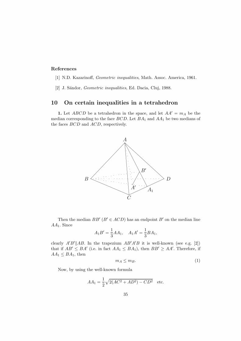
1. Let ABCD be a tetrahedron in the space, and let AA′ = mA be themedian corresponding to the face BCD. Let BA1 and AA1 be two medians ofthe faces BCD and ACD, respectively.

A

B

C

A1

D

B′

A′

Then the median BB′ (B′ ∈ ACD) has an endpoint B′ on the median lineAA1. Since

A1B′ =

1

3AA1, A1A

′ =1

3BA1,

clearly A′B′‖AB. In the trapezium AB′A′B it is well-known (see e.g. [2])that if AB′ ≤ BA′ (i.e. in fact AA1 ≤ BA1), then BB′ ≥ AA′. Therefore, ifAA1 ≤ BA1, then

mA ≤ mB . (1)

Now, by using the well-known formula

AA1 =1

2

√2(AC2 +AD2) − CD2 etc.

35

clearly AA1 ≤ BB1 will be equivalent to

AC2 +AD2 ≤ BC2 +BD2. (2)

On other words, if (2) is valid, then (1) is valid, too, i.e. mA ≤ mB. But(2) is in fact a characterization for mA ≤ mB. Indeed, it is well-known (andfollows from the above figure) that

9AA′2 = 3(AB2 +AC2 +AD2) − (BC2 + CD2 +BD2) (3)

9BB′2 = 3(BA2 +BC2 +BD2) − (AC2 + CD2 +AD2)

AA′ ≤ BB′ ⇔ AC2 +AD2 ≤ BC2 +BD2.

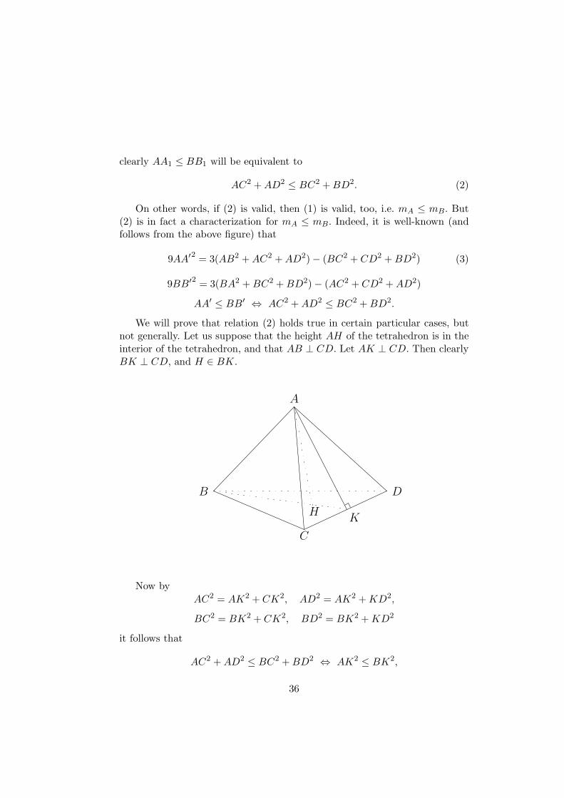
We will prove that relation (2) holds true in certain particular cases, butnot generally. Let us suppose that the height AH of the tetrahedron is in theinterior of the tetrahedron, and that AB ⊥ CD. Let AK ⊥ CD. Then clearlyBK ⊥ CD, and H ∈ BK.

A

B

C

K

D

H

Now by

AC2 = AK2 + CK2, AD2 = AK2 +KD2,

BC2 = BK2 + CK2, BD2 = BK2 +KD2

it follows that

AC2 +AD2 ≤ BC2 +BD2 ⇔ AK2 ≤ BK2,

36

i.e. AK ≤ BK. Now since

SA = area(BCD) = BK · CD/2, SB = area(ACD) = AK · CD/2,

clearlyAK ≤ BK ⇔ SB ≤ SA.

Therefore, we have proved that in such tetrahedron one has:

mA ≤ mB ⇔ SB ≤ SA. (4)

By repeating the argument to other faces, relation (4) and its analogousrelations give the following result: If ABCD is orthocentric, having acute-angled faces, then

mA ≤ minmB ,mC ,mD ⇔ SA ≥ maxSB , SC , SD. (5)

This is a strengthening of a particular case of OQ.1324 by M. Olteanu [1].However, (5) is not true in all tetrahedrons! It is sufficient to show that (2) isnot generally true (with SB ≤ SA). In fact this can be rewritten as

AC2 + CD2 +AD2 ≤ BC2 + CD2 +BD2 ⇔ SB ≤ SA.

Now, in a general triangle having side lengths a, b, c it is well known that

16S2 = 2∑

a2b2 −∑

a4.

Since (∑a2)2

=∑

a4 + 2∑

a2b2,

and denoting∑

a2 = k we get

16S2 + k2 = 4∑

a2b2 = 4c2(a2 + b2) + 4a2b2 = 4c2k + 4a2b2 − 4c4.

Thus16S2 = −k2 + 4c2k + 4a2b2 − 4c2 := f(k). (6)

The function f(k) (k > 0) has a maximum attained at kmax = 2c2. Clearly,if 0 < k < kmax, then f(k) is strictly increasing, while for k ≥ kmax, f(k) isstrictly decreasing. So, for 0 < k1, k2 ≤ 2c2, k1 ≤ k2 ⇒ f(k1) ≤ f(k2).Remark that k ≤ 2c2 means that a2 + b2 + c2 ≤ 2c2, i.e. a2 + b2 ≤ c2 (i.e. theangle C in the triangle is obtuse). Thus when the triangle ACD, BCD arenot acute-angled (in A and B), the relation doesn’t hold.

37

A

B

C

DT

S

M

R

u

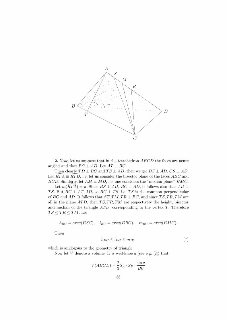
2. Now, let us suppose that in the tetrahedron ABCD the faces are acuteangled and that BC ⊥ AD. Let AT ⊥ BC.

Then clearly TD ⊥ BC and TS ⊥ AD, then we get BS ⊥ AD, CS ⊥ AD.Let RTA ≡ RTD, i.e. let us consider the bisector plane of the faces ABC andBCD. Similarly, let AM ≡MD, i.e. one considers the ”median plane” BMC.

Let m(RTA) = u. Since BS ⊥ AD, BC ⊥ AD, it follows also that AD ⊥TS. But BC ⊥ AT,AD, so BC ⊥ TS, i.e. TS is the common perpendicularof BC and AD. It follows that ST, TM,TR ⊥ BC, and since TS, TR, TM areall in the plane ATD, then TS, TR, TM are respectively the height, bisectorand median of the triangle ATD, corresponding to the vertex T . ThereforeTS ≤ TR ≤ TM . Let

hBC = area(BSC), lBC = area(BRC), mBC = area(BMC).

Then

hBC ≤ lBC ≤ mBC (7)

which is analogous to the geometry of triangle.Now let V denote a volume. It is well-known (see e.g. [2]) that

V (ABCD) =2

3SA · SD · sinu

BC

38

(where SA = area(BCD)). By decomposing the tretrahedron in two smallertetrahedrons, it follows that

2

3·SD · lBC · sin u

2BC

+2

3·SA · lBC · sin u

2BC

=2

3·SA · SD · 2 sin

u

2cos

u

2BC

one gets

lBC =2SA · SD

SA + SD· cos u

2. (8)

But

V =hBC ·AD

3=

2

3SA · SD · sinu

BC,

so

hBC =2

3· SA · SD · sinu

BC. (9)

Since lBC ≥ hBC , (8) and (9) imply the inequality

SA + SD ≤ BC ·AD2 sin

u

2

=Σ

sinu

2

(10)

where Σ is the area of a triangle with base BC and height AD. Note thatrelation (10) is the extension to the space of the triangle inequality

b+ c ≤ a

sinA

2

(11)

see ([3], Lemma 1). For other inequalities in a tetrahedron, see [2].

References

[1] M. Olteanu, OQ.1324, Octogon Math. Mag., 11(2003), no.2, 859.


[3] J. Sandor, On Emmerich’s inequality, Octogon Math. Mag., 9(2001),no.2, 861-864.

39

11 Certain trigonometric inequalities deduced byconvexity methods

Trigonometric inequalities are important in many fields of Mathemat-ics (Elementary geometry, Mathematical analysis, Fourier series, Numerical

analysis, etc.). While the inequalities like sinx < x, tg x > x, x ∈(0,π

2

)are

well-known, many similar inequalities, like Jordan’s inequality sinx >2

πx are

rediscovered from time to time. For example, in a recent note [1] this, and the

inequality tgx

2<

2

πx are proved by using certain auxiliary functions. However,

this way doesn’t suggest a method of discovery of such inequalities.In what follows we shall employ the convexity method to deduce simple

(and in many cases important in applications), trigonometric inequalities.

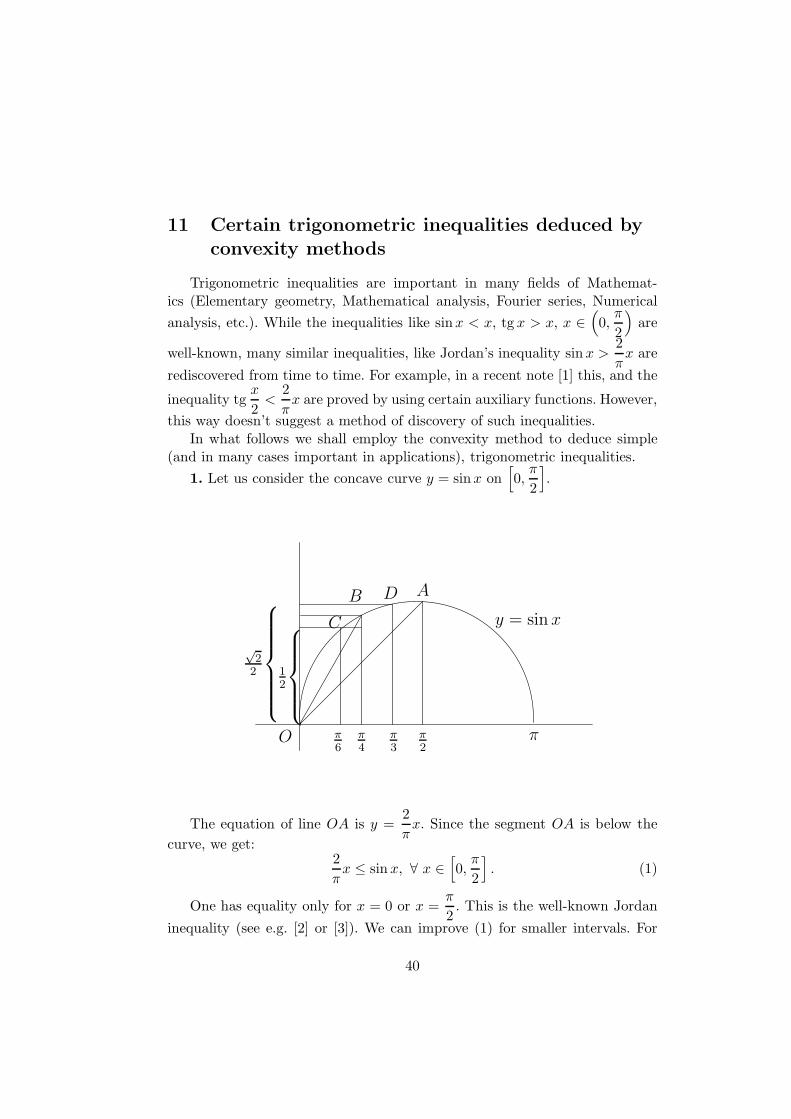
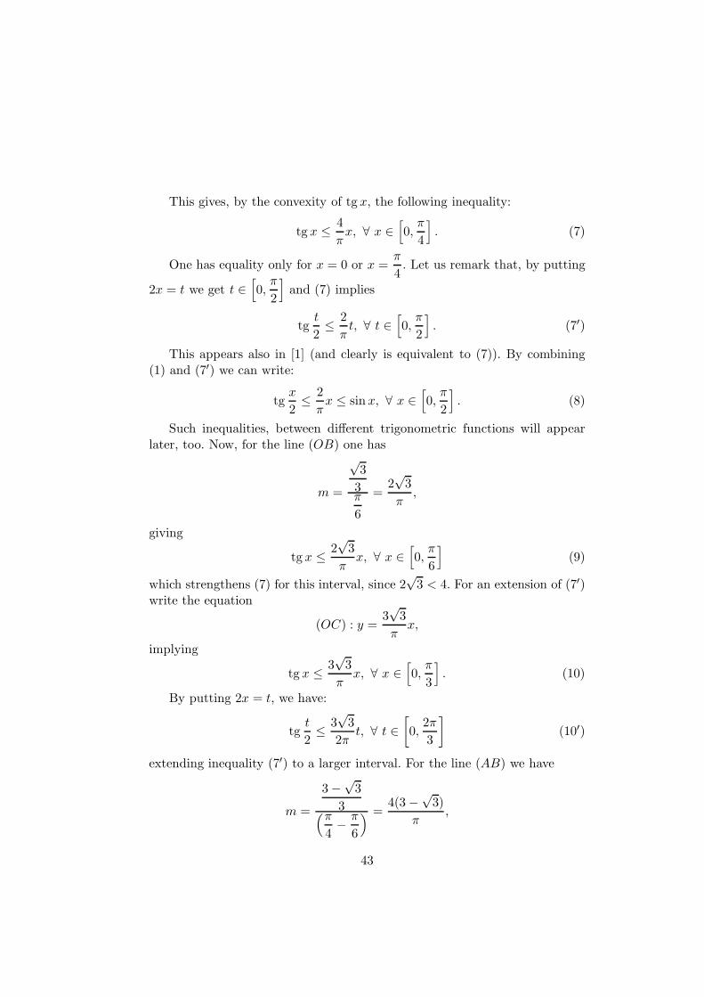
1. Let us consider the concave curve y = sinx on[0,π

2

].

A

O ππ2

π3

π4

π6

B

C

D

12

√2

2

y = sin x

The equation of line OA is y =2

πx. Since the segment OA is below the

curve, we get:2

πx ≤ sinx, ∀ x ∈

[0,π

2

]. (1)

One has equality only for x = 0 or x =π

2. This is the well-known Jordan

inequality (see e.g. [2] or [3]). We can improve (1) for smaller intervals. For

40

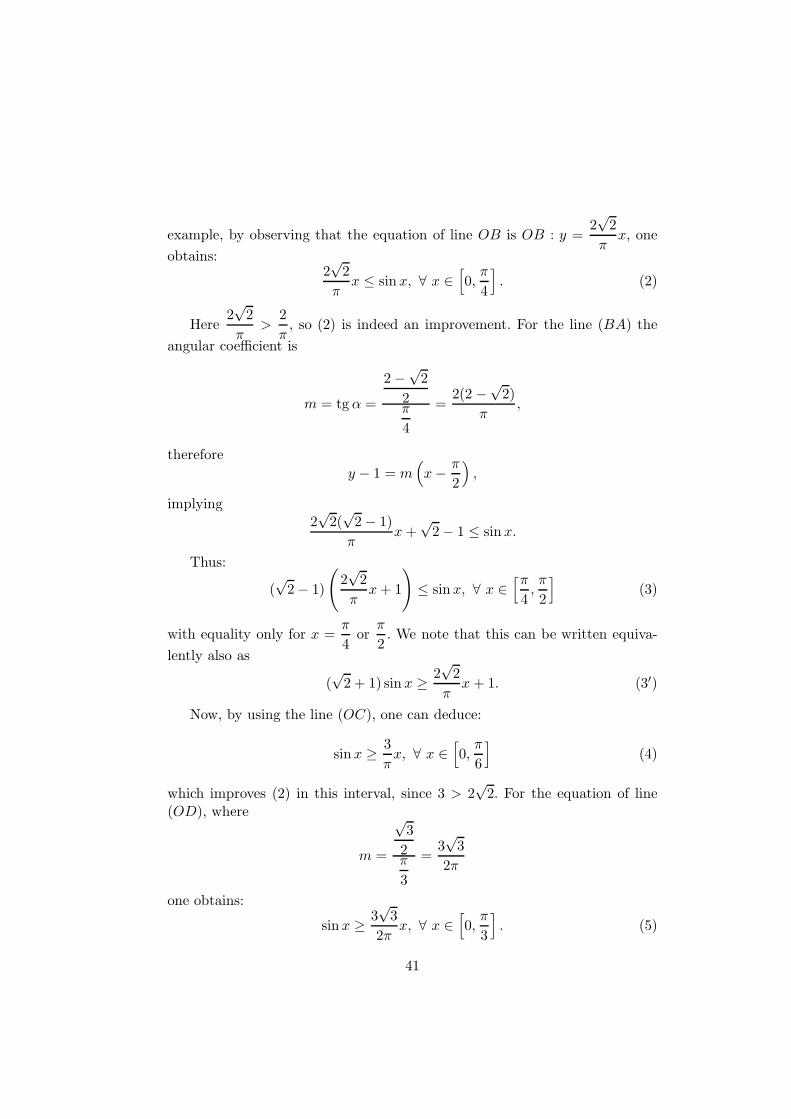
example, by observing that the equation of line OB is OB : y =2√

2

πx, one

obtains:2√

2


[0,π

4

]. (2)

Here2√

2

π>

2

π, so (2) is indeed an improvement. For the line (BA) the

angular coefficient is

m = tg α =

2 −√

2

2π

4

=2(2 −

√2)

π,

therefore

y − 1 = m(x− π

2

),

implying2√

2(√

2 − 1)

πx+

√2 − 1 ≤ sinx.

Thus:

(√

2 − 1)

(2√

2

πx+ 1

)≤ sinx, ∀ x ∈

[π4,π

2

](3)

with equality only for x =π

4or

π

2. We note that this can be written equiva-

lently also as

(√

2 + 1) sin x ≥ 2√

2

πx+ 1. (3′)

Now, by using the line (OC), one can deduce:

sinx ≥ 3

πx, ∀ x ∈

[0,π

6

](4)

which improves (2) in this interval, since 3 > 2√

2. For the equation of line(OD), where

m =

√3

2π

3

=3√

3

2π

one obtains:

sinx ≥ 3√

3

2πx, ∀ x ∈

[0,π

3

]. (5)

41

For the line (CB) one has

m =

√2 − 1

2π

12

=6(√

2 − 1)

π,

therefore

y − 1

2=

6(√

2 − 1)

π

(x− π

6

),

giving:

sinx ≥ 6(√

2 − 1)

π

(x− π

6

)+

1

2

for x in[π6,π

4

]. This can be transformed, after certain elementary computa-

tions, to

(√

2 + 1) sinx ≥ 6

πx+

√2 − 1

2, ∀ x ∈

[π6,π

4

]. (6)

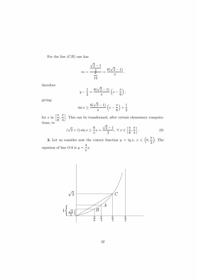
2. Let us consider now the convex function y = tg x, x ∈(0,π

2

). The

equation of line OA is y =4

πx.

π2

π3

π4

π6

√3 C

AB√

33

1

42

This gives, by the convexity of tg x, the following inequality:

tg x ≤ 4

πx, ∀ x ∈

[0,π

4

]. (7)

One has equality only for x = 0 or x =π

4. Let us remark that, by putting

2x = t we get t ∈[0,π

2

]and (7) implies

tgt

2≤ 2

πt, ∀ t ∈

[0,π

2

]. (7′)

This appears also in [1] (and clearly is equivalent to (7)). By combining(1) and (7′) we can write:

tgx

2≤ 2


[0,π

2

]. (8)

Such inequalities, between different trigonometric functions will appearlater, too. Now, for the line (OB) one has

m =

√3

3π

6

=2√

3

π,

giving

tg x ≤ 2√

3

πx, ∀ x ∈

[0,π

6

](9)

which strengthens (7) for this interval, since 2√

3 < 4. For an extension of (7′)write the equation

(OC) : y =3√

3

πx,

implying

tg x ≤ 3√

3

πx, ∀ x ∈

[0,π

3

]. (10)

By putting 2x = t, we have:

tgt

2≤ 3

√3

2πt, ∀ t ∈

[0,

2π

3

](10′)

extending inequality (7′) to a larger interval. For the line (AB) we have

m =

3 −√

3

3(π4− π

6

) =4(3 −

√3)

π,

43

so

y − 1 =4(3 −

√3)

π

(x− π

4

),

yielding

tg x ≤ 4(3 −√

3)

πx+

√3 − 2, ∀ x ∈

[π4,π

6

]. (11)

This can be written also in the form:

(3 +√

3)tg x ≤ 24

πx− (3 −

√3), ∀ x ∈

[π4,π

6

]. (11′)

3. In the preceding two paragraphs we have deduced inequalities for thesin and tg functions. We now remark that these can be easily transformed

into inequalities for the cos and ctg functions. Applying e.g. (1) for x =π

2− y

(y ∈

[0,π

2

])one obtains:

cos y ≥ 1 − 2

πy, ∀ y ∈

[0,π

2

], (12)

known also as Kober’s inequality.

In the same manner from (2), since x ∈[0,π

4

]gives y ∈

[π4,π

2

], we get:

cos y ≥√

2 − 2√

2

πy, ∀ y ∈

[π4,π

2

]. (13)

Analogously, from (4) we get

cos y ≥ 3

2− 3

πy, ∀ y ∈

[π3,π

2

](14)

while from (3′) we can obtain:

(√

2 + 1) cos y ≥√

2 + 1 − 2√

2

πy, ∀ y ∈

[0,π

2

](15)

or in an equivalent form

cos y ≥ 1 − 2

π(2 −

√2)y, ∀ y ∈

[0,π

4

]. (15′)

We note that this improves (12) since 2 −√

2 < 1. Now, inequality (7)

applied to x =π

2− y yields

ctg y ≤ 2 − 4

πy, ∀ y ∈

[π4,π

2

]. (16)

44

In the same manner, from (10) one can prove

ctg y ≤ 3√

3

2− 3

√3

πy, ∀ y ∈

[π6,π

2

]. (17)

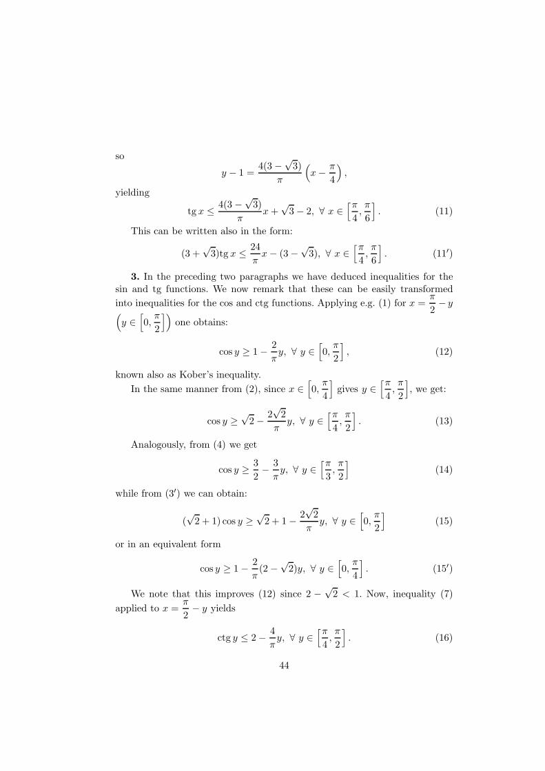
4. We now use tangent lines to concave or convex curves.

(0, 1)

(π4, 0) (

π2, 0)

Writing the tangent equation to the curve y = cos x at the point(π

2, 0)

since (cos x)′ = − sinx, we have y− 0 = −1(x− π

2

). Since the curve is below

the tangent, we get

cosx ≤ π

2− x, ∀ x ∈

[0,π

2

](18)

with equality only for x = 0 or x =π

2. Before going further, we give an

application of Jordan’s inequality, combined with (18). By

tg x =sinx

cos x>

2

πx

π

2− x

=4

π· x

π − 2x,

we get Steckin’s inequality (see [2])

tg x >4

π· x

π − 2x, ∀ x ∈

(0,π

2

). (19)

45

For another proof, see [3]. By writing the tangent line equation at the point(π

4,

√2

2

)to the graph of y = cos x, by the same method we can deduce:

cos x ≤ π − 2√

2

4−

√2

2x, ∀ x ∈

[0,π

2

]. (20)

Remark that (15′) and (20) written in a single line, give:

1 − 2

π(2 −

√2)x ≤ cosx ≤ π − 2

√2

4−

√2

2x, x ∈

[0,π

4

]. (21)

By writing the tangent lines to the curve y = sinx at D

(π

3,

√3

2

),

y =

√3

2+

1

2

(x− π

3

),

we get:

sinx ≤ x

2+

√3

2− π

6, ∀ x ∈ [0, π]. (22)

By writing the tangent line to the convex curve y = tg x at A(π

4, 1)

since

(tg x)′ =1

cos2 x, we get y − 1 = 2

(x− π

4

), implying

tg x ≥ 2x− π

2+ 1, ∀ x ∈

(0,π

2

)(23)

with equality only for x =π

4. We note here that (23) and (19) cannot be

compared (i.e. one of them doesn’t imply the other one for all x).5. The above methods can be applied to inverse trigonometrical functions,

too. Considering e.g. the concave curve y = arctg x on [0,∞) one obtains easily

arctg x ≥ π

4x, ∀ x ∈ [0, 1]. (24)

By writing the tangent line equation in the point(1,π

4

), by (arctg x)′ =

1

1 + x2, one obtains y − π

4=

1

2(x− 1), giving

arctg x ≤ x− 1

2+π

4, ∀ x ∈ [0,∞). (25)

46

For the convex curve y = arcsin x, x ∈ [0, 1] by writing the line passing on

(0, 0) and(1,π

2

), we get

arcsinx ≤ π

2x, ∀ x ∈ [0, 1] (26)

while by writing the tangent line equation at

(√2

2,π

4

)we get

arcsinx ≥√

2x+π

4− 1, ∀ x ∈ [0, 1]. (27)

More generally (and this can be done in all cases) for an arbitrary x0 ∈(0, 1) one can obtain

arcsinx ≥ arcsin x0 +x− x0√1 − x2

0

, ∀ x ∈ [0, 1]. (28)

6. Another argument is to approximate sin or cos by a quadratic function.

Let us consider f(x) = ax(π − x). Since f ′(0) = πa, we will select a =1

π.

Then f ′(π) = −1 as for the sin function. Now it is immediate that the graphof f is below the graph of sin on [0, π], giving:

sinx ≥ x(π − x)

π, ∀ x ∈ [0, π]. (29)

Such simple inequalities have importance in Fourier series. Remark thatx(π − x)

π≥ 2x

π⇔ π − x ≥ 2 i.e. x ≤ π − 2 (π − 2 <

π

2by π < 4). Thus for

x ∈ [0, π − 2], relation (29) is better than Jordan’s inequality (1). Applyingthe same procedure to the cos function and

f(x) = −a(x− π

2

)(x+

π

2

), a > 0,

since (cos x)′x= π

2= −1, we select a =

1

π, and as above one can deduce the

inequality

cos x ≥ − 1

πx2 +

π

4, ∀ x ∈

[−π

2,π

2

](30)

The functions sin and cos can be approximated by more complicated functions,too.

For example, by taking

f(x) = x

(π2 − x2

π2 + x2

),

47

one can deduce Redheffer’s inequality (see [2] or [3])

sinx

x≥ π2 − x2

π2 + x2, ∀ x ∈ [0, π]. (31)

By considering

f(x) = x

(πa − xa

πa + xa

) 1a

,

inequalities of type(

sinx

x

)a

≤ πa − xa

πa + xa, ∀ x ∈

[0,π

2

](32)

can be proved, see [4].7. Finally, we apply the well-known Jensen-Hadamard (or Hermite-

Hadamard, or Hadamard) inequalities for concave (or convex) functions f :[a, b] → R (see e.g. [5]):

(b− a)

[f(a) + f(b)

2

]≤

(<)

∫ b

af(x)dx ≤

(<)(b− a)f

(a+ b

2

). (33)

Let f(x) = cos x, [a, b] = [0, t] with f strictly concave. Then (33) implies

1 + cos t

2<

sin t

t< cos

t

2, ∀ t ∈

(0,π

2

]. (34)

For f(x) = sinx one can deduce

sin t

2<

1 − cos t

t< sin

t

2, ∀ t ∈

(0,π

2

]. (35)

For an application of (34), let us assume that t ≥ π

3. Then the cos function

being decreasing, one has

cost

2≤ cos

π

6=

√3

2.

Therefore1 + cos t

2<

sin t

t<

√3

2for t ∈

[π3,π

2

]. (36)

The relationsin t

t<

√3

2is complementary to

sin t

t>

2

π. Finally, let f(x) =

tg x on [a, b] = [0, t], t ∈(0,π

2

]. Since f is convex and

∫ t

0tg xdx = − ln(cos t),

we get the relation:

tgt

2<

− ln(cos t)

t< tg t, ∀ t ∈

(0,π

2

). (37)

48

For various selections of t one can compare this inequality to the existingrelations, but we conclude here. Other inequalities, like Huygens’

2 sin x+ tg x < 2x, x ∈(0,π

2

)

can be found in [3].

References

[1] M. Bencze, Inequalities in the triangle, Octogon Math. Mag., 7(1999),no.1, 99-107.

[2] D.S. Mitrinovic, Analytic inequalities, Springer Verlag, 1970.


[4] J. Sandor, On the open problem OQ.532, Octogon Math. Mag., 9(2001),1B, 569-570.

[5] J. Sandor, On the Jensen-Hadamard inequality, Studia Univ. Babes-Bolyai, 36(1991), 9-15.

12 On some trigonometric inequalities of Bencze

M. Bencze posed in [1] as open question OQ.1216, proof of the inequality

cos

(1

2

n∑

k=1

xk

)≤ n

n∑

k=1

xk

sinxk

(1)

where xk ∈(0,π

2

), k = 1, 2, . . . , n, n ≥ 1. W. Janous [3] settled this question

in three steps.(i) Inequality (1) is false whenever n ≥ 7. Indeed, let

x1 = · · · = xn =4π

n.

Then for n ≥ 9 we have4π

n∈(0,π

2

)and (1) becomes

4π

n≤ sin

4π

nin

contradiction to the inequality sinx < x valid for all x > 0. For n = 7 and

49

n = 8, we let x1 = · · · = xn =π

2− t where t > 0 and t → 0. Then (1) reads

cos(n

2

(π2− t))

≤sin(π

2− t)

π

2− t

.

Now t = 0 yields for n = 7 and n = 8 the two invalid inequalities

√2

2≤ 2

π

and 1 ≤ 2

π, resp. Therefore a continuity-argument shows that (1) cannot be

true in general.

(ii) For n = 1 inequality (1) becomes cos(x

2

)≤ sinx

x, that is

x

2≤ sin

x

2.

This shows that (1) is false for n = 1, too.(iii) On the other hand, for n = 2, 3, 4, 5, 6 inequality (1) is true. In order

to prove this assertion we employ a special case of a general majorizationinequality, namely: If we suppose that m ≤ xi ≤ M , i = 1, . . . , n then thereexists a unique w ∈ [m,M) and a unique integer N ∈ 0, 1, . . . , n such that:

n∑

i=1

xi = (n−N − 1)m+ w +NM.

Then for any convex function f : [m,M ] → R it holds

n∑

i=1

f(xi) ≤ (n−N − 1)f(m) + f(w) +Nf(M) (2)

(see [2], p.64 and 132). Now, it is well-known that

f(x) =x

sinx, 0 ≤ x ≤ π

2,

is convex.Now the proof of the five mentioned cases of n runs as follows:

Let e.g. n = 5. Then x1, . . . , x5 ∈(0,π

2

)yields for x1 + · · ·+x5 = N

π

2+w,

0 ≤ w <π

2the five subcases N = 0, 1, 2, 3, 4 with the corresponding five

inequalities

cos

(Nπ

4+w

2

)≤ 5

4 −N +Nπ

2+

w

sinw

, 0 ≤ w <π

2. (3)

50

(In order to estimate the sums5∑

k=1

xk

sinxkwe employ inequality (2) and

limx→0

x

sinx= 1.) Now (3) is immediate for N = 2, 3, 4 as its left-hand side

is negative.The cases N = 0 and N = 1 are checked by a computer-algebra system as

are the respective inequalities for the remaining cases of n. We summarize theabove considerations as:

Theorem. Inequality (1) is valid if n ∈ 2, 3, 4, 5, 6.Remark. Inequalities (3) for N = 0 and general n ∈ N deserve special

attention. They read

cosw

2≤ n sinw

w + (n− 1) sinw,

that is

w + (n− 1) sinw ≤ 2n sinw

2, (4)

where 0 ≤ w ≤ π

2.

We claim that (4) is valid whenever n ≥ 2 even for 0 ≤ w ≤ π. Indeed, ifwe let

f(w) = 2 sinw

2− (n− 1) sinw − w,

then

f ′(w) = n cosw

2− (n− 1) cosw − 1 = −2(n− 1) cos2 w

2+ n cos

w

2+ n− 2

=(1 − cos

w

2

)(2(n− 1) cos

w

2+ n− 2

),

whence f ′(w) ≥ 0. This and f(0) = 0 yields the claim. Furthermore, as f(w),

0 ≤ w ≤ 3π

2, firstly increases and then decreases we get due to

f

(3π

2

)= n(

√2 + 1) − 3π

2− 1 :

Inequality (4) is valid for 0 ≤ w ≤ wn, where wn >3π

2, when = even

n ≥ 3.

51

References

[1] M. Bencze, OQ.1216-1218, Octogon Math. Mag., 11(2003), no.1, 390.

[2] A.W. Marshall, I. Olkin, Inequalities - Theory of Majorization and itsapplications, Academic Press, New York, 1979.

[3] W. Janous, On some trigonometric inequalities of M. Bencze, OctogonMath. Mag., 11(2003), no.2, 720-724.

13 Onsin x

x

We will determine all a ∈ R such that(

sinx

x

)a

≤ πa − xa

πa + xafor all x ∈

(0,π

2

). (1)

We may assume a > 0 since for a ≤ 0 clearly πa − xa < 0. Then (1) canbe written also as

sinx ≤ f(x) = x

(πa − xa

πa + xa

) 1a

(2)

where we extend the definition of f to [0, π]. After certain elementary compu-tations one can deduce that the derivative f is

f ′(x) =

(πa − xa

πa + xa

) 1a

(−x2a − 2πaxa + π2a

π2a − x2a

). (3)

Since by putting πa = λ, xa = t, the quadratic equation −t2−2λt+ t2 = 0has the solutions t1 = λ(

√2 − 1), t2 = −λ(

√2 + 1), one can deduce that the

numerator of the second term in (3) can be decomposed as [πa(√

2 − 1) −xa][πa(

√2 + 1) + xa]. Therefore we have obtained that f(0) = 0, f(π) = 0

and f has a maximum at x0 =π√

2 + 1(= π(

√2 − 1)). To prove that (2)

holds true we must show that f(π

2

)≥ 1 (since

π√2 + 1

<π

2and otherwise

there exists x1 ∈(0,π

2

)with sinx1 > f(x1) - contradiction). The inequality

f(π

2

)≥ 1 becomes equivalent with

(2a − 1

2a + 1

) 1a

≥ π

2, a > 0. Since the function

g : (0,∞) → R, g(a) =

(2a − 1

2a + 1

) 1a

is strictly increasing (which can be easily

52

shown with the derivative of log g) and lima→∞

g(a) = 1, there exists a single

a0 > 0 such that g(a0) =2

π< 1. Here a0 > 1, otherwise g(a0) ≤ g(1) =

1

3, i.e.

2

π≤ 1

3(6 ≤ π) - contradiction. Any a ≥ a0 satisfies inequality (1). We note

that a0 < 2, since for a0 ≥ 2 we would obtain g(a0) ≥√

3

4, i.e. 16 ≥ 3π2 -

contradiction.Remark. Since a = 2 is a solution of (1), by Redheffer’s inequality ([1],

[2])sinx

x≥ π2 − x2

π2 + x2we can write the following double inequality:

(sinx

x

)2

≤ π2 − x2

π2 + x2≤ sinx

x, x ∈

(0,π

2

). (4)

References

[1] D.S. Mitronovic, Analytic inequalities, Springer Verlag, 1970.


14 On de Cusa’s trigonometric inequality

According to F.T. Campan ([1]) the following trigonometric inequality wasdiscovered by Nicolaus de Cusa (1401-1464):

Theorem 1. For all x ∈(0,π

2

)one has

3 sin x

2 + cos x< x.

Such inequalities (along with e.g. 2 sinx + tg x > 3x, known as Huygens’inequality, see e.g. [1], [2]) were studied by geometric arguments also by Wille-brod Snellius (1581-1626), and Christian Huygens (1629-1695).

We shall extend de Cusa’s inequality as follows:Theorem 2. Let a, b, c > 0 such that 3b ≤ c ≤ a + b. Then for any

x ∈(0,π

2

)one has

c sin x

a+ b cos x< x.

53

Proof. Let us consider the application f :[0,π

2

)→ R,

f(x) = x(a+ b cos x) − c sinx.

One can remark that f(0) = 0,

f ′(x) = a+ b cos x− bx sinx− c cos x, f ′(0) = a+ b− c ≥ 0

by assumption. Moreover,

f ′′(x) = (sinx)(c − 2b) − bx cos x = (cos x)[(c− 2b)tg x− bx].

Put g(x) = (c − 2b)tg x − bx, x ∈[0,π

2

). By g(0) = 0, g′(x) =

(c− 2b) − b cos2 x

cos2 x, since b cos2 x− (c− 2b) ≤ b− (c− 2b) = 3b− c ≤ 0 we get

g′(x) ≥ 0, i.e. g is an increasing function. Thus g(x) > g(0) for x > 0. This inturn implies f ′′(x) > 0, so f ′(x) > f ′(0) ≥ 0 for x > 0, i.e. f ′(x) > 0. Thusf(x) > f(0) = 0 for x > 0, and this finishes the proof of the theorem.

Remark. For a = 2, b = 1, c = 3 we reobtain Theorem 1.

References

[1] F.T. Campan, The story (fairy tale) of the number π (Romanian), Ed.Albatros, Romania, 1977.


15 A property of sin1

x

We will determine a class of functions f : R∗+ → R∗

+ so that f(x) → 0(x → ∞) and x2[f(x) − f(x + 1)] → 1 (x → ∞). An example is given by

f(x) = sin1

x.

Theorem. If f is differentiable and x2f ′(x) → l (x→ ∞), then x2[f(x)−f(x+ 1)] → −l.

Proof. By the Lagrange mean-value theorem we can write

f(x) − f(x+ 1) = [x− (x+ 1)]f ′(ξ),

where x < ξ < x+1. Byx

ξ< 1 <

x

ξ+

1

ξ, we get ξ → ∞ and

x

ξ→ 1 as x→ ∞.

Now,

x2[f(x) − f(x+ 1)] = −x2f ′(ξ) = −(x

ξ

)2

(ξ2f ′(ξ)) → −1 · l = −l,

54

by the given assumption. This proves the theorem.

Remark 1. For f(x) = sin1

xone has x2f ′(x) = − cos

1

x→ −1 as x→ ∞,

so x2[f(x) − f(x+ 1)] → 1.Remark 2. The above result (in Remark 1) could be deduced also by the

L’Hopital rule.

16 (sinx)cosx + (cosx)sinx made integer

Let A = (sinx)cos x + (cos x)sin x ∈ Z.First note that we must suppose sinx > 0, cosx > 0. Then clearly

0 < (sinx)cos x ≤ 1, 0 < (cos x)sin x ≤ 1.

Thus 0 < A ≤ 2. On the other hand, A has the form A = ab + ba, wherea, b > 0. It is well-known that ab + ba > 1 for all a, b > 0 (see e.g. [1], p.281).Since A is integer, this implies A ≥ 2. Therefore, we must have A = 2, i.e.

(sinx)cos x = 1, (cos x)sin x = 1.

This implies sinx = cos x = 1, which is impossible. Therefore A 6∈ Z, forall x ∈ R.

References


55

56

Chapter 2

Sequences and series of realnumbers

”... The infinite we shall do right away. The finite may take a little longer.”

(Stanislaw M. Ulam)

”... Mathematics is concerned only with the enumeration and comparisonof relations.”

(Carl F. Gauss)

57

1 On certain limits related to the number e

1. In the very interesting web pages by Steven Finch ([3]) there appearsalso the following limit, submitted by Felix A. Keller:

limn→∞

[nn

(n− 1)n−1− (n− 1)n−1

(n− 2)n−2

]= e. (1)

In what follows we will show how certain expressions which are similarto the bracket in (1), are intimately related to certain special means of twoarguments, namely the logarithmic and identric means.

Let a, b > 0 be two positive real numbers. The logarithmic, resp. identricmeans of a and b are defined by

L = L(a, b) =b− a

ln b− ln a(a 6= b), L(a, a) = a

and

I = I(a, b) =1

e(bb/aa)1/(b−a) (a/neb), I(a, a) = a.

For many properties, generalizations, etc. of these means we quote e.g. [1],[2], [5], [8], [10].

The following inequalities, which will be used here, are due to K.B. Sto-larsky [10]:

√ab < L(a, b) < I(a, b) <

a+ b

2(a 6= b). (2)

These relations can be much improved, see e.g. [8].2. In what follows, we will use the following notations:

f(x) =

(1 +

1

x

)x

, F (x) = (x+ 1)

(1 +

1

x

)x

,

g(x) = ln

(1 +

1

x

)− 1

x+ 1(x > 0).

Since ln I(x, x+ 1) = (x+ 1) ln(x+ 1) − x lnx− 1 and

1

L(x, x+ 1)= ln(x+ 1) − lnx, (3)

we easily can see that

ln(F (x)) = ln(x+ 1) + ln f(x) = ln eI(x, x+ 1),

58

so

F (x) = eI(x, x+ 1) = (x+ 1)f(x) (4)

and

F ′(x) =F (x)

L(x, x+ 1)(5)

where F ′ denotes the derivative of F .3. We note that by (3) we have

f(x) =e

xI(x, x+ 1),

so by inequalities (2) applied to a := x, b := x + 1, we get the followingdouble-inequality

e

√x

x+ 1< f(x) < e

2x+ 1

2x+ 2. (6)

As a consequence, we can write

x√x+

√x+ 1

e < x[e− f(x)] <x

2x+ 2e, (7)

yielding the following limit:

limx→∞

x[e− f(x)] =e

2. (8)

Of course, this limit may be obtained by l’Hopital rule, too. However, theinequalities provide a much better information. For another proof of (7), basedon Hadamard’s inequality, see [7].

Remark. By

nf(n)− (n − 1)f(n − 1) = n[f(n)− e] + (n− 1)[e− f(n− 1)] + e,

(8) implies

limn→∞

[nf(n)− (n− 1)f(n− 1)] = e (8′)

proved by other arguments in [6]. The limit (8′) is due to M. Ghermanescu [4].4. We now prove first the following result:Theorem 1. For x > 0, F is a strictly increasing, strictly concave func-

tion.Proof. Clearly,

F ′(x) =F (x)

L(x, x+ 1)> 0,

59

and, on the other hand since

F ′′(x) = F (x)

[(ln(x+ 1) − lnx)2 − 1

x(x+ 1)

]

= F (x)

[1

L2(x, x+ 1)− 1

x(x+ 1)

],

by the left side of (2) we clearly get F ′′(x) < 0. Thus F is strictly concave.Corollary 1. For all positive integers n > 1 one has

f(n)2n

2n+ 1< F (n + 1) − F (n) < f(n− 1)

√n

n+ 1. (9)

Proof. By Lagrange’s mean value theorem one has

F (n+ 1) − F (n) = F ′(ξ) (ξ ∈ (n, n+ 1)),

and by Theorem 1, F ′ is strictly decreasing, so we have

F (n + 1)

L(n+ 1, n + 2)< F (n+ 1) − F (n) <

F (n)

L(n, n+ 1). (10)

Now, (9) follows by (10) and (2), by remarking that

F (n) = (n+ 1)f(n)

and2n

2n+ 1<

n

L(n, n+ 1)<

√n

n+ 1.

Corollary 2. limn→∞

[F (n+ 1) − F (n)] = e. (11)

This follows from (10), or (9), if we remark that f(n) → e (n → ∞). Thusthe limit (1) follows.

Remark. Clearly, (9)-(10) are valid for all positive real numbers n > 1.5. The bracket in limit (1) can be written also as

nf(n− 1) − (n− 1)f(n− 2) = n[f(n− 1) − f(n− 2)] + f(n− 2).

Since f(n− 2) → e (n→ ∞), we clearly get (from (1) or (11) that

limn→∞

n[f(n− 1) − f(n− 2)] = 0. (12)

60

This could be proved also by l’Hopital rule, but we are interested for moreprecise relations of type (6), or (9), (10). These in turn allow us to studyinteresting problems.

Theorem 2. The function g is strictly positive, strictly decreasing forx > 0, and all x > 0, the following inequality is valid:

(g(x))2 + g′(x) < 0. (13)

Proof. Since

g(x) =1

L(x, x+ 1)− 1

x+ 1,

the inequality g(x) > 0 is a simple consequence of the fact that L is a mean(or the right-side of (2)). A simple computation shows that

g′(x) =−1

x(x+ 1)2< 0.

In order to prove (13), calculate

(g(x))2 + g′(x) =

[1

L(x, x+ 1)− 1

x+ 1

]− 1

x(x+ 1)2< 0 ⇔

1

L(x, x+ 1)− 1

x+ 1<

1

(x+ 1)√x

⇔

L(x, x+ 1) >(x+ 1)

√x√

x+ 1.

This is true, since L(x, x+1) >√x(x+ 1) (see (2)) it is sufficient to prove

that √x(x+ 1) >

(x+ 1)√x√

x+ 1,

or equivalently√x+ 1 >

√x+ 1.

Corollary 3. The function f is strictly increasing and strictly concave forall x > 0.

Proof. Since

f ′(x) = f(x)g(x), f ′′(x) = f(x)[g(x)]2 + g′(x),

this is a simple consequence of Theorem 2 (i.e. (13)).Corollary 4. Let (an) be a strictly positive sequence such that

limn→∞

ang(n) = l. (14)

61

Thenlim

n→∞an[f(n) − f(n− 1)] = le. (15)

Proof. By the Lagrange mean-value theorem one has

f(n) − f(n− 1) = f ′(ξ) = f(ξ)g(ξ),

and since f is strictly concave, fg is strictly decreasing, yielding the doubleinequality

f(n)g(n) < f(n) − f(n− 1) < f(n− 1)g(n − 1) (n > 1). (16)

Now (15) follows from (16), (14), and the remark that

limn→∞

g(n − 1)g(n) = 1

(this is implied by (2), but also by simple application of l’Hopital rule).Examples. 1) Let an = n. Then ang(n) → 0 (more generally, xg(x) → 0

as x→ ∞), so from (15) we reobtain (12).

2) Let an = n2. Then, since x2g(x) → 1

2(x→ ∞), we obtain

limn→∞

n2[f(n) − f(n− 1)] =e

2. (17)

Remark. This limit is due to Gh. Stoica [9].6. Since f is strictly concave, we have that the sequence (f(n+ 1)− f(n))

is strictly decreasing. Similarly, the sequence (F (n + 1) − F (n)) is strictlydecreasing, too. We consider the sequence given by the limit (8).

Theorem 3. Let h(x) = f(x)[1 + xg(x)] (x > 0). Then the function h isstrictly increasing.

Proof. Since f ′(x) = f(x)g(x), after a simple calculus we get

h′(x) = f(x)[2g(x) + x(g2(x) + g′(x))]. (18)

Since g(x) =1

L− 1

x+ 1(where L = L(x, x + 1) for simplified notation),

the square bracket in (18) is

P (y) = xy2 + 2y − 1

(x+ 1)2,

where

y =1

L− 1

x+ 1.

62

Since the roots of the polynomial P (y) are

y1,2 =−(x+ 1) ±

√x+ (x+ 1)2

x(x+ 1)

it is sufficient to prove that

1

L− 1

x+ 1>

√x+ (x+ 1)2 − (x+ 1)

x(x+ 1),

or

L <x(x+ 1)√

x+ (x+ 1)2 − 1. (19)

We shall use (see (2)) the inequality L <2x+ 1

2and prove that

2x+ 1

2<

x(x+ 1)√x+ (x+ 1)2 − 1

. (20)

After certain easy (but tedious) computations, this becomes equivalent to0 < 3x2 + x, and this finishes the proof of the theorem.

Corollary 5. Let u(x) = x[e−f(x)]. Then u is a strictly increasing concavefunction.

Proof. u′(x) = e− f(x)(1 + xg(x)) < 0, since f(x)(1 + xg(x)) = h(x) < eby theorem 3 and the fact that lim

x→∞h(x) = e. By u′′(x) = −h′(x) < 0, we get

that u is concave.Corollary 6. For all n > 1 we havea) 2nf(n) < (n− 1)f(n− 1) + (n+ 1)f(n+ 1)b) 2(n + 1)f(n) > nf(n− 1) + (n+ 2)f(n + 1)c) 2f(n) > f(n− 1) + f(n+ 1).Proof. Since u is strictly concave, we have

u(n+ 1) − u(n) < u(n) − u(n− 1),

which transforms into a).On the other hand, by Theorem 1, F (x) = (x+ 1)f(x) is strictly concave,

too, thus

F (n+ 1) − F (n) < F (n) − F (n− 1),

giving b). Finally, relation c) is a consequence of Corollary 2 (i.e., the functionf is strictly concave).

63

References

[1] H. Alzer, Ungleichungen fur Mittelwerte, Arch. Math., 47(1986), 422-426.

[2] B.C. Carlson, The logarithmic mean, Amer. Math. Monthly, 79 (1972),615-618.

[3] S. Finch, Favorite mathematical constants. The number e, Seehttp://www/mathsoft.com/asolve/constant/constant.html.

[4] M. Ghermanescu, Problem 4600, Gaz. Mat., 41(1935), 216.

[5] A.O. Pittenger, Inequalities between arithmetic and logarithmic means,Univ. Beograd Publ. Elektr. Fak. Ser. Mat. Fiz., 680(1980), 15-18.

[6] T. Popoviciu, On the calculation of certain limits (Romanian), Gaz. Mat.Ser. A, vol.LXXVI, no.1, 1971, 8-11.

[7] J. Sandor, On Hadamard’s inequality (Hungarian), Mat. Lapok, 87(1982), 427-430.

[8] J. Sandor, On the identric and logarithmic means, Aequationes Math.,40(1990), 261-270.

[9] Gh. Stoica, Problem C:325, Gaz. Mat. 8/1983, 358.

[10] K.B. Stolarsky, The power and generalized logarithmic means, Amer.Math. Monthly, 87(1980), 545-548.

Note added in proof. After completing this paper we have learned thatProfessors H. Brothers and J.A. Knox have proved relation (1) by using certainseries expansions for e. The author is grateful to the authors for calling hisattention to the following papers: 1) H.J. Brothers and J.A. Knox, New closedform approximations to the logarithmic constant e, Mathematical Intelligencer20(1998), no.4, 25-29; 2) H.J. Brothers and J.A. Knox, Novel series-basedapproximations to e, College Math. Journal, vol.30, 1999, 269-275.

2 On some strange sequences

A.

Let (un) be a sequence defined by(

1 +1

n

)n+un

= e, n = 1, 2, . . . (1)

64

Then

un =1

ln

(1 +

1

n

) − n.

Put1

n= t, and consider

f(t) =1

ln(1 + t)− 1

t=t− ln(1 + t)

t ln(1 + t).

Since

ln(1 + t) = t− t2

2+t3

3− . . . ,

one has

f(t) =

t2

2− t3

3+t4

4− . . .

t2 − t3

2+t4

3− . . .

=

1

2− t

3+t2

4− . . .

1 − 1

2+t2

3− . . .

= a0 + a1t+ a2t2 + . . .

Then

(1 − t

2+t2

3− . . .

)(a0 + a1t+ a2t

2 + . . . ) =1

2− t

3+t2

4− . . .

Let the power series (obtained by Cauchy-product) on the left side be∞∑

n=1

cntn. Then clearly

cn = an − 1

2an−1 +

1

3an−2 − · · · + (−1)n−1 a1

n+

(−1)na0

n+ 1= (−1)n

1

n+ 2(2)

by identification. Since a0 =1

2, c0 =

1

2, we get successively

c1 = a1 −1

2a0 = −1

3,

so

a1 =1

4− 1

3= − 1

12, c2 = a2 −

1

2a1 +

1

3a0 =

1

4,

so

a2 =1

4− 1

24− 1

6=

1

24, . . .

65

We have obtained

un =1

2+ a1

1

n+ a2

1

n2+ . . . , (3)

where all (ai) are recurrently determined by (2). Thus un → 1

2(n → ∞)

and (3) gives the asymptotical development. The sequence (xn) defined byx2n+1 = un, x2n = un − 1 in OQ.805 therefore cannot be convergent.

Application. We will determine a, b ∈ R, so that

na

(un − 1

2

)→ b as n→ ∞ (see [1]) (1)

In a recent note [2] we have determined the asymptotic expansion of thesequence (un), given by

un =1

2+a1

n+a2

n2+ . . . (2)

where a1, a2, . . . are constants (which can be effectively computed). Now (2)implies

n

(un − 1

2

)→ a1 = − 1

12. (3)

Therefore, as an answer to the problem (1), the following can be stated:

if a = 1, then b = a1. If a > 1, then b = −∞. Since un − 1

2→ 0, clearly for

a ≤ 0 one has b = 0. For a ∈ (0, 1) from (3) it follows that b = 0.

References

[1] M. Bencze, D. M. Batinetu-Giurgiu, OQ.1023, Octogon Math. Mag.,10(2002), no.2, 1052.

[2] J. Sandor, On the Open Problem OQ.805, Octogon Math. Mag., 10(2002), no.1, 416.

B.

Let (xn) be a sequence defined by

[1

e

(1 +

1

n

)n]n+xn

=1√e

(1)

66

By taking logarithms, one obtains

(n+ xn)

[−1 + n ln

(1 +

1

n

)]= −1

2,

thus

xn =1

2

[1 − n ln

(1 +

1

n

)] − n. (2)

Put t =1

n, and consider the expression

1

2

[1 − 1

tln(1 + t)

] − 1

t=

t− 2 +2

tln(1 + t)

2t

[1 − 1

tln(1 + t)

] = A.

Since

ln(1 + t) = t− t2

2+t3

3− . . .

we get

A =

t− 2 +2

t

(t− t2

2+t3

3− . . .

)

2t

[1 − 1

t

(t− t2

2+t3

3− . . .

)] =t− 2 + 2 − t+

2

3t2 − t3

2+ . . .

2t− 2t+ t2 − 2

3t3 +

t4

2− . . .

=

2

3t2 − t3

2+ . . .

t2 − 2

3t3 +

t4

2− . . .

=2

3+ a1t+ a2t

2 + . . . ,

where the coefficient ai (i = 1, 2, . . . ) can be determined from the equality

2

3t2 − t3

2+ · · · =

(t2 − 2

3t3 +

t4

2− . . .

)(2

3+ a1t+ a2t

2 + . . .

). (3)

For this method, based on Cauchy-product of series, see our note [2]. Thusa1, a2, . . . , can be effectively computed (e.g. a1 = −1/18). All in all, the as-ymptotical expansion of xn is

xn =2

3+ a1

1

n+ a2

1

n2+ . . . (4)

Particularly, limn→∞ xn =2

3, answering OQ.863 of [1].

67

References

[1] M. Bencze, OQ.863, Octogon Math. Mag., 10(2002), no.1, 518.


C.

Let (xn) be determined by

n

((1 +

1

n

)−n+xn

− 1

e

)

=1

2e. (1)

An easy computation gives

xn =

ln

(1 +

1

2n

)− 1

ln

(1 +

1

n

) + n. (2)

Put1

n= x, and consider the expression

A =ln(1 +

x

2

)− 1

ln(1 + x)+

1

x=x ln

(1 +

x

2

)− x+ 1

x ln(1 + x)

=

x2

2− x3

2 · 22+

x4

3 · 23− x5

4 · 24+ · · · − x+ x− x2

2+x3

3− x4

4+ . . .

x2

(1 − x

2+x2

3− x3

4+ . . .

)

=

5

24x3 − 5

24x4 +

59

320x5 − . . .

x2

(1 − x

2+x2

3− x3

4+ . . .

) =

x

(5

24− 5

24x+

59

320x2 − . . .

)

1 − x

2+x2

3− x3

4+ . . .

= B

where we have used the following well-known formulae:

ln(1 + x) = x− x2

2+x3

3− . . .

ln(1 +

x

2

)=x

2− x2

2 · 22+

x3

3 · 23− . . .

68

for x in a neighborhood of 0. Now B can be written as

B = x(a0 + a1x+ a2x2 + . . . ),

where a0, a1, a2, . . . can be determined by considering the Cauchy product ofpower series (see [2]):

(a0 + a1x+ a2x2 + . . . )

(1 − x

2+x2

3− x3

4+ . . .

)=

5

24− 5

24x+

59

320x2 − . . .

For example, a0 =5

24, a1 = − 5

48, . . . Therefore,

xn =1

n

(a0 +

a1

n+a2

n2+ . . .

), (3)

implying e.g. that

xn → 0 (4)

nxn → a0 =5

24etc. (5)

References



D.

Let (xn) be a sequence defined by the relation:

1

n+

1

n+ 1+ · · · + 1

2n= logxn

(2n+ 1

n

). (1)

Since

logxn

(2n+ 1

n

)=

ln

(2n+ 1

n

)

lnxn,

clearly

lnxn =

ln

(2 +

1

n

)

c2n − cn, (2)

69

where

cn = 1 +1

2+ · · · + 1

n. (3)

Since cn = lnn + γ + o(1), it is well-known that c2n − cn = ln 2 + o(1).Then (2) implies

xn → e (n→ ∞) (4)

Now, by Taylor expansion it is immediate that

ln

(2 +

1

n

)= ln 2 +

1

n· 1

1 · 2 − 1

n2· 1

2 · 22+

1

n3· 1

3 · 23− . . . (5)

On the other hand, it is well-known that (and this can be deduced e.g. bythe Euler-Maclaurin summation formula)

cn = 1 +1

2+ · · · + 1

n= γ + lnn+

1

2n+ α1

1

n2+ α2

1

n4+ . . . (6)

(where in fact α1 = −B1

2, α2 =

B2

4, . . . with (Bi) the Bernoulli numbers), we

get

c2n − cn =1

n+ 1+ · · ·+ 1

2n= ln 2 + b1

1

n+ b2

1

n2+ . . . (b1 = −1

4, etc.). (7)

Now, by (2)

lnxn =ln 2 + a1x+ a2x

2 + . . .

ln 2 + b1x+ b2x2 + . . .= 1 + c1x+ c2x

2 + . . . (8)

(where x =1

n) (where (ai) are from (5), while (bi) from (7)). Now (ci) can be

determined by the Cauchy-product of two series and a simple recurrence (forthis method see [1]).

References

[1] J. Sandor, On the open problem OQ.805, Octogon Math. Mag., 10(2002),no.1, 416.

E.

Let (xn) be determined by the relation

(n

en

)n+xn

= n!, (1)

70

where en =

(1 +

1

n

)n

.

By logarithmation we get

xn =lnn!

lnn− n ln

(1 +

1

n

) − n. (2)

Since

lnn! =

(n+

1

2

)lnn− n+ a0 +

a1

n+a2

n2+ . . . (Stirling series)

and

ln

(1 +

1

n

)=

1

n− 1

2n2+

1

3n3− . . .

from (2) we can write, after a short computation:

xn =

1

2lnn+ c0 +

c1n

+c2n2

+ . . .

lnn+ a0 +a1

n+a2

n2+ . . .

(3)

Here all coefficients are known (e.g. a0 = 1, c0 = ln√

2π− 1

2, etc.). There-

fore, from (3) xn can be computed with as higher accuracy as we wish. Forexample, (3) implies

xn =1

2+

A

lnn+O

(1

n lnn

)(4)

implying also xn → 1

2(n → ∞),

(xn − 1

2

)lnn→ A (n → ∞), etc.

F.

Let (xn) be a sequence given by

1 +1

2+ · · · + 1

n− ln(n+ xn) = γ,

where γ is Euler’s constant. We will prove that limn→∞

xn =1

2, and will find

the asymptotical evaluation of (xn). The result with limn→∞

xn =1

2as for as

71

we know, was proposed also as a problem in Gazeta Matematica (Bucuresti).Here we obtain a new solution. De Tempe [1] gave an elementary proof that:

1

24(n + 1)2<

n∑

k=1

1

k− ln

(n+

1

2

)− γ <

1

24n2. (1)

This gives the double inequality(n+

1

2

)e

124(n+1)2 − n < xn <

(n+

1

2

)e

124n2 − n. (2)

Now, it is not difficult to prove (e.g. with l’Hopital rule) that each side

of (2) has a limit equal to1

2as n → ∞. This proves that (xn) is convergent,

having as a limit1

2.

Negoi [2] has applied De Tempe’s method to prove that

− 1

48n3<

n∑

k=1

1

k− ln

(n+

1

2+

1

24n

)− γ < − 1

48(n + 1)3(3)

so(n+

1

2+

1

24n

)e−

148n3 − n < xn <

(n+

1

2+

1

24n

)e− 1

48(n+1)3 − n. (4)

Tims and Tyrell [3] proved in 1971 that

1 − log en <

n∑

k=1

1

k− log n− γ < 1 − log en−1 for n ≥ 2 (5)

where en =

(1 +

1

n

)n

. This implies

e

en< 1 +

xn

n<

e

en−1, (6)

or written equivalently

n(e− en)

en< xn <

n(e− en−1)

en−1. (7)

Now, Brother and Knox [4] (see also [5]) deduced

en = e

(1 − 1

2n+

11

2n2− 7

16b3+ . . .

), (8)

72

so one can again reobtain the above result on xn (by en → e, en−1 → e). Now(4) gives

limn→∞

n

(xn − 1

2

)=

1

24. (9)

By the repetition of De Tempe’s method, clearly follows

xn =1

2+a1

n+a2

n2+ . . . (10)

where a1, a2, . . . are constant (e.g. a1 =1

24). However this could be obtained

also by the Euler-Maclaurin summation formula, as well.

References

[1] D.W. De Tempe, A quicker convergence to Euler’s constant, Amer.Math. Monthly, 100(1993), 468-470.

[2] T. Negoi, A faster convergence to Euler’s constant, Gazeta Matematica(Romanian), no.15/1997, 111-113.

[3] S.R. Tims, J.A. Tyrrel, Approximate evaluation of Euler’s constant,Math. Gaz. LV, 391(1971), 65-67.

[4] H.J. Brothers, J.A. Knox, New closed-form approximations to the loga-rithmic constant e, Math. Intelligencer, 20(1998), no.4, 25-29.

[5] J. Sandor, On OQ.666, Octogon Math. Mag., 9(2001), no.2, 961.

Application. Let the general term if the sequence (xn) be defined by asabove. Determine a, b ∈ R, such that

na

[n

(xn − 1

2

)− 1

24

]→ b (n→ ∞). (1′)

In the note [1] the asymptotic expansion of xn is written as

xn =1

2+a1

n+a2

n2+ . . . (2′)

where a1 =1

24, a2, . . . are constants.

Therefore, on base of (2’) one can write

n

[n

(xn − 1

2

)− 1

24

]= a2 +

a3

n+ . . . ,

73

so i.e.

n

[n

(xn − 1

2

)− 1

24

]→ a2 as n→ ∞. (3′)

Now, if a ≤ 0, since n

(xn − 1

2

)− 1

24→ 0, clearly b = 0. For a ∈ (0, 1),

on base of (3’) the limit in (1’) is true for b = 0.If a > 1, then (3’) implies b = ∞.

References

[1] J. Sandor, On the Open Problem OQ.804, Octogon Math. Mag., 10(2002), no.1, 414-415.

G.

Let (xn) be determined by

(1 +

xn

n

)n= 1 +

1

1!+

1

2!+ · · · + 1

n!.

We will prove here that the sequence (xn) is convergent, having limn→∞

xn =

1. Put

sn =1

1!+

1

2!+ · · · + 1

n!.

Since (1 +

1

n

)n

= 1 +1

1!+

1

2!

(1 − 1

n

)+ · · ·+

+1

k!

(1 − 1

n

)(1 − 2

n

). . .

(1 − k − 1

n

)+ · · ·+

+1

n!

(1 − 1

n

)(1 − 2

n

). . .

(1 − n− 1

n

)

> 1 +1

1!+

1

2!

(1 − 1

n

)+ · · · + 1

k!

(1 − 1

n

)(1 − 2

n

). . .

(1 − k − 1

n

)

for k < n. Let now be k fixed and n → ∞ in the above relation. One getssk ≤ e.

On the other hand,

(1 +

1

k

)k

= 1 +1

1!+

1

2!

(1 − 1

k

)+ · · ·+

74

+1

k!

(1 − 1

k

). . .

(1 − k − 1

k

)≤ 1 +

1

1!+

1

2!+ · · · + 1

k!= sk.

Therefore, the following double-inequality has been proved:

(1 +

1

k

)k

≤ 1 +1

1!+ · · · + 1

k!≤ e. (1)

This gives

1 ≤ k

[k

√1 +

1

1!+ · · · + 1

k!− 1 . . .

]≤ k( k

√e− 1) (2)

which means that:

1 ≤ xk ≤ e1/k − 1

1/k. (3)

Since limx→∞

ex − 1

x= 1, clearly lim

k→∞e1/k − 1

1/k= 1, so on base of (3) one

gets: limk→∞

xk = 1.

Remark. Since (sk) is strictly increasing and sk → e, in fact one hassk < e (k = 1, 2, . . . ) in (1).

References

[1] M. Bencze, OQ.811, Octogon Math. Mag., 10(2002), no.1, p.506.

[2] J. Sandor, On the Open Problem OQ.811, Octogon Math. Mag., 11(2003), 225.

H.

Let (xn) given by the relation

(1 +

1

n+ xn

)n

=1

2e. (1)

It is required to prove that (xn) is convergent, as well as to give the as-ymptotical expansion of xn (see [1]).

Pute

2= k. Then k > 1, ln k < 1 as

e

2< e. (1) gives

xn =1

k1n − 1

− n. (2)

75

Put1

n= x and consider

A =1

kx − 1− 1

x=x+ 1 − kx

x(kx − 1).

By using the Maclaurin expansion of kx, one has

kx = 1 +ln k

1!x+

(ln k)2

2!x2 + . . .

Put a = ln k, a ∈ (0, 1). Then

A =

x+ 1 −(

1 +a

1!x+

a2

2!x2 + . . .

)

x

(a

1!x+

a2

2!x2 + . . .

)

=1 − a− a2

2!x− a3

3!x2 − . . .

x

(a

1!+a2

2!x+

a3

3!x2 + . . .

) =1

x(a0 + a1x+ a2x

2 + . . . )

where a0, a1, a2, . . . can be determined by

(a

1!+a2

2!x+

a3

3!x2 + . . .

)(a0 + a1x+ a2x

2 + . . . ) = 1− a− a2

2!x− a3

3!x2 − . . .

(using Cauchy products, see e.g. [2]). For example, a0 =1 − a

a, a1 = −1

2, etc.

Therefore,

xn = n

(1 − a

a− 1

2· 1

n+ a2

1

n2+ . . .

). (3)

This implies

xn − n

(1 − a

a

)→ −1

2as n→ ∞, (4)

so, as1 − a

a> 0, this implies

xn → ∞. (5)

76

References




I.

Let (xn) be defined by

− ln(2n+ xn) +

2n∑

k=1

1

k= γ. (1)

Put

xn =

2n∑

k=1

1

k− ln(2n) − γ. (2)

Then cn → 0 (n→ ∞), as it is well-known. The xn given by (1) and (2) isin fact:

xn = 2n(ecn − 1). (3)

Now, sinceecn − 1

cn→ 1, xn = (2ncn)yn, where yn = (ecn − 1)/cn; so we

must study the limit of (2ncn). Put 2n = m. We will show that:

mcm → 1

2(m→ ∞). (4)

We shall apply the Cesaro-Stolz theorem for the case0

0(see [1]). By

cm+1 − cm1

m+ 1− 1

m

=

[1

m+ 1− ln

(1 +

1

m

)]− (m(m+ 1));

and

ln

(1 +

1

m

)=

1

m− 1

2m2+O

(1

m3

),

and1

m+ 1− 1

m+

1

2m2=

−m+ 1

2m2(m+ 1),

77

one has−m(m+ 1)(−m+ 1)

2m2(m+ 1)→ 1

2as m→ ∞,

so (4) follows. Thus

limn→∞

xn =1

2. (5)

Regarding the asymptotic expansion of (xn), this may be obtained by theknown asymptotic development of

cm =1

2m+ α1

1

m2+ α2

1

m4+ . . .

(where α1 = −B1

2, α2 =

B2

4, . . . with Bernoulli numbers (Bi)), and from

m(ecm − 1) = m

(cm1!

+c2m2!

+ . . .

)(6)

since

c2m =1

4m2+a1

m3+ . . .

We successively get

m(ecm − 1) =1

2+

1

8· 1

m+ b1

1

m2+ b2

1

m3+ . . . ,

where the constants b1, b2, . . . can be determined inductively. By replacingm = 2n, we get the asymptotic expansion of (xn):

xn =1

2+

1

16· 1

n+ b′1

1

n2+ b′2

1

n3+ . . . (7)

References

[1] G. Garnir, Fonctions de variables reelles, Gauthier Villars, Paris, Tome1, 1963.

[2] J. Sandor, On the Open Problem OQ.1048, Octogon Math. Mag.,11(2003), no.1, 260-261.

78

J.

Letn∑

k=1

1

k= lnn+ γ +

60n3 − 10n2 + xn

120n4,

where γ is Euler’s constant. Prove that (xn) is convergent and determine theasymptotical expansion of (xn).

This follows at once from the well-known expansion of Hn =

n∑

k=1

1

k(see

e.g. [2])

Hn = γ + lnn+1

2n+ α1

1

n2+ α2

1

n4+ α3

1

n6+ . . . (1)

(where in fact α1 = −B2

2, α2 =

B2

4, . . . with (Bi) the Bernoulli numbers).

This immediately implies

xn = 120α2 +120α3

n2+ . . . (2)

implying

xn → 120α2,

and giving of course the expansion of (xn) (see [3]).

References




K.

Let

xn =

2n∑

k=1

1

n+ k.

We will determine in what follows

limn→∞

n2(exn+1 − exn).

79

Let cn =

n∑

k=1

1

k. Then

xn = c2n − cn = (c3n − ln 3n) − (cn − lnn) + ln 3 → γ − γ + ln 3 = ln 3

(where γ is Euler’s constant). Thus:

limn→∞

xn = ln 3. (1)

Remark thatxn+1 = xn + kn (2)

where

kn =1

3n+ 1+

1

3n+ 2− 2

3(n + 1). (3)

Thus n2(exn+1−exn) = n2exn(ekn−1). Here kn → 0, and sinceekn − 1

kn→ 1

(known limit), limn→∞

n2(exn+1 − exn) = 3 limn→∞

n2kn (by (1)). Remark that

kn =1

3n+ 1+

1

3n + 2− 2

3(n + 1)

=(3n+ 2)(3n + 2) + (3n + 1)(3n + 3) − 2(3n + 1)(3n + 2)

(3n + 1)(3n + 2)(3n + 3)

=9n + 5

(3n+ 1)(3n + 2)(3n + 3).

Thus n2kn → 9

27=

1

3, i.e.

limn→∞

n2(exn+1 − exn) = 1. (4)

L.

Let (yn) be defined by (see [1])

logyn

(3n+ 1

n

)=

n∑

k=1

1√1 + (n + k)2

. (1)

Put

un =n∑

k=1

1√1 + k2

− ln(n +√n2 + 1).

80

It is known that (un) is convergent, un → u (u→ ∞). Thus

n∑

k=1

1√1 + (n+ k)2

= u2n + ln(2n +√

4n2 + 1) − (un + ln(n+√n2 + 1))

= u2n − un + ln2n+

√4n2 + 1

n+√n2 + 1

→ u− u+ ln4

2= ln 2 (as n→ ∞).

Since by (1) one has

yn =

(3n+ 1

n

)1/nP

k=1

1√1+(n+k)2 → 3

1ln 2 as n→ ∞

(see [2]).

References

[1] D.M. Batinetu-Giurgiu, OQ.1082, Octogon Math. Mag., 10(2002), no.1,1066.

[2] J. Sandor, On OQ.1082 and OQ.1083, Octogon Math. Mag., 11(2003),no.1, 269.

M.

Let

Bk =(k + 1)2

k+1√

(k + 1)!− k2

k√k!

and Ln = n+1√

(n + 1)! − n√n!.

It is well-known that Ln → 1

2(n → ∞) and Bn → e (n → ∞). In [1] the

limit

limn→∞

1

n

n∑

k=1

(Γ(1 +Bk))Bk+Lk (1)

is required. We shall use the following result:

an → a ⇒ a1 + a2 + · · · + an

n→ a (n→ ∞). (2)

Since an = (Γ(1 + Bn))Bn+Ln → (γ(1 + e))e+1e (Γ being a continuous

functions), this last value is the value of the limit in expression C1.

81

Remark. In a similar manner,

limn→∞

1

n

n∑

k=1

(Γ(1 +Bk))1/Bk = (Γ(1 + e))1/e,

answering OQ.998, by the same author (see p.1046 of this journal).

References


[2] J. Sandor, On OQ.999, Octogon Math. Mag., 11(2003), 253.

N.

Let

xn =

n∑

k=1

(−1)k+1

2k − 1.

Reference [1] asks certain questions related to limn→∞

n(π

4− xn

). We will

show that this limit doesn’t exist! First remark that

x2m = 1 − 1

3+

1

5− · · · − 1

4m− 1, x2m+2 = x2m +

1

4m+ 1− 1

4m+ 3.

Thus(π

4− x2m+2

)−(π

4− x2m

)

1

2m+ 2− 1

2m

=2

(4m+ 1)(4m + 3)

(−2m(2m+ 2)

2

)

→ 1

4as m→ ∞.

The0

0case of the Stolz-Cesaro theorem implies that

limn→∞

2m(π

4− x2m

)=

1

4. (1)

Now, in a similar manner, one can write

x2m+1 = 1 − 1

3+

1

5+ · · · + 1

4m+ 1, x2m−1 = 1 − 1

3+ · · · + 1

4m− 3,

82

so

x2m+1 − x2m−1 = − 1

4m− 1+

1

4m+ 1=

−2

(4m− 1)(4m + 1).

Thus

π

4− x2m+1 −

(π4− x2m−1

)

1

2m+ 1− 1

2m− 1

=−(2m+ 1)(2m − 1)

2· 2

(4m− 1)(4m+ 1)

→ −1

4as m→ ∞.

Thus

limm→∞

(2m− 1)(π

4− x2m−1

)= −1

4. (2)

By combining (1) and (2) one can say that indeed limn→∞

n(π

4− xn

)doesn’t

exist.

References



O.

Let (Gn) be the Ghermanescu sequence, defined by (see [2])

Gn =(n+ 2)n+1

(n+ 1)n− (n+ 1)n

nn−1. (1)

It is well-known thatGn → e as n→ ∞. (2)

In [1] the following limit appears as an Open Question:

limn→∞

1

n

n∑

k=1

(Γ(1 +Gk))1/Gk (3)

where Γ is Euler’s gamma function. We shall use the fact that if an → a, then

a1 + a2 + · · · + an

n→ a (n→ ∞). (4)

83

Now, an = (Γ(1+Gn))1/Gn → (Γ(1+e))1/e, since Γ is a continuous function.Therefore, the limit in (3) is (Γ(1 + e))1/e.

Remark. For various other limits, related to number e, see our paper [2],

where among others appears also that the function e(x) =

(1 +

1

x

)x

(x > 0)

is strictly increasing and strictly concave.

References


[2] J. Sandor, On certain limits related to the number e, Libertas Mathe-matica, 20(2000), 155-159.

P.

Let

Gn =(n + 2)n+1

(n + 1)n− (n + 1)n

nn−1, n ≥ 1

be the Ghermanescu sequence.Let

f(n) =

(1 +

1

n

)n

.

ThenGn = (n + 1)f(n+ 1) − nf(n)

= (n + 1)[f(n + 1) − e] + n[e− f(n)] + e = xn − xn+1 + e,

where xn = n[e− f(n)]. This sequence appears also in [3], [4]. Now, by usingMathematica Program, H.J. Brothers and J.A. Knox [2] has obtained thefollowing expansion:

(1 +

1

x

)x

= e

[1 − 1

2x+

11

24x2− 7

16x3+

2447

5760x4− 959

2304x5+ . . .

]. (1)

By putting x = n and n+ 1, from (1), we get:

Gn = e+11e

24· 1

n(n+ 1)− 7e

16· 2n+ 1

n2(n+ 1)2+

2447e

5760· 3n2 + 3n+ 1

n3(n+ 1)3− . . . (2)

By using this expansion, the following interesting limits can be deduced:

limn→∞

n2(Gn − e) =11e

24(3)

84

limn→∞

n3

[Gn − e− 11e

24n2

]= −7e

8, etc. (4)

References

[1] D.M. Batinetu-Giurgiu, OQ.666, Octogon Math. Mag., 9(2001), no.1B,689.

[2] H.J. Brothers, J.A. Knox, New closed-form approximations to the loga-rithmic constant e, Mathematical Intelligencer, 20(1998), no.4, 25-29.

[3] J. Sandor, On certain limits related to the number e, Libertas Mathe-matica, 20(2000), 155-159.

[4] J. Sandor, L. Debnath, On certain inequalities involving the constant eand their applications, J. Math. Anal. Appl., 249(2000), 569-582.

Q.

Let

xn =

n∑

k=1

Γ′(Lk) − Γ(Ln),

where Ln = n+1√

(n+ 1)! − n√n!, n = 1, 2, . . . and Γ is the Euler’s gamma

function.We will show that the sequence (xn) is divergent.Indeed,

xn+1 − xn = Γ′(Ln+1) − Γ(Ln+1) + Γ(Ln).

Since, it is well-known that Ln → 1

eand Γ and Γ′ are continuous functions

on (0,∞), the right side of the above expression has a limit

Γ′(

1

e

)− Γ

(1

e

)+ Γ

(1

e

)= Γ′

(1

e

).

Clearly, Γ′(

1

e

)6= 0. If xn → a ∈ R (n → ∞), then 0 = a− a = Γ′

(1

e

),

which is impossible.Indeed, since Γ is strictly increasing, Γ′ has a single zero on (0,∞), namely

between 1 and 2, since Γ(2)−Γ(1) = Γ′(ξ) (by Lagrange mean value theorem),

so 1 − 1 = 0 = Γ′(ξ) with ξ ∈ (1, 2). But1

e< 1, so ξ 6= 1

e.

85

R.

Let

b = limn→∞

(n∑

k=1

tg1

k− lnn

),

and the sequence (xn) defined by

ln(n+ xn) =

n∑

k=1

tg1

k− b. (1)

We will show that the sequence (xn) is convergent. Put

bn =n∑

k=1

tg1

k− lnn,

for simplicity. Relation (1) gives:

xn = eln n+bn−b − n = n(ebn−b − 1). (2)

Since bn − b→ 0 andebn−b − 1

bn − b→ 1 (n→ ∞), by (2)

xn = n(bn − b)yn (3)

where yn = (ebn−b−1)/(bn−b), so we must show the convergence of (n(bn−b)).We shall use the Stolz-Cesaro lemma for the case

0

0(see e.g. [1]), by remarking

that n(bn − b) =bn − b

1

n

. Here

(bn+1 − b) − (bn − b)1

n+ 1− 1

n

= −n(n+ 1)(bn+1 − bn)

= −n(n+ 1)

(tg

1

n+ 1− ln

(1 +

1

n

)). (4)

By using l’Hopital rule (or the expansion

tg x =x

1!+

2x3

3!+ · · · + ln(1 + x) = x− x2

2+ . . . )

it can be shown that the limit of expansion (4) is1

2. Therefore (xn) is conver-

gent, and

limn→∞

xn =1

2. (5)

86

References

[1] H.G. Garnir, Fonctions de variables reelles, Gauthier Villars, Paris, I,1963.

S.

Let

bn =

n∑

k=1

tg1

k− lnn− b, cn =

n∑

k=1

1

k− lnn− γ,

d =n∑

k=1

sin1

k− lnn− d,

where γ is Euler’s constant, while

b = limn→∞

(n∑

k=1

tg1

k− lnn

), d = lim

n→∞

(n∑

k=1

sin1

k− lnn

).

In another note [3] we have proved that:

nbn → 1

2(n→ ∞). (1)

In a completely similar manner, it follows that:

ncn → 1

2(n→ ∞) (2)

ndn → 1

2(n→ ∞). (3)

Now, in OQ.1062 one has

xn = n2(ecn+bn − 1) (4)

while in OQ.1063,xn = n2(ebn+dn − 1) (5)

and in OQ.1064,xn = n3(ecn+bn+dn − 1). (6)

Sinceecn+bn − 1

cn + bn→ 0, etc., we must calculate lim

n→∞n2(cn+bn), lim

n→∞n2(bn+

dn), limn→∞

n3(cn+bn+dn). By (1), (2), (3) clearly all these limits have the value

+∞.

87

References

[1] D.M. Batinetu-Giurgiu, M. Bencze, OQ.1962, OQ.1063, Octogon Math.Mag., 10(2002), no.2, 1062.


[3] J. Sandor, On the Open Problem OQ.1061, Octogon Math. Mag.,11(2003), no.1, 264-265.

T.

Put

bn =

n∑

k=1

tg1

k− lnn, cn =

n∑

k=1

1

k− lnn, dn =

n∑

k=1

sin1

k− lnn.

It is known that the sequences (bn), (cn), (dn) are convergent. Now, letbn → b, cn → γ, dn → d (n→ ∞). Then

n∑

k=1

tg1

n+ k= b2n + ln 2n− (bn + lnn)

= b2n − bn + ln 2 → b− b+ ln 2 = ln 2, as n→ ∞.

Similarly:n∑

k=1

sin1

n+ k→ ln 2 and

n∑

k=1

1

n+ k→ ln 2 as n→ ∞.

Now, in OQ.1042 [1], a sequence (xn) is defined by

logxn

3n+ 1

n=

n∑

k=1

(1

n+ k+ sin

1

n+ k+ tg

1

n+ k

)(1)

so

xn =

(3n+ 1

2

)1/nP

k=1( 1

n+k+sin 1

n+k+tg 1

n+k)

(2)

since

3n+ 1

n→ 3,

n∑

k=1

(1

n+ k+ sin

1

n+ k+ tg

1

n+ k

)→ 3 ln 2,

we get:

limn→∞

xn = 31

3 ln 2 . (3)

88

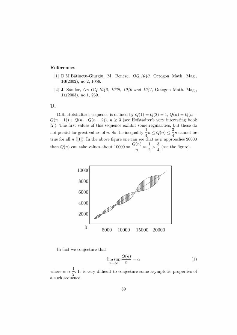
References

[1] D.M.Batinetu-Giurgiu, M. Bencze, OQ.1040, Octogon Math. Mag.,10(2002), no.2, 1056.

[2] J. Sandor, On OQ.1042, 1039, 1040 and 1041, Octogon Math. Mag.,11(2003), no.1, 259.

U.

D.R. Hofstadter’s sequence is defined by Q(1) = Q(2) = 1, Q(n) = Q(n−Q(n − 1)) + Q(n − Q(n − 2)), n ≥ 3 (see Hofstadter’s very interesting book[2]). The first values of this sequence exhibit some regularities, but these do

not persist for great values of n. So the inequality1

4n ≤ Q(n) ≤ 3

4n cannot be

true for all n ([1]). In the above figure one can see that as n approaches 20000

than Q(n) can take values about 10000 soQ(n)

n≈ 1

2>

3

4(see the figure).

0

2000

4000

6000

8000

10000

5000 10000 15000 20000

In fact we conjecture that

lim supn→∞

Q(n)

n= α (1)

where α ≈ 1

2. It is very difficult to conjecture some asymptotic properties of

a such sequence.

89

References

[1] M. Bencze, OQ.525, Octogon Math. Mag., 8(2000), no.2.

[2] D.R. Hofstadter, Godel, Escher, Bach, New York, 1980, 137.

[3] J.H. Conway, Some crazy sequences, Videotaped talk at AT and T BellLabs.

[4] J. Sandor, On the Open Problem OQ.525, Octogon Math. Mag., 9(2001),no.1, 567-568.

3 Determination of certain sequences

A.

We will determine all sequences (xn) such that xn → +∞ and n(xn+1 −xn) → 1 (n → ∞). The sequences of general terms xn = lnn and xn =

1 +1

2+ · · · + 1

nare solutions. This was an OQ of [1]. Since n(xn+1 − xn) → 1

can be written equivalently as

xn+1 − xn

1

n

→ 1, (1)

from Stolz-Cesaro’s theorem it follows that

xn

1 +1

2+ · · · + 1

n

→ 1 (n→ ∞). (2)

Indeed, inan+1 − an

bn+1 − bntake

an = xn, bn = 1 +1

2+ · · · + 1

n→ ∞ (n→ ∞),

soan+1 − an

bn+1 − bn=xn+1 − xn

1

n+ 1

= n(xn+1 − xn)n+ 1

n→ 1.

Thusan

bn→ 1, implying (2).

90

In other words, for any sequence (xn) satisfying (1), relation (2) holds true.Thus

xn ∼ 1 +1

2+ · · · + 1

n= γ + lnn+

1

2n+ α1

1

n2+ α2

1

n4+ . . .

(αi constant), by the Euler-Maclaurin summation formula. Thus xn should beof the form

xn = an

(1 +

1

2+ · · · + 1

n

), (3)

where

an → 1 (n→ ∞). (4)

Reciprocally, if (xn) is given by (3), we must suppose certain auxiliaryconditions of (an). Writing

n

[an+1

(1 +

1

2+ · · · + 1

n+ 1

)− an

(1 +

1

2+ · · · + 1

n

)]

= n

(1 +

1

2+ · · · + 1

n

)(an+1 − an) +

n

n+ 1an+1

sincen

n+ 1an+1 → 1, clearly we must suppose that:

n

(1 +

1

2+ · · · + 1

n

)(an+1 − an) → 0 as n→ ∞. (5)

Therefore, if (4) and (5) are valid, then (1) follows for the sequence (xn)given by (3).

References


[2] J. Sandor, On OQ.813, Octogon Math. Mag., 11(2003), no.1, 226-227.

B.

Determine all sequences (xn) with xn → ∞ and n(xn+1 − xn) → 0 asn→ ∞. An example is given by

xn =n∑

k=2

1

k ln k.

91

Remark that n(xn+1 − xn) → 0 can be writtem asxn+1 − xn

1

n

→ 0, so by

Stolz-Cesaro’s theorem it followsxn

1 +1

2+ · · · + 1

n

→ 0. Indeed, by putting

an = xn, bn = 1 +1

2+ · · · + 1

n,

one has

an+1 − an

bn+1 − bn=xn+1 − xn

1

n+ 1

= n(xn+1 − xn)n+ 1

n→ 0 · 1 = 0,

by assumption, and bn ր ∞, soan

bn→ 0. Thus

xn = an

(1 +

1

2+ · · · + 1

n

),

where an → 0. Reciprocally, if such a sequence satisfies n(xn+1 − xn) → 0,then

n(xn+1 − xn) = n

(1 +

1

2+ · · · + 1

n

)(an+1 − an) +

n

n+ 1an → 0 ⇔

n(xn+1 − xn) = n

(1 +

1

2+ · · · + 1

n

)(an+1 − an) → 0 (n→ ∞).

If one assume xn → ∞, then even the condition an((an+1 − an)) → ∞(n→ ∞) must be supposed.

References



4 A sequence connected with the Wallis product

Let xn given by4n

√

π

(n+

1

4+ xn

) = Cn2n.

92

We will prove that (xn) is convergent, and will find the asymptotical de-velopment of (xn).

Let

Wn =22 · 42 · 62 . . . (2n)2

32 · 52 · 72 . . . (2n − 1)2(2n + 1)

be the general term of the well-known Wallis sequence. Put

Ωn =(2n− 1)!!

(2n)!!.

Then

Wn =1

Ω2n

· 1

2n+ 1(1)

andCn

2n = 4nΩn (2)

which follows immediately. Thus

Cn2n

4n= Ωn.

Now, the asymptotic development of (Ωn) has been given in [2] as follows:

Ωn =1√πn

(1 − 1

8n+

1

128n2+

5

1024n3+ . . .

)(3)

while that of Wn is

Wn =π

2

(1 − 1

4n+

5

32n2− 11

128n3+ . . .

). (4)

By using (1), after a simple calculation it follows (for such calculations,see e.g. [3])

Ω2n =

1

π

(n+

1

4+

1

32− 1

128n2− 5

2048n3+ . . .

) (5)

so, for the sequence (xn) we can write

xn =1

32n− 1

128n2− 5

2048n3+ . . . (6)

This clearly implies also xn → 0 as n→ ∞.Remark. The asymptotic development (3) however appeared earlier in

many places, e.g. Tricomi and Erdelyi (Pacific J. Math. 1(1951), p.133-142).

93

References


[2] L. Toth, A. Vernescu, The asymptotic development of the Wallis se-quence (Romanian), Gaz. Mat. (A), 1/1990, 26-29.

[3] A. Erdelyi, Asymptotic expansions, New York, 1986.

5 A generalized ratio test for series of positiveterms

The main result is contained in the following

Theorem 1. ([2]) Let∞∑

n=1

an be a series with positive terms. Suppose that

there exist a convergent series∞∑

n=1

bn, and a sequence (cn)n≥1 satisfying:

(i) 0 < cn < 1 (n ≥ 1);(ii) cn+m ≤ cncm (n,m ≥ 1),

such thatcnan+1 ≤ cn+1(an + bn) (n ≥ 1). (∗)

Then the series

∞∑

n=1

bn is convergent.

Proof. (i) and (∗) imply

an+1

cn+1≤ an

cn+

bnc+ n

(n ≥ 1). (1)

If we successively take in (1) n = 1, 2, . . . ,m − 1, after addition of thesem− 1 inequalities we get

am

cm≤ a1

c1+b1c1

+ · · · + bm−1

cm−1. (2)

Since cm ≤ cicm−i (by condition (ii)) for all i = 1, 2, . . . ,m − 1 (m ≥ 2),we get from (2) that

am ≤ a1cm−1 + b1cm−1 + b2cm−2 + · · · + bm−1c1 (m ≥ 2). (3)

Now first remark that, since by (ii), cm−1 ≤ cm−11 , and 0 < c1 < 1, so

the series∞∑

m=2

cm−1 is convergent. Since, by assumption, the series∞∑

m=2

bm−1 is

94

also convergent, by a well-known theorem by Mertens (see e.g. [3]), the seriesof general term b1cm−1 + b2cm−2 + · · ·+ bn−1c1 will be convergent, too. Thus,inequality (3) finishes the proof of the theorem.

Corollary. A series of decreasing positive terms∞∑

n=1

an is convergent if

and only if there exists a convergent series of nonnegative terms

∞∑

n=1

bn, and a

sequence (cn) satisfying (i) and (ii) such that (∗) holds true.Proof. The sufficiency follows by the theorem. For the necessity part, take

bn = kan (n ≥ 1, k > 0), cn =1

(1 + k)n(n ≥ 1). Then (i), (ii) hold true, while

(∗) becomes an+1 ≤ an, which is also true, by assumption.Remark. By letting cn = kn (0 < k < 1), from Theorem 1 we get the

following result by V. Berinde [1]:Theorem 2. Let an > 0 (n ≥ 1). If there exists a convergent series of

nonnegative terms

∞∑

n=1

bn such that

an+1

an + bn≤ k < 1 for n ≥ 1, (4)

then

∞∑

n=1

an is convergent.

References

[1] V. Berinde, Une generalisation de critere de d’Alembert pour les seriespositives, Bul. St. Univ. Baia Mare, 7(1991), 21-26.

[2] V. Berinde, J. Sandor, On the generalized ratio test, Bul. St. Univ. BaiaMare, 11(1995), 55-58.

[3] T.J.I’A. Bromwich, An introduction to the theory of infinite series, Thirded., 1991 by Chelsea AMS Publishing.

6 A generalization of Bereznai’s theorem on infiniteseries

The following theorem is due to the Hungarian mathematician GyulaBereznai (1921-1990):

95

Let (an) be a sequence of positive numbers, such that there exists p ∈ R

with

(an

an+1

)n

≥ p > e (n = 1, 2, . . . ). Then the series∞∑

n=1

an is convergent. If

(an

an+1

)n

≤ e, then the series is divergent. The following generalization will

be proved:Theorem. Let us suppose that there exist a sequence (λn) of positive num-

bers and a real number p such that(

an

an+1λn

)n

≥ p > e. (1)

Put q = ln p. If the series

∞∑

n=1

λ1λ2 . . . λn

nqis convergent then the se-

ries

∞∑

n=1

an will be convergent, too. If

(an

an+1λn

)n

≤ e, and the series

∞∑

n=1

λ1λ2 . . . λn

nis divergent, then the series

∞∑

n=1

an will be divergent, too.

Proof. By taking logarithms in (1) one gets

n(log an − log an+1 + log λn) ≥ log p = q > 1.

By writing this inequality for n = 1, 2, 3, . . . , n; after addition one gets

log a1 − log a2 + log2 − loga + · · · + log an−1 − log an + log an − log an+1

+ log(λ1λ2 . . . λn) ≥ q

(1 +

1

2+ · · · + 1

n

),

so

log an+1 ≤ log a1 + log(λ1 . . . λn) − q

(1 +

1

2+ · · · + 1

n

),

i.e.an+1 ≤ a1(λ1 . . . λn)e−q(1+ 1

2+···+ 1

n). (2)

Now, for the Euler sequence (γn), given by

γn = 1 +1

2+ · · · + 1

n− log n,

it is well known that 0 < γn < 1, so

log n < 1 +1

2+ · · · + 1

n< log n+ 1 (3)

96

implying

e−q(1+···+ 1n) <

1

nq. (4)

Now, (2), (4) give

an+1 < a1λ1 . . . λn

nq,

so if the series

∞∑

n=1

λ1 . . . λn

nqis convergent, clearly, by the comparison theorem

of series of positive terms, the series∞∑

n=1

an will be convergent, too. This finishes

the proof of the first part of the theorem.The proof of the second part runs in the same lines. Indeed, from

n(log an − log an+1 + log λn) ≤ 1 (5)

after summation one obtains

log a1 − log an+1 + log(λ1 . . . λn) ≤ 1 +1

2+ · · · + 1

n,

soan+1 ≥ a1

e1+12+···+ 1

n

(λ1 . . . λn). (6)

Now, by the right side of (3) e1+12+···+ 1

n < en, so by (6) one has

an+1 >a1

e· λ1 . . . λn

n(7)

and the divergence of the series

∞∑

n=1

λ1 . . . λn

nwill imply at once that of the

series

∞∑

n=1

an.

Remark 1. For λn ≡ 1 the Bereznai theorem is reobtained.Remark 2. We have assumed (1) etc. to hold for all n ≥ 1. It is not difficult

to see that it would be sufficient to assume these inequalities for sufficientlylarge n, i.e. n ≥ n0.

References

[1] L. Filep, In memorian Bereznai Gyula, particular letter, dated 7th De-cember 2002, Containing a xerox copy of an obituary of Gy. Bereznai’slife and work.

97

[2] J. Sandor, A generalization of Bereznai’s theorem, Octogon Math. Mag.,11(2003), no.2, 480-481.

7 The iteration of sin and cos and two infinite series

Let un+1 = sinun, vn+1 = cos vn (n ≥ 0), where u0, v0 are given realnumbers. We will consider the following sums:

1)

∞∑

n=1

un

n; 2)

∞∑

n=1

vn

n.

While the sum 1) puts problems, since this series is indeed convergent,the second sum 2) will be divergent. This last assertion follows from the factthat the sequence (vn) is convergent to a positive number a > 0. Then clearly

vn >a

2for n ≥ n0, therefore

∑

n≥n0

vn

n>a

2

∑

n≥n0

1

n,

and the harmonic sum is divergent. We will prove that a is the single root ofthe equation x = cos x, x ∈ (0, 1). We have:

|vk+1 − a| = | cos vk − cos a| = 2

∣∣∣∣sinvk + a

2sin

vk − a

2

∣∣∣∣ ,

wherevk + a

2∈ [0, 1] ⊂

(0,π

2

), and

|vk − a|2

∈ [0, 1) ⊂(0,π

2

), for k ≥ 2.

(Here v1 = cos v0 ∈ [−1, 1], but v2 = cos v1 ∈ (0, 1), so by induction vk ∈ (0, 1),

for all k ≥ 2). Thus, for k ≥ 2 one has sinvk + a

2< sin 1,

∣∣∣∣sina− vk

2

∣∣∣∣ ≤|vk − a|

2, which yields |vk+1 − a| < (sin 1)|vk − a| (k ≥ 2) implying |vk − a| <

(sin 1)k−2|v2 − a|, vk → a (k → ∞), since 0 < sin 1 < 1.

The first sum is convergent, since it is known ([2]) that un ≤ 2√n+ 1

,

which follows e.g. from the inequality sinx ≤ x− x3

6+

x5

120for x ∈

[0,π

2

](it

is sufficient to consider such x) so

un+1 = sinun ≤ sin2√n+ 1

≤ 2√n+ 1

− 1

6

(2√n+ 1

)3

+1

120

(2√n+ 1

)5

≤ 2√n+ 1

98

and by induction this inequality follows.

On the other hand, the inequality sinx ≥ x

x+ 1(x ∈ (0, 1)) implies by

induction un ≥ x

x+ n. This implies also that the series

∞∑

n=1

un is divergent.

The series

∞∑

n=1

un

nis convergent, since

un

n≤ 2

n√n+ 2

<2

n√n

=2

n3/2,

and the series∞∑

n=1

1

nαis known to be convergent for α > 1.

It is well known that un ∼√

3

nas n→ ∞ ([1]), and in fact un <

√3

n, for

all n ≥ 1. Therefore

∞∑

n=1

un

n<

√3 · ζ

(3

2

), where ζ(α) =

∞∑

n=1

1

nα(α > 1) is the

Riemann zeta-function.

References

[1] N.G. De Bruijn, Asymptotic methods in analysis, Amsterdam, 1961.

[2] F. Bencherif, G. Robin, Sur l’itere de sinx, Publ. l’Inst. Math., 56(70),1994, 41-53.

8 On Olivier’s criterion

1. Let

∞∑

n=1

an be an infinite series with positive terms. Put

sn = a1 + a2 + · · · + an.

Since sn+1 − sn = an+1 if sn → s ∈ R (n → ∞) (i.e., the series is con-vergent), we get an+1 → 0, i.e. an → 0 as n → ∞. The following importantcriterion is due to L. Olivier (see e.g. K. Knopp [4]).

Theorem. If the series

∞∑

n=1

an with the positive terms and decreasing gen-

eral term (an) is convergent, then

nan → 0 as n→ ∞. (1)

99

The following proof is simpler than the usually known ones (see e.g. [2]).Remark that

na2n ≤ an+1 + an+2 + · · · + a2n = s2n − sn → s− s = 0 as n→ ∞.

This implies na2n → 0, so

2na2n → 0 as n→ ∞. (∗)

In a similar way,

(n+ 1)a2n+1 ≤ an+1 + · · · + a2n+1 = s2n+1 − sn → s− s = 0

so (n + 1)a2n+1 → 0. This implies (2n + 2)a2n+1 → 0, so (2n + 1)a2n+1 =(2n+ 2)a2n+1 − a2n+1 → 0, as a2n+1 → 0, n→ ∞. Thus

(2n + 1)a2n+1 → 0 (∗∗)

Clearly, (∗) and (∗∗) give mam → 0 as m→ ∞, proving (1).2. In three recent Open Question ([1-4]) Amarnath Murthy posed the

problem of summation of series:

1)∞∑

n=1

(212n − 1); 2)

∞∑

n=1

(k12n − 1); 3)

∞∑

n=1

(k1

kn − 1).

These three series in fact all are divergent. Put an = 212n −1. Then an → 0

as n → ∞, an+1 − an = 21

2(n+1) − 212n < 0 as 2

n+1n = 21+ 1

n > 2. On the otherhand,

nan =2

12n − 1

1

n

→ ln 212 = ln

√2 6= 0 as n→ ∞.

By Olivier’s criterion, the series cannot be convergent.

For the case 2) nan → 1

2ln k, while in case 3) nan → 1

kln k as n → ∞.

Since ln k 6= 0 (k 6= 1), all series are divergent.

References

[1] Amarnath Murthy, OQ.927, OQ.928, OQ.929, Octogon Math. Mag.,10(2002), no.1, 533, 534.

[2] K. Knopp, Theorie und anwendung der unendlichen Reichen, (FunfteAuflage), 1964, Springer Verlag, 125-126.

100

9 On Dirichlet’s beta function

The OQ.546 proposed by M. Bencze is a very interesting problem. Let

Sk = 1 − 1

3k+

1

5k− 1

7k+ · · · =

∞∑

n=0

(−1)n

(2n + 1)k, k ∈ N∗.

Since 0 < Sk < 1 for all k, clearly [Sk] = 0. For negative k, Sk is diver-gent. On the other hand, the irrationality of Sk is known only for odd k. Ageneralization of Sk is Dirichlet’s beta function

β(x) =∞∑

n=0

(−1)n

(2n+ 1)x, x ≥ 1

(see [2]). Let (En) be the sequence of Euler numbers, i.e. given by the relation

2ex

e2x + 1=

∞∑

k=0

Ekxk

k.

It can be shown that all Euler numbers are integers, E0 = 1, E2 = −1,E4 = 5, E6 = −61, . . . and E2n−1 = 0, for all n ≥ 1. (Unfortunately, sometimesan alternate definition of the Euler numbers appears, in this definition thesubscripts are sometimes different and all numbers are positive). Now, it iswell-known that ([2])

β(2m+ 1) =(−1)mE2m

2 · (2m)!

(π2

)2m+1(m ≥ 0)

(e.g. β(1) =π

4, β(3) =

π3

32, β(5) =

5π5

1536). Therefore S2m+1 are all irrational,

and even transcendental. (Since π2m+1 is known to be transcendental). On theother hand, the values of Sk for k even (i.e. β(2m)) are not known. It is known([2]) that for all x one has

β(x) =∏

p≡1 (mod 4)

(1 − 1

px

)−1 ∏

p≡3 (mod 4)

(1 +

1

px

)−1

(where p denotes a prime). For k = 2, S2 is known as Catalan’s constant,denoted by G. We have G ≈ 0.91596 . . . , but it is not known, if G is irrational([3], [4]). We note here that G has applications in statistical mechanics (e.g.dinner problem [5]). For many related questions, see also Chapter 5 of [6].

101

References


[2] G.H. Hardy, E.M. Wright, An introduction to the theory of numbers,Oxford, 1979.

[3] J. Choi, The Cataln’s constanr and series involving the Zeta functions,Comm. Korean Math. Soc., 13(1998).

[4] D. Bradley, A class of series acceleration formulae for Catalan’s constant,The Ramanujan Journal, 3(1999), 159-173.

[5] D.A. Lavis, G.M. Bell, Statistical mechanics of lattice systems, SpringerVerlag, 1999.

[6] J. Sandor, Handbook of number theory II, Springer Verlag, 2004.

10 On sequences related to the sum of powers ofpositive integers

1. Let Sp(n) =

n∑

j=1

jp (p > 0) be the sum of pth powers of the first n

positive integers. Put Gp(n) = Sp(n)np+1 (n ≥ 1).Recently, S.S. Dragomir and J. can der Hoek [4] proved the following re-

sults:(i) For p ≥ 1 one has

Gp(n) ≥ (n+ 1)p/[(n+ 1)p+1 − np+1].

(ii) For p ≥ 1,

Gp(n+ 1) ≤ Gp(n) (n ≥ 1).

(iii) Let 0 ≤ aj ≤ 1 (j = 1, n). Then

n∑

j=1

jpaj ≥ Gp(n)

n∑

j=1

aj

p+1

for p ≥ 1 (p ∈ R).

In fact, (ii) is equivalent with (i), as can be seen by elementary transfor-mations, while (iii) can be deduce from (i), as well. In the above mentionedpaper, the authors obtain interesting applications of (iii) in guessing theory.

102

2. Inequality (i) is exactly inequality (2) from [9] (with r in place of p),where it is proved that this relation holds true for all p > 0, and with strictinequality. This is essentially due to H. Alzer [1]. The history of this inequalityis the following: By investigating a problem of Lorentz sequence spaces, in 1988J.S. Martins [7] discovered certain interesting inequalities for Sp(n). Let

Lp(n) = [(n+ 1)Sp(n)/nSp(n+ 1)]1/p (p > 0)

andxn = (n!)1/n/((n + 1)!)1/(n+1), yn = n/(n+ 1) (n ≥ 1).

Martins proved that (for p > 0, n ≥ 1)

Lp(n) ≤ xn (1)

and in 1993, Alzer [1] established the reverse inequality

Lp(n) ≥ yn. (2)

It is not difficult to see that limp→0

Lp(n) = xn, limp→0

Lp(n) = yn (see e.g. [5],

[6]), so the bounds (1) and (2) are best possible. Quite recently the author[9] has obtained a simple method to prove the inequality (2) (by showing firstthat it is equivalent to (i) for p > 0). This proof is based on mathematicalinduction and Cauchy’s mean value theorem of differential calculus. We noticethat in [4] the method is based on convex functions.

In 1992 G. Bennett [3] proved the inequalities

Lp(n) ≤ n+ 1

n+ 2for p ≥ 1 (3)

and

Lp(n) ≥ n+ 1

n+ 2for 0 n+ 1

n+ 2(see e.g. [7] or [8]), and

n+ 1

n+ 2>

n

n+ 1, the inequalities

(3) and (4) are refinements of (1) and (2) for p ≥ 1 and respectively 0 < p ≤ 1.The proof of (3) and (4) given in [3] is quite difficult. In [10] we have obtainedan easy proof, based on mathematical induction and Lagrange’s mean valuetheorem of differential calculus.

3. An analogous expression introduced in [3] is Qp(n) with j−p instead ofjp in the definition of Lp(n). It is proved there that

Qp(n) ≤ n+ 2

n+ 1(r > 0, n ≥ 1). (5)

103

A recent refinement of (5) has been obtained in [2], namely that

Qp(n) ≤ 1

xn. (6)

A new proof of this result, by using the theory of Euler’s gamma function,is due to the author (unpublished). Finally, we note that the inequalities (3)-(5) have noteworthy applications in the theory of the so-called power meansmatrices (see [3]).

References

[1] H. Alzer, On an inequality of H. Minc and I. Sathre, J. Math. Anal.Appl., 179(1993), 396-402.

[2] H. Alzer, Refinement of an inequality of G. Bennett, Discrete Math.,135(1994), 39-46.

[3] G. Bennett, Lower bounds for matrices, II, Canad. J. Math., 44(1992),54-74.

[4] S.S. Dragomir, J. van der Hoek, Some new analytic inequalities and theirapplications in guessing theory, J. Math. Anal. Appl., 225(1998), 542-556.

[5] G.H. Hardy, J.E. Littlewood, G. Polya, Inequalities, Cambridge Univ.Press, Cambridge, 1952.


[7] J.S. Martins, Arithmetic and geometric means, an application to Lorentzsequence spaces, Math. Nachr., 139(1988), 281-288.

[8] J. Sandor, Sur la fonction Gamma, Centre Rech Math. Pures, Neuchatel,Serie I, Fasc. 21(1989), 4-7.

[9] J. Sandor, On an inequality of Alzer, J. Math. Anal. Appl., 192(1995),1034-1035.

[10] J. Sandor, On an inequality of Bennett, General Mathematics, Sibiu,3(1995), no.3-4, 121-125.

104

Chapter 3

Special numbers andsequences of integers

”... Therefore, if we crave for the goal that is worthy and fitting for man,namely, happiness of life... arithmetic... which is the mother of geometry...”

(Nicomachus of Gerasa)

”... Mathematicians have tried in vain to this day to discover some orderin the sequence of prime numbers, and we have reason to believe that it is amystery into which the human mind will never penetrate.”

(Leonhard Euler)

105

1 On pn/ lnn

Let the sequence (xn) defined by: xn :=pn

lnn, where pn is the nth prime

number. Holds true the followingTheorem. For n ≥ 2, there holds xn < xn+1.Proof. A direct check shows x2 < x3 < · · · < x20. We let further on be

n ≥ 20. The claimed inequality xn < xn+1 is in equivalent form

pn <lnn

ln(n+ 1)pn+1. (∗)

Because of pn1 ≥ pn +2 it is for (∗) enough to prove the sharper inequality

pn <lnn

ln(n+ 1)(pn + 2),

i.e.

pn <2 lnn

ln

(1 +

1

n

) . (∗∗)

We now take from [1], p.247 the sharp upper bound for pn proved by Rosserand Schoenfeld, i.e.

pn < n

(lnn+ ln lnn− 1

2

),

whenever n ≥ 20. Using the familiar relations ln

(1 +

1

n

)<

1

nand lnn < n

we thus get

pn < n

(lnn+ ln lnn− 1

2

)< 2n lnn <

2 lnn

ln

(1 +

1

n

) ,

i.e. (∗∗).This proof is due to W. Janous [2].

References

[1] J. Sandor, D.S. Mitrinovic, B. Crstici, Handbook of number theory,Kluwer, Dordrecht, 1996, and Springer Verlag, 2005.

[2] W. Janous, A solution of the Open Question OQ.663, Octogon Math.Mag., 9(2001), no.2, 958.

106

2 On the integer part of n

√pk

Let pk denote the kth prime number. In OQ.608, in [1] it is conjecturedthat ([ n

√pk])k∈N is a sequence which contains infinitely many primes (n ≥ 2

given). In fact, much stronger results are known. If 0 < c <5

6is a fixed

constant, then for the number πc(x) of primes p ≤ x for which [pc] is prime, is

∼ 1

cx/ log2 x, x → ∞. This result is due to A. Balog [2]. Let c =

1

n≤ 1

2<

5

6for n ≥ 2. Put x = pk. Then the number of primes which occur between

[ n√p1], [ n

√p2], . . . , [ n

√pk] is ∼ npk

log2 pk

∼ nk log k

log2 k= n

k

log2 k. For fixed n and

k → ∞, we have nk/ log2 k → ∞. See also [4] (e.g. p.301) for primes inspecial sequences. For exact formulae involving [ n

√pk] we note that recently,

by improving earlier results by Rosser and Schonfeld, P. Dusart [3] proved thatfor k ≥ k0 (= computable constant)

k

(log k + log log k − 1 +

log log k − α0

log k

)≤ pk

≤ k

(log k + log log k − 1 +

log log k − α1

log k

),

where a0 = 2, 25; α1 = 1, 8.For example, for n = 2 one can deduce that [

√pk] is one of

[√k(log k + log log k − 1)] or [

√k(log k + log log k − 1)] + 1.

References


[2] A. Balog, On a variant of the Pjateckii-Sapiro prime number theorem,Groupe de travail en Th. Anal. et Elem. Nomb. 1987-1988, 3-11. Publ.Math. Orsay, 89-01, Univ. Paris XI, Orsay 1989.

[3] P. Dusart, The kth prime is greater than k(ln k + ln ln k − 1) for k ≥ 2,Math. Comp. 68(1999), no.225, 411-415.

[4] J. Sandor, D.S. Mitrinovic, (in coop. with B. Crstici), Handbook of num-ber theory, Kluwer Acad. Publ. 1995, and Springer Verlag, 2005.

107

3 [ex] and [ey] as consecutive primes

We will prove that [ex] and [ey] cannot be consecutive prime numbers forany x 6= y positive integers. It is sufficient to consider y > x. Then y ≥ x+ 1,and [ey] ≥ [ex+1]. We will prove that

[ex+1] − [ex] > 2, for any x ≥ 1. (1)

Indeed, by [a] > a− 1 and [a] ≤ a we have:

[ex+1] − [ex] > ex+1 − ex − 1 = ex(e− 1) − 1 ≥ e(e − 1) − 1

≈ 4, 6 − 1 = 3, 6 > 2,

which proves (1). Thus [ex] and [ey] cannot be consecutive prime numbers.Remark. Clearly [ex] can be prime, e.g. [e1] = 2, [e2] = 7, etc. An inter-

esting problem would be the study of the proportion of primes in the sequence[e1], [e2], . . . , [en], n > 1. The same result (with same proof) holds true, whene is replaced with the number π.

4 On a sequence connected with the number ofprimes

Let π(x) denote the number of primes ≤ x, and let (xn) be a sequencedefined by

π(n) =n

log n

(1 +

xn

log n

). (1)

We will study the convergence and the asymptotical development of (xn).We note here that this follows essentially from the prime-number theorem inthe form proved by the la Vallee-Poussin [1]

π(x) =

∫ x

2

dt

log t+R(x), x→ ∞ (2)

where R(x) = O(x exp(−A√

log x)) (A > 0 constant).Now, by partial integration

∫ x

2

dt

log t=

x

log x+

∫ x

2

1

log2 tdt+ c1

∫ x

2

1

log2 tdt =

x

log2 x+ 2

∫ x

2

1dt

log3 t+ c2

108

∫ x

2

1

log3 tdt =

x

log3 x+ 3

∫ x

2

1

log4 tdt+ c3,

and by induction it follows

∫ x

2

dt

log t=

x

log x+

x

log2 x+

2x

log3 x+

6x

log4 x

+24x

log5 x+ · · · + (k − 1)!x

logk x+ k!

∫ x

2

1

logk+1 tdt+ c

(c a constant). Therefore

xn = 1 +2

log n+

6

log3 n+

24

log4 n+ · · · + (k − 1)!

logk n+O

(1

logk+1 n

)

giving xn → 1 (n→ ∞) and the asymptotical development of xn.Remark. Improvements of (2) have been obtained by J.E. Littlewood,

H.M. Korobov, I.M. Vinogradov, etc., see [2].

References

[1] C.J. de la Vallee-Poussin, Sur la fonction ζ(s) de Riemann et le nombredes nombres premiers inferieures a une limite donnee, Mem. Couronneset autres mem. Publ. l’Acad. Roy. Sci. Lettres Beaux-Arts Belgique,59(1899-1900), no.1, 74.

[2] J. Sandor, D.S. Mitrinovic, Handbook of number theory, Kluwer Acad.Publ., 1996, and Springer Verlag, 2005.

5 The smallest number of ones

Let F (n) denote the smallest number of ones that can be used to representa positive integer n using ones and any number of the symbols +, ·, ( ). InOQ.612 in [1], there are stated certain conjectures on F (n). One of themstates that there exists at least a prime between F (n) and F (n + 2). We willprove that this is true. It is known (see e.g. [2]) that

3 log3 n ≤ F (n) ≤ 5 log3 n (1)

where the logarithms are taken in base 3. Therefore

F (n+ 2) ≤ 5 log3(n+ 2).

109

We will show that in fact one can take F (n+ 1). Indeed, by a result of J.

Nagura [3], for x ≥ 25 there is at least a prime between x and6

5x. Now, let

x = 3 log3 n. Then6

5(3 log3 n) < 5 log3(n+ 1)

sincelog3(n+ 1)

log3 n> 1 >

18

25.

Since

F (n+ 1) ≤ 5 log3(n+ 1),

there is a prime between F (n) and F (n + 1), if x = 3 log3 n ≥ 25, i.e. n ≥3

253 ≈ 383. This is true for n ≥ 39 = 19683. For smaller values of n, a computer

search can be done.

References


[2] R.K. Guy, Some suspiciously simple sequences, Amer. Math. Monthly,93(1986), 186-190; 94(1987), 965; 96(1989), 905.

[3] J. Nagura, On the interval containing at least one prime number, Proc.Japan Acad., 28(1952), 177-181.

6 On the sequence of composite numbers

Let (cn) denote the sequence of composite numbers. Based on an idea byP. Vlamos [3], we will prove the following:

Theorem. The sequence (un) of general term un = cn/ log n is strictlyincreasing for n ≥ 2.

The proof is based on the followingLemma. For n ≥ 8 one has cn < n log n.Proof. Since cn = π(cn)+n+1, where π(x) denotes the number of primes

≤ x, by the known inequality (see e.g. [1], [2])

π(x) ≤ x/(log x− 3/2) for x ≥ 5,

we get for n ≥ 2 that

cnlog cn − 5/2

log cn − 3/2< n+ 1. (1)

110

Let us consider the function

f(x) = xlog x− 5/2

log x− 3/2.

It is easy to verify that this function is increasing for x ≥ 5. Thus, ifcn ≥ n log n, then (1) would imply

n+ 1 ≥ n log nlog n+ log log n− 5/2

log n+ log log n− 3/2. (2)

For n ≥ 10, by n log n ≥ 2(n+ 1), (2) implies trivially that

1 ≥ 2log n+ log log n− 5/2

log n+ log log n− 3/2,

false for n ≥ 13. Thus, the Lemma is true for n ≥ 13. For 8 ≤ n ≤ 12, a directverification applies.

The proof of Theorem follows easily by the Lemma, since

un+1 − un ≥ cn + 1

n log(n+ 1)− cnn log n

=1

log(n+ 1)

1 −cn log

(1 +

1

n

)n

n log n

≥ 1

log(n + 1)

[1 − cn

n log n

]> 0

for n ≥ 8. For 2 ≤ n ≤ 7, a direct verification completes the proof.

References

[1] J.B. Rosser, L. Schoenfeld, Approximate formulas for some functions ofprime numbers, Illinois J. Math., 6(1962), 64-92.

[2] J. Sandor, D.S. Mitrinovic, Handbook of number theory, Kluwer Acad.Publ., 1996.

[3] P. Vlamos, On the monotony of certain sequences, Octogon Math. Mag.,10(2002), no.1, 370-371.

111

7 A note on Bernoulli numbers

Let

ζ(s) =∞∑

n=1

1

ns, s > 1

be the Riemann Zeta function. Then it is well-known that

|B2n| =2(2n)!ζ(2n)

(2π)2n

(see e.g. [2]). Therefore, after an easy calculation we have:

∣∣∣∣B4nB4n−2

B42n

∣∣∣∣ =(2n)!(4n − 2)!

[(2n)!]4A(n),

where

A(n) =π2ζ(4n)ζ(4n− 2)

[ζ(2n)]4.

Since by Euler’s formula

ζ(s) =∏

p prime

(1 − p−s)−1,

it is immediate that limn→∞

A(n) = π2. Put

xn =(4n)!(4n − 2)!

[(2n)!]4.

By the well-known Stirling formula one has

n! ∼√

2πnnne−n

(see [2] for an elementary proof of an improved version), we get

xn ∼√

2π(4n)(4n)4ne−4n√

2π(4n − 2)(4n− 2)4n−2·

·e−(4n−2)/(√

2π · 2n)2(2n)8ne−8n.

Since

(4n − 2)4n−2

n4n−2=

(4 − 2

n

)4n−2

= 44n−2

[(1 − 1

2n

)−2n] 4n−2

−2n

∼ 44n−2e−2,

112

after certain computations we get xn ∼ 44n

n3

1

32π(n→ ∞).

By extending the definition of A(n) to

A(s) =π2ζ(4s)ζ(4s− 2)

[ζ(2s)]4,

by logarithmic differentiation we can deduce

A′(s)A(s)

=−8ζ ′(2s)ζ(2s)

+4ζ ′(4s)ζ(4s)

+4ζ ′(4s− 2)

ζ(4s− 2)

=

∞∑

n=1

Λ(n)

(8

n2s− 4

n4s− 4

n4s−2

)> 0

for s > 1 (where Λ is the von Mangoldt function, see [1]) we have A′(s) > 0,∀ s > 1, i.e. A is strictly increasing in this domain. Therefore A(n) < π2,implying ∣∣∣∣

B4n ·B4n−2

B42n

∣∣∣∣ < π2xn.

References

[1] T.M. Apostol, Introduction to analytic number theory, Springer Verlag,1976.

[2] J. Sandor, On Stirling’s formula (Romanian), Lucr. Semin. Did. Mat.,14(1998), 235-239.

8 The number of factorizations of n

Let f(n) be the number of ”essentially different factorizations” of n, i.e.the number of representations of the positive integer n as a product of integralfactors larger than 1, a change in the order of factors not counting as a distinctrepresentation. In OQ.528, proposed by M. Bencze it is conjectured that

f(n) ≤ n− 1

n!for n ≥ 10.

In fact, much stronger relations are known in the literature. W. Chen [2]proved that

f(n) ≤ n

4+ 1 for all n.

113

Clearlyn

4+ 1 < n− 1

n!⇔ 3n

4> 1 +

1

n!.

This is true for all n ≥ 3. (Indeed,1

n!≤ 1

2n≤ 1

2nfor n ≥ 4, while

3n

4> 1 +

1

2n=

2n+ 1

2nsince 3n2 > 4n + 2. For n = 3, a direct verification is

valid). F.W. Dodd and L.E. Matties [3] proved that

f(n) ≤ n

(log n)α

for all fixed α > 0 and n sufficiently large; if the least prime factor of n is> 3, then f(n) < n/ log n, proved by H.Z. Cao [4]. It is conjectured that

f(n) ≤ n

log nfor n 6= 144, but this is open, as far as know. For other results,

see [5].

References


[2] W. Chen, Upper bound if the number of multiplicative partitions (Chi-nese), Acta Math. Sinica, 32(1989), 604-609.

[3] F.W. Dodd, L.E. Matties, Estimating the number of multiplicative par-titions, Rocky Mountain J. Math., 17(1987), 797-813.

[4] H.Z. Cao, On a conjecture of multiplicative partitions, Rend. Mat. Appl.7, Ser.11, no.4(1991), 729-735.

[5] J. Sandor, D.S. Mitrinovic, Handbook of number theory, Kluwer Acad-emic Publishers, 1996.

9 On perfect and m-perfect numbers

This note is in connection with the paper [1] and the Open Problem OQ.113(Octogon Math. Mag., 5(1997), no.2). First we wish to note that the terminol-ogy of ”very perfect numbers” is not known, but the ”superperfect numbers”one is well-known.

Thus, D. Suryanarayana [7] calls a number n superperfect if σ(σ(n)) = 2nand he and H.J. Kanold [7], [4] obtain the general form of even superperfectnumbers. Kanold [4] proves that all odd superperfect numbers are perfect

114

squares, but we do not know if there exists at least one number of this type. D.Suryanarayana [8] shows that there is no superperfect number of the form p2α,and this is more general than the result by Bencze, Popovici and Smarandache[1].

More generally, D. Bode [2] defines m-perfect numbers as numbers n forwhich

σ(σ . . . σ(n) . . . )︸︷︷︸m

= 2n,

and shows that for m ≥ 3 there are no even m-perfect numbers. The author[5] calls the superperfect numbers as σ σ-numbers. Let ψ(n) be the Dedekindfunction,

ψ(n) = n∏

p/n

(1 +

1

p

), ψ(1) = 1 (p prime).

In our paper [5] many problems related to ψ ψ-perfect numbers andvariants are considered. Among others there it is proved the following (seep.10) inequality:

σ(σ(n)) ≥ ψ(σ(n)) ≥ 2n (1)

for all even n, with equality only for n = 2k, where 2k+1 − 1 = prime. By thisrelation, we can reobtain Suryanarayana’s and Kanold’s result on the form ofeven superperfect numbers. A new proof of this is obtained in [6], too.

But our aim in this note is to prove a part of OQ.113, namely that for allk ≥ 3 there are arbitrarily long sequences of consecutive integers n such that

σ σ · · · σ(n)︸︷︷︸k

> 2n. (2)

First remark, that when σ(n) is even, from (1) we get

σ(σ(σ(n))) ≥ 2σ(n) ≥ 2(n + 1) > 2n

and this can be continued, and thus (2) remains true for all k ≥ 3, when σ(n)is even.

Now, we recall the well known fact (see [3]) that σ(n) is odd only whenn = a2 or n = 2a2 (a ∈ N∗). We will show that there exist arbitrary longsequences with consecutive terms in which no term is of the form a2 or 2a2.

Let Pi (i = 1,m) be m distinct odd primes, where m is given. By theChinese Remainder Theorem there exists x ∈ N with the property

x ≡ Pi − i+ 1 (mod P 2i ), i = 1, 2, . . . ,m. (3)

115

Then x, x+ 1, . . . , x+m− 1 are m consecutive integers and no one can beof the form a2 or 2a2 since, on base of (3),

xi − 1 = P 2i ki + Pi, ki ∈ N

and this is divisible by Pi but not by P 2i (Pi odd prime).

References

[1] M. Bencze, F. Popovici, F. Smarandache, About very perfect numbers,Octogon Math. Mag., 5(1997), no.2, 53-54.

[2] D. Bode, Uber eine Verallgemeinerung der Vollkommen Zahlen, Disser-tation, Braunnschweig, 1971.

[3] G.H. Hardy, E.M. Wright, An introduction to the theory of numbers, 4ed,Oxford Univ. Press, 1960.

[4] H.J. Kanold, Uber ”Superperfect numbers”, Elem. Math. 24(1969), 61-62.

[5] J. Sandor, On the composition of some arithmetic functions, StudiaUniv. Babes-Bolyai, Math., XXXIV, 1, 1989, 7-14.

[6] J. Sandor, On even perfect and superperfect numbers (Romanian), Sem.Did. Mat., 8(1992), 167-168.

[7] D. Suryanarayana, Superperfect numbers, Elem. Math., 14(1969), 16-17.

[8] D. Suryanarayana, There is no superperfect number of the form p2α,Elem. Math., 28(1973), 148-150.

10 On Ruzsa’s lovely pairs

1. In paper [3] we have studied, among others, also the following problemof I.Z. Ruzsa [4]: Find all numbers a, b such that

σ(a) = 2b, σ(b) = 2a. (1)

Ruzsa called these numbers (a, b) a lovely pair (or lovely numbers), and inan unpublished manuscript he showed that if a and b are both even, then

a = 2k(2q+1 − 1), b = 2q(2k+1 − 1) (2)

116

where 2k+1−1 and 2q+1−1 are both primes. Sandor [3] defined a super-lovelypair by

σ(σ(a)) = 2b, σ(σ(b)) = 2a (3)

and proved that if a and b are both even, then a = b, i.e. a and b are super-perfect numbers. (He also gave a new proof of (2)). Since in a recent O.Q. [6] ageneralization of (1) to more numbers (and with p in place of 2) is considered,we shall present here our elementary method on the above stated results.

2. Let a = 2kA, b = 2ab, where k, q ≥ 1 and A,B are odd numbers. Sinceσ is a multiplicative function σ(a) = (2k+1 − 1)σ(A), etc., so one has

(2k+1 − 1)σ(A) = 2q+1B, (2q+1 − 1)σ(B) = 2k+1A.

Since 2k+1 − 1 divides 2q+1B, and is odd, B is divisible by 2k+1 − 1, i.e.B = (2k+1 − 1)B′; similarly A = (2q+1 − 1)A′ with A′, B′ odd numbers. Onegets

σ(A) = 2q+1B′, σ(B) = 2k+1A′. (4)

Now, using the inequality σ(mn) ≥ mσ(n) with equality only for m = 1(see e.g. [1], [2]), one can write 2q+1B ≥ (2k+1−1)A′ ·2q+1 (where we have usedalso σ(m) ≥ m + 1 with equality only for m = prime), so we have B′ ≥ A′.The inequality B′ ≥ A′ follows in the same manner. Thus A′ = B′, and (4)gives A = (2k+1 − 1)S, B = (2q+1 − 1)S with 2k+1 − 1 and 2q+1 − 1 bothprimes. Since σ(B) = 2k+1S, σ(A) = 2q+1S and σ((2q+1 − 1)S) ≥ S · 2q+1

with equalities, only if S = 1 and 2q+1 − 1 = prime, we get B = 2k+1 − 1,A = 2q+1 − 1. So (2) is proved.

3. Now let a = 2kA, b = 2qB be a solution of (3) with a, b both even. Thenσ(a) = (2k+1 − 1)σ(A), σ(b) = (2q+1 − 1)σ(B) and (3) becomes

σ((2k+1 − 1)σ(A)) = 2q+1B, σ((2q+1 − 1)σ(B)) = 2k+1A. (5)

By the above method, one can write successively

2q+1B ≥ σ(A)2k+1 ≥ A · 2k+1, 2k+1A ≥ σ(B) · 2q+1 ≥ B · 2q+1,

so2q+1B ≥ σ(A)2k+1 ≥ A · 2k+1 ≥ σ(B) · 2q+1 ≥ B · 2q+1. (6)

By (6) we must have equalities in all signs of inequalities, implying A =B = 1 and 2k+1 − 1 = prime, 2q+1 − 1 = prime. Therefore a = 2k, b = 2q with2k+1 − 1 and 2q+1 − 1 both primes. But we must have k = q, so a = b, andthese give the superperfect numbers of Suryanarayana and Kanold (see [2]).The unitary, etc. analogs of lovely numbers are introduced in [5].

117

References

[1] J. Sandor, On the composition of some arithmetic functions, StudiaUniv. Babes-Bolyai, 34(1989), no.1, 7-14.

[2] J. Sandor, On an even perfect and superperfect number, Notes NumberTheory Discr. Math., Sofia, 7(2001), no.1,4-5.

[3] J. Sandor, Perfect Numbers: old and new issues, perspectives, Publ. Sapi-entia Foundation, Cluj, Romania, 2002, 1-90.

[4] I.Z. Ruzsa, Personal communication to the author, may 2003, Math. Inst.Hungarian Academy of Sciences.

[5] J. Sandor, The unitary, exponential, etc. analogs of Ruzsa’s lovely num-bers, to appear.


11 Completely d-perfect numbers

Let f : N∗ → N be a given arithmetic function. Recently, J.L. Pe [2] hascalled a number n to be f -perfect if we have:

∑

i|n,i<n

i = n. (1)

For f = I (where I(n) = n for all n), the classical concept of a perfectnumber follows, since from (1) σ(n) − n = n, so σ(n) = 2n. Let S,Z be theSmarandache, respectively pseudo-Smarandache functions, defined by:

S(n) = mink ∈ N : n|k!, Z(n) = min

k ≥ 1 : n|k(k + 1)

2

. (2)

Assuming S(1) = 0 (since 0! = 1 by convention), recently Ch. Ashbacherhas shown (see [1]) that for n ≤ 106 the only S-perfect number is n = 12. Theonly Z-perfect numbers in this range are n = 4, 6, 471544. It is important tonote that when one defines S(n) by S(n) = mink ≥ 1 : n|k!, then clearlyS(1) = 1, and the one obtains another type of S-perfect numbers. Theseare treated in our recent paper [4]. In [4], we have introduced the notion ofcompletely f -perfect number by

∑

i|nf(i) = n. (2)

118

Since by Gauss’ relation∑

i|nϕ(i) = n, by putting f = I−ϕ ≥ 0, clearly one

obtains the classical perfect numbers. Therefore the completely I − ϕ-perfectnumbers are the ordinary perfect numbers. (Here ϕ is the Euler’s totient). Acommon generalization of f -perfect and completely f -perfect numbers is thenotion of (f, g)-perfect numbers. Let f, g : N∗ → N be two given functions.Then n is called (f, g)-perfect if:

∑

i|nf(i) = g(n). (3)

For g = I+f we get the f -perfect numbers, while for g = I, the completelyf -perfect numbers. This notion is exploited in [5].

The aim of this section however, is to determine all completely d-perfectnumbers.

2. The following result will be proved:Theorem. The only completely d-perfect numbers are 1, 3, 18 and 36.

Proof. Remark that∑

i|nd(i) = d∗(n) gives the star function of d (see [3]),

so the equation n = d∗(n) can be written (for n > 1) as

r∏

i=1

pαi

i =

r∏

i=1

(αi + 1)(αi + 2)

2(= d∗(n)) (3)

where n =

r∏

i=1

pαi

i is the prime factorization of n. Clearly n = 1 is a solution

of n = d∗(n), so we may assume n > 1. Now, if n is odd, then pi ≥ 3, and thefollowing inequality is true.

Lemma 1. pα ≥ (α+ 1)(α + 2)

2for p ≥ 3, with equality only for p = 3

and α = 1. This follows at once from 3α ≥ (α+ 1)(α + 2)

3, with equality for

α = 1 only (simple induction argument, which we omit here). Lemma 1 impliesthat the only odd solution of (3) is n = 3. If n is even, the things are morecomplicated. The following auxiliary results will be used:

Lemma 2. For α ≥ 4, 2α >(α+ 1)(α+ 2)

2;

for α ≥ 2, 3α >3

3(α+ 1)(α + 2).

Lemma 3. For all α ≥ 1, 5α >3

4(α+ 1)(α + 2).

119

Now, if n is even n = 2α1

r∏

i=1

pαi

i with pi ≥ 3. When α1 = 1, equation (3)

becomes

32r∏

i=1

(αi + 1)(αi + 2)

2= 2

r∏

i=1

pαi

i . (4)

Remark that the similar equation arrives, too when α1 = 2.Now, by the second inequality of Lemma 2, since p2 ≥ 3, we cannot have

α2 = 2, since then clearly

r∏

i=2

pαi

i >

(3

3

)r r∏

i=2

(α+ 1)(α + 2) =

(3

2

)r r∏

i=2

(αi + 1)(αi + 2)

2,

so (4) is impossible. When α2 = 2 on the other hand, with p2 = 3, r = 2 oneobtains from (4) the equation 3 ·3 ·2 = 2 ·32, which is a solution. Since α1 = 1,we have obtained n = 21 · 32 = 18, which is a d-perfect number. For α1 = 2we obtain another solution n = 22 · 32 = 36. For α2 = 1, p2 = 3 equation (4)becomes:

r∏

i=3

pαi

i =3

2

r∏

i=3

(αi + 1)(αi + 2)

2, pi ≥ 5 (5)

and by Lemma 3, this is impossible. Finally, when α1 = 3, one gets the equation

5

r∏

i=2

(αi + 1)(αi + 2)

2= 4

r∏

i=2

pαi

i . (6)

Since3

4>

5

8, by Lemma 3, this is impossible if pi ≥ 5. Now, when p2 = 3,

the inequality 3α >5

8(α + 1)(α + 2) is true for α ≥ 2, so remains p2 = 3,

α2 = 1. But then (6) becomes

5r∏

i=3

(αi + 1)(αi + 2)

2= 4

r∏

i=3

pαi

i , pi ≥ 5 (7)

and by the above mentioned inequality cannot have solution.Therefore, the only even solution is n = 18, and this finishes the proof of

the theorem.

References

[1] Ch. Ashbacher, On numbers that are pseudo-Smarandache and Smaran-dache perfect, Smarandache Notions J., 14(2004), 40-42.

120

[2] J.L. Pe, On a generalization of perfect numbers, J. Recr. Math. (to ap-pear).

[3] J. Sandor, The star function of an arithmetic function, Octogon Math.Mag., 11(2003), no.2, 580-582.

[4] J. Sandor, On completely f -perfect numbers (to appear).

[5] J. Sandor, On (f, g)-perfect numbers, Octogon Math. Mag., 12(2004),no.2A, 539-542.

12 On completely f-perfect numbers

1. Let f : N∗ → N be a given arithmetic function. Recently, J. L. Pe [3]has called a number n to be f -perfect, if

∑

i|n,i<n

f(i) = n, (1)

where the sum is taken for all proper divisors i of n (i.e. i|n, i < n). Clearly,for f = I (where I(n) = n for all n ≥ 1) (1) gives σ(n) = 2n, i.e. one reobtainsthe classical perfect numbers.

Let S,Z be the Smarandache, resp. Pseudo-Smarandache functions,defined by

S(n) = mink ∈ N : n|k!, Z(n) = min

k ∈ N : n|k(k + 1)

2

(2)

Since 0! = 1, we may assume S(1) = 0. With this assumption, recently Ch.Ashbacher [1] showed that for n ≤ 106 the only S-perfect number is n = 12,while the Z-perfect numbers in this range are n = 4, 6, 471544.

2. In what follows, we shall call a number n completely f -perfect, if

∑

i|nf(i) = n, (3)

where the sum is over all divisors of n. We note that this notion generalizesagain the classical notion of a perfect number, since for f = I − ϕ (whereϕ is Euler’s totient), clearly f(n) = n − ϕ(n) ≥ 0 for all n, and by Gauss’

relation∑

i|nϕ(i) = n, (3) implies σ(n) = 2n. Thus, the completely I − ϕ-

perfect numbers are the perfect numbers.

121

3. By assuming S(1) = 0, P. Gronas [2] has shown that for f = S, allsolutions of equation (3) are the following: n = p (prime), and n = 9, 16, 24.Thus:

Theorem 1. All completely S-perfect numbers are the primes, and thenumbers 9, 16, 24.

Remark. It is important to note, that if one defines S(n) by S(n) =mink ∈ N∗ : n|k!, then clearly S(1) = 1, and the Theorem 1 above, as wellas Aschbacher’s result, are no more valid. Indeed, when S(1) = 0, then forf = S, (1) has the form ∑

i|n,1<i<n

S(i) = n (4)

while if S(1) = 1, then (1) becomes

∑

i|n,1<i<n

S(i) = n− 1 (5)

Thus we have two distinct equations, namely (4) at one part, and (5) atanother part. On the other hand, from (3) we can deduce the two distinctequations (the first one solved by Theorem 1):

∑

i|n,1<i<n

S(i) = n− S(n), (6)

and ∑

i|n,1<i<n

S(i) = n− S(n) − 1 (7)

Then, since S(2) = 2, S(3) = 3 and 2, 3 are the only proper divisors of 6,n = 6 is a solution to (5), but not (4). Therefore one can have two distinctnotions of ”S-perfect” (as well as ”completely S-perfect”) numbers. Let uscall n to be S-perfect in the sense 1, if (4) holds, and S-perfect in the sense 2,if (5) holds. The following little result is true:

Theorem 2. Let p, q be distinct primes. Then the only S-perfect number nof the form n = pq in the sense 2 is n = 6. There are no S-perfect numbers ofthis form in sense 1. The only S-perfect number n of the form n = p2q in thesense 1 is n = 12, and there are no S-perfect numbers of this form in sense2.

Proof. Let n = pq in (5), and assume p < q. Then since S(p) = p,S(q) = q, one obtains the equation p + q = pq − 1 i.e. (p − 1)(q − 1) = 2,giving p − 1 = 1, q − 1 = 2, i.e. p = 2, q = 3, implying n = 6. The equation(4) gives p + q = pq, which cannot have a solution. Let now n = p2q. The

122

proper divisors are p, q, p2, pq, and since S(p2) = 2p, S(pq) = q, (4) impliesthe equation

3p + 2q = p2q

Since p|2q, clearly p|2, so p = 2. This implies q = 3, so n = 22 · 3 = 12.The equation

3p+ 2q = p2q − 1

cannot have solution, since for p = 2 this gives 7 = 2q (impossible); while forp, q odd, p2q − 1 = even, 3p+ 2q = odd.

In the similar way, one can prove:Theorem 3. There are no completely S-perfect numbers of the form n = pq

in both senses. There are no completely S-perfect numbers of the form n = p2qin sense 1. The only completely S-perfect number of this form in sense 2, isn = 28.

Proof. Let n = pq (p < q primes) in (6), resp. (7). Then one gets p+ q =pq − q, resp. p+ q = pq − q − 1. The first equation, i.e. p+ 2q = pq forces q|p,impossible; while the second one, i.e. p + 2q + 1 = pq for p = 2 gives 3 = 0,while for p, q ≥ 3 left side = even, right side = odd.

Now let n = p2q. Since S(p2) = 2p, S(pq) = q and S(p2q) =maxS(p2), S(q) = max2p, q, one can deduce the following equations:

i) 3p+ 2q = p2q − max2p, q;ii) 3p + 2q = p2q − max2p, q − 1.i) a) 2p > q ⇒ 5p+ 2q = p2q. Since p|2q, this gives p = 2, when 2q = 10,

impossible.b) 2p < q ⇒ 3p + 3q = p2q, giving p|3q, so p = 3 and 9 = 6q, impossible

again.ii) a) ⇒ 5q + 2p = p2q − 1. For p = 2 one has q = −5, impossible, while

for p, q ≥ 3 left side = odd, right side = even.b) ⇒ 3p + 3q = p2q − 1. Remark that p = 2, q = 7 is a solution of this

equation and this satisfies condition 2p < q since 4 < 7. Now, for p, q ≥ 3write the equation in the form

q(pq − 3) = 3p + 1

and remark that by q > p ≥ 3 one has q ≥ 5, so q(pq−3) ≥ 5(5p−3) > 3p+1,i.e. 22p > 16, which is true. Thus, there are no other solutions.

4. The solutions n = 6 of (5) and n = 28 of (7) are ordinary perfectnumbers. Having in view to determine all these solutions, we first prove thefollowing result:

123

Theorem 4. Let n = 2kp, where p is an odd prime, k ≥ 1 and p > 2k.Then n cannot be a solution to equations (4) or (6). The number n is a solutionof (5) iff n = 6. The only solution of this type of equation (7) is n = 28.

Proof. We first calculate S =∑

i|n,1<i<n

S(n). Since the proper divisors of

n = 2kp are 2, 22, . . . , 2k, p, 2p, 22p, . . . , 2k−1p, one has

S = S(2) + S(22) + · · · + S(2k) + S(1 · p) + S(2 · p) + · · · + S(2k−1p)

NowS(2lp) = maxS(2l), S(p) = maxS(2l), p,

and since it is well-known that S(2l) ≤ 2l, by 2l ≤ 2(k − 1) < 2k < p we get

S ≤ 2 + 2 · 2 + · · · + 2 · k + kp =2(k + 1)k

2+ kp = k(k + 1) + kp,

soS ≤ k(k + 1) + kp (8)

Therefore, by (4), (5), (6), (7) we have to solve the equations

S(2) + S(22) + · · · + S(2k) + kp =

2kp (4′)2kp− 1 (5′)2kp− p (6′)2kp− p− 1 (7′)

a) For (4′) remark that by (8) we must have 2kp ≤ kp + k(k + 1), sop(2k − k) ≤ k(k + 1). Since p > 2k, on the other hand we have p(2k − k) >2k(2k − 2) ≥ k(k + 1) by the inequality 2(2k − k) ≥ k + 1, i.e.

2k+1 ≥ 3k + 1, k ≥ 1 (9)

It is easy to verify by induction that (9) holds true for all k ≥ 1. Therefore,equation (4′) is impossible.

Remark. The solution n = 12 = 22 · 3 with p = 3, k = 2 doesn’t satisfyp > 2k.

b) Similarly, for (5′), by (8) we should have satisfied the inequality 2kp−1 ≤kp+ k(k + 1). Now, by p > 2k we get

p(2k − k) > 2k(2k − k) > k(k + 1) + 1 ⇔ k(2k+1 − 3k − 1) ≥ 2.

Now, the inequality

2k+1 ≥ 3k + 2, k ≥ 2 (10)

124

holds true. Thus for k ≥ 2 we cannot have a solution. For k = 1, however, byTheorem 2 we get the solution n = 21 · 3 when p = 3 > 2 · 1 = 2.

c) For (6′) remark, that similarly we must have 2kp − p ≤ k(k + 1) + kp,or p(2k − k − 1) ≤ k(k + 1). Now, by p > 2k, and the inequality

2k+1 > 3k + 3, k ≥ 3 (11)

it follows that p(2k − k − 1) > 2k(2k − k − 1) > k(k + 1). Thus we could haveeventually k = 1 or k = 2. By Theorem 3 we cannot have solutions.

d) The equation (7′), by (8) implies 2kp− p− 1 ≤ k(k + 1) + kp so p(2k −k − 1) − 1 ≤ k(k + 1). Now, by p > 2k, and 2k(2k − k − 1) > k(k + 1) + 1 ⇔k(2k+1 − 3k − 3) > 1, this is true by

2k+1 ≥ 3k + 4, k ≥ 3, (12)

so we could have eventually k = 1 or k = 2, i.e. n = 2p or n = 22p. By Theorem3 this is possible only when p = 7, when p > 2k, i.e. 7 > 4 is satisfied.

Corollary. There are no ordinary even perfect numbers which are S-perfector completely S-perfect in sense 1. The only even perfect number which is S-perfect in sense 2 is n = 6. The only even perfect number which is completelyS-perfect in sense 2 is n = 28.

Proof. Let n be an even perfect number. Then, by Euclid-Euler’s theorem,n can be written as n = 2kp, where p is a prime of the form p = 2k+1 − 1.Now, p > 2k is true, since 2k+1 > 2k+1, k ≥ 1. This follows e.g. by induction,and we omit the details. Theorem 4 implies the corollary.

4. Finally note, that in paper [4] we have proved that the only completelyd-perfect numbers are n = 1, 3, 18 and 36 (here d(n) is the number of distinctdivisors of n).

References

[1] Ch. Ashbacher, On numbers that are pseudo-Smarandache and Smaran-dache perfect, Smarandache Notions J., 14(2004), 40-42.

[2] P. Gronas, The solution of the diophantine equation σ1(n) = n, Smaran-dache Function J., 4-5(1994), 14-16.

[3] J. L. Pe, On a generalization of perfect numbers, J. Recr. Math. (toappear).

[4] J. Sandor, On completely d-perfect numbers, Octogon Math. Mag.,12(2004), no.1, 257-259; no.2A, 749-750.

125

13 On (f, g)-perfect numbers

1. Let f : N∗ → N be a given arithmetic function. Recently, J.L. Pe [4] hascalled a number n to be f -perfect if we have

n =∑

i|n,i6=n

f(i). (1)

For f = I (where I(n) = n for all n), we get the classical notion of aperfect number, since in this case (1) gives n = σ(n) − n, so σ(n) = 2n. Inpaper [8], we have called a number n completely f -perfect, if

n =∑

i|nf(i). (2)

Put f = I − ϕ, where ϕ is Euler’s totient. Then by Gauss identity∑i|nϕ(i) = n, (2) gives again σ(n) = 2n. Therefore, the completely I − ϕ-

perfect numbers are the ordinary perfect numbers. In [8] we have studiedcertain special classes of S-perfect or completely S-perfect numbers, where Sis the Smarandache function

S(n) = mink ∈ N : n|k!.

Assuming S(1) = 0, or S(1) = 1 we get distinct types of S-perfect numbers.In paper [10] we have proved that all completely d-perfect numbers are

n = 1, 3, 18 and 36 (where d(n) is the number of all divisors of n).2. A common generalization of f -perfect and completely f -perfect numbers

is the following notion:Definition. Let f, g : N∗ → N be two given functions. A positive integer

n is called (f, g)-perfect number, if

g(n) =∑

i|nf(i). (3)

For g = I, (3) reduces to (2), while for g = I+f one obtains (1). Thereforethe (f, I)-perfect numbers are the completely f -perfect, while the (f, I + f)-perfect numbers, the f -perfect numbers. For f = I, g = 2I the ordinary perfectnumbers are reobtained. For f = I, g = 2I − 1 the almost perfect numbers,while for f = i, g = 2I + 1, the quasi-perfect numbers. Letting f = ε, whereε(n) = 1 for all n, g = ϕ we get the (ε, ϕ)-perfect numbers, i.e. the solutionsof the equation

ϕ(n) = d(n). (4)

126

Theorem 1. The only (ε, ϕ)-perfect numbers are

n = 1, 3, 8, 10, 18, 24, 30.

Proof. All solutions of equation (4) are the above numbers, a result dis-covered by A.P. Minin in 1894 (see [1]). In fact, ϕ(n) > d(n) for all n > 30,see e.g. [5], [7]. For f = I, g = ϕd one obtains the equation

σ(n) = ϕ(n)d(n). (5)

In 1988 ([7]) we have proved that all odd solutions of (5) are n = 1, 3. Alleven solutions of the form n = 14k, where 7 ∤ k are n = 14 and n = 42. In [9]we proved also that there are one even solutions n with 3 ∤ n, ω(n) ≥ 3, andalso 6|n and ω(n) ≥ 4. (Here ω(n) denotes the number of distinct divisors ofn). Thus

Theorem 2. The only odd (I, ϕd)-perfect numbers are n = 1 and 3. Thenumbers n = 12 and n = 42 are even (I, ϕd)-perfect numbers. There are nosuch even perfect numbers n with 3 ∤ n, ω(n) ≥ 3 or 6|n, ω(n) ≥ 4.

Let f = I, g = I + k, where k is fixed. Then, the equation

σ(n) = n+ k (6)

can have at most a finite number of solution. For k = 2 the only solution isn = 4 (see [5]).

Theorem 3. There are at most finitely many (I, I + k)-perfect numbers.The only (I, I + 2)-perfect numbers is n = 4.

Let now f = ε (where ε(n) = 1 for all n), and g = σ − I. Then (3) givesthe equation

σ(n) − n = d(n). (7)

The single solution of (7) is n = 4 (see [5], [7]), therefore:Theorem 4. The only (ε, σ − I)-perfect number is n = 4.Let f = I, g = I(ω + 1). Then (3) gives

σ(n) = n(ω(n) + 1). (8)

In [5], it is shown that σ(n) ≤ n(ω(n) + 1), with equality only for n = 1.Thus:

Theorem 5. The only (I, I(ω + 1))-perfect number is n = 1.Let f = ε, g = 2ω. Then we get from (3):

d(n) = 2ω(n). (9)

127

All solutions to this equation are n = 1 or n = squarefree (i.e. product ofdistinct primes), see [5]. We have proved:

Theorem 6. The (ε, 2ω)-perfect numbers are n = 1 and all squarefreenumbers.

Remark. The same is true for the (ε, 2Ω)-perfect numbers, where Ω(n)denotes the total number of prime factors of n. Let f = I, g = kI − ϕ, wherek > 1 is fixed. Then (3) gives the equation

σ(n) = kn− ϕ(n) (10)

studied by C.A. Nicol [3]. He proved that all solutions must satisfy

ω(n) >log(k − 1)

log 2,

and conjectured that for k > 2 all solutions are even. For k > 2, n cannot besquarefree.

Theorem 7. There are no (I, kI − ϕ)-perfect numbers n with

ω(n) ≤ log(k − 1)

log 2.

There are no squarefree (I, kI − ϕ)-perfect numbers for k > 2.Let now f = I, g = σ ϕ, where denotes composition. S.W. Golomb [2]

gave certain particular solutions to

σ(n) = σ(ϕ(n)), (11)

givingTheorem 8. The number n = 1, 87, 362, 1257, 1798, 5002, 9374, are all

(I, σ ϕ)-perfect numbers.Are there more, or eventually infinitely many? Let ψ denote the Dedekind

arithmetic function given by

ψ(1) = 1, ψ(n) = n = n∏

p|n

(1 +

1

p

)(p prime).

For f = 2ϕ, g = ψ σ one obtains from (3) the equation

ψ(σ(n)) = 2n (12)

which in [6] are called as ψ σ-perfect numbers. By using the result from [6],we state:

128

Theorem 9. All (2ϕ,ψ σ)-perfect numbers which are given by n = 2k,where 2k+1 − 1 is a prime.

If n is an odd perfect number of this type, then n 6≡ −1 (mod 3), n 6≡ 7(mod 12), n 6≡ −4 (mod 21), n 6≡ −10 (mod 21). n = 3 is an odd solution.When f = 2ϕ, g = ψ σ, one obtains the equation

σ(ψ(n)) = 2n, (13)

and one has (see [6])Theorem 10. All (2ϕ, σ ψ)-perfect numbers n which are odd, satisfy the

implication: σ(p+ 1) > 2p ⇒ p ∤ n (p prime). The only even perfect numberof this type is n = 2.

It is conjectured that there are no odd perfect numbers of this type.

References

[1] L.E. Dickson, History of the theory of numbers, vol.1, Chelsea (original1919).

[2] S.W. Golomb, Equality among number-theoretic functions, Abstract 882-11-16, Abstracts Amer. Math. Soc., 14(1993), 415-416.

[3] C.A. Nicol, Some diophantine equations involving arithmetic functions,J. Math. Anal. Appl., 15(1966), 154-161.

[4] J.L. Pe, On a generalization of perfect numbers, J. Recr. Math. (to ap-pear).

[5] J. Sandor, Some diophantine equations for particular arithmetic func-tions (Romanian), Sem. teoria struct., no.53, 1989, 1-10, Univ. ofTimisoara, Romania.

[6] J. Sandor, On the composition of some arithmetic functions, StudiaUniv. Babes-Bolyai, Math., 34(1989), no.1, 7-14.

[7] J. Sandor, Geometric theorems, diophantine equations and arithmeticfunctions, American Research Press, Rehoboth, 2002.

[8] J. Sandor, On completely f -perfect numbers, to appear.

[9] J. Sandor, On the equation σ(n) = ϕ(n)d(n), to appear.

[10] J. Sandor, On completely d-perfect numbers, Octogon Math. Mag.,12(2004), no.1, 257-259, no.2A, 749-750.

129

14 On abundant and deficient numbers

In a recent proposed problem, see [1], it is stated that the product of m(m ≥ 1) abundant numbers is also abundant, i.e. if a1, . . . , am are all abun-dant, then a1, . . . , am will be abundant, too. Recall that a number a is calledabundant if σ(a) > 2a. We note here that the following much stronger resultholds true:

Theorem 1. Any multiple of an abundant number, is abundant, too.Proof. Let σ(a) > 2a. Then for any n > 1,

σ(na) ≥ nσ(a) > n(2a) = 2na,

by the following:Lemma. If x, y ≥ 1 are integers, then σ(xy) ≥ xσ(y).Proof. Let d be any divisor of y. Then xd will be a divisor of xy. Writing

this for all divisors d, after addition, we get xσ(y) ≤ σ(xy). For the recentstate of art on abundant numbers, see [2]. For example, for any k ≥ 8, thenumber n = 1 · 3 · 5 . . . (2k − 1) is abundant. For any k ≥ 1 fixed, there existk consecutive abundant numbers. If a, b are given, then there exist infinitelymany abundant integers n ≡ a (mod b). Every integer > 20162 can be ex-pressed as the sum of two abundant numbers. There exist infinitely manysequences of five consecutive deficient numbers. For many other results (e.g.on primitive abundant, superabundant, highly abundant, etc. numbers), see[2] and the References therein.

We now investigate some questions similar to Theorem 1 on deficient num-bers (i.e. numbers a such that σ(a) < 2a). Clearly, any prime p is deficient,since σ(p) = p+ 1 < 2p. We have:

Theorem 2. If the integer n satisfies σ(n) <4

3n, then, if p ∤ n, then np

will be deficient.Proof. Remark that σ(np) = σ(n)σ(p) for n > p, since p being a prime,

(n, p) = 1. Nowp

p+ 1≥ 2

3for p ≥ 2, so p+ 1 ≤ 3

2p, i.e. σ(np) <

4

3n(p+ 1) ≤

4

3n

3

2p = 2np, so np will be deficient.

Remark. Let q > p be any prime q ≥ 5. Then σ(q) = q+1 <4

3q ⇔ q > 3,

so Theorem 2 applies. Therefore there exist infinitely many multiples of adeficient number, which is deficient, too. On the other hand:

Theorem 3. Let p be a prime, p ∤ n, and suppose that n is abundant. Thennp will be an abundant number.

Proof. σ(np) = σ(n)σ(p)(p+1) > 2n(p+1) > 2np, so np will be abundant.

130

For example, if q is a prime and p > 2q, then n = 1 · 3 · 5 . . . (2q − 1) is suchan abundant number. Therefore, there exist infinitely many multiples of adeficient number, which are not deficient.

Theorem 4. If a, b satisfy the inequality σ(a)σ(b) < 2ab, then ab will bea deficient number.

Proof. It is well-known that σ(ab) ≤ σ(a)σ(b), with equality only if(a, b) = 1. Since σ(a)σ(b) < 2ab, the result follows.

For example, let p ≥ 5, q ≥ 2 be two primes. Then

σ(p)σ(q) = (p+ 1)(q + 1) < 2pq ⇔

pq + p+ q + 1 < 2pq ⇔ (p − 1)(q − 1) > 2,

i.e. (p − 1)(q − 1) ≥ 3. For p− 1 ≥ 3, q − 1 ≥ 1, this is true.For another example, let a = 2k, b = p (prime), where p > 2k+1 − 1. Then

σ(a)σ(b) = (2k+1 − 1)(p + 1) < 2 · 2kp = 2k+1p ⇔

2k+1p+ 2k+1 − p− 1 < 2k+1p ⇔ p > 2k+1 − 1.

Since 2k is also deficient, we can state that there are infinitely many defi-cient numbers a, b such that ab is also deficient. On the other hand:

Theorem 5. There exist infinitely many deficient numbers c, d such thatcd is abundant.

Proof. Let c = 2k, d = 3k, where k ≥ 2. Then c and d are deficient, since

σ(c) = 2k+1 − 1 < 2 · 2k, σ(d) =3k+1 − 1

2< 2 · 3k,

by

4 · 3k > 3k+1 − 1 = 3 · 3k − 1.

On the other hand,

σ(cd) = σ(c)σ(d) = (2k+1 − 1)

(3k+1 − 1

2

)> 2 · 2k · 3k

since this is equivalent to

2k+1 · 3k+1 − 2k+1 − 3k+1 + 1 > 4 · 2k · 3k,

i.e.

2 · 2k · 3k − 2 · 2k − 3 · 3k > −1.

131

By(2 · 2k − 3)(3k − 1) = 2 · 2k · 3k − 2 · 2k − 3 · 3k + 3,

we have to prove that(2 · 2k − 3)(3k − 1) > 2.

This is trivial, since

2 · 2k − 3 ≥ 2 · 22 − 3 = 5, 3k − 1 ≥ 32 − 1 = 8.

For the frequency of deficient numbers, see [3], [2].

References

[1] M. Bencze, PP.5003, Octogon Math. Mag., 12(2004), no.1, 375.

[2] J. Sandor, Abundant numbers, in M. Hazewinkel, Encyclopedia ofMaths., supplement III, Kluwer Acad. Publ., 2001, 19-21.

[3] J. Sandor, On a method of Galambos and Katai concerning the frequencyof deficient numbers, Publ. Math., Debrecen, 39(1991), 155-157.

15 On abundant and nobly-abundant, or deficientnumbers

1. Let d(n) and σ(n) denote the number, respectively - sum of divisors -of a positive integer n. Recall that n is called abundant, if σ(n) > 2n, anddeficient when σ(n) < 2n. The number n is called perfect, if σ(n) = 2n. Ina recent paper, Jason Earls [1] posed some interesting problems on abundantand deficient numbers. A number n is called nobly-abundant when both ofd(n) and σ(n) are abundant numbers. Similarly, n is called nobly-deficient,when d(n) and σ(n) are deficient (see Problems 13 and 14 of [1]). We wish tomention here that Kevin Ford [3] introduced the sublime numbers, whichare numbers n such that both of d(n) and σ(n) are perfect. There are knownup to now only two such numbers, namely n = 12, and n = 2126(261−1)(231−1)(219 − 1)(27 − 1)(25 − 1)(23 − 1). Also, it is not known, if there exist oddsublime numbers.

Our aim is to study certain properties of numbers n such that d(n) or σ(n)(or both) are abundant or deficient.

2. Let a be a given abundant number. Then all numbers n such thatd(n) = a can be determined. (E.g. n = pa−1, where p is an arbitrary prime.)Let e.g. a = 12. Then

d(n) = 12 (1)

132

only if, with n = pa11 . . . par

r (prime factorization) we have

(a1 + 1) . . . (ar + 1) = 12,

and since ai +1 ≥ 2, this implies r ≤ 3. For r = 1 one has a1 = 11, so n = p111 ;

when r = 2, (a1 + 1)(a2 + 1) = 12 gives a1 = 2, a2 = 3 or a1 = 1, a2 = 5, son = p2

1p32 or n = p1p

52; when r = 3, (a1 + 1)(a2 + 1)(a3 + 1) = 12 gives a1 = 1,

a2 = 1, a3 = 2, so n = p1p2p23. We will study only the last case, letting for

simplicity n = pqr2, where p, q, r are distinct primes.Since σ(n) = σ(pqr2) = (p+1)(q+1)(r2 + r+1), the inequality σ(n) > 2n

becomes

r2[(p + 1)(q + 1) − 2pq] + r(p+ 1)(q + 1) + (p+ 1)(q + 1) > 0 (2)

This is satisfies e.g. when p = 2, q = 3 (when (p+ 1)(q + 1) − 2pq = 0), sowe have proved:

Theorem 1. Let r ≥ 5 be a prime. Then n = 2 · 3 · r2 has the propertythat both n and d(n) are abundant.

For n = 2 · 3 · r2 = 6r2 we have σ(n) = 12(r2 + r + 1) > 12r2.Let q = r2 + r + 1, and suppose that q is a prime. Since q > 3, clearly

(q, 12) = 1, so σ(σ(n)) = σ(12)σ(q) = 28(q + 1) = 28(r2 + r + 2) > 24(r2 +r + 1) = 2σ(n). Thus:

Theorem 2. Let r ≥ 5 be a prime, and suppose that q = r2 + r + 1 is aprime, too. Then n = 6r2 has the property that n, d(n), σ(n) are all abundant(i.e. n is an abundant and nobly-abundant number).

Remark. Put r = 5, when q = 31 = prime. So n = 6 · 52 = 150 is anabundant and nobly-abundant number. For another example, let r = 17, whenq = 307 = prime. So n = 6 ·172 = 1734 is also a nobly-abundant and abundantnumber.

It seems very likely that there are infinitely many primes r such that q =r2+r+1 is a prime, too. However, this seems very difficult to prove at present.

Theorem 3. If r ≥ 5 is a prime, then n = 6r has the property that n isabundant, but d(n) is deficient. If p ≥ 2 is an arbitrary prime, then n = pis deficient, with d(n) deficient too. If p is a Mersenne prime, then σ(n) isdeficient, too.

Proof. d(6r) = 8, σ(8) = 15 < 16, σ(6r) = 12(r + 1) > 12r; d(p) = 2,σ(2) = 3 < 4, σ(p) = p + 1 < 2p. Also σ(σ(p)) = σ(p + 1) = σ(2k), wherep = 2k−1 is a Mersenne prime. Now σ(2k) = 2k+1−1, so σ(σ(p)) = 2k+1−1 <2k+1 = 2σ(p), i.e. n = p is deficient, and nobly-deficient, at the same time.

Remark. Currently, there are known a number of 41 Mersenne primes,see e.g. [3].

133

Theorem 4. Let p be a prime of the form p = 2k ·N − 1, where N > 1 isodd and N < 2k+1 − 1. Then n = p has the property that n is deficient, d(n)is deficient, but σ(n) is abundant.

Proof. σ(p) = p+ 1 = 2k ·N , so

σ(σ(p)) = σ(2k ·N) = (2k+1 − 1)σ(N) ≥ (2k+1 − 1)(N + 1)

by σ(N) ≥ N + 1 for N > 1. Now (2k+1 − 1)(N + 1) > 2σ(p) = 2k+1 ·N ⇔N < 2k+1 − 1, and the proof is complete.

Remark. For example, p = 22 · 3− 1 = 11 satisfies, with k = 2, N = 3 therequired property. Another example is p = 22 · 5− 1 = 19. We conjecture thatthere are infinitely many primes of this form.

References

[1] J. Earls, Some Smarandache-type sequences and problems concerningabundant and deficient numbers, Smarandache Notions J., 14(2004),243-250.

[2] Josh Findley, The discovery of the 41th Mersenne prime,www/ams.org

[3] K. Ford, Math Pages,http://www.mathpages.com/home/kmath2002/kmath2002.htm

16 The numbers n for which σ(n), d(n), ϕ(n) areabundant or deficient

1. Recently, Jason Earls [2] has considered certain problems on abundantand deficient numbers. Particularly, he proposed (see Problem 13) the study of”nobly-abundant” numbers, i.e. numbers n with the property that σ(n) andd(n) are abundant at the same time. Recall that σ(n) and d(n) denote thesum, resp. number-of divisors of n. Let ϕ(n) denote the Euler totient, i.e. thecardinality of those x ≤ n with (x, n) = 1. A number n is called abundant,if σ(n) > 2n, and deficient if σ(n) < 2n. For nobly-abundant or deficientnumbers, see another note by us [3].

2. We now prove results, where appears also the abundancy or deficiencyof ϕ(n).

Theorem 1. There are infinitely many numbers n such that σ(n), d(n),and ϕ(n) are abundant at the same time.

Proof. The proof is based on the following well-known lemma:

134

Lemma 1. Any multiple of an abundant number is abundant, too.Proof. Let m be abundant, i.e. σ(m) > 2m. Then k ·m will be abundant,

for any k ≥ 1, too. Indeed, if a|b, then

σ(a)

a=∑

d|a

1

d≤∑

d′|b

1

d′=σ(b)

b,

so by m|km we getσ(m)

m≤ σ(km)

km, implying

σ(km)

km> 2, as desired.

Now, let p be a prime, 11 ∤ p, and t be an integer such that (p, t) = 1,(t, 11) = 1 and 13|t. Put

n = 11 · p11 · t (1)

Then d(n) = 2 · 12 · d(t), σ(n) = 12 · σ(p11) · σ(t), ϕ(n) = 10 · ϕ(p11) ·ϕ(t) = 10 · ϕ(p11) · 12 · K, by the multiplicative property of d, σ, ϕ and by13|t ⇒ ϕ(13)|ϕ(t), i.e. ϕ(t) = 12 ·K. Since 12 is an abundant number by thelemma, d(n), σ(n), ϕ(n) will be all abundant, too. This proves Theorem 1.

Remarks. 1) For example, for p = 2, t = 13 we get the number n =11 · 211 · 13 = 292864. For any multiple t of this number, for t odd, and(t, 11) = 1 we get other numbers. E.g. for t = 3 one gets n = 878592, etc.

2) For any t such that (t, 11) = (t, p) = (11, p) = 1 the numbers n of(1) have the property that d(n) and σ(n) are abundant (i.e. nobly-abundantnumbers). For p = 2, t = 1 we get the number 11 · 211 = 22528.

Theorem 2. There are infinitely many numbers n such that σ(n) is abun-dant, and ϕ(n) is deficient.

Proof. First we show that:Lemma 2. When m ≡ 11 (mod 12), then

σ(2m+1 − 1) ≥ 5 · 2m+1 − 2

3(2)

Proof. Since 22 ≡ 1 (mod 3), 24 ≡ 1 (mod 5), 23 ≡ 1 (mod 7), by 12|(m+1) we can write 2m+1 = 212 = (22)6k ≡ 1 (mod 3). Similarly 2m+1 = (24)3k ≡1 (mod 5), and 2m+1 = (23)4k ≡ 1 (mod 7). Therefore, 3, 5, 7 are all primefactors of 2m+1 − 1. Thus 3, 5, 7, 3 · 5, 3 · 7, 5 · 7, 3 · 5 · 7 and 1, 2m+1 − 1 areall distinct divisors of 2m+1 − 1 ≥ 212 − 1 = 383; so

σ(2m+1 − 1) = (2m+1 − 1)∑

d|(2m+1−1)

1

d≥ (2m+1 − 1)

(1 +

1

2m+1 − 1+

2

3

),

since1

3+

1

5+

1

7+

1

3 · 5 +1

3 · 7 +1

5 · 7 +1

3 · 5 · 7 =87

105>

2

3.

135

Now,

(2m+1 − 1)

(1 +

1

2m+1 − 1+

2

3

)=

5 · 2m+1 − 2

3,

and (2) follows.Now, put

n = 3 · 2m, where m ≡ 11 (mod 12). (3)

Since σ(n) = 4(2m+1 − 1), and σ(σ(n)) = 7σ(2m+1 − 1), by (2) one has

σ(σ(n)) ≥ 75 · 2m+1 − 2

3> 8(2m+1 − 1) = 2σ(n),

since this is equivalent to 11 · 2m+1 > −10.Thus σ(n), where n is given by (3), is abundant.On the other hand, it is easy to see that ϕ(n) is deficient, since

ϕ(3 · 2m) = ϕ(3) · ϕ(2m) = 2 · 2m−1 = 2m,

and

σ(ϕ(3 · 2m)) = σ(2m) = 2m+1 − 1 < 2ϕ(3 · 2m) = 2m+1.

This finishes the proof of Theorem 2.Remark 3. Since d(3 · 2m) = 2(m + 1) = 2 · 12 · h = 23 · 3 · h, by letting

(h, 6) = 1 we get σ(d(3·2m)) = σ(23)·σ(3)·σ(h) = 60σ(h) > 60h > 2(23 ·3·h) =2d(3·2m), we can say that the numbers 3·2m for m = 12h−1, where (h, 6) = 1,are nobly-abundant numbers. For example, for h = 1, m = 11 we get thenumber n = 3 · 211 = 6144.

Theorem 3. For infinitely many n, ϕ(n) is abundant, while d(n) is defi-cient.

Proof. Let n = 3p2−1. Then

ϕ(n) = 3p2−1

(1 − 1

3

)= 2 · 3p2−2,

σ(ϕ(n)) = 3

(3p2−1 − 1

2

)> 4 · 3p2−2,

ifa− 3

2>

4

9a, where a = 3p2

. So a > 27, i.e. 3p2> 33, and this is true for

any p ≥ 2. Thus ϕ(n) is abundant. Assume now that p is a prime. Then, sinced(n) = p2, we have σ(d(n)) = σ(p2) = p2 + p + 1 < 2d(n) = 2p2, so d(n) willbe deficient.

136

Remark 4. By Remark 3 and Theorem 2, there are infinitely many n′

such that ϕ(n′) is deficient, and d(n′) is abundant.Finally, we proveTheorem 4. There are infinitely many n such that σ(n), d(n) and ϕ(n)

are deficient at the same time.Proof. Let p be a prime, and n = 2p−1. We will show that for sufficiently

large p, this n will satisfy the required property. First remark that d(n) = p isclearly deficient, since σ(p) = p+ 1 < 2p. On the other hand, ϕ(2p−1) = 2p−2

for p ≥ 2, so σ(ϕ(2p−1)) = σ(2p−2) = 2p−1 − 1 < 2p−1 = 2ϕ(2p−1), implyingthat ϕ(n) is deficient, too.

Finally, σ(2p−1) = 2p − 1. Now, recall a result of R. Bojanic [1]:

limp→∞

σ(2p − 1)

2p − 1= 1 (4)

Thus, for p ≥ p0, σ(2p−1) <3

2(2p−1) =

3

2σ(2p−1), which is stronger than

σ(σ(2p−1)) < 2σ(2p−1), implying the deficiency of σ(2p−1).

References

[1] R. Bojanic, Asymptotic evaluations of the sum of divisors of certainnumbers (Serbo-Croatian), Bull. Soc. Math.-Phys. R. P. Macedoine5(1954), 5-15.


[3] J. Sandor, On numbers n for which σ(n) and d(n) are abundant, ordeficient, submitted.

17 On S-abundant and deficient numbers

1. In a recent paper Jason Earls [2] has considered certain interestingproblems and conjectures related to abundant or deficient numbers, involv-ing Smarandache type notions. Recall that a number n is called abundant, ifσ(n) > 2n, and deficient, if σ(n) < 2n, where σ(n) denotes the sum of divisorsof n. Let S(n) be the Smarandache function, defined by

S(n) = mink ≥ 1 : n|k! (1)

137

The pseudo-Smarandache function is defined by

Z(n) = min

k ≥ 1 : n|k(k + 1)

2

(2)

Problems 8 and 9 of [2] ask for a study of properties of numbers n forwhich S(n), resp. Z(n) are abundant. In what follows, these numbers will becalled as S-abundant, resp. Z-abundant numbers, i.e. satisfying

σ(S(n)) > 2S(n), (3)

σ(Z(n)) > 2Z(n) (4)

If the inequalities in (3), resp. (4) are reversed, then we use the S-deficient,resp. Z-deficient terminology. Clearly, in case of equalities, S(n), resp. Z(n)are perfect numbers.

2. Let p be a prime. Since S(p) = p, and σ(p) = p + 1 < 2p, clearly p isS-deficient. Similarly, if q is another prime, then since S(pq) = p · q, for p < qwe have σ(pq) = (p+ 1)(q+ 1) < 2pq since this is equivalent to p+ q+ 1 < pq,i.e. (p− 1)(q − 1) > 2. If p = 2, q = 3, this is not true, but for p = 2, q ≥ 5 itis valid; and also for 3 ≤ p < q. For p = q, σ(pq) = σ(p2) = p2 + p + 1 < 2p2

by p+ 1 < p2. Therefore, we have proved:Theorem 1. There are no S-abundant numbers of the form n = pq, where

p, q are primes. The only S-perfect numbers of this form are n = 23 andn = 32. All other are S-deficient.

The proof of Theorem 1 shows that the result can be extended to any nwith S(n) = p · q, where p and q are primes. (For example, S(18) = 6 = 2 · 3,and 18 6= 23 or 32). Clearly, p and q are deficient numbers.

On the other hand, one has:Theorem 2. If S(n) = a · b, where at least one of a and b is abundant,

then n is S-abundant number.Proof. The proof is based on the well-known inequality

σ(ab) ≥ aσ(b) (5)

for any a, b ≥ 1. Now, suppose that b is abundant. Since σ(S(n)) = σ(ab) ≥aσ(b) > a · 2b = 2ab = 2S(n), the theorem is proved.

Remark. In [1] it is shown that for an arbitrary prime p, and any integern ≥ 1, it is possible to find a number k such that

S(pk) = n · p (6)

138

Now, let n be abundant. By Theorem 2, (6) shows that for any prime pthere exists a positive integer k such that pk is S-abundant.

It is well known that Z(p) = p − 1 (p = prime). Let p − 1 = 2k · N . IfN = 1, then p = 2k + 1 = Fermat prime. Then σ(Z(p)) = σ(2k) = 2k+1 − 1 <2 · 2k = 2Z(p). Thus, any Fermat prime is Z-deficient. On the other hand:

Theorem 3. Let p be a prime of the form p = 2k ·N + 1, where N > 1 isodd, and suppose that N < 2k+1 − 1. Then p is Z-abundant number.

Proof. σ(Z(p)) = σ(p − 1) = σ(2kN) = σ(2k)σ(N)

≥ (2k+1 − 1)(N + 1) > 2(2k ·N) = 2Z(p) ⇔

2k+1 ·N + 2k+1 −N − 1 > 2k+1 ·N ⇔ N < 2k+1 − 1.

For example, 13 = 22 · 3 + 1, where k = 2, N = 3, so 3 < 23 − 1; thusn = 13 is Z-abundant. Another example is n = 41 = 23 · 5 + 1.

Finally, we proveTheorem 4. Let k be even. Then n = 2k · 3 is a Z-deficient number.

Proof. If k is even, then 2k · 3|2k+1(2k+1 + 1)

2, and 2k+1 is the smallest

power of 2 with this property, so Z(2k · 3) = 2k+1.But 2k+1 is deficient, since σ(2k+1) = 2k+2 − 1 < 2 · 2k+1, and the result

follows.

References

[1] Ch. Ashbacher, An introduction to the Smarandache function, Erhus.Univ. Press, Vail, 1995.


18 The square deficiency of a number

In [1] the deficiency of a number n is denoted by α(n) = 2n− σ(n), whereσ(n) denotes the sum of divisors of n. Problem 18 of [1] asks for numbers nwith α(n) a perfect square. It is wrongly stated that n = 2597 is the leastnonprime such that α(n) is a square. Indeed, it is easy to see that for n = 14one has σ(14) = 24, so α(14) = 4 = 22. In fact one has, more generally:

Theorem 1. Let p be a prime of the form p = A2 + 3. Then α(2 · p) =square.

139

Proof. Let n = q · p, where p, q are distinct primes. Then α(n) = 2qp −σ(qp) = pq − p− q − 1. For q = 2, α(2p) = p− 3 = A2 for p = A2 + 3.

Remark 1. Probably, there exist infinitely many primes in the sequenceA2 + 3. However, this seems to be a very difficult problem. For example,one obtains primes for A = 2, 4, 8, 10, 14, 28, 38, 50, . . . For A = 50 one has theprime p = 2503, so n = 2p = 5006, which is greater than 2597.

Theorem 2. Let p be a prime of the form p = A2+1. Then α(p) = square.Proof. α(p) = 2p − σ(p) = 2p− (p+ 1) = p− 1 = A2.Remark 2. As above, one can conjecture that there exist infinitely many

primes of the form A2 + 1. One obtains primes for A = 1 , 2, 4, 6, 10, 14, 16,20, 24, 26, 36,. . . giving the numbers n = 2, 5, 17, 37, 101, 197, 257, 401, 577,677, 1297,. . .

Theorem 3. Let p, q be distinct primes such that

p2q − p2 − pq − p− q = A2 + 1 (1)

Then α(p2q) = square.Proof. α(p2q) = 2p2q − σ(p2q) = 2p2q − (p2 + p+ 1)(q + 1)

= p2q − p2 − pq − p− q − 1 = A2.

Remark 3. Let q = 2. Then condition (1) becomes p2−3p−3 = A2. Thisis satisfied by p = 7, since 49 − 24 = 52. Thus n = 72 · 2 = 98 has a squaredeficiency, too. For p = 7, relation (1) becomes

41q − 57 = A2 (2)

The least prime q for which this is solvable if q = 53, when A = 46. Thenn = 72 · 53 = 2597.

Theorem 4. Let p be a prime of the form p = A2 +2k+1−1 (A ≥ 1, k ≥ 1integers). Then α(2k · p) = square.

Proof. α(2k · p) = 2k+1 · p− (2k+1 − 1)(p + 1) = p+ 1 − 2k+1 = A2.Remark 4. Put A = 2, when p = 2k+1 + 3. This is prime for k =

1, 2, 3, 5, 6, 11, . . . when p = 7, 11, 19, 67, 131, 4099, . . . giving thenumbers with the same square deficiency

4 : n = 14, 44, 152, 2144, 8384, 8394752, . . .

We can conjecture that there are infinitely many primes p of this form. ForA = 4 we get p = 2k+1 + 15, which is prime for k = 1, 2, 3, . . . givingp = 19, 23, 31, . . . , when n = 38, 92, 248, . . . All these numbers have the samedeficiency α(n) = 16.

140

References


19 Exponentially harmonic numbers

1. Let σ(n) and d(n) denote the sum, resp. number of divisors of n. In1948 O. Ore [12] called a number n harmonic if

σ(n)|nd(n) (1)

See e.g. G. L. Cohen and R. M. Sorli [2] for such numbers. If σk(n) denotesthe sum of kth powers of divisors of n (k ≥ 1 integer), then G. L. Cohen andM. Deng [3] introduced k-harmonic numbers by

σk(n)|nd(n) (2)

A perfect number is always harmonic (see [12]), and Ore conjectured thatall harmonic numbers are even. This is a quite deep conjecture, since, if true,clearly would imply the non-existence of odd perfect numbers.

A divisor d of n is called unitary divisor if(d,n

d

)= 1. If σ∗(n), d∗(n)

are the sum, resp. number of unitary divisors of n, then n is called unitaryharmonic if

σ∗(n)|nd∗(n), (3)

see K. Nageswara Rao [11], P. Hagis and G. Lord [5], Ch. Wall [19].A divisor d of n is called a bi-unitary divisor, if the greatest common

unitary divisor of d andn

dis 1. If σ∗∗(n), d∗∗(n) are the sum, and number

of bi-unitary divisors of n, recently we have introduced (see [16]) bi-unitaryharmonic numbers by

σ∗∗(n)|nd∗∗(n) (4)

For infinitary harmonic numbers, related to the concept of an ”infinitarydivisor”, see P. Hagis and G. L. Cohen [7].

Let n > 1 be a positive integer having the prime factorization n =pa11 . . . par

r . A divisor d of n is called exponential divisor, if d = pb11 . . . pbr

r

where b1|a1, . . . , br|ar. This notion is due to E. G. Straus and M. V. Subbarao[17]. Let σe(n) and de(n) be the sum and number of, exponential divisors of

141

n. Let by convention σe(1) = de(1) = 1. Straus and Subbarao have introducede-perfect numbers n by

σe(n) = 2n (5)

They proved the non-existence of odd e-perfect numbers, with related otherresults. For results on e-superperfect numbers (i.e. satisfying σe(σe(n)) = 2n),see [8]. For density problems, e-perfect numbers not divisible by 3, or e-multiperfect numbers, see P. Hagis [6], L. Lucht [10], J. Fabrykowski andM. V. Subbarao [4], W. Aiello et al. [1]. For results on de(n), we quote J. M.DeKoninck and A. Ivic [9]. For the exponential totient function ϕe(n), see J.Sandor [13]. For e-convolution and a survey connected to the Mobius function,see J. Sandor and A. Bege [14]. For multiplicatively e-perfect numbers, see J.Sandor [15].

2. The aim of this note is study two notions of e-harmonic numbers.An integer n will be called e-harmonic of type 1 if

σe(n)|nde(n) (6)

In all examples of section 1 the harmonic numbers notions were suggestedby the consideration of the harmonic means of the considered divisors. Forexample, if 1 = d1 < d2 < · · · < dr = n are all divisors of n, then theirharmonic mean is

H(n) = r/

(1

d1+ · · · + 1

dr

).

Since∑ 1

dr=

1

n

∑ n

dr=

1

n

∑dr =

σ(n)

n,

we get

H(n) =nd(n)

σ(n), (7)

so a harmonic number n is a number such that H(n) is an integer. E.g. forH(n) = 2 we get the so-called ”balanced numbers” proposed by M. V.Subbarao [18], with single solution n = 6.

Now, if we consider the harmonic mean He(n) of the exponential divisors

d(e)1 , . . . , d

(e)r , then

He(n) =r

∑ 1

d(e)i

,

142

where r = de(n) denotes the number of exponential (or e-) divisors of n. Letpa be a prime power. Then the e-divisors of pa are pd with d|a, so

∑ 1

d(e)i

=∑

d|a

1

pa=

1

pa

∑

d|apa−d

in this case. When n = paqb (p 6= q primes) one obtains similarly

∑ 1

d(e)i

=∑

d1|a,d2|b

1

pd1qd2=

∑

d1|a

1

pd1

∑

d2|b

1

qd2

=1

paqb

∑

d1|apa−d1

∑

d2|bqb−d2

.

In the general case, when n = pa11 p

a22 . . . par

r , one has

He(n) =nde(n)

Se(n), (8)

where

Se(n) =r∏

i=1

∑

di|ai

pai−di

i

(9)

We say that n is e-harmonic of type 2 if He(n) is integer, i.e.

Se(n)|nde(n), (10)

where Se(n) is given by (9).Theorem 1. If n is squarefree, then it is e-harmonic of both types.Proof. If n is squarefree, i.e. n = p1p2 . . . pr, then clearly by defini-

tions of σe(n) and Se(n) one has σe(n) = p1p2 . . . pr = n and Se(n) =r∏

i=1

∑

di|1p1−di

i

= 1, so (6) and (8) are satisfied. We shall see later (see the

Remark after Theorem 3), that there exist also numbers with this property,which are not squarefree.

Theorem 2. Let n = pa11 . . . par

r be the prime factorization of n > 1. Ifn is e-perfect, then n is e-harmonic of type 1 if and only if at least one ofa1, . . . , ar is not a perfect square.

143

Proof. If σe(n) = 2n, then (6) gives 2|de(n). It is well-known that de(n) =d(a1) . . . d(ar), so at least one of d(a1), . . . , d(ar) must be even. But, it is well-known that d(a) is even iff a is not a perfect square, so the result follows.

Remark. 1) Since e.g. 22 ·33 ·52, 23 ·32 ·52, 24 ·33 ·52 ·112, 26 ·33 ·52 ·72 ·132,27 · 32 · 52 · 72 · 132 are e-perfect numbers, by the above theorem, these are alsoe-harmonic numbers of type 1.

2) Similarly, if n is e − k perfect, i.e. σe(n) = kn (k ≥ 2 integer), see [1],then n is e-harmonic of type 1 iff

k|d(a1)d(a2) . . . d(ar) (11)

In what follows we shall introduce another new notion. We say that n ismodified e-perfect number, if

Se(n)|n, (12)

where Se(n) is given by (9). Since Se(p) = 1, Se(p2) = p+1, Se(p

3) = p2+1, wehave Se(2

2 ·32) = (2+1)(3+1) = 22 ·3, Se(22 ·33 ·52) = (2+1)(32 +1)(5+1) =

22 · 32 · 5, Se(23 · 32 · 52) = (22 + 1)(3 + 1)(5 + 1) = 23 · 3 · 5, so 22 · 32,

22 ·33 ·52, 23 ·32 ·52 (which are also e-perfect) are modified e-perfect numbers.Clearly n = 24 · 32 · 112 (which is e-perfect) is not modified e-perfect, since bySe(p

4) = 1 + p2 + p3, we have Se(24) = 1 + 22 + 23 = 13.

Theorem 3. If n is modified e-perfect, then it is harmonic of type 2.Proof. This follows at once from (12) and (8).Remark. Thus 22 · 33 · 52 and 23 · 32 · 52 are e-harmonic numbers of both

types (though they are not squarefree).

References

[1] W. Aiello et al., On the existence of e-multiperfect numbers, Fib. Quart.25(1987), 65-71.

[2] G. L. Cohen and R. M. Sorli, Harmonic seeds, Fib. Quart. 36(1998),386-390.

[3] G. L. Cohen and M. Deng, On a generalization of Ore’s harmonic num-bers, Nieuw Arch. Wiskunde 16(1998), no. 3, 161-172.

[4] J. Fabrykowski and M. V. Subbarao, On e-perfect numbers not divisibleby 3, Nieuw Arch. Wiskunde (4)4(1986), 165-173.

[5] P. Hagis and G. Lord, Unitary harmonic numbers, Proc. Amer. Math.Soc. 51(1975), 1-7.

144

[6] P. Hagis, Some results concerning exponential divisors, Int. J. Math.Math. Sci. 11(1988), 3434-349.

[7] P. Hagis and G. L. Cohen, Infinitary harmonic numbers, Bull. Austral.Math. Soc. 41(1990), 151-158.

[8] J. Hanumanthachari et al., On e-perfect numbers, Math. Student,46(1978), 71-80.

[9] J. M. DeKoninck and A. Ivic, An asymptotic formula for reciprocalsof logarithms of certain multiplicative functions, Canad. Math. Bull.21(1978), 409-413.

[10] L. Lucht, On the sum of exponential divisors and its iterates, Arch. Math.(Basel), 27(1976), 383-386.

[11] K. Nageswara Rao, On some unitary divisor functions, Scripta Math.,28(1967), 347-351.

[12] O. Ore, On the averages of the divisors of a number, Amer. Math.Monthly, 55(1948), 615-619.

[13] J. Sandor, On an exponential totient function, Studia Univ. Babes-BolyaiMath. 41(1996), 91-94.

[14] J. Sandor and A. Bege, The Mobius function: generalizations and exten-sions, Adv. Stud. Contemp. Math. 6(2003), no. 2, 77-128.

[15] J. Sandor, On multiplicatively e-perfect numbers, (to appear).

[16] J. Sandor, Bi-unitary harmonic numbers, (to appear).

[17] E. G. Straus and M. V. Subbarao, On exponential divisors, Duke Math.J. 41(1974), 465-471.

[18] M. V. Subbarao, Problem E1558, Amer. Math. Monthly 70(1963), 92,Solution in 70(1963), 1009-1010.

[19] Ch. R. Wall, Unitary harmonic numbers, Fib. Quart. 21(1983), 18-25.

145

146

Chapter 4

Algebraic and analyticinequalities

”... Our subject is difficult to define precisely, but belong partly to ’algebra’and partly to ’analysis’.”

(G.H. Hardy, J.E. Littlewood and G. Polya)

”... Today inequalities play a significant role in all fields of mathematics,and they present a very active and attractive field of research.”

(D.S. Mitrinovic)

147

1 A monotonicity property of a product of sums ofpowers

Let pk > 0, xk > 0, k = 1, 2, . . . , n. We will prove that f(α) ≥ f(β) ifα ≥ β > 0, where

f(α) =

(n∑

k=1

pkxαk

)(n∑

k=1

pk/xαk

).

For simplicity, we take n = 3, x1 = x, x2 = y, x3 = z, p1 = p, p2 = q,p3 = r (the general case will follow on the same lines). Then

f(α) = (pxα + qyα + rzα)

(p

xα+

q

yα+

r

zα

)= p2 + q2 + r2

+pq

[(x

y

)α

+(yx

)α]

+ qr

[(yz

)α+

(z

y

)α]+ rp

[(xz

)α+( zx

)α].

Let

g(α) =

(x

y

)α

+(yx

)α= aα + a−α,

where a =x

y. Then

g′(α) = ln a

(aα − 1

aα

)=aα + 1

aα(ln a)(aα − 1).

Now, remark that for all a > 0, α > 0 one has (ln a)(aα − 1) ≥ 0 (indeed,when α ≥ 1, then clearly ln a ≥ 0, aα ≥ 1, and when 0 < a < 1, then ln a < 0,aα < 1). Therefore, f ′(α) ≥ 0 (being the sum of terms of the forms Ag′(α),with A ≥ 0), implying that f is an increasing function of α. The general caseis exactly the same.

2 An application of the Cauchy-Bunjakovskiinequality

Theorem. Let xi, yi, zi be real numbers. If xiyi > z2i (i = 1, n), then:

n∑

i=1

√xiyi − z2

i ≤

√√√√(

n∑

i=1

xi

)(n∑

i=1

yi

)−(

n∑

i=1

zi

)2

. (1)

148

We will use the followingLemma. If ai, bi ≥ 0, then

n∑

i=1

√aibi ≤

√√√√(

n∑

i=1

ai

)(n∑

i=1

bi

). (2)

Proof. By the Cauchy-Bunjakovski inequality one has

(n∑

i=1

√ai

√bi

)2

≤(

n∑

i=1

ai

)(n∑

i=1

bi

),

and (2) follows. Now, let ui =√xiyi, and put ai = ui − zi, bi = ui + zi. Then

n∑

i=1

√xiyi − z2

i =

n∑

i=1

√u2

i − z2i

≤

√√√√n∑

i=1

(ui − zi)

n∑

i=1

(ui + zi) =

√√√√(

n∑

i=1

ui

)2

−(

n∑

i=1

zi

)2

.

Now, ui = ui1√yi

√yi, so again by the Cauchy-Bunjakovski inequality

(n∑

i=1

ui

)2

≤(

n∑

i=1

u2i

yi

)(n∑

i=1

yi

)

=

(n∑

i=1

xi

)(n∑

i=1

yi

)

,

and (1) follows. We have proved

n∑

i=1

√xiyi − z2

i ≤

√√√√(

n∑

i=1

√xiyi

)2

−(

n∑

i=1

zi

)2

≤

√√√√(

n∑

i=1

xi

)(n∑

i=1

yi

)

−(

n∑

i=1

zi

)2

, (3)

which is stronger then (1).

149

3 The Chrystal inequality and its applications toconvexity

Let f(x) = ln(1 + ex), x ∈ R. Then, since

f ′′(x) =ex

(1 + ex)2> 0,

f is strictly convex on R. By Jensen’s inequality one can write

f(α1x1 + · · · + αnxn) ≤ α1f(x1) + · · · + αnf(xn)

for all xi ∈ R, αi > 0,n∑

i=1

αi = 1, i = 1, n. Thus

ln(1 + eα1x1eα2x2 . . . eαnxn) ≤ ln(1 + ex1)α1 . . . (1 + exn)αn .

Let exi = yi > 0. One obtains

1 + yα11 . . . yαn

n ≤ (1 + y1)α1 . . . (1 + yn)αn , yi > 0. (1)

Put yi =biai

, i = 1, n in (1). Then one obtains

Theorem 1. For all ai, bi > 0, αi > 0,n∑

i=1

αi = 1, i = 1, n, one has

aα11 . . . aαn

n + bα11 . . . bαn

n ≤ (b1 + a1)α1 . . . (bn + an)αn . (2)

Remark. For αi =1

none can write

n√a1 . . . an + n

√b1 . . . bn ≤ n

√(b1 + a1) . . . (bn + an) (3)

which is known as the ”Chrystal inequality” (see [1]), when ai ≡ 1. Therefore,Theorem 1 can be regarded as the ”extended Chrystal inequality”. We nowshow how can be applied (2) to deduce in a unitary way certain convexityresults. The following result appears also in [3].

Theorem 2. The geometric mean of positive concave functions is concave,too.

Proof. Let fi, i = 1, n be positive concave functions. Put

F (x) = (f1(x))α1 . . . (fn(x))αn ,

150

where αi > 0,

n∑

i=1

αi = 1. Then

F (αx+ βy) =

n∏

i=1

[fi(αx+ βy)]αi ≥n∏

i=1

[αfi(x)︸︷︷︸ai

+βfi(y)︸︷︷︸bi

]αi

≥n∏

i=1

[αfi(x)]αi + [βfi(y)]

αi = αF (x) + βF (y), α, β > 0, α+ β = 1.

Here we have applied (2) for ai = αfi(x), bi = βfi(y). Therefore fi concave(i = 1, n) ⇒ F concave functions. We now consider log-convex functions.

Theorem 3. The sum of two positive log-convex functions is log-convex,too.

Proof. Let f1, f2 > 0 be log-convex, i.e.

fi(αx+ βy) ≤ (fi(x))α(fi(y))

β ,

x, y ∈ I, α, β > 0, α+ β = 1, fi : I → R, i = 1, 2. Then

f1(αx+ βy) + f2(αx+ βy) ≤ (f1(x))α(f1(y))

β + (f2(x))α(f2(y))

β

≤ (f1(x) + f2(x))α(f1(y) + f2(y))

β .

Indeed, apply the Theorem for n = 2, α1 = α, α2 = β, a1 = f1(x),a2 = f1(y), b1 = f2(x), b2 = f2(y). The result follows. More complicated proofappears e.g. in [2].

Remark. It is well-known that a log-convex function is convex, too (butnot in reciprocal order!) see e.g. [1], [2].

Corollary. If fi, i = 1, n, are log-convex functions, then f1 + · · · + fn islog-convex, too. This follows from Theorem 3, by induction.

Example. Since ln Γ(x) and ln1

xare convex, we get that

Γ(x)

xis log-

convex for x > 0.

References

[1] G.H. Hardy, J.E. Littlewood, G. Polya, Inequalities, Oxford, 1934.

[2] A.W. Roberts, D.E. Varberg, Convex functions, Academic Press, 1973.

[3] J. Sandor, Two theorems on convexity or concavity of functions, OctogonMath. Mag., 8(2000), no.2, 337-339.

151

Note added in proof. Some authors (including the present one) have at-tributed inequality (3) (when ai ≡ 1) to Huygens. However, it is clear from themonograph [1] (see p.61, Theorem 64) that this particular inequality appearedin the book ”Algebra” by G. Chrystal from 1900.

4 On certain inequalities for square roots and n-th

roots

1. In a recent note S. Arslanagic [1], remarks that the following inequalityfor two square roots is valid:

√xy ≥

√x− 1 +

√y − 1, x, y ≥ 1. (1)

Then he applies relation (1) to three square roots, by showing that

√z(xy + 1) ≥

√x− 1 +

√y − 1 +

√z − 1, x, y, z ≥ 1. (2)

While the nice inequality (1) contains similar terms on both sides, itsextension (2) is of another nature. Our desire would be to have an inequalityof the following type:

√xyz ≥

√x− 1 +

√y − 1 +

√z − 1. (3)

But this cannot be true for all x, y, z ≥ 1. Put e.g. z = 1, when (3) becomes

√xy ≥ 1 +

√x− 1 +

√y − 1, x, y ≥ 1, (4)

which is not generally true. But perhaps, for greater values of x, y, z, relation(3) holds true. The aim of this note is to consider such inequalities, along withextensions for n-th roots (n ≥ 2).

2. A refinement of (1) for greater values of x, y can be deduced from thefollowing:

Lemma 1. If a, b ≥ 1, then

√(a+ 1)(b+ 1) ≥ 1 +

√ab ≥

√a+

√b. (5)

Proof. The first inequality of (5) is valid for all a, b > 0; in fact it is aparticular case of Chrystal inequality (see [2])

n√

(a1 + 1) . . . (an + 1) ≥ 1 + n√a1 . . . an. (6)

152

The second relation of (5) follows from

(1 +√ab)2 = 1 + 2

√ab+ ab ≥ a+ 2

√ab+ b = (

√a+

√b)2 ⇔

ab− a− b+ 1 ≥ 0 ⇔ (a− 1)(b− 1) ≥ 0.

Put now a = x− 1, b = y − 1 for x, y ≥ 2. Then one gets:Theorem 1. For all x, y ≥ 2 one has

√xy ≥ 1 +

√(x− 1)(y − 1) ≥

√x− 1 +

√y − 1. (7)

Remark. Since (5) holds also for all a, b > 0 and (a−1)(b−1) ≥ 0, clearly(7) is valid also for x, y ∈ [1, 2].

Apply now the Cauchy-Bunjakovski inequality in order to deduce:

(n∑

i=1

√aibi

)2

≤(

n∑

i=1

ai

)(n∑

i=1

bi

),

son∑

i=1

√aibi ≤

√√√√n∑

i=1

ai ·

√√√√n∑

i=1

bi. (8)

Now, let first n = 2, a1b1 = a, a2b2 = b. Then (8) implies

√a+

√b ≤

√

(a1 + a2)

(a

a1+

b

a2

).

Here

(a1 + a2)

(a

a1+

b

a2

)= a+ b+ b

a1

a2+ a

a2

a1.

Puta2

a1= µ, so one considers aµ +

b

µ≤ ab + 1 (where a + b + ab + 1 =

(a+ 1)(b+ 1)). Now, this is equivalent to the quadratic inequality aµ2 − (ab+

1)µ+ b ≤ 0, having as solutions µ ∈[1

a, b

], (if ab ≥ 1). Therefore, if a, b > 0,

ab ≥ 1, µ ∈[1

a, b

], then

√a+

√b ≤

√

aµ+b

µ+ a+ b ≤

√(a+ 1)(b+ 1) (9)

153

and this gives another refinement of type (5), with possible application of type(7).

Let now b1 = · · · = bn = 1 in (8). Therefore

√a1 + · · · + √

an ≤√n(a1 + · · · + an).

Now, ifn(a1 + · · · + an) ≤ (a1 + 1) . . . (an + 1) (10)

then clearly √a1 + · · · + √

an ≤√

(a1 + 1) . . . (an + 1), (11)

givingTheorem 2. If xi ≥ 1, i = 1, n, satisfy the inequality

n(x1 + · · · + xn − n) ≤ x1 . . . xn, (12)

then √x1 . . . xn ≥

√x1 − 1 + · · · +

√xn − 1. (13)

Proof. Apply (11) with (10) to ai = xi − 1.Remark. To obtain a characterization of an inequality

√a+

√b+

√c ≤

√(a+ 1)(b+ 1)(c + 1), (14)

remark that after elementary computations, this becomes equivalent to

abc+∑

(ab− 2√ab) + 1 ≥ 0. (15)

Since ab−2√ab+1 = (

√ab−1)2 ≥ 0, clearly this is satisfied e.g. if abc ≥ 2.

Thus e.g. if abc ≥ 2. Thus e.g. if a ≥ 2, b ≥ 1, c ≥ 1, relation (14) holds true.Therefore e.g. if x ≥ 3, y ≥ 2, z ≥ 2, then

√x− 1 +

√y − 1 +

√z − 1 <

√xyz. (16)

Now, apply inequality (6). Searching for a relation of type

1 + n√a1 . . . an ≥ n

√a1 + · · · + n

√an,

put n√ai = xi. Thus, an inequality 1 + x1 . . . xn ≥ x1 + · · · + xn should be

proved. We have:Lemma 2. If x1, x2 ≥ 2, xi ≥ 1, i ≥ 3, then

1 + x1 . . . xn ≥ x1 + · · · + xn, n ≥ 3 (17)

154

with equality only for n = 3, and x1, x2 = 2, x3 = 1.Proof. 1 + x1x2x3 ≥ x1 + x2 + x3 can be written also as

x1(x2x3 − 1) ≥ x2 + x3 − 1.

Now, 1+x2x3 ≥ x2+x3, since (x2−1)(x3−1) ≥ 0, so by putting x2+x3 = a,by x1 ≥ 2 we get x1(x2x3 − 1) ≥ 2(a− 2) ≥ a− 1 ⇔ a ≥ 3. Now x2 + x3 =a ≥ 3 is true by assumption. The general case follows at once by mathematicalinduction.

Theorem 3. For n ≥ 3, x1 ≥ 2n + 1, x2 ≥ 2n + 1, xi ≥ 1, i ≥ 3, one has

n√x1x2 . . . xn ≥ 1 + n

√(x1 − 1) . . . (xn − 1) > n

√x1 − 1 + · · · + n

√xn − 1. (18)

Proof. From Lemma 2 it follows that for a1, a2 ≥ 2n, ai ≥ 1, i ≥ 3 onehas

n√

(1 + a1) . . . (1 + an) > n√a1 + · · · + n

√an, (19)

which is obtained via inequality (6). By letting ai = xi−1, relation (18) follows.We cannot have equality (even for n = 3), since in (6) there is equality onlyfor a1 = · · · = an, and this is not possible in (19) by Lemma 2.

References

[1] S. Arslanagic, A refinement of one inequality with the roots, OctogonMath. Mag., 12(2004), no.1, 142-146.

[2] J. Sandor, The Huygens inequality and its applications to convexity, Oc-togon Math. Mag., 10(2002), no.1, 251-254.

5 On evaluation of

k∑

i=1

n

√i

Let Sn,k = n√

1 + n√

2 + · · · + n√k. The function f(x) = n

√x = x1/n, x > 0,

is strictly increasing, concave function

f ′(x) =1

nx1/n−1, f ′′(x) =

1

n

(1

n− 1

)x1/n−2 ≤ 0.

Thus

f(1) + f(2) + · · · + f(k − 1) <

∫ k

1f(x)dx < f(2) + f(3) + · · · + f(k)

155

f(k)f(k − 1)

f(2)

f(1)1

1 2 3 k − 1 k

(see the figure).Since ∫ k

1x1/ndx =

n

n+ 1(k1+ 1

n − 1),

we get the double-inequality:

n

n+ 1k1+ 1

n − n

n+ 1+ 1 < Sn,k <

n

n+ 1k1+ 1

n − n

n+ 1+ k1/n. (1)

Let g(x) = k1+x, x > 0. By the Lagrange mean-value theorem:

g

(1

n

)− g(0) =

1

ng′(ξn),

so

k1+ 1n = k +

1

nk1+ξn log k.

Here 0 < ξn <1

n, so ξn → 0 as n→ ∞. Thus

k log k

n+ k < k1+ 1

n < k +k log k

nθn (2)

where θn = kξn → 1, n→ ∞. From (1) and (2) one can write

Sn,k − k <−kn+ 1

+k log k

n+ 1(1 + εn) + k1/n

156

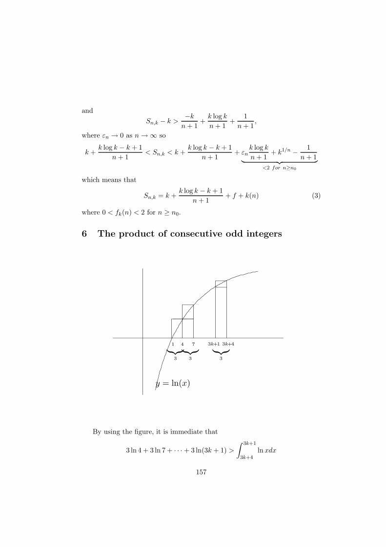
and

Sn,k − k >−kn+ 1

+k log k

n+ 1+

1

n+ 1,

where εn → 0 as n→ ∞ so

k +k log k − k + 1

n+ 1< Sn,k < k +

k log k − k + 1

n+ 1+ εn

k log k

n+ 1+ k1/n − 1

n+ 1︸︷︷︸<2 for n≥n0

which means that

Sn,k = k +k log k − k + 1

n+ 1+ f + k(n) (3)

where 0 < fk(n) < 2 for n ≥ n0.

6 The product of consecutive odd integers

y = ln(x)

1 4 7 3k+1 3k+4

︸︷︷︸︸︷︷︸︸︷︷︸3 3 3

By using the figure, it is immediate that

3 ln 4 + 3 ln 7 + · · · + 3 ln(3k + 1) >

∫ 3k+1

3k+4lnxdx

157

and

3 ln 4 + 3 ln 7 + · · · + 3 ln(3k + 1) <

∫ 3k+4

4lnxdx.

By denoting

P = 1 · 4 · 7 . . . (3k + 1) =

k∏

i=0

(3i+ 1),

we get the double inequality:

1

3

∫ 3k+1

1lnxdx < lnP <

1

3

∫ 3k+4

4lnxdx.

Since ∫lnxdx = x lnx− x+ C,

easy calculation gives

3k + 1

3ln(3k + 1) − k < lnP <

3k + 4

3ln(3k + 4) − k − 4 ln 4,

i.e.

(3k + 1)3k+1

3 e−k < P < (3k + 4)3k+4

3 e−k4−4 < (3k + 4)3k+4

3 e−k. (1)

This is much better than the expected order ≈ (k + 1)2k

k. In the same

manner, by denoting

Q = 1 · 3 · 5 . . . (2k − 1)

one can deduce

1

2

∫ 2k−1

1lnxdx < lnQ <

1

2

∫ 2k+1

3lnxdx,

giving(

2k − 1

e

) 2k−12

< Q <

(2k + 1

2

) 2k+12

. (2)

158

7 On Hadamard’s inequality

1. Let f : [a, b] → R be a continuous, convex function. The classi-cal Hadamard (or ”Jensen-Hadamard”, or ”Hermite-Hadamard”) inequalitiesstate that

(b− a)f

(a+ b

2

)≤∫ b

af(t)dt ≤ (b− a)

[f(a) + f(b)

2

]. (1)

In what follows, we shall improve the left side inequality of (1). Certainapplications for the number e, or the logarithmic mean, will be pointed out.A Hungarian version of this note has been published in 1982 [2].

Our result is based on the following version of Taylor’s theorem:Theorem 1. If f : [x, y] → R, x < y has a continuous nth derivative on

[x, y], and is n+ 1 times differentiable on (x, y), then there exist θ, θ′ ∈ (0, 1)such that

f(y) = f(x) +y − x

1!f ′(x) + · · · + (y − x)n

n!f (n)(x)

+(y − x)n+1

(n+ 1)!f (n+1)(x+ θ(y − x)) (2)

and

f(x) = f(y) +x− y

1!f ′(y) + · · · + (x− y)n

n!f (n)(y)

+(x− y)n+1

(n+ 1)!f (n+1)(y + θ(x− y)). (3)

Proof. We shall give only the proof of (2), since (3) may be proved in acompletely similar way.

Let K be the constant given by the equality

f(y) − f(x) − y − x

1!f ′(x) − · · · − (y − x)n

n!f (n)(x) = (y − x)n+1K,

and consider the application ϕ : [x, y] → R,

ϕ(t) = f(t) +y − t

1!f ′(t) + · · · + (y − t)n

n!f (n)(t) + (y − t)n+1K, t ∈ [x, y].

It is immediate that, ϕ is continuous on [x, y], and differentiable on itsinterior. It is easy to see that

ϕ′(t) =(y − t)n

n!f (n+1)(t) − (n+ 1)(y − t)nK.

159

On the other hand, ϕ(x) = ϕ(y) = f(y), so by the Rolle mean valuetheorem, there exists ξ = x+ θ(y − x), θ ∈ (0, 1), such that ϕ′(ξ) = 0, whichgives

K =1

(n+ 1)!f (n+1)(ξ),

and this finishes the proof of (2).Theorem 2. Let f : [a, b] → R a 2k-times differentiable function, with

f (2k) continuous on [a, b], and with f (2t)(t) > 0 (≥ 0) for all t ∈ (a, b). Thenone has ∫ b

af(t)dt >

(≥)

k∑

p=1

(b− a)2p−1

22p−2(2p − 1)!f (2p−2)

(a+ b

2

). (4)

Proof. Let us consider first the function g :

[a+ b

2, b

]→ R given by

g(s) =

∫ s

af(t)dt,

and apply (2) for x =a+ b

2, y = b, n = 2k. Then we get

∫ b

af(t)dt =

∫ a+b

2

af(t)dt+

b− a

2f

(a+ b

2

)+

(b− a)2

22 · 2! f′(a+ b

2

)+ · · ·+

+(b− a)2k

22k(2k)!f (2k−1)

(a+ b

2

)+

(b− a)2k+1

22k+1(2k + 1)!f (2k)(ξ), (5)

where ξ ∈(a+ b

2, b

). Let us consider similarly h :

[a,a+ b

2

]→ R,

h(s) =

∫ b

sf(t)dt,

and apply (3) for x = a, y =a+ b

2, n = 2k:

∫ b

af(t)dt =

∫ b

a+b

2

f)t)ft+b− a

2f

(a+ b

2

)− (b− a)2

22 · 2! f′(a+ b

2

)+ · · · −

−(b− a)2k

22k(2k)!f (2k−1)

(a+ b

2

)+

(b− a)2k+1

22k+1(2k + 1)!f (2k)(η), (6)

160

where η ∈(a,a+ b

2

).

By adding (5) and (6), and by f (2k)(ξ) > 0 (≥ 0), f (2k)(η) > 0 (≥ 0), weget relation (4).

Corollary. If f (4) is continuous on [a, b] and f (4) > 0 (≥ 0) on (a, b), then

∫ b

af(t)dt > (≥)(b− a)f

(a+ b

2

)+

(b− a)3

24f ′′(a+ b

2

). (7)

This is a consequence of (4) for k = 2.2. Applications1) For all a > 0 one has the double inequality

2a+ 2

2a+ 1<

e(1 +

1

a

)a <

√1 +

1

a. (8)

Proof. Apply (4) for k = 1 (i.e. the left side of (1)) for a > 0, b = a + 1,

f1(t) =1

t, f2(t) = − ln t. Then we get

∫ a+1

a

1

tdt >

2

2a+ 1and

∫ a+1

aln tdt < ln

2a+ 1

2,

and after some elementary calculations, we get (8).Remark. There are many consequences of the double inequality (8). For

example, it easily implies the limit

lima→∞

a

[e−

(1 +

1

a

)a]=e

2.

2) For all a > 0 one has

2a+ 2

2a+ 1e

16(2a+1)2 <

e(1 +

1

a

)a <

√1 +

1

a· e−

13(2a+1)2 . (9)

Proof. Apply the Corollary (i.e. (7)) for the same functions and numbersas in 1). An easy computation yields (9). For some consequences of (9), seee.g. [3].

3) The theorem of finite increments (i.e. the Lagrange mean value the-orem) asserts the existence of an intermediate value θ(f) ∈ (a, b) such that

161

f(b) − f(a) = (b − a)f ′(θ(f)). This θ(f) is not uniquely determined in all

cases. Let e.g. f : [a, b] → R, [a, b] = [−1, 1], f(x) = x3, when θ1(f) =−√

3

3

or θ2(f) =

√3

3. If one assumed, however that f ′ = F is a bijective function,

then clearly θ(f) will be uniquely determined by the relation

θ(f) = F−1

[f(b) − f(a)

b− a

].

Now, as an application of (7), the following will be proved ([4]):Theorem 3. Put F = f ′, and suppose that f is 5-times continuously

differentiable on [a, b], f (5)(t) > 0 on (a, b), and that f ′′(t) < 0 on (a, b). Then

θ(f) < F−1

[F

(a+ b

2

)+

(b− a)2

24F ′′(a+ b

2

)]. (10)

Proof. Clearly F satisfies the conditions of (7), so

∫ b

aF (t)dt > (b− a)F

(a+ b

2

)+

(b− a)3

24F ′′(a+ b

2

).

By the Newton-Leibnitz formula, and after dividing with (b− a), since Fis strictly increasing, we get immediately (10).

For an application of (10), let us consider f(x) = lnx, 0 < a < b. Then

F (x) =1

x, f ′′(x) = − 1

x2< 0, f (5)(x) =

24

x5> 0, so (10) gives

θ(f) <3

8· (a+ b)3

a2 + ab+ b2.

By letting a = 3√x, b = 3

√y in (11), after some elementary transformations,

(11) becomes

L(x, y) =x− y

lnx− ln y<

(3√x+ 3

√y

2

)3

, (12)

where L is the logarithmic mean of 0 < x < y. Inequality (12) is due to T.P.Lin [1]. See also [3] for related results.

References

[1] T.P. Lin, The power mean and the logarithmic mean, Amer. Math.Monthly, 81(1974), 879-883.

162

[2] J. Sandor, On Hadamard’s inequality (Hungarian), Mat. Lapok (Cluj),87(1982), 427-430.

[3] J. Sandor, Some integral inequalities, Elem. Math. (Basel), 43 (1988),177-180.

[4] J. Sandor, On the theorem of finite increments (Hungarian), Mat. Lapok(Cluj), 99(1994), 361-362.

8 On certain inequalities for the number e

The following inequality refines many known relations (see e.g. [3])

2a+ 2

2a+ 1<

e(1 +

1

a

)a <

√1 +

1

a<

2a+ 1

2a, a > 0. (1)

Inequality (1) appeared as an application of Hadamard’s inequality (see[1]). For refinements, with applications, see also [2].

We now prove that (1) will enable us to determine the best constants α > 0and β > 0, such that

1 +α

n≤ e(

1 +1

n

)n ≤ 1 +β

n, n = 1, 2, . . . (2)

Remark that (1) immediately gives that the best β is β =1

2. Indeed, if (2)

is true, then by (1) one must have

2n+ 2

2n+ 1= 1 +

1

2n+ 1< 1 +

β

n,

so n(1 − 2β) < β. This is possible for all n if 1 − 2β ≤ 0, i.e. β ≥ 1

2. On the

other hand, by (1) one has

e(1 +

1

n

)n <2n+ 1

2n= 1 +

1

2n,

i.e. the right side of (2) is true with β =1

2. Therefore, in the right-hand side

we cannot have a sign of equality.

163

Now, if (2) is true for α, by (1) clearly follows 1 +α

n< 1 +

1

2n, so α <

1

2.

However, this doesn’t give necessarily an acceptable value for α.

Another method (which will give again the best β =1

2) is to write (2) is

another form, namely

α ≤ n

e(

1 +1

n

)n − 1

≤ β. (3)

Put

f(x) = x

e(

1 +1

x

)x − 1

, x ≥ 1.

Let

e(x) =

(1 +

1

x

)x

.

It is an easy calculus to deduce that

e′(x) = e(x)

[ln

(1 +

1

x

)− 1

x+ 1

]

and

f ′(x) =

e− e(x) − ex

[ln

(1 +

1

x

)− 1

x+ 1

]

e2(x).

We will show that f ′(x) > 0, or equivalently(

1 +1

x

)x

+ e ln

(1 +

1

x

)x

< e+ex

x+ 1= e

(2x+ 1

x+ 1

).

This may be written in a more acceptable form as(

1 +1

x

)x

e+ ln

(1 +

1

x

)x

<2x+ 1

x+ 1. (5)

First, remark that, by (1) one can write(

1 +1

x

)x

e<

2x+ 1

2x+ 2(∗)

164

and

ln

(1 +

1

x

)x

< 1 +2x+ 1

2x+ 2(∗∗)

by the known inequality ln t ≤ t− 1, t > 0. From (∗), (∗∗) follows relation (5).We have proved that f ′(x) > 0, x > 0. Now this implies

f(n) ≥ f(1) =e

2− 1 for all n = 1, 2, . . .

Therefore, this is the best value of α. Since it is known that

limn→∞

n

[e−

(1 +

1

n

)n]=e

2,

we get

limn→∞

f(n) =1

2,

so β ≥ 1

2, by reobtaining the result obtained in the first part of this note.

All in all, supα =e

2− 1, inf β =

1

2in relation (2). The equality is attained

in the left side (and it is not on the right side).

References

[1] J. Sandor, On Hadamard’s inequality (Hungarian), Mat. Lapok, 8-9(1982), 427-430.

[2] J. Sandor, Some integral inequalities, Elemente der Math. (Basel),43(1988), 177-180.

[3] J. Sandor, On certain inequalities for the number e, Octogon Math. Mag.,10(2002), no.2, 852-853.

9 The Jensen integral inequality

The double inequality

f

(a+ b

2

)≤ 1

b− a

∫ b

af(x)dx ≤ f(a) + f(b)

2(1)

which is valid for all convex functions f : [a, b] → R, is known in the literatureas the Jensen-Hadamard inequalities. Particularly, the right side of (1) is called

165

the Jensen integral inequality. Recently, inequalities (1) has been extended for2k-times (k ≥ 1) differentiable functions ([3], [1]) and various applications ([4],[5], [2]) were given. For a multivariate generalization we quote [2]. Let us nowsuppose that f : [a, b] → R has a strictly increasing derivative on [a, b]. ByLagrange’s mean-value theorem easily follows

f(x) − f(y) < f ′(x)(x− y) for all x, y ∈ [a, b]. (2)

By integrating with respect to x, we get

∫ b

af(x)dx < (b− a)f(y) − y[f(b) − f(a)] + λ = g(y), (3)

where

λ =

∫ b

axf ′(x)dx = bf(b) − af(a) −

∫ b

af(x)dx

and g : [a, b] → R is defined as above. Clearly,

g′(y) = (b− a)f ′(y) − [f(b) − f(a)]

so by the Lagrange mean-value theorem g′(y0) = 0 for some y0 ∈ (a, b). Sincef ′ is strictly increasing, obviously g′(y) > g′(y0) = 0 for y > y0 and g′(y) <g′(y0) = 0 for y < y0. This means that y0 is a minimum-point for the functiong, that is

g(y0) ≤ g(y) for all y ∈ [a, b]. (4)

We can now formulate the following result:Theorem. Let f : [a, b] → R have a strictly increasing derivative on [a, b].

Then

∫ b

af(x)dx <

b− a

2

(f(y0) − y0

[f(b) − f(a)

b− a

]+bf(b) − af(a)

b− a

)(5)

where y0 is defined by the equality

f ′(y0) =f(b) − f(a)

b− a. (6)

For this choose of y = y0, inequality (5) is the strongest.Proof. We apply (3) for y = y0 and then inequality (4) for the function g.

We omit the details.Remark. Clearly, inequality (5) is valid for all y0 ∈ [a, b], but for y0 given

by (6) we get the best result.

166

Corollary. Under the same condition we have:

∫ b

af(x)dx <

b− a

2

[f

(a+ b

2

)+f(a) + f(b)

2

]<b− a

2[f(a) + f(b)]. (7)

Proof. Selecting y =a+ b

2∈ [a, b], by (4) and (5), after a simple compu-

tation we get the first relation in (7). The second inequality is a consequence

of f

(a+ b

2

)<f(a) + f(b)

2which is true, since by the mean-value theorem

f

(a+ b

2

)− f(a) =

b− a

2f ′(c1) < f(b) − f

(a+ b

2

)=b− a

2f ′(c2),

for all c1 < c2.

Applications. 1) Choose f1(x) =1

xand f2(x) = − log x in (5), for 0 <

a < b. Then y0,1 =√ab = G(a, b) = G the geometric mean of a and b;

y0,2 =b− a

log b− log a= L(a, b) = L, the logarithmic mean of a and b. We now

select f3(x) = x log x. Denoting

I = I(a, b) =1

e

(bb

aa

) 1b−a

, a 6= b,

the so-called identric mean of a and b, we can remark that

log I(a, b) =1

b− a

∫ b

alog xdx =

b log b− a log a

b− a− 1.

One gets y0,3 = I(a, b). After some elementary transformations we obtainthe relations

G < L 0, k > 1. Then f ′ is strictly increasing and a simple

calculus shows that

y0 =

(bk − ak

k(b− a)

) 1k−1

.

Relation (5) gives the inequality:

(bk+1 − ak+1

(k + 1)(b − a)

) 1k

>

(bk − ak

k(b− a)

) 1k−1

(9)

167

where b > a > 0 and k > 1. In fact, (9) is valid also for k = 1 in sense that

a+ b

2> lim

k→1

(bk − ak

k(b− a)

) 1k−1

= I(a, b),

after a little limit calculus. This is valid according to the last inequality in (8).We note that, by more difficult arguments it can be proved that (9) is validfor all real k, k 6∈ −1, 0, 1.

3) For f(x) = xex and using the ”exponential mean” ([6])

E(a, b) =beb − aea

eb − ea− 1, a 6= b,

by taking into account of

∫ b

axexdx = (eb − ea)E(a, b)

we can derive from (5):

E(a, b)

(2 + log

(eb − ea

b− a

))<b2eb − a2ea

eb − ea. (10)

References

[1] H. Alzer, A note on Hadamard’s inequality, C.R. Math. Rep. Acad. Sci.Canada, 11(1989), 255-258.

[2] S.S. Dragomir, J.E. Pecaric, J. Sandor, A note on the Jensen-Hadamardinequalities, Rev. d’Anal. Num. Th. Approx., 19(1990), 29-34.

[3] J. Sandor, Some integral inequalities, Elem. Math., 43(1988), 177-180.

[4] J. Sandor, Sur la fonction Gamma, Publ. C.R. Math. Neuchatel, SerieI, 21(1989), 4-7.

[5] J. Sandor, An application of the Jensen-Hadamard inequality, NiuewArch Wisk., (4)8(1990), no.1, 63-66.

[6] J. Sandor, Gh. Toader, On some exponential means, Seminar on Math.Analysis, Preprint no.7, 1990, 35-40.

[7] K.B. Stolarky, The power and generalized logarithmic means, Amer.Math. Monthly, 87(1980), 545-548.

168

10 Generalizations of certain integral inequalities

1. IntroductionLet f : [a, b] → R, a < b, be a (continuous) convex function. The double

inequality

f

(a+ b

2

)≤ 1

b− a

∫ b


2(1)

which is known as the Hadamard (or Jensen-Hadamard) inequalities, has beenrecently intensively studied by some authors. Many applications in differentbranches of Mathematics have been given ([6-12]), and certain extensions,generalizations ([6], [7], [2], [1], [13], [14]) as well as refinements ([2], [3], [4])are know.

The aim of this paper is to obtain certain generalized version of the twosides of (1) for expressions of type

Ep,f(a, b) =

∫ b

ap(x)f(x)dx

∫ b

ap(x)dx

= (Ep,f ) (2)

where p is strictly positive monotone function. A key tool in proof will be theclassical Chebyshev inequality ([5]):

Let f1, f2 : [a, b] → R be monotone in the same sense. Then

1

a− b

∫ b

af1(x)f2(x)dx ≥ 1

b− a

∫ b

af1(x)dx · 1

b− 1

∫ b

af2(x)dx. (3)

If f1 and f2 are monotone in the opposite sense, then the sign of inequalityis reversed in (3). We note that for f1(x) ≡ 1 or f2(x) ≡ 1 one has equality in(3).

Let f be convex, p strictly positive, and f and p monotone in the samesense. Then (3) applied to f1 = f , f2 = p, and with the left side of (1)immediately give

Ep,f ≥ f

(a+ b

2

). (4)

If f is convex and f and p are monotone in the opposite sense, by the sameremark we have

Ep,f ≤ f(a) + f(b)

2. (5)

We will obtain results of type (4) and (5) or refinements, for convex func-tions f without monotonicity properties. In what follows, p will be always astrictly positive function.

169

2. ResultsFirst prove thatTheorem 1. Let f be a convex function. Then

Ep,f ≥ f(A) + f ′+(A)Cp (6)

where A =a+ b

2and Cp = Cp(a, b). If p is increasing, then Cp ≥ 0, while for

decreasing p one hasCp ≤ 0. (7)

Thus, when f ′+(A) ≥ 0 and p increasing, (4) holds true. If f ′+(A) ≤ 0 andp is decreasing, the same inequality (4) is valid.

Proof. Since f is convex on [a, b], it is known that

f(x) − f(A) ≥ f ′+(A)(x −A). (8)

Multiplying both sides of (8) with p(x) > 0 and integrating term-by-term,we get

∫ b

ap(x)f(x)dx− f(A)

∫ b

ap(x)dx ≥ f ′+(A)

∫ b

ap(x)(x−A)dx. (9)

Let

Kp =

∫ b

ap(x)(x−A)dx.

We shall prove that for increasing p one has Kp ≥ 0. Indeed, since f1(x) =p(x) and f2(x) = x−A are increasing, by (3)

Kp ≥ 1

b− a

∫ b

ap(x)dx

∫ b

a(x−A)dx = 0,

by

∫ b

a(x−A)dx = 0. Thus Cp ≥ 0. When p decreases, an analogous proof can

be made, giving (7).Remark. When f is convex with f ′+(A) ≥ 0, one obtains a refinement of

(4),Ep,f ≥ f(A) + f ′+(A)Ep,f2 ≥ f(A), (10)

where f2(x) = x−A (see the proof of Theorem 1). If f is strictly convex withf ′+(A) > 0, then (10) holds with strict inequalities.

Application. Set p(x) = expx and denote

E = E(a, b) =beb − aea

eb − ea− 1, a < b

170

the so called ”exponential mean” of a and b (see [15], [16]). Since

E =

∫ b

aexxdx

∫ b

aexdx

from (10) we get

Eexp,f ≥ f(A) + f ′+(A)(E −A) ≥ f(A), (11)

where exp denotes the exponential function. We note that the right side of(11) implies the inequality

E > A (12)

with f(x) = x. Let f(x) = x2 in (11). By

∫ b

ax2exdx

∫ b

aexdx

=ebb2 − eaa2

eb − ea − 2E

(which gives a new exponential mean), we obtain the inequality

ebb2 − eaa2

eb − ea> 2E(A+ 1) −A > A2 + 2E. (13)

We now improve relation (5).Theorem 2. Let f be convex with f(b) ≥ f(a). If p is a decreasing func-

tion, then

Ep,f ≤ f(a) +f(b) − f(a)

b− a

∫ b

a(x− a)p(x)dx ≤ f(a) + f(b)

2. (14)

The same is valid when f(b) ≤ f(a) and p is increasing.Proof. Since f is convex on [a, b], one has

f(x) ≤ f(a) +f(b) − f(a)

b− a(x− a) = K(x) (15)

which means that f(x) ≤ K(x), where intuitively the set (x, y) : x ∈[a, b], y = K(x) represents the line segment joining the points (a, f(a)),

171

(b, f(b)) of a graph of f . Multiplying both sides of (15) with p(x) > 0 andintegrating, one gets

∫ b

ap(x)f(x)dx ≤

(∫ b

ap(x)dx

)f(a) +

f(b) − f(a)

b− a

∫ b

a(x− a)p(x)dx. (16)

Since p(x) decreases, inequality (3) holds with reversed sign of inequality,thus

∫ b

a(x− a)p(x)dx ≤ 1

b− a

∫ b

a(x− a)dx

∫ b

ap(x)dx =

b− a

2

∫ b

ap(x)dx.

By f(b) − f(a) ≥ 0 and taking into account of (16), we obtain relation(14). This holds true also when f(b) ≤ f(a) and p is increasing.

Remarks. 1) The function f :

[−1

2, 1

]→ R, f(x) = x2k (k ≥ 1 integer)

is convex with f(1) = 1 > f

(−1

2

)= 2−2k, without being monotone. Thus

for an arbitrary strictly positive, decreasing function p one has

∫ 1

− 12

x2kp(x)dx

∫ 1

− 12

p(x)dx

≤ 2−2k +(22k − 1)2−2k+1

3

∫ 1

− 12

(x+

1

2

)p(x)dx

≤ (22k + 1)2−2k−2. (17)

With analogous proof we can say that, when f is concave, f(b) ≥ f(a),and p is increasing (or f(b) ≤ f(a) but p decreases) the inequalities in (14)are reversed. For a generalization, the positivity of f is needed:

Theorem 3. Let f be positive and convex with f(b) ≥ f(a). If n ≥ 1 is apositive integer, and p is decreasing, then

Ep,fn ≤n∑

k=0

(n

k

)fk(a)

(f(b) − f(a)

b− a

)n−k ∫ b

a(x− a)n−kp(x)dx

≤n∑

k=0

(n

k

)fk(a)(f(b) − f(a))n−k

n− k + 1. (18)

(Here fk(a) = (f(a))k).Proof. Since f is positive, by (15) and Newton’s binomial theorem we

immediately obtain the middle inequality of (18). The last inequality followsby (3) (reversed inequality) and some simple computations.

172

Remark. When p(x) ≡ 1, the condition f(b) ≥ f(a) is not necessary. (Wenote that for this p in Theorem 1,2 only the convexity of f is needed). In thiscase for n = 2 one obtains the relation

1

b− a

∫ b

af2(x)dx ≤ 1

3(f2(a) + f(a)f(b) + f2(b)) (19)

which appeared (with applications) also in [12]. A generalization of the abovetype can be proved for concave functions, too:

Theorem 4. Let f be positive and concave and n ≥ 1 a positive integer.Then

Ep,fn ≤n∑

k=0

(n

k

)fn−k(A)(f ′+(A))k

∫ b

a(x−A)kp(x)dx. (20)

If f ′+(A) ≥ 0 (where A =a+ b

2) and p is decreasing, the right side of (20)

can be majored by

n∑

k=0

(n

k

)fn−k(A)(f ′+(A))k · 2−k−1 1 + (−1)k

k + 1(b− a)k. (21)

Proof. One has (f being concave) 0 < f(x) ≤ f(A) + f ′+(A)(x−A) so byNewton’s binomial theorem one obtains (after multiplication with p(x) > 0and integration) relation (20). For (21) remark that (3) can be used (with”≤”). Since

1

b− a

∫ b

a(x−A)kdx = 2−k−1 1 + (−1)k

k + 1(b− a)k

(easy calculation) we get the desired result.Remark. For p(x) ≡ 1, n = 2, f positive and concave one obtains the

inequality1

b− a

∫ b

af2(x) ≤ f2(A) + (f ′+(A))2

(b− a)2

12. (22)

References

[1] H. Alzer, A note on Hadamard’s inequalities, C.R. Math. Rep. Acad.Sci. Canada, 11(1989), 155-258.

[2] S.S. Dragomir, J.E. Pecaric, J. Sandor, A note on the Jensen-Hadamardinequalities, Rev. d’Anal. Num. Th. Approx., 19(1990), 19-34.

173

[3] S.S. Dragomir, Two mappings in connection to Hadamard’s inequalities,J. Math. Anal. Appl., 167(1992), 49-56.

[4] S.S. Dragomir, D.M. Milosevic, J. Sandor, On some refinements ofHadamard’s inequalities and applications, Univ. Beograd Publ. Elekt.Fak., Ser. Mat., 4(1993), 3-10.


[6] J. Sandor, On Hadamard’s inequality (Hungarian), Matematikai Lapok(Cluj), 87(1982), 427-430.


[8] J. Sandor, Remark on a function which generalizes the harmonic series,C.R. Bulg. Acad. Sci., 41(1988), 19-21.

[9] J. Sandor, Sur la fonction Gamma, C.R.M.P. Neuchatel, Serie I, Fasc.21, 1989, 4-7.

[10] J. Sandor, Inequalities for means, Proc. 3-th Symposium of Math. andAppl., 1989, Timisoara, 87-90.

[11] J. Sandor, An application of the Jensen-Hadamard inequality, NiuewArch. Wiskunde, (4)8(1990), 63-66.


[13] J. Sandor, On the Jensen-Hadamard inequality, Studia Univ. Babes-Bolyai, 36(1991), 9-15.

[14] J. Sandor, On certain extensions of the Jensen-Hadamard inequalities,submitted.

[15] J. Sandor, Gh. Toader, On some exponential means, Seminar Math.Analysis, Babes-Bolyai Univ., Preprint nr.7, 1990, 35-40.

[16] Gh. Toader, An exponential mean, Seminar Math. Analysis, Babes-Bolyai Univ., Preprint nr.5, 1988, 51-54.

174

11 The Chebyshev integral inequality

let (ai), (bi), (pi), i = 1, n, be sequences of real numbers, such that

(ai − aj)(bi − bj) ≥ 0, i, j = 1, n (1)

pi ≥ 0. (2)

Then pipj(ai −aj)(bi − bj) ≥ 0 for all i, j and letting∑

i,j

in this inequality,

after multiplication, we get:(

n∑

i=1

pi

)(n∑

i=1

piaibi

)

≥(

n∑

i=1

piai

)(n∑

i=1

pibi

)

. (3)

This is weighted Chebyshev inequality for sequences. An example for (1)is when (ai) and (bi) are syncrone sequences (i.e. having the same type ofmonotonity). Let (1) be replaced by

(ai − aj)(bi − bj) ≤ 0, i, j = 1, n. (1′)

In this case one has, by a similar proof(

n∑

i=1

pi

)(n∑

i=1

piaibi

)≤(

n∑

i=1

piai

)(n∑

i=1

pibi

). (3′)

An example of (1′) is when (ai), (bi) are asyncrone sequences, i.e. whenthey have different type of monotonity.

Let now p, f, g : [a, b] → R be real variable functions, such that p ≥ 0 isintegrable and f, g are monotone on [a, b]. Then it is well-known that f, g areintegrable, too.

Let ∆ = a = x0 < · · · < xi−1 < xi < · · · < xn = b be an arbitrarydivision of [a, b] and let

σ∆(f, ξ) =

n∑

i=1

f(ξi)(xi − xi−1)

be the Riemann-sum associated to f , where ξ = (ξ1, . . . , ξn) and ξi ∈ [xi−1, xi]are arbitrary.

Now, let f, g be syncrone functions on [a, b] (i.e. having the same type ofmonotonity) and put ai = f(ξi), bi = g(ξi), pi = p(ξi)(xi − xi−1) in (3). Onegets:

n∑

i=1

p(ξi)(xi − xi−1)n∑

i=1

p(ξi)g(ξi)(xi − xi−1) ≥

175

≥n∑

i=1

p(ξi)f(ξi)(xi − xi−1)

n∑

i=1

p(ξi)g(ξi)(xi − xi−1). (4)

Now, letting ‖∆‖ = supxi−xi−1 → 0 in (4), since the occurring Riemannsums have a limit equal to the integral of the corresponding function, we get:

∫ b

ap(x)dx

∫ b

ap(x)f(x)g(x)dx ≥

∫ b

ap(x)f(x)dx

∫ b

ap(x)g(x)dx. (5)

This is Chebyshev’s integral inequality with weights for syncrone functions.When the functions f, g are asyncrone on [a, b], we get from (3′):

∫ b

ap(x)dx

∫ b

ap(x)f(x)g(x)dx ≤

∫ b

ap(x)f(x)dx

∫ b

ap(x)g(x)dx (6)

the Chebyshev inequality for asyncrone sequences. Inequalities of type (3), (4)are very important in many parts of Mathematics ([1]). For applications inthe Theory of Means and Number Theory, we quote [2], [3], [4], [5], [6].

Let now f, g be syncrone functions, and consider the function defined byh(t) = g(a + b − t), t ∈ [a, b]. Then clearly f, h are asyncrone functions, andapplying (6) for (p, f, g) := (p, f, h) one gets

∫ b

ap(x)dx

∫ b

ap(x)f(x)g(a + b− x)dx ≤

≤∫ b

ap(x)f(x)dx

∫ b

ap(x)g(a+ b− x)dx. (7)

Let us now suppose that p has the following property:

p(a+ b− x) = p(x), x ∈ [a, b]. (8)

Then, by the substitution a+ b− x = t one gets

∫ b

ap(x)g(a + b− x)dx =

∫ b

ap(t)g(t)dt,

and applying (5), by taking into account of (7), we get the following result:Theorem. Let f, g : [a, b] → R be two syncrone functions and let p :

[a, b] → R be a nonnegative integrable function such that (8) is true. Then

∫ b

ap(x)dx

∫ b

ap(x)f(x)g(a + b− x)dx ≤

∫ b

ap(x)f(x)dx

∫ b

ap(x)g(x)dx

176

≤∫ b

ap(x)dx

∫ b

ap(x)f(x)g(x)dx. (9)

Remark. When p(x) ≡ 1, (8) is true. But let p(x) = cos x, [a, b] =[−π2,π

2

]. Then by cos(−x) = cos x, (8) is again true. Here cos x ≥ 0 on

[−π2,π

2

]. These two cases, give the double-inequalities

(b− a)

∫ b

af(x)g(a+ b− x)dx ≤

∫ b

af(x)dx

∫ b

ag(x)dx

≤ (b− a)

∫ b

af(x)g(x)dx (10)

2

∫ π

2

−π

2

cos xf(x)g(−x)dx ≤∫ π

2

−π

2

cosxf(x)g(x)dx

∫ π

2

−π

2

cos xg(x)dx

≤ 2

∫ π

2

−π

2

cos xf(x)g(x)dx (11)

where, in both cases f, g are syncrone functions.

References

[1] G.H. Hardy, J.E. Littlewood, G. Polya, Inequalities, Oxford, 1934.

[2] J. Sandor, On Jordan’s arithmetical function. Math. Student, 52(1984),91-96.

[3] J. Sandor, On certain integral inequalities, Octogon Math. Mag., 5(1997), 29-34.

[4] J. Sandor, On means generated by derivatives of functions, Int. J. Math.E. Sci. Tech., 28(1997), 146-148.

[5] J. Sandor, Gh. Toader, Some general means, Czechoslovak Math. J.,49(124)(1999), 53-62.

[6] J. Sandor, Inequalities for generalized convex functions with applications,II, Studia Univ. Babes-Bolyai Math., XLVI, 2001, 79-92.

177

12 On Fink’s inequality

The following interesting inequality is due to A.M. Fink [1]:Theorem 1. If f > 0 and log f is convex on R, then

∫ 1

−1f(x+ vt) cos

πt

2dt ≤ 2

π(f(x+ v) + f(x− v)), x, v ∈ R. (1)

The aim of this note is to prove that relation holds true if f is convex onR.

Lemma. If g : I → R is a strictly positive, log-convex function, then it isconvex in I (real interval).

Proof. If g : I → R (I ⊂ R, interval) is a strictly positive, log-convexfunction, then

log g(λa+ (1 − λ)b) ≤ λ log g(a) + (1 − λ) log g(b)

for all λ ∈ [0, 1]; a, b ∈ I, implying

g(λa+ (1 − λ)b) ≤ (g(a))λ(g(b))1−λ.

By Holder’s inequality (see e.g. [2]) one has

(g(a))λ(g(b))1−λ ≤ λg(a) + (1 − λ)g(b),

since λ+ (1 − λ) = 1, λ ≥ 0. Thus, g is convex.To prove (1) for convex f , first note that

I =

∫ 1

−1f(x+ vt) cos

πt

2dt =

∫ 1

0(f(x+ vt) + f(x− vt)) cos

πt

2dt. (2)

Put

gx,v(t) = f(x+ vt) + f(x− vt), t ∈ [0, 1]. (3)

Now, since

x± vt =

(1 + t

2

)(x± v) +

(1 − t

2

)(x∓ v),

by convexity of f one can write

gx,v(t) ≤1 + t

2f(x+ v) +

1 − t

2f(x− v) +

1 + t

2f(x− v) +

1 − t

2f(x+ v)

178

= f(x+ v) + f(x− v), t ∈ [0, 1].

So by (2) we have

I ≤ (f(x+ v) + f(x− v))

∫ 1

0cos

πt

2dt =

2

π(f(x+ v) + f(x− v)).

Equality occurs only when gx,v is linear. Then from (3) it follows that fmust be a constant. The given proof shows that the following generalizationof (1) is valid.

Theorem 2. If f is convex function on R, and c is a nonnegative, evenfunction on [−1, 1], then

∫ 1

−1f(x+ vt)c(t)dt ≤ f(x+ v) + f(x− v)

2

∫ 1

−1c(t)dt, x, v ∈ R.

References

[1] A.M. Fink, Two inequalities, Univ. Beograd Publ. Elektrotehn. Fak.,Ser. Mat., 6(1995), 48-49.


13 An extension of Ky Fan’s inequalities

Let xk, k = 1, n, be positive real numbers. The arithmetic respectivelygeometric means of xk are

A = A(x1, . . . , xn) =x1 + · · · + xn

n,

G = G(x1, . . . , xn) = n√x1 . . . xn.

Let f : I → R (I interval), and suppose that xk ∈ (a, b). Define thefunctional arithmetic, respectively geometric ”means” by

Af = Af (x1, . . . , xn) =f(x1) + · · · + f(xn)

n

andGf = Gf (x1, . . . , xn) = n

√f(x1) . . . f(xn).

Clearly, Af and Gf are means in the usual sense, if minx1, . . . , xn ≤Af ≤ maxx1, . . . , xn and minx1, . . . , xn ≤ Gf ≤ maxx1, . . . , xn. For

179

example, when I = (0,+∞) and f(x) = x, Af ≡ A, Gf ≡ G; when I = (0, 1)and f(x) = 1 − x, Af = A′, Gf = G′, are indeed means in the above sense.

The following famous relations are well-known:

G ≤ A for xk > 0, k = 1, n (1)

G

G′ ≤A

A′ for xk ∈(

0,1

2

]. (2)

The first is the arithmetic-geometric inequality, while the second is theKy-Fan inequality (see e.g. [2], [3], [4]). Now, even if Af and Gf are not meansin the usual sense, the following extension of (2) may be true:

G

Gf≤ A

Af. (3)

This inequality (with other notations) is stated in OQ.633, in [1]. We nowprove (3) for certain particular f .

Theorem. Let id : R → R, id(x) = x and suppose that f : I → R satisfies

the following conditions: f and lnid

fare concave functions. Then inequality

(3) holds true.

Proof. By concavity of lnid

fone can write:

ln

x1 + · · · + xn

n

f

(x1 + · · · + xn

n

) ≥[ln

x1

f(x1)+ · · · + ln

xn

f(xn)

]1

n,

i.e.

lnA

f(A)≥ ln

G

Gf.

ThereforeG

Gf≤ A

f(A). (4)

Now, since f is concave, one has

Af =f(x1) + · · · + f(xn)

n≤ f

(x1 + · · · + xn

n

)= f(A),

and by (4) this gives (3).

180

Remark 1. Let I =

(0,

1

2

]and f(x) = 1 − x, then g(x) = ln

x

1 − xhas a

derivative

g′(x) =1

x+

1

1 − x,

so

g′′(x) = − 1

x2+

1

(1 − x)2=x2 − (1 − x)2

x2(1 − x)2=

2x− 1

x2(1 − x)2≤ 0.

Therefore f and lnid

fare concave functions, and (4) gives Ky Fan’s in-

equality (2). One has equality for xk =1

2, k = 1, n.

Remark 2. There are many functions f : I → R such that f and lnid

fare simultaneously concave. Put e.g. f(x) = lnx. Then

g(x) = lnx

lnx= lnx− ln lnx.

One has

g′′(x) =− ln2 x+ lnx+ 1

x2 ln2 x≤ 0

if lnx ≥ 1 +√

5

2, i.e. x ≥ e

1+√

52 = x0. (Take I = [x0,+∞)).

Remark 3. Without concavity of f , holds true (4).

References

[1] M. Bencze, OQ.633, Octogon Math. Mag., 9(2001), no.1, 679-680.

[2] J. Sandor, On an inequality of Ky Fan, III, Intern. J. Math. Ed. Sci.Tech., 32(2001), no.1, 133-160.

[3] J. Sandor, T. Trif, A new refinement of the Ky Fan inequality, Math.Ineq. Appl., 2(1999), no.4, 529-533.

[4] E. Neumann, J. Sandor, On the Ky Fan inequality and related inequali-ties, I, Math. Ineq. Appl., 5(2002), 49-56; for II, see Bull. Austral. Math.Soc. (to appear).

181

14 A converse of Ky Fan’s inequality

Let xi ∈(

0,1

2

], i = 1, n, and let An, Gn,Hn denote the arithmetic, geo-

metric, resp. harmonic means of these numbers. Put A′n, G

′n,H

′n for the corre-

sponding means of the numbers 1− xi. The famous inequality of Ky Fan (see[1]) states that

Gn

G′n

≤ An

A′n

. (1)

Suppose that m > 0 and xi ∈[m,

1

2

]. Then the following converse of (1)

is true:Theorem.

An

A′n

≤ Gn

G′n

exp

[(An −Gn)

1

m(1 −m)

]. (2)

Proof. We shall obtain a slightly stronger relation. Let us define

f(x) =x

1 − xexp

(1 − x

m

) 1

1 −m

, where x ∈

[m,

1

2

].

Thenf ′(x)f(x)

=1

x(1 − x)− 1

m(1 −m)≤ 0 for x ≥ m,

since the function g(x) = x(1 − x) is strictly increasing on

[0,

1

2

]. Thus the

function f is non-increasing on

[m,

1

2

]. Suppose that m ≤ x1 ≤ x2 ≤ · · · ≤

xn ≤ 1

2. Then, since m ≤ Gn ≤ An, we have f(An) ≤ f(Gn) so that

An

A′n

≤ Gn

1 −Gnexp

[(An −Gn)

1

m(1 −m)

]. (3)

This is slightly stronger than (2), since 1 − Gn ≥ G′n. This follows by

the well-known inequality n

√(1 + a1) . . . (1 + an) ≥ 1 + n

√a1 . . . an (see e.g.

[2], Theorem 64, p.61), which for ai =ui

vi, ui, vi > 0, implies n

√u1 . . . un +

n√v1 . . . vn ≤ n

√(u1 + v1) . . . (un + vn). Apply then this inequality to ui = xi,

vi = 1 − xi in order to get Gn +G′n ≤ 1, xi ∈ (0, 1). Thus (2) follows.

182

References

[1] E.F. Beckenbach, R. Bellman, Inequalities, Springer Verlag, 1961.

[2] G.H. Hardy, J.E. Littlewood, G. Polya, Ineqialities, Cambridge Univ.Press, Second Reprinted ed., 1964.

15 A refinement of Gn + G′n ≤ 1

Suppose that xi ∈ (0, 1), i = 1, 2, . . . , n, and let Gn = Gn(xi) denote thegeometric mean of xi, i.e. Gn = n

√x1 . . . xn. Put

G′n = n

√(1 − x1) . . . (1 − xn).

The well-known inequality

n√u1 . . . un + n

√v1 . . . vn ≤ n

√(u1 + v1) . . . (un + vn), ui, vi ≥ 0

applied to ui = xi, vi = 1 − xi implies the relation Gn + G′n ≤ 1 (see also

[2]). By using the optimization theory of concave functions, in what followswe shall prove the following refinement:

Theorem. (Gn +G′n)n ≤ (Gn−1 +G′

n−1)n−1 ≤ 1 for all n ≥ 2.

Proof. Let us consider the application f : (0, 1) → R, defined by

f(x) = (x1 . . . xn−1x)1/n + [(1 − x1) . . . (1 − xn−1)(1 − x)]1/n.

We have

f ′(x) =1

n(x1 . . . xn−1)

1xx

1n−1 − 1

n[(1 − x1) . . . (1 − xn−1)]

1n (1 − x)

1n−1,

so f ′(x) = 0 iff x = x0 =Gn−1

Gn−1 +G′n−1

.

Since

f ′′(x) =1

n

(1

n− 1

)(x1 . . . xn−1)

1nx

1n−2

+1

n

(1

n− 1

)[(1 − x1) . . . (1 − xn−1)]

1n (1 − x)

1n−2 ≤ 0

we observe that f is a concave function. It is well known (see e.g. [1]) thatthen x0 must be a maximum point on (0, 1), implying f(xn) ≤ f(x0). Aftersome simple calculations this gives

Gn +G′n ≤ (Gn−1 +G′

n−1)n−1

n ,

i.e. the first relation of the Theorem.

183

References

[1] A.W. Roberts, D.E. Varberg, Convex functions, Academic Press, NewYork and London, 1973.

[2] J. Sandor, On an inequality of Ky Fan, Babes-Bolyai Univ. Preprint nr.7,29-34.

16 On Alzer’s inequality

H. Alzer [1] discovered the following result:Theorem. If r is a positive real number and n is a positive integer, then

n

n+ 1≤(

(n+ 1)

n∑

i=1

ir/n

n+1∑

i=1

ir

)1/r

. (1)

We will obtain a proof based on mathematical induction and Cauchy’smean value theorem of differential calculus. More precisely, we will prove that(1) holds with strict inequality.

Proof. Let us denote

Sr(n) = 1r + 2r + · · · + nr, n = 1, 2, . . . , r > 0.

Then, since Sr(n + 1) = Sr(n) + (n + 1)r, it is immediate that inequality(1) is equivalent to

Sr(n) ≥ nr+1(n+ 1)r/((n + 1)r+1 − nr+1). (2)

We shall deduce this inequality via mathematical induction. For n = 1 onehas 1 ≥ 2r/(2r+1 − 1) which is true by 2r ≥ 1, r > 0. Now, accepting (2) forn, we try to obtain it for n+ 1. By Sr(n+ 1) = Sr(n) + (n+ 1)r, it is easy tosee that the induction step (after dividing by (n+ 1)r) can be written as

(n + 2)r+1 − (n+ 1)r+1

(n+ 1)r+1 − nr+1≥(n+ 2

n+ 1

)r

. (3)

Let us consider the functions f, g : [n, n+ 1] → R defined by

f(x) = (x+ 1)r+1, g(x) = xr+1, x ∈ [n, n+ 1].

By Cauchy’s mean-value theorem one has

[f(n+ 1) − f(n)]/[g(n + 1) − g(n)] = f ′(ξ)/g′(ξ),

184

where ξ ∈ (n, n+ 1), so

(n+ 2)r+1 − (n+ 1)r+1

(n+ 1)r+1 − nr+1=

(ξ + 1)r

ξr=

(1 +

1

ξ

)r

. (4)

By 1/ξ > 1/(n + 1) in (4), we have

(1 + 1/ξ)r > (1 + 1/(n + 1)) =

(n+ 2

n+ 1

)r

,

implying relation (3). This finishes the proof of (2), and thus of the theorem,with strict inequality (see also [2]).

References

[1] H. Alzer, On an inequality of H. Minc and L. Sathre, J. Math. Anal.Appl., 179(1993), 396-402.

[2] J. Sandor, On an inequality for Alzer, J. Math. Anal. Appl., 192(1995),1034-1035.

185

186

Chapter 5

Euler gamma function

”... Mathematics compares the most diverse phenomena and discovers thesecret analogies that unite them.”

(Joseph Fourier)

”... Euler’s integral appears everywhere and is inextricably bound to a hostof special functions. Its frequency and simplicity make it fundamental.”

(Ph. J. Davis)

187

1 A limit involving the Gamma function and theLalescu sequence

Let Lk = k+1√

(k + 1)! − k√k!. We will compute

limn→∞

1

n

n∑

k=1

(Γ(1 + Lk))1/Lk ,

where Γ is the Euler gamma function. Put xn = (Γ(1 + Ln))1/Ln . It is well-

known that Ln → 1

eas n→ ∞ (Traian Lalescu sequence). Since the Γ-function

is continuous in (0,+∞), it follows that

xn →(

Γ

(1 +

1

e

))e

=

[1

eΓ

(1

e

)]e

.

Now the following theorem is well-known:

If xn → a, n → ∞, thenx1 + x2 + · · · + xn

n→ a. Therefore the proposed

limit has a value

[1

eΓ

(1

e

)]e

.

2 On a sequence containing the Gamma function

Let 0 < x1 < x2 < · · · < xn < . . . , and (yn) be defined by

yn =n∑

k=1

Ψ(xk) − ln Γ(xn) (1)

where Ψ(x) =Γ′(x)Γ(x)

, with Γ and Ψ the gamma, respectively digamma func-

tions.Generally, the sequence (yn) is not convergent. Indeed, suppose that (xn)

is convergent, having a limit limn→∞

xn = x0 6= a, where a ∈ (1, 2) is the single

positive root of Γ′(x) = 0. Then (yn) is divergent.Indeed, yn+1−yn = Ψ(xn+1)−[ln Γ(xn+1)−ln Γ(xn)] and since Γ,Ψ are con-

tinuous; if (yn) could be convergent, we would obtain: 0 = Ψ(x0)− [ln Γ(x0)−ln Γ(x0)] = Ψ(x0) so Γ′(x0) = 0, contradiction with the made assumption.

Let us now suppose that 0 < xn+1 − xn ≤ 1. Then

yn+1 − yn = Ψ(xn+1) − [ln Γ(xn+1) − ln Γ(xn)].

188

Here

ln Γ(xn+1) − ln Γ(xn) = (ln Γ′)(ξ)(xn+1 − xn) = Ψ(ξ)(xn+1 − xn),

by the Lagrange mean-value theorem. Since it is well known that ln Γ is a con-vex function on (0,+∞), the digamma function Ψ will be strictly increasing,so

ln Γ(xn+1) − ln Γ(xn) < Ψ(xn+1)(xn+1 − xn) ≤ Ψ(xn+1),

by the accepted assumption. This implies yn+1 − yn > 0, i.e. (yn) is a strictlyincreasing sequence. Thus yn > yn−1 > · · · > y1, and (yn) will be boundedbelow. In any case, (yn) will have a limit, but this limit may be +∞, if it isnot bounded above. By supposing that Ψ(x1) + · · · + Ψ(xn) − ln Γ(xn) < K(K constant), for all n ≥ n0, the sequence (yn) will be convergent.

3 The product of consecutive factorials

We will evaluate

n∏

k=1

k!, or in fact

(n∏

k=1

k!

)=

n∑

k=1

ln k! =

n∑

k=1

ln Γ(k + 1).

Now, the function g(x) = ln Γ(x) is known to be strictly convex and strictlyincreasing for x ≥ 2. By area considerations

g(3) + · · · + g(k) <

∫ k+1

3ln Γ(x)dx < g(4) + · · · + g(k + 1).

Therefore

ln 2 +

∫ n+1

3ln Γ(x)dx < g(3) + · · · + g(n + 1)

=

n∑

k=1

ln Γ(k + 1) <

∫ n+1

3ln Γ(x)dx+ lnn! (1)

Now, it is well-known the asymptotic expansion of ln Γ(x) ([1]):

ln Γ(x) =

(x− 1

2

)lnx− x+ ln

√2π

189

+n−1∑

i=1

B2i

2i(2i − 1)x2k−1+O

(1

x2n−1

)(2)

where (B2i) are the Bernoulli numbers. This improves the Stirling formula

n! ∼√

2πn · nne−n, n→ ∞. (3)

Now, since

∫x lnxdx =

x2 lnx

2− x2

4,

∫lnxdx = x lnx− x

and

ln(n+ 1) = lnn+1

n+O

(1

n

),

from (1), (2), (3) one can deduce

n∑

k=1

ln k! =n2 lnn

2+ n lnn− 3

4n2 +

1

4lnn+ (ln

√2π − 1) + n+ C + o(1).

References

[1] E.T. Whittaker, G.N. Watson, A course in modern analysis, CambridgeUniv. Press, 1969.

4 On Γ(kn)

1. Euler’s Gamma function is defined for x > 0 by

Γ(x) =

∫ ∞

0e−ttx−1dt.

The following relations are well-known:

Γ(1) = 1, Γ(x+ 1) = xΓ(x) (1)

Γ(x) = limn→∞

n!nx

x(x+ 1) . . . (x+ n)(Euler) (2)

Γ(x)Γ(1 − x) =π

sinπx, x ∈ (0, 1) (Gauss) (3)

Γ(x)Γ

(x+

1

2

)=

√π

22x−1Γ(2x) (Legendre) (4)

190

Γ

(1

2

)=

√π, Γ

(n+

1

2

)=

(2n − 1)!!

2n

√π (5)

where (2n− 1)!! = 1 · 3 . . . (2n− 1), etc., see e.g. [1].From (2) we obtain

Γ(2n) =22n−1

√π

Γ(n)Γ

(n+

1

2

), n ∈ N,

and similarly one can deduce a formula for Γ(3n), namely

Γ(3n) =33n− 1

2

2πΓ(n)Γ

(n+

1

2

)Γ

(n+

2

3

).

We will consider a generalization, namely the determination of Fk(n) with:

Γ(kn) = Fk(n)Γ(n)Γ

(n+

1

k

). . .Γ

(n+

k − 1

k

). (6)

We shall prove that

Fk(n) =kkn− 1

2

(2π)(k−1)/2(7)

(due to Gauss), by an elementary method.2. First we show that:

Γ

(1

k

)Γ

(2

k

). . .Γ

(k − 1

k

)=

(2π)(k−1)/2

√π

. (8)

Indeed, by denoting the product in (8) with P , by (3) one can write:

P 2 =

[Γ

(1

k

)Γ

(1 − 1

k

)][Γ

(2

k

)Γ

(1 − 2

k

)]. . .

[Γ

(k − 1

k

)Γ

(1

k

)]

=πk−1

n−1∏

k=1

sinkπ

n

.

But it is well known that

n−1∏

k=1

sinkπ

n=

n

2n−1,

so (8) follows.

191

Let us define the function

g(x) =

kkxΓ(x)Γ

(x+

1

k

). . .Γ

(x+

k − 1

k

)

kΓ(kx), x > 0. (9)

By applying Euler’s formula (2) one has

g(x) =

kkxk−1∏

i=0

limm→∞

m!mx+i/k

(x+

1

k

)(x+

i

k+ 1

). . .

(x+

i

k+m

)

k limm→∞

1 · 2 · 3 . . . (mk)(mk)kx

(kx)(kx + 1) . . . (kx+mk)

= limm→∞

(m!)mkx+ k−12 kmk

(km)!(km)kx

which is independent of x. So g is a constant (of x); implying for example

g(x) = g

(1

k

). By the definition of g (see (9)) one can write

g

(1

k

)=

Γ

(1

k

)Γ

(2

k

). . .Γ

(k − 1

k

)Γ(1)

Γ(1)=

(2π)(k−1)/2

√π

,

by (8). Therefore, we have obtained that:

Γ(kx) =kkx− 1

2

(2π)(k−1)/2Γ(x)Γ

(x+

1

k

). . .Γ

(x+

k − 1

k

), x > 0. (10)

Particularly, for x = n, for Fk(n) in (6) we get relation (7).

5 On a limit for the quotients of Gamma functions

Let Γ(x) =

∫ ∞

0e−ttx−1dt, x > 0 be the Euler gamma function. The follow-

ing asymptotic result is known as the Stirling formula for the gamma function([1])

Γ(x+ 1) =√

2πx(xe

)x[1 +

1

12x+O

(1

x2

)], x > 0. (1)

192

1. Letting x → ax and x → bx (x > 0, a, b > 0) in (1) one obtainssuccessively

[Γ(ax+ 1)]1x = (2πax)

1x

(axe

)a[1 +

1

12ax+O

(1

x2

)] 1x

(2)

[Γ(bx+ 1)]1x = (2πbx)

1x

(bx

e

)b [1 +

1

12bax+O

(1

x2

)] 1x

(3)

(for fixed a, b > 0). From (2) and (3) one obtains

[Γ(bx+ 1)

Γ(ax+ 1)

] 1x

=

(b

a

) 1x

(b

e

)b ( ea

)axb−a

[1 +

1

12bx+O

(1

x2

)] 1x

[1 +

1

12ax+O

(1

x2

)] 1x

. (4)

Clearly[1 +

1

12ax+O

(1

x2

)] 1x

→ 1

as x → ∞ and

(b

a

) 1x

→ 1. Therefore, from (4) one can deduce the following

limit:Theorem.

limx→∞

1

xb−a

[Γ(bx+ 1)

Γ(ax+ 1)

] 1x

=bb

aaea−b. (5)

Certain particular cases of (5) are of interest. Put b = a+1. Then one has:

limx→∞

1

x

[Γ((a+ 1)x+ 1)

Γ(ax+ 1)

] 1x

=1

e

(a+ 1)a+1

aa. (6)

We note that for a = 1 this gives

limx→∞

1

x

[Γ(2x+ 1)

Γ(x+ 1)

] 1x

=4

e(7)

which solves the OQ.1055 (see [2]).Let x = n ∈ N in (7). Since Γ(n + 1) = n!, Γ(2n + 1) = (2n)!, and

(2n)!

n!= (n+ 1)(n + 2) . . . 2n, from (7) one can deduce the following limit:

limn→∞

1

nn√

(n+ 1)(n + 2) . . . (n+ n) =4

e. (8)

193

Another solution for (8) is based on Riemann’s integral. Indeed, remarkthat:

lnn

√(n+ 1)(n + 2) . . . (n+ n)

nn=

1

n

[ln

(1 +

1

n

)+ · · · + ln

(1 +

n

n

)],

so

limn→∞

lnn

√(n+ 1) . . . (n+ n)

nn=

∫ 1

0ln(1 + x)dx = ln 4 − 1,

which implies relation (8).2. For another proof of relation (7) remark that by the known formula

22x−1Γ(x)Γ

(x+

1

2

)=

√πΓ(2x)

(see [3]) and Γ(x+ 1) = xΓ(x), Γ(2x+ 1) = 2xΓ(2x), one has:

Γ(2x+ 1)

Γ(x+ 1)=

22x

√π

Γ

(x+

1

2

). (9)

Now,

1

x

(Γ(2x+ 1)

Γ(x+ 1)

) 1x

=4

(√π)

1x

1

x

[Γ

(x+

1

2

)] 1x

.

We shall prove that:

limx→∞

1

x

[Γ

(x+

1

2

)] 1x

=1

e. (10)

We shall use the following asymptotic formula for Γ(x):

ln Γ(x) =

(x− 1

2

)lnx− x+

1

2ln 2π +O

(1

x

). (11)

Putting x→ x+1

2from (11) we get

Γ

(x+

1

2

)= x ln

(x+

1

2

)− x− 1

2+

1

2ln 2π +O

(1

x

)

so1

xln Γ

(x+

1

2

)= ln

(x+

1

2

)− 1 +O

(1

x

),

i.e.

limx→∞

[1

xln Γ

(x+

1

2

)− lnx

]= −1 (12)

giving relation (10).

194

References

[1] E.T. Whittaker, G.N. Watson, A course of modern analysis, CambridgeUniv. Press, 1952.

[2] D.M. Batinetu-Giurgiu, M. Bencze, OQ.1055, Octogon Math. Mag.,10(2002), no.2, 1060.

[3] J. Sandor, On certain expression involving Euler’s gamma function, Oc-togon Math. Mag., 8(2000), no.2, 505-507.

6 A limit for the Euler-Beta function

Let B(x, y) =

∫ 1

0tx−1(1 − t)y−1dt, x, y > 0 be the Euler-Beta function.

Let a, b > 0, c, d ≥ 0 and consider the limit ([1])

limx→∞

[B(ax+ c, bx+ d)]1x =? (1)

The following identity, connecting the Γ and B functions, is well-known([2])

B(x, y) =Γ(x)Γ(y)

Γ(x+ y), x, y > 0. (2)

Our aim is to prove the following result:Theorem. For all a, b > 0, c, d ≥ 0 one has

limx→∞

[B(ax+ c, bx+ d)]1x =

aabb

(a+ b)a+b. (3)

Proof. Since

Γ(x+ 1) =√

2πxxxe−x

(1 +

1

12x+O

(1

x2

)),

and Γ(x+ 1) = xΓ(x), we get ([2])

Γ(x) =√

2πxxx−1e−x

(1 +

1

12x+O

(1

x2

)). (4)

By relations (2) and (3) one can write

B(ax+ c, bx+ d) =Γ(ax+ c)Γ(bx+ d)

Γ((a+ b)x+ c+ d)

195

=

√2π(ax+c)(ax+ c)ax+c−1e−(ax+c)

√2π(bx+ d)(bx+ d)bx+d−1e−(bx+d)

√2π[(a + b)x+ c+ d][(a+ b)x+ c+ d](a+b)x+c+d−1e−((a+b)x+c+d)

·

·

(1 +

1

12(ax+ c)+O

(1

x2

))(1 +

1

12(bx+ d)+O

(1

x2

))

1 +1

12[(a + b)x+ c+ d]+O

(1

x2

) . (5)

In what follows remark that e−((a+b)x+c+d) = e−(ax+c)e−(bc+d), and thatthe following limit is true:

limx→∞

(Ax+B)1x = 1, A > 0, B ≥ 0. (6)

Now, after simplifications in (5), and by taking into account limits of type(6), and the obvious relation

(1 +

1

12(Ax+B)+O

(1

x2

)) 1x

→ 1

as x→ ∞, all is reduced to the calculation of a limit

limx→∞

(ax+ c)ax+c−1

x (bx+ d)bx+d−1

x

[(a+ b)x+ c+ d](a+b)x+c+d−1

x

,

which by using again (6) and

limx→∞

(ax+ c)a(bx+ d)b

[(a+ b)x+ c+ d]a+b=

aabb

(a+ b)a+b,

gives the proof of (3). For a = 2, b = 3 and c, d ≥ 0 arbitrarily one obtains

limx→∞

(B(2x+ c, 3x+ d))1x =

22 · 33

55=

108

3125(7)

which contains, as a particular case the known limit

limn→∞

n√B(2n, 3n) =

108

3125. (8)

References

[1] D.M. Batinetu-Giurgiu, M. Bencze, OQ.991, Octogon Math. Mag.,10(2002), no.2, 1045.

[2] E.T. Whittacker, G.N. Watson, A course of modern analysis, CambridgeUniv. Press, 1952.

196

7 On convex functions involving Euler’s Gammafunction

Let Γ(x) =

∫ ∞

0e−ttx−1dt, x > 0 be the Euler-gamma function, for x > 0.

Let

f(x) = (Γ(x+ 1))1x , g(x) =

f(x+ 1)

f(x),

h(x) =Ψ(x+ 1)

x−(

1

x2

)ln Γ(x+ 1),

where Ψ(x) =Γ′(x)Γ(x)

is the Euler digamma function. Furthermore, put K(x) =

Ψ′(x). In our papers [1], [2] the following results have been proved:

a. The functionf(x)

xis strictly decreasing for x > 1, but (f(x))2/x is

strictly increasing for x ≥ 6.b. The function g(x) is strictly decreasing and strictly convex for x ≥ 6.c. The function xg(x) is strictly increasing for x > 1 and strictly concave

for x ≥ 5.d. The function f(x) is strictly concave for x > 7.e. The function h(x) is strictly decreasing and strictly convex for x ≥ 6.

f. The function f1(x) = (Γ(x))1x is strictly convex for x > 0, and

logarithmic-concave for x ≥ 6.

g.f(x)

xց 1

e, x→ ∞.

h. 0 < h(x) <1

xfor x > 0.

In these papers there are included also many other results on the abovefunctions.

Among others, in [1] is it proved that:

K(x+ 1) <1

x, x > 0. (1)

Let d(x) =x2

f(x). Then the Open Problem OQ.325 by D.M. Batinetu-

Giurgiu asks for the convexity of d. Let us remark that:

f ′(x) = f(x)h(x),

so a simple computation gives:

d′(x) =2x− h(x)x2

f(x), d′′(x) =

h2x2 − 4hx− h′x2 + 2

f(2)

197

where h = h(x), f = f(x), h′ = h′(x). Since

h′(x) =2

x3ln Γ − 2

x2· Γ′

Γ+K(x+ 1)

x=K

x− 2h

x

(where K = K(x + 1)); we get h′x2 = x(K − 2h). This gives the followingformula:

h2x2 − 4hx− h′x2 + 2 = h2x2 − 2hx+ 2 − xK = (hx− 1)2 + 1 − xK. (3)

Now, by relation (1) one has 1 − xK > 0, so thus, clearly, by (3) we getd′′ (x > 0) (see (2)), finishing the proof of convexity of d. This solves alsoproblem OQ.323 on the monotonicity of sequence

Bn =(n+ 1)2

n+1√

(n+ 1)!− n2

n√n!.

Remark. Our results from [1], [2] have been applied in many directions(Harmonic series, Diophantine equations, Theory of inequalities, Number the-ory, etc.).

References

[1] J. Sandor, Sur la fonction Gamma, Publ. C.R.M.P. Neuchatel, Serie I,21, 1989, 4-7.

[2] J. Sandor, On the Gamma function II, Publ. C.R.M.P. Neuchatel, SerieI, 28, 1997, 10-12.

[3] D.M. Batinetu-Giurgiu, Open Problem OQ.325, Octogon Math. Mag.,8(2000), no.1, 269.

[4] D.M. Batinetu-Giurgiu, Open Problem OQ.323, Octogon Math. Mag.,8(2000), no.1, 269.

8 A convexity result on (f(x))1/x

Theorem. Let f : I → R be a strictly positive, twofold differentiablefunction and let K(x) = (log f(x))′′, x > 0. Let us suppose that:

K(x) ≥ 1

x, x > a ≥ 0

holds true. Then the function F (x) = (f(x))1/x is convex for x > a ≥ 0.

198

Proof. After elementary computations we get:

x4f2(x)F ′′(x) = f2 log2 f − 2xff ′ log f + x2f ′2 + 2xf2 log f

−2x2ff ′ + (ff ′′ − f ′2)x3, (5)

where f = f(x), etc. Remark that:

f(x)f ′′(x) − (f ′(x))2 = f2(x)K(x),

so by K(x) ≥ 1

x, we have

(ff ′′ − f ′2)x3 ≥ f2x2.

Thus, we get from (5):

x4f2(x)F ′′(x) ≥ f2 log2 f − 2xff ′ log f + x2f ′2 + 2xf2 log f

−2x2ff ′ + f2x2 = (f log x+ xf − xf ′)2 ≥ 0.

Therefore F ′′(x) ≥ 0 (or > 0, if K(x) >1

x, and then F is strictly convex),

thus F is convex.

Remarks. Condition K(x) ≥ 1

xcan be written equivalently as

((log f(x))′ − log x)′ ≥ 0,

or that the function

G(x) =f ′(x)f(x)

− log x, x > a ≥ 0

is an increasing function. Therefore, it is not difficult to give examples. Put

e.g. f(x) = xα (α < 1). Then G′(x) =1 − α

x2> 0.

Another example is f(x) = Γ(x), where Γ is Euler’s gamma function. Then

it is known that K(x) >1

xfor all x > 0 (see [2]), thus we obtain the convexity

of (Γ(x))1/x for x > 0. This, along with other results, appears in [2].

References

[1] D.S. Mitronovic, Analytic inequalities, Springer Verlag, 1970.

[2] J. Sandor, Sur la fonction gamma, Publ. C.R.M.P. Neuchatel, Serie I,21(1989), 4-7.

199

9 On a subadditive property of the Gammafunction

1. Let a > 0, and f : [0, a] → R be a convex function defined on the interval[0, a]. In 1932 M. Petrovic [1], proved the following result: If xi ∈ [0, a], i = 1, n,and x1 + · · · + xn ∈ [0, a], then

f(x1) + · · · + f(xn) ≤ f(x1 + · · · + xn) + (n− 1)f(0). (1)

Let x > 0. Then Γ(x) =

∫ ∞

0tx−1e−tdt (Euler’s Gamma Function) satisfies

the following properties:1) Γ(x+ 1) = Γ(x); 2) Γ(1) = 1; 3) ln Γ

is a convex function. We note that Bohr and Mollerup discovered the surprisingfact that 1)-3) characterize the Γ function for x > 0 (see [2]). Now let f(x) =ln Γ(x + 1), x ≥ 0. Clearly f is convex, so by applying Petrovic’s inequality(1) one can deduce

Γ(x1 + x2 + · · · + xn + 1) ≥ Γ(x1 + 1) . . .Γ(xn + 1) (2)

(since f(0) = ln Γ(1) = 0) for any xi ∈ [0, a] such that x1+x2+· · ·+xn ∈ [0, a].Particularly, for n = 2 one gets

Γ(x1 + x2 + 1) ≥ Γ(x1 + 1)Γ(x2 + 1) (3)

or (x1 + x2)Γ(x1 + x2) ≥ (x1x2)Γ(x1)Γ(x2), giving

Γ(x1 + x2) ≥x1x2

x1 + x2Γ(x1)Γ(x2), (4)

if x1, x2 ∈ (0, a], x1 + x2 ∈ (0, a].

Let (x1 − 1)(x2 − 1) ≥ 1. Thenx1x2

x1 + x2≥ 1, so (4) gives

Γ(x1 + x2) ≥ Γ(x1)Γ(x2). (5)

For example, if x1 ≥ 2, x2 ≥ 2, x1 ≤ a, x1 + x2 ≤ a, then relation (5) istrue.

Now, remark that (5) is not true for all x1, x2 > 0. Indeed, put x1 = x2 =1

2.

Then Γ

(1

2

)=

√π, so if (5) is true, then Γ(1) = 1 ≥ π contradiction. But

(5) is not true, if one of x1, x2 is ≥ 1. Put e.g. x1 = 1, x2 =1

2to obtain a

contradiction.

200

Note that relation (2) can be written also as

Γ(x1 + · · · + xn) ≥ x1 . . . xn

x1 . . . xnΓ(x1) . . .Γ(xn) (6)

if xi > 0, xi ∈ (0, a], x1 + · · · + xn ∈ (0, a].

References

[1] M. Petrovic, Sur une fonctionnelle, Publ. Math. Univ. Beograde, 1(1932), 159-156.

[2] E. Artin, The Gamma function, Holt, Rinehart and Winston, Inc., NewYork, 1964.

10 A convexity property of the Gamma function

Let Γ(x) =

∫ +∞

0e−ttx−1dt (x > 0) be the Euler Gamma function. It is

well known that Γ is a convex function for x > 0, and even a stronger resultis true: Γ is log-convex function. Let a > 0 be arbitrary positive real number.Then one has ([2]):

Theorem 1. Fa(x) = axΓ(x) (x > 0) is a convex function of x.Proof. It is immediate that

F ′a(x) = ax ln aΓ(x) + axΓ′(x), F ′′

a (x) = ax[y2Γ(x) + 2yΓ′(x) + Γ′′(x)],

where y = ln a. The trinom f(y) = y2Γ(x)+2yΓ′(x)+Γ′′(x) has a discriminant∆ = 4[(Γ′(x))2 − Γ(x)Γ′′(x)] ≥ 0 by the log-convexity of the gamma function.Since Γ(x) > 0, it follows that f(y) ≥ 0, i.e. Fa is convex indeed.

Another proof shows that a more general result holds true.Theorem 2. Let f > 0 be a log-convex function on (0,+∞). Then Fa(x) =

axf(x) is convex for any a > 0.Proof. The log-convexity of f means that

log f(αx+ βy) ≤ α log f(x) + β log f(y)

for all α, β > 0, α+ β = 1, x, y ∈ (0,+∞). Thus

f(αx+ βy) ≤ (f(x))α(f(y))β. (1)

Now,

Fa(αx+ βy) = aαx+βyf(αx+ βy) ≤ aαx+βy(f(x))α(f(y))β

201

by (1). By Young’s inequality (see e.g. [1]) one can write uαvβ ≤ αu+ βv forall u, v > 0, α, β > 0, α + β = 1. Put u = axf(x), v = ayf(y). Thus one canwrite

Fa(αx+ βy) ≤ αaxf(x) + βayf(y) = αFa(x) + βfa(y),

which means that Fa is a convex function.For f(x) = Γ(x), Theorem 2 reduces to Theorem 1.

References

[1] D.S. Mitronovic, Analytic inequalities, Springer Verlag, 1970,

[2] J. Sandor, A convexity property of the gamma function (Hungarian),Erdelyi Mat. Lapok (Brasov), 3(2002), no.2, 12; 4(2003), no.1, 11-12.

11 Monotonicity and convexity (concavity) of somefunctions related to the Gamma function

In what follows we shall study the convexity (concavity) of functions likeΓ(x)1/x, Γ(x+ 1)1/x, or their quotients; as well as certain monotonicity prop-erties of related functions. The obtained results solve some open problems onthe monotonicity of certain sequences related to n! ([7]), but will constitutealso generalizations of some known theorems ([3], [4], [8], [9]).

1. Fundamental relations

Lemma 1. For x > 0 one has

K(x) :=

(Γ′(x)Γ(x)

)′=

∞∑

n=0

1

(x+ n)2. (1)

Proof. By the Weierstrass formula one can write:

1

Γ(x)= xeγx

∞∏

n=1

(1 +

x

n

)e−x/n.

By taking logarithm, after two times differentiation the result follows. Theclassical theorems on uniform convergence will assure these steps. It is knownthat one can prove similarly the existence of derivatives of all orders, and todeduce the analycity of ψ(x) := Γ′(x)/Γ(x) (”digamma function” of Euler).

202


ln(x− 1) < ψ(x) < lnx. (2)

Proof. By Γ(x + 1) = xΓ(x) and using the theorem of finite increments,one can find θ ∈ (0, 1) such that lnx = Γ′(x + θ)/Γ(x + θ). By (1) one canwrite Γ′(x)/Γ(x) < Γ′(x+ θ)/Γ(x+ θ) < Γ′(x+ 1)/Γ(x + 1), and (2) follows.


x lnx− x+ 1 < ln Γ(x+ 1) < (x+ 1) ln(x+ 1) − x. (3)

Proof. By using (2), by integration we get (3).Lemma 4. a) If x > 0, one has

1

x< K(x) <

1

x+

1

x2. (4)

b) If x > 1, one has1

x< K(x) <

1

x− 1. (5)

Proof. It is well-known that f : (0,∞) → (0,∞) is a decreasing function,with lim

x→∞f(x) = 0, then one has

∫ ∞

af(x)dx <

∞∑

n=a

f(n) < f(a) +

∫ ∞

af(x)dx,

where a is a natural number (see e.g. [9], p.359). By

∫ ∞

0

1

(x+ t)2dt =

1

x

we get∞∑

n=0

1

(x+ n)2<

1

x2+

∫ ∞

0

dt

(x+ t)2,

so by using (1), we get relation (4). For x > 1, it is easy to see that

1

x+

1

x2<

1

x− 1.

203

Lemma 5. One has

k(a) =

∫ a+1

aln Γ(x)dx = a ln a− a+ ln

√2π, a > 0. (6)

Proof. One has k′(a) = ln Γ(a + 1) − ln Γ(a) = ln a; this implies k(a) =

a ln a− a+C. By letting a→ 0+, by Raabe’s integral

∫ 1

0ln Γ(x)dx = ln

√2π

(see [11]), we get C = ln√

2π, and so (6) follows.Theorem 1. Let f(x) and g(x) be two functions defined by

f(x) = (Γ(x+ 1))1/x, g(x) =f(x+ 1)

f(x).

Then g(x) is a strictly decreasing function for x > 1.Proof. Let

h(x) =1

x· Γ′(x+ 1)

Γ(x+ 1)− ln Γ(x+ 1)

x2. (7)

This function is connected to many functions which we shall study in whatfollows. Since

f ′(x) = f(x)h(x),

g′(x) = (f ′(x+ 1)f(x) − f ′(x)f(x+ 1))/f2(x) = g(x)(h(x + 1) − h(x)),

it is sufficient to prove the followingLemma 6. For x > 1, h(x) is strictly increasing function.Proof. We consider only x ≥ 6; we shall see that after the improvements

of Lemmas 2,3 we may assume x > 1. By Lemma 4,

h′(x) <2

x3ln Γ − 2

x2· Γ′

Γ+

1

x2=A(x)

x2,

where the argument of Γ is x+ 1. By (3) and (5) we can see immediately that

xA(x) < 2[(x+ 1) ln(x+ 1) − x lnx] − x < 0.

Remark. By replacing x = n (positive integer), one reobtains the decreas-ing property of the sequence ( n+1

√(n+ 1)!/ n

√n!) (see [3] and [4]).

Theorem 2.f(x)

xis strictly decreasing for x > 1, but

(f(x))2

xis strictly

increasing for x ≥ 6.

204

Proof. The derivative off(x)

xis

(h(x) − 1

x

)f(x)

x. By taking into account

of Lemma 2 and 3, we can prove that

x2

(h(x) − 1

x

)< x ln(x+ 1) − x lnx+ 1 < 0.

Put now

t(x) = − 2

x2ln Γ(x+ 1) +

2

x

Γ′(x+ 1)

Γ(x+ 1)− 1

x.

Then the derivative off2(x)

xis t(x)

f2(x)

x. By Lemma 6, t(x) > 0 for x ≥ 6.

Remark. One has

1 < Γ(x+ 2)1/(x+1)/Γ(x+ 1)1/x < 1 +1

x;

by replacing x = r (positive integer), one obtains an inequality of [2].Theorem 3. The function xg(x) is strictly increasing for x > 1.

Proof. (xg(x))′ =f(x+ 1)

f(x)[1 + x(h(x+ 1) − h(x))].

By Lemma 2 and 3 one has

1 + x(h(x+ 1) − h(x)) >S

x(x+ 1)2,

where

S = x3 + x2 + 2x+ 1 − (2x2 + x) ln(x+ 1)/x > 0.

Remark. From the above proof it results that for

η(x) = h(x+ 1) − h(x)

one has the inequality

η(x) > − 1

x(x+ 1),

which will be used later, too.Theorem 4. For x > 1 we have

ln Γ(x) >

(x− 1

2

)lnx− x+ ln

√2π +

1

12(x+ 1), (8)

ln Γ(x) <

(x− 1

2

)lnx− x+ ln

√2π +

1

12(x− 1). (9)

205

Proof. Let f be a two-times differentiable function. By the mean-valuetheorem (”trapezium-formula”)

∫ b

af(t)dt = (b− a)

f(a) + f(b)

2− (b− a)3

12f ′(ξ), (10)

where ξ ∈ (a, b) (see [5]) for f(t) = ln Γ(t), a = x, b = x+ 1 we get by (6):

a ln a− a+ ln√

2π =1

2ln

Γ(x)

Γ(x+ 1)−K(ξ), ξ ∈ (x, x+ 1).

By Lemma 4 we get relations (8) and (9).Corollaries.

Γ(x) >2

x

(x+

1

2

)ln(x+ 1) − x− θ for x > 1, θ = 1 − ln

√2π (11)

lnΓ(2x)

Γ(x)< x lnx− x+ (2x− 1) ln 2 + ln

√2π for x > 0. (12)

Theorem 5. For x > 1 one has

ψ(x) > lnx− 1

2x− 1

12(x − 1)2, (13)

ψ(x) < lnx− 1

2x− 1

12(x + 1)2. (14)

Proof. Apply relation (10) for f(t) = K(t), where the function K is givenby (1).

Remark. The obtained inequalities improve on the inequalities 3.6.55(page 228) of [9].

By the use of the above results, now in Lemma 6 for x > 1 one has

A(x) < −1

xln(x+ 1) < 0.

2. Convexity problems

Theorem 6. If x > 0, then the function f1(x) = (Γ(x))1/x is strictlyconvex.

Proof. By applying Lemma 4, and by successive derivation, one obtains

f ′′1 (x) > f1(x)

[Γ′(x)Γ(x)

− ln Γ(x)

x− 1

]2

> 0.

206

Remark. This method cannot be applied for f(x) since K(x + 1) <1

x(x > 0), see relation (5).

Theorem 7. For x ≥ 7, f(x) = Γ(x+ 1)1/x is strictly concave.Proof. First we need an auxiliary result:

Lemma 7. K(x) <1

x− 1

2

for x >1

2. (15)

Proof. By the classical Hadamard inequality ([6]) if f is convex, then

∫ b

af(x)dx ≥ (b− a)f

(a+ b

2

).

For the function K this gives

K

(a+

1

2

)<

∫ a+1

aK(x)dx =

1

a,

implying (15).Remark. A generalization of Hadamard’s inequality is obtained in [10].For the proof of Theorem 7 remark that

f ′′(x) =f(x)

x

[Γ′

Γ− ln Γ

x− 1 −

√1 − xK(x+ 1)

]·

·[Γ′

Γ− ln Γ

x− 1 +

√1 − xK(x+ 1)

].

The first paranthesis is negative (see the Proof of Theorem 2); for thesecond one remark that, by using (15), one can write

1√2x+ 1

<√

1 − xK(x+ 1) for x > 1.

Let now

H(x) = 1 +ln Γ(x+ 1)

x− Γ′(x+ 1)

Γ(x+ 1).

By Theorems 4,5 one has

H(x) <1

2xln(x+ 1) − θ

x+

1

2(x+ 1)+

1

6x2(θ = 1 − ln

√2π > 0).

If x ≥ 7, then one can easily prove that

1

2xln(x+ 1) +

1

2(x+ 1)+

1

6x2<

1√2x+ 1

. (16)

207

By (16) we get that f ′′(x) < 0 for x ≥ 7, which shows that f is strictlyconcave for x ≥ 7.

Remark. On letting x = r (positive integer), we get that the sequence( r√r! − r−1

√(r − 1)!) is strictly decreasing for r ≥ 7. An easy computation

shows that this is true also for 2 ≤ r ≤ 6.Theorem 8. The function h(x) defined by (7) is strictly convex for x ≥ 6.Proof. We shall use the followingLemma 8. If x ≥ 6, then

2

3x< h(x) <

1

x.

Proof. We know that h(x) <1

x; by using Theorems 4 and 5 we can prove

that

h(x) >1

x− 1

6x3− 1

2x(x+ 1)− 1

x2− 1

2x2ln(x+ 1) >

2

3x.

But for x ≥ 4 one has

1

x2+

1

6x3+

1

2x(x+ 1)<

1

6x,

and for x ≥ 6 one has1

2x2ln(x+ 1) <

1

2x,

implying the proof of Lemma 8.

Proof of Theorem 8. h′′(x) =6h(x)

x2+K ′(x+ 1)

x− 3K(x+ 1)

x2.

By the same lines as in the proof of Lemma 4, by using Lemmas 7 and 8one obtains

h′′(x) > (3x+ 1)/x3(x+ 1)3 > 0.

Theorem 9. The function g(x) =f(x+ 1)

f(x)is strictly convex for x ≥ 6.

Proof. g′′(x) = g(x)[(h(x + 1) − h(x))2 + h′(x+ 1) − h′(x)].From the convexity of h it follows that g′′(x) > 0.Lemma 10. If η(x) = h(x+ 1) − h(x), then

η(x) < −x3 + x2 − 9x− 3

3< 0 for x ≥ 5; (17)

η(x) > − 1

x(x+ 1)for x > 1; (18)

208

η′(x) <2x2 + 5x+ 2

x2(x+ 1)2for x > 1. (19)

Proof. η(x) < ((x3 + 3x+ 1) ln(x+ 1)− (x2 +x) lnx−x2 −x)/x2(x+ 1)2.

But ln(x+ 1) <1

x+ lnx, so

η(x) <

((2x+ 1) ln x− x2 + 3 +

1

x

)/x2(x+ 1)2.

If x ≥ 5, then lnx < x/3, and (17) follows. The inequality (18) followsfrom the Remark of Theorem 3. For (19), by computing η′(x), we can use the

inequalities h(x) <1

x, K(x+ 1) >

1

x+ 1and η(x) > − 1

x(x+ 1).

Theorem 10. The function xg(x) is strictly concave for x ≥ 5.Proof. The second derivative of xg(x) is

g(x)(2η(x) + xη2(x) + xη′(x)) = g(x)G(x).

By Lemma 10,

G(x) <−2x4 + 6x3 + 2x2 − 15x− 6

3x2(x+ 1)2< 0 for x ≥ 4.

Theorem 11. The functions

f1(x) = (Γ(x))1/x and f(x) = (Γ(x+ 1))1/x

are log-concave for x ≥ 6.Proof. (ln f1(x))

′′ = x2K(x)− 2xΓ′(x)/Γ(x)+2 ln Γ(x). By Lemmas 2,3,4

we can prove that the right side is less than−x2 + 6x+ 3

x− 1< 0 for x ≥ 6. Since

f is concave by Theorem 7, it will be also log-concave for x ≥ 6.Lemma 11. If f and g are positive concave functions, then

√fg is also

concave.Proof. This is known more generally, for the geometric mean of any num-

ber of concave functions, see the Chapter with Algebraic and Analytic inequal-ities.

Theorem 12. The functions

(Γ(x))f(x+1)/2f(x) and (Γ(x+ 1))f(x+1)/2f(x)

are log-concave for x ≥ 6.

Proof. By Theorem 10,xf(x+ 1)

f(x)is concave, and by Theorem 11 we

know thatln Γ(x)

xand

ln Γ(x+ 1)

xare concave, too. The proof of Theorem 12

follows by Lemma 11.

209

References

[1] E. Artin, The Gamma function, New York, Toronto and London, 1964.

[2] J. Bass, Cours de mathematiques, vol.I, Paris, 1961.

[3] I. Bursuc, On a monotonicity problem, Gaz. Mat. 4/1982, 118-121.

[4] M. Craiu, N.M. Rosculet, Exercies d’Analyses (Romanian), Bucuresti,1976.

[5] B.P. Demidovich, I.A. Maron, Computational mathematics, Moscow,1981.

[6] J. Hadamard, Etude sur les proprietes des fonctions considerees par Rie-mann, J. Math. Pures Appl., 58(1893), 171-215.

[7] A. Lupas, Open Problems, Gaz. Mat. 2/1979, Bucuresti.

[8] H. Minc, I. Sathre, Some inequalities involving (r!)1/r, Proc. EdinburghMath. Soc., (2)14(1964/65), 41-46.


[10] J. Sandor, Some integral inequalities, Elem. Math. 43(1988), 177-180.


12 On the Gamma function II

1. Euler’s Gamma function has many remarkable applications in variousbranches of mathematics. In Part I of this paper [3] we have considered certainMonotonicity, resp. Convexity-Concavity problems. These results have beensince then applied to Harmonic series [2], to diophantine equations [4], totheory of inequalities [1]. Certain number theoretic asymptotic expansions,involving the Gamma function, appear in [5] and [6]. The aim of this Note isto consider certain new properties of some functions introduced in Part I, aswell as to study certain limits.

2. As in [3] we define the functions f(x) = (Γ(x + 1))1/x, and h(x) =

ψ(x+ 1)/x− (1/x2) ln Γ(x+ 1) for x > 0, where ψ(y) =Γ′(y)Γ(y)

denotes Euler’s

digamma function. The function h plays a certain role in the study of many

210

properties involving the function f . For example, the following results havebeen proved in [3]:

a) The function f(x)/x is strictly decreasing for x > 1, but (f(x))2/x isstrictly increasing for x ≥ 6;

b) The function g(x) =f(x+ 1)

f(x)is strictly decreasing and strictly convex

for x ≥ 6;c) The function xg(x) = xf(x+1)/f(x) is strictly increasing for x > 1 and

strictly concave for x ≥ 5;d) The function f(x) is strictly concave for x > 7;e) The function h(x) is strictly decreasing and strictly convex for x ≥ 6;f) The function f1(x) = (Γ(x))1/x is strictly convex for x > 0, and log-

concave for x ≥ 6.We now prove first that:Theorem 1. lim

x→∞f(x)/x = 1/e, decreasingly.

Proof. In view of a) it is sufficient to prove that

limx→∞

[1

xln Γ(x+ 1) − lnx

]= −1.

By using Lemma 2 and Lemma 3 from [3], i.e.

ln(x− 1) < Γ′(x)/Γ(x) < lnx for x > 1, (1)

x lnx− x+ 1 < ln Γ(x+ 1) < (x+ 1) ln(x+ 1) − x for x > 1, (2)

we can write:

−1 +1

x<

1

xln Γ(x+ 1) − lnx < ln

(1 +

1

x

)+

1

xln(x+ 1) − 1 for x > 1,

and for x→ ∞, the desired result follows.Theorem 2. Let L(x) = f(x)f (x− 1), x ≥ 2. Then

limx→∞

L(x) =1

e, decreasingly.

Proof. Since L′(x) = f ′(x) − f ′(x − 1) < 0 for x > 7, by d), clearly

L(x) is strictly decreasing for x > 7. Let now L(a, b) =b− a

ln b− ln adenote the

logarithmic mean of 0 < b < a. This is a mean (see e.g. [7]), so

b < L(a, b) < a. (3)

211

Let b = (Γ(x))1/(x−1), a = (Γ(x + 1))1/x in (3). Then b < a becomesln Γ(x) < x lnx, and this is true by (2) for x ≥ 2. Applying (3) we obtain

f(x− 1)

xln

x

f(x− 1)< L(x) <

f(x)

xln

x

f(x− 1). (4)

Since x/(x− 1) → 1, by Theorem 1, (4) implies at once Theorem 2.

Remarks. 1) If we apply√ab < L(a, b) <

a+ b

2(see [7]), then we get the

following improvement of (4):

√f(x)f(x− 1)

1

xln

x

f(x− 1)< L(x) <

f(x) + f(x− 1)

2xln

x

f(x− 1),

which can be applied to strengthen certain possible evaluations of the functionL(x).

2) A Corollary of Theorem 2 is that

limn→∞

[ n+1√

(n + 1)! − n√n!] =

1

e. (5)

The proof of limL(x) =1

edoes not use the monotony (or concavity of f)

of L, and is based only on (1) and (2). Thus we have obtained a new proof for(5), besides the known proofs in the literature (Traian Lalescu’s sequence).

Another proof of L(x) → 1/e as x→ ∞ will follow also from:Theorem 3. 1) f(x)h(x) < L(x) < f(x− 1)h(x − 1) for x > 8;

2) f(x)h(x) → 1

eas x→ ∞.

Proof. By Lagrange’s mean value theorem one has

L(x) = f(x) − f(x− 1) = f ′(ξ), ξ ∈ (x− 1, x).

By d) f ′ is strictly decreasing; and f ′(ξ) = f(ξ)h(ξ). This proves relation1) of Theorem 3.

For 2) we prove first that:

limx→∞

xh(x) = 1. (6)

By (1), (2), and the definition of h we easily get

lnx− ln(x+ 1) − 1

xln(x+ 1) + 1 < xh(x) < ln(x+ 1) − lnx+ 1 − 1

x,

212

which implies (6). Now, writing 1) as

f(x)

x(xh(x)) < L(x) <

f(x− 1)

x− 1(x− 1)h(x − 1),

and taking into account of (6) and Theorem 1, we obtain 2).

Remark. Since xh(x) >1

x[x−1−ln(x+1)] > 0 for x > 3 (ln 4 = 1.38 · · · <

2 but ln 3 = 1.09 · · · > 1) we have that h(x) > 0 for x ≥ 3. On the other hand,

since ln(x + 1) − lnx <1

x, we get h(x) <

1

xfor all x > 1. Actually, these

inequalities for h(x) are valid for all x > 0.Theorem 4. For all x > 0 we have

0 < h(x) <1

x. (7)

Proof. We need the following integral representations:

ln Γ(z + 1) =

∫ ∞

0e−t 1

tz − (1 − e−zt)/(1 − e−t)dt for Re z > −1,

and

ψ(z) =

∫ ∞

0[e−t/t− e−tz/(1 − e−t)]dt for Re z > 0.

Let x > 0. Then, by the definition of h(x) one can deduce:

H(x) = xh(x) =

∫ ∞

0[e−t/(1 − e−t)]s(xt)dt, (8)

where s(xt) = (1 − e−xt)/xt− e−xt.Put xt = u. Then s(u) = (eu−u−1)/ueu > 0 by the well known inequality

eu > u+ 1. Since e−t/(1− e−t) = 1/(et − 1) > 0 for t > 0, the first part of (7)is proved.

In our paper [3] we have proved the validity of the right side of (7) for allx > 1 (see the proof of Theoreme 2). In fact this was a simple consequence ofrelations (1) and (2). We now show that this inequality holds also for x ∈ (0, 1].Let y = ext in the inequality (y − 1)/y < ln y (y > 0). Then s(xt) < (ext −1)/ext. Let us consider the application l(a) = ax, where a ∈ [1, et] for t > 0.By the Lagrange mean-value theorem we have (ext − 1)/(et − 1) = l′(ξ) =

xξx−1 ≤ x since x − 1 ≤ 0, ξ > 1. On the other hand,

∫ ∞

0e−xtdt =

1

xby a

simple integration. Thus by (8) we have H(x) < x · 1

x= 1 for all x ∈ (0, 1],

finishing the proof of Theorem 4.

213

References

[1] H. Alzer, Refinement of an inequality of G. Benett, Discrete Math.,135(1994), 39-46.

[2] J. Sandor, Remark on a function which generalizes the Harmonic series,C.R. Acad. Bulg. Sci. 41(1988), 19-21.

[3] J. Sandor, Sur la fonction Gamma, Publ. C.R.M.P. Neuchatel, Serie I,21(1989), 4-7.

[4] J. Sandor, Some diophantine equations involving the factorial of a num-ber, Univ. Timisoara, Seminar Arghiriade, no.21(1989), 1-4.

[5] J. Sandor, L. Toth, A remark on the Gamma function, Elem. Math.44(1989), 73-76.

[6] J. Sandor, L. Toth, On some arithmetic products, C.R.M.P. Neuchatel,Serie I, 20(1990), 5-8.

[7] J. Sandor, On the identric and logarithmic means, Aequationes Math.40(1990), 261-270.

13 On the Gamma function III

1. In the first two parts we have studied certain basic or monotonicity,convexity properties of functions related to the Euler gamma function ([5],

[6]). Let ψ be the ”digamma” functions defined by ψ(x) =Γ′(x)Γ(x)

, x > 0. The

”trigamma” function ψ′ has been denoted by K in [5]. In what follows we willuse this notation here, too, i.e.

K(x) = ψ′(x) =

∞∑

n=0

1

(x+ n)2(1)

(see [5]). Let gt be a function given by

gt(x) =Γ(x+ t)

Γ(x)(2)

defined for all x > 0, if t > 0; and for x > −t if t < 0. The aim of this Note isthe study of certain new properties of gt and K. A monotonicity property ofgt will imply in a unitary way certain inequalities introduced in paper [3].

214

2. Let t > 0 be given.Theorem 1. The application gt : (0,∞) → ∞ given by (2) is strictly

increasing.Proof. One has

g′t(x) =Γ′(x+ t)Γ(x) − Γ′(x)Γ(x+ t)

Γ2(x)=Gt(x)

Γ2(x).

Here

Gt(x) = Γ(x)Γ(x+ t)

[Γ′(x+ t)

Γ(x+ t)− Γ′(x)

Γ(x)

]= Γ(x)Γ(x+ t)[ψ(x + t) − ψ(x)].

Since the function ψ is strictly increasing (see (1)), clearly ψ(x+ t) > ψ(x)for t > 0. This finishes the proof of Theorem 1.

Theorem 2. Let t < 0 be given. Then gt : (−t,∞) → R given by (2) isstrictly decreasing.

Proof. Now ψ(x+ t)− ψ(x) < 0 since x+ t < x, and the above argumentfinishes the proof.

Applications. We now show how these simple results give in a unitaryway certain inequalities deduced by other arguments in [3].

1) Let p, q,m, n > 0 be real numbers such that (p −m)(q − n)(<)> 0. Then

Theorem 3.2 of [3] say that

Γ(p + n)Γ(q +m)(<)> Γ(p+ q)Γ(m+ n). (3)

Let e.g. p > m, q < n. Then gn−q(p+q) > gn−q(m+q) since p+q > m+q.

ThereforeΓ(p + n)

Γ(p + q)>

Γ(m+ n)

Γ(n+ q), yielding (3) with ”<” inequality. For q > n,

p > m, by Theorem 2 the sign of inequality is reversed.2) Let k, p,m > 0 be such that k(p −m− k)(<)

> 0. Theorem 3.4 of [3] saysthat

Γ(p)Γ(m)(<)> Γ(p− k)Γ(m+ k). (4)

Remark that

gk(p− k) =Γ(p)

Γ(p− k)> gk(m+ k − k) = gk(m) =

Γ(m+ k)

Γ(m)

for k > 0, p > m+ k. For k > 0, p < m+ k, the inequality is reversed.3) Let a, b > 0 such that (a− 1)(b− 1)(<)

> 0. Then (Theorem 3.6 of [3]) wehave

Γ(a+ b)(<)> Γ(a+ 1)Γ(b+ 1). (5)

215

Indeed, let a−1 > 0, b−1 > 0. Then by Theorem 1, gb−1(a+1) > gb−1(2),

soΓ(a+ 1 + b− 1)

Γ(a+ 1)>

Γ(b+ 1)

Γ(2), giving (5) with ”>” inequality. For a− 1 < 0,

b − 1 < 0 by Theorem 2 one has gb−1(a + 1) < gb−1(2), giving (5) with ”<”inequality.

4) Theorem 3.10 of [3] asserts that

Γ(x+ y +m)Γ(m) > Γ(x+m)Γ(y +m) (6)

for x > 0, y > 0, m > 0. This follows at once from gy(x+m) > gy(m).Remarks. The authors in [3] use Holder’s inequality to prove that ln Γ is

convex and that ψ is concave. We note here first that the logarithmic convexityof Γ (Theorem 3.11 of [3]) is well-known, in fact Bohr and Mollerup (see [2])have shown that Γ is the single logarithmic-convex solution of the functionalequation f(x+ 1) = xf(x), f(1) = 1. By (ln Γ(x))′′ = K(x) > 0 and ψ′′(x) =

K ′(x) = −2∞∑

n=0

1

(x+ n)3< 0, the convexity and concavity of ln Γ, resp. ψ

(Theorem 3.13 of [3]), are trivial consequences of (1). Next, the idea of usingHolder’s inequality in the study of properties of gamma function appears inWendel [7], where it is proved that

(x

x+ a

)1−a

≤ Γ(x+ a)

xaΓ(x)≤ 1 (7)

for all 0 < a < 1 and x > 0. Indeed, by Holder’s inequality one has

∫ ∞

0f(t)g(t)dt ≤

(∫ ∞

0(f(t))pdt

)1/p(∫ ∞

0(g(t))qdt

)1/q

(1

p+

1

q= 1, p > 1

), where p =

1

a, q =

1

1 − a, f(t) = e−ttx+a−1, g(t) =

e−ttx−1. By Γ(x+ 1) = xΓ(x) we obtain the right side of (7). The left side of(7) follows by putting a → 1 − a and x → x + a in the right side of (7). An

interesting consequence of (7) is that limx→∞

Γ(x+ a)

xaΓ(x)= 1 (0 < a < 1).

3. The function K plays an important role in many problems involving thegamma function. In what follows we will deduce certain interesting propertiesof this function.

First we note that, since ψ(x+1) = ψ(x)+1

x, by differentiation we clearly

have

K(x+ 1) = K(x) − 1

x2, x > 0. (8)

216

Similarly, from ψ(2x) =1

2ψ(x) +

1

2ψ

(x+

1

2

)+ ln 2 (see e.g. [1], relation

6.3.8) we get the identity

4K(2x) = K(x) +K

(x+

1

2

), x > 0. (9)

Finally, we note that from (1) and for 0 < x < 1,

K(x) +K(1 − x) =∞∑

n=−∞

1

(x+ n)2=

π2

sin2 πx,

by a known identity, so:

K(x) +K(1 − x) =π2

sin2 πx, x ∈ (0, 1). (10)

A similar identity (which in fact, may be deduced from (10), too), is theGauss identity

Γ(x)Γ(1 − x) =π

sinπx, x ∈ (0, 1). (11)

We now show that the classical Jensen-Hadamard (or Hermite-Hadamard,or Hadamard) inequality for a convex function, as well as its refinements, cangive interesting precise results for K.

First apply

(b− a)K

(a+ b

2

)<

∫ b

aK(t)dt < (b− a)

K(a) +K(b)

2

to a = x, b = x+ 1. Since

∫ x+1

xK(t)dt = ψ(x+ 1) − ψ(x) =

1

x,

we can deduce:

0 < K

(x+

1

2

)<

1

x< K(x) − 1

2x2,

which by (9) give:Theorem 3.

0 < 4K(2x) −K(x) <1

x< K(x) − 1

2x2, x > 0. (12)

217

We note that the inequality K

(x+

1

2

)<

1

xhas been applied in a con-

vexity problem in [5]. From refinements of Hadamard’s inequality (e.g. [4]),one can sharper (12) as well.

Another inequality for the function K can be deduced from (10), by re-marking that

K(x) +K(1 − x) ≥ 2√K(x)K(1 − x)

(for x =1

2with equality) implies:

Theorem 4.

K(x)K(1 − x) ≤ π4

4 sin4 πx, x ∈ (0, 1). (13)

This gives for x = 1/2, K

(1

2

)=π2

2.

Remark. Since

K

(n+

1

2

)=π2

2− 4

n∑

k=1

1

(2k − 1)2

(see [1], relation 6.4.5), the left side of (12) implies also that

0 <π2

8−

n∑

k=1

1

(2k − 1)2<

1

2n(14)

which is a precision of the fact that∞∑

k=1

1

(2k − 1)2=π2

8.

4. From identity (9), since K

(x+

1

2

)< K(x) (K being strictly decreas-

ing) we can deduce 4K(2x) < 2K(x) and 4K(2x) > 2K

(x+

1

2

)giving

K

(x+

1

2

)< 2K(2x) < K(x), x > 0. (15)

The left side can be slightly improved, since K being strictly convex

K(x) +K

(x+

1

2

)< 2K

(x+

1

4

)

i.e. (15) is valid with K

(x+

1

4

)in the left side.

218

We now prove the following generalization of the right side of (15):Theorem 5. For all x, y > 0 one has

K(x)K(y) ≥ [K(x) +K(y)]K(x+ y). (16)

Proof. For x = y, (16) reduces to the right side of (15). In the proof of(16) we will use the logarithmic-convexity of the B function of Euler, definedby

B(x, y) =

∫ 1

0tx−1(1 − t)y−1dt, x > 0, y > 0.

For a proof of this result via Holder’s inequality, see [3]. Now, it is an-

other well-known property that B(x, y) =Γ(x)Γ(y)

Γ(x+ y), so lnB(x, y) = ln Γ(x) +

ln Γ(y) − ln Γ(x + y) = u(x, y). This function of two arguments being convexon (0,∞) × (0,∞), its gradient must be positive semidefinite, i.e.

∂2u

∂x2> 0, ∆ =

∂2u

∂x2· ∂

2u

∂y2−(∂2u

∂x∂y

)(∂2u

∂y∂x

)≥ 0.

Here∂2u

∂x2= K(x) −K(x+ y) > 0, while

∆ = [ψ′(x) − ψ′(x+ y)][ψ′(y) − ψ′(x+ y)] − ψ′2(x+ y)

= K(x)K(y) −K(x)K(x+ y) −K(y)K(x+ y)

(after certain elementary computations). This yields relation (16).5. The function ψ is strictly concave on (0,∞). However, we can prove, by

using the function K the following result:Theorem 6. The function x 7→ xψ(x), x > 0, is strictly convex.Proof. (xψ(x))′ = ψ(x) + xψ′(x), (xψ(x))′′ = 2K(x) + xK ′(x).Now, by using (1) and the derivability of uniform-convergent series, we can

write

K ′(x) = −2

∞∑

n=0

1

(x+ n)3,

which gives after a short computation

2K(x) + xK ′(x) = 2

∞∑

n=0

n

(x+ n)3> 0.

Therefore the above function is strictly convex.

219

Let now 0 < a 0. (17)

The following result is true:Theorem 7. The application ha,b is a strictly undecreasing, strictly convex

function.

Proof. h′a,b(x) =Γ′(x+ a)Γ(x+ b) − Γ(x+ a)Γ′(x+ b)

Γ2(x+ b)

=Γ(x+ a)Γ(x+ b)

Γ2(x+ b)

[Γ′(x+ a)

Γ(x+ a)− Γ′(x+ b)

Γ(x+ b)

]

= ha,b(x)[ψ(x + a) − ψ(x+ b)] < 0

since x + a < x + b and ψ is increasing (ψ′(x) = K(x) = 0). On the otherhand,

h′′a,b(x) = h′a,b(x)[ψ(x + a) − ψ(x+ b)] + ha,b(x)[K(x+ a) −K(x+ b)]

= ha,b[ψ(x+ a) − ψ(x+ b)]2 +K(x+ a) −K(xb) > 0

since K(x+ a) > K(x+ b), K being a decreasing function.Note added in proof. Theorem 6 has been discovered in 1974 by W.

Gautschi [Some mean value inequalities for the gamma function, SIAM J.Math. Anal. 5(1974), 282-292]. However, we give here one more proof of thisresult. From the well known formula

ψ(z) = −γ − 1

z+ z

∞∑

k=1

1

k(z + k)

we get

ψ

(1

z

)= −γ − z +

∞∑

k=1

1

k(kz + 1)= a(z).

So

a′′(z) = 2∞∑

k=1

(kz + 1)−3 > 0,

after a little calculation. On the other hand, it is known that xψ(x) is con-

vex iff ψ

(1

x

)is convex (see e.g. Hardy-Littlewood-Polya, Inequalities, p.97,

Theorem 119).

220

References

[1] M. Abramowitz, I.A. Stegun, Handbook of mathematical functions withformulas, graphs and mathematical tables, National Bureau of Standards,Washington, 1964.

[2] E. Artin, Einfuhrung in die Theorie der Gamma function, Teubner,Leipzig, 1931.

[3] S. S. Dragomir, R. P. Agarwal, N. S. Barnett, Inequalities for betaand gamma functions via some classical and new integral inequalities,RGMIA Research Report Collection, 2(1999), no.3, 283-333.

[4] J. Sandor, Some integral inequalities, Elem. Math. 43(1988), 177-180.

[5] J. Sandor, Sur la fonction gamma, Publ. C.R.M.P. Neuchatel, Serie I,21(1989), 4-7.

[6] J. Sandor, On the gamma function II, Publ. C.R.M.P. Neuchatel, SerieI, 28(1997), 10-12.

[7] J. Wendel, Note on the gamma functions, Amer. Math. Monthly,55(1948), 563-564.

14 On certain inequalities for the ratios of Gamma

functions

1. A recent Open Question [1] asks for the proof of the inequalities of type

nb−a ≤ Γ(n+ b)

Γ(n+ a)≤ (n+ 1)b−a, (1)

where n is a positive integer, while 0 ≤ a < b < 1 are given real numbers.We will prove that the right side of (1) is true, even in much better forms,

but generally the left side doesn’t hold. Put e.g. n = 1 in the left side of(1). Then, since Γ(1 + x) = xΓ(x), the inequality becomes bΓ(b) ≥ aΓ(a) for

0 ≤ a 

1

2Γ

(1

2

)=

1.77

2= 0.885 . . .

First we shall prove that:

221

Theorem 1. For all x > 0, 0 < a 0. Indeed, by Holder’s inequality one has

∫ ∞

0f(t)g(t)dt ≤

∫ ∞

0(f(t))pdt1/p

(∫ ∞

0(g(t))q

)1/q

(1

p+

1

q= 1, p > 1

). Put p =

1

A, q =

1

1 −A, f(t) = e−ttx+A−1, g(t) =

e−ttx−1. Since

Γ(x) =

∫ ∞

0e−ttx−1dt (x > 0), Γ(x+ 1) = xΓ(x),

we obtain the right side of (3). The left side of (3) follows by putting A→ 1−A,x→ x+A in the right side of (3).

Let now x → x + B − A, where b > A > 0 in the right side of (3). Thenone gets

Γ(x+B)

Γ(x+B −A)≤ (x+B −A)A.

By putting here B → b, A → b − a, this yields the right side of relation(2). The left side of (2) follows by the same argument.

Remark 1. An interesting consequence of (3) is the limit

limx→∞

Γ(x+A)

xAΓ(x)= 1, 0 < A < 1 fixed. (4)

Remark 2. Since (x + a)b−a < (x + 1)b−a, from (2), we obtain a refinedversion of a generalization of right side of inequality (1).

Theorem 2. For all x ≥ 1 and 0 < a < b < 1 one has

(x+ a)e−γ/(x+a) <

(Γ(x+ b)

Γ(x+ a)

)1/(b−a)

< (x+ b)e− 1

2(x+b) (5)

(where γ is Euler’s constant).

222

Proof. By taking logarithms in (5), one have to prove

ln(x+ a) − γ

x+ a<

ln Γ(x+ b) − ln Γ(x+ a)

b− a< ln(x+ b) − 1

2(x+ b). (6)

Let f(t) = ln Γ(x+t), t ∈ [a, b]. Applying the Lagrange mean value theoremfor f , the middle term in (6) becomes

f ′(ξ) =Γ′(x+ ξ)

Γ(x+ ξ)= Ψ(x+ ξ),

where ξ ∈ (a, b) and Ψ is the Euler ”digamma function” (see e.g. [5]). Now, itis well-known that

Ψ(x) < lnx− 1

2x, x > 1, (7)

see e.g. [2], with improvements. On the other hand, M. Vuorinen and hiscoworkers (see [3]) have proved that

Ψ(x) > lnx− γ

x, x > 1. (8)

It is well-known also that Ψ is a strictly increasing function on (0,∞), so

Ψ(x+ a) < Ψ(x+ ξ) < Ψ(x+ b),

and applying relation (8) for Ψ(x+ a), while (7) for Ψ(x+ b), one can deduce(6), i.e. Theorem 2 will be proved.

Remark. Since (x + b)e−1/2(x+b) < x + b < x + 1, from the right side of(5), one can again obtain a refinement of right side of (1).

References


[2] J. Sandor, Sur la fonction Gamma, Publ. C.R. Math. Pures Neuchatel,Serie I, 21, 1989, 4-7.

[3] M. Vuorinen, Particular letter to the author, dated February 14, 1995.

[4] J. Wendel, Note on the gamma function, Amer. Math. Monthly, 55(1948), 563-564.


223

15 A note on certain inequalities for the Gammafunction

1. Introduction

The Euler Gamma function Γ is defined for x > 0 by

Γ(x) =

∫ ∞

0e−ttx−1dt.

By using a geometrical method, recently C. Alsina and M. S. Tomas [1]have proved the following double inequality:

Theorem 1. For all x ∈ [0, 1], and all nonnegative integers n one has

1

n!≤ Γ(1 + x)n

Γ(1 + nx)≤ 1. (1)

While the interesting method of [1] is geometrical, we will show in whatfollows that, by certain simple analytical arguments it can be proved that (1)holds true for all real numbers n, and all x ∈ [0, 1]. In fact, this will be aconsequence of a monotonicity property.

Let ψ(x) =Γ′(x)Γ(x)

(x > 0) be the ”digamma function”. For properties of

this function, as well as inequalities, or representation theorems, see e.g. [2],[4], [5], [7]. See also [3] and [6] for a survey of results on the gamma and relatedfunctions.

2. Main results

Our method is based on the following auxiliary result:Lemma 1. For all x > 0 one has the series representation

ψ(x) = −γ + (x− 1)∞∑

k=0

1

(k + 1)(x+ k). (2)

This is well-known. For proofs, see e.g. [4], [7].Lemma 2. For all x > 0, and all a ≥ 1 one has

ψ(1 + ax) ≥ ψ(1 + x). (3)

224

Proof. By (2) we can write ψ(1 + ax) ≥ ψ(1 + x) iff

−γ + ax

∞∑

k=0

1

(k + 1)(1 + ax+ k)≥ −γ + x

∞∑

k=0

1

(k + 1)(1 + x+ k).

Now, remark that

a

(k + 1)(1 + ax+ k)− 1

(k + 1)(1 + x+ k)=

a− 1

(1 + x+ k)(1 + ax+ k)≥ 0

by a ≥ 1, x > 0, k ≥ 0. Thus inequality (3) is proved. There is equality onlyfor a = 1.

We notice that (3) trivially holds true for x = 0 for all a.Theorem 2. For all a ≥ 1, the function

f(x) = Γ(1 + x)a/Γ(1 + ax)

is a decreasing function of x ≥ 0.Proof. Let

g(x) = log f(x) = a log Γ(1 + x) − log Γ(1 + ax).

Sinceg′(x) = a[ψ(1 + x) − ψ(1 + ax)],

by Lemma 2 we get g′(x) ≤ 0, so g is decreasing. This implies the requiredmonotonicity of f .

Corollary. For all a ≥ 1 and all x ∈ [0, 1] one has

1

Γ(1 + a)≤ Γ(x+ 1)a

Γ(ax+ 1)≤ 1. (4)

Proof. For x ∈ (0, 1], by Theorem 2, f(1) ≤ f(x) ≤ f(0), which byΓ(1) = Γ(2) = 1 implies (4). For a = n ≥ 1 integer, this yields relation (1).

References

[1] C. Alsina, M. S. Tomas, A geometrical proof of a new inequality for thegamma function, J. Ineq. Pure Appl. Math., 6(2)(2005), Art.48.

[2] E. Artin, The Gamma function, New York, Toronto, London, 1964.

[3] D. S. Mitrinovic, Analytic inequalities, Springer Verlag, 1970.

225

[4] A. Nikiforov, V. Ouvarov, Elements de la theorie des fonctions speciales,Ed. Mir, Moscou, 1976.

[5] J. Sandor, Sur la fonction Gamma, Publ. C. Rech. Math. PuresNeuchatel, Serie I, 21(1989), 4-7.

[6] J. Sandor, D. S. Mitrinovic (in coop. with B. Crstici), Handbook of num-ber theory, Kluwer Acad. Publ., 1996.

[7] E. T. Whittaker, G. N. Watson, A course of modern mathematics, Camb.Univ. Press, 1969.

16 Gamma function inequalities and traffic flow

1. Introduction

Let Γ be the Euler gamma function, defined for x > 0 by

Γ(x) =

∫ ∞

0e−ttx−1dt.

In 1987, J. Lew, J. Frauenthal and N. Keyfitz [2], by studying certainproblems of traffic flow, have proved the double inequality

2Γ

(n+

1

2

)≤ Γ

(1

2

)Γ(n+ 1) ≤ 2nΓ

(n+

1

2

), (1)

where n ≥ 1 is a positive integer. See also M. J. Cloud and B. C. Drachman([1], p.123).

We note that, since

Γ

(1

2

)=

√π, Γ(n) = (n− 1)!

and

Γ

(n+

1

2

)=

√π

2n(2n − 1)!!,

(see e.g. [3]) inequality (1) – having application to traffic flow, reduces to

2 ≤ 2nn!

(2n− 1)!≤ 2n, (2)

which can be established e.g. by mathematical induction.Our aim in what follows, is to extend (1) for real arguments. In fact, a

stronger relation will be obtained.

226

2. Main results

First we prove the followingTheorem 1. For any x > 0 one has

√x ≤ Γ(x+ 1)

Γ

(x+

1

2

) ≤√x+

1

2. (3)

For the proof of (3) we need the following auxiliary result due to J. Wendel[4]:

Lemma 1. For all 0 < a < 1 and all x > 0 one has

(x

x+ a

)1−a

≤ Γ(x+ a)

xaΓ(x)≤ 1. (4)

Proof. Apply the Holder inequality

∫ ∞

0f(t)g(t)dt ≤

(∫ ∞

0(f(t))pdt

)1/p(∫ ∞

0(g(t))q

)1/q

,

where1

p+

1

q= 1 and p > 1. Put

p =1

a, q =

1

1 − a, f(t) = e−ttx+a−1, g(t) = e−ttx−1.

By Γ(x + 1) = xΓ(x), we obtain the right side of (4). The left side of (4)follows by putting a→ 1 − a, x→ x+ a in the right side of (4).

Apply now Lemma 1 for a =1

2in order to deduce

1√x≤ Γ(x)

Γ

(x+

1

2

) ≤ 1

x

√x+

1

2. (5)

By multiplying both sides of (5) with√x and using xΓ(x) = Γ(x+ 1), (3)

follows.Lemma 2. For any x ≥ 3/2 one has

2√π<

√x and 4x > π

(x+

1

2

). (6)

227

Proof. Since2√π<

√3

2≤

√x, the first relation of (6) is trivial. By π < 4,

for the second part of (6) it will be sufficient to prove that

4x−1 ≥ x+1

2. (7)

Let k(x) = 4x−1−x− 1

2, x ≥ 3

2. Since k′(x) = 4x−1 ln 4−1 ≥ 2 ln 4−1 > 0,

k is strictly increasing, so k(x) ≥ k

(3

2

)= 0, with equality only for x =

3

2.

Theorem 2. For all x ≥ 3

2one has

2√π<

√x ≤

Γ

(x+

1

2

)

Γ

(x+

1

2

) ≤√x+

1

2<

2x

√π. (8)

Proof. This follows by Theorem 1 and Lemma 2.Remark. The weaker inequalities in (8) for n ≥ 2 coincide with relation

(1).

References

[1] M. J. Cloud and B. C. Drachman, Inequalities with applications to en-gineering, Springer Verlag, 1998.

[2] L. Lew, J. Frauenthal and N. Keyfitz, On the average distances in acircular disc, in: Mathematical Modeling: Classroom notes in appliedmathematics, Philadelphia, SIAM, 1987.

[3] E. T. Whittaker and G. N. Watson, A course of modern analysis, Cam-bridge Univ. Press, 1969.

[4] J. Wendel, Note on the gamma function, Amer. Math. Monthly, 55(1948), 563-564.

228

Chapter 6

Means and mean valuetheorems

”... Men pass away, but their deeds abide.”

(A.-L. Cauchy)

”... Now... the basic principle of modern mathematics is to achieve a com-plete fusion of ’geometric’ and ’analytic’ ideas.”

(Jean Dieudonne)

229

1 Monotonicity and convexity properties of means

1. Let a, b > 0 be real numbers. The arithmetic and geometric means of aand b are

A = A(a, b) =a+ b

2and G = G(a, b) =

√ab.

The logarithmic mean L is defined by

L = L(a, b) =b− a

log b− log a, a 6= b; L(a, a) = a;

while the identric mean is

I = I(a, b) =1

e(bb/aa)1/(b−a), (a 6= b), I(a, a) = a.

For history, results and connection with other means, or applications, seethe papers given in the References of the survey paper [1]. The aim of thispaper is to study certain properties of a new type of the identric, logarithmicor related means. These properties give monotonicity or convexity results forthe above considered means.

2. Let 0 < a < b, and fix the variable b. Then

d

daL(a, b) =

(b

a− log

b

a− 1

)/(log

a

b

)2. (1)

(We omit the simple computations), so by the known inequality

log x < x− 1 (x > 0, x 6= 1),

with x :=b

awe have proved that:

Proposition 1. The mean L(a, b) is a strictly increasing function of a,when b is fixed.

Consequence 1. The mean L of two variables is a strictly increasingfunction with respect to each of variables.

3. An analogous simple computation gives

d

daI(a, b) = I(a, b)

[log a− log I(a, b)

a− b

]. (2)

Since I is a mean, for 0 < a < b one has a < I(a, b) < b, so from (2) weobtain:

Proposition 2. The mean I(a, b) is a strictly increasing function of a,when b is fixed.

230

Consequence 2. The identric mean I of two variables is a strictly in-creasing function with respect to each of its variables.

4. We now calculated2

da2L(a, b) and

d2

da2I(a, b). From (1), (2) after certain

elementary computations one can obtain:

d2

da2L(a, b) =

2

a2(log a− log b)2

[a− b

log a− log b− a+ b

2

](3)

d2

da2I(a, b) = I(a, b)

(log a− log I(a, b) − 1)2 − b

a(a− b)2

. (4)

By L(a, b) <a+ b

2= A(a, b), clearly

d2

da2L(a, b) > 0. By application of

log I(a, b) we get that the numerator in (4) isb2

L2− b

a=b(ab− L2)

aL2< 0 by

G(a, b) =√ab < L(ab), which is a known result. Thus, from the above remarks

we can state:Proposition 3. The means L and I are strictly concave functions with

respect to each variables.5. As we have seen in paragraph 1 and 3, one can write the equalities:

I ′

I=

log a− log I

a− b(5)

andL′

L=

1

a− b− 1

log a− log b· 1

a, (6)

where I ′ and L′ are derivatives with respect to the variable a (and fixed b).Since

log a− log I = log a− b log b− a log a

b− a+ 1,

we get the identity:

log a− log I = − b

L+ 1 (7)

so that (5) and (6) can be rewritten as:

I ′

I=

1

a− b

(− b

L+ 1

)(8)

andL′

L=

1

a− b

(1 − L

a

). (9)

231

Here − b

L> −L

a(equivalent to G < L). Thus, via a− b < 0 we get

I ′

I<L′

Lfor 0 < a < b.

Proposition 4. The function a→ I(a, b)

L(a, b)is a strictly decreasing function

for 0 < a < b.Remark. From (8) and (9) we can immediately see that, for a > b the

above function is strictly increasing.6. From the definition of L and I we can deduce that (for 0 < a < b)

L(a, I) =a− I

log a− log I,

which by (5) yields

L(a, I) =a− I

a− b· I

′

I(10)

where I ′ =d

daI(a, b) and I = I(a, b), etc. By 0 <

a− I

a− b< 1 a corollary of (10)

is the interesting inequality

L(a, I) b. Similarly, from (9) and the analogous identityof (7) we obtain:

logI

b> (a− b)

L′

L. (12)

Thus, from the definition of the logarithmic mean,

L(b, I) <I − b

a− b· L

′

L. (13)

Clearly 0 <I − b

a− b< 1, thus a consequence of (13) is the inequality

L(b, I) <L′

L(14)

similar to (11).7. We now study the convexity of L and I, as functions of two arguments.

We consider the Hessian matrix:

∇2L(a, b) =

∂2L

∂q2∂2L

∂q∂b

∂2L

∂b∂a

∂2L

∂b2

,

232

where as we have seen (see (3))

∂2L

∂a2=

−2

a2(log a− log b)

(a+ b

2− L(a, b)

)

∂L

∂a=

(log a− log b+

b

a− 1

)/(log a− log b)2

∂2L

∂b2=

−2

b2(log a− log b)

(a+ b

2− L(a, b)

).

It is easy to deduce that

∂2L

∂b∂a=

−ab

· ∂2L

∂a2,

and since by Proposition 3 we have∂2L

∂a2< 0, and by a simple computation

det∇2L(a, b) = 0, we can state the L is a concave function of two arguments.For the function I, by (2), (4) etc. we can see that det∇2L(a, b) = 0.We have proved.Proposition 5. The functions L and I are concave functions, as functions

of two arguments.

Corollary. L

(a+ c

2,b+ d

2

)≥ L(a, b) + L(c, d)

2,

I

(a+ c

2,b+ d

2

)≥ I(a, b) + I(c, d)

2

for all a, b, c, d > 0.8. We now consider a function closely related to the means L and I. Put

f(a) =a− b

I(a, b)and g(a) = arctg

√a

b.

It is easy to see that

g′(a) =b

4AG,

where A = A(a, b) etc. On the other hand, by (8) we get

f ′(a) =b

IL.

Thus, for the function h, h(a) = f(a) − 4g(a) we have

h′(a) = b

(1

IL− 1

AG

)< 0

233

by Alzer’s result AG < IL. Thus:Proposition 6. The function h defined above is strictly decreasing.9. Monotonicity or convexity problems can be considered also for functions

obtained by replacing the variables a and b with xt and yt, where x and y arefixed (positive) real numbers, while t is a real variable. In the same way, weare able to study similar problems with a = x+ t, b = y+ t. We introduce thefunctions

I(t) =1

tlog I(xt, yt), t 6= 0; I(0) = G

and

L(t) =1

tlogL(xt, yt), t 6= 0; L(0) = G.

By the definition of I and L, it is a simple matter of calculus to deducethe following formulae:

d

dtlogL(xt, yt) =

m logm− n log n− (m− n)

t(m− n)=

1

tlog I(m,n) (15)

d

dtlog I(xt, yt) =

(m− n)(m logm− n log n) −mn(logm− log n)2

t(m− n)2

where m = xt, n = yt. By using these relations, we get

d

dtL(t) =

1

t2log

1

L,

d

dtI(t) =

1

t2

(1 − G2

L2

),

where G = G(xt, yt), etc. By I > L and G < L we get L′(t) > 0, I ′(t) > 0 forall t 6= 0. By extending the definition of L and I at t = 0, we have obtained:

Proposition 7. The functions t→ L(t) and t→ I(t) are strictly increas-ing functions on R.

10. Closely related to the means L and I is the mean S defined by

S = S(a, b) = (aabb)1

a+b .

By the identity

S(a, b) =I(a2, b2)

I(a, b),

we get

S(t) =log S(xt, yt)

t= 2I(2t) − I(t),

so from (15) we can deduce

S′(t) =G2

t2L2

(1 − G2

A2

)(16)

234

where G = G(xt, yt), etc. By extending the definition of S to the whole realline by S(0) = G, we can state:

Proposition 8. The function t → S(t) is strictly increasing function onR.

11. Let f(t) =I(xt, yt)

L(xt, yt)for t 6= 0, f(0) = 1.

By logarithming and using relations (15), the following can be proved:

f ′(t) =f(t)

tL2(L2 −G2), t 6= 0 (17)

where L = L(xt, yt).Proposition 9. The function t→ f(t) defined above is strictly increasing

for t > 0 and strictly decreasing for t < 0 (thus t = 0 is the single minimum-point of this continuous function).

12. Let

s(t) =

(L2(xt, yt)

I(xt, yt)

) 1t

, t 6= 0; s(0) = eG.

By log s(t) = 2L(t) − I(t) and from (15) we easily get:

s′(t)s(t)

=1

t2

(log

I2

L2− 1 +

G2

L2

)(18)

where L = L(xt, yt) for t 6= 0. By

logI2

L2− 1 +

G2

L2> 0

(see [1]), with the assumption s(0) = eG, we obtain:Proposition 10. The function t→ s(t) is strictly increasing on R.

Corollary.L2(xt, yt)

I(xt, yt)> etG(x,y) for t > 0.

13. In what follows we will consider derivatives of formsd

dtM(a+ t, b+ t),

which will be denoted simply by M ′ (where M is a mean). We then will be ableto obtain other monotonicity and convexity properties. It is a simple exercise

to see that A′ = 1, G′ =A

G, where G = G(a+ t, b+ t), etc. Indeed,

G′ =d

dt

√(a+ t)(b+ t) =

1

2· 1√

a+ t

√b+ t+

1

2√b+ t

√a+ t =

A

G.

Similarly one can show that

L′ =L2

G2, I ′ =

I

L.

235

For the mean S the following formula can be deduced:

S′ = S

(1

A− k

1

A2L

),

where k =

(a− b

2

)2

> 0. Thus

(A− I)′ = 1 − I

L< 0, (G− I)′ =

A

G− I

L> 0

(since A > I, L > G, so AL > GI);

(G2 − I2)′ =2(AL− I2)

L< 0

by the known inequality I >A+ L

2>

√AL. From AGL < A2G < I3 (see [1])

and (G3 − I3)′ = 3

(AG− I3

L

)we can deduce (G3 − I3)′ < 0. These remarks

give:Proposition 11. A− I, G2− I2, G3− I3 are strictly decreasing functions,

while G − I is strictly increasing on the real line. (Here A = A(a + t, b + t)etc., t ∈ R).

For an example of convexity, remark that

I ′′ =

(I

L

)′=

I

L2

(1 − L2

G2

),

L′′ =

(L2

G2

)=

2L2

G4(L−A)

(we omit the details), so we can state:Proposition 12. The functions L and I are strictly concave on the real

line.Corollaries. 1. For t ≥ 0 one has:

G(a+ t, b+ t) − I(a+ t, b+ t) ≥ G(a, b) − I(a, b)

G2(a+ t, b+ t) − I2(a+ t, b+ t) ≤ G2(a, b) − I2(a, b)

A(a+ t, b+ t) − I(a+ t, b+ t) ≤ A(a, b) − I(a, b).

2.I(a+ t1, b+ t1) + I(a+ t2, b+ t2)

2≤ I

(a+

t1 + t22

, b+t1 + t2

2

)for

all t1, t2 > 0, a, b > 0.

236

14. Let P = P (a, b) =a− b

4 arctan

(√a

b

)− π

for a 6= b, P (a, a) = a.

This mean has been introduced by Seiffert [2]. It is not difficult to showthat

P ′ =P 2

AG,

(1

P

)′=

−1

AG.

Since

(1

I

)′=

−1

IL, we get:

Proposition 13.1

I− 1

Pis a strictly increasing function of t, where P =

P (a+ t, b+ t), etc.Indeed, this follows from the know inequality AG < LI.

Corollary.1

I(a+ t, b+ t)− 1

P (a+ t, b+ t)>

1

I(a, b)− 1

P (a, b)for all t > 0,

a 6= b.Finally, we prove:

Proposition 14. The functionsP

Lis strictly increasing on R.

Proof. We have (P

I

)′=P

I

(P

AG− 1

L

).

Now, it is known that GA < LP ([3]) implying the desired result.

References

[1] J. Sandor, V.E.S. Szabo, On certain means, Octogon Math. Mag.,7(1999), no.1, 58-65.

[2] H.-J. Seiffert, Problem 887, Nieuw Arch. Wiskunde 12 (Ser.4), 1994, 230-231.

[3] H.-J. Seiffert, Letter to the author.

2 Logarithmic convexity of the means It and Lt

In paper [3] we have studied the subhomogeneity or logsubhomogeneity (aswell as their additive analogue) of certain means, including the identric andlogarithmic means. There appeared in a natural way the following functions:

f(t) =logL(xt, yt)

tand g(t) =

log I(xt, yt)

t,

237

where x, y > 0 while t 6= 0. The t-modification of a mean M is defined by (seee.g. [4])

Mt(x, y) = (M(xt, yt))1/t.

Therefore,

f(t) = logLt(x, y) and g(t) = log It(x, y),

where L and I are the well-known logarithmic and identric means, defined by

L(a, b) =b− a

ln b− ln a(b > a > 0), L(a, a) = a;

I(a, b) =1

e(bb/aa)1/(b−a) (b > a > 0), I(a, a) = a.

In paper [3] we have proved that

f ′(t) =1

t2g(t) (1)

and

g′(t) =1

t2h(t) (2)

where h(t) = 1 − G2

L2and g(t) = log

I

L, where in what follows G = G(xt, yt),

etc. Our aim is to prove the following result.Theorem. Lt and It are log-concave for t > 0 and log-convex for t < 0.Proof 1. First observe that as G =

√xtyt, one has

G′ =1

2√xtyt

(xt lnx · yt + yt ln y · xt) =G lnG

t.

Similarly since

L(xt, yt) = L(x, y)xt − yt

t(x− y),

we easily get

L′ =L log I

t

(where we have used the fact that log I(a, b) =b ln b− a ln a

b− a− 1). Now,

h′(t) =−2G

L

(G′L− L′G

L2

)=

2G2

tL2log

I

G,

238

after using the above established formulae for G′ and L′. By calculating

g′′(t) =th′(t) − 2h(t)

t3,

after certain computations we get

g′′(t) =1

t3

(2G2

L2log

I

G+

2G2

L2 − 2

).

Since logI

G=A− L

L(where A = A(a, b) =

a+ b

2denotes the arithmetic

mean; for such identities see e.g. [2]), we arrive at

g′′(t) =2

t3

(G2A

L3− 1

). (3)

Since by a result of Leach-Sholander [1] G2A < L3, by (3) we get thatg′′(t) < 0 for t > 0 and g′′(t) > 0 for t < 0.

Proof 2. First we calculate I ′. Let a = xt, b = yt. By

log I(a, b) =b ln b− a ln a

b− a− 1

one has

I ′(a, b) = I(a, b)

(b ln b− a ln a

b− a

)′.

Here

(b ln b− a ln a

b− a

)′=

1

t

[b ln b− a ln a

b− a− ab

(ln b− ln a

b− a

)2],

after some elementary (but tedious) calculations, which we omit here. There-fore

I ′ =1

tI

(log I + 1 − G2

L2

).

Now

f ′′(t) =

(g(t)

t2

)′=

1

t3(g′(t)t− 2g(t)),

where

g′(t) =L

I

(I

L

)′=L

I

(I ′L− L′I

L2

)=

1

t

(1 − G2

L2

)

239

(after replacing L′ and I ′ and some computations). Therefore

g′(t)t− 2g(t) = 1 − G2

L2− log

I2

L2.

In our paper [3] it is proved that logI2

L2> 1 − G2

L2(and this implies the

log-subhomogeneity of the meanL2

I). Thus f ′′(t) < 0 for t > 0 and f ′′(t) > 0

for t < 0. This completes the proof of the theorem.

References

[1] E.B. Leach, M.C. Sholander, Extended mean values II, J. Math. Anal.Appl. 92(1983), 207-223.

[2] J. Sandor, V.E.S. Szabo, On certain means, Octogon Math. Mag.,7(1999), no.1, 58-65.

[3] J. Sandor, On certain subhomogeneous means, Octogon Math. Mag.,8(2000), no.1, 156-160.

[4] M.K. Vamanamurthy, M. Vourinen, Inequalities for means, J. Math.Anal. Appl. 183(1994), 155-166.

3 On certain subhomogeneous means

A mean M : R+ × R+ → R+ is called subhomogeneous (of order one)when M(tx, ty) ≤ tM(x, y), for all t ∈ (0, 1] and x, y > 0. Similarly, M islog-subhomogeneous when the property M(xt, yt) ≤ M t(x, y) holds true forall t ∈ (0, 1] and x, y > 0. We say that M is additively subhomogeneous if theinequality M(x + t, y + t) ≤ t + M(x, y), is valid for all t ≥ 0 and x, y > 0.In this paper we shall study the subhomogenity properties of certain specialmeans, related to the logarithmic, identric and exponential means.

1. Introduction

A mean of two positive real numbers is defined as a function M : R+ ×R+ → R+ (where R+ = (0,∞)) with the property:

minx, y ≤M(x, y) ≤ maxx, y, for all x, y ∈ R+. (1)

240

Clearly, it follows that M(x, x) = x. The most common example of a meanis the power mean Ap, defined by

Ap(x, y) =

(xp + yp

2

) 1p

, for p 6= 0;

A0(x, y) =√xy = G(x, y) (the geometric mean).

We have:A1(x, y) = A(x, y) (arithmetic mean);

A−1(x, y) = H(x, y) (harmonic mean);

and, as limit cases:

A−∞(x, y) = minx, y, A+∞(x, y) = maxx, y.

The logarithmic mean is defined by

L(x, x) = x, L(x, y) =x− y

log x− log y, for x 6= y;

and the identric mean by

I(x, x) = x; I(x, y) =1

e

(yy

xx

) 1y−x

, for x 6= y.

For early result, extensions, improvements and references, see [1], [2], [10],[11]. In [22] and [13] the following exponential mean has been studied:

E(x, x) = x, and E(x, y) =xex − yey

ex − ey− 1 for x 6= y.

Most of the used means are homogeneous (of order p), i.e.

M(tx, ty) = tpM(x, y), for t > 0.

For example A,H and I are homogeneous of order p = 1, while L ishomogeneous of order p = 0. There are also log-homogeneous means:

M(xt, yt) = M t(x, y), t > 0.

For example, the mean G is log-homogeneous. In [10] it is proved that

I(x2, y2) ≥ I2(x, y) and in [13] that E(x

2,y

2

)≤ 1

2E(x, y). These relations

suggest the study of a notion of subhomogeneity. In [13] a mean M is calledt-subhomogeneous when M(tx, ty) ≤ tM(x, y), x, y > 0, holds true, and it is

shown that for M = E, this holds true for t =2

log 8.

241

2. Subhomogeneity and log-subhomogeneity

The mean Ap is clearly log-subhomogeneous, since it is well known thatAp < Aq for p < q. We now prove the following result:

Theorem 1. The means L, I andL2

Iare log-subhomogeneous.

Proof. First we note that the log-subhomogeneity of L and I follows froma monotonicity property of Leach and Sholander [7] on the general class ofmeans

Sa,b(x, y) =

(xa − ya

a· b

xb − yb

) 1a−b

,

if a, b ∈ R, x, y > 0 and ab(a − b)(x − y) 6= 0. It is known that S can beextended continuously to the domain (a, b;x, y) : a, b ∈ R, x, y > 0 and thatL(x, y) = S1,0; I(x, y) = S1,1(x, y). Then the log-subhomogeneity of L and Iis equivalent to S1,0(x, y) ≤ St,0(x, y) and S1,1(x, y) ≤ St,t(x, y) for t ≥ 1.

However, this result cannot be applied to the meanL2

I, of L, for x 6= y we

have

L(xt, yt) =xt − yt

t(log x− log y)= L(x, y)

xt − yt

t(x− y).

Since in [10] (relation (13)) it is proved that

xt − yt

t(x− y)> It−1(x, y) for t > 1,

by the above identity, we get

L(xt, yt) > L(x, y)It−1(x, y) > Lt(x, y),

sinceI > L (∗)

Thus, we have obtained (in a stronger form) the inequality

L(xt, yt) ≥ Lt(x, y) for t ≥ 1. (2)

Another proof of (2) is based on the formula

d

dt

(logL(xt, yt)

t

)=

1

t2log

I(xt, yt)

L(xt, yt), x 6= y,

which can be deduced after certain elementary computations. Since I > L,

the function t → logL(xt, yt)

t, t > 0, is strictly increasing, implying

logL(xt, yt)

t> logL(x, y) for t > 1,

242

giving relation (2). A similar simple formula can be deduced for the mean I,too, namely

d

dt

(log I(xT , yt)

t

)=

1

t2

(1 − G2(xt, yt)

L2(xt, yt)

)> 0 by L > G.

Thus

I(xt, yt) ≥ It(x, y) for all t ≥ 1. (3)

We now study the meanL2

I. This is indeed a mean, since by L ≤ I, we

haveL2

I≤ I. On the other hand, it is known that

L2

I≥ G. Thus

mina, b ≤ G(a, b) ≤ L2(a, b)/I(a, b) ≤ I(a, b) ≤ maxa, b,

giving (1).Let us consider now the function

h(t) =

(L2(xt, yt)

I(xt, yt)

) 1t

, t ≥ 1,

which has a derivative

h′(t) =h(t)

t2

(log

I2

L2− 1 +

G2

L2

),

where I = I(xt, yt), etc. (we omit the simple computations). Now, in [10](Inequality (21)) the following has been proved:

L < IeG−L

L ,

or with equivalently

logI

L> 1 − G

L. (4)

By (4) we can write

logI2

L2> 2 − 2G

L> 1 −

(G

L

)2

,

by

(G

L− 1

)2

> 0. Thus h′(t) > 0, yielding h(t) > h(1) for t > 1.

243

Remark 1. A refinement of (3) can be obtained in the following manner.Let

f(t) = I(xt, yt)/L(xt, yt), t > 0, x 6= y.

Then

f ′(t) =f(t)

t

[1 − G2(xt, yt)

L2(xt, yt)

]> 0 by L > G.

So we can write:

I(xt, yt)/L(xt, yt) > I(x, y)/L(x, y), for t > 1,

which according to (∗) gives

I(xt, yt) >L(xt, yt)I(x, y)

L(x, y)> It(x, y), t > 1. (5)

Remark 2. By using the function

s(t) = (L(xt, yt))1t − (I(xt/2, yt/2))

1t

and applying the same method (using inequality (4)), the following can beobtained:

L(xt, yt)/I(xt/2, yt/2) ≤ Lt(x, y)/It(x1/2, y1/2), (6)

for any t ∈ (0, 1].Theorem 2. The mean E is subhomogeneous and additively homogeneous.Proof. Let

g(t) =E(tx, ty)

t, t > 1.

Since

g′(t) =(x− y)2

t2(etx − ety)2

[(etx − ety

x− y

)2

− t2et(x+y)

]. (7)

(we omit the elementary computations), it is sufficient to prove g′(t) > 0 fort > 0. We then can derive E(tx, ty) ≥ tE(x, y) for any t ≥ 1, i.e. the mean Eis subhomogeneous. Let et = A > 1. The classical Hadamard inequality (seee.g. [10], [26])

1

x− y

∫ x

yF (t)dt > F

(x+ y

2

)

for a convex function F : [x, y] → R, applied to the function F (t) = At, A > 1,gives

Ax −Ay

x− y> (logA) · A

x+y

2 ,

244

givingetx − ety

x− y> te

t(x+y)2 ;

thus g′(t) > 0, by (7). The additive homogeneity of E is a consequence of thesimple equality

E(x+ t, y + t) = t+ E(x, y).

Theorem 3. The means L, I, L2/I, 2I − A, 3I − 2A are additively super-homogeneous, while the mean 2A− I is additively subhomogeneous.

Proof.d

dt[L(x+ t, y + t) − t] =

L2

G2− 1,

d

dt[I(x+ t, y + t) − t] =

I

L− 1,

d

dt

[L2(x+ y, y + t)

I(x+ y, y + t)− t

]=L

I

(2L2

G2− 1

)− 1,

d

dt[2I(x+ t, y + t) −A(x+ t, y + t) − t] =

2I

L− 2,

d

dt[3I(x+ t, y + t) − 2A(x+ t, y + t) − t] =

3I

L− 3,

d

dt[2A(x+ t, y + t) − I(x+ t, y + t) − t] = 1 − I

L,

where in all cases I = I(x+t, y+t), etc. From the know inequalities G < L < I,some of the stated properties are obvious. We note that 2I−A and 3I−2A are

means, since L < 2I −A < A, by I >A+ L

2(see [10]) and I < A. Similarly,

I >2A+G

3(see [11]), gives G < 3I − 2A < A. We have to prove only the

inequalityI

L

(2L2

G2− 1

)> 1

(implying the additive superhomogeneity ofL2

I). Since L2 > IG (see [2]), we

haveL

I>G

L. Now

G

L

(2L2

G2− 1

)=

2L

G− G

L> 1

since 1 +G

L< 2 < 2

L

Gby G < L.

245

References

[1] H. Alzer, Two inequalities for means, C.R. Math. Rep. Acad. Sci.Canada, 9(1987), 11-16.

[2] H. Alzer, Ungleichungen fur Mittelwerte, Arch. Math., Basel, 47(1986),422-426.

[3] J. Arazy et. al., Means and their iterations, Proc. 19th Nordic Congresson Math., Reykjavik, 1984, 191-212, Icelandic Math. Soc., 1985.


[5] B.C. Carlson, M. Vuorinen, An inequality of the AGM and the logarith-mic mean, SIAM Review, 33(1991), Problem 91-17, 655.

[6] C.G. Gauss, Werke III, K. besselschaftend Wissenchaften Gottingen,1866, 361-371.

[7] E.B. Leach, M.C. Scholander, Extended mean values II, Math. Anal.Appl., 92(1983), 207-223.

[8] T.P. Lin, The power mean and the logarithmic mean, Amer. Math.Monthly, 81(1974), 879-883.

[9] A.O. Pittenger, Inequalities between arithmetic and logarithmic means,Univ. Beograd Publ. Elektr. Fak. Ser. Mat. Fiz. 680(1980), 15-18.

[10] J. Sandor, On the identic and logarithmic means, Aequationes Math.,40(1990), 261-270.

[11] J. Sandor, A note on some inequalities for means, Arch. Math., 56(1991),471-473.

[12] J. Sandor, Inequalities for means, Proc. 3t Symposium of Math. andAppl. 3-4 nov. 1989 Timisoara, 87-90.

[13] J. Sandor, Gh. Toader, On some exponential means, Seminar of math.Analysis, Babes-Bolyai Univ. Preprint no.3, 1990,35-40.

[14] J. Sandor, On certain inequalities for means, J. Math. Anal. Appl.,189(1995), 602-606; Ibid. II, 199(1996), 629-635.

[15] J. Sandor, Two inequalities for means, Int. J. Math. Sci. 18(1995), 621-623.

246

[16] J. Sandor, On certain identities for means, Studia Univ. Babes-BolyaiMath., 38(1993), 7-14.

[17] J. Sandor, On subhomogeneous means, manuscript.

[18] J. Sandor, On the arithmetic-geometric mean of Gauss, Octogon Math.Mag., 7(1999), no.1, 108-115.

[19] H.J. Seiffert, Comment to Problem 1365, Math. Mag., 65(1992), 356.

[20] K.B. Stolarsky, The power and generalized logarithmic means, Amer.Math. Monthly, 87(1980), 545-548.

[21] V.E.S. Szabo, Some weighted inequalities (submitted).

[22] Gh. Toader, An exponential mean, Seminar on Math. Analysis, Babes-Bolyai Univ. Preprint no.5, 1988, 51-54.

[23] M.K. Vamanamurthy, M. Vuorinen, Inequalities for means, J. Math.Anal. Appl., 183(1994), 155-166.

[24] J. Sandor, V.E.S. Szabo, On an inequality for the sum of infimums offunctions, J. Math. Anal. Appl., 204(1996), 646-654.

[25] J. Sandor, On means generated by derivatives of functions, Int. J. Math.Ed. Sci. Techn., 28(1997), 129-158.

[26] J. Sandor, Gh. Toader, Some general means, Czechoslovak Math. J.,49(124)(1999), no.1, 53-62.

[27] J. Sandor, I. Rasa, Inequalities for certain means in two arguments,Nieuw Arch. Wiskunde, 15(1997), 51-55.

[28] J. Sandor, On refinements of certain inequalities for means, Arch. Math.Brno, 31(1995), 279-282.

[29] J. Sandor, Gh. Toader, I. Rasa, The construction of some new means,General Mathematics, Sibiu, 4(1996), no.1-4, 63-72.

[30] Gh. Toader, Some properties of means (submitted).

247

4 On a method of Steiner

1. According to F. Klein [2], the fact that the function x → x1/x (x >0) attains its maximum at x = e, may the proved also by the use of thelogarithmic inequality

log t ≤ t− 1, t > 0. (1)

This method is due to J. Steiner, who applied (1) to t :=x

e, x > 0. We

immediately getlog x

x≤ 1

e. (2)

Since1

e=

log e

e, (2) implies the inequality

x1/x ≤ e1/e, (3)

i.e. the above stated property follows.2. Let now t := 1/t in (1). We get the reverse inequality

log t ≥ 1 − 1

t, t > 0. (4)

Apply now the Steiner method, by letting t :=x

ein (4). We easily get

x(2 − log x) ≤ e, i.e. (e2

x

)x

≤ ee, x > 0. (5)

This shows that the function x→(e2

x

)x

attains its maximum at x = e.

3. Apply now the Steiner method for means of two arguments. Let

A =a+ b

2, G =

√ab, L =

b− a

log b− log a, I =

1

e(bb/aa)1/(b−a)

be the arithmetic, geometric, logarithmic, resp. identric means of the numbers0 < a < b. Also A(a, a) = G(a, a) = L(a, a) = I(a, a) = a. It immediatelyfollows that

log I(a, b) =a log a− b log b

a− b− 1 =

a

L+ log b− a,

i.e.

logI

b=a

L− 1. (6)

248

Similarly,

logI

a=b

L− 1. (7)

By addition of (6) and (7) we get the identity of H.-J. Seiffert:

logI

G=A

L− 1. (8)

For identities of this type see also [3].

Apply now (1) for t =I

G. By (8) we get the inequality

AG ≤ LI, (9)

due to H. Alzer [1]. Applying now (4) for t =I

G, we obtain

A

L+G

I≥ 2. (10)

By using (4) for t =A

L, it follows that

(I

G

)L

≤(A

L

)A

. (11)

The new inequalities (10) and (11) have been deduced therefore by theSteiner method. See also [4], [5] for other applications.

References

[1] H. Alzer, Ungleichungen fur Mittelwerte, Arch. Math., Basel, 47(1986),422-426.

[2] F. Klein, Vorslesungen uber die Entwicklung der Mathematik im.19.Jahrhundert, I-II, Berlin, Springer Verlag, 1926-27.

[3] J. Sandor, On certain identities for means, Studia Univ. Babes-Bolyai,Math., 38(1993), no.4, 7-14.

[4] J. Sandor, On an exponential inequality (Romanian), Lucr. Semin. Di-dactica Mat., 10(1994), 113-118.

[5] J. Sandor, On a logarithmic inequality (Romanian), Lucr. Semin. Didac-tica Mat., 20(2002), 97-100.

249

5 On Karamata’s and Leach-Sholander’s theoremson means

Let L = L(x, y) be the logarithmic mean of the positive real numbers xand y. The following results are frequently used in the theory of means, aswell as other parts of Mathematics.

L >x1/3y + y1/3x

x1/3 + y1/3, x 6= y (1)

andL >

3√G2A, x 6= y (2)

where G and A denote the geometric, respectively arithmetic means of x, y. J.Karamata [1] used (1) in the solution of a famous problem due to Ramanujan.Inequality (2) has many applications, and is due to E.B. Leach and M.C.Sholander [2].

In what follows we shall prove the up to now apparently unnoticed fact,that Karamata’s inequality (1) is stronger than the Leach-Sholander inequality(2), i.e.

x1/3y + y1/3x

x1/3 + y1/3>

3√G2A = 3

√

xy

(x+ y

2

). (3)

By putting x = X3, y = Y 3, the inequality (3) becomes

(XY 3 + Y X3

X + Y

)3

> X3Y 3

(X3 + Y 3

2

)(4)

i.e.2(X2 + Y 2)3 > (X3 + Y 3)(X + Y )3. (5)

Now, inequality (5) may be proved via direct calculation, since it is equiv-alent to (X3 − Y 3)(X − Y )3 > 0, which holds true for any X 6= Y (we omitthe details).

However, the pretty inequality (5) holds in more general terms, if we canremark that by denoting

Mt = Mt(X,Y ) =

(Xt + Y t

2

)1/t

,

then (5) is equivalent to:

M2 >√M3M1. (6)

250

Now, this follows from the known fact (see e.g. [3] for more general results):Mt is a log-concave function of t, for t > 0. This gives

logM2 >logM1 + logM3

2,

so (6) follows. In fact, by writing that

Mt >√Mt−1Mt+1, t ≥ 2 (7)

one obtains

(Xt + Y t

2

) 2t

>

(Xt−1 + Y t−1

2

) 1t−1(Xt+1 + Y t+1

2

) 1t+1

(8)

and by substituting x = Xt+1, y = Y t+1, after certain manipulations, oneobtains the following general inequality:

[x

3t

2(t+1) · y1

2(t+1) + y3t

2(t+1) · xt

2(t+1)

] 2t

(x

t−1t+1 + y

t−1t+1

) 1t−1

> 2(t+1)(2−t)

t(t−1) xy

(x+ y

2

)(9)

and this finally implies a generalization of (3) for t = 2.

References

[1] J. Karamata, Sur quelque problemes poses par Ramanujan, J. IndianMath. Soc., 24(1960), 343-365.

[2] E.B. Leach, M.C. Sholander, Extended mean values II, J. Math. Anal.Appl., 92(1983), 207-223.

[3] H. Shniad, On the convexity of mean value functions, Bulletin A.M.S.,54(1948), 770-776.

6 Certain logarithmic means

1. In paper [1] we have introduced the following general means: For astrictly positive, integrable function p : [a, b] → R, let

Ap = Ap(a, b) =

(∫ b

ap(x)xdx

)/

(∫ b

ap(x)dx

), (1)

251

1

G2p

=1

G2p(a, b)

=

(∫ b

a(p(x)/x2)dx

)/

(∫ b

ap(x)dx

), (2)

1

Lp=

1

Lp(a, b)=

(∫ b

ap(x)/xdx

)/

(∫ b

ap(x)dx

), (3)

Ip = Ip(a, b) = exp

((∫ b

ap(x) log xdx

)/

(∫ b

ap(x)dx

)). (4)

These formulae define the general means Ap, Gp, Lp, Ip of two positive num-bers 0 < a < b. In the particular case of p(x) ≡ 1 we reobtain the classicalarithmetic, geometric, logarithmic and identric means A,G,L, I. The meansdefined by (1)-(4) have been applied in the particular case of p(x) = ex to ob-tain certain exponential means. Their properties have been studied in [3]. The

mean Aex =beb − aea

eb − ea− 1 denoted also as E(a, b) has been first introduced in

[4].We now take p(x) = log x, x ∈ [a, b] in (1)-(4). We shall obtain certain new

logarithmic means.2. Let us denote for simplicity Al = Al(a, b) = Alog(a, b); etc. A simple

integration by parts gives the identity

∫ b

ax log xdx =

b2 − a2

4log I(a2, b2),

since

log I(x, y) =y log y − x log x

y − x− 1.

We thus have obtained the identity

Al =a+ b

4· log I(a2, b2)

log I(a, b).

On the other hand, on base of the known identity (see [2])

S(a, b) =I(a2, b2)

I(a, b),

where S(a, b) = aa/(a+b)bb/(a+b) is a mean introduced and studied also in [1],[2]. Therefore:

Proposition 1.

Al =A

2

(1 +

logS

log I

)=A

2· log I(a2, b2)

log I(a, b), (5)

252

where A = A(a, b), etc.Similar identities may be found also for Ll and Gl. Let J be a mean defined

by (see [1])

J = J(a, b) = 1/I

(1

a,1

b

). (6)

Proposition 2.

Ll = Llog I

logG, (7)

and

Gl = G

√log I

log J. (8)

Proof. From

∫ b

a

log x

xdx =

1

2(log2 b− log2 a) =

1

2(log b− log a) log ab,

and by (3) (and the definitions of classical means) we easily obtain relation(7). From ∫ b

a

log x

x2dx = (−a log b+ b log a− a+ b)/(ab)

and by (2) we get

Gl = G

(b log b− a log a− b+ a

b log a− a log b− a+ b

)1/2

.

Remark now that

log I(a, b) =b log b− a log a

b− a− 1

and

log J(a, b) = − log I

(1

a,1

b

)=b log a− a log b

b− a+ 1,

so relation (8) follows.For the mean Il the things are more complicated, and we shall introduce

a new mean, in order to obtain an identity.Theorem 1. Let M = M(a, b) be a mean defined by

M = M(a, b) = exp

[b(log b− 1)2 − a(log a− 1)2 + b− a

b(log b− 1) − a(log a− 1)

]. (9)

253

Then

log Il = logM + 2 − 2Al. (10)

Proof. By a partial integration one gets

log Il =

(∫ b

alog2 xdx

)/

(∫ b

alog xdx

)

=b log2 b− a log2 a− b2 − a2

2log I(a2, b2)

(b− a) log I(a, b).

Put

B =b log2 b− a log2 a

b log b− a log a− b+ a.

Then log Il = B−2Al, by relation (5). Here B is not a mean, but applyingthe Cauchy mean-value theorem to the functions f(x) = x log2 x, g(x) =x log x− x (x ∈ [a, b]), we get B = log c+ 2, where c ∈ (a, b). But

B − 2 =b(log b− 1)2 − a(log a− 1)2 + b− a

b(log b− 1) − a(log a− 1),

and thus M is a mean, since logM(a, b) = B − 2 = log c, implying M(a, b) =c ∈ (a, b). Since B = 2 + logM(a, b), relation (10) follows.

3. It is known (see [1]) that for all p one has Ap > Ip > Lp > Gp. However,in our case we can obtain more precise informations. These will be based onthe above identities, as well as certain known results for the classical means.

Theorem 2. One has the following inequalities:

Al > A, (11)

Ll > L, (12)

Ll > LlogL

logG> L, (13)

Ll < LlogA

logG, (14)

Al > AlogA

log I, (15)

Gl > G, (16)

254

GL < G

√log I

logH, (17)

Il > I. (18)

Proof. From the known inequality I(a2, b2) > I2(a, b) (see [1]), and by (5)it follows (11). Similarly, by I > G and by (6) we get (12). In fact, since astronger relation holds true, namely I > L > G, we get the improvement (13)of (12). Relation I < A implies (14). The inequality I(a2, b2) > A2 (see [1])along with (5) gives (15), which by A > I contains a refinement of (11). Theinequality I > J is true, since it is equivalent to L < A. which is well-known.

Therefore, (8) gives (16). From I(x, y) < A(x, y) for x =1

a, y =

1

bwe get

J > H, where H = H(a, b) denotes the harmonic mean of a and b.Finally, by applying the Cauchy-Bunjakovski integral inequality in the

form (∫ b

a1 · log xdx

)2

< (b− a)

∫ b

alog2 xdx,

from (4) we get log Il(a, b) > log I(a, b), so (18) follows.Theorem 3. Al > 1 if and only if I(a, b) > 1. (19)

Proof. Al − 1 =

(∫ b

ax log xdx−

∫ b

alog xdx

)/

(∫ b

alog xdx

).

Now, remark that x log x − log x = (log x)(x − 1) ≥ 0 for all x > 0, sincefor x ≥ 1 we have log x ≥ 0, while for 0 < x ≤ 1, log x ≤ 0. Thus the sign of

Al − 1 depends on the sign of

∫ b

alog xdx. By (4) we get

log I(a, b) =1

b− a

∫ b

alog xdx,

thus we must have log I(a, b) > 0, i.e. I(a, b) > 1.Remark. The above proof shows also that Al = 1 is impossible. By (19),

Al > 1 if e.g. a ≥ 1 (b > a), and 0 < Al < 1, if b ≤ 1. This follows froma < I(a, b) < b.

Theorem 4.

2Al −M

Il< 1 and 2Al +

IlM

> 3, (20)

Il < M if and only if Al > 1. (21)

255

Proof. By the logarithmic inequalities log x ≤ x− 1 and log x ≥ 1− 1

xfor

x =M

Il, and by using (10) we get relation (20). Since M = Il iff Al = 1, from

the above Remark, we cannot have equality. Relation (21) is also proved.Remark. The first relation of (20) may be written also as

Il +M

2> AlIl. (22)

4. Finally, we want to state certain Open Problems. It is well-known thatin the case of classical means there hold true inequalities like L > G or A > I.What about the inequality Ll > Gl? By (6) and (8) it is immediately seen,that this is equivalent to the relation

log I log J >

(G logG

L

)2

. (24)

The inequality Al > Il becomes equivalent to

logAl + 2Al > 2 + logM. (25)

References


[2] J. Sandor, I. Rasa, Inequalities for certain means in two arguments,Nieuw Arch Wiskunde, 15(1997), 51-55.

[3] J. Sandor, Gh. Toader, Some general means, Czechoslovak Math. J.,49(124)(1999), 53-62.

[4] Gh. Toader, An exponential mean, Babes-Bolyai Univ. Preprint 7(1988),51-54.

7 The arithmetic-geometric mean of Gauss

1. Let x, y be positive real numbers. The arithmetic-geometric mean ofGauss is defined as the common limit of the sequences (xn), (yn) defined re-currently by

x0 = x, xn+1 =1

2(xn + yn), n ≥ 0; (1)

256

y0 = y, yn+1 =√xnyn, n ≥ 0.

Let M = M(x, y) = limn→∞

xn = limn→∞

yn. The mean M was studied firstly

by Gauss [8] and Lagrange [9] (see also [4], [6]), but the real importance of thismean, and its connection with elliptic integrals, is due to Gauss. For historicalremarks and a very extensive bibliography on M , see e.g. [4], [2]. See also [16].

The logarithmic and identric means of x and y are defined by

L = L(x, y) = (x− y)/(log x− log y) for x 6= y; L(x, x) = x (2)

and

I = I(x, y) =1

e(xx/yy)1/(x−y) for x 6= y; I(x, x) = x, (3)

respectively. For a survey of results, refinements and extensions, we quote [5],[15], [1], [11], [12].

Very recently, by using a monotone from of l’Hospital’s rule and the repre-sentation of M with elliptic integrals, M.K. Vamanamurthy and M. Vuorinen([16], Theorem 1.3) have obtained among other results the following inequali-ties for these means:

M <√AL (4)

L < M <π

2L (5)

M < I < A (6)

M <A+G

2(7)

where A = A(x, y) =x+ y

2and G = G(x, y) =

√xy denote, as usual, the

arithmetic, and geometric mean of x and y, respectively. Here, in all cases, xand y are distinct (and one has equality for x = y). The inequality

L < M (8)

has been discovered by B.C. Carlson and M. Vuorinen [7].In a recent not [14], by using the homogenity of the above means, and

a series representation of M due to Gauss [8], we have obtained, with otherresults, new proofs for (5), (6) and (8), as well as, a counterpart of (7):

√AG < M (9)

which shows that M lies between the arithmetic and geometric means of Aand G.

257

The aim of this paper is to obtain new proofs of (4)-(9), by using onlyelementary methods, and in fact, to prove much stronger relations for thesemeans.

2. The algorithm (1) giving the mean M is called as the Gauss algorithm.The Borchardt algorithm is defined in a similar manner (see [3]) by

a0 = x, an+1 =1

2(an + bn), (n ≥ 0); (10)

b0 = y, b1 =√xy, bn+1 =

√an+1bn, n ≥ 1.

It can be shown easily that, for x 6= y, (an) is strictly decreasing, while(bn) is strictly increasing, and

limn→∞

an = limn→∞

bn = L. (11)

The mean L is exactly the logarithmic mean, as has been show by B.C.Carlson [5]. In fact, Carlson has proved that there exists a sequence (εn),n = 1, 2, . . . with the property

L =1

3(an + 2bn)

1

1 + εn, where εn ≥ 0, (n ≥ 1) (12)

implying that

L ≤ 1

3(an + 2bn), n = 1, 2, . . . (13)

Since a1 = A, b1 = G, we obtain from (13) an inequality of Carlson whichis much used in the theory of means (see e.g. [12], [13], [14]):

L ≤ 1

3(A+ 2G) (14)

with equality only for x = y.3. Monotonicity properties. In what follows, we shall study certain

monotonicity properties of the above sequences, by using only the methodof mathematical induction. Some relations are not obvious at all, and willrequire a more serious - but essentially elementary - study. For the sake oncompleteness, we will study simply also the monotonicity of (xn), (yn) and(an), (bn). Then the following theorem is well-known.

Theorem 1. The sequences (xn)n≥1 and (an)n≥1 are strictly decreasing,while the sequences (yn)n≥1 and (bn)n≥1 are strictly increasing.

Proof. We have xn+1 > yn+1 for all n ≥ 0, since (xn + yn)/2 >√xnyn.

The inequalities xn+1 < xn, yn+1 > yn are implied by yn < xn, n ≥ 1, i.e. wecan write:

0 < y1 < y2 < · · · < yn < xn < xn−1 < · · · < x1, n > 1. (15)

258

This means that, the sequences (xn) and (yn) are convergent. By putting

limn→∞

xn = u, limn→∞

yn = v, from (10) we get u =1

2(u+ v), giving u = v(= M).

We now are turning to the sequences (an) and (bn). First we show that an > bnfor n ≥ 1. Since a1 = (x+ y)/2 > b1 =

√xy, by admitting the property for n,

the induction step implies:

an+1 =1

2(an + bn) > bn+1 =

√an+1bn

if we can prove that an+1 > bn. This is true, since an+1 = (an + bn)/2 > bn.The monotonicity of (an) follows immediately: a2 = (a1 + b1)/2 < a1 and by

assuming that an+1 < an, we get: an+2 =1

2(an+1 + bn+1) < an+1, which is

equivalent with bn+1 < an+1. Similarly, the sequence (bn) is strictly increasingfor n ≥ 1. Similarly, the sequence (bn) is strictly increasing for n ≥ 1. Thus:

0 < b1 < b2 < · · · < bn < an < an−1 < · · · < a1, n > 1. (16)

The fact that (an) and (bn) have a common limit follows exactly by themethod used for (xn) and (yn). The common limit is the logarithmic mean Lof x and y, as proved by Carlson [5].

Corollary 1. For x 6= y one has

√AG < M <

A+G

2(17)

(i.e. (7) and (9)).This follows by the observation that x2 = (x1 + y1)/2 = (A +G)/2; y2 =√

x1y1 =√AG and the fact that xn < x2 for n > 2 and yn > y2 for n > 2. By

taking limits in these relations, we get (17) with ”≤” in place of ”<”, but onecan remark that actually one has strong inequalities because of M ≤ x3 < x2

and M ≥ y3 > y2. Since

x3 =

(A+G

2+√AG

)/2 =

(√A+

√G

2

)2

and y3 =

√A+G

2

√AG,

one gets: √A+G

2

√AG < M <

(√A+

√G

2

)2

for x 6= y (18)

giving an improvement of (17).Theorem 2. The sequence (an + 2bn)n≥1 is strictly increasing.

259

Proof. Indeed, one has

an+1 + 2bn+1 =1

2(an + bn) + 2

√1

2(an + bn)bn

<1

2(an + bn) +

1

2(an + bn) + bn = an + 2bn

(where we have used 2√αβ < α+ β for α 6= β, positive).

Corollary 2. The following sequences of inequalities are valid:

L ≤ 1

3(an + 2bn) ≤ 1

3(an−1 + 2bn−1) ≤ · · · ≤ 1

3(a1 + 2b1) =

A+ 2G

3(19)

for all x, y and n ≥ 2.Inequality (19) contains an improvement of (14). For example, for n = 2,

after certain easy calculations we get:

L ≤ A+G

6+

2

3

√(A+G

2

)G ≤ A+ 2G

3(20)

which seems to be new.Theorem 3. For all n ≥ 1 one has

an ≤ xn and bn ≤ yn. (21)

Proof. For n = 1, 2 we have equality; assume that (21) are valid for afixed n and try to show the validity of (21) for n + 1 in place of n. Sincean+1 = (an + bn)/2, by (21) we can write an+1 ≤ (xn + yn)/2 = xn+1. Onethe same lines, bn+1 =

√an+1bn ≤ √

xnyn since bn ≤ yn and an+1 ≤ xn bybn ≤ yn ≤ xn. This is true by yn ≤ xn (see (15)). Thus (21) is proved.

Remark. For n ≥ 3, one has strict inequalities in (21).Corollary 3. L ≤M (i.e. (8)), a consequence of (21) and (11), by taking

n→ ∞.Theorem 4. Let x 6= y, and put un = xn/yn, vn = an/bn (n ≥ 0). Then:a) un > 1, vn > 1 for all n ≥ 1b) un+1 < un, vn+1 < vn for all n ≥ 1c) un ≤ vn for n ≥ 1, with equality only for n = 1d) The sequence (any

2n/b

2n)n≥2 is strictly increasing.

Proof. a) u1 =A

G> 1, v1 =

A

G> 1, so the property is true for n = 1.

Now let us remark that by (1) one has

xn+1/yn+1 = (xn + yn)/2√xnyn =

1

2

(√xn

yn+

√yn

xn

)

260

implying

un+1 =1

2

(√un +

√1

un

), n = 0, 1, . . . (22)

By similar argument, one can derive

vn+1 =√

(vn + 1)/2, n = 1, 2, . . . (23)

Now, we have un+1 > 1, since un + 1 > 2√un if un 6= 1 (we have assumed

un > 1) and vn+1 >

√2

2= 1 by (23). Thus, relation a) is proved.

b) This is a trivial consequence of Theorem 1.c) For n = 1 one has equality, but u2 < v2. First remark that the function

f(x) =1

2

(x+

√1

x

)is strictly increasing for x > 1 (indeed, one has f ′(x) =

1

4√x

(1 − 1

x

)> 0), so, if we admit that un ≤ vn, than f(un) ≤ f(vn) holds

true by a), i.e.

un+1 ≤ f(vn) = (vn + 1)/2√vn < vn+1 =

√(vn + 1)/2,

since this is equivalent with vn + 1 < 2vn, i.e. vn > 1. This has been provedin part a). By induction it results that c) is valid for all n ≥ 1, with equalityonly for n = 1.

d) Let tn = any2n/b

2n. Then tn+1 < tn iff an+1xnyn/an+1bn < any

2n/b

2n, i.e.

xn/yn < an/bn (n > 1), an inequality proved at c).Corollary 4. a) x2

n ≤ anA, n ≥ 1.

b) M2 ≤√

A

(A+G

2

)· L ≤ AL

with equality only for x = y. Inequality a) follows from Theorem 4c):

x2n ≤ a2

ny2n ≤ anA by any

2n/b

2n ≤ A.

Indeed, this is a consequence of Theorem 4d), by tn ≤ t1 = A for n ≥ 1.In order to prove b), consider the inequality tn ≤ t3 for n ≥ 3, where t3 =√(

A+G

2

)A. By taking limits and using (11), we get b) if we remind that

t3 ≤ t2. Equality can have only for x = y because (tn) is strictly decreasingfor x 6= y.

Remark. 1. Inequality b) contains an improvement of (4).

261

2) Remarking that L(x2, y2) = A(x, y)L(x, y) = AL, and applying Corol-lary 3 and Corollary 4b), one has the following inequalities:

L2(x, y) ≤M2(x, y) ≤ L(x2, y2) (24)

M2(x, y) ≤ L(x2, y2) ≤M(x2, y2). (25)

For further properties of similar vein, see [13], where a notion of subho-mogenity is introduced.

Another algorithm of Borchardt (see [3], [4]) is obtained via the sequences

z0 = x, zn+1 =1

2(zn + tn); t0 = y, tn+1 =

√zn+1tn, n = 0, 1, 2, . . . (26)

Theorem 5. a) For x > y, the sequences (zn)n≥1 and (tn)n≥1 are strictlyincreasing, and - increasing, respectively.

b) For x < y, the sequences (zn)n≥1 and (tn)n≥1 are strictly increasing,and - decreasing, respectively.

c) The sequences (zn) and (tn) are convergent and have the same limitW = W (x, y).

d) For x > y one has zn ≤ an, tn ≤ bn for all n ≥ 1.e) For x < y one has zn ≥ an, tn ≥ bn for all n ≥ 1.

Proof. For x > y we have z1 = (x + y)/2 >

√x+ y

2y = t1. Thus t2 =

√z2t1 > t1 since z2 = (z1 + t1)/2 > t1. Assume inductively that tn+1 > tn.

Then tn+2 =√zn+2tn+1 > tn+1 iff zn+2 > tn+2, i.e. zn+1 + tn+1 > 2tn+1,

which is true by zn+1 > tn+1 =√zn+1tn, i.e. zn+1 > tn if zn > tn is true. This

last inequality can be proved by another inductive argument. Here z1 > t1and if zn > tn is valid, then an+1 = (zn + tn)/2 >

√zn+1tn iff zn+1 > tn,

being equivalent with zn > tn. In a similar way, one has zn+1 < zn, since(zn + tn)/2 < zn is the same as tn < zn.

b) For x < y the proof is analogous with that of a).c) In all cases, (zn) and (tn) are convergent, and taking limits in (26) one

obtains the same limit limn→∞

zn = limKn→∞

tn = W .

d) For x > y we have (x + y)/2 < x, i.e. t1 < b1. Here z1 = a1. Now, byinduction, zn+1 = (zn + tn)/2 ≤ (an + bn)/2 = an+1 and tn+1 =

√zn+1tn ≤

bn+1 =√an+1bn since tn ≤ bn is admitted and zn+1 ≤ an+1 has been proved

above.e) This is similar with the proof of d).Corollary 5. a) For x ≥ y one has W ≤M .b) For x ≤ y one has W ≥M .

262

c) For x ≤ y one has L ≤W ≤M .Relations a) and b) are consequences of Theorem 5d), e), by taking n→ ∞

in these inequalities; while c) follows via a) and Corollary 3.Remark. The inequality a) in Corollary 5 has been obtained by the author

firstly by using the representation of M by

1

M(x, y)=

2

π

∫ π

2

0dt/

√x2 sin2 t+ y2 cos2 t (27)

due to Gauss [8]. By the well-known Jordan inequality

sin t ≥ 2

πt for t ∈

[0,π

2

](28)

we get from (27) that

1/M(x, y) ≤ 2

π

∫ π

2

0dt/

√

y2 + t2(

2

π

√x2 − y2

)2

and using the integral

∫ π

2

0dx/

√a2 + x2b2 =

1

blog(bx+ a2 + b2x2)

∣∣∣π

2

0,

after certain elementary computations, we arrive at

1/M(x, y) ≤(

log

√x2 − y2 + x

y

)/√x2 − y2. (29)

The right-hand side of (29) is exactly 1/W (x, y), as is proved in [4]. How-ever, the sequential method of proof of a) is much simpler, as can be seen fromthe proof of Theorem 5.

4. A remark on inequality (6). Finally, let us remark that the left side ofinequality (6) is a simple consequence of (4). Indeed, it is known (see [11] or[12]) that

I >A+ L

2>

√AL,

so (6) trivially follows from (4).Acknowledgements. The author is indebted to Professors Carlson and

Vuorinen for reprints of [4], [5], [7] and a copy of [16].

263

References


[2] J. Arazy, T. Claeson, S. Janson, J. Peetre, Means and their iterations,Proc. 19th Nordic Congress of Math., Reykjavik, 1984, 191-211, IcelandicMath. Soc., 1985.

[3] C.W. Borchardt, Gesammelte Werke, Berlin, 1888, 455-462.

[4] B. C. Carlson, Algorithms involving arithmetic and geometric means,Amer. Math. Monthly, 78(1971), 496-505.


[6] B.C. Carlson, Special functions of Applied Mathematics, Academic Press,New York, 1977.

[7] B.C. Carlson, M. Vuorinen, An inequality of the AGM and the logarith-mic mean, SIAM Reviews 33(1991), Problem 91-17, 655.

[8] C.F. Gauss, Werke, vol.3, Teubner, Leipzig, 1876, 352-355 and Werke,vol.10, part 1, Teubner Leipzig, 1917.

[9] J.L. Lagrange, Oeuvres, vol.2, Paris, 1868, 253-312.

[10] E.B. Leach, M.C. Sholander, Extended mean values II, J. Math. Anal.Appl., 92(1983), 207-223.

[11] J. Sandor, On the identic and logarithmic means, Aequationes Math.,40(1990), 261-270.

[12] J. Sandor, A note on some inequalities for means, Arch. Math. Basel,56(1991), 471-473.

[13] J. Sandor, Subhomogenity of means (to appear).

[14] J. Sandor, On certain inequalities for means, J. Math. Anal. Appl.,189(1995), 602-606.

[15] K.B. Stolarsky, The power mean and generalized logarithmic means,Amer. Math. Monthly, 87(1980), 545-548.

264

[16] M.K. Vamanamurthy, M. Vuorinen, Inequalities for means, J. Math.Anal. Appl., 183(1994), 155-166.

Note added in proof. Certain results of these types have been publishedalso in [J. Sandor, On certain inequalities for means II, J. Math. Anal. Appl.,199(1996), 629-635].

8 On two means by Seiffert

1. Let A,G,Q be the classical means of two arguments defined by

A = A(x, y) =x+ y

2, G = G(x, y) =

√xy,

Q = Q(x, y) =

√x2 + y2

2, x, y > 0.

Let L and I denote the logarithmic and identric means. It is well-knownthat G < L < I < A for x 6= y.

In 1993 H.-J. Seiffert [4] introduced the mean

P = P (x, y) =x− y

4 arctan

√x

y− π

(x 6= y), P (x, x) = x

and proved that L < P < I for x 6= y. In [5] he obtained other relations, too.The mean P can be written also in the equivalent form

P (x, y) =x− y

2 arcsinx− y

x+ y

(x 6= y), (1)

see e.g. [3].Let x < y. In the paper [1] we have shown that the mean P is the common

limit of the two sequences (xn), (yn), defined recurrently by

x0 = G(x, y), y0 = A(x, y), xn+1 =xn + yn

2, yn+1 =

√xn+1yn.

This algorithm appeared in the works of Pfaff (see [1]). By using simpleproperties of these sequences, strong inequalities for P can be deduced. Forexample, in [1] we have proved that

xn <3√y2

nxn < P <xn + 2yn

3< yn (n ≥ 0)

265

and that e.g.

P (xk, yk) ≥ (P (x, y))k for all k ≥ 1.

As applications, the following inequalities may be deduced:

AG

L<

3√A2G 3

√(A+G

2

)2

A, (3)

etc.In 1995 Seiffert [6] considered another mean, namely

T = T (x, y) =x− y

2 arctanx− y

x+ y

(x 6= y), T (x, x) = x. (4)

(Here T , as P in [1], is our notation for these means, see [2]). He proved that

A < T < Q. (5)

2. Our aim in what follows is to show that by a transformation of argu-ments, the mean T can be reduced to the mean P . Therefore, by using theknown properties of P , these will be transformed into properties of T .

Theorem 1. Let u, v > 0; and put

x =

√2(u2 + v2) + u− v

2, y =

√2(u2 + v2) + v − u

2.

Then x, y > 0; and T (u, v) = P (x, y).Proof. From

√2(u2 + v2) > |u − v| we get that x > 0, y > 0. Clearly

one has x + y =√

2(u2 + v2), x − y = u − v. From the definitions (1) and

(4) we must prove arctanu− v

u+ v= arcsin

u− v√2(u2 + v2)

. Let u > v, and put

α = arctanu− v

u+ v. By

sinα = cosα tanα =tanα√

1 + tan2 α

266

andu− v

u+ v√

1 +

(u− v

u+ v

)2=

u− v√2(u2 + v2)

we get

arcsinu− v√

2(u2 + v2)= α = arctan

u− v

u+ v,

and the proof of the above relation is finished.It is interesting to remark that

A(x, y) =x+ y

2=

√u2 + v2

2= Q(u, v)

G(x, y) =√xy =

u+ v

2= A(u, v).

Therefore, by using the transformations of Theorem 1, the following trans-formations of means will be true:

G→ A, A→ Q, P → T.

Thus, the inequality G 

(Q+A

2

)2

Q. (7)

In fact, the following is true:Theorem 2. Let 0 < u < v. Then T = T (u, v) is the common limit of the

sequences (un) and (vn) defined by

u0 = A(u, v), v0 = Q(u, v), un+1 =un + vn

2, vn+1 =

√un+1vn.

For all n ≥ 0 one has un < T < vn and 3√v2nun < T <

un + 2vn

3.

267

References

[1] J. Sandor, On certain inequalities for means, III, Arch. Math., Basel,76(2001), 34-40.

[2] J. Sandor, Uber zwei Mittel von Seiffert, Wurzel, 36(2002), no.5, 104-107.

[3] H.-J. Seiffert, Werte zwishen dem geometrischen und dem arithmetischenMittel zweier Zahlen, Elem. Math., Basel, 42(1987), 105-107.

[4] H.-J. Seiffert, Problem 887, Nieuw Arch. Wisk., (4)11(1993), 176.

[5] H.-J. Seiffert, Ungleichungen fur einen bestimmten Mittelwert, NieuwArch. Wisk. (4)13(1995), 195-198.

[6] H.-J. Seiffert, Aufgabe β16, Wurzel, 29(1995), no.3+4, 87.

9 Some new inequalities for means and convexfunctions

1. In what follows, for a, b > 0 let us denote

A = A(a, b) =a+ b

2, G = G(a, b) =

√ab,

W = W (a, b) =a2 + b2

a+ b, H = H(a, b) = 2/

(1

a+

1

b

).

If f : [a, b] → R is an increasing (decreasing) function, then the followingproperty is immediate:

Proposition 1.af(b) + bf(a)

a+ b≤ f(a) + f(b)

2≤ af(a) + bf(b)

a+ b(1)

All inequalities in (1) are reversed, when f is decreasing.Proof. After simple computations, each parts of (1) become equivalent to

(f(b)− f(a))(b− a) ≥ 0 (or (f(b)− f(a))(b− a) ≤ 0). For f(x) = x, relations(1) imply the classical inequality

H ≤ A ≤W.

A more interesting example arises, when f(x) = lnx. Then we get

(abba)1/(a+b) ≤ G ≤ (aabb)1/(a+b). (2)

For the involved means in the extremal sides of (2), see e.g. the References[1]-[3].

268

If f is convex, the following can be proved:Proposition 2. Let f be convex on [a, b]. Then

f(W ) ≤ af(a) + bf(b)

a+ b; (3)

f(H) ≤ af(b) + bf(a)

a+ b; (4)

af(b) + bf(a)

a+ b+ f(W ) ≤ f(a) + f(b). (5)

Proof. f(W ) = f

(a2 + b2

a+ b

)= f

(a

a

a+ b+ b

b

a+ b

)

≤ a

a+ bf(a) +

b

a+ bf(b) =

af(a) + bf(b)

a+ b,

by the convexity of f (i.e. f(aλ+ bµ) ≤ λf(a)+µf(b) for λ, µ > 0, λ+µ = 1).This proved (3).

Now,

f(H) = f

(2ab

a+ b

)= f

(a

a+ bb+

b

a+ ba

)

≤ a

a+ bf(b) +

b

a+ bf(a) =

af(b) + bf(a)

a+ b,

yielding (4).Relation (5) follows by (3), since

af(b) + bf(a)

a+ b+af(a) + bf(b)

a+ b= f(a) + f(b).

2. By taking into account of Propositions 1 and 2, one can ask the questionof validity of relations of type

af(b) + bf(a)

a+ b≤ f(W ) ≤ af(a) + bf(b)

a+ b,

or


a+ b≤ f(A), etc.

We will prove the following results:

269

Theorem 1. ([4]) Let f : [a, b] → R be a differentiable, convex and increas-

ing function. Suppose that the function g(x) =f ′(x)x

, x ∈ [a, b] is decreasing.

Then one has


a+ b≤ f(A). (6)

Proof. The left side of (6) is exactly relation (4). Let us write the right-hand side of (6) in the form

a[f(b) − f(A)] ≤ b[f(A) − f(a)]. (∗)

By b−A =b− a

2= A− a, and by the Lagrange mean value theorem one

has

f(b) − f(A) =b− a

2f ′(ξ2), f(A) − f(a) =

b− a

2f ′(ξ1),

where ξ1 ∈ (a,A), ξ2 ∈ (A, b). Thus a < ξ1 < ξ2 < b. By f ′(x) ≥ 0, and f ′

being increasing we get by the monotonicity of g:

f ′(b)b

≤ f ′(a)a

,

so af ′(ξ2) ≤ af ′(b) ≤ bf ′(a) ≤ bf ′(ξ1). This implies relation (∗), i.e. the proofof Theorem 1 is completed.

The following theorem has a similar proof:Theorem 2. Let f : [a, b] → R be a differentiable, convex, and increasing

function. Suppose that the function h(x) = f ′(x)/√x is decreasing on [a, b].

Then


a+ b≤ f(G). (7)

For f(x) = x, (7) gives the classical inequality H ≤ G.Theorem 3. Let f : [a, b] → R be a differentiable, convex, and increasing

function. Suppose that the function g(x) =f ′(x)x

is decreasing on [a, b]. Then

f(A) ≤ f(W ) ≤ f(a) + f(b)

2. (8)

Proof. The left side of (8) is trivial by A ≤W and the monotonicity of f .The proof of right side is very similar to the proof of right side of (6). Indeed,

W − a =b(b− a)

a+ b, b−W =

a(b− a)

a+ b.

270

By Lagrange’s mean value theorem one has

f(W ) − f(a) =b(b− a)

a+ bf ′(η1), f(b) − f(W ) =

a(b− a)

a+ bf ′(η2),

where η1 ∈ (a,W ), η2 ∈ (W, b). Now, we can write that

af ′(η1) ≤ af ′(b) ≤ bf ′(a) ≤ bf ′(η2),

so f(W ) − f(a) ≤ f(b) − f(W ), and (8) follows.3. Finally, we shall prove an integral inequality, which improves on certain

known results.Theorem 4. ([4]) If f : [a, b] → R is convex and differentiable, then

1

b− a

∫ b

af(x)dx ≤ 1

2

[af(b) + bf(a)

a+ b+ f(W )

]≤ f(a) + f(b)

2. (9)

Proof. Since f is convex, and differentiable, we can write that

f(x) − f(y) ≤ (x− y)f ′(x) for all x, y ∈ [a, b]. (∗∗)

Apply now (∗∗) for y = W and integrate the relation on x ∈ [a, b]:

∫ b

af(x)dx ≤ (b− a)f(W ) +

∫ b

a(x−W )f ′(x)dx.

Here∫ b

a(x−W )f ′(x)dx =

∫ b

axf ′(x)dx−W [f(b) − f(a)]

= bf(b) − af(a) −∫ b

af(x)dx−W [f(b) − f(a)],

by partial integration. Thus

2

∫ b

af(x)dx ≤ (b− a)

[af(b) + bf(a)

a+ b

]+ (b− a)f(W ),

and the left side of (9) follows. The right hand side inequality of (9) is aconsequence of relation (5).

Remarks. 1) Relation (9) improves the Hadamard inequality

1

b− a

∫ b


2.

271

2) If the conditions of Theorem 1 are satisfied, the following chain of in-equalities holds true:


a+ b≤ f(A) ≤ 1

b− a

∫ b

af(x)dx

≤ 1

2

[af(b) + bf(a)

a+ b+ f(W )

]≤ f(a) + f(b)

2. (10)

3) The methods of this paper show that the more general means

Wk =ak + bk

ak−1 + bk−1

may be introduced.

References

[1] J. Sandor, On the identric and logarithmic means, Aequations Math.,40(1990), 261-270.

[2] J. Sandor, On certain integral inequalities, Octogon Math. Mag., 5(1997), 29-35.

[3] J. Sandor, Gh. Toader, On means generated by two positive functions,Octogon Math. Mag., 10(2002), no.1, 70-73.

[4] J. Sandor, On certain new inequalities of convex functions (Hungarian),Erdelyi Mat. Lapok, 5(2003), no.1, 29-34.

10 On an inequality of Sierpinski on the arithmetic,geometric and harmonic means

1. Let xi, i = 1, n, be strictly positive numbers and denote their usualarithmetic, geometric and harmonic mean by

An(x) =

n∑

i=1

xi

n, Gn(x) =

(n∏

i=1

xi

) 1n

, Hn(x) =n

n∑

i=1

1

xi

,

where x = (x1, . . . , xn).

272

In 1909 W. Sierpinski ([5]) discovered the following double-inequality:

(Hn(x))n−1An(x) ≤ (Gn(x))n ≤ (An(x))n−1Hn(x). (1)

The aim of this note is to obtain a very short proof for (1) (in fact, a gener-alization), by using Maclaurin’s theorem for elementary symmetric functions.For another idea of proof for (1) (due to the present author), which leads alsoto a refinement of an inequality of Ky Fan, see [1]. For application of (1) see[4]. Now we state Maclaurin’s theorem as the following:

Lemma. Let cr be the r-th elementary symmetric function of the x (i.e.the sum of the products, r at a time, of different xi) and pr the average ofthese products, i.e.

pr =cr(n

r

) .

Then

p1 ≥ p122 ≥ p

133 ≥ · · · ≥ p

1n−k

n−k ≥ · · · ≥ p1nn . (2)

See [2], [3] for a proof and history of this result.2. Our result is contained in the followingTheorem. Let k = 1, 2, . . . and define the k-harmonic mean of x by

Hn,k(x) =

(n

k

)

∑

(n

k)

1

x1 . . . xk

.

Then one has the inequality

(Gn(x))n ≤ (An(x))n−kHn,k(x). (3)

Remark. Letting x→ 1

x, we get

(Gn(x))n ≥ (Hn,k(x))n−kAn,k(x),

where

An,k(x) = pk =

∑x1 . . . xk

Ckn

.

273

Proof. Apply p1 ≥ p1

n−k

n−k from (2), where

pn−k =∑ x1 . . . xn−k(

n

n− k

) =

(n∏

i=1

xi

)

∑ 1

x1 . . . xk(n

k

)

,

and we easily get (3).For k = 1 one reobtains the right side of inequality (1). By replacing x by

1

x=

(1

x1, . . . ,

1

xn

), and remarking that

Gn

(1

x

)=

1

Gn(x), An

(1

x

)=

1

Hn(x), Hn

(1

x

)=

1

An(x),

we immediately get the left side of (1) from the right side of this relation. Thisfinishes the proof of (1).

References

[1] H. Alzer, Verscharfung einer Ungleichung vom Ky Fan, AequationesMath., 36(1988), 246-250.

[2] G.H. Hardy, J.E. Littlewood, G. Polya, Inequalities, 2nd ed., CambridgeUniv. Press, Cambridge, 1959, Theorem 52.

[3] C. Maclaurin, A second letter to Martin Folkes, Esq., concerning theroots of equations, with the demonstration of other rules in algebra, Phil.Transactions, 36(1729), 59-96.

[4] J. Sandor, On an inequality of Ky Fan, Babes-Bolyai Univ., Seminar onMath. Analysis, no.7, 1990, 29-34.

[5] W. Sierpinski, Sur une inegalite pour la moyenne arithmetique, geome-trique et harmonique, Warsch. Sitzunsber. 2(1909), 354-357.

11 An application of Rolle’s theorem

1. Rolle’s theorem from the differential calculus asserts that for a contin-uous function f : [a, b] → R which is differentiable on (a, b) and f(a) = f(b),there exists at least a θ ∈ (a, b) such that f ′(θ) = 0. As it is well-known, this

274

theorem implies among others the classical mean-value theorems by Lagrange,Cauchy or Taylor.

The aim of this note is to consider a less known application of this theorem,with interesting consequences. Two applications relating to the logarithmicmean of numbers, and the Euler gamma function will be given.

2. Let f : [0, 1] → R be a 3-times differentiable function and define Fk :[0, 1] → R by

Fk(x) = f(x) − f(0) − 1

2x[f ′(x) + f ′(0)]

−xk

f(1) − f(0) − 1

2[f ′(1) + f ′(0)]

(1)

where k ∈ R is a fixed number. Clearly, one has Fk(0) = Fk(1) = 0, thus byRolle’s theorem there exists θ1 ∈ (0, 1) with F ′

k(θ1) = 0. Since

F ′k(x) = f ′(x) − 1

2[f ′(x) + f ′(0)] − 1

2xf ′′(x)

−kxk−1

f(1) − f(0) − 1

2[f ′(0) + f ′(1)]

(2)

we have F ′k(0) = 0. Applying once again the Rolle theorem, one finds a θ2 ∈

(0, θ1) with F ′′k (θ2) = 0. By

F ′′k (x) =

1

2xf ′′(x) − k(k − 1)xk−2

f(1) − f(0) − 1

2[f ′(0) + f ′(1)]

(3)

we get the following result:If f : [0, 1] → R satisfies the above conditions, and k ∈ R is given, then

there exists θ = θ2 ∈ (0, 1) such that

f(1) = f(0) +1

2[f ′(0) + f ′(1)] − f ′′(θ)

2k(k − 1)θk−3. (4)

Let now f(x) = g[(b − a)x + a], where x ∈ [0, 1] and a < b, being 3-timesdifferentiable etc. function. Applying (4) for this function, one can derive:

If g : [a, b] → R is as above and k ∈ R is given, then there exists θ ∈ (0, 1)such that

g(b) = g(a) +1

2[g′(a) + g′(b)](b− a) − g′′′(ξ)(b− a)3

2k(k − 1)θk−3, (5)

where ξ = (b− a)θ + a. For k = 3 one gets a beautiful result:

g(b) = g(a) +1

2[g′(a) + g′(b)](b − a) − g′′′(ξ)(b− a)3

12, ξ ∈ (a, b). (6)

275

If we select

g(x) =

∫ x

aF (t)dt,

where F : [a, b] → R has a continuous second order derivative, then from (6)we can obtain:

∫ b

aF (t)dt =

b− a

2[F (a) + F (b)] − F ′′(ξ)(b− a)3

12, ξ ∈ (a, b), (7)

called also as the trapezium formula (see e.g. [3]).3. As a first application, let F (t) = log t in (7) and 0 < a < b. After some

elementary transformation, we can obtain:

(b− a)2

12b2+ 1 <

A(a, b)

L(a, b)<

(b− a)2

12a2+ 1, (8)

where

A(a, b) =a+ b

2and L(a, b) =

a− b

log a− log b

denote the arithmetic and logarithmic mean, respectively, of a and b. We notethat the left side of (8) refines the known relation L(a, b) < A(a, b) (see [2],[7]).

For another application, let b = x+1, a = x, where x > 1 and F (t) = Ψ(t),where Ψ is the Euler ”digamma function”, i.e.

Ψ(t) =Γ′(t)Γ(t)

,

with Γ the Euler gamma function. Since

Ψ′′(t) = −2∞∑

n=0

1

(n+ x)3

(see [1]), and from the inequalities

∫ ∞

0h(t)dt <

∞∑

n=0

h(n) < h(0) +

∫ ∞

0h(t)dt,

which are valid for all functions h : (0,∞) → R+ which are strictly decreasingwith lim

x→∞h(x) = 0 (see [4]), one can derive that

log x− 1

2x− 1

12(x − 1)2< Ψ(x) < log x− 1

2x− 1

12(x+ 1)2, x > 1. (9)

276

which improve certain known relations for Ψ (see also [1], [4]). This applicationappears also in [5].

4. Of course, there are various applications of (5), (6), (7). By the samemethod, the following general result of form (4) can be proved:

Let f : [a, b] → R be a 3-times differentiable function, and let α, β, γ, δ, k,γ 6= 0, be given real numbers. Assume that the following conditions hold true:

(i) (α− 2β)f ′(0) = 0;(ii) [f(1) − f(0)](α − γ) + [f ′(1) + f ′(0)] + [f ′(1) + f ′(0)](γδ − β) = 0.Then there exists θ ∈ (0, 1) such that

f(1) = f(0) + δ[f ′(0) + f ′(1)]

+α− 2β

k(k − 1)δ· f

′′(θ)θk−2

− β

k(k − 1)γ· f

′′′(θ)θk−3

. (10)

Proof. Consider the function F : [0, 1] → R defined by

F (x) = α[f(x) − f(0)] − βx[f ′(x) + f ′(0)]

−γxk[f(1) − f(0)] − δ[f ′(1) + f ′(0)] (11)

and apply the same argument as in the proof of (4) (we omit the details).For various selections of α, β, γ, δ, k and f we can obtain different mean-

value theorems with many possible applications.

References

[1] E. Artin, The Gamma function, Holt, Einchart, Winston, New York,1964.


[3] B.P. Demidovich, I.A. Maron, Computational Mathematics, Mir Pub-lishers, Moscow, 1981.

[4] D.S. Mitrinovic, Analytic Inequalities, Springer Verlag, 1970.

[5] J. Sandor, Remark on a function which generalizes the harmonic series,C.R. Acad. Buld. Sci., 41(1988), 19-21.

[6] J. Sandor, Sur la function Gamma, Publ. Centre Rech. Math. Pures,Neuchatel, Serie I, 21, 1989, 4-7.


277

12 An application of Lagrange’s mean valuetheorem for the computation of a limit

We must determine f : R∗+ → R∗

+ so that f(x) → ∞ and x[f(x + 1) −f(x)] → a ∈ R (x → ∞). For a = 0 this is OQ.1074 ([1]). We note here thatwhen f is differentiable, the following is true:

Iflim

x→∞xf ′(x) = a, (1)

thenlim

x→∞x[f(x+ 1) − f(x)] = a. (2)

Indeed, by the Lagrange mean-value theorem one can write

f(x+ 1) − f(x) = (x+ 1 − x)f ′(ξ) for certain x < ξ < x+ 1.

Now, as x → ∞, clearly ξ → 0, and byx

ξ< 1 <

x

ξ+ 1 it follows

x

ξ→ 1

as x → ∞. By x[f(x + 1) − f(x)] = f ′(ξ) =x

ξ[ξf ′(ξ)] and the assumption

ξf ′(ξ) → a as x→ ∞ (i.e. ξ → ∞), we get the result (2).

References


13 An inequality of Alzer, as an application of

Cauchy’s mean value theorem

The inequality of Alzer [1] is the following:

n

n+ 1≤(

1

n

n∑

i=1

ir/1

n+ 1

n+1∑

i=1

ir

)1/r

(1)

where r ≥ 0 is a real number, while n is a positive integer. In the first part [3]we have obtained an easy proof based on mathematical induction and Cauchy’smean value theorem. Recently, Chen and Qi [2] discovered the interesting factthat (1) is true also for r < 0. They use a complicated function and Jensen’sinequality (and, of course, mathematical induction).

We now simply prove that here one can apply Cauchy’s mean value theo-rem, again.

278

Indeed, the mathematical induction process (see [3], [2]) leads to the in-equality

(k + 1)s[(k + 1)1−s − k1−s] > (k + 2)s[(k + 2)1−s − (k + 1)1−s]. (2)

Now, let f, g : [k, k + 1] → R be given by

f(x) = (x+ 1)1−s, g(x) = x1−s

where 0 < s < 1. Remark that by the Cauchy mean value theorem one canwrite:

f(k + 1) − f(k)

g(k + 1) − g(k)=f ′(ξ)g′(ξ)

with ξ ∈ (k, k + 1).

Sincef ′(ξ)g′(ξ)

=

(ξ

ξ + 1

)s

<

(k + 1

k + 2

)s

we immediately get

(k + 2)1−s − (k + 1)1−s

(k + 1)1−s − k1−s<

(k + 1)s

(k + 2)s,

implying relation (2).

References

[1] H. Alzer, On an inequality of Minc and Sathre, J. Math. Anal. Appl.,179(1993), 396-402.

[2] C.-P. Chen, F. Qi, The inequality of Alzer for negative powers, OctogonMath. Mag., 11(2003), no.2, 442-445.


14 A new mean value theorem

A new mean value theorem for differentiable functions with applications isgiven.

279

Introduction

A function f : [a, b] → R is called a Rolle function when f is continuouson [a, b] and differentiable on its interior (a, b). The well known Cauchy meanvalue theorem from the differential calculus asserts that if f and g are Rollefunctions on [a, b] then there exists ξ ∈ (a, b) with

f(b) − f(a)

g(b) − g(a)=f ′(ξ)g′(ξ)

(1)

where the involved expressions are well defined (thus g is strictly monotonic).This mean value theorem has many remarkable applications in differentbranches of Mathematics and it is one of the powerful methods of Analysis.As a consequence for (1) it is sufficient to consider Lagrange’s and Taylor’smean value theorems, respectively (see [2], [3], [4], [5]). The aim of this note isto prove an extension of a new type for (1) and to deduce certain applications.

Main results

Theorem. Let f, g : [a, b] → R be Rolle functions and suppose that

g(b) − g(a) 6= (b− a)g′(a), g(b) − g(a) 6= (b− a)g′(b)

andg′(x) 6= g′(a), g′(b) for x ∈ (a, b).

Then there exist ξ, η ∈ (a, b) such that

f(b) − f(a) − (b− a)f ′(a)g(b) − g(a) − (b− a)g′(a)

=f ′(ξ) − f ′(a)g′(ξ) − g′(a)

(3)

andf(b) − f(a) − (b− a)f ′(b)g(b) − g(a) − (b− a)g′(b)

=f ′(η) − f ′(b)g′(η) − g′(b)

.

Proof. Letf(b) − f(a) − (b− a)f ′(c)g(b) − g(a) − (b− a)g′(c)

= k,

where c ∈ a, b. Then after certain simple transformation we get

f(b) − kg(b) − bf ′(c) + kbg′(c) = f(a) − kg(a) − af ′(c) + kag′(c). (5)

Let us introduce the auxiliar function

F (x) = f(x) − kg(x) − xf ′(c) + kxg′(c).

280

This is a Rolle function and by (5) one has F (b) = F (a), so by Rolle’stheorem there exists θ ∈ (a, b) with F ′(θ) = 0. Since

F ′(x) = f ′(x) − f ′(c) − k[g′(x) − g′(c)] for c = a

we get (3) and, similarly for c = b the relation (4). We note that condition (2)are necessary for the expressions in (3) and (4) to have sense.

Remarks. 1) If f ′ and g′ are Rolle functions too, and g′(x) 6= g′(a), g′(b)with g′′(x) 6= 0 on (a, b), then there exists θ1, θ2 ∈ (a, b) with


=f ′′(θ1)g′′(θ1)

(6)

f(b) − f(a) − (b− a)f ′(b)g(b) − g(a) − (b− a)g′(b)

=f ′′(θ2)g′′(θ2)

. (7)

This follows by Cauchy’s mean value theorem (1) applied to (3) and (4).2) If f ′(a) = g′(a) = 0 (or f ′(b) = g′(b) = 0) then from (3) (or (4)) we

recapture Cauchy’s formula (1).

Applications

1) As a first application, we show that

(b− a)2ea

2< eb − ea − (b− a)ea <

(b− a)2eb

2(8)

and(b− a)2ea

2< (b− a)eb + ea − eb <

(b− a)2eb

2. (9)

These follow from (6) and (7) applied to the functions f(x) = ex andg(x) = x2. Then (2) and the conditions of (6) and (7) are satisfied with

g(b) − g(a) − (b− a)g′(a) = (b− a)2

and

g(b) − g(a) − (b− a)g′(b) = −(b− a)2.

2) For a second application, let us suppose that F : [a, b] → R is a Rollefunction with F ′ a Lipschitz function. Then

∣∣∣∣

∫ b

aF (t)dt − b− a

2[F (a) + F (b)]

∣∣∣∣ <(b− a)3

2K (10)

281

where K is the Lipschitz constant of F ′. Set

f(x) =

∫ x

aF (t)dt, g(x) = x2

in (6) and (7). By adding the two obtained relations, one obtains

2

∫ b

aF (t)dt − (b− a)[F (a) + F (b)] =

(b− a)2

2[F ′(θ1) − F ′(θ2)]. (11)

By |F ′(θ1)−F ′(θ2)| < K|θ1−θ2| < K(b−a), and by taking absolute valuesin (11), we get (10).

Corollary. Let I = I(a, b) and G = G(a, b) be the identric and geometricmeans of the positive numbers a and b, where

log I =1

b− a

∫ b

alog xdx and G =

√ab

(see [1], [6], [7]). Suppose that 1 ≤ a < b. Then

1 0), for the right side apply(10) with F (t) = log t. Then

F ′(t) =1

tand

∣∣∣∣1

x− 1

y

∣∣∣∣ =

∣∣∣∣−x− y

xy

∣∣∣∣ ≤ x− y for xy ≥ 1.

Thus K = 1 and the right side of (12) follows by simple computations.

References


[2] J. Dieudonne, Elements d’analyse, Tome I, Gauthier-Villars, Paris, 1969.

[3] B. Gelbaum, J.M.H. Olmsted, Conterexamples in analysis, Holden Day,San Francisco, London, 1964.

[4] G.H. Hardy, J.E. Littlewood, G. Polya, Inequalities, 2nd ed., CambridgeUniv. Press, 1952.

282

[5] W. Rudin, Principles of mathematical analysis, 2nd ed., McGraw-HillCompany, New York, 1964.


[7] J. Sandor, On certain inequalities for means, J. Math. Anal. Appl.,189(1995), 602-606.

15 Some mean value theorems and consequences

1. Cauchy’s mean value theorem of differential calculus (for function of asingle real variable) asserts that for two functions f, g : [a, b] → R which arecontinuous on [a, b], differentiable on (a, b), with g′(x) 6= 0 for all x ∈ (a, b)there exists at least a number ξ ∈ (a, b) with the property

f(b) − f(a)

g(b) − g(a)=f ′(ξ)g′(ξ)

. (1)

This mean value theorem has remarkable applications in different branchesof Mathematics and it is one of the powerful methods of Mathematical Analy-sis. For two notable applications in Number Theory, and the Theory of In-equalities, respectively, we quote the papers [2] and [3] of the second author.

In a recent note [4] J. Sandor has proved the following mean value theorem:Let f, g : [a, b] → R differentiable functions satisfying

g(a) − g(b) 6= (b− a)g′(a), g(b) − g(a) 6= (b− a)g′(b) (2)

g′(x) 6= g′(b) for all x ∈ (a, b). (3)

Then there exist ξ, η ∈ (a, b) such that


=f ′(ξ) − f ′(a)g′(ξ) − g′(a)

(4)

andf(b) − f(a) − (b− a)f ′(b)g(b) − g(a) − (b− a)g′(b)

=f ′(η) − f ′(b)g′(η) − g′(b)

. (5)

The proof is based on Rolle’s theorem relating to the existence of certainθ with f ′(θ) = 0 for Rolle functions f with f(a) = f(b). We will show that (4)and (5) follows by Cauchy’s mean value theorem, and in fact, a more generalresult is obtainable by this way. The aim of this note however is to give certain

283

new applications of Cauchy’s theorem, besides applications for the proof of (4)and (5).

2. First of all remark that conditions (3) imply relations (2), since theapplications Ga, Gb : [a, b] → R,

G(a) = g(x) − g(a) − (x− a)g′(a) and Gb(x) = g(x) − g(b) − (x− b)g′(b)

respectively, satisfy the conditions of Rolle’s theorem, this implying the ex-istence of certain c, d ∈ (a, b) with G′

a(c) = 0, G′b(d) = 0 (if one admits

conditions (2)). These are impossible by (3). Consider now the functionsFa, Ga : [a, b] → R defined by

Fa(x) = f(x) − f(a) − (x− a)f ′(a), Ga(x) = g(x) − g(a) − (x− a)g′(a).

SinceFa(b) − Fa(a)

Ga(b) −Ga(a)=f(b) − f(a) − (b− a)f ′(a)g(b) − g(a) − (b− a)g′(a)

andF ′

a(ξ)

G′a(ξ)

=f ′(ξ) − f ′(a)g′(ξ) − g′(a)

,

from (1) we get relation (4). Similarly, by considering

Fb(x) = f(x) − f(b) − (x− b)f ′(b), Gb(x) = g(x) − g(b) − (x− b)g′(b)

and remarking that

Fb(b) − Fb(a)

Gb(b) −Gb(a)=f(b) − f(a) − (b− a)f ′(b)g(b) − g(a) − (b− a)g′(b)

,

by the same procedure we recapture equality (5).3. In order to obtain a generalization of (4) and (5), define a Taylor poly-

nomial function h : [a, b] → R which is n times differentiable, in point c, oforder n. This polynomial will be

(Tn,ch)(x) =n∑

k=0

(x− c)kh(k)(c)

k!. (6)

Let(Rn,ch)(x) = h(x) − (Tn,xh)(x) (7)

the rest of order n in Taylor formula. Now we are able to formulate the fol-lowing result:

284

Let us suppose that f, g : [a, b] → R have a derivative on [a, b], there existthe higher order derivatives f (k), g(k) (2 ≤ k ≤ −1) in a neighbourhood of a,respectively b, and f (n), g(n) in a, respectively b.

If

g′(x) 6= (Tn−1,ag′)(b), (Tn−1,bg

′)(a), ∀ x ∈ (a, b) (8)

g′(x) 6= g′(a), g′(b) then there exist ξ, η ∈ (a, b) such that

f(b) − (Tn,af)(b)

g(b) − (Tn,ag)(b)=f ′(ξ) − (Tn−1,af

′)(ξ)g′(ξ) − (Tn−1,ag′)(ξ)

(9)

andf(a) − (Tn,bf)(a)

g(a) − (Tn,bg)(a)=f ′(η) − (Tn−1,bf

′)(η)

g′(η) − (Tn−1,bg′)(η)(10)

For the proof of this result, let us remark that one has

(Tn,ch)(c) = h(c), (Tn,ch)′ = (Tn−1,ch

′), (Tn,ch)(n) = h(n)(c),

and apply Cauchy’s mean value theorem to the functions (Rn,af), (Rn,ag) :[a, b] → R to obtain (10); and (Rn,bf), (Rn,bg) : [a, b] → R to obtain (9)respectively. As a Corollary of this theorem one can derive: If f, g : [a, b] → Rare n times differentiable on [a, b], with g(n+1)(x) 6= 0, ∀ x ∈ (a, b), then thereexist θ1, θ2 ∈ (a, b) such that

f(b) − (Tn,af)(b)

g(b) − (Tn,ag)(b)=f (n+1)(θ1)

g(n+1)(θ1)(11)

f(a) − (Tn,bf)(a)

g(a) − (Tn,bg)(a)=f (n+1)(θ2)

g(n+1)(θ2). (12)

Relations (11), (12) are generalizations of a Corollary of (4) and (5) forn = 1 obtained in [4]. Of course, there are many particular applications for(11) and (12).

4. In what follows we shall obtain certain applications for Cauchy’s theo-rem, with nice consequences.

Let F,G : [a, b] → R defined by

F = f u+ f v, G = g u+ g v

where f, g, u, v : [a, b] → R are Rolle functions satisfying the conditions:

u(a) = a, u(b) = v(a) = c, c ∈ (a, b);

285

v(b) = b, u′(x), v′(x) > 0, ∀ x ∈ (a, b). (13)

Applying (1) and remarking that

F (b) − F (a) = f(b) − f(a), G(b) −G(a) = g(b) − g(a)

one gets the following result: Let f, g, u, v be Rolle functions on [a, b] withu(a) = a, u(b) = v(a) = c, c ∈ (a, b), v(b) = b and u′(x), v′(x) > 0 and

(g u)′(x) + (g v)′(x) 6= 0, ∀ x ∈ (a, b).

Then there exists ξ ∈ (a, b) such that

f(b) − f(a)

g(b) − g(a)=u′(ξ)f ′(ξ1) + v′(ξ)f ′(ξ2)u′(ξ)g′(ξ1) + v′(ξ)g′(ξ2)

(14)

where ξ1 = u(ξ) ∈ (a, c), ξ2 = v(ξ) ∈ (c, b).For the particular case of

u(x) =x+ a

2, v(x) =

x+ b

2

respectivelyu(x) =

√ax, v(x) =

√xb

for 0 ≤ a < b one gets the corollaries:1. Let f, g be Rolle functions on [a, b] with

g′(x) + g′(y) 6= 0, ∀ x, y ∈ (a, b), x− y =b− a

2.

Then there exist ξ1 ∈(a+ b

2, b

), ξ2 ∈

(a,a+ b

2

)and ξ1 − ξ2 =

b− a

2,

such thatf(b) − f(a)

g(b) − g(a)=f ′(ξ1) + f ′(ξ2)g′(ξ1) + g′(ξ2)

. (15)

2. Let f, g be Rolle functions on [a, b], 0 ≤ a < b with

√ag′(x) +

√bg′(y) 6= 0, ∀ x, y ∈ (a, b)

withx

y=

√a

b. Then there exists ξ1 ∈ (a,

√ab), ξ2 ∈ (

√ab, b),

ξ1ξ2

=

√a

b, such

thatf(b) − f(a)

g(b) − g(a)=

√af ′(ξ1) +

√bf ′(ξ2)√

ag′(ξ1) +√bg′(ξ2)

. (16)

286

For g(x) = x, x ∈ [a, b], and comparing (15) with Lagrange’s mean valuetheorem applied to the function f , one gets the

Corollary. There exist θ ∈ (a, b), ξ1 ∈(a+ b

2, b

), ξ2 ∈

(a,a+ b

2

),

ξ1 − ξ2 =b− a

2such that

f ′(θ) =f ′(ξ1) + f ′(ξ2)

2. (17)

We note here that f ′ doesn’t need to be continuous (but clearly havingDarboux’s property), in the case of continuous functions, relation (17) hasbeen proved in [1].

Let now H,T : [a, b] → R be defined by

H = f u− f v, T = g u− g v,

where f, g, u, v are Rolle functions, satisfying the conditions (13) and

(g u)′(x) − (g v)′(x) 6= 0 on (a, b).

Then applying (1) to the functions H,T one easy obtain the followingresult:

There exists ξ ∈ (a, b) such that

f(b) − 2f(c) + f(a)

g(b) − 2g(c) + g(a)=u′(ξ)f ′(ξ1) − v′(ξ)f ′(ξ2)u′(ξ)g′(ξ1) − v′(ξ)g′(ξ2)

(18)

where ξ1 = u(ξ) ∈ (a, c), ξ2 = v(ξ) ∈ (c, b). For the particular case of u(x) =x+ a

2, v(x) =

x+ b

2and g′(x) injective (and f, g have a second order derivative

on (a, b)) one gets

f(b) − 2f

(a+ b

2

)+ f(a)

g(b) − 2g

(a+ b

2

)+ g(a)

=

f ′(ξ + b

2

)− f ′

(ξ + a

2

)

g′(ξ + b

2

)− g′

(ξ + a

2

)(

=f ′′(θ)g′′(θ)

)(19)

where ξ ∈ (a, b), θ ∈ (a, b).For the particular case of g(x) = x2, x ∈ [a, b], relation (19) yields that

f(b) − 2f

(a+ b

2

)+ f(a) =

(b− a)2

4f ′′(θ), θ ∈ (a, b) (20)

287

when f has a second order derivative on (a, b). To demonstrate the power ofthis simple relation, put f(x) = lnx, x ∈ [a, b], where 0 < a < b. Then simplecalculations give the double inequality

(b− a)2

8· 1

b2< ln

A

G<

(b− a)2

8· 1

a2(21)

where

A = A(a, b) =a+ b

2, G = G(a, b) =

√ab

denote the arithmetic and geometric means of a and b, respectively. We notethat for a = n, b = n+1, n > 0 from (21) we obtain the logarithmic inequality

1

8(n + 1)2< ln

2n+ 1

2√n(n+ 1)

<1

8n2, n > 0. (22)

5. Finally, we will consider certain mean value results and inequalities forRiemann integrals. For simplicity we apply (1) for g(x) = x, x ∈ [a, b]. Let

F (x) =

∫ u(x)

af(t)dt+

∫ v(x)

bf(t)dt

where f : [a, b] → R is a continuous function and u, v : [a, b] → R are Rollefunctions satisfying the conditions

u(a) = a, u(b) = v(a) = c, c ∈ (a, b), v(b) = b.

Since

F (b) − F (a) =

∫ b

af(t)dt,

one obtains that there exists ξ ∈ (a, b) such that

∫ b

af(t)dt = (b− a)[u′(ξ)f(u(ξ)) + v′(ξ)f(v(ξ))]. (23)

For u(x) =a+ x

2, v(x) =

b+ x

2one gets

∫ b

af(t)dt =

b− a

2

[f

(a+ ξ

2

)+ f

(b+ ξ

2

)]. (24)

For particular functions f one can obtain interesting results from (24). Aresult of different type can be proved by considering the application

F (x) =

∫ x+b

2

af(t)dt−

∫ x+a

2

af(t)dt (25)

288

where, as above, f is continuous on [a, b]. Since

F (b) − F (a) =

∫ b

a+b

2

f(t)dt −∫ a+b

2

af(t)dt,

we have

∫ b

a+b

2

f(t)dt −∫ a+b

2

af(t)dt = (b− a)

[f

(ξ + b

2

)− f

(ξ + a

2

)], ξ ∈ (a, b).

(26)

Let us suppose that f is a convex function on [a, b]. Let ξ1 =a+ ξ

2,

ξ2 =b+ ξ

2. Let A(a, f(a)), X(ξ1, f(ξ1)), M

(a+ b

2, f

(a+ b

2

)), Y (ξ2, f(ξ2)),

B(b, f(b)). Since f is a convex function, it is well known that (see e.g. [5])

slopeAX ≤ slopeAM ≤ slopeXM ≤ slopeXY

≤ slopeYM ≤ slopeMB ≤ slopeY B

thus in particular

slopeAX ≤ slopeYM (27)

and

slopeXM ≤ slopeY B

i.e.

f(ξ1 − f(a)

ξ1 − a≤f(ξ2) − f

(a+ b

2

)

ξ2 −a+ b

2

and

f

(a+ b

2

)− f(ξ1)

a+ b

2− ξ1

≤ f(b) − f(ξ2)

b− ξ2.

Since ξ1 − a = ξ2 −a+ b

2and

a+ b

2− ξ1 = b− ξ2 we get that

f

(a+ b

2

)− f(a) ≤ f(ξ2) − f(ξ1) ≤ f(b) − f

(a+ b

2

). (28)

289

By comparing (26) and (28), we get the following unusual double inequalityfor a convex (continuous) function f : [a, b] → R:

(b− a)

[f

(a+ b

2

)− f(a)

]≤∫ b

a+b

2

f(t)dt−∫ a+b

2

af(t)dt

≤ (b− a)

[f(b) − f

(a+ b

2

)]. (29)

Clearly, when f is strictly convex, one has strict inequalities in (29). Re-mark that (29) is an improvement, involving integrals, for the classical inequal-ity for convex functions

2f

(a+ b

2

)≤ f(a) + f(b). (30)

References

[1] J. Sandor, Problem T36 (Hungarian), Mat. Lapok, Cluj, XCVII, 1992,no.6, 239.

[2] J. Sandor, A note on the functions σk(n) and ϕk(n), Studia Univ. Babes-Bolyai, Mathematica, XXXV, 2, 1990, 3-6.


[4] J. Sandor, On a mean value theorem, Octogon Math. Mag., 3(1995),no.2, 47-49.

[5] A.W. Roberts, D.E. Varberg, Convex functions, Academic Press, 1973.

16 The second mean value theorem of integralcalculus

1. The first mean value theorem for Riemann integrals can be stated asfollows:

Theorem 1. If f, g are integrable on [a, b], g having a constant sign, thenthere exist η ∈ [m,M ] (where m = inf f(x), M = sup f(x)) such that

∫ b

af(x)g(x)dx = η

∫ b

ag(x)dx. (1)

290

If the function f is continuous, then there exists ξ ∈ [a, b] such that η =f(ξ).

The second mean value theorem for integrals is less known, and as we shallsee, it appears in various places under various conditions and different names.

Theorem 2. If f, g are integrable on [a, b], and f is monotone, then thereexists ξ ∈ [a, b] such that

∫ b

af(x)g(x)dx = f(a)

∫ ξ

ag(x)dx + f(b)

∫ b

ξg(x)dx. (2)

It will be sufficient to consider only the following theorem, known also as”Bonnet’s formula” (P.O. Bonnet (1819-1892) French mathematician).

Theorem 3. Let f, g be defined on [a, b], with integrable g, and f a positive,monotone decreasing function. Then there exists ξ ∈ [a, b] such that

∫ b

af(x)g(x)dx = f(a)

∫ ξ

ag(x)dx. (3)

Indeed, if (3) is true, let us apply it for the function F defined by F (x) =f(x)− f(b), f being decreasing function. One has F (x) ≥ 0, F decreasing, soby (3) we get ∫ b

aF (x)g(x)dx = F (a)

∫ ξ

ag(x)dx,

i.e. ∫ b

af(x)g(x)dx −

∫ b

af(b)g(x)dx = (f(a) − f(b))

∫ ξ

ag(x)dx.

Thus

∫ b

af(x)g(x)dx = f(a)

∫ ξ

ag(x)dx + f(b)

[∫ b

ag(x)dx −

∫ ξ

ag(x)dx

]

= f(a)

∫ ξ

ag(x)fx+ f(b)

∫ b

ξg(x)dx,

which was to be proved.Remark also that from the above it results also that the property is true

also for f monotone increasing function, since we can apply the proved resultfor the function −f , which is decreasing. Therefore from (3) it results relation(2).

291

Before the demonstration of Bonnet’s formula, we will indicate some workswhere one can find particular cases or other names. In [1], Theorem 2 is provedfor continuous f, g and increasing f ; and on page 341 it is stated that it holdstrue also for monotone f , and g as an integrable derivative. (Attention: afunction which is a derivative, is not necessarily integrable!). In [2], p.337, theTheorem appears as (2), in which f(a) and f(b) are replaced with f(a + 0),resp. f(b − 0), with f, g bounded and integrable, f monotone. In [3], p.239,there is an incomplete proof. In [4], along with many interesting applications ofthe mean value theorems, appears also Bonnet’s formula, without a proof. In[7] relation (2) is called as ”Weierstrass formula”, while in [13] it is attributedto Du Bois-Reymond. In [8], the Bonnet formula is called as the ”second meanvalue theorem” with increasing f and integrable g. The proof given there isquite complicated. Finally, we mention [9], where the result (2) is proved forf, g continuous functions, f having a continuous derivative, and a constantsign. The book [6] (p.155) contains some interesting applications. See also [4],[5], [6], [11]-[14].

2. The proof of Bonnet’s formula (Relation (3))If f(a) = 0, then from 0 ≤ f(x) ≤ f(a) we get f(x) = 0, thus any ξ ∈ [a, b]

is acceptable.Let us suppose thus f(a) > 0, and consider a division ∆ = x0, . . . , xn+1

of [a, b] with x0 = a, xn+1 = b. Put

S =

n∑

k=0

(xk+1 − xk)f(xk)g(xk), S′ =

n∑

k=0

(xk+1 − xk)f(xk)λk,

where λk ∈ [mk,Mk], with mk,Mk being the extreme values of g on [xk, xk+1].Suppose that λk is exactly the intermediate point which appears in the

first mean value theorem (relation (1)) of g on [xk, xk+1]:

∫ xk+1

xk

g(x)dx = (xk+1 − xk)λk.

Put

G(x) =

∫ x

ag(t)dt.

The function G being continuous, attains its margins m1 and M1. Fromthe equality G(xk+1) −G(xk) = (xk+1 − xk)λk, we get

S′ =n∑

k=0

f(xk)[g(xk+1) −G(xk)] = −f(a)G(a) +G(x1)[f(a) − f(x1)] + · · ·+

292

+G(xn)[f(xn−1) − f(xn)] +G(b)f(xn).

By G(a) = 0 and f decreasing, we get

S′ ≥ m1[f(a) − f(x1) + · · · + f(xn−1 − f(xn) + f(xn)] = m1f(a),

S′ ≤M1[f(a) − f(x1) + · · · + f(xn−1 − f(xn) + f(xn)] = M1f(a) (4)

Let

A =

∫ b

af(x)g(x)dx.

In what follows we shall prove that

m1f(a) ≤ A ≤M1f(a). (5)

Indeed, if we would have e.g. A > M1f(a), from the definition of Riemann’sintegral and Darboux’s theorem (applied for the function g) we could write:∀ ε > 0, ∃ δ > 0 such that

‖∆‖ < δ ⇒ |A− S| < ε and D =

n∑

k=0

(xk+1 − xk)(Mk −mk) < ε/f(a).

On the other hand,

|S − S′| ≤n∑

k=0

(xk+1 − xk)f(xk)|g(xk) − λk| ≤ Df(a) < f(a)ε/f(a) = ε.

Now, |A− S| < ε, |S − S′| < ε and A > M1f(a), so 2 − ε < S′ − A < 2ε.In other words S′ → A > M1f(a), thus for sufficiently large n we have S′ >M1f(a), a contradiction to (4).

Let now α = A/f(a). On base of (5) we have m1 ≤ α ≤ M1, and G beingcontinuous, by the intermediate value property (i.e. ”Darboux property”) thereis a ξ ∈ [a, b] with G(ξ) = α. This implies the equality

∫ b

af(x)g(x)dx = f(a)

∫ ξ

ag(x)dx.

See also [10] (where in Part II a proof based on Abel’s inequality is given).3. Now, applying (2), and using a method by E.L. Stark [11], a rather

elementary proof of Euler’s sum

∞∑

k=1

1

k2=π2

6(6)

293

will be given. The following identity is well known:

Dn(x) =1

2+

n∑

k=1

cos kx =sin(2n+ 1)x/2

2 sinx/2(x ∈ R, n ∈ N). (7)

Set

Mn =

∫ π

0tDn(t)dt.

By employing the polynomial representation from (7), by partial integra-tion we get

M2m−1 = 2

π2

8−

m∑

k=1

1

(2k − 1)2

(m ∈ N). (8)

On the other hand, by using the closed representation of (7) and applying

the second mean value theorem (2) for f(x) =x

2sin

x

2, x ∈ (0, π); f(0) = 1,

f(π) =π

2and g(x) = sin

((4m− 1)

x

2

)we get

M2m−1 =

∫ π

0

(x/2

sinx/2

)sin(4m− 1)

x

2dx

= 2

1 +

(π2− 1)

cos(4m− 1)ξ

2

1

4m− 1

= O

(1

m

)as m→ ∞ (0 ≤ ξ ≤ π). (9)

By combining (8) and (9), we obtain

∞∑

k=1

1

(2k − 1)2=π2

8,

which immediately implies relation (6).4. We note that the second mean value theorem of integral calculus (2)

has many other applications in mathematics. For example in [5] it is given anapplication to the proof of Taylor’s formula. It is also important in the theoryof trigonometric series (see e.g. [14]), or Laplace transforms (see e.g. [12]).

References

[1] M. Balazs, J. Kolumban, Mathematical analysis (Hungarian), Ed. Dacia,Cluj, 1978.

294

[2] G. Chilov, Analyse mathematique, Fonctions d’une variable, Ed. Mir,Moscou, 1978.

[3] M. Craiu, M.N. Rosculet, Problems of mathematical analysis (Ro-manian), Ed. Did. Ped., Bucuresti, 1976.

[4] C.V. Craciun, Mean value theorems of mathematical analysis (Ro-manian), Univ. Bucuresti, 1986.

[5] R.R. Goldberg, Methods of real analysis, Wiley, 1964.

[6] N.M. Gunther, R.O. Cuzmin, Problems of higher mathematics (Ro-manian), vol.II, Ed. Tehnica, Bucuresti, 1950, 155-157.

[7] C. Meghea, The basics of mathematical analysis (Romanian), Ed. Stiint.Enc., Bucuresti, 1977.

[8] S.M. Nikolsky, A course of mathematical analysis, vol.I, Mir Publ.,Moscou, 1977.

[9] C. Popa, V. Hiris, M. Megan, Introduction to mathematical analysis viaexercises and problems (Romanian), Ed. Facla, 1976.

[10] J. Sandor, On the second mean value theorem for integrals, Lucr. Semin.Didactica Mat., 5(1989), 275-280; II ibid., 2005, to appear.

[11] E.L. Stark, Application of a mean value theorem for integrals to seriessummation, Amer. Math. Monthly, 1978, 481-483.

[12] D. Widder, The Laplace transform, Princeton, 1941.

[13] E.T. Whittaker, G.N. Watson, A course of modern analysis, Cambridge,1969.

[14] A. Zygmund, Trigonometric series, 2nd ed., vol.I, (p.58), Cambridge,1959.

295

296

Chapter 7

Functional equations andinequalities

”... If I feel unhappy, I do mathematics to become happy. If I am happy, Ido mathematics to keep happy.”

(Alfred Renyi)

”... The authors have chosen to emphasize applications, though not at theexpense of theory.”

(J. Aczel and J. Dhombres)

297

1 The Bohr-Mollerup theorem

1. In 1922 H. Bohr and J. Mollerup [3] discovered the following surprisingfact:

Theorem 1. The only log-convex solution f : (0,∞) → (0,∞) to thefunctional equation

f(x+ 1) = xf(x), x > 0,

satisfying f(1) = 1 is f(x) = Γ(x), the Euler Gamma function.Proof. This proof is based on ideas by E. Artin [1]. It is easy to see that

Γ(x) =

∫ ∞

0e−ttx−1dt, x > 0

satisfies these conditions. Clearly Γ(1) = 1. By partial integration it followsthat Γ(x+ 1) = xΓ(x). Finally, by Holder’s inequality one can prove that Γ islog-convex.

Indeed, let p > 1 and suppose that1

p+

1

q= 1. Then

Γ

(x

p+y

q

)=

∫ ∞

0e−tt

x

p+ y

q−1dt =

∫ ∞

0

(e− t

p tx

p

)− 1p

(e

y

q− 1

q e− t

q

)dt

≤(∫ ∞

0e−ttx−1dt

)1/p (∫ ∞

0e−tty−1dt

)1/q

by the Holder inequality

∣∣∣∣∫ ∞

0f(t)g(t)dt

∣∣∣∣ ≤(∫ ∞

0|f(t)|p

)1/p(∫ ∞

0|g(t)|q

)1/q

,

applied to the functions f(t) = e−t/ptx

p− 1

p , g(t) = e−t/qty

q− 1

q . Let now1

p= λ ∈

(0, 1). Then Γ(λx+ (1− λ)y) ≤ (Γ(x))λ(Γ(y))1−λ, which shows that log Γ is aconvex function on (0,∞).

We now prove that the given conditions uniquely determines the functionf . Clearly, it is sufficient to consider x ∈ (0, 1]. Since f(1) = 1, we get f(2) = 1,f(3) = 1 · 2, . . . , f(n) = (n− 1)! (by mathematical induction) for any positiveinteger n ≥ 1. Let now n ≥ 2 be any integer and 0 < x ≤ 1. Since log f isconvex, one has that

log f(−1 + n) − log f(n)

(−1 + n) − n≤ log f(x+ n) − log f(n)

(x+ n) − n

298

≤ log f(1 + n) − log f(n)

(1 + n) − n

i.e.

log(n− 1) ≤ log f(x+ n) − log(n− 1)!

x≤ log n.

Writing these inequalities without logarithms, we get

(n− 1)x(n− 1)! ≤ f(x+ n) ≤ nx(n− 1)! (1)

Since f(x+ 1) = xf(x), we have f(x+ 2) = x(x+ 1)f(x), . . . , f(x+ n) =x(x+ 1) . . . (x+ n− 1)f(x), (1) can be written also as

(n− 1)x(n− 1)!

x(x+ 1) . . . (x+ n− 1)≤ f(x) ≤ nx(n− 1)!

x(x+ 1) . . . (x+ n− 1). (2)

By writing n+ 1 in place of n in the left side of (2), we can write:

nxn!

x(x+ 1) . . . (x+ n)≤ f(x) ≤ nxn!

x(x+ 1) . . . (x+ n)· x+ n

n, (3)

or

f(x)n

x+ n≤ nxn!

x(x+ 1) . . . (x+ n)≤ f(x). (4)

Relation (4) shows that f(x) is uniquely determined by

f(x) = limn→∞

nxn!

x(x+ 1) . . . (x+ n)(5)

This finishes the proof of the theorem, which shows also that one has theequality

Γ(x) = limn→∞

nxn!

x(x+ 1) . . . (x+ n)(6)

Remark. Equality (6) can be proved also by e.g. the Lebesgue (domina-tion) criterion: Let (fn) be a measurable sequence of functions on (a, b) andfn

a.e.−→ f . Suppose there exists function g such that |fn(u)| ≤ g(u) for allu ∈ (a, b). Then f is measurable, and one has

limn→∞

∫ b

afn(u)du =

∫ b

af(u)du.

Let an(x) =

∫ 1

0(1 − t)ntx−1dt. By partial integration we get

an(x) =n

x

∫ 1

0(1 − t)n−1tx,

299

and repeating the argument n times, we get

an(x) =n!

x(x+ 1) . . . (x+ n).

By letting t =u

n, we obtain

an(x) =1

nx

∫ n

0

(1 − u

n

)nux−1du,

i.e.n!xn

x(x+ 1) . . . (x+ n)=

∫ n

0

(1 − u

n

)nux−1du (∗)

Put now

fn(u) =

(1 − u

n

)nux−1, 0 n

g(u) = e−uux−1, u ∈ (a, b) = (0,+∞).

Since(1 − u

n

)n< e−u, by the above criterion by Lebesgue

limn→∞

∫ n

0

(1 − u

n

)nux−1du =

∫ ∞

0e−uux−1du,

and by (∗) the result follows.2. Let 0 < q < 1. In 1869 J. Thomae [5], and independently in 1904 F.H.

Jackson [4] introduced the so-called q-Gamma function: Γq : (0,∞) → (0,∞)by

Γq(x) = (1 − q)1−x limn→∞

(1 − q)(1 − q2) . . . (1 − qn+1)

(1 − qx)(1 − qx+1) . . . (1 − qx+n), x > 0. (7)

In 1978 R. Askey [2] proved the following:Theorem 2. The only log-convex solution f : (0,∞) → (0,∞) to the

functional equation

f(x+ 1) =1 − qx

1 − qf(x), x > 0

satisfying f(1) = 1 is f(x) = Γq(x).In 1997 R. Webster [6] obtained a common generalization to the above

theorems. In what follows we will obtain a simplified proof.

300

Theorem 3. Let g : (0,∞) → (0,∞) be a log-concave function which hasthe property that for all w > 0 one has g(x + w)/g(x) → 1 as x → ∞. Thenthe only log-convex solution to the functional equation

f(x+ 1) = g(x)f(x), x > 0,

satisfying f(1) = 1 is

f(x) = limn→∞

g(n) . . . g(1)(g(n))x

g(n + x) . . . g(x).

Proof. The uniqueness of f , i.e. equality (8), follows on the same lines asin the proof of Theorem 1, by using the log-convexity of f and the propertyg(x+w)/g(x) → 1 as x→ ∞ for all w > 0. We must prove also the existenceof such a solution. For each n ∈ N define a function fn : (0,∞) → (0,∞) by

fn(x) =g(n) . . . g(1)(g(n))x

g(n + x) . . . g(x), x > 0. (9)

Then

fn+1(x) =(g(n + 1))x+1

g(n + x+ 1)(g(n))xfn(x)

fn+1(x+ 1) =g(n)

g(n+ x+ 1)g(x)fn(x).

(10)

Let 0 < x ≤ 1. By the log-concavity of g one can write

(g(n + 1))x+1 ≥ (g(n))xg(n + x+ 1),

which by the first relation of (10) shows that fn+1(x) ≥ fn(x), i.e. the sequence(fn(x))n is decreasing.

Writing n times the log-concavity of g, we get:

g(x+ 1) ≥ (g(1))1−x(g(2))x, . . . , g(x + n) ≥ (g(n))1−x(g(n + 1))x,

and their product, together with (9) shows that

fn(x) ≤ (g(1))x

g(x)

(g(n)

g(n + 1)

)x

(11)

Now, it can be shown that g(n) ≤ g(n + 1), so (11) implies

fn(x) ≤(g(1)

g(x)

)x

,

301

i.e. (fn(x))n is bounded above.Thus (fn(x))n being bounded, and monotone, converges to a function f :

(0, 1] → (0,∞) by

f(x) = limn→∞

g(n) . . . g(1)(g(n))x

g(n+ x) . . . g(x)for 0 < x ≤ 1. (12)

By (10) it follows that (12) may be extended to all x > 0 defining a functionf : (0,∞) → (0,∞) by

f(x) = limn→∞

g(n) . . . g(1)(g(n))x

g(n + x) . . . g(x), x > 0.

We have to prove only that g(n) ≤ g(n + 1), or more generally that g isan increasing function. Indeed, let 0 < a < b. Since log g is concave on (0,∞),

log g(a+ x) − log g(a) ≥ log g(b+ x) − log g(b), x > 0,

sog(a)

g(b)≤ g(a+ x)

g(b+ x).

Now, by assumption, as x→ ∞,g(a+ x)

g(b+ x)→ 1, thus implying g(a)/g(b) ≤

1. Since a < b, this proves that g is an increasing function.

Remarks. g(x) = x and g(x) =1 − qx

1 − q(0 < q < 1) satisfy the conditions

of Theorem 3.

References

[1] E. Artin, Einfuhrung in die Theorie der Gammafunktion, Teubner,Leipzig, 1931.

[2] R. Askey, The q-gamma and q-beta functions, Appl. Anal. 8(1978), 125-141.

[3] H. Bohr and J. Mollerup, Laerebog i matematisk Analyse, vol.III, 149-164.

[4] F.H. Jackson, A generalization of the functions Γ(n) and xn, Proc. Roy.Soc. London, 74(1904), 64-72.

[5] J. Thomae, Beitrage zur Theorie der durch der Heinesche Reihe..., J.Reine Angew. Math. 70(1869), 258-281.

[6] R. Webster, Log-convex solutions to the functional equation f(x+ 1) =g(x)f(x): Γ-type functions, J. Math. Anal. Appl. 209(1997), 605-623.

302

2 On certain functional equations containing moreunknown functions

1. Problem C:564 proposed by V. Bandila [2] asks for the determinationof three continuous functions f, g, h : R → (0,∞) such that

f(x)g(y) = h

(x+ y

2

), x, y ∈ R. (1)

This problem can be reduced, as we shall see, to the solution of Cauchy’sfunctional equation

F (x+ y) = F (x) + F (y), x, y ∈ R. (2)

On the other hand, we will show that, equation (1) is a particular case of a”Popoviciu type equation”, studied and generalized by Stamate [3], Ianic andPecaric [4], and Acu [5]. See also [6].

In the second part, we shall study a functional equation suggested by theequation by Popoviciu. As a particular case, we will obtain the solutions toa problem by Vlada [7]. Then we will suggest some generalizations which areanalogous to the ones studied by Stamate.

2. All continuous solutions of equation (2) are of the form

F (x) = ax, x ∈ R,

where a is fixed.Indeed, by letting successively y = x, y = 2x, . . . we get F (2x) = 2F (x),

F (3x) = 3F (x), . . . , F (nx) = nF (x) (by mathematical induction). For x =1

n

we get F

(1

n

)=F (1)

n=

1

na. Similarly, F

(mn

)= mF

(1

n

)=m

na. From the

observation F (0) = 0 one gets F (−x) = −F (x), so we get finally F (r) = arfor all rational numbers r. Let now x ∈ R \Q, and consider a sequence (xn) ofrational numbers with xn → x as n→ ∞. By F (xn) = axn, and the continuityof F we can deduce F (x) = ax (where in fact, a = F (1)).

3. We now consider equation (1). Letting y = x, it results h(x) = f(x)g(x).So h(y) = f(y)g(y), and by substitution,

h(x)h(y) = h2

(x+ y

2

).

The function h being strictly positive, we can define H by h(x) = eH(x).This yields the equation (known also as ”Jensen’s functional equation”)

H(x) +H(y) = 2H

(x+ y

2

).

303

For y = 0 we obtain H(x) = 2H(x

2

)− H(0), thus 2H

(x2

)− H(0) +

2H(y

2

)− H(0) = 2H

(x+ y

2

). Let us introduce h1(x) = H

(x2

)− H(0).

Then we easily arrive at Cauchy’s functional equation

h1(x+ y) = h1(x) + h1(y).

By 2., the most general continuous solutions to this equation are h1(x) =ax, thus H(x) = 2ax + b (where b = H(0)). Therefore h(x) + e2ax+b = cekx

(where c > 0, k ∈ R). By applying (1) to y = 0, we get finally:

f(x) = h2(x

2

)/g(0) =

c2

g(0)ekx, g(y) =

c2

f(0)eky,

where c2 = f(0)g(0).4. A more general equation like (1) is

h(x+ y) = F (x)G(y), (3)

where h, F,G : R → R are continuous functions. Indeed, f(2x) = F (x),g(2y) = G(y) imply to the above equation, with the assumption thatF (x), G(x) ∈ (0,∞).

This equation is a particular case of a ”Popoviciu type equation” (see [5]):

h(x+ y + z) = F (x)G(y, z), (4)

where G is a continuous function of two variables.Let us remark that, for z = 0, and with the notation G(y, 0) = G(y), from

(4) we arrive at (3). It is possible to prove that the solutions of (4) are givenby:

h(x) = abecx, F (x) = aecx, G(y, z) = bec(y+z)

where a, b, c are certain constants. From this we are able to reobtain the solu-tions obtained in 3.

5. Let us consider in what follows the functional equation

f(x+ y + z) = g(x) + h(y, z) (5)

suggested by the equation (4), of Popoviciu type. We will obtain all continuoussolutions f, g : R → R, h : R2 → R.

Putting x = 0, we get f(y + z) = g(0) + h(y, z); thus

f(x+ y + z) = g(x) + f(y + z) − g(0).

304

Applying (5) for y = z = 0, it results

f(x) = g(x) + h(0, 0) = g(x) + f(0) − g(0).

Thus, by substitution,

f(x+ y + z) = f(x)− f(0) + g(0) + f(y + z)− g(0) = f(x) + f(y + z)− f(0).

For x = u, y + z = v and the notation f(x) − f(0) = f1(x), we get

f1(u+ v) = f1(u) + f1(v),

i.e. the Cauchy functional equation (2). Since f1(x) = Ax, we get f(x) =f(0)+Ax = Ax+B. The function g can be found by g(x) = Ax+B− (f(0)−g(0)) = Ax+ C; and similarly h by h(y, z) = f(y + z) − g(0) = A(y + z) +D(A,B,C,D ∈ R).

Remark. This functional equation contains the special case

h(y, z) = h(y) + k(z)

(see [7]). From A(y + z) +D = h(y) + k(z) with z = 0 it immediately resultsthat h(y) = Ay +A1, k(z) = Ax+A2 (for y = 0).

6. From the generalizations of the functional equation (5) we may considerthe followings:

1) f(x1 + x2 + · · · + xn) = f1(x1) + f2(x2, x3, . . . , xn), where f1 : R → R,f : R → R, f2 : Rn−1 → R are continuous functions;

2) f(x1+x2+· · ·+xn) = f1(x1)+f2(x2)+· · ·+fn−2(xn−2)+fn−1(xn−1xn),where f, f1, . . . , fn−2 : R → R, fn−1 : R2 → R are continuous. These equationscan be studied with the methods shown before. For example, for eq. 1) we pro-ceed as follows: for x1 = 0 we get f(x2 + · · ·+xn) = f1(0)+ f2(x2, x3, . . . , xn),thus

f(x1 + · · · + xn) = f1(x1) + f(x2 + · · · + xn) − f1(0).

For x2 = · · · = xn = 0 we get f1(x1) = f(x1) − f(0) − f1(0), thus bysubstitution, f(x1 + · · · + xn) = f(x1) + f(x2 + · · · + xn) − k (k = constant).Put F (x) = f(x) − k, x1 = u, x2 + · · · + xn = v. Then we get

F (u+ v) = F (u) + F (v),

etc.7. As a final remark, we notice that the above equations may be further

generalized, obtaining the so-called ”Pexider type” equations (see [1]).

305

References

[1] J. Aczel, Lectures on functional equations and their applications, Acad-emic Press, 1966.

[2] V. Bandila, Problem C:564, Gazeta Mat. Seria B, 2/1986.

[3] I. Stamate, Equations fonctionnelles contenant plusieurs fonctions in-connues, Univ. Beograd Publ. Elektr. Fak. Ser. Mat. Fiz., nr.354-356,1971.

[4] R. Ianic, J.E. Pecaric, On some functional equations for functions ofseveral variables, Ibid., nr.716-734, 1981.

[5] D. Acu, On a functional equation of Popoviciu type (Romanian), Gaz.Mat. Seria A, 3-4/1984.

[6] J. Sandor, On a functional equation (Romanian), Lucr. Sem. Did. Mat.,6(1990), 293-296.

[7] M. Vlada, Problem 13259, Gaz. Mat. 6/1973.

3 Locally integrable solutions of Cauchy’s

functional equation

A function f : R → R is called locally integrable, if it is integrable overevery finite interval of R.

Theorem. The locally integrable solutions of the equation

f(x+ y) = f(x) + f(y), x, y ∈ R (1)

are f(x) = cx, c = constant.Proof. On the basis of (1), and the hypothesis of local integrability one

easily verifies the following identity:

yf(x) =

∫ x+y

0f(t)dt−

∫ x

0f(t)dt−

∫ y

0f(t)dt. (2)

Relation (2) implies at once

xf(y) = yf(x), x, y ∈ R. (3)

Letting x = x0 6= 0, from (3) we get f(y) = cy, where c =f(x0)

x0; and this

finishes the proof of the theorem.

306

Remark. W. Sierpinski [1] proved that the above result remains validunder the weaker hypothesis that f(x) is measurable. The given simple proofof the above theorem is due to H.N. Shapiro [2].

References

[1] W. Sierpinski, Sur l’equation fonctionnelle f(x+ y) = f(x)+ f(y), Fun-damenta Math., 1(1920), 116-122.

[2] H.N. Shapiro, A micronote on a functional equation, American Math.Monthly, 80(1973), no.9, 1041.

4 Generalizations of Haruki’s and Cioranescu’sfunctional equations

1. In 1979 S. Haruki [5] proved that the functional equation

f(x) − g(y)

x− y= h(x+ y), x 6= y, (1)

where f, g, h : R → R, has f(x) = g(x) = ax2 + bx+ c and h(x) = ax+ b as itsonly solutions, without any regularity condition. His proof went by reductionto the well known Jensen functional equation (see e.g. [1]). In 1985 J. Aczel [2]used an interesting elementary argument to prove the above considered result.

In what follows we shall apply Aczel’s method in order to solve somefunctional equations, one of which generalizes Haruki’s equation, while theothers extend certain results by N. Cioranescu [3] (see also [5]).

2. Let g : R → ∞R be a given additive function, and let us consider theequation

f(x) − F (y)

g(x) − g(y)= h(x+ y), g(x) 6= g(y), (2)

where f, F, h : R → R are the unknown functions.Theorem 1. Without any regularity conditions, all solutions of equation

(2) are given by

f(x) = F (x) = ag2(x) + bg(x) + c, h(x) = ag(x

2

)+ b,

where a,A, b, c are certain real constants.Proof. By interchanging x and y we obtain easily f = F , consequently

the equation becomes

f(x) − f(y) = (g(x) − g(y))h(x + y). (3)

307

If f satisfies this equation, so does f+b (b = constant), so we may supposethat f(0) = 0. Put y = 0 in (3) in order to get

f(x) = g(x)h(x) (4)

(because of g(0) = 0, g being an additive function, i.e. g(x+ y) = g(x) + g(y)for all x, y ∈ R). This transforms (3) into

g(x)h(x) − g(y)h(y) = [g(x) − g(y)]h(x + y). (5)

Again, we may suppose h(0) = 0. Therefore, putting x = −y into (5), weget

g(−y)h(−y) = g(y)h(y). (6)

We take this into consideration when replacing y by −y in (5) getting

[g(x) − g(y)]h(x + y) = [g(x) − g(−y)]g(x − y). (7)

Substituting here x+ y = u, x− y = v, we have:

(g

(u+ v

2

)− g

(u− v

2

))h(u) =

(g

(u+ v

2

)− g

(v − u

2

))h(v). (8)

The function g being additive, one has:

g

(u+ v

2

)− g

(u− v

2

)= 2g

(v2

),

and similarly

g

(u+ v

2

)− g

(v − u

2

)= 2g

(u2

),

so one arrives tog(v

2

)h(u) = g

(u2

)h(v). (9)

Let v = v0 in (9). Thus we get h(u) = ag(u

2

). If we do not assume

h(0) = 0, we have in general h(u) = ag(u

2

)+ b. By (4) this gives

f(x) = g(x)(ag(x

2

)+ b)

= Ag2(x) + bg(x);

and if we do not assume f(0) = 0, we have:

f(x) = Ag2(x) + bg(x) + c.

308

3. N. Cioranescu [3] considered the following equations:

f(x) − f(y)

x− y=

1

2[f ′(x) + f ′(y)]; (10)

(f(x) − f(y)

x− y

)2

= f ′(x)f ′(y), (11)

where f is differentiable. Equations (10) and (11) were introduced in connec-tion with some properties of conics.

In what follows we will study the more general equations

f(v) − f(u)

v − u= h(u) + h(v), u 6= v, (12)

(f(v) − f(u)

v − u

)2

= h(u)h(v), u 6= v, (13)

f(v) − f(u)

v − u=

1

h(u) + h(v), u 6= v. (14)

Equation (14) arises fromf(v) − f(u)

v − u=

2f ′(u)f ′(v)f ′(u) + f ′(v)

, not studied by

Cioranescu.In what follows, we shall apply the method to equations (12) and (14).Theorem 2. Let f, h : R → R satisfy equation (12). If h ≡ 0, then f =

constant. If h 6≡ 0, then h(u) = au + b, and satisfies f(u) = au2 + b1u + c,where a, b1, c are constants.

Proof. Assume as above f(0) = 0. Put u = 0 in order to deduce

f(v) = v[h(v) + h(0)], v 6= 0. (15)

Therefore, we have

vh(v) − uh(u) + vh(0) − uh(0) = (h(u) + h(v))(v − u). (16)

This is equivalent to

vh(u) − uh(v) = (v − u)h(0). (17)

Let v = v0(6= 0) in (17). This implies

h(u) =1

v0[uh(v0) + vh(0) − uh(0)] =

uh(v0) − h(0)

v0+ h(0). (18)

309

We have to distinguish here two cases:Case 1. h ≡ 0. Then (15) gives f ≡ 0. if we do not assume f(0) = 0, we

get f = constant.Case 2. h 6≡ 0, i.e. there exists v0 ∈ R such that h(v0) 6= 0. Then obviously

v0 6= 0 (see (18)), so we can write: h(u) = au+ b, implying f(u) = au2 + b1u.Finally, it results f(u) = au2 + b1u+ c.

Remark. As an application we can find immediately the solutions of theCioranescu equation (10): One finds

f(x) = Ax or f(x) = Ax2 +Bx+ C.

Theorem 3. Suppose that f, h : R → R satisfy the equation (14),where h(u) + h(v) 6= 0 for u 6= v. If h = constant, then f(u) = Au + B(A,B constants). If h 6= constant, then h2(u) = au + b (a 6= 0), and

f(u) =u

A+ h(u)+ f(0).

Proof. Assuming f(0) = 0, and letting u = 0, we get

f(v)

v=

1

h(0) + h(v), v 6= 0 (19)

so that we obtain(

v

a+ h(v)− u

a+ h(u)

)(h(u) + h(v)) = v − u. (20)

Here h(u) 6= −a, with a = h(0) for all u ∈ R. After some elementaryoperations, (20) becomes equivalent to

vh2(u) − uh2(v) = a2v − a2u. (21)

Letting v = v0 in (21), where v0 6= 0, we obtain:

h2(u) = u

[h2(v) − h2(0)

v0

]+ h2(0). (22)

Case 1. h(u) = h(0) (since h(u) 6= −h(0) by assumption). This gives

f(u) =u

a+ h(u)+ f(0) =

u

2a,

and if we do not assume f(0) = 0, then

f(u) =u

2a+ f(0).

310

Case 2. h(u) 6= h(0) for some u 6= 0, i.e. h(u0) 6= h(0) for some u0 6= 0.Then we can easily deduce h2(u) = Au+B (A 6= 0), B = a2, and

f(u) =u

a+ h(u)+ f(0),

where in fact A = (h2(u0) − h2(0))/u0.

References

[1] J. Aczel, Lectures in functional equations and their applications, Acad-emic Press, 1966.

[2] J. Aczel, A mean value property of the derivative of quadratic polynomials- without mean values and derivatives, Math. Mag. 586(1985), 42-45.

[3] N. Cioranescu, Deux equations fonctionnelles et quelques proprietes decertaines coniques, Bull. Math. Phys. Pures Appl. Ecole Polyt. Bucarest,9(1937-1938), 52-53.

[4] S. Haruki, A property of quadratic polynomials, Amer. Math. Monthly,86(1979), 577-579.

[5] J. Sandor, On certain functional equations, Itinerant Sem. Funct. Eq.Approx. Convexity 1988, Cluj, 285-288.

5 The functional equation

f

(n∑

k=1

xk

)=

n∑

k=1

(f(xk))k

In this note we obtain a solution of OQ.32 (Octogon Math. Mag., 4(1996),no.1, p.85) proposed by M. Bencze and F. Popovici. This problem asks for thedetermination of all functions f : R → R having the property

f(x1 + · · · + xn) = f(x1) + f2(x2) + · · · + fn(xn), (1)

for all x1, . . . , xn ∈ R (n fixed). Here fn(x) := (f(x))n. When f is continuous,a more general equation has been studied by the author [2]. For functionalequations without any regularity we quote [3]. Certain (quite difficult) openproblems were stated in [4].

311

1) First assume that n ≥ 4. We shall prove that equation (1) is equivalentwith the following system

f2(x) = f(x), x ∈ Rf(x+ y) = f(x) + f(y), x, y ∈ R.

(2)

By putting x1 = x2 = · · · = xn = 0 in (1) we get

f2(0)[1 + f(0) + · · · + fn−2(0)] = 0. (3)

Since the equation 1+z+· · ·+zn−2 = 0 has only complex roots for n−2 ≥ 2,from (3) we obtain that f(0) = 0. Letting x1 = x3 = · · · = xn = 0, x2 = x in(1) we can deduce that f2(x) = f(x). Similarly f3(x) = · · · = fn(x) = f(x).Thus f(x1 + · · · + xn) = f(x1) + · · · + f(xn), and taking x1 = x, x2 = y,x3 = 0, . . . , xn = 0 by f(0) = 0 we get the second equation of (2).

Reciprocally, each solution of the system (2) is a solution of equation (1).This follows easily by induction. Now, if we admit that f satisfies a regularitycondition (for example, f is continuous at a point, is monotone, or is mea-sureable, etc.), then it is well-known that Cauchy’s function equation (i.e. thesecond equation of (2)) has the general solution f(x) = cx, c ∈ R (fixed). Sincec2x2 = cx, ∀ x ∈ R, clearly c = 0 (e.g. x = 1 and x = 2).

Thus the general solution of equation (1) is f ≡ 0 (obviously, if one of theabove stated regularity conditions is satisfied).

Remark 1. For the above stated results on Cauchy’s functional equation,see [1].

2) For n = 1 the equation (1) becomes f(x1) = f(x1), x1 ∈ R, and allfunctions f : R → R satisfy this property.

3) Let n = 2. Then, as in (3), we get f(0) = 0, and we obtain the samesolutions as in case 1).

4) Let n = 3. Then the equation becomes

f(x+ y + z) = f(x) + f2(y) + f3(z), x, y, z ∈ R. (4)

From x = y = z = 0 we have f(0)[1+ f(0)] = 0. Thus, we have to considertwo cases:

a) f(0) = 0, b) f(0) = −1.In case a) we get, if we put x = z = 0 that f(y) = f2(y) and the same

solutions as in 1) are obtained. When f(0) = −1, by substituting x = z = 0,we can deduce that

f(y) = f2(y) − 2. (5)

Let y = 0 in (4). Then f(x + z) = f(x) + 1 + f3(z). Now if x = 0 inthis equation, clearly f(z) = f3(z). On the other hand, from (5) we have

312

f3(z) = (f(z) + 2)f(z) = f2(z) + 2f(z) = 3f(z) + 2. From 3f(z) + 2 = f(z)we obtain that f(z) = −1, z ∈ R. This is a most general solution of equation(4), when f(0) = −1.

Remark 2. The discontinuous general solutions of Cauchy’s functionalequation can be obtained via the so called ”Hamel basis”. This is in fact abase of Q-vectorial space R. The interested reader can deduce that the mostgeneral solution of system (2) if f ≡ 0.

Thus, this is the general solution of equation (1) in case n ≥ 4 and n = 2or n = 3, f(0) = 0.

References

[1] J. Aczel, Lectures on functional equations and their applications, Acad-emic Press, New York, San Francisco, London, 1966.

[2] J. Sandor, Asupra unei ecuatii functionale, Lucr. Semin. Did. Mat.,6(1990), 293-296.

[3] J. Sandor, On certain functional equations, Itinerant Seminar Funct. Eq.Approx. and Convexity, Babes-Bolyai Univ., 1988, 285-288.

[4] J. Sandor, On certain open problems in the theory of functional equa-tions, Proc. Symp. Appl. of Funct. Eq. in Ed., Science and Prod., 4thiune 1988, Odorheiu Secuiesc, Romania.

6 Two functional equations

Problem OQ.57 (M. Bencze and F. Popovici) from Octogon Math. Mag.,4(1996), no.2, p.78 asks for the determination of positive functions f with theproperty

f

(n∑

k=1

xk

)

=

n∑

k=1

√f(xk), ∀ x ∈ R (n fixed).

The misprint in f(xk) can be interpreted in two ways, namely, as f(xk) oras f(xk

k). These two situations lead to two distinct functional equations; andour aim is to study both cases in this note.

1) The functional equation

f

(n∑

k=1

xk

)=

n∑

k=1

k√f(xk). (1)

313

In this case, the method is very similar to that shown in our Note [1].Namely, let x1 = · · · = xn = 0 in (1). We get f(0) = f(0) +

√f(0) + · · · +

n√f(0), and this implies f(0) = 0 (since on the right-hand side of 0 =

√f(0)+

· · ·+ n√f(0) are only nonnegative members. Letting x3 = · · · = xn = 0, x1 = x,

x2 = y we get f(x+y) = f(x)+f(y). But from x1 = 0, x3 = 0, . . . , xn = 0 weobtain f(x2) =

√f(x2), and in the same manner, we have f(xn) = n

√f(xn).

Thus f(x) = f2(x) = · · · = fn(x) (where fn(x) := (f(x))n). Thus we get thesystem

f(x+ y) = f(x) + f(y), x, y ∈ R,f(x) = f2(x), x ∈ R.

(2)

Reciprocally, each solution of system (2) is a solution of (1). We have tosolve the system (2) for arbitrary nonnegative functions. This can be made byusing the theory of Cauchy’s equation (i.e. the first equation of (2)) but weshall follow here a very simple other argument. Clearly one has f2(x + y) =f2(x) + f2(y) + 2f(x)f(y) or f(x+ y) = f(x) + f(y) + 2f(x)f(y). This givesf(x)f(y) = 0, yielding f(x) = 0, ∀ x ∈ R. This is the most general solutionof the functional equation (1).

2) The functional equation

f

(n∑

k=1

xk

)=

n∑

k=1

k

√f(xk

k). (3)

By putting x1 = · · · = xn = 0 in (3) we obtain f(0) = 0. From x1 = x3 =· · · = xn = 0, we get f(x2) =

√f(x2

2), i.e. f(x2) = (f(x))2 for all x ∈ R. Inthe same manner we can deduce that

(f(x))2 = f(x2), (f(x))3 = f(x3), . . . , (f(x))n = f(xn). (4)

We will show that the functional equation (3) is equivalent to the system

f(x+ y) = f(x) + f(y), f(x2) = (f(x))2. (5)

Byf(x2 + y2) = f(x2) + f(y2) = f2(x) + f2(y)

andf((x+ y)2) = f(x2 + 2xy + y2) = f(x2 + y2) + f(2xy)

= (f(x))2 + (f(y))2 + f(2xy) = f2(x+ y) = f2(x) + f2(y) + 2f(x)f(y)

we getf(2xy) = 2f(x)f(y). (6)

314

We shall prove thatf(xy) = f(x)f(y). (7)

Indeed, let y =1

2in (6). Then f(x) = 2f

(1

2

)f(x) and if we suppose that

f

(1

2

)= 0, then f(0) = 0, ∀ x ∈ R, and then clearly (7) is satisfied. If one

admits that f

(1

2

)6= 0, then clearly f

(1

2

)=

1

2and from the first equation

of (5) we get f(1) = 1. Letting y = 1 in (6), we can deduce f(2x) = 2f(x),thus f(2xy) = 2f(xy). This relation combined with (6) gives the equation(7). Now, from (7) easily follow all relations (4). Thus we have proved thatequation (3) is equivalent with the system (5), or, on base of (7), with thesystem

f(x+ y) = f(x) + f(y)f(xy) = f(x)f(y)

(8)

By f(1) = f2(1) we have two possibilities:a) f(1) = 0, in which case f(x) = 0 is the most general solution of (8); andb) f(1) = 1.Since f(0) = 0, (8) represents nothing else than all automorphisms of the

field of real numbers R. When f is continuous at a point, is monotonic, ormeasurable, etc., all solutions of (8) are f(x) = x, ∀ x ∈ R, and there are noother solutions.

7 A functional equation satisfied by the sin andidentity functions

Let f : R → R such that

n∑

k=1

f(kx) =

f(nx)f

((n+ 1)x

2

)

f(x

2

) for all x ∈ R and all n ∈ N. (1)

Clearly, f(x) = x and f(x) = sinx are examples. By writing (1) for n+ 1and subtracting, one obtains the equation

f [(n+ 1)x] =

f

[(n+ 1

2

)x

]

f(x

2

)[f

((n+ 2)x

2

)− f

(nx2

)], (2)

315

∀ x ∈ R, ∀ n ∈ N.In fact, (1) and (2) are equivalent. Indeed, by writing (2) for n =

1, 2, . . . , (n− 1), after addition one gets:

f(2x) + f(3x) + · · · + f(nx) =

f(x)f

(3x

2

)

f(x

2

) − f(x) +

f

(3x

2

)f(2x)

f(x

2

)

−f

(3x

2

)f(x)

f(x

2

) +

f(2x)f

(3x

2

)

f(x

2

) −f(2x)f

(3x

2

)

f(x

2

) +

f

(5x

2

)f(3x)

f(x

2

) − · · ·+

+

f

((n− 1)x

2

)f(nx

2

)

f(x

2

) −f

((n− 1)x

2

)f

((n− 2)x

2

)

f(x

2

)

+

f(nx

2

)f

((n+ 1)x

2

)

f(x

2

) −f(nx

2

)f

((n − 1)x

2

)

f(x

2

) ,

giving (1).Therefore we have to consider equation (2). Without any auxiliary assump-

tion on f it seems difficult to deduce any significant result on f . Let us assumethat f(0) = 0 and that there exists a function g : R → R such that

f(a) − f(b) = 2f

(a− b

2

)g

(a+ b

2

), ∀ a, b ∈ R.

(For example f(x) = sinx and f(x) = x are such functions, with the selectionsg(x) = cos x or g(x) = 1). Then, by putting b = 0 one gets

f(a) = 2f(a

2

)g(a

2

).

Since

f

((n+ 2)x

2

)− f

(nx2

)= 2f

(x2

)g

((n+ 1)x

2

),

by the above equality f(a) = 2f(a

2

)g(a

2

)applied to a := (n + 1)x, we can

deduce that (2) holds true. All in all, we have proved that all functions f withthe property

f(0) = 0, f(a) − f(b) = 2f

(a− b

2

)g

(a+ b

2

), a, b ∈ R

316

satisfy relation (1).

8 On certain functional equations by Rassias

1. Solve the equation:

f

(x

y

)+ f(xy) = f

(f

(x

y

)+ f(y)

). (1)

Let f

(x

y

)+ f(x, y) = t. Then (1) can be written as

f(t) = t. (2)

This means that if for each t ∈ A there exist x, y ∈ R, y 6= 0 such that

f

(x

y

)+ f(x, y) = t (3)

then the general solution of equation (1) is the identity function. For example,

when f : A→ B is surjective (A ⊆ R such that x, y ∈ A ⇒ xy,x

y∈ A) then

(3) is satisfied. Indeed, let y = 1. Then

2f(x) = f(x

1

)+ f(x · 1) = t ⇔ f(x) =

t

2.

Lett

2∈ B. Since f is surjective, there exists x ∈ A with f(x) =

t

2.

2. Solve the equation:

f(x√xy + y

√x+ y

√y) = f(f(x) + f(y)). (4)

Put x→ x2, y → y2 in (4) (where x, y ≥ 0). Then we get

f(x3y + xy2 + y3) = f [f(x2) + f(y2)]. (5)

Let x = 0 in (5). Then f(y3) = f [f(0) + f(y2)]. For y = 0 in (5), we getf(0) = f [f(x2)+f(0)]. Since f [f(0)+f(x2)] = f(x3), (put y → x in the aboveequality), we obtain

f(0) = f(x3). (6)

By putting x→ 3√x, this implies f(x) = f(0) = constant.

317

3. Find the general solution of the equation

f(xf(y) + yf(x) −√xf(y) −√

yf(x)) = f(x) + f(y). (7)

Clearly x, y ≥ 0 in (1). Put y = 0 in (7). Then

f((x−√x)f(0)) = f(x) + f(0) (8)

which for x = 0 gives f(0) = 0. Therefore (x − √x)f(0) = 0, ∀ x ∈ A (A ⊂

[0,+∞)) implying f(0) = f(x) + f(0), i.e. 0 = f(x), ∀ x ∈ A. Reciprocally,f(x) = 0, ∀ x ∈ A satisfies (7).

4. What is the general solution of the equation:

f(x)f(y) + f(y)f(x) = xf(x) + yf(x). (9)

We must have x, y > 0, f(x) > 0, f(y) > 0. Let x = 1 in (9). Then

f(1)f(y) + f(y)f(1) = 1 + yf(1). (10)

Putting y = 1 in (10), we deduce 2f(1)f(1) = 2, i.e. f(1)f(1) = 1. Thereforef(1) = 1 and (10) implies

f(y) = y. (11)

By concluding, f(x) = x, ∀ x > 0.5. We must solve the functional equation:

f(xy) + f(x+ y) = f(xy + x) + f(x− y). (12)

Let f : A → R (A ⊆ R). Since x − y ∈ A, clearly 0 ∈ A. Put y = 0 in(12). Then we get f(0) + f(x) = f(x) + f(x), giving f(x) = f(0), ∀ x ∈ A.Therefore, f = constant. Reciprocally, f = constant satisfies equation (12).

References

[1] Th.M. Rassias, OQ.738, Octogon Math. Mag., 9(2001), no.1, 1086.





318

9 Bartha’s functional equation

Let n ≥ 1 be fixed. We have to determine all functions f : R → R suchthat

f2(x1 + x2 + · · · + xn) = f3(x1) + f3(x2) + · · · + f3(xn) (1)

for all xk ∈ R (k = 1, n).Let n = 1. Then (1) gives f2(x1) = f3(x1), ∀ x1 ∈ R, i.e. f2(x1)[f(x1)−1] =

0. Let A = x ∈ R : f(x) = 0, B = x ∈ R : f(x) = 1. Then any functionwith the property A ∪B = R satisfies the equality.

Suppose n ≥ 2. By putting x1 = x2 = · · · = xn = 0, we get f2(0) = nf3(0),i.e. f2(0)[nf(0) − 1] = 0.

i) f(0) = 0. By putting x2 = · · · = xn = 0 in (1) we get f2(x1) =f3(x1), ∀ x1 ∈ R, therefore f2(x1 + · · · + xn) = f2(x1) + · · · + f2(xn). Letg(x) = f2(x). Then g(x1 + · · · + xn) = g(x1) + · · · + g(xn) and letting x3 =· · · = xn = 0 we obtain

g(x1 + x2) = g(x1) + g(x2). (1)

Let x2 = −x1 in (1). Then 0 = g(x1) + g(x2), i.e. g(−x1) = −g(x1) giving0 ≤ g(x1) = −g(−x1) ≤ 0 since g(x) = f2(x) ≥ 0 for all x ∈ R (particularlyfor x := x1 and x := −x1). This implies g(x1) = 0, and since x is arbitrary,g ≡ 0. Therefore f ≡ 0 is the general solution in case i).

ii) f(0) =1

n. By letting x2 = · · · = xn = 0 in (1) we obtain

f2(x1) = f3(x1) +n− 1

n3

and this implies

f2(x1 + · · · + xn) = f2(x1) + · · · + f2(xn) − (n− 1)n

n3. (2)

Let f(x1) = y. The equation y3 +n− 1

n3= y2 gives y = k (constant,

depending only on n). Then, by (2)

k2 = nk2 − (n− 1)n

n3

i.e. k =1

n. Therefore f(x) =

1

nin case ii).

319

References

[1] B. Bartha, OQ.742, Octogon Math. Mag., 9(2001), no.2, 1086.

10 An application of Chebyshev’s inequality

We have to determine all functions f : R → (0,∞) such that

n∏

k=1

f ′(xk)

f(xk)≤

n∑

k=1

f ′(xk)

n∑

k=1

f(xk)

n

for all xk ∈ R (k = 1, n).

We will present here a partial solution. Putf ′(xi)

f(xi)= ai (i = 1, n) and

suppose that ai > 0. Then by the arithmetic-geometric inequality one canwrite

n

√√√√n∏

k=1

ak ≤ a1 + · · · + an

n.

Now, we will study an inequality of type

a1 + · · · + an

n≤ a1f(x1) + · · · + anf(xn)

f(x1) + · · · + f(xn)

=

(n∑

k=1

f ′(xk)

)/

(n∑

k=1

f(xk)

). (1)

Remark that, when f(x1) + · · · + f(xn) > 0, (1) is equivalent to

(a1 + · · · + an)[f(x1) + · · · + f(xn)] ≤ n[a1f(x1) + · · · + anf(xn)]. (2)

When the sequences (ai) and (f(xi)) have the same type of monotony, byChebysev’s inequality, this is true. Therefore, the following has been proved.

Theorem. Suppose that

i)f ′(xi)

f(xi)> 0, i = 1, n

ii) f(x1) + · · · + f(xn) > 0

iii)

[f ′(xi)

f(xi)− f ′(xj)

f(xj)

][f(xi) − f(xj)] > 0 for all i, j.

Then inequality (1) is true.

320

11 On a functional inequality

We will describe solutions of the following inequality:

f(x)f(y) ≤ f2

(x+ y

2

), ∀ x, y, x+ y

2∈ A ⊂ R (1)

(see [1]). Clearly A must be a mid (or Jensen) convex set.Let X = x ∈ A : f(x) = 0, Y = x ∈ A : f(x) > 0, Z = x ∈ A :

f(x) < 0. If X 6= ∅, Y = ∅, Z = ∅, then f ≡ 0. If X 6= ∅, Y 6= ∅, Z 6= ∅,then f(x) ≥ 0 and any x ∈ X, y ∈ Y or x, y ∈ X satisfy (1) (so if at least

one of x and y is in X). If x, y ∈ Y and Y is mid-convex (i.e.x+ y

2∈ Y ,

too), then g(t) = − ln f(t), t ∈ Y satisfies g

(x+ y

2

)≤ g(x) + g(y)

2, i.e. g

is Jensen-convex function on Y . For References to these functions, see [1]. In

case, if Y is not mid-convex, i.e. f(x) > 0, f(y) > 0 but f

(x+ y

2

)< 0,

remark that still (1) can be written as

√f(x)f(y) ≤

∣∣∣∣f(x+ y

2

)∣∣∣∣ ,

so we may take h(t) = − ln |f(t)|, t ∈ Y ∪ Z (since remark that for such x, yone has

|f(x)f(y)| ≤∣∣∣∣f

2

(x+ y

2

)∣∣∣∣ = f2

(x+ y

2

))

which is J-convex on Y ∪ Z (we have used f(x)f(y) > 0, ∀ x, y ∈ Y ∪ Z).The other possibilities (e.g. X = ∅) are even more simple to handle.

References

[1] J. Sandor, On the Open Problem OQ.573, Octogon Math. Mag., 9(2001),943-944.

12 An unsolved functional equation

”What is the general solution of the functional equation:

fxf(y) + yf(z) + zf(x) − xyz = f(x)f(y)f(z) + xyz?”

Put x = 0. Then f [yf(z) + zf(0)] = f(0)f(y)f(z).

321

Let z = 0 here; implying f [yf(0)] = f2(0)f(y).For y = 0 this gives f(0) = f3(0), so three possibilities arose:i) f(0) = 0, ii) f(0) = 1, iii) f(0) = −1.In case i) the first equation above yields

f(yf(z)) = 0. (1)

Suppose there exists z0 with f(z0) 6= 0. Put y =z0

f(z0), z = z0 in (1). Then

f(z0) = 0, contradiction. Thus f ≡ 0, which is in fact impossible, since thenthe initial equation would imply 0 = xyz, which is not true for x 6= 0, y 6= 0,z 6= 0. So, in case i) there is no solution. Cases ii) and iii) remain momentaryunsolved.

References

[1] Th.M. Rassias, OQ.982, Octogon Math. Mag., 10(2002), no.2, 1041-1042.

322

Chapter 8

Diophantine equations

”... Wherever there is number, there is beauty.”

(Proclus Diadochus)

”... An equation means nothing to me unless it expresses a thought ofGod.”

(Srinivasa Ramanujan)

323

1 Variations on a problem with factorials

1. In the recent issue of Erdelyi Matematikai Lapok [1] F. Smarandachehas proposed the following problem: Solve in positive integers the equation:

(x!)2 + (y!)2 = (z!)2. (1)

Since this is a particular case of the equation

X2 + Y 2 = Z2 (2)

where solutions are known to be given by

X = d(a2 − b2), Y = 2dab, Z = d(a2 + b2) (3)

where d ≥ 1 is arbitrary, a > b are of opposite parity, and (a, b) = 1; we canuse (2) to solve (1). Clearly Z > X and Z > Y , so in (1) z! > y!. This impliesz > y, since otherwise z ≤ y would imply

z! = 1 · 2 . . . z ≤ 1 · 2 . . . y = y!

But thenz! = 1 · 2 . . . y(y + 1) · · · = y!K,

so y! is a divisor of z!. By (3) we must have that 2dab divides d(a2 + b2),i.e. 2ab|(a2 + b2), which is impossible, since 2ab is even, while a2 + b2 is odd.Therefore, equation (1) is not solvable in positive integers.

2. There are many possible variations on equation (1). Namely:

(x2)! + (y2)! = (z2)! (4)

(x!)2 + (y!)2 = (z2)! (5)

(x2)! + (y2)! = (z!)2 (6)

(x!)2 + (y2)! = (z!)2 (7)

(x!)2 + (y2)! = (z2)! (8)

In fact, these are the special cases of the following equation:

a! + b! = c! (4′)

a2 + b2 = c! (5′)

a! + b! = c2 (6′)

324

a2 + b! = c2 (7′)

a2 + b! = c! (8′)

Remark that in (4′) a = x2, b = y2, c = z2, in (5′) a = x!, b = y!, c = z2,in (6′) a = x2, b = y2, c = z!, in (7′) a = x!, b = y2, c = z!, in (8′) a = x!,b = y2, c = z2. Though, after the study of equations (4′)−(8′), these particularcases need a special treatment, in what follows, we will restrict our attentionto these equations (4′) − (8′) only.

3. The equation a! + b! = c! (i.e. (4′)). This is well-known, but we willgive for the sake of completeness the solution (see also [3] for the more generalequation). Let a, b, c ≥ 1. As in the case of equation (1), here in the samemanner, as c > a, c > b, one has a!|c!, b!|c!; let c! = a!M , c! = b!K. Thenb! = a!(M − 1), and a! = b!(K − 1), so a!|b! and b!|a!, implying a! = b!. Thisgives a = b, and 1 = M −1, 1 = K−1, i.e. M = 2, K = 2. On base of c! = 2a!

one hasc!

a!= (a+ 1) . . . c = 2, which is possible only if a = 1, since for a ≥ 2

clearly (a + 1) . . . c ≥ 3. Thus a = 1, b = 1, c = 2 is the only solution to (4′).(By the way, since c = 2 = z2 is not solvable in integers, equation (4) doesn’thave any solution).

The equation a2 + b2 = c! (i.e. (5′)). This is a particular case of theequation a2 + b2 = n. It is well-known (see e.g. that [2]) this is possible only ifin the prime factorization of n each prime of the form p ≡ 3 (mod 4) appearsto an even power (here ”even” includes zero, too). There are many cases whenc! satisfies this property, e.g. z! = 24 ·32 ·5·7 (each prime factor is of type p ≡ 1(mod 4)) 10! = 28 · 34 · 52 · 7. For 12! = 210 · 35 · 52 · 7 · 11 this is not satisfied,since 2 ≡ 3 (mod 4) has an odd power 5. On the other hand, equation (5′)cannot be solved for infinitely many c. Let c ≡ 3 (mod 4) be a prime. Thenclearly in c! this prime appears to an odd power.

The equation a! + b! = c2 (i.e. (6′)). First remark that for a = 1 one getsthe equation

b! + 1 = c2 (9)

which is a famous unsolved equation (see e.g. [4]). It is easy to verify that4!+1 = 52, 5!+1 = 112, 7!+1 = 712. It is conjectured that these are the onlysolutions to (9) but this seems hopeless at present. Let now 2 ≤ a ≤ b. Thoughthe general case seems difficult, we can completely settle the case b = a + 1.We will show that the only solution of the equation

a! + (a+ 1)! = c2 (10)

is a = 4, c = 12, i.e. 4! + 5! = 122. Equation (10) can be written also as

1 · 2 · 3 . . . a(a+ 2) = c2. (∗)

325

If a + 2 = prime, clearly this is impossible (right side a square, left side

not). Let p the greatest prime betweena

2and a+ 2 (by Chebyshev’s theorem,

there is such a prime). If a+1 is not a prime, thena

2< p < a, then a < 2p, so p

will appear at power 1. This means that (∗) is again impossible. Let thereforea+ 1 = q prime, when the equation becomes

(q − 1)!(q + 1) = c2. (∗∗)

We will show that this is possible only for q = 5. Let p < q − 1 be thegreatest prime. If p ∤ (q + 1), clearly (∗∗) will be impossible, as above. Letq − 1 = 2n; then m < p < 2m. By p ≥ m+ 1 and q + 1 = 2(m + 1), one canhave p = 2 or p = m + 1. Now, for m ≥ 4 it is known that there are at leasttwo prime numbers between m and 2m. Thus p 6= m + 1, by the definitionof p. Thus m ≤ 3. The case m = 3 is impossible (p = m + 1 being even), so

m = 2, whenq − 1

2= 2, i.e. q = 5.

Equation a2 + b! = c2 (i.e. (7′)). This is a particular case of an equationof type

c2 − a2 = n (11)

(where n = b! in our case). We will show that (11) is solvable if and only ifn > 1 is an odd integer, or divisible by 4. Indeed, if n = c2 − a2, and c, a havethe same parity, then m is a multiple of 4. If c and a are of opposite parity,then clearly, n will be odd. Reciprocally, if n = 4m, then n can be written asn = (m + 1)2 − (m − 1)2. If n = 2m + 1 (odd), then n = (m + 1)2 −m2. Inother words n cannot have the form n ≡ 2 (mod 4).

Equation a2 + b! = c! (i.e. (8′)). We will show that this equation can haveat most a finite number of solutions. For example, when b = 1, written in theform

a2 + 1 = c! (12)

has the only solution a = 1, b = 1, c = 2. Indeed, if c ≥ 4, then 4|c!, so a mustbe odd. Then it is well-known that a2 ≡ 1 (mod 8), so a2 + 1 ≡ 2 (mod 8),which means that 4 ∤ (a2 + 1). Therefore c ≤ 3, and by verifying these casesone easily finds the solutions. Let p be a prime factor of b! such that p2n+1‖b!(m ≥ 0). Such a prime does exist since otherwise each prime would appearto an even power and b! would be a perfect square, which is impossible. Sincec > b, then b!|c!, so p2n+1|c. Clearly one can select c ≥ K (e.g. K ≥ p2m+2),such that p2m+2|c. Now, since p2m+2|a2, one has a2 = p2m · p · a′, so p2m|a2,giving pm|a, or a = pm · A. This implies p2mA = p2m · p · a′, thus A2 = pa′.Since p|A2, and p is prime, p|A, so A = pA′, giving a = pm+1A′, thus a2 =

326

p2m+2A′2 = Mp2m+2. Now a2 + b! = Mp2m+2 + p2m+1B = p2m+1(Mp + B),where p ∤ B, so p2m+1‖a2 + b!. Since p2m+2|c!, the equation is impossible forc ≥ K. Therefore, we must have a finite number of solutions.

References

[1] F. Smarandache, Problem 11136, Erdelyi Matematikai Lapok 5 (2004),no.2, 108.


[3] J. Sandor, On the Diophantine equation x1!+ · · ·+xn! = xn+1!, OctogonMath. Mag., 9(2001), no.2, 963-965.

[4] R.K. Guy, Unsolved problems in Number Theory, Springer Verlag, 1994.

2 On the Diophantine equation

x1x2 + x2x3 + · · · + xnx1 = n+ x1 + · · · + xn

This equation has been proposed by Th.M. Rassias in [1]. Remark firstthat, this equation always has at least a solution in integers, since x1 = 0,x2 = 0, . . . , xn = −n provide a solution. In nonnegative integers a solution is

x1 = 0, x2 = 0, . . . , xn−2 = 0, xn−1 = 2, xn = x2 (n ≥ 3);

while a solution with all components ≥ 1 is

x1 = 1, x2 = 1, . . . , xn−1 = 1, xn = n+ 1.

Now, we shall prove that equation (1) has at most a finite number ofsolutions in positive integers; while in the set of all integers, it has infinitelymany solutions. By writing (1) for the equation, it can be written as

x1(x2 − 1) + x2(x3 − 1) + · · · + xn−1(xn − 1) + xn(x1 − 1) = n (2)

Clearly for xi ≥ 1, i = 1, n, one must have 0 ≤ x1(x2 − 1) ≤ n, . . . , 0 ≤xn(x1 − 1) ≤ n, which imply surely 1 ≤ xi ≤ n+ 1, i = 1, n.

When, e.g. x1 = 0 and xi ≥ 1, i = 2, n, then by the obvious relationxy ≥ x+ y − 1, x, y ≥ 1, one can write successively

x2x3 ≥ x2 + x3 − 1, . . . , xn−1xn ≥ xn−1 + xn − 1,

327

so by supposing x2 ≤ x3 ≤ · · · ≤ xn−1 ≤ xn, by n+x2 + · · ·+xn ≥ x2 +2x3 +· · ·+ 2xn−1 + xn − (n− 1) we get x3 + · · ·+xn−1 ≤ 2n− 1, i.e. indeed one canhave a finite number of x2, x3, . . . , xn−1. For these finite values each time weget an equation axn = b, giving also a finite number of xn’s.

We now show, that in the set of all integers, the number of solutions isinfinite. Let, for simplicity n = 3. When x, y, z < 0 in the equation

xy + yz + xz = 3 + x+ y + z, (3)

then by putting x = −X, y = −Y , z = −Z one has

XY + Y Z +XZ = 3 − (X + Y + Z) < 3 (4)

(where X,Y,Z > 0) having a finite number of solutions. The same happenswhen x = 0, y < 0, z < 0.

Let us now consider the two remaining cases, namely:(i) x < 0, y < 0, z > 0(ii) x > 0, y > 0, z < 0.Case (ii) is very similar to (i), so we shall study only this latest possibility.

Let x = −a, y = −b, z = c. Then a, b, c ≥ 1 and by (3), one gets

ab− bc− ac = 3 − a− b+ c. (5)

Let a = λ be arbitrary. Then (5) gives

b(λ+ 1) + λ− 3 = c(b+ λ+ 3),

i.e.(b+ λ+ 3)(λ+ 1) − [(λ+ 1)(λ+ 3) − λ+ 3] = c(b+ λ+ 3).

Therefore b + λ + 3 must divide (λ + 1)(λ + 3) − λ + 3 = λ2 + 3λ + 6.Since λ2 + 3λ+ 6 has always as the divisor λ2 + 3λ+ 6, we get for b the valuegiven by b + λ + 3 = λ2 + 3λ + 6, i.e. b = λ2 + 2λ + 3. Thus a = λ, c = λ,b = λ2 + 2λ+ 3 give a solution to (5). But all solutions may be determined inthis way! Indeed,

b+ λ+ 3 is a divisor of λ2 + 3λ+ 6 (6)

so for fixed λ we can obtain a finite number of values of b. The value of c isgiven by

c = λ+ 1 − λ2 + 3λ+ 6

b+ λ+ 3,

for b+ λ+ 3 dividing λ2 + 3λ+ 6.Acknowledgement. The author thanks Mihaly Bencze for pointing out

a fallacy in the first draft of this note.

328

References


3 On the equation

n+ (n+ 1) + · · · + (n+ k) = n(n+ k)

In what follows we will determine all n, k positive integers such that

n+ (n+ 1) + (n+ 2) + · · · + (n+ k) = n(n+ k) (1)

(the examples 3 + 4 + 5 + 6 = 3 · 6 and 15 + 16 + 17 + · · · + 35 = 15 · 35 aregiven in [2]). By simple formulae, (1) can be transformed into

2n2 − 2n− k(k + 1) = 0. (2)

Resolving this equation of second degree, one gets

n =1 +

√1 + 2k(k + 1)

2(3)

where 1 + 2k(k + 1) = u2 and u is odd. This gives the equation

2k2 + 2k + 1 − u2 = 0, (4)

having the positive solution

k =−1 +

√1 − 2(1 − u2)

2, where 2u2 − 1 = v2. (5)

The equation2u2 − v2 = 1 (6)

is known as a ”conjugate” Pell equation; namely the conjugate of the classicalPell equation ([3])

u2 − 2v2 = 1. (7)

It is well-known that (since√

2 is irrational), this equation has infinitelymany solutions, and all solutions are determined by the recurrence

um+1 = u0um + 2v0vm, vm+1 = v0um + u0vm,

u1 = u0

v1 = v0(8)

where (u0, v0) is the smallest solution of (7). Thus (u0, v0) = (3, 2) give

um+1 = 3um + 4vm, vm+1 = 2um + 3vm.

329

This gives a sequence of solutions (3, 2); (17, 12); (99, 70), . . . On the otherhand, the general solutions of equation (6) are given by u = xm, v = ym,where

xm = Aum +Bvm

ym = Bum + 2Avm

where (un, vm) are the solutions given in (8), while (A,B) is the smallestsolution of (6); i.e. (A,B) = (1, 1) (see e.g. [4], [1]). Thus the solutions of (6)are

xm = um + vm, ym = um + 2vm. (9)

By (3) and (5), we get

n =1 + xm

2, k =

ym − 1

2, m ≥ 0 (10)

where xm and ym are given by (9). Remark that, by induction it follows from(8) that um is odd and vm is even for all m ≥ 0. By (9) this means that xm isodd and ym is odd for all m ≥ 0, so in (10) n and k are indeed positive integers.Equation (10) gives all possible solutions of (1). For example, x1 = u1+v1 = 5,y1 = u1 + 2v1 = 7, giving n = 3, k = 3, whence x2 = u2 + v2 = 29, y2 = 41, son = 15, k = 20. Now x3 = u3 + v3 = 99 + 70 = 169, y3 = 99 + 270 = 239; son = 85, k = 119. This last example gives the third solution of (1); however allare given by (8), (9) and (10).

References

[1] T. Andreescu, D. Andrica, On the resolvation of the equation ax2−by2 =1 in natural numbers (Romanian), Gaz. Mat. 4(1980), 146-148.


[3] I.M. Vinogradov, Bazele teoriei numerelor, Bucuresti, 1954.

[4] D.T. Walker, On the Diophantine equation mx2 − ny2 = ±1, Amer.Math. Monthly, 74(1966), no.5, 504-513.

4 On a problem of Subramanian, and Pell equations

”Find all positive integers x such that both 2x2 + 1 and 3x2 + 1 are si-multaneously perfect squares”. Let 2x2 + 1 = X2, 3x2 + 1 = Y 2. This gives2Y 2 − 3X2 = −1, so

3X2 − 2Y 2 = 1 (1)

330

X must be odd, so X2 = 8k+1, implying x2 =X2 − 1

2= 4k, so x is even.

Since Y 2 = 3x2 + 1, Y must be odd. Therefore we must find all such solutionsof equation (1), where X is odd and Y is odd. Now, the general theory ofequations aX2 − bY 2 = c says (see e.g. [2], [3]) that all its solutions can bewritten as X = s0u+ bt0v, Y = t0u+ as0v, where (u, v) is any solution to

u2 − abv2 = c (∗)

while (s0, t0) is the minimal solution to

as2 − bt2 = 1. (∗∗)

In our case c = 1, a = 3, b = 2, s0 = 1, t0 = 1, so we get

X = u+ 2v, Y = u+ 3v (2)

where

u2 − 6v2 = 1. (∗ ∗ ∗)

Since the minimal solution to (∗∗∗) is u0 = 5, v0 = 2, the general solutionwill be obtained from un + vn

√6 = (5 + 2

√6)n (see e.g. [2], [3]).

By writing un+1 + vn+1

√6 = (5 + 2

√6)n+1 = (un + vn

√6)(5 + 2

√6), we

get the recurrence un+1 = 5un + 12vn

vn+1 = 2un + 5vn(3)

Since u0 = 5, v0 = 2 we get u1 = 49, v1 = 20, etc., and by inductionimmediately follows un = odd, vn = even for all n ≥ 0. Thus, by (2) we getXn = un + 2vn = odd, Yn = un + 3vn = odd, so all solutions of the initialproblem are found.

References

[1] K.B. Subramanian, OQ.1241, Octogon Math. Mag., 11(2003), no.1, 395.

[2] D.T. Walker, On the Diophantine equation mx2 − ny2 = ±1, Amer.Math. Monthly, 74(1966), 504-513.

[3] T. Nagell, Introduction to Number Theory, John Wiley and Inc., 1951.

331

5 On the Diophantine equationx3 + y3 + z3 = a

This note contains certain informations on equations of type:

x3 + y3 + z3 = a (1)

particularly when a = 30, we obtain the Open Problem OQ.277 proposed byTh.M. Rassias (Octogon).

From the considerations which follow, we can state that when a has theform a = 9m+ 4 or a = 9m− 4, the equation (1) have no solutions in integers(m ∈ Z). Thus the equations x3+y3+z3 = 31 (31 = 9·3 = 4), x3+y3+z3 = 32(32 = 9 · 4 − 4), x3 + y3 + z3 = 22 (22 = 9 · 2 + 4), etc., none have solutions.When a = 30, unfortunately we can prove only a partial result.

1. For x, y, z < 0, clearly there are no solutions.2. When x, y, z > 0, there are no solutions, since x, y, z ≤ 3 and x = 0:

13 + 13 = 2, 13 + 23 = 9, 13 + 33 = 28, 23 + 33 > 30; for x = 1 ⇒ y3 + z3 6=29, . . . , x = 3 ⇒ y3 + z3 = 3, impossible.

3. Let x < 0, y > 0, z > 0. Put x = −X, when the equation becomes

y3 + z3 = X3 + 30, X, y, z > 0. (2)

We will prove that this equation has no solutions. Let X = 3k + r, y =3m+ p, z = 3n+ t, where r, p, t ∈ 0, 1, 2.

Then we obtain from (2):

27k3 + 27k2r + 9kr2 + r3 + 27m3 + 27m2p+ 9mp2 + p3

= 27n3 + 27n2t+ 9nt2 + t3 + 30. (3)

This implies:

r3 + p3 ≡ t3 (mod 3). (∗)

i) r = 0. Then from (∗) p = t, and after reducing each term divisible by 3,excepting 10.

ii) r = 1. Then 1 + p3 ≡ t3 (mod 3). For p = 0 we have t = 1. Then r = t,and we proceed as above. For p = 1, 2 ≡ t3 (mod 3) is impossible, for p = 3we can have t = 0, when each term is ≡ (mod 9), excepting 30.

iii) r = 2. Then p 6= 0; for p = 1 we have t = 0, for p = 2, t = 1, when31 − 16 = 15 is not divisible by 9.

Thus, in all cases the equation (3) (thus (2)) are not solvable.

332

4. x < 0, y < 0, z > 0. Put x = −X, y = −Y , when we obtain:

z3 = X3 + Y 3 + 30, X, Y, z > 0. (4)

Let z = 3k + r, X = 3m + p, Y = 3n + t, r, p, t ∈ 0, 1, 2. Then we getfrom (4):

27k3 + 27k2r + 9kr2 + r3

= 27m3 + 27m2p+ 9mp2 + p3 + 27n3 + 27n2t+ 9nt2 + t3. (5)

This implies:r3 ≡ p3 + t3 (mod 3). (∗∗)

By analyzing all cases as above, in the case r = 1, p = 2 we obtain t = 2.This case is possible, since in (5) we deduce 30 + 16 − 1 = 45, which is ≡ 0(mod 9). By dividing with 9 each term in (5), we can deduce:

3k3 + 3k2 + k = 3m3 + 6m2 + 4m+ 3n3 + 6n2 + 4n+ 5. (6)

Thus, we have obtained that when (4) is solvable, then necessarily z =3k+1, X = 3m+2, Y = 3n+2, with k,m, n satisfying (6). We have consideredmany particular cases, and many computations, but were unable to prove that(6) has no solutions.

The author feels that the equation has no solutions at all. Thus we makethe conjecture that the equation x3 +y3 +z3 = 30 has no solutions in integers.(This is equivalent that (6) is not solvable in positive integers k,m, n).

References


6 On the Diophantine equation x3 + y3 + z3 = a, II

In the first part [12], we have considered equations of type

x3 + y3 + z3 = a (1)

and a special study was denoted to the particular case a = 30. This wasproposed as an OQ.277 [13]. We have reduced the study of equation to x <0, y < 0, z < 0. We note have that this Open Problem (when a = 30) isincluded also in W. Sierpinski’s famous book [11] or L.J. Mordell’s monograph[10]. In [14] Z. Tuzson published an erroneous proof that this equation hasno solution (the fallacy in the proof follows at one by remarking that on

333

p.219 of [14] in relation (1) we must have 30 − 3xyz (and not 30 + 3xyz))and as a result, 10 − S3 in relation (2) (not 10 + S3)! This invalidates theargument what follows. Equations of type (1) (and particularly, with a = 30)have a long history. Practically, today theoretical methods are combined withcomputer search algorithms. In finding all solutions for a range of values of awith max|x|, |y|, |z| ≤ A, a straightforward two-dimensional algorithm [3],[6], [9] was applied in O(A2) steps. In [6], a computer search based on thisalgorithm for max|x|, |y|, |z| ≤ 221 − 1, 1 ≤ n ≤ 999 was discussed. All5418 solutions were deposited into the UMT file of American Math. Society.Particularly, the search gives solutions for 17 values of a for which no solutionshas been found before:

a ∈ 39, 143, 180, 231, 312, 321, 367, 438, 462,

516, 542, 556, 660, 663, 754, 777, 870.Recently (see [7]) for a = 439 the solution

(−869418,−2281057, 2322404)

and for a = 462 the solution

(1612555, 2598019,−2790488)

were obtained. For a = 478 (see [7]) the solution

(−1368722,−13434503, 13439237)

was found. In [5] a new algorithm based on the class number of Q( 3√a) was

applied. On a CYBER 205 vector computer for many valued of a in the rangemax|x|, |y|, |z| ≤ A no solutions has been found. Particular values of a in-clude:

a = 30, 33, 42, 52, 74, 75, 110, 114, 156, 165, 195, 290, 318, . . . ,

so for all these equations we could conjecture that they have no solutions atall. In a recent paper new solutions for

a = 75, 435, 444, 501, 600, 618, 912, 969

in the range |x| = min|x|, |y|, |z| ≤ 2 · 107 were found. For history or otheraspects of these equations, see other titles in the References. Equations of suchtype appear also in [15].

334

References

[1] A. Bremner, On sums of three cubs, Canadian Math. Soc. Conf. Proc.,15(1995), 87-91.

[2] B. Conn, L. Vaserstein, On sums of three integral cubs, Contemp. Math.,166(1994), 285-294.

[3] V.L. Gardiner, R.B. Lazarus, P.R. Stein, Solutions of the Diophantineequation x3 + y3 = z3 − d, Math. Comp., 18(1964), 408-413.

[4] R.K. Guy, Unsolved problems in Number Theory, Springer, New York,1994 (second edition).

[5] D.R. Heath-Brown, W.M. Lioen, H.J.J. teRiele, On solving the Dio-phantine equation x3 + y3 + z3 = k on a vector processor, Math. Comp.,61(1993), 235-244.

[6] K. Koyama, Tables of solutions of the Diophantine equation x3+y3+z3 =n, Math. Comp., 62(1994), 941-942.

[7] K. Koyama, Y. Tsuruoka, H. Sekigawa, On searching for solutions of theDiophantine equation x3+y3+z3 = n, Math. Comp., 66(1997), 841-851.

[8] R.F. Lukes, A very fast electronic number sieve, Ph.D. Thesis, Univ. ofManitoba, 1995.

[9] J.C.P. Miller, M.F.C. Woollett, Solutions of the Diophantine equationx3 + y3 + z3 = k, J. London Math. Soc., 30(1955), 101-110.

[10] L.J. Mordell, Diophantine equations, Academic Press, 1969.

[11] W. Sierpinski, A selection of problems in the theory of numbers, Perga-mon Press, 1964.

[12] J. Sandor, On a Diophantine equation, Octogon Math. Mag., 8(2000),no.1, 221-222.

[13] Th.M. Rassias, OQ.277, Octogon Math. Mag., 7(1999), no.2.

[14] Z. Tuzson, A solution to OQ.277, Octogon Math. Mag., 8(2000), no.1,219-220.


335

7 n dimensional cuboids with integer sides anddiagonals

In what follows we will determine all n dimensional cuboids with integersides a1, a2, . . . , an, having integer diagonals.

Clearly, this leads to the Diophantine equation

a21 + a2

2 + · · · + a2n = a2. (1)

Let d = (a1, a2, . . . , an), i.e. ai = dxi (i = 1, n), where (x1, xn) = 1. Thenfrom (1) we get that d2|a2. It is well-known, that then this implies d|a. Leta = dx. Then (1) becomes:

x21 + x2

2 + · · · + x2n = x2 (2)

where (x1, x2, . . . , xn) = 1. This implies (x1, x2, . . . , xn, x) = 1, too. Let x1 =ky1, . . . , xn−1 = kyn−1, xn = kyn − x, for integers y1, . . . , yn, and certainrational k. Then (2) becomes:

k(y21 + y2

2 + · · · + y2n) = 2xyn. (3)

This gives

2xnyn = 2(kyn − x)yn = 2ky2n − 2xyn

= 2ky2n − k(y2

1 + · · · + y2n) = k(y2

n − y21 − · · · − y2

n−1).

Thus:

k(y2n − y2

1 − · · · − y2n−1) = 2xnyn. (4)

(3) and (4) imply

x1 = y12xnyn

y2n − y2

1 − . . . y2n−1

, . . . , xn−1 = yn−12xnyn

y2n − y2

1 − · · · − y2n−1

and

xn = kyn − k(y21 + · · · + y2

n)

2yn=k(y2

n − y21 − · · · − y2

n−1)

2yn,

i.e.x1

2y1yn= · · · =

xn−1

2yn−1yn=

xn

y2n − y2

1 − · · · − y2n−1

=x

y21 + · · · + y2

n

=k

2yn. (5)

336

Let us suppose thatp

qis the reduced form of

k

2yn(i.e. (p, q) = 1). Then

2y1yn =q

px1, . . . , 2yn−1yn =

q

pxn−1, y

2n − y2

1 − · · · − y2n−1 =

q

pxn,

y21 + · · · + y2

n =q

px.

Since on the left sides we have integers and (q, p) = 1, thus p|x, p|xn, . . . ,p|xn−1, p|x1, which is possible only when p = 1, since (x, xn, . . . , xn−1, x1) = 1.Thus we have obtained that if (x1, . . . , xn, x) is a solution of equation (2), thenthere exist integers y1, . . . , yn and q > 0 such that

qx1 = 2y1yn, qx2 = 2y2yn, . . . , qxn−1 = 2yn−1yn, qxn = y2n−y2

1 −· · ·−y2n, (6)

qx = y21 + · · · + y2

n.

Here q > 0 is taken so that (x1, . . . , xn) = 1. Conversely it is easy to seethat if x1, . . . , xn, x satisfy the equations (6) with positive integers y1, . . . , yn

and q > 0, integer, then we have obtained a solution for (2), if (y1, . . . , yn) = 1.Thus, the general solution of equation (1) is given by

a1 = dx1 = d2y1yn

q, a2 = dx2 = d

2y2yn

q, . . . , an−1 = d

2yn−1yn

q,

an = dy2

n − y21 − · · · − y2

n−1

q, a = d

y21 + · · · + y2

n

q(7)

where yi (i = 1, n) and q are as above.

8 The equation x2 + y2 = z2Let x denote the fractional part of the real number x. We will solve the

equation

x2 + y2 = z2. (1)

Since x2 = a has solutions only when a ≥ 0, and x = ±a, clearly it will besufficient to solve the equation

a + b = c (2)

in nonnegative real numbers. Then if (a, b, c) is a solution of (2), this willgenerate eight solutions of (1) (i.e. (a, b, c); (−a, b, c); (a,−b, c); (a, b,−c);

337

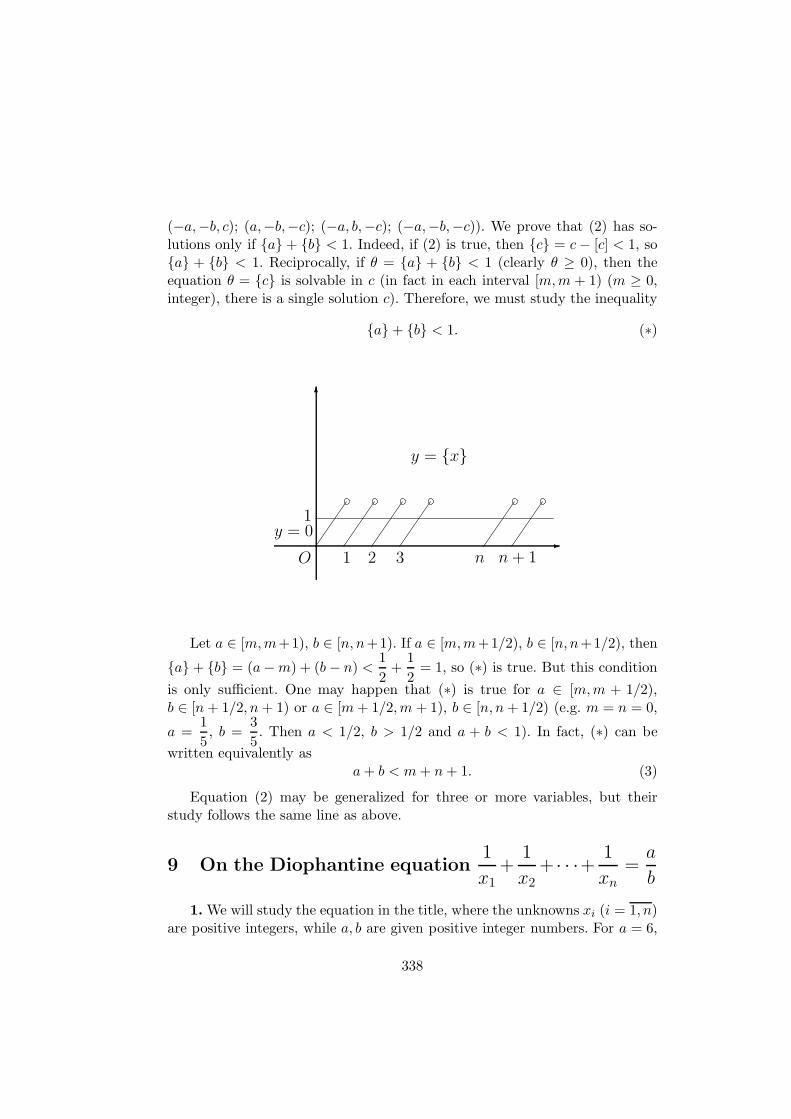
(−a,−b, c); (a,−b,−c); (−a, b,−c); (−a,−b,−c)). We prove that (2) has so-lutions only if a + b < 1. Indeed, if (2) is true, then c = c− [c] < 1, soa + b < 1. Reciprocally, if θ = a + b < 1 (clearly θ ≥ 0), then theequation θ = c is solvable in c (in fact in each interval [m,m + 1) (m ≥ 0,integer), there is a single solution c). Therefore, we must study the inequality

a + b < 1. (∗)

6

-

1y = 0

O 1 2 3 n n + 1

y = x

Let a ∈ [m,m+1), b ∈ [n, n+1). If a ∈ [m,m+1/2), b ∈ [n, n+1/2), then

a + b = (a−m) + (b− n) <1

2+

1

2= 1, so (∗) is true. But this condition

is only sufficient. One may happen that (∗) is true for a ∈ [m,m + 1/2),b ∈ [n+ 1/2, n + 1) or a ∈ [m+ 1/2,m + 1), b ∈ [n, n+ 1/2) (e.g. m = n = 0,

a =1

5, b =

3

5. Then a < 1/2, b > 1/2 and a + b < 1). In fact, (∗) can be

written equivalently asa+ b < m+ n+ 1. (3)

Equation (2) may be generalized for three or more variables, but theirstudy follows the same line as above.

9 On the Diophantine equation1

x1+

1

x2+ · · ·+ 1

xn=a

b

1. We will study the equation in the title, where the unknowns xi (i = 1, n)are positive integers, while a, b are given positive integer numbers. For a = 6,

338

b = n2−1, this contains the OQ.1119 [1] (by putting x1 = y1, x2 = y1+y2, . . . ,xn = y1 + y2 + · · ·+ yn). The particular case n = 3 of this Open Problem will

be studied in detail. Clearly, for n = 1 one has x1 =b

a, which is integer only

if a|b. Let n = 2. The equation

1

x1+

1

x2=a

b(1)

has been studied in detail in [2]. See also [3]. We will show that the resolvationof the general equation reduces inductively to the resolvation of equations oftype (1).

Let n = 3. We may suppose that x1 ≤ x2 ≤ x3. Thus, if

1

x1+

1

x2+

1

x3=a

b, (2)

thena

b≤ 3

x1, implying x1 ≤ 3b

a. This means that x1 can take a finite number

of values (at most

[3b

a

]values). Let x0 be such a value. Then

1

x2+

1

x3=a

b− 1

x0=ax0 − b

bx0=A

B.

Thus1

x2+

1

x3=A

B(3)

which is an equation of type (1). Thus, in order to solve equation (2) we mustsolve a finite number of equations of type (3). For general n we can assume

x1 ≤ x2 ≤ · · · ≤ xn. Thusa

b≤ n

x1, which gives x1 ≤ nb

a, i.e. a finite number of

values. For each fixed value of x1 one obtains an equation of n− 1 unknown.

1

x2+ · · · + 1

xn=A

B, (4)

where x2 ≤ (n− 1)B

A, etc.; inductively all will be reduced to equations of type

(1).2. We will take as an example the case n = 3 of OQ.1119, i.e. the equation

1

x+

1

x+ y+

1

x+ y + z=

3

4. (5)

339

Clearly x ≥ 2; while for x ≥ 4 one has x + y ≤ 5, x + y + z ≥ 6, so the

sum of the left side is ≤ 1

4+

1

5+

1

6=

37

60. Now,

3

4≤ 37

60, i.e. 180 ≤ 148 is

impossible. Therefore, we must have x > 1, x < 4, i.e. x ∈ 2, 3.a) Let x = 2. By

3

4− 1

2=

1

4one obtains the equation

1

t+

1

t+ z=

1

4(6)

where y+ 2 = t. By elementary transformations from (6), we get the equation

t2 + t(z − 8) − 4z = 0. (7)

This gives t1,2 =8 − z ±

√z2 + 64

2, and since t > 0,

t =8 − z +

√z2 + 64

2. (8)

Here z2 + 64 = u2, n ∈ N, otherwise t is irrational. Writing 64 = (u −z)(u + z), and considering the divisors 1, 2, 4, 8, 16, 32, 64 of 64, by an easyverification follows u = 10, z = 6; respectively u = 17, z = 15. By (8) thesegive t = 6, respectively t = 5. Thus all solutions of equation (6) are:

z = 6, y = 4 and z = 15, y = 3. (9)

b) x = 3. Now, by3

4− 1

3=

5

12we get the equation

1

t+

1

t+ z=

5

13, (10)

where t = y+3. We could use the method of a) however we will follow anotherway, i.e. by solving an equation of type (see [2])

1

a+

1

b=

5

12. (11)

Since 12(a+ b) = 5ab, put (a, b) = d, i.e. a = dA, b = dB, with (A,B) = 1.Then 12(A + B) = 5dAB, and by the known fact that (AB,A + B) = 1,it follows that AB|12, i.e. AB ∈ 1, 2, 3, 4, 6, 12. But (5, 12) = 1 implies5|(A + B), so we immediately get the solutions A = 1, B = 4; A = 2, B = 3.Then d = 3 or d = 2 and we obtain a = 3 · 1 = 3, b = 3 · 4 = 12; respectivelya = 2 · 2 = 4, b = 3 · 2 = 6. From this we can deduce the single solution of(10), namely

y = 1, z = 2. (12)

By concluding, all solutions of the equation (5) are the following:

x = 2, y = 4, z = 6; x = 2, y = 3, z = 15; x = 3, y = 1, z = 2.

340

References


[2] J. Sandor, On two Diophantine equations (Hungarian), Mat. Lapok,Cluj, 8/2001, 285-286.

[3] J. Sandor, Geometric theorems, Diophantine equations and arithmeticfunctions, American Research Press, New Mexico, 2002.

10 Harmonic triangles

1. Let ABC be a triangle with side lengths a, b, c. If C = 60, problemUS4 presented to the XXth IMO asked for a proof of relation

c

a+c

b≥ 2. (1)

For (1) quite complicated proofs were given. We note here that, by usingelementary means, in fact an easier proof of a stronger relation can be deduced.Indeed, (1) can be written also as

H(a, b) ≤ c, (2)

whereH(a, b) denotes the harmonic mean of a and b. Remark that, the strongerinequality

A(a, b) =a+ b

2≤ c (3)

is valid. Indeed, a + b ≤ 2c ⇔ (a + b)2 ⇔ 4c2, or a2 + 2ab + b2 ≤ 4c2 =4(a2+b2−ab), since c2 = a2+b2−2ab cos 60 = a2+b2−ab. The last inequalitybecomes 3(a− b)2 ≥ 0, which is obvious. Therefore

H(a, b) ≤ G(a, b) ≤ A(a, b) ≤ c (4)

is valid in any triangle ABC having C = 60. Since a = 2R sinA, etc., and

sinA+ sinB = 2 sinA+B

2cos

A−B

2, sinC = 2 sin

C

2cos

C

2,

we can remark that, in any triangle ABC, relation (3) is valid iff

cosA−B

2≤ 2 sin

C

2. (5)

341

The case sinC

2=

1

2is a particular case of (5).

2. Now, let us suppose that ABC has integral sides. We say that thetriangle ABC is harmonic relatively to the vertex C, if

H(a, b) = c. (6)

We say that the triangle ABC is harmonic, if

H(a, b, c) = integer, (7)

where H(a, b, c) = 3/

(1

a+

1

b+

1

c

)denotes the harmonic mean of a, b, c. In

what follows we shall study these two types of harmonic triangles.Relation (6) can be written also as

2ab = (a+ b)c (8)

Let gcd(a, b) = d, i.e. a = da1, b = db1, with (a1, b1) = 1. Then (8) becomes2da1b1 = (a1+b1)c. This implies a1b1|(a1+b1)c, and since it is well-known thatfor (a1, b1) = 1 one has also (a1 + b1, a1b1) = 1, we get a1b1|c, so c = ka1b1.

This in turn implies 2d = k(a1 + b1), so d =k(a1 + b1)

2, where at least one of

k and a1 + b1 is an even number. From this we get

a =ka1(a1 + b1)

2, b =

kb1(a1 + b1)

2, c = ka1b1 (9)

with (a1, b1) = 1 (and at least one of k and a1 + b1 = even). Now a+ b > c, i.e.k(a1 + b1)

2(a1 + b1) > ka1b1 ⇔ (a1 + b1)

2 > 2a1b1 is always true. The other

inequalities b+ c > a and a + c > b lead to relations of type a21 + 2a1b1 > b21

and b21 + 2a1b1 > a21 so −2a1b1 < a2

1 − b21 < 2a1b1, i.e. |a21 − b21| < 2a1b1.

All in all, the triangle ABC is harmonic relatively to C, if its sides aregiven by (9), where (a1, b1) = 1; k or a1 + b1 are even; and

|a21 − b21| < 2a1b1 (∗)

For example, when a1 = b1 + 1 and k = even, the inequality (∗) is true,since 2b1 + 1 < 2b1(b1 + 1) ⇔ 1 < 2b21 ≥ 2.

3. Now, we shall determine all harmonic triangles of type 2, i.e. for which(7) is true, i.e. ∑

ab|3abc. (10)

342

Let d = gcd(a, b, c), i.e. a = da1, b = db1, c = dc1 where (a1, b1, c1) = 1.

Then∑

a1b1|3da1b1c1. Let D = gcd(∑

a1b1, a1b1c1

). Then a1b1c1 = Dk,

∑a1b1 = Dk′, where (k, k′) = 1 so Dk′|3dDk, i.e. k′|3dk. This implies k′|3d,

so∑

a1b1 = Dk′|3dD. Let 3dD = m∑

a1b1, i.e. d =m∑

a1b1

3D. This gives

a = da1 = a1

m∑

a1b1

3D, b = db1 = b1

m∑

a1b1

3D,

c = cc1 = c1m∑

a1b1

3D.

Here D|∑

a1b1, so for a, b, c to be integers, we have two possibilities:

1) 3|m. Let m = 3s. Then

a =sa1

∑a1b1

D, b =

sb1∑

a1b1

D, c =

sc1∑

a1b1

D.

Clearly a+ b > c if a1 + b1 > c1. Therefore (a1, b1, c1) = 1 must satisfy alsothe inequalities a1 + b1 > c1, b1 + c1 > a1, a1 + c1 > b1.

2) 3 ∤ m. Remark that we cannot have 3 ∤∑

a1b1, since then we must

have 3|a1, 3|b1, 3|c1, contradiction to (a1, b1, c1) = 1. Thus we have 3|∑

a1b1(and again, of course a1 + b1 > c1, etc.).

These two cases determine all harmonic triangles.

11 A Diophantine equation involving Euler’s

totient

The equation in the title is

ϕ(x1x2 . . . xn) = ϕ(x1) + ϕ(x2) + · · · + ϕ(xn). (1)

The aim of this Note is to prove that equation (1) has a finite number ofsolutions. For particular n, all solutions can be obtained by verifications. Themethod is based on two simple lemmas.

Lemma 1. For all positive integers x and y one has

ϕ(xy) ≥ ϕ(x)ϕ(y) (2)

343

with equality only when x and y are coprime.Proof. This inequality is well known, see e.g. [3]. In fact, if one denotes

by P = product of all common prime divisors of x and y, then immediatelyfollows the identity

ϕ(xy) =P

ϕ(P )ϕ(x)ϕ(y),

where P ≥ ϕ(P ). This may be proved e.g. by

ϕ(x) = x∏

q/x,prime

(1 − 1

q

).

Lemma 2. For n ≥ 2 and ui > 2 positive integers (i = 1, 2, . . . , n), onehas

u1u2 . . . un > u1 + u2 + · · · + un. (3)

Proof. For n = 2 this follows from (u1−1)(u2−1) > 1 (i.e. u1u2 > u1+u2),valid for u1 > 2, u2 > 2. Now, by admitting that (3) is true for n, by

(u1 . . . un)un+1 > (u1 + · · · + un)un+1 > u1 + · · · + un + un+1

since this is equivalent to

(u1 + · · · + un − 1)(un+1 − 1) > 1.

So, by induction, relation (3) is valid for all n ≥ 2.Now, first consider the case n = 2. By (2) and the notations ϕ(x1) = u,

ϕ(x2) = v one can write: u+ v ≥ uv, i.e. (u− 1)(v − 1) ≤ 1.We have two casesa) (u− 1)(v − 1) = 0b) (u− 1)(v − 1) = 1.In case a) we have u = 1 or v = 1. Thus ϕ(x1) = 1, i.e. x1 = 1 or x1 = 2,

in which case ϕ(x2) = 1 +ϕ(x2) (which is impossible), or ϕ(2x2) = 1 +ϕ(x2),for x2 = odd this cannot be true, since then ϕ(2x2) = ϕ(2)ϕ(x2) = ϕ(x2) 6=1 + ϕ(x2).

If x2 is even, let x2 = 2km, with m = odd. Then ϕ(2x2) = ϕ(2k+1m) =ϕ(2k+1)ϕ(m) = 2kϕ(m) = 1 + ϕ(2km), only if 2kϕ(m) = 1 + 2k−1ϕ(m), or2k−1ϕ(m) = 1. Then k = 1 and ϕ(m) = 1. Thus m = 1 or 2, and clearly wehave determined all solutions.

In case b) we have u = 2 and v = 2. Thus ϕ(x1) = 2 and ϕ(x2) = 2. Thenϕ(x1x2) = 4 etc.

344

Now, let n = 3, i.e. consider the equation ϕ(x1x2x3) = ϕ(x1) + ϕ(x2) +ϕ(x3). By (2) one has clearly ϕ(x1x2x3) ≥ ϕ(x1)ϕ(x2)ϕ(x3), and by (3) wecannot have ϕ(xi) > 2 for all i = 1, 2, 3. Let ϕ(xi) = ui. Then, let u1 ∈ 1, 2.For u1 = 1 one gets 1 + u2 + u3 ≥ u2u3, i.e. (u2 − 1)(u3 − 1) ≤ 2. Thus onehave to distinguish the cases:

a) (u2 − 1)(u3 − 1) = 1b) (u2 − 1)(u3 − 1) = 2

and in each case one arrives to a finite number of solutions, and these solutionsmay be obtained by direct verifications. For u1 = 2, one gets 2 + u2 + u3 ≥2u2u3, implying u2 +u3 ≥ 2(u2u3 − 1) > u2u3 if u2u3 > 2. Thus (u2 − 1)(u3 −1) < 1. Here it is easy to study all possibilities to deduce the finite number ofpossible solutions.

In the general case one can follow the same argument. Namely, let ϕ(xi) =ui. By the inequality ϕ(x1 . . . x2) ≥ ϕ(x1) . . . ϕ(xn) (which is a consequenceof Lemma 1 with induction), and by relation (3) one can deduce that thereexists i0 ∈ 1, . . . , n, with xi0 ∈ 1, 2. Let i0 = 1 (for simplification ofnotation), when ϕ(x1) = 1, then x1 ∈ 1, 2 and one obtains ϕ(x2 . . . xn) =1+ϕ(x2)+· · ·+ϕ(xn) or ϕ(2x2 . . . xn) = 1+ϕ(x2)+· · ·+ϕ(xn). From 1+ϕ(x2)+· · · + ϕ(xn) ≥ ϕ(x2) . . . ϕ(xn) we have that there exists j0 ∈ 2, . . . , n withϕ(xj0) ∈ 1, 2, 3. (Since we can prove, completely analogously with Lemma2, that for ui > 3, 1+u2 + · · ·+un < u2 . . . un for n ≥ 2). When ϕ(x1) = 2, wehave 2+ϕ(x2)+ · · ·+ϕ(xn) ≥ 2ϕ(x2) . . . ϕ(xn), implying ϕ(x2)+ · · ·+ϕ(xn) ≥2[ϕ(x2)+ · · ·+ϕ(xn)−1] > ϕ(x2) . . . ϕ(xn), if ϕ(x2) . . . ϕ(xn) > 2. By Lemma2, this is impossible if all ϕ(xi) > 2 for i ∈ 2, . . . , n. Thus there existsi1 ∈ 2, . . . , n with ϕ(xi1) ∈ 1, 2. In all cases, we obtain an equation withn− 1 arguments, then two (or three) equations with n− 2 arguments, and soon. Since the equation ϕ(x) = k can have only a finite number of solutions(since, e.g. for x > 6, by the known inequality ϕ(x) >

√x it follows x < k2),

finally all equations can have a finite number of solutions. Indeed, one canprove:

Theorem. The equation (1) has at most a finite number of solutions.Proof. By (2), equation (1) implies

u1 + u2 + · · · + un ≥ u1u2 . . . un (4)

where ui ≥ 1 (i = 1, 2, . . . , n) are positive integers, ui = ϕ(xi).First we prove that inequality (4) has a finite number of solutions

(u1, . . . , un). Let u1 ≤ u2 ≤ · · · ≤ un. Then (4) yields u1u2 . . . un ≤ nun

or u1u2 . . . un−1 ≤ n. Thus 1 ≤ u1 ≤ u2 ≤ · · · ≤ un−1 ≤ n, which means thatthe numbers u1, . . . , un−1 can take at most the values 1, 2, . . . , n. For un we

345

have un(u1u2 . . . un−1 − 1) ≤ u1 + u2 + · · ·+ un−1, i.e. un ≤ u1 + · · · + un−1

u1u2 . . . un−1 − 1,

if u1u2 . . . un−1 > 1 (if not, then u1 = · · · = un−1 = 1, and we obtain theequation ϕ(x1 . . . xn) = n− 1+ϕ(xn) which we study separately. Thus un cantake a finite number of values, too. Since the equation ϕ(x) = k (k fixed) canhave at most a finite number of solutions, the proof (in this case) is completed.

For the equation ϕ(x1 . . . xn) = n−1+ϕ(xn) we note that by ϕ(x1 . . . xn) ≥ϕ(x1 . . . xn−1)ϕ(xn) we can deduce ϕ(xn)[ϕ(x1 . . . xn−1) − 1] ≤ n − 1 thus, ifϕ(x1 . . . xn−1) 6= 1, ϕ(xn) ≤ n − 1. If ϕ(x1 . . . xn−1) = 1, then x1 . . . xn−1 ∈1, 2, and the proof is finished. For Diophantine equations involving variousarithmetical functions we quote [1], [2].

References

[1] C.A. Nicol, Some Diophantine equations involving arithmetic functions,J. Math. Anal. Appl., 15(1966), 154-161.

[2] J. Sandor, Some Diophantine equations for particular arithmetic func-tions, Seminarul de teoria structurilor, no.53, Univ. Timisoara, Romania,1989, 1-10.

[3] J. Sandor, Some arithmetic inequalities, Bulletin Number Theory Rel.Topics, 11(1987), 149-161.

12 On f(n) + f(n + 1) + · · · + f(n + k) = f(n)f(n + k)

for f ∈ ϕ, ψ, σOur aim is to study the equations in the title in positive integers n, and

particular values of k for the arithmetical functions ϕ (Euler’s totient), ψ(Dedekind’s function) and σ (sum of divisors).

Theorem 1. The only solution in positive integers of the equation

ϕ(n) + ϕ(n+ 1) + ϕ(n + 2) = ϕ(n)ϕ(n + 2) (1)

is n = 3.Proof. An easy computation shows that for n < 19, the only solution of

(1) is n = 3: ϕ(3) + ϕ(4) + ϕ(5) = ϕ(3)ϕ(5), i.e. 2 + 2 + 4 = 2 · 4. Let nown ≥ 19. We note that for such n one has

ϕ(n) >√n+ 2. (2)

346

This can be proved by many arguments. For example, in [2] it is provedthat

ϕ(n) > 6n/(12 + 5 log n).

Now, the inequality 6n/(12 + 5 log n) >√n+ 2 becomes

6√n >

(1 +

2√n

)(12 + 5 log n) = 12 +

24√n

+ 5 log n+10 log n√

n

and this is true for n ≥ 19. Here one has√n > log n for n ≥ 4, but we need a

slightly stronger 6√n > 15 log n (n ≥ 11), and since 12+

24√n< 12+

24

3= 20,

the above inequality follows. This proves (2).Now, (1) can be written as

[ϕ(n) − 1][ϕ(n + 2) − 1] = ϕ(n + 1) + 1. (3)

On the right side of (3) one has ϕ(n+ 1) + 1 ≤ n+ 1, but on the left side,for n ≥ 19 one can write that

[ϕ(n) − 1][ϕ(n + 2) − 1] > (√n+ 1)(

√n+ 2 + 1)

=√n(n+ 2) +

√n+

√n+ 2 + 1 > n+ 1,

i.e.n2 + 2n+ 1 + a > n2 + 2n+ 1 for a > 0.

This finishes the proof of Theorem 1.Theorem 2. None of the equations

ψ(n) + ψ(n + 1) + ψ(n+ 2) = ψ(n)ψ(n + 2) (2)

andσ(n) + σ(n+ 1) + σ(n + 2) = σ(n)σ(n + 2) (3)

has solutions in positive integers.Proof. Write (2) in the form

[ψ(n) − 1][ψ(n + 2) − 1] = ψ(n+ 1) + 1. (4)

Since ψ(n) ≥ n+ 1, n ≥ 2, and ψ(k) ≤ σ(k) ≤ 1 + 2 + · · · + k =k(k + 1)

2(see e.g. [3]) on the left side of (4) we have ≥ n(n+ 2), while on the right sideof (4) one has

ψ(n + 1) + 1 ≤ (n+ 1)(n + 2)

2+ 1.

347

Therefore, if (4) is true, then

n(n+ 2) − 1 ≤ (n+ 1)(n + 2)

2, (5)

i.e. n2 + n ≤ 4. Since for n ≥ 2, n(n + 1) ≥ 6, this is impossible. For n = 1,(4) doesn’t give a solution. The proof of (3) runs on the same lines.

Remark 1. The proof shows that for any arithmetical function f suchthat

f(1) = 1, f(n) ≥ n+ 1, f(n) ≤ n(n+ 1)

2, n ≥ 2

the equation

f(n) + f(n+ 1) + f(n+ 2) = f(n)f(n+ 2)

doesn’t have a solution in positive integers.Remark 2. Equations (1) and (2) are particular cases of OQ.753 and

OQ.754 (t = 1, k = 2) see [1].Theorem 3. The equations

ψ(n) + ψ(n + 1) + ψ(n+ 2) + ψ(n + 3) = ψ(n)ψ(n + 3) (6)

and

σ(n) + σ(n+ 1) + σ(n+ 2) + σ(n + 3) = σ(n)σ(n+ 3) (7)

do not have solutions in positive integers.Proof. Now the method of proof of Theorem 2 doesn’t work. We need the

following auxiliary results:

ψ(n) ≤ σ(n) < 2n log n for n ≥ 3. (8)

The result is well-known, but we give here the simple proof:

σ(n) = n∑

d|n

1

d≤ n

∑

d≤n

1

s< 2n log n,

since it is well-known that

1 +1

2+ · · · + 1

n< 2 log n for n ≥ 3.

Now, (6) can be written equivalently as:

[ψ(n) − 1][ψ(n + 3) − 1] = ψ(n + 1) + ψ(n+ 2) + 1. (8)

348

The left side of (8) is ≥ n(n + 3) for n ≥ 2, but the right side is <2(n+ 1) log(n+ 1) + 2(n+ 2) log(n+ 2) + 1, so we must have

n+ 3 < 2

(1 +

1

n

)log(n+ 1) +

(1 +

2

n

)log(n+ 2) +

1

n.

Since

1 +1

n≤ 1 +

1

3=

4

3, 1 +

2

n≤ 1 +

2

3=

5

3

we must have

3n+ 8 ≤ 6 log(n+ 2). (9)

By considering the application f(x) = 6 log(x+2)−3x−8 it is easy to seethat (9) is impossible. Clearly, for equation (7) the same argument applies.

Theorem 4. For fixed k ≥ 2 and t ≥ 1, the equations

ψt(n) + ψt(n+ 1) + · · · + ψt(n+ k) = ψt(n)ψt(n+ k) (10)

σt(n) + σt(n+ 1) + · · · + σt(n+ k) = σt(n)σt(n+ k) (11)

can have at most a finite number of solutions.Proof. The same argument as in the proof of Theorem 3 can be used.

Indeed, the left side of (10) is ≥ [(n+ 1)t − 1][(n+ k)t − 1] while the right sideis < 2t[(n + 1)t + · · · + (n+ k − 1)t] logt(n+ k − 1) or

((n + 1)t − 1)((n + k)t − 1)

n2t<k2t(n+ k − 1)t logt(n+ k − 1)

n2t.

Now, if k, t are fixed and n→ ∞ this would give 1 ≤ 0, which is impossible.Therefore n ≤ n0(k, t).

References


[2] J. Sandor, On certain Diophantine equations for particular arithmeticfunctions (Romanian), Seminarul de teoria structurilor, no.53, 1989,Univ. of Timisoara.

[3] J. Sandor, On Dedekind’s arithmetical function, Seminarul de teoriastructurilor, no.51, 1988, Univ. of Timisoara, 1-15.

349

13 On certain equations for the Euler, Dedekind,and Smarandache functions

Here appear equations of type:

f(n)f(n+ 1) . . . f(n+ k) = (f(n))t + (f(n+ k))t (1)

with f ∈ ϕ,ψ, S, where ϕ,ψ, S are the Euler totient, Dedekind’s functionsand Smarandache function, respectively.

Let f be arbitrary and suppose f(n) ≥ 2, f(n + 1) ≥ 2. Then (1) cannothave solutions for t = 1 since

f(n)f(n+ 1) . . . f(n+ k) ≥ 2f(n)f(n+ k) > f(n) + f(n+ k).

Indeed,(f(n) − 1)(f(n + k) − 1) ≥ 0 ⇒

f(n)f(n+ k) ≥ f(n) + f(n+ k) − 1 ⇒2f(n)f(n+ k) ≥ 2f(n) + 2f(n+ k) − 2 > f(n) + f(n+ k)

since f(n) + f(n+ k) ≥ 3, by assumption. It is easy to see that for n ≥ 3 onehas

ϕ(n) ≥ 2, ϕ(n + 1) ≥ 2, ψ(n) ≥ 2, ψ(n + 1) ≥ 2, S(n) ≥ 2, S(n+ 1) ≥ 2,

so only the cases n ∈ 1, 2 should be considered. Since (1) implies f(n +k)|f(n) (for t = 1) and ϕ(1) = ϕ(2) = 1; ψ(1) = 1, ψ(2) = 3, S(1) = 1,S(2) = 2 we should have

ϕ(1 + k) = 1, ϕ(2 + k) = 1, ψ(1 + k) = 1,

ψ(2 + k) = 1, ψ(2 + k) = 3, S(1 + k) = 1, S(2 + k) = 2.

Only for ϕ the k = 1 case is acceptable, but then ϕ(1)ϕ(2) = 1 6= ϕ(1) +ϕ(2). Therefore, for t = 1 the proposed equations does not have solutions.

14 Some equations involving the arithmetical

functions ϕ, σ, ψ

We will consider the following equations:

1)∑

d|nϕ(dn) =

∑

d|nϕ(nd)

350

2)∑

d|n,d6=n

(σ(d))d =∑

d|n,d6=n

(σ(d))n−d

3)∑

d|n,d6=n

ψ(d) =∑

d|n,d6=n

ψ(n− d).

In what follows all equations (1)-(3) will be solved.1) Let d1 = 1 < d2 < · · · < dr = n be all divisors of n. Then

ϕ(1n) + ϕ(dn2 ) + · · · + ϕ(dn

r ) = ϕ(nd1) + · · · + ϕ(ndr ) (1)

is impossible for n ≥ 3, since it is well known that for x ≥ 3, ϕ(x) is an evennumber. Now di ≥ 1, i = 1, r, and on the right side of (1) one has an evennumber. On the other hand, the left side of (1) is odd, since dn

2 ≥ 2n ≥ 8, soϕ(dn

2 ), . . . , ϕ(dnr ) all are even, while ϕ(1n) = 1 is odd. For n = 1 or n = 2, by

ϕ(12)+ϕ(22) = ϕ(21)+ϕ(22) one has equality, by ϕ(2) = 1. Thus all solutionsof equation 1) are n = 1 and n = 2.

2) Let d be a divisor of n. Then n = kd, so n− d = (k − 1)d ≥ d if k ≥ 2.This is true, if n ≥ 2, d 6= n. For such d’s one has (σ(d))n−d ≥ (σ(d))d. Onthe other hand, if n ≥ 3, there is at least a divisor d such that n − d ≥ 2d(since n ≥ 3d, i.e. k ≥ 3 e.g. take d = 1, when n ≥ 3 = 1 · 3). Then clearly∑

(σ(d))n−d >∑

(σ(d))d in such a case. For n = 1, 2 there is no solution,too.

3) We shall use the following property of the function ψ (see e.g. [1]):

ψ(ab) ≥ aψ(b), (∀) a, b ≥ 1. (2)

Now, if n = dk, then n− d = d(k − 1), so ψ(n − d) ≥ (k − 1)ψ(d) > ψ(d),if k − 1 > 1 for at least a divisor d. Clearly, for n ≥ 3 one has such a divisor,namely d = 1. Thus the equality

ψ(d1) + · · · + ψ(dr) = ψ(n − d1) + · · · + ψ(n − dr) (3)

cannot be true. Clearly n ≥ 2, and we do not have solutions.

References

[1] J. Sandor, On Dedekind’s arithmetical function, Seminarul de teoriastructurilor, no.51, 1988, Univ. of Timisoara, 1-15.

15 Equations with composite functions

Let d(n), σ(n), ϕ(n) denote the number of divisors, the sum of divisors, andEuler’s totient, respectively. Our aim is to solve completely the four equationsstated in the title.

351

The following well-known inequalities will be used (see e.g. [3]):Lemma 1. d(n) < 2

√n for all n ≥ 1. (1)

Lemma 2. ϕ(n) ≤ n− 1 for all n ≥ 2. (2)

Lemma 3.σ(n)

d(n)≤ n+ 1

2. (3)

Lemma 4. σ(n) < n√n for all n ≥ 2. (4)

Theorem 1. All solutions of equation σ(d(n)) = n are n = 1, 3, 4, 12. Infact, σ(d(n)) < n for all n > 12. (5)

Proof. By (3),

σ(d(n)) ≤ d(d(n))d(n) + 1

2< 2√d(n)

2√n+ 1

2

< 2

√2√n · 2

√n+ 1

2=

√2 · 4

√n(2

√n+ 1) < n ⇔

√2(2

√n+ 1) < n3/4.

Put√n = x. Then

√2(2x + 1) < x3/2 ⇔ 2(2x + 1)2 < x3 ⇔ x3 >

8x2 + 8x + 2. Let f(x) = x3 − 8x2 − 8x − 2. Since f ′(x) = 3x2 − 16x − 8,f ′′(x) = 6x− 16, clearly for all x ≥ 9 we have f ′′(x) > 0 so f ′(x) > f ′(9) > 0,f(x) ≥ f(9) = 7 > 0. Thus for n ≥ 81, the inequality σ(d(n)) < n is proved.A computer search shows that this is true for all n > 12. For n = 1, 3, 4, 12there is equality, finishing the proof of Theorem 1.

Remark. For Theorem 1 see also [2].Theorem 2. All solutions of equation d(σ(n)) = n are n = 1, 2, 3. In fact,

d(σ(n)) < n for all n ≥ 4. (6)Proof. By (1) and (4), d(σ(n)) < 2

√σ(n) < 2

√n√n = 2n3/4 < n ⇔

16n3 < n4 ⇔ n > 16. For n ≥ 4, n ≤ 16 a direct computation applies. It isimmediate that n = 1, 2, 3 are solutions.

Theorem 3. The single solution of ϕ(d(n)) = n is n = 1. In fact, for anyn ≥ 2 one has ϕ(d(n)) < n. (7)

Proof. By (2) and (1) one can write successively for n ≥ 2, ϕ(d(n)) ≤d(n)− 1 < 2

√n− 1 < n since

√n <

n+ 1

2(i.e. (

√n− 1)2 > 0). Clearly n = 1

is the single solution.Theorem 4. The single solution of equation d(ϕ(n)) = n is n = 1. In

fact, for all n ≥ 2 one has d(ϕ(n)) < n. (8)Proof. Let n ≥ 2. Then by (1) and (2) one can write d(ϕ(n)) < 2

√ϕ(n) <

2√n ≤ n ⇔ n ≥ 4. For n = 2, 3 one has ϕ(2) = 1, ϕ(3) = 2, d(1) = 1 < 2,

d(2) = 2 < 3.Remark. For difficulties regarding the equations σ(ϕ(n)) = n and

ϕ(σ(n)) = n, see [1], [4].

352

References

[1] R. K. Guy, Unsolved problems in number theory, Third Edition, 2004,Springer Verlag.

[2] J. Sandor, On a note by Amarnath Murthy, Octogon Math. Mag.9(2001), no. 2, 836-838.

[3] J. Sandor, Geometric theorems, Diophantine equations, and arithmeticfunctions, American Research Press, Rehoboth, 2002.

[4] J. Sandor, Handbook of number theory, II, Kluwer Acad. Publ., to appear.

16 On d(n) + σ(n) = 2n

In a recent paper, Jason Earls [1] raised some problems and conjec-tures on abundant and deficient numbers. Particularly, in Problem 17 hedenotes the deficiency of n by α(n) = 2n − σ(n), and notes that n =1, 3, 14, 52, 130, 184, 656, 8648, 12008, 34688, 2118656 are solutions toα(n) = d(n). Here, as usual, d(n) and σ(n) denote the number, resp., sum- ofdivisors of n. The above equation is clearly equivalent with

d(n) + σ(n) = 2n (1)

Particularly, in [1] it is asked if (1) has infinitely many solutions.Our aim in what follows is to investigate certain properties of solutions of

equation (1).Theorem 1. Let p be a prime and α ≥ 1 a positive integer. Then n = pα

is a solution to (1) only if p = 2 and α = 1 (i.e. n = 3).Proof. (1) is equivalent to

α+ 1 +pα+1 − 1

p− 1= 2pα, (2)

or after certain elementary transformations to

pα(p− 2) = p(α+ 1) − (α+ 2) (3)

For p = 2 we get α = 0; contradiction. Thus p ≥ 3. For α = 1 we get p = 3,as a solution to (3). Now, suppose p ≥ 3 and α ≥ 2. Then, by induction uponα it follows immediately that

pα > p(α+ 1) − (α+ 2), (4)

353

contradicting (3), since p − 2 ≥ 1. Indeed, for α = 2 one gets p2 > 3p − 4,i.e. p(p − 3) > −4, which is trivial. Now, assuming (4), one can write pα+1 >p[p(α+1)− (α+2)] > p(α+2)− (α+3) iff p2(α+1) > 2p(α+2)− (α+3), i.e.p[p(α+1)−2(α+2)] > −(α+3). Here p(α+1)−2(α+2) ≥ 3(α+1)−2(α+2) =α− 1 ≥ 1, and all is clear, since −(α+ 3) < 0.

Theorem 2. Let p be an odd prime. Then n = 2kp is a solution to (1)only if p = 2k+1 + 2k + 1.

Proof. Since d(n) = 2(k+1), σ(n) = (2k+1−1)(p+1), an easy computationyields that (1) is equivalent to 2k+1 +2k+2−p−1 = 0, i.e. p = 2k+1 +2k+1.

Remarks. Therefore, for primes of the form

p = 2k+1 + 2k + 1 (4)

we get a solution. For k = 1, p = 7 = prime, so n = 14. For k = 2, p = 13 =prime, so n = 52; for k = 3, p = 23 = prime, so n = 184; for k = 4, p = 41 =prime, so n = 656; for k = 7, p = 271 = prime, so n = 27 · 271 = 34688; fork = 10, p = 2069 = prime, so n = 210 · 2069 = 2118656. For k = 13 we getthe prime p = 214 + 27 = 16411, which gives the number n = 213 · 1641 =134448912, not listed by Earls.

It seems very likely that there are infinitely many primes of the form(4). If this is true, then clearly an infinite number of solutions to (1) will beprovided.

Theorem 3. Let p < q be odd primes. Then n = 2k · p · q is a solution to(1) only if

(p+ q)(2k+1 − 1) + 2k+1 + 4k + 3 = p · q (5)

There are no solutions for p = 3. The only solution for p = 5 is n =2 · 5 · 13 = 130. We cannot have k = 2. For k = 3 the only solutions arep = 19, q = 79 and p = 23, q = 47.

Proof. d(n) = 4(k + 1), σ(n) = (2k+1 − 1)(p + 1)(q + 1), and after someelementary computations, (1) can be transformed into (5). For p = 3 remark,that since 2k+1 − 1 ≥ 3, the left side of (5) becomes > 3q, while the right sideis 3q; a contradiction. For p = 5 we cannot have k ≥ 2, since then 2k+1−1 ≥ 7,so the left side of (5) will be greater than the right side. For k = 1, howeverwe can obtain the solution q = 13, yielding n = 130. For k = 2 we get7(p + q) + 19 = pq, i.e.

(p− 7)(q − 7) = 68 (6)

Here p − 7 and q − 7 are both even, and (68) is impossible, since 68 =2 · 34, where p = 9 is not a prime. For k = 3, however we get the equation15(p + q) + 31 = pq, i.e.

(p− 15)(q − 15) = 256 (7)

354

Here p − 15, q − 15 are even, and writing 256 as 256 = 2 · 128 = 4 · 64 =8 · 32 = 16 · 16, we get the only solutions p− 15 = 4, q − 15 = 64; p− 15 = 8,q − 15 = 32; i.e. p = 19, q = 79, and p = 23, q = 47 (p− 15 = 2, q − 15 = 128do not give solution, since q = 128 + 15 = 143 = 11 · 13 is not prime).

Remarks. Thus for k = 3 the only solutions are n = 23 · 23 · 47 = 8648and n = 23 · 19 · 79 = 12008, which are listed by J. Earls in [1]. Relation (5)can be written also as

(p− 2k+1 + 1)(q − 2k+1 + 1) = 22k+2 − 2k+1 + 4k + 4 (8)

Thus for k = 4 one obtains:

(p − 31)(q − 31) = 1012 (9)

Since 1012 = 2 · 506 = 2 · 2 · 253, we have the only possibility p − 31 = 2,q−31 = 506, which do not give a solution, since p = 33 is not prime! Therefore,we cannot have k = 4. Similarly for k = 5 one has

(p− 63)(q − 63) = 4056, (10)

and since 4056 = 2 · 2028 = 4 · 1014 = 8 · 507, we cannot have again solutionby p = 63 + 4 = 67, q = 63 + 1014 = 1077, which is not prime.

References


355

356

Chapter 9

Arithmetic functions

”... There still remain three studies suitable for free man. Arithmetic isone of them.”

(Plato)

”... The story was told that the young Dirichlet had as a constant com-panion all his travels, like a devout man with his prayer book, an old, worncopy of the Disquisitiones Arithmetica of Gauss.”

(H. Tietze)

357

1 The non-Lipschitz property of certain arithmeticfunctions

Let d, σ, ϕ, π be the usual arithmetic functions denoting respectively thenumber of divisors, sum of divisors, Euler’s totient and the counting functionof primes, respectively.

We note here that none of these functions has the Lipschitz property, i.e.

|f(x) − f(y)| ≤ L|x− y| (L > 0 constant), x, y ∈ N. (1)

First remark that by Dirichlet’s theorem, for all m ≥ 1 there are infinitelymany primes n of the form n = k · 2m − 1. Now

d(n + 1) − d(n) = d(k2m) − 2 ≥ d(2m) − 2 = m+ 1 − 2 = m− 1,

so for m→ ∞ we get d(n + 1) − d(n) → ∞. Therefore

lim supn→∞

[d(n + 1) − d(n)] = +∞ (2)

which means that d cannot have the Lipschitz property (1). We have used alsothe property d(ab) ≥ d(a). For the function σ remark that:

σ(n!) − σ(1)

n! − 1=σ(n!) − 1

n! − 1=σ(n!)

n!

1 − 1

σ(n!)

1 − 1

n!

,

and byσ(n!)

n!=∑

d|n!

1

d≥ 1 +

1

2+ · · · + 1

n

one hasσ(n!)

n!→ ∞, n→ ∞, giving

limn→∞

σ(n!) − σ(1)

n! − 1= +∞. (3)

This contradicts (1) for x = n!, y = 1, f = σ.For the function ϕ it is well-known that (see e.g. [1])

lim supn→∞

[ϕ(n + 1) − ϕ(n)] = +∞ (4)

so ϕ doesn’t have as well, the Lipschitz property.

358

Finally, since π(m) > m logm and π(m) < m logm−m log logm for suffi-ciently large m, one has

π(3n) − π(2n)

n>

3n log 3n− 2n log 2n+ 2n log log 2n

n→ ∞ as n→ ∞,

so

limn→∞

[π(3n) − π(2n)

3n− 2n

]= +∞. (5)

Thus π cannot have the property (1).

References

[1] J. Sandor, D.S. Mitrinovic (in coop. with B. Crstici), Handbook of numbertheory, Kluwer Acad. Publ., 1995.

2 On certain open problems considered by Murthy

In a recent note A. Murthy [1] has considered the indices

Id = Id(n) =n

d(n), IS = IS(n) =

n

S(n), Iϕ = Iϕ(n) =

n

ϕ(n),

Iσ = Iσ(n) =n

σ(n),

where d(n), S(n), ϕ(n), σ(n) are respectively the number of divisors of n, theSmarandache function, the Euler totient, and the sum of divisors of n. Heconjectures that the functions Id, IS , Iϕ, Iσ : N∗ → N∗ are all surjective func-tions. For example, in case of Iσ this means that every positive integer k isthe abundancy index of some positive integer n, i.e. there exists n ≥ 1 withσ(n)

n= k. It is well-known that the sequence

(σ(n)

n

)

n≥2

is dense in (1,∞),

so that the above question is natural even in the weaker form: is every rationalnumber k the abundancy index Iσ(n) of some integer n? We note that for afixed k, the solutions of (1) are called k-perfect numbers; the numbers n withn(σ(n)) (i.e. k ∈ N) are called multiperfect numbers. These are extremely dif-ficult problems, and only partial solutions are known, see e.g. R. Laatsch [2]for a presentation of the abundancy index. (See also the recent book by theauthor [7].)

H.J. Kanold showed first that the set of all integers n with n|σ(n) hasasymptotic density zero. For similar results on the set of integers with d(n)|n,

359

see [5]. For example, in 1985 C.A. Spiro proved that if

S(x) = cardn ≤ x : d(n)|n,

then

S(x) = (1 + θ(1))x(log x)−1/2(log log x)−1 (2)

which improves S(x)/x → 0 as x → ∞. P. Erdos [6] proved that for n 6= 3, 5one has d(n!)|n! and this yields a weaker version of (2). We now show thatMurthy’s conjecture for the surjectivity of Iϕ is not true. Thus the proposition:for all k one can find n such that

n

ϕ(n)= k (3)

is not true! Writing (3) as n = ϕ(n)k, and remarking that for n ≥ 3, ϕ(n) iseven, this equality implies that for any k, n ≥ 3 is even. When n = 1, thenclearly k = 1; for n = 2 one has k = 2. Let n = 2mN (N odd) be even. Then(3) implies

2mN = 2m−1ϕ(N)k, i.e. 2N = ϕ(N)k. (4)

If N = 1, this is possible, namely for k = 2 (i.e. n = 2m are the solutionof (3)); let N ≥ 3, and suppose k is even. Then the left side of (4) is divisibleonly by 2, but the right side by 22, a contradiction. But the real surprise isthat one can prove that all integer solutions (n, k) or (3) are given by n = 2a,a ≥ 0, n = 2a3b, a, b ≥ 1, when k ∈ 1, 2, 3. Thus

Iϕ(N∗) ∩ N∗ = 1, 2, 3. (5)

Result (5) is essentially due to W. Sierpinski [3].

For the complete solutions of ϕ(j)n |n (ϕ(j) is the j-th iteration) see M.

Hausman [4]. For example, when j = 2, all solutions are given by

n = 1, 2a, 3, 2a · 3b, 2a · 5, 2a · 7, a, b ≥ 1 (6)

so one gets easily that Iϕϕ is not surjective.We now prove that Murthy’s conjecture on the surjectivity of IS , where S

is the Smarandache function, is correct. Let k be a given positive integer, andp > k a prime. Remark that S(kp) = p, since p! = 1 · 2 · 3 . . . k . . . p is the least

factorial such that kp|p!. Now, bykp

S(kp)=kp

p= k one has

n

S(n)= k with

n = kp. The fact that Id is not surjective (e.g. 18 6∈ Id(N∗)) has been provedrecently by M. Lee, and independently, by J. Sandor (see [8]).

360

References

[1] A. Murthy, A conjecture on d(n) and the divisor function itself as divisorwith required justification, Octogon Math. Mag., 11(2003), no.2, 647-650.

[2] R. Laatsch, Measuring the abundancy of integers, Math. Mag., 59(1986),no.2, 84-92.

[3] W. Sierpinski, Elementary theory of numbers, Warsaw, 1964.

[4] M. Hausman, The solution of a special arithmetic equation, Canad.Math. Bull. 25(1982), 114-117.

[5] J. Sandor, D.S. Mitrinovic (in coop. with B. Crstici), Handbook of numbertheory, Kluwer Acad. Publ., 1996.

[6] P. Erdos, Problem 3 of M. Schweitzer Math. Competition, Mat. Lapok(Budapest), 25(1974), no.3-4(1976), 353-357.

[7] J. Sandor (in coop. with B. Crstici), Handbook of number theory, II,Springer Verlag, 2005.

[8] J. Sandor, On certain open problems considered by A. Murthy, OctogonMath. Mag., 13(2005), no.1B, 894-896.

3 On an inequality of Moree on d(n)

Let d(n) denote the number of all distinct divisors of n. Then it is easy tosee that

d(nm) ≥ maxd(n), d(m) (1)

for all n,m ∈ N. This relation has been applied by us in certain problemsrelated to a factorial of a number ([2]). Inequality (1) may be defined as follows:

d(nm) ≥ d(n) + d(m) − 1 (2)

for all m,n ∈ N. This is due to P. Moree [1]. Clearly, (2) improves (1) sinced(m) − 1 ≥ 0, d(n) − 1 ≥ 0. On the other hand, (2) may be even refined, asfor all m > 1, n > 1 one has

d(nm) > d(n) + d(m). (3)

Therefore, for such values of n,m one has in fact

d(nm) ≥ d(n) + d(m) + 1. (4)

361

Let k ≥ 0 be a nonnegative integer. Let σk(n) be the sum of kth powers ofdivisors of n, i.e.

σk =∑

d|ndk.

We shall extend Moree’s inequality as follows:

σk(mn) ≥ σk(m) + σk(n) − 1 (5)

for all m ≥ 1, n ≥ 1, k ≥ 0. We note that for k = 0 this gives relation (2).First remark that if at least one of m,n is = 1, one has equality in (5). So

we may suppose m,n > 1. Then the following stronger result will be true:

σk(mn) > σk(m) + σk(n) for all m,n > 1. (6)

If (m,n) = 1 this is trivial, since by the multiplicativity of σk one can writeσk(mn) = σk(m)σk(n). But ab > a + b for a, b ≥ 2 since (a − 1)(b − 1) > 1implies ab > a+ b. Let us suppose that (m,n) > 1; let

m =∏

px∏

qy, n =∏

px′∏rz,

where (p, q) = (p, q) = (q, r) = 1 and x, x′, y, z are positive integers (y or zmay be zero). We do not use indices for simplicity.

Now,

σk(mn) = σk

(∏px+x′

)σk

(∏qy)σk

(∏rz)

≥ σk

(∏px+x′

)(σk

(∏qy)

+ σk

(∏rz))

= σk

(∏px+x′

)σk (qy) + σk

(∏px+x′

)σk

(∏rz)

>∏

pkx′σk

(∏px)σk

(∏qy)

+∏

pkxσk

(∏px′)σk

(∏rz)

≥ σk

(∏px)σk

(∏qy)

+ σk

(∏px′)σk

(∏rz)

= σk(m) + σk(n).

We have used the fact that (6) is valid for (m,n) = 1 (in case of(∏qy,∏

rz)

= 1) and the following known fact: σk(AB) ≥ Akσk(B) for

all A,B ≥ 1, k ≥ 0 (with strict inequality for A,B > 1).Corollary. For all m,n > 1 one has

σ(mn) > σ(m) + σ(n) (7)

andd(mn) > d(m) + d(n). (8)

Proof. Select k = 1, respectively k = 0 in relation (6).

362

References

[1] P. Moree, e-mail to J. Sandor, dated 29th April 2003.

[2] J. Sandor, On values of arithmetical functions at factorials, I, Smaran-dache Notions J., 10(1999), 87-94.

4 On duals of the Smarandache simple function

1. The Smarandache simple function is defined by

Sp(n) = mink ≥ 1 : pn|k! (1)

where p is a fixed prime number. The multiplicative ”dual” of this functionhas been defined by us (see [1]) as:

Sp∗(n) = maxk ≥ 1 : k!|pn. (2)

The additive variants of these functions are

Sp(x) = mink ≥ 1 : px ≤ k! (3)

Sp∗(n) = maxk ≥ 1 : k! ≤ pn (4)

where p > 1 is a fixed real number, and x > 0 is a real number. These functionshave been studied in [1]. For example, we have proved that:

log Sp∗(x) ∼ log x as x→ ∞ (5)

and that the series ∞∑

n=1

1

n

(log log n

log Sp∗(n)

)α

(6)

is convergent for α > 1, and divergent for α ≤ 1. The additive variants of theSmarandache function S(n) have been introduced in [2], and further general-ized by C. Adiga and T. Kim [3] and C. Adiga, T. Kim, D.D. Somashekaraand A.N. Fathima [4].

2. The aim of this note is to consider the function Sp∗(n) given by (2),which (though introduced in [10] has not been studied up to now). First wenote that the following simple result is true:

Theorem 1.

Sp∗(n) =

1, if p ≥ 32, if p = 2

= L(p).

363

Proof. If p = 2, then we cannot have k ≥ 3, since then 3|k!, but 3 ∤ 2n.Clearly kmax = 2, since 2! = 2|2n for all n ≥ 1.

For p ≥ 3 remark that we cannot have k ≥ 2, since then 2|k!|pn wouldimply 2|pn, impossible since pn is odd. Therefore (7) is proved.

Remarks. Therefore, Sp∗(n) is independent of n, i.e.

Sp∗(1) = Sp∗(2) = · · · = Sp∗(n) = constant,

when p is fixed. The things are different when one considers Sp∗(n) given by(2) not only for primes p, but arbitrary positive integers a ≥ 1.

Sa∗(n) = maxk ≥ 1 : k!|an. (8)

For example,

S6∗(n) =

3, if n = 1, 24, if n ≥ 3

(9)

Indeed, remark that k!|6 and k!|36 are valid for k ≤ 3 only, while k!|63 =23 · 33 is true for k ≤ 4. Now, for k ≥ 5, k! ≡ 0 (mod 10), while clearly 6n 6≡ 0(mod 10). This proves (9). Remark also that when a is a prime-power, a = ps,then Sps∗(n) = So∗(n) = L(p) for any s, with the same proof as (7). Hence thefunction f(a) = Sa∗(n) (n = fixed) is a prime-independent function. Also, fora = odd, f(a) = 1 for any n ≥ 1 (since for k ≥ 2, k! is even). Generally, for alla, a similar situation to (9) is true; namely Sa∗(n) can take a finite number ofvalues.

Theorem 2. Let a = pα11 pα2

2 . . . pαr

r be the prime factorization of a > 1and suppose p1 < p2 < · · · < pr. Then if p 6∈ p1, . . . , pr is any prime, then

Sa∗(n) ≤ p− 1. (10)

Proof. Suppose that k = Sa∗(n) ≥ p. Then p!|k!|an implies that p!|an,so p|an, impossible by the definition of p. Clearly, this is true for any primep 6∈ p1, . . . , pr. For example, for a = 6 = 2 · 3 one can select p = 5 and (10)gives S6∗(n) ≤ 4, in concordance with (9). For a = 30 = 2 · 3 · 5 one has

S30∗(n) ≤ 6. (11)

Remark that for a = odd one can select p = 2, so Sa∗(n) ≤ 1, which bySa∗(n) ≥ 1 gives the relation Sa∗(n) = 1, i.e. f(a) = 1.

Corollary. If (a, 3) = 1, then

Sa∗(n) ≤ 2. (12)

364

For example, S10∗(n) = 2 for any n ≥ 1.3. As we have seen, the function f(a) = Sa∗(n) for any fixed n ≥ 1,

has the property that f(ps) = f(p) = L(p), for any s ≥ 1, i.e. f is prime-independent. Now, one can ask what are the functions f , if we suppose thatf is multiplicative?

Theorem 3. Let f be multiplicative, prime-independent, and f(p) = L(p)for primes p (where L is given by (7)), f(1) = 1. Then one has

f(n) =

1, if n is odd2, if n is even

(13)

Proof. Let 1 < n =∏

pα be the prime factorization of n. If n is odd,

then clearly

f(n) =∏

f(pα) =∏

f(p) =∏

L(p) = 1 for p ≥ 3.

Now, if n is even, n = 2a∏

pα, then

f(n) = f(2a)∏

f(pα) = L(2) · 1 = 2

and (13) is proved.Remark. (13) gives an example of a strongly-multiplicative function (i.e.

multiplicative and prime-independent).Now, search for additive functions, which are prime-independent (so, they

will be strongly-additive) and which satisfy (7).Theorem 4. Let g be an additive, prime independent function such that

g(p) = L(p) for primes p, and let g(1) = 0. Then

g(n) =

1, if n is an odd prime power2, if n is a power of 2ω(n), if n is odd, and ω(n) ≥ 2,ω(n) + 1, if n is even, but it has

at least an odd divisor,

(14)

where ω(n) denotes the number of distinct prime divisors of n.Proof. Assume g(ab) = g(a)+g(b) for any (a, b) = 1, g(pα) = g(p) = L(p).

Then if n = pα (p odd), g(n) = L(p) = 1 for p ≥ 3. If n = 2α, clearly g(n) = 2.

Let n =∏

pα with π(n) ≥ 2, p ≥ 3. Then

g(n) =∑

g(pα) =∑

g(p) =∑

L(p) =∑

1 = ω(n),

365

if all p is odd. If n = 2a∏

pα, then

g(n) = g(2a) +∑

g(pα) = g(2) +∑

g(p)

= L(2) +∑

L(p) = 2(ω(n) − 1) = ω(n) + 1.

Together with g(1) = 0, (14) gives an example for a strongly-additivefunction.

References

[1] J. Sandor, On additive analogues of certain arithmetic functions, Sma-randache Notions J., 14(2004), 128-133.

[2] J. Sandor, On an additive analogues of the function S, Notes NumberTheory Discr. Math., 7(2001), 91-95.

[3] C. Adiga, T. Kim, On a generalization of Sandor’s function, Proc. Jang-jeon Math. Soc., 5(2002), 121-124.

[4] C. Adiga, T. Kim, D.D. Somashekara, A.N. Fathima, On a q-analogueof Sandor’s functions, JIPAM, 4(2003), no.5, article 84.

5 A modification of the Smarandache function

1. For a given function f : N∗ → N∗ and a given set A ⊂ N∗, in papers [1],[2] we have introduced the arithmetical function

FAf (n) = mink ∈ A : n|f(k) (1)

if this is well defined. We have also considered the ”dual” function

GAg (n) = maxk ∈ A : f(k)|n, (2)

if this is again, well defined. In various papers (see [3] and [4]), which havebeen recently published, or are under publication, we have studied certainproperties of these functions for A = N∗ and

f(k) = g(k) = k!, f(k) = g(k) = ϕ(k),

f(k) = g(k) = σ(k), f(k) = d(k),

f(k) = g(k) = S(k), f(k) = g(k) = T (k),

366

etc., where ϕ, σ, d, S, T represents Euler’s totient, the sum of divisors, numberof divisors, Smarandache’s function, and the product of divisors functions,respectively. For additive analogs, see e.g. [5], [6], [7].

2. The aim of this note is the introductions and preliminary study of aparticular case of (1) when A = N∗ and

f(k) = k! + (k − 1)! = (k − 1)!(k + 1).

Here 0! = 1. Let us denote this function by

F (n) = mink ≥ 1 : n|(k − 1)!(k + 1). (3)

This seems to be closely analogous to the Smarandache function

S(n) = mink ≥ 1 : n|k!, (4)

and we shall call it as ”a modification of the Smarandache function”.3. In spite of the similarity between (3) and (4), the two functions S(n)

and F (n) have quite distinct properties. For example, it is well-known, that

S(p) = p for all primes p. (5)

For the function F (p) we have:Theorem 1.

F (p) = p− 1 for all primes p. (6)

Proof. Clearly, p|(p − 2)!p for all primes p, so F (p) ≤ p− 1. Incidentally,for general n ≥ 2 we have n|(n− 2)!n, so by (3) we have:

F (n) ≤ n− 1 for all n ≥ 2. (7)

On the other hand, if k ≤ p−2, then p ∤ (k−1)!(k+1), since k−1 ≤ p−3and k + 1 ≤ p − 1, so the prime factors of (k − 1)! and k + 1 are less than p.This proves relation (6). It is well-known and obvious that:

S(k!) = k, for all k. (8)

Theorem 2.

F (k!) = k + 1 for all k ≥ 3, F (1!) = F (2!) = 1. (9)

367

Proof. Clearly F (1) = F (2) = 1 since 1|0! · 2, 2|0! · 2, where 0! = 1 by theknown convention. Let now k ≥ 3. Clearly k!|k!(k + 2), so F (k!) ≤ k + 1. Letus suppose that there is an m ≤ k with k!|(m − 1)!(m + 1). Since m ≤ k, som − 1 ≤ k − 1, thus (k − 1)! = (n − 1)!l, l ≥ 1, and on the other hand, onehas (m− 1)!|(m+ 1) = k!A. Since k! = (k − 1)k, one gets m+ 1 = klA. Thusm+1 ≥ k and by m+1 ≤ k+1, we can have only m+1 = k or m+1 = k+1.Since (k, k + 1) = 1, this last possibility cannot hold. But for m + 1 = k weget l = A = 1, so k− 1 = m− 1, i.e. k = m, impossible by m!|(m− 1)!(m+1).This proves relation (9).

Corollary 1. For infinitely many n one has

S(n) < F (n). (10)

Corollary 2. For infinitely many m one has

S(m) > F (m). (11)

Proof. Put n = p in (11). Then S(p) = p > p− 1 = F (p) by (5) and (6).Now, let n = k!, k ≥ 3 in (10). Then S(k!) = k < k + 1 = F (k!) by (8) and(9).

Remark. Since F (n) ≥ 1, by (7) we get the limit

limn→∞

n√F (n) = 1. (12)

References

[1] J. Sandor, On certain generalizations of the Smarandache functions,Notes Numb. Th. Discr. Math., 5(1999), no.2, 41-51.

[2] J. Sandor, On certain generalizations of the Smarandache functions,Smarandache Notions J., 11(2000), 202-212.

[3] J. Sandor, The product of divisors minimum and maximum functions,RGMIA Research Report collection, 7(2004), no.2, art.18, 11.

[4] J. Sandor, A note on the divisor minimum function, Octogon Math.Mag., 12(2004), no.1, 273-275.

[5] J. Sandor, On an additive analogue of the function S, Notes NumberTheory Discr. Math., 7(2001), 91-95.

368

[6] J. Sandor, On additive analogues of the function S, Smarandache NotionsJ., 14(2004), 128-133.

[7] J. Sandor, An additive analogue of the Euler minimum function, Adv.Stud. Contemp. Math., 10(2005), no.1, 53-62.

6 The star function of an arithmetic function

Let d(n) be the number of distinct positive divisors of n. Recently, in aninteresting note, Murthy and Bencze [1] have considered a ”star function”

d∗(n) =∑

k|nd(k),

and studied some of its properties, as well as analogous notions. We must notehere that the ”star” notation is already a standard notation when considering”unitary divisors” and associated arithmetic functions (see e.g. [2], [3]). An

integer k is called a unitary divisor of n if k|n and(k,n

k

)= 1. Then the

number of unitary divisors of n is denoted in the literature as

d∗(n) =∑

k|n,(k, n

k)=1

1.

Therefore, when using this ”star” notation, we always must note that thisis not the unitary divisor theory notation.

The star function of an arbitrary function f : N → R can be definedsimilarly as

f∗(n) =∑

k|nf(k).

Thus we get:Theorem 1. If f is multiplicative (i.e. f(mn) = f(m)f(n), for all

(m,n) = 1 and f(n) 6= 0), then f∗ is multiplicative, too, and for the primefactorization n = pα1

1 . . . pαr

r one has

f∗(n) =

r∏

i=1

(1 + f(pi) + · · · + f(pαi

i )) (1)

Particularly,

d∗(n) =∏

pα‖n

(α+ 1)(α + 2)

2=

r∏

i=1

(α1 + 1)(α1 + 2)

2. (2)

369

Proof. The first part is a classical result, see e.g. [4]. Clearly f(1) = 1.Since

d(1) + d(p) + · · · + d(pα) = 1 + 2 + · · · + (α+ 1) =(α+ 1)(α + 2)

2,

the second part also follows.Remark 1. Let ϕ be Euler’s totient. By Gauss theorem (which easily

follows from (1), too) ϕ∗(n) = n, so the star function of Euler’s totient is theidentity function. If σ denotes the sum of divisors function, then, by (1)

σ∗(n) =

r∏

i=1

[1 + (pi + 1) + · · · + (pαi

i + · · · + 1)].

This must not be confused with the sum of unitary divisors function, forwhich

σ∗(n) =r∏

i=1

(1 + pαi

i )

(see e.g. [3], [5]).Theorem 2. Let ω(n), resp. Ω(n) denote the number of distinct, respec-

tively total-number of prime factors of n. Then

3

2≤ 1

2

[1 + d(n)

1ω(n)

]≤[d∗(n)

d(n)

] 1ω(n)

≤ 1

2

[2 +

Ω(n)

ω(n)

]. (3)

Proof. By (2) one can write

d∗(n) =d(n)

2ω(n)(α1 + 2) . . . (αr + 2).

Now, by the arithmetic-geometric inequality one has

(α1 + 2) . . . (αr + 2) ≤(α1 + 2 + · · · + αr + 2

r

)r

=

(2 +

Ω(n)

ω(n)

)ω(n)

,

since ω(n) = r and Ω(n) = α1 + · · · + αr. This gives the right side of (3). Forthe second part of left side apply Chrystal’s inequality

r√

(1 + x1) . . . (1 + xr) ≥ r√x1 . . . xr + 1

with xi = αi + 1, i = 1, r. Since

d(n) = (α1 + 1) . . . (αr + 1) ≥ 2r,

370

the first inequality of (3) follows.Corollary 1. The normal order of magnitude of the arithmetical function

F =

(d∗

d

) 1ω

is3

2.

Proof. This follows by (3) and the classical result due to Hardy and Ra-

manujan that the normal order of magnitude ofΩ(n)

ω(n)is 1 (see e.g. [6]).

Theorem 3. Let d∗∗ be the star function of d∗. Then

d∗∗(n) ≤ d∗(n)d(n).

Proof. First we note the property m|n ⇒ d∗(m) ≤ d∗(n). Indeed if

n =∏

pa, m =∏

pb with b ≤ a, then

d∗(m) =∏ (b+ 1)(b+ 2)

2≤∏ (a+ 1)(a+ 2)

2= d∗(n).

Now, by definition,

d∗∗(n) =∑

k|nd∗(k) ≤

∑

k|nd∗(n) = d∗(n)

∑

k|n1 = d∗(n)d(n)

by the above proved property.Remark 2. The notation d∗∗(n) should not be confused with the number

of ”bi-unitary” divisors of n (see [4], [6]), with the same notation.Theorem 4. σ∗(n) ≤ σ(n)d(n).Proof. Similarly as above m|n ⇒ σ(n) ≤ σ(n), so

σ∗(n) =∑

k|nσ(k) ≤ σ(n)d(n).

References

[1] A. Murthy, M. Bencze, Extending the scope of some number theoreticfunctions, Octogon Math. Mag., 11(2003), no.1, 110-113.

[2] E. Cohen, The number of unitary divisors of an integer, Amer. Math.Monthly, 67(1960), 879-880.

371

[3] E. Cohen, Arithmetical functions associated with the unitary divisors ofan integer, Math. Z., 74(1960), 66-80.

[4] J.M. DeKoninck, A. Ivic, Topics in arithmetical functions, North HollandMath. Studies, 72(1980).

[5] J. Sandor, L. Toth, On certain number-theoretic inequalities, Fib. Quart.,28(1990), 255-258.

[6] J. Sandor, D.S. Mitrinovic, Handbook of number theory, Kluwer Acad.Publ., 1995.

[7] J. Sandor, On the arithmetical functions dk(n) and d∗k(n), PortugaliaeMath., 53(1996), 107-115.

7 On Jordan’s arithmetical function

Prelimiaries

Jordan’s arithmetical function is a generalization of Euler’s totient func-

tion ϕ. By definition, ϕk(n) =∑

(a1,...,ak,n)=11≤a1,...,ak≤n

1 = the number of all k-tuples

(a1, . . . , ak) with all components between 1 and n such that (a1, . . . , ak, n) = 1.We note that this function has some applications in the theory of linear groups.For k = 1 we have ϕ1 = ϕ ([4]).

Furthermore, let σk(n) be the sum of kth powers of divisiors of n, i.e.

σk(n) =∑

d|ndk. For k = 1 and k = 0 we reobtain the well-known arithmetical

functions σ1(n) = σ(n), the sum of divisors of n, and σ0(n) = d(n), the numberof divisors of n.

The aim of this note is to prove some interesting relations for the abovementioned arithmetical functions. First we need some lemmas.

Lemma 1. ∑

d|nϕk(d) = nk

Proof. Let us consider the set

S = (a1, . . . , ak) : a1, . . . , ak ∈ N∗, 1 ≤ a1, . . . , ak ≤ n =⋃

d|nSd,

where(a1, . . . , ak, n) = d iff d|n.

372

From a1 = b1d, . . . , ak = bkd,(b1, . . . , bk,

n

d

)= 1 we get b1 ≤ n

d, . . . , bk ≤

n

dand so Sd has ϕk

(nd

)distinct elements, the set S trivially has a number of

nk elements, hence we obtain

∑

d|nϕk

(nd

)= nk.

Sincen

d|n iff d|n, we have the result.

Lemma 2.

ϕk(n) = nk∑

d|n

µ(d)

dk

where µ denotes the Mobius arithmetical function.Proof. Apply Lemma 1 and the Mobius inversion formula ([2], [3]).

Lemma 3. If m|n (m divides n) thenϕr(m)

mr≥ ϕr(n)

nr.

Proof. It is immediate from the definition (and Lemma 2) that ϕr(ab) ≤(ϕr(b))a, so writing n = qm, and applying this inequality the result follows.

Theorem 1.a)∑

i|nϕk(i)d

(ni

)= σk(n), n ≥ 1

b)∑

i|nϕk(i)σk

(ni

)= nkd(n), n ≥ 1.

Proof. It is easy to see that ϕk and σk, d are multiplicative functions andby a known result ([2], [3]) the left sides in a) and b) are also multiplicative.Thus it is sufficient to prove these relations for n = pa (prime powers). Howeverwe shall use another argument, which is based on Dirichlet series. Denote

D(f, s) =

∞∑

n=1

f(n)

ns

the Dirichlet series of the arithmetical function f . It is well-known that

D(f ∗ g, s) = D(f, s)D(g, s), where (f ∗ g)(n) =∑

i|nf(i)g

(ni

)is the Dirichlet

product of f and g, by supposing that the considered series are absolute con-vergent ([3]). Let Ek be the function Ek(n) = nk and U(n) ≡ 1 the identityfunction. Then evidently,

σk(n) =∑

i|nEk(i)U

(nd

).

373

Since D(Ek, s) =

∞∑

n=1

1

ns−k= ζ(s− k) (which is true for Re s > k+ 1) and

D(U, s) = ζ(s), the Riemann zeta function, hence we have

D(σk, s) = ζ(s− k)ζ(s).

For k = 0 one has D(d, s) = ζ2(s).Similarly, from Lemma 2, we obtain

D(ϕk, s) =ζ(s− k)

ζ(s).

We now consider the identity

ζ(s− k)

ζ(s)ζ2(s) = ζ(s− k)ζ(s)

or

D(ϕk, s)D(d, s) = D(σk, s),

i.e. D(ϕk ∗ d, s) = D(σk, s). But it is well-known by the uniqueness theoremof Dirichlet series ([8]) that this implies ϕk ∗ d = σk, which is exactly a). Inorder to prove the second relation, we may consider the identity

ζ(s− k)

ζ(s)ζ(s− k)ζ(s) = ζ2(s − k)

or

D(ϕk ∗ σk, s) = D(nkd, s),

yielding relation b).Next we shall prove:Theorem 2.

∞∑

n=1

ϕk(n)xn

1 − xn=

∞∑

n=1

xnnk for |x| < 1

Proof. We need the following result:

If g(n) =∑

d|nf(d), then

∞∑

n=1

g(n)xn =∞∑

i=1

f(i)xi

1 − xi,

374

if the involved series are convergent (see [5]). To prove this, let us observe that

∞∑

n=1

g(n)xn =

∞∑

n=1

∑

i|nf(i)

xn =

∞∑

i=1

∞∑

j=1

f(i)xij

=

∞∑

i=1

f(i)xi

1 − xi, for |x| < 1.

Apply now this theorem for f(i) = ϕk(i) and use Lemma 1. One obtains

∞∑

i=1

ϕk(i)xi

1 − xi=

∞∑

n=1

nkxn,

which for k = 1 gives

∞∑

i=1

ϕ(i)xi

1 − x=

∞∑

n=1

nxx =x

(1 − x)2.

By differentiation we have

∞∑

n=1

n2xn =x(1 + x)

(1 − x)3,

hence∞∑

i=1

ϕ1(x)xi

1 − xi=x(1 + x)

(1 − x)3.

Remark. The above proved identities imply the interesting relations

(x =

1

2

):

∞∑

n=1

ϕ(n)

2n − 1= 2 and

∞∑

n=1

ϕ1(n)

2n − 1= 6.

We conclude with a result on the composite function ϕ(σk(n)).Theorem 3. Let k be an odd natural number. Then we have

lim infn→∞

ϕ(σk(n))

n= 0.

Proof. Let p be a prime number of the form p ≡ −1 (mod p1 . . . ps),where pi denotes the ith prime number. (By the well-known Dirichlet theorem

375

on arithmetical progressions, there exist such primes ([2], [3]). Then σk(p) =pk + 1 ≡ 0 (mod p1 . . . ps) and Lemma 3 (r = 1) implies the inequality

ϕ(σk(p))

p≤ ϕ(p1 . . . ps)

p1 . . . ps=

s∏

i=1

(1 − 1

pi

).

This last product tends to 0 as s → ∞ (see [2], [3]), so the theorem isproved.

Remark. For k = 1 Theorem 3 gives a result of L. Alaoglu and P. Erdos[1]. See also [6], [7]. Our argument is completely different. By more complicatedargument we can prove that

lim infn→∞

ϕ((σk(n)) log log log n)/n <∞.

References

[1] L. Alaoglu, P. Erdos, A conjecture in elementary theory of numbers, Bull.Amer. Math. Soc., 50(1944), 881-882.

[2] I. Creanga si colectiv, Introducere ın teoria numerelor, Ed. Did. Ped.,Bucuresti, 1965.


[4] C. Jordan, Traite de substitutions et des equations algebriques, Paris,1957.

[5] G. Polya, G. Szego, Aufgaben und Lehrsatze aus der Analysis, SpringerVerlag, 1924.

[6] J. Sandor, On the arithmetical functions ϕk and σk, Math. Student,58(1990), 49-54.

[7] J. Sandor, On Euler’s arithmetical function, Proc. VIIth National Conf.on Algebra, Brasov, Romania, 1988.

[8] E.C. Titchmarsch, The theory of functions, Oxford Univ. Press, 2nd ed.,1978, Theorem 9.6.

376

8 Generalization of a theorem of Lucas on Euler’stotient

Let ϕ be the Euler totient function. In 1845 E. Prouchet [1] proved thatfor all m,n ≥ 1 one has

ϕ(mn) = ϕ(m)ϕ(n)d

ϕ(d), (1)

where d = (m,n) = gcd of m and n. Clearly (1) implies the multiplicativeproperty of ϕ, namely

ϕ(mn) = ϕ(m)ϕ(n) (2)

if (m,n) = 1 and reciprocally, (2) holds only if (m,n) = 1 (since (1) impliesϕ(d) = d, which is true for d = 1).

In 1891 E. Lucas [2] proved that for all m,n ≥ 1

ϕ(mn) = (m,n)ϕ([m,n]) (3)

where [m,n] = lcm of m and n.Let f : N∗ → R be an arithmetical function, such that f(n) 6= 0 for all

n ≥ 1. Then that relation

ϕ(mn) = (m,n)f(|m,n|) (4)

is satisfied by the following two functions:

f1(n) = n, n ≥ 1, f2(n) = ϕ(n).

Indeed, (4) for f2 is exactly Lucas’ theorem (4), while for f1, (4) is exactlythe known relation

mn = (m,n)[m,n], (m,n ≥ 1). (5)

In 1950 H.N. Shapiro [3], as an extension of Prouchet’s theorem (1) in-troduced the so-called over-multiplicative functions as follows: f : N∗ → R iscalled over-multiplicative, if there exists a function g : N∗ → R, g(n) 6= 0 forall n, such that

f(mn) = f(m)f(n)g(d), m, n ≥ 1 (6)

where d = (m,n).Now, we shall prove the following generalization of the Lucas theorem:

377

Theorem 1. If f is over-multiplicative, then there exists g : N∗ → R,g(n) 6= 0 for all n ≥ 1 such that

f(mn) = f(d)g(d)f [m,n], m, n ≥ 1. (7)

Proof. Let m = dm′, n = dn′, where d = (m,n), so (m′, n′) = 1. Thensince (d, dm′n′) = d, by (6) one can write

f(d2m′n′) = f(d)f(dm′n′)g(d).

But mn = d2m′n′ and [m,n] = dm′n′ by (5). Thus (7) follows.Remarks. If f is over-multiplicative and g(1) = 1, then f is multiplicative.

Indeed, letting d = 1 in (6), it follows:

f(mn) = f(m)f(m) for (m,n) = 1 (8)

i.e. f is a multiplicative function. Generally speaking, (6) implies only that fis quasi-multiplicative, i.e.

f(mn) = kf(m)f(n) for (m,n) = 1 (9)

where k = g(1).Now, relation (7) shows that for over-multiplicative functions f , (4) is true

if and only if f(d)g(d) = d, i.e.

g(n) =n

f(n), n ≥ 1. (10)

In this case, (6) becomes

f(mn) = f(m)f(n)d

f(d)(11)

generalizing Prouchet’s relation (1). If f(1) = 1, then (11) clearly impliesthat f is multiplicative, i.e. has the property (8). But not all multiplicativefunctions satisfy (11)! Indeed, letting m = n in (11) it follows

f(m2) = mf(m). (12)

For example, the σ-function (sum of divisors) is multiplicative, but doesn’tsatisfy (12). Indeed, e.g. σ(4) = 7 6= 2σ(2) = 6. By induction easily followsthat if f(1) = 1, then

f(mα) = mf(mα−1) for all m ≥ 1, α ≥ 2. (13)

378

Now, we prove that, reciprocally, if f is multiplicative and has property(13), then it has also the property (11). Even a stronger result is true:

Theorem 2. Suppose that f(1) = 1, f is multiplicative, and f(pα) =pf(pα−1) for all primes p ≥ 2, α ≥ 2. Then (11) is true.

Proof. Let m =∏

pα∏

qβ, n = pα∏

rγ be the canonical factorizations

ofm and n. Then nm =∏

pα+α′∏qβ∏

rγ , where α+α′ ≥ 2 if (m,n) 6= 1 (if

(m,n) = 1, then (11) is trivially satisfied). We have f(pα+α′) = pf(pα+α′−1) =

pα+α′−1f(p), since from f(pn) = pf(pn−1) it follows by induction that f(pn) =pn−1f(p). Similarly, for all α0 ≥ 2, β0 ≥ 1, γ0 ≥ 2, f(pα0) = pα0−1f(p),f(qβ0) = qβ0−1f(q), f(rγ0) = rγ0−1f(r). When all α, β = 1, then f(m) =∏

f(p)∏

f(q), f being multiplicative. Therefore, we may assume that all

α, β, α′, γ ≥ 2. Thenf(mn)

f(m)f(n)=

=

∏pα+α′−1

∏qβ−1

∏rγ−1

∏f(p)

∏f(q)

∏f(r)

∏pα−1

∏qβ−1

∏pα′−1

∏rγ−1

∏f(p)

∏f(q)

∏f(p)

∏f(r)

=∏ p

f(p)=

d

f(d),

as now d =∏

pminα,α′ and in case minα,α′ ≥ 2 one can again apply

f(pn) = pn−1f(p).

References

[1] E. Prouchet, Nouv. Ann. Math., 4(1845), 75-80.

[2] E. Lucas, Theorie des nombres I, Gauthier-Villars, Paris, 1891.

[3] H.N. Shapiro, On the iterates of certain class of arithmetic functions,Comm. Pure Applied Math., 3(1950), 259-272.

9 Some arithmetic inequalities connected with thedivisors of an integer

1. Let 1 = d1 < d2 < · · · < dk = n be the consecutive divisors of n > 1.

Then, since di|n we have alson

di|n, and in fact, if di < dj , then

n

di>

n

dj. For

379

example, let k = 2n (even). Then the divisors in increasing order are

1 = d1 < d2 < · · · < dm <n

dm<

n

dm−1< · · · < n

d2<

n

d1= n (1)

thusdm+1 =

n

dm, dm+2 =

n

dm−1, . . . , dk−1 =

n

d2, dk = d2n =

n

d1.

In fact, this happens when n is not a square, since it is well-known that ifn = pα1

1 . . . pαr

r is the prime factorization of n, then

k = d(n) = (1 + α1) . . . (1 + αr)

and this is even only if all αi are not even, so n is not a square. When n is asquare, i.e. n = s2, then k is odd, k = 2m+ 1, and one can write

1 = d1 < d2 < · · · < dm < s <n

dm<

n

dm−1< · · · < n

d2<

n

d1= n (2)

wheredm+1 = s, dm+2 =

n

dm, . . . , d2m =

n

d2, d2m+1 =

n

d1.

From (1) it is clear that dm ≥ m, so by dmdm+1 = n we have n ≥ m(m+1) > m2, i.e. m <

√n. Since k = 2m, one gets

k = d(n) < 2√n for n 6= square. (3)

In (2) dm+1 = s =√n ≥ n + 1, so m ≤ √

n − 1, implying k = 2m + 1 ≤2√n− 1, i.e.

k = d(n) ≤ 2√n− 1 for n = square. (4)

We note that actually from m(m + 1) ≤ n one has the slightly strongerrelation, improving (3):

k = d(n) ≤√

1 + 4n − 1

2, for n 6= square. (3′)

2. From (1) it follows that dmdm+1 = n, so one can write didi+1 < n for1 ≤ i ≤ m− 1. Therefore,

S = d1d2 + d2d3 + · · · + dm−1dm + dmdm+1 + dm+1dm+2 + · · · + dk−1dk

= n+m−1∑

i=1

(didi+1 +

n2

didi+1

).

380

Remark that i(i + 1) ≤ didi+1 < n for 1 ≤ i ≤ m− 1, so

S < n+ (m− 1)n+

m−1∑

i=1

n2

i(i+ 1)= mn+ n2

(1 − 1

n

).

Thus

S < n2 +mn− n2

m, n 6= square. (5)

Since, by (3) m2 < n, mn − n2

m< 0 relation (5) implies the weaker in-

equalityS < n2. (6)

For n = square (i.e. case (2)) a similar argument gives (6), so the p = 2case of OQ.1284 [1] is settled. The case p = 3 can be studied in a similarmanner, with the difference that e.g. in case (1).

S′ = d1d2d3 + d2d3d4 + · · · + dm−2dm−1dm + dm−1dmdm+1

+dmdm+1dm+2 + · · · + dk−2dk−1dk

=

m−2∑

i=1

(didi+1di+2 +

n3

didi+1di+2

)+

(ndm−1 +

n2

dm−1

),

since heredm−1dmdm+1 = dm−1dm

n

dm= ndm−1 ≤ n2

and

dmdm+1dm+2 = dmn

dm· n

dm−1=

n2

dm−1≤ n2.

Nowdidi+1di+2 ≤ dm−1dmdm+1 ≤ n2 for 1 ≤ i ≤ m− 2

anddidi+1di+2 ≥ i(i + 1)(i + 2).

Using1

i(i+ 1)(i + 2)=

1

2· 1

i− 1

i+ 1+

1

2· 1

i+ 2,

by addition one gets the well-known identity

m−1∑

i=1

1

i(i+ 1)(i + 2)=

1

4+

1

2m− 1

2m− 2<

1

4,

381

so

S′ < (m− 2)n2 + 2n2 + n3 · 1

4≤ n2√n+

n3

4< n3 ⇔ n2

√3 <

3

4n3,

i.e.√n <

3

4n, i.e. 3

√n > 4, which is true for all n ≥ 2, finishing the proof of

S′ < mn2 +n3

4≤ n2√n+

n3

4< n3, n 6= square (7)

which improves the case p = 3 of [1]. When n is a square, a similar studyapplies.

I think that the most general case with d1d2 . . . dp . . . can be performedin the same lines, and I so propose for the patient reader to carry out thecalculations.

We finish with the remark that the inequality d(n) ≤ 2√n sometimes is

called as Sierpinski’s inequality [2]. (3), (4), (3’) give improvements of thisrelation.

References


[2] W. Sierpinski, Elementary theory of numbers, Warsawa, 1964.

10 A new arithmetic function

1. Let n =

r∏

i=1

pai

i ≥ 2 be the prime factorization of the positive integer n

(pi primes, ai ≥ 1). Let us define

fk(n) =

r∏

i=1

(pk

i + 1

2

)ai

, k ≥ fixed. (1)

Let fk(1) = 1 by definition. This arithmetic function appears naturallyfrom a result in [10], where it is proved that

r∏

i=1

(pk

i + 1

2

)ai

≤ σk(n)

d(n)≤

n∏

i=1

pkai

i + 1

2. (2)

See also [11] for similar relations.

382

Here σk(n) and d(n) = σ0(n) stand for the sum of kth powers of divisorsof n, and the number of divisors of n, respectively. Let σ∗k(n) and d∗(n) denotethe sum of kth powers of unitary divisors of n, and the number of unitarydivisors of n, resp. (see e.g. [2], [6], [9]). Then (2) can be rewritten as

fk(n) ≤ σk(n)

d(n)≤ σ∗k(n)

d∗(n). (3)

There is equality at each side only when n is squarefree. For k = 1 we getthe arithmetical function

f(n) =

r∏

i=1

(pi + 1

2

)ai

, r ≥ 1, (4)

with f(1) = 1. Clearly fk(n) and f(n) are examples of multiplicative functions,i.e. they satisfy the functional equation g(nm) = g(n)g(m) for (n,m) = 1.

2. Results on composite functions such as σ(ϕ(n)), d(ϕ(n)), etc., whereϕ(n) is Euler’s totient, are very difficult to obtain. For example, it is con-jectured (by Makowski and Schinzel, see e.g. [12] for recent and/or relatedresults) that

σ(ϕ(n)) ≥ n/2 (5)

for all n. We now prove the following simple result:Theorem 1. For all n ≥ 1 one has

f(ϕ(n)) ≤ n/2, (6)

with equality only for n = 1, 2, 3.Proof. It is known (see [9]) that

σ∗k(n)

d∗(n)≤ nk + 1

2. (7)

Now, by (3) and (7) we obtain f(n) ≤ n+ 1

2, implying f(ϕ(n)) ≤

ϕ(n) + 1

2≤ n

2, since ϕ(n) ≤ n − 1 for all n ≥ 2. An immediate verifica-

tion shows that for n = 1, 2, 3 there is equality, and that there are no othersuch values of n.

Remarks. 1) More generally, if an arithmetic function k(n) satisfies

σ(k(n))

d(k(n))≤ n

2, n ∈ S ⊂ N,

383

then

f(k(n)) ≤ n

2for all n ∈ S.

2) Since for n even ϕ(n) ≤ n

2, by the proof of Theorem 1 one can see that

f(ϕ(n)) ≤ n+ 2

4<n

2for n = even. (8)

3. The inequality

(x+ 1

2

)a

≥ xa + 1

2a, x > 0, a ≥ 1, applied to x = pk

i ,

a = ai, after term-by-term multiplication implies

fk(n) ≥ σ∗k(n)

D∗(n), (9)

where D∗(n) = 2Ω(n), defined in analogy with d∗(n) = 2ω(n), where ω(n),Ω(n)denote the distinct, resp. total number of prime factors of n. Relation (3) and(9) give at once

ω(n) log 2 ≤ logσ∗k(n)

fk(n)≤ Ω(n) log 2. (10)

Theorem 2. The normal order of magnitude of the arithmetical function

logσ∗k(n)

fk(n)is (log 2) log log n.

Proof. This follows by the double-inequality (10) and the well-known fact,due to Hardy and Ramanujan, that the normal order of magnitude of ω(n)and Ω(n) is log log n (see e.g. [1], [3]).

Theorem 3.

lim supn→∞

log log n

log nlog

σ∗k(n)

fk(n)≥ log 2, (11)

lim supm→∞

1

log nlog

σ∗k(n)

fk(n)≤ 1. (12)

Proof. This follows by (10) and the known facts

lim supn→∞

ω(n) log log n

log n= 1, lim sup

n→∞

Ω(n) log 2

log n= 1.

Theorem 4.

∏

n≤x

σ∗k(n)

fk(n)= 2x log log x+O(x) as x→ ∞, (13)

384

∑

2≤n≤x

1

logσ∗k(n)

fk(n)

∼ 1

log 2· x

log log x, x→ ∞. (14)

Proof. The proof of (13) is based on inequalities (10) and the known factsthat (see e.g. [1], [3])

∑

n≤x

ω(n) ∼ x log log x,∑

n≤x

Ω(n) ∼ x log log x as x→ ∞,

while (14) is a consequence of (10) and

∑

2≤n≤x

1

ω(n)∼ x

log log xand

∑

2≤n≤x

1

Ω(n)∼ x

log log x, x→ ∞,

see e.g. [4].4. By (3) and (7) we can write fk(n)/nk ≤ (nk + 1)/2nk, and since for a

prime n = p we have fk(p)/pk ≤ (pk + 1)/2pk , clearly

lim supn→∞

fk(n)

nk=

1

2. (15)

On the other hand, fk(2m)/2mk = (1 + 2−k)m/2m → 0 as m→ ∞, thus

lim infn→∞

fk(n)

nk= 0. (16)

Theorem 5.

lim infn→∞

1

ω(n)log

σ∗k(n)

fk(n)= lim sup

n→∞

1

Ω(n)log

σ∗k(n)

fk(n)= log 2 (17)

Proof. Remark thatσ∗k(p)

fk(p)= 2 for a prime p, and use inequality (10).

For the function D∗(n) = 2Ω(n) remark that

lim supn→∞

log(f(n)D∗(n)/n) = +∞. (18)

Indeed, by log(f(n)D∗(n)) =r∑

i=1

ai log(pi+1) and by the known inequality

log(pi + 1) > log pi + 2/(2pi + 1) it follows

log(f(n)D∗(n)/n) >r∑

i=1

2ai/(pi + 1) >1

2

r∑

i=1

1/pi. (19)

385

If one selects for pi, i = 1, r, the sequence of consecutive primes, then asr∑

i=1

1/pi → ∞ as r → ∞, by (19) we get the weaker result (18).

Theorem 6. There exists a sequence (nk) such that

log f(nk)D∗(nk)/nk ≫ log nk. (20)

Proof. Let nk = 2k, in which case we have

f(nk)D∗(nk)/nk =

(3

2

)k (1

2

)k

2k =

(3

2

)log nk/ log 2

,

hence

log f(nk)D∗(nk)/nk = (log nk)

log 3/2

log 2≫ log nk.

Inequality (19) suggests the introduction of the arithmetic function

h(n) =

n∑

i=1

ai

pi. (21)

Theorem 7. For all n ≥ 2 one has

4

5h(n) < log f(n)D∗(n)/n < h(n). (22)

Proof. By the known inequality log(x+ 1) < log x+ 1/√x(x+ 1), we get

log f(n)D∗(n)/n <

r∑

i=1

ai/√pi(pi + 1). (23)

Since2ai

2ai + 1≥ 4

5· ai

piand

ai√pi(pi + 1)

<ai

pi, by (23) we get relation (22).

Corollary.

lim infn→∞

f(n)D∗(n)

n= 0. (24)

Proof. h(p) =1

pfor a prime p, and apply the right side of Theorem 7.

5. For the sequence (fk(n))k≥1 we have:Theorem 8. The sequence (fk(n))k≥1 is supermultiplicative; (25)

the sequence (fk(n)/nk)k≥1 is strictly decreasing. (26)

386

Proof. It is easy to prove that

xk+m + 1

xk + 1≥ xm + 1

2, x > 0, m, k ≥ 0 (27)

where the inequality is strict, when at least one of k and m is ≥ 1. Apply (27)to x = pi, in order to obtain

fk+n(n) ≥ fk(n)fm(n), k,m ≥ 1,

which shows that (fk(n))k is supermultiplicative.The algebraic inequality

xk+m + 1

xk + 1≤ xm, x > 0, m, k ≥ 0 (28)

and relation (1) give at once that

fk+m(n) ≤ nmfk(n), k,m ≥ 1. (29)

For m = 1 inequality (29) gives fk+1(n)/nk+1 ≤ fk(n)/nk, so assertion(26) is proved, too.

6. Finally, we consider certain divisibility problems. An important propertyfor multiplicative functions, which is valid for f(n), too, is the following

Theorem 9. If m|n (m divides n), then f(m) ≤ f(n). (30)Remark. The values of f(n) are not integers for all n. For example, f(2) =

3

2. If n is odd, then all prime factors of n are odd, thus n is an integer. Let

n = 29m, with (m, 2) = 1. Then by multiplicative property of f one has

f(n) =

(3

2

)9

f(m), so 2a must divide f(m). Let p1, . . . , pt, 1 ≤ t ≤ r, be all

prime factors of n which are of the form

pi = 2mi+1Mi − 1 (Mi odd, mi ≥ 0, 1 ≤ i ≤ t).

Theorem 10. If m =

r∏

i=1

pbi

i , pi odd, then the necessary and sufficient

condition for f(n) to be an integer is that

r∑

i=1

bimi ≥ a, (31)

where 2a‖n.

387

References

[1] T. Apostol, Introduction to analytic number theory, Springer Verlag,1976.

[2] E. Cohen, Arithmetical functions associated with the unitary divisors ofan integer, Math. Z., 34(1960), 66-80.

[3] G.H. Hardy, E.M. Wright, An introduction to the theory of numbers,Oxford Univ. Press, 1960.

[4] M.J. deKoninck, On a class of arithmetical functions, Duke Math. J.,39(1972), 807-818.

[5] A. Makowski, A. Schinzel, On the functions σ(n) and ϕ(n), Colloq.Math., 8(1964), 95-99.

[6] J. Morgado, On the arithmetical function σ∗k, Portugal Math., 23(1964),35-40.

[7] C. Pomerance, On the composition of the arithmetic functions σ and ϕ,Colloq. Math., 58(1989), 11-15.

[8] J. Sandor, Remarks on the functions σ(n) and ϕ(n), Babes-Bolyai Univ.Preprint Nr.7, 1989, 7-12.

[9] J. Sandor, L. Toth, On certain number-theoretic inequalities, Fib. Quart.28(1990), 255-258.

[10] J. Sandor, An application of the Jensen-Hadamard inequality, NieuwArch. Wiskunde, 8(1990), no.4, 63-66.

[11] J. Sandor, On the arithmetical functions dk(n) and d∗k(n), PortugalMath., 53(1996), no.1, 107-115.

[12] J. Sandor, Handbook of number theory, II, Springer Verlag, 2005.

11 A generalization of Ruzsa’s theorem

Recently [1] we have published a new proof of a theorem of Ruzsa, whichstates that all even numbers a and b satisfying σ(a) = 2b, σ(b) = 2a (theso-called ”lovely pairs”) are given by

a = 2k(2q+1 − 1), b = 2q(2k+1 − 1),

388

where 2k+1 − 1 and 2q+1 − 1 are both prime numbers. The aim of this note isto show, that the methods of [1] enable us to give the following generalization.

Theorem. Let f : N∗ → N∗ be a given multiplicative arithmetic functionwhich satisfies the following properties:

1) f(2k) is odd;2) f(mn) ≥ mf(n) for all m,n ≥ 1, with equality only for m = 1;3) f [f(2k)] ≥ 2k+1 for all k ≥ 1, with equality only for k ∈ A where

A ⊂ N∗. Then all even solutions of the systemf(a) = 2bf(b) = 2a

in positive integers are given by a = 2kf(2a), b = 2qf(2k), where k, q ∈ A. Ifthere is strict inequality in at least one of 2) and 3), then the system doesn’thave even solutions.

Proof. Let a = 2kA, b = 2qB, where A and B are odd numbers. Since f ismultiplicative, f(a) = f(2k)f(A), f(b) = f(2k)f(B), so f(2k)f(A) = 2q+1B,f(2q)f(B) = 2k+1A. By 1) f(2k) is odd, so f(2k) must divide B, i.e. B =f(2k)B′. Similarly, A = f(2q)A′, where A′, B′ are odd integers. These givef(A) = 2q+1B′, f(B) = 2k+1A′. By using relations 2) and 3) one can deduce:

2q+1B = f(2k)f(A) = f(2k)f [A′f(2q)] ≥ f(2k)A′f [f(2q)] ≥ f(2k)A′2q+1.

Since B = f(2k)B′, this gives B′ ≥ A′. In a completely analogous wayone can obtain A′ ≥ B′. Thus A′ = B′, so A = f(2q)S, B = f(2k)S. Now,f(A) = 2q+1S, f(B) = 2k+1S give f [f(2qS)] = 2q+1S, f [f(2k)S] = 2k+1S.But f [f(2q)S] ≥ Sf [f(2q)] ≥ S · 2q+1. Therefore, we must have equality, soS = 1 and q ∈ A. Similarly, k ∈ A, and the theorem is proved.

When f(n) = σ(n), Ruzsa’s theorem is reobtained (select A = set ofprimes). When f(n) = nσ(n), all conditions are satisfied, with strict inequalityin 3), so in this case the system is not solvable.

References

[1] J. Sandor, On Ruzsa’s lovely pairs, Octogon Math. Mag., 12(2004), no.1,287-289.

12 On the monotonicity of the sequence (σk/σ∗k)

1. Introduction

Let n > 1 be a positive integer and k ≥ 0 a nonnegative integer. A divisord of n is called a unitary divisor of n, if (d, n/d) = 1. Let σ∗(n) be the sum of

389

unitary divisors of n, i.e.

σ∗(n) =∑

d|n,(d,n/d)=1

d. (1)

Then it is well-known (see e.g. [1], [8]) that

σ∗(n) =

r∏

i=1

(pai

i + 1), (2)

where n =n∏

i=1

pai

i is the prime factorization of n > 1 (pi distinct primes, ai ≥ 1

positive integers). More generally, if σ∗k(n) is the sum of kth powers of unitarydivisors of n (i.e. (1) generalized to dk in place of d in the sum), then, similarlyto (2), one has

σ∗k(n) =

r∏

i=1

(pkai

i + 1). (3)

We note that, for k = 0 we get the number d∗(n) = σ∗0(n) of unitarydivisors of n, when (3) gives

d∗(n) = 2r = 2ω(n), (4)

where ω(n) = r denotes the number of unitary divisors of n. The similarformulae for the (classical) sum of divisors of n are the well-known (see e.g.[2], [9], [7])

σ(n) =

r∏

i=1

(pai+1i − 1)/(pi − 1), (5)

resp.

σk(n) =r∏

i=1

(pk(ai+1)i − 1)/(pk

i − 1). (6)

For k = 0, (6) provides the number d(n) of classical divisors of n:

d(n) =r∏

i=1

(ai + 1). (7)

There are many results involving inequalities on these arithmetical func-tions. See e.g. [3]-[6]. For surveys of results, see e.g. [9], [8].

390

2. Main results

Langford ([9]) proved that

σk(n) ≤ d(n)

(nk + 1

2

), (8)

while we proved ([10], [4], [5]) the stronger relation

σk(n) ≤ d(n)σ∗k(n)

2ω(n)≤ d(n)

(nk + 1

2

). (9)

The second inequality of (9) is a consequence of the elementary inequality

r∏

i=1

(xi + 1) ≤ 2r−1

(r∏

i=1

xi + 1

)

(xi ≥ 1, r ≥ 1) (10)

applied to xi = pkai

i , r = ω(n), and using relation (3).Remark that the first inequality of (9) may be written also as

σk(n)

σ∗k(n)≤ σ0(n)

σ∗0(n). (11)

Our aim is to give a generalization of (11) as follows:

Theorem. For all fixed n ≥ 1, the sequence

(σk(n)

σ∗k(n)

)

k≥0

is monotone

decreasing.Proof. We have to prove that

σk(n)

σ∗k(n)≤ σl(n)

σ∗l (n)for all k ≥ l ≥ 0. (12)

By (3) and (6),

fk(n) = σk(n)/σ∗k(n) =

r∏

i=1

(pk(ai+1)i − 1)/(pk

i − 1)(pkai

i + 1),

so to prove that fk(n) ≤ fl(n) for k ≥ l, it will be sufficient to show that

pk(a+1) − 1

(pk − 1)(pka + 1)≤ pl(a+1) − 1

(pl − 1)(pla + 1), k ≥ l ≥ 0, p ≥ 2. (13)

391

Put pk = x, pl = y, where x > y ≥ 1. After some elementary transfor-mations (which we omit here) it can be shown that (13) becomes equivalentto

xa − ya

x− y≤ (xy)a − 1

xy − 1(x > y ≥ 1). (14)

For y = 1, relation (14) is trivial, so we may suppose y ≥ 2. Now, remarkthat

xa − ya

x− y= xa−1 + xa−2y + · · · + xya−2 + ya−1 ≤ axa−1,

by y < x and a ≥ 1. On the other hand, we will prove that

(xy)a − 1

xy − 1≥ axa−1. (15)

This is equivalent to

(xy)a − 1 ≥ axay − axa−1,

or

xay(ya−1 − a) + axa−1 − 1 ≥ 0.

Here axa−1 − 1 ≥ a− 1 ≥ 0, and ya−1 − a ≥ 2a−1 − a ≥ 0 for all a ≥ 1, so theresult follows. By (15), and the above remark, inequality (14) is established.By (13), the inequality (12) follows, so the theorem is proved.

Remarks. 1) For l = 0, k ≥ 0 arbitrary, we reobtain relation (11).2) For l = 1, k ≥ 1 we get

σk(n)

σ∗k(n)≤ σ(n)

σ∗(n), (16)

which offers an improvement of (11) for k ≥ 1, since by (11) applied to k = 1,and by (16), one has

σk(n)

σ∗k(n)≤ σ(n)

σ∗(n)≤ σ0(n)

σ∗0(n)=

d(n)

d∗(n). (17)

For other improvements of the right side of (17), see [5].

References

[1] E. Cohen, Arithmetical functions associated with the unitary divisors ofan integer, Math. Z. 74(1960), 66-80.

392

[2] G. H. Hardy and E. M. Wright, An introduction to the theory of numbers,Oxford Univ. Press, 1960.

[3] J. Sandor, An application of the Jensen-Hadamard inequality, NieuwArch. Wiskunde, Serie 4, 8(1990), no. 1, 43-66.

[4] J. Sandor, On an inequality of Klamkin with arithmetical applications,Int. J. Math. Ed. Sci. Technol. 25(1994), 157-158.

[5] J. Sandor, On certain inequalities for arithmetic functions, Notes Numb.Th. Discr. Math. 1(1995), 27-32.

[6] J. Sandor, On the arithmetical functions dk(n) and d∗k(n), PortugaliaeMath. 53(1996), no. 1, 107-115.

[7] J. Sandor, Geometric theorems, diophantine equations, and arithmeticfunctions, American Research Press, Rehoboth, New Mexico, 2002.

[8] J. Sandor, Handbook of number theory II, Springer-Verlag, 2004.

[9] J. Sandor, D. S. Mitrinovic, Handbook of number theory, Kluwer Acad.Publ., 1996.

[10] J. Sandor, L. Toth, On certain number-theoretic inequalities, Fib. Quart.28(1990), no. 3, 255-258.

13 A note on exponential divisors and related

arithmetic functions

1. Introduction

Let n > 1 be a positive integer, and n = pa11 . . . par

r its prime factorization.A number d|n is called an exponential divisor (or e-divisor, for short) ofn if d = pb1

1 . . . pbr

r with bi|ai (i = 1, r). This notion has been introduced byE. G. Straus and M. V. Subbarao [1]. Let σe(n), resp. de(n) denote the sum,resp. number of e-divisors of n, and let σe(1) = de(1) = 1, by convention.A number n is called e-perfect, if σe(n) = 2n. For results and Referencesinvolving e-perfect numbers, and the arithmetical functions σe(n) and de(n),see [4]. For example, it is well-known that de(n) is multiplicative, and

de(n) = d(a1) . . . d(ar), (1)

393

where n = pa11 . . . par

r is the canonical form of n, and d(a) denotes the numberof (ordinary) divisors of a.

The e-totient function ϕe(n), introduced and studied in [4] is multiplica-tive, and one has

ϕe(n) = ϕ(a1) . . . ϕ(ar), (2)

where ϕ is the classical Euler totient function.Let σ(a) denote the sum of (ordinary) divisors of a. The product of e-

divisors of n, denoted by Te(n) has the following expression (see [9]):

Te(n) = pσ(a1)d(a2)...d(ar)1 . . . pσ(ar)d(a1)...d(ar−1)

r (3)

A number n is called multiplicatively e-perfect if Te(n) = n2. Basedon (3), in [9] we have proved that n is multiplicatively e-perfect iff n canbe written as n = pm, where σ(m) = 2m, and p is a prime. Two notionsof exponentially-harmonic numbers have been recently introduced by theauthor in [11]. Finally, we note that for a given arithmetic function f : N∗ →N∗, in [5], [6] we have introduced the minimum function of f by

Ff (n) = mink ≥ 1 : n|f(k) (4)

Various particular cases, including f(k) = ϕ(k), f(k) = σ(k), f(k) =d(k), f(k) = S(k) (Smarandache function), f(k) = T (k) (product of ordinarydivisors), have been studied recently by the present author. He also studiedthe duals of these functions (when these have sense) defined by

F ∗f (n) = maxk ≥ 1 : f(k)|n (5)

See e.g. [10] and the References therein.

2. Main notions and results

The aim of this note is to introduce certain new arithmetic functions,related to the above considered notions.

Since for the product of ordinary divisors of n one can write

T (n) = nd(n)/2, (6)

trying to obtain a similar expression for Te(n) of the product of e-divisors ofn, by (3) the following can be written:

Theorem 1.

Te(n) = (t(n))de(n)/2, (7)

394

where de(n) is the number of exponential divisors of n, given by (1); while thearithmetical function t(n) is given by t(1) = 1

t(n) = p2

σ(a1)d(a1)

1 . . . p2

σ(ar)d(ar)

r (8)

n = pa11 . . . par

r being the prime factorization of n > 1.Proof. This follows easily by relation (3), and the definition of t(n) given

by (8).Remark. For multiplicatively perfect numbers given by T (n) = n2, see

[7]. For multiplicatively deficient numbers, see [8].Remark that

de(n) ≤ d(n) (9)

for all n, with equality only for n = 1. Indeed, by d(a) < a+ 1 for a ≥ 2, via(1) this is trivial.

On the other hand, the inequality

t(n) ≤ n (10)

is not generally valid. Let e.g. n = pq11 . . . pqr

r , where all qi (i = 1, r) are primes.

Then, by (8) t(n) = pq1+11 . . . pqr+1

r = (p1 . . . pr)n > n. However, there is aparticular case, when (10) is always true, namely suppose that ω(ai) ≥ 2 forall i = 1, r (where ω(a) denotes the number of distinct prime factors of a). In

[3] it is proved that if ω(a) ≥ 2, thenσ(a)

d(a)<a

2. This gives (10) with strict

inequality, if the above conditions are valid.Without any condition one can prove:Theorem 2. For all n ≥ 1

Te(n) ≤ T (n), (11)

with equality only for n = 1 and n = prime.Proof. The inequality to be proved becomes

(p

σ(a1)/d(a1)1 . . . pσ(ar)/d(ar)

r

)d(a1)...d(ar)≤ (pa1

1 . . . par

r )(a1+1)...(ar+1)/2 (12)

We will prove that

σ(a1)

d(a1)d(a1) . . . d(ar) ≤

a1(a1 + 1) . . . (ar + 1)

2

with equality only if r = 1 and a1 = 1. Indeed, it is known that (see [2])σ(a1)

d(a1)≤ a1 + 1

2, with equality only for a1 = 1 and a1 = prime. On the

395

other hand, d(a1) . . . d(ar) ≤ a1(a2 + 1) . . . (ar + 1) is trivial by d(a1) ≤ a1,d(a2) < a2 + 1, . . . , d(ar) < ar + 1, with equality only for a1 = 1 and r = 1.Thus (12) follows, with equality for r = 1, a1 = 1, so n = p1 = prime forn > 1.

Remark. In [4] it is proved that

ϕe(n)de(n) ≥ a1 . . . ar (13)

Now, by (2), de(n) ≥ a1

ϕ(a1). . .

ar

ϕ(ar)≥ 2r if all ai (i = 1, r) are even, since

it is well-known that ϕ(a) ≤ a

2for a = even. Since d(n) = (a1+1) . . . (ar +1) ≤

2a1 . . . 2ar = 2a1+···+ar = 2Ω(n) (where Ω(n) denotes the total number of primedivisors of n), by (9) one can write:

2ω(n) ≤ de(n) ≤ 2Ω(n), (14)

if all ai are even, i.e. when n is a perfect square (right side always).Similarly, in [4] it is proved that

ϕe(n)de(n) ≥ σ(a1) . . . σ(ar) (15)

when all ai (i = 1, r) are odd. Let all ai ≥ 3 be odd. Then, since σ(ai) ≥ ai +1(with equality only if ai = prime), (15) implies

ϕe(n)de(n) ≥ d(n), (16)

which is a converse to inequality (9).

Let now introduce the arithmetical function t1(n) = p2√

a1

1 . . . p2√

ar

r ,t1(1) = 1 and let γ(n) = p1 . . . pr denote the ”core” of n (see [2]). Then:

Theorem 3.

t1(n) ≤ t(n) ≤ nγ(n) for all n ≥ 1. (17)

Proof. This follows at once by the known double-inequality

√a ≤ σ(a)

d(a)≤ a+ 1

2, (18)

with equality for a = 1 on the left side, and for a = 1 and a = prime on theright side. Therefore, in (17) one has equality when n is squarefree, while onthe right side if n is squarefree, or n = pq1

1 . . . pqr

r with all qi (i = 1, r) primes.Clearly, the functions t1(n), t(n) and γ(n) are all multiplicative.

396

Finally, we introduce the minimum exponential totient function by (4)for f(k) = ϕe(k):

Ee(n) = mink ≥ 1 : n|ϕe(k), (19)

where ϕe(k) is the e-totient function given by (2). Let

E(n) = mink ≥ 1 : n|ϕ(k) (20)

be the Euler minimum function (see [10]). The following result is true:Theorem 4.

Ee(n) = 2E(n) for n > 1. (21)

Proof. Let k = pα11 . . . pαs

s . Then k ≥ 2α1+···+αs ≥ 2s. Let s be the leastinteger with n|ϕ(s) (i.e. s = E(n) by (20)). Clearly ϕe(2

s) = ϕ(s), so k = 2s

is the least k ≥ 1 with property n|ϕe(k). This finishes the proof of (21). Forproperties of E(n), see [10].

Remark. It is interesting to note that the ”maximum e-totient”, i.e.

E∗e (n) = maxk ≥ 1 : ϕe(k)|n (22)

is not well defined. Indeed, e.g. for all primes p one has ϕe(p) = 1|n, andE∗

e (p) = +∞, so E∗e (n) given by (22) is not an arithmetic function.

References

[1] E. G. Straus and M. V. Subbarao, On exponential divisors, Duke Math.J. 41(1974), 465-471.

[2] D. S. Mitronovic and J. Sandor, Handbook of number theory, KluwerAcad. Publ., 1995.

[3] J. Sandor, On the Jensen-Hadamard inequality, Nieuw Arch Wiskunde(4)8(1990), 63-66.

[4] J. Sandor, On an exponential totient function, Studia Univ. Babes-Bolyai, Math. 41(1996), no. 3, 91-94.

[5] J. Sandor, On certain generalizations of the Smarandache functions,Notes Number Th. Discr. Math. 5(1999), no. 2, 41-51.

[6] J. Sandor, On certain generalizations of the Smarandache function,Smarandache Notion J. 11(2000), no. 1-3, 202-212.

397

[7] J. Sandor, On multiplicatively perfect numbers, J. Ineq. Pure Appl. Math.2(2001), no. 1, Article 3, 6 pp. (electronic).

[8] J. Sandor, Geometric theorems, diophantine equations, and arithmeticfunctions, American Research Press, Rehoboth, 2002.

[9] J. Sandor, On multiplicatively e-perfect numbers, to appear.

[10] J. Sandor, On the Euler minimum and maximum functions, to appear.

[11] J. Sandor, On exponentially harmonic numbers, to appear.

14 The Euler minimum and maximum functions

1. The Euler minimum function is defined by

E(n) = mink ≥ 1 : n|ϕ(k) (1)

It was introduced by P. Moree and H. Roskam [5]; and independently byJ. Sandor [7], as a particular case of the more general function

FAf (n) = mink ∈ A : n|f(k) (A ⊂ N∗), (2)

where f : N∗ → N∗ is a given function, and A is a given set of positive integers.For A = N∗, f = ϕ (Euler’s totient), one obtains the function E given by(1) (denoted also as Fϕ in [7]). Since by Dirichlet’s theorem on arithmeticalprogression, there exists a ≥ 1 such that k = an+ 1 = prime, by ϕ(k) = an:n,so E(n) is well defined.

We note that for A = N∗, f(k) = k! one reobtains the Smarandachefunction

S(n) = mink ≥ 1 : n|k!, (3)

while for A = P = 2, 3, 5, . . . = set of all primes, f(k) = k!, (2) gives a newfunction, denoted by us as P (n):

P (n) = mink ∈ P : n|k! (4)

We note that this function should not be confused with the greatest primedivisor of n (denoted also sometimes by P (n)). For properties of this function,see [6], [7].

There is a dual of (2) (see [7]), namely

GAg (n) = maxk ∈ A : g(k)|n, (5)

398

where g : N∗ → N∗, A ⊂ N∗ are given, if this is well defined. For A = N∗,g(k) = k!, this has been denoted by us by S∗(n), and called as the dual of theSmarandache function:

S∗(n) = maxk ≥ 1 : k!|n (6)

For properties of this function, see [6]. See also F. Luca [4], where a con-jecture of the author has been proved, and M. Le [3] for a recent new proof.See also K. Atanassov [1].

For A = N∗, g(k) = ϕ(k) one obtains the dual E∗(n) of the Euler minimumfunction, which we shall call as the Euler maximum function:

E∗(n) = maxk ≥ 1 : ϕ(k)|n (7)

Since for k > 6, ϕ(k) >√k, clearly k < n2, so E∗(n) ≤ n2 <∞.

Generally, for A = N∗, let us write simply FAf (n) = Ff (n), GA

g (n) = Gf (n).2. First we prove the following property of the Euler minimum function:Theorem 1. If pi (i = 1, r) are distinct primes, and αi ≥ 1 are integers,

then

maxE(pαi

i ) : i = 1, r ≤ E

(r∏

i=1

pαi

i

)≤ [E(pα1

1 ), . . . , E(pαr

r )], (8)

where [, . . . , ] denotes l.c.m.Proof. For simplicity we shall prove (8) for r = 2. Let pα, qβ be distinct

prime powers. Then E(pαqβ) = mink ≥ 1 : pαqβ|ϕ(k) = k0, so pαqβ|ϕ(k0),which is equivalent to pα|ϕ(k0), q

β|ϕ(k0), thus k0 ≥ E(pα), k0 ≥ E(qβ), im-plying E(pαqβ) ≥ maxE(pα), E(qβ). It is immediate that the same proof

applies to E(∏

pα)

≥ maxE(pα), where pα are distinct prime powers.

Therefore, the left side of (8) follows.Now, let E(pα) = k1, E(qβ) = k2, implying pα|ϕ(k1), q

β|ϕ(k2). Let[k1, k2] = g. Since k1|g, one has ϕ(k1)|ϕ(g) (by a known property of the func-tion ϕ). Similarly, since k2|g, one can write ϕ(k2)|ϕ(g). Thus pα|ϕ(k1)|ϕ(g) andqβ|ϕ(k2)|ϕ(g), yielding pαqβ|ϕ(g). By the definition (1) this gives g ≥ E(pαqβ),i.e. [E(pα), E(qβ)] ≥ E(pαqβ), so the right side of (8) for r = 2 is proved. Thegeneral case follows exactly the same lines.

Remark 1. The above proof shows that the left side of (8) holds true forany function f (for which Ff is well defined), so we get

maxFf (pαi

i ) : i = 1, r ≤ Ff

(r∏

i=1

pαi

i

)(9)

399

For the right side of (8), with the same proof the following is valid: if fhas the property

a|b ⇒ f(a)|f(b) (a, b ≥ 1), (10)

then

Ff

(r∏

i=1

pαi

i

)

≤ [Ff (pα11 ), . . . , Ff (pαr

r )] (11)

Now, if one replaces (10) with a stronger property, then a better result willbe true:

Theorem 2. Assume that f satisfies the following property

a ≤ b ⇒ f(a)|f(b) (a, b ≥ 1) (12)

Then

Ff

(r∏

i=1

pαi

i

)= maxFf (pαi

i ) : i = 1, r (13)

Proof. By taking into account of (9), one needs only to show thatthe reverse inequality is true. For simplicity, let us take again r = 2. LetFf (pα) = m, Ff (qβ) = n, with m ≤ n. Then the definition (2) of Ff im-plies that pα|f(m), qβ|f(n). By (12) one has f(m)|f(n), so pα|f(m)|f(n).We have pα|f(n), qβ|f(n), so pαqβ|f(n). But this implies n ≥ Ff (pαqβ), i.e.maxFf (pα), Ff (qβ) ≥ Ff (pαqβ). The general case follows exactly the samelines.

Remark 2. If (a, b) = 1, by writing a =

r∏

i=1

pαi

i , b =

s∏

j=1

qβj

j , (pi, qj) = 1,

it follows that

Ff (ab) = maxE(pαi

i ), E(qβj

j ) : i = 1, r, j = 1, s =

= maxmaxE(pαi

i ) : i = 1, r,maxE(qβj

j ) : j = 1, s =

= maxFf (a), Ff (b),so:

Ff (ab) = maxFf (a), Ff (b) for (a, b) = 1 (14)

When f(n) = n!, then clearly (12) is true, so (14) gives:

S(ab) = maxS(a), S(b) for (a, b) = 1, (15)

discovered by F. Smarandache [9].

400

3. The Euler minimum function must be studied essentially (by Theorem1) for prime powers pα. For values of E(p), E(p2), etc., see [5]. On the otherhand, for each prime p ≥ 3 one has

E(p − 1) = p (16)

Indeed, if (p − 1)|ϕ(k), then p − 1 ≤ ϕ(k). Since ϕ(k) ≤ k − 1 for k ≥ 3,one has p ≤ k. Now k = p gives ϕ(p) = p− 1, giving (16).

The values of the Euler maximum function E∗ given by (7) however areeven difficult to calculate in some cases. This function doesn’t seem to havebeen studied up to now.

Clearly E∗(1) = 2 since ϕ(1) = 1, ϕ(2) = 1. One has E∗(2) = 6 sinceϕ(6) = 2, 2|2, and it is well-known that ϕ(n) ≥ 4 for n ≥ 7. Now let p ≥ 3 bea prime. Since ϕ(k)|p implies ϕ(k) = 1 or ϕ(k) = p, for p ≥ 3 the last equalityis impossible for ϕ(k) is even for all k ≥ 3, we can have only ϕ(k) = 1 andkmax = 2. Actually since for k ≥ 3, ϕ(k) is even, ϕ(k)|n is impossible for n =odd, so remains k ≤ 2, and kmax = 2. We have proved:

Theorem 3. One has E∗(1) = 2, E∗(p) =

6, if p = 22, if p ≥ 3

for all primes

p; and E∗(n) = 2 for all n ≥ 1 odd. For all n ≥ 2 one has E∗(n) ≥ 2. (17)The last inequality is a consequence of ϕ(2) = 1 and the definition (7).The value 2 is taken infinitely often, but the same is true for the value 6:Theorem 4. For all α ≥ 1 one has

E∗(2 · 7α) = 6 (18)

Proof. If ϕ(k)|(2 · 7α), then assuming k ≥ 3, as ϕ(k) is even, we can onlyhave ϕ(k) = 2 or ϕ(k) = 2 · 7a where 1 ≤ a ≤ α. Now, A. Schinzel [8] hasshown that the equation ϕ(x) = 2 · 7a is not solvable for any a ≥ 1. Thus, itremains ϕ(k) = 2 and the maximal value of k ≥ 3 is k = 6. This finishes theproof of (18).

Remark. One has similarly E∗(2 · 52α) = 6 for any α ≥ 1. (19)The function E∗ can take greater values, too; the values at powers of 2 is

shown by the following theorem:Theorem 5. E∗(2m) = k, where k is the greatest number which can be

written as k = 2αp1 . . . pr, with p1 = 22α1 + 1, . . . , pr = 22αr

+ 1 distinctFermat primes, and where α = a + 1 − (2k1 + · · · + 2kr), with k1, . . . , kr ≥ 0,0 ≤ a ≤ m. (20)

Proof. Since ϕ(k)|2m, clearly ϕ(k) = 2a, where 0 ≤ a ≤ m. Nowlet k = 2αpα1

1 . . . pαr

r with p1, . . . , pr distinct odd primes. Since ϕ(k) =

401

2α−1pα1−11 . . . pαr−1

r (p1 − 1) . . . (pr − 1) = 2a, we must have α1 − 1 = · · · =αr − 1 = 0 and p1 − 1 = 2a1 , . . . , pr − 1 = 2ar with α− 1 + a1 + · · · + ar = a.This gives p1 = 2a1 + 1, . . . , pr = 2ar + 1. Since p1 is prime, it is well-knownthat it is a Fermat prime, so a1 = 2k1 , etc., and the theorem follows.

Remark 3. For m = 2 we get α ≤ 3 − (2k1 + · · · + 2kr), so with k1 = 0(when p1 = 3), we get k = 22 · 3 = 12. Another value would be k = 2 · 5 = 10,so we get

E∗(4) = 12

Similarly, for m = 3,E∗(8) = 30

If can be shown also that

E∗(16) = 60, E∗(32) = 120, E∗(64) = 240, E∗(128) = 510, etc.

However, since the structure (or the cardinality) of the Fermat primes isnot well-known, there are problems also with the calculation of great valuesof E∗(2m).

The function E∗(n) can take arbitrarily large values, since one has:Theorem 6. For all m ≥ 1 the following inequality is true:

E∗(m!) ≥ (m!)2

ϕ(m!)(21)

Proof. It is known (see e.g. [2]) that the equation

ϕ(x) = m! (22)

admits the solution x = (m!)2/ϕ(m!). Now, since ϕ(x) = m!|m!, clearlyE∗(m!) ≥ x, giving inequality (21).

Corollary. limm→∞

E∗(m!)

m!= +∞ (23)

Proof. Indeed, it is well-known (see e.g. [10]) thatm!

ϕ(m!)→ ∞ as m→ ∞.

By (21), this implies (23).

References

[1] K. T. Atanassov, Remark on Jozsef Sandor and Florian Luca’s theorem,C. R. Acad. Bulg. Sci. 55(2002), no. 10, 9-14.

[2] P. Erdos, Amer. Math. Monthly 58(1951), p. 98.

402

[3] M. Le, A conjecture concerning the Smarandache dual function, Smaran-dache Notion J. 14(2004), 153-155.

[4] F. Luca, On a divisibility property involving factorials, C. R. Acad. Bulg.Sci. 53(2000), no. 6, 35-38.

[5] P. Moree, H. Roskam, On an arithmetical function related to Euler’stotient and the discriminantor, Fib. Quart. 33(1995), 332-340.

[6] J. Sandor, On certain generalizations of the Smarandache function,Smarandache Notions J. 11(2000), no. 1-3, 202-212.

[7] J. Sandor, On certain generalizations of the Smarandache function,Notes Number Theory Discr. Math. 5(1999), no. 2, 41-51.

[8] A. Schinzel, Sur l’equation ϕ(x) = m, Elem. Math. 11(1956), 75-78.

[9] F. Smarandache, A function in the number theory, An. Univ. Timisoara,Ser. Mat., 38(1980), 79-88.

[10] J. Sandor, On values of arithmetical functions at factorials, I, Smaran-dache Notions J., 10(1999), 87-94.

15 The Smarandache minimum and maximum

functions

1. Let f : N∗ → N be a given arithmetic function and A ⊂ N a given set.The arithmetical function

FAf (n) = mink ∈ A : n|f(k) (1)

has been introduced in [4] and [5]. For A = N, f(k) = k! one obtains theSmarandache function; for A = N∗, A = P = 2, 3, 5, . . . = set of all primes,one obtains a function

P (n) = mink ∈ P : n|k! (2)

For properties of this function, see [4], [5].The ”dual” function of (1) has been defined by

GAg (n) = maxk ∈ A : g(k)|n, (3)

403

where g : N∗ → N is a given function, and A ⊂ N is a given set. Particularly,for A = N∗, g(k) = k! one obtains the dual of the Smarandache function,

S∗(n) = maxk ≥ 1 : k!|n (4)

For properties of this function, see [4], [5]. F. Luca [3], K. Atanassov [1]and L. Le [2] have proved in the affirmative a conjecture of the author.

For A = N∗ and f(k) = g(k) = ϕ(k) in (1), resp. (3) one obtains the Eulerminimum, resp. maximum-functions, defined by

E(n) = mink ≥ 1 : n|ϕ(k), (5)

E∗(n) = maxk ≥ 1 : ϕ(k)|n (6)

For properties of these functions, see [6].When A = N∗, f(k) = d(k) = number of divisors of k, one obtains the

divisor minimum function (see [4], [5], [7])

D(n) = mink ≥ 1 : n|d(k) (7)

It is interesting to note that the divisor maximum function (i.e. the ”dual”of D(n)) given by

D∗(n) = maxk ≥ 1 : d(k)|n (8)

is not well-defined! Indeed, for any prime p one has d(pn−1) = n|n and pn−1

is unbounded as p→ ∞. For a finite set A, however DA∗ (n) does exist.

On the other hand, it has been shown in [4], [5] that

Σ(n) = mink ≥ 1 : n|σ(k) (9)

(denoted there by Fσ(n)) is well defined. (Here σ(k) denotes the sum of alldivisors of k). The dual of the sum-of-divisors minimum function is

Σ∗(n) = maxk ≥ 1 : σ(k)|n (10)

Since σ(1) = 1|n and σ(k) ≥ k, clearly Σ∗(n) ≤ n, so this function iswell-defined (see [8]).

2. The Smarandache minimum function will be defined for A = N∗,f(k) = S(k) in (1). Let us denote this function by Smin:

Smin(n) = mink ≥ 1 : n|S(k) (11)

Let us assume that S(1) = 1, i.e. S(n) is defined by (1) for A = N∗,f(k) = k!:

S(n) = mink ≥ 1 : n|k! (12)

404

Otherwise (i.e. when S(1) = 0) by n|0 for all n, by (11) one gets thetrivial function Smin(n) ≡ 0. By this assumption, however, one obtains a veryinteresting (and difficult) function Smin given by (11). Since n|S(n!) = n, thisfunction is correctly defined.

The Smarandache maximum function will be defined as the dual ofSmin:

Smax(n) = maxk ≥ 1 : S(k)|n (13)

We prove that this is well-defined. Indeed, for a fixed n, there are a finitenumber of divisors of n, let i|n be one of them. The equation

S(k) = i (14)

is well-known to have a number of d(i!) − d((i − 1)!) solutions, i.e. in a finitenumber. This implies that for a given n there are at most finitely many k withS(k)|n, so the maximum in (13) is attained.

Clearly Smin(1) = 1, Smin(2) = 2, Smin(3) = 3, Smin(4) = 4, Smin(5) = 5,Smin(6) = 9, Smin(7) = 7, Smin(8) = 32, Smin(9) = 27, Smin(10) = 25,Smin(11) = 11, etc., which can be determined from a table of Smarandachenumbers:

n 1 2 3 4 5 6 7 8 9 10 11 12 13

S(n) 1 2 3 4 5 3 7 4 6 5 11 4 13

n 14 15 16 17 18 19 20 21 22 23 24 25

S(n) 7 5 6 7 6 19 5 7 11 23 4 10

We first prove that:Theorem 1. Smin(n) ≥ n for all n ≥ 1, with equality only for

n = 1, 4, p (p = prime). (15)Proof. Let n|S(k). If we would have k < n, then since S(k) ≤ k < n we

would get S(k) < n, in contradiction with n|S(k). Thus k ≥ n, and takingminimum, the inequality follows. There is equality for n = 1 and n = 4. Letnow n > 4. If n = p = prime, then p|S(p) = p, but for k < p, p ∤ S(k). Indeed,by S(k) ≤ k < p this is impossible. Reciprocally, if mink ≥ 1 : n|S(k) = n,then n|S(n), and by S(n) ≤ n this is possible only when S(n) = n, i.e. whenn = 1, 4, p (p = prime).

Theorem 2. For all n ≥ 1,

Smin(n) ≤ n! ≤ Smax(n). (16)

405

Proof. Since S(n!) = n, definition (11) gives the left side of (16), whiledefinition (13) gives the right side inequality.

Corollary. The series∑

n≥1

1

Smin(n)is divergent, while the series

∑

n≥1

1

Smax(n)is convergent.

Proof. Since∑

n≥1

1

Smax(n)≤∑

n≥1

1

n!= e − 1 by (16), this series is conver-

gent. On the other hand,∑

n≥1

1

Smin(n)≥

∑

p prime

1

Smin(p)=∑

p

1

p= +∞, so

the first series is divergent.Theorem 3. For all primes p one has

Smax(p) = p! (17)

Proof. Let S(k)|p. Then S(k) = 1 or S(k) = p. We prove that if S(k) =p, then k ≤ p!. Indeed, this follows from the definition (12), since S(k) =minm ≥ 1 : k|m! = p implies k|p!, so k ≤ p!. Therefore the greatest valueof k is k = p!, when S(k) = p|p. This proves relation (17).

Since S(p2) = 2p, for all primes p, from (11) and (13) one can deduce thefirst part of the following theorem:

Theorem 4. For all primes p,

Smin(2p) ≤ p2 ≤ Smax(2p), (18)

and more generally; for all m ≤ p,

Smin(mp) ≤ pm ≤ Smax(mp) (19)

Proof. (19) follows by the known relation S(pm) = mp if m ≤ p and thedefinitions (11), (13). Particularly, for m = 2, (19) reduces to (18). For m = p,(19) gives

Smin(p2) ≤ pp ≤ Smax(p2) (20)

The case when m is also an arbitrary prime is given inTheorem 5. For all odd primes p and q, p < q one has

Smin(pq) ≤ qp ≤ pq ≤ Smax(pq) (21)

(21) holds also when p = 2 and q ≥ 5.

406

Proof. Since S(qp) = pq and S(pq) = qp for primes p and q, the extremeinequalities of (21) follow from the definitions (11) and (13). For the inequality

qp < pq remark that this is equivalent to f(p) > f(q), where f(x) =lnx

x

(x ≥ 3). Since f ′(x) =1 − lnx

x2= 0 ⇔ x = e immediately follows that f is

strictly decreasing for x ≥ e = 2.71 . . . From the graph of this function, sinceln 2

2=

ln 4

4we get that

ln 2

2<

ln 3

3, but

ln 2

2>

ln q

qfor q ≥ 5. Therefore (21)

holds also when p = 2 and q ≥ 5. Indeed, f(q) ≤ f(5) < f(4) = f(2).Remark. For all primes p, q

Smin(pq) ≤ minpq, qp andSmax(pq) ≥ maxpq, qp. (22)

For p = q this implies relation (21).Proof. Since S(qp) = S(pq) = pq, one has

Smin(pq) ≤ pq, Smin(pq) ≤ qp, Smax(pq) ≥ pq, Smax(pq) ≥ qp.

References

[1] K. Atanassov, Remark on Jozsef Sandor and Florian Luca’s theorem, C.R. Acad. Bulg. Sci. 55(2002), no. 10, 9-14.

[2] M. Le, A conjecture concerning the Smarandache dual function, Smaran-dache Notions J. 14(2004), 153-155.



[5] J. Sandor, On certain generalizations of the Smarandache function,Smarandache Notions J., 11(2000), no. 1-3, 202-212.

[6] J. Sandor, On the Euler minimum and maximum functions,RGMIA Research Report Collection 8(1), Article 1, 2005.

[7] J. Sandor, A note on the divisor minimum function, Octogon Math.Mag., 12(2004), no.2A, 273-275.

[8] J. Sandor, The sum-of-divisors minimum and maximum functions,RGMIA Research Report Collection, 8(1), Article 20, 2005.

407

16 The pseudo-Smarandache minimum andmaximum functions

1. Introduction

K. Kashihara [2] defined the pseudo-Smarandache function Z by

Z(n) = min

m ≥ 1 : n|m(m+ 1)

2

(1)

For properties of this function see e.g. [2], [1], [6]. The dual of the pseudo-Smarandache function has been introduced and studied by the author (see [5],[6):

Z∗(n) = max

m ≥ 1 :

m(m+ 1)

2|n

(2)

More generally, for functions f, g : N∗ → N∗, the author [3], [4] (see also[6]) has defined the functions

Ff (n) = mink ≥ 1 : n|f(k), (3)

Gg(n) = maxk ≥ 1 : g(k)|n, (4)

if these functions are well-defined. Various particular cases, including f(k) =g(k) = ϕ(k), f(k) = g(k) = σ(k), f(k) = d(k), f(k) = S(k) (Smarandachefunction), f(k) = T (k) (product of ordinary divisors) have been studied bythe author. See e.g. [7] and the References therein.

The aim of this note is the initial study of the functions Z(n) and Z∗(n)given by (3), resp. (4) for the particular cases f(k) = g(k) = Z(k).

2. The pseudo-Smarandache minimum and maximum functions

The pseudo-Smarandache minimum function will be defined by

Z(n) = mink ≥ 1 : n|Z(k), (5)

while the pseudo-Smarandache maximum function will be the dual ofZ(n):

Z∗(n) = maxk ≥ 1 : Z(k)|n (6)

The particular cases of (3) and (4) for f(k) = g(k) = Z∗(k), given by (2)(i.e. the pseudo-Smarandache dual minimum and maximum functions) will bestudied in another paper.

408

Recall the following known properties of Z(n) (see e.g. [6])

Z(n) ≤

2n− 1, if n is even,n− 1, if n is odd,

(7)

Z(2k) = 2k+1 − 1, (8)

Z(p) = p− 1 for p ≥ 3 prime, (9)

Z(2p) = p− 1 for p ≡ 1 (mod 4) a prime, (10)

Z

(n(n+ 1)

2

)= n for all n ≥ 1, (11)

Z(n) ≥ −1

2+

√2n+

1

4for all n ≥ 1 (12)

Theorem 1. For all n ≥ 1,

n+ 1

2≤ Z(n) ≤ n(n+ 1)

2(13)

Proof. Since by (11), n|Z(n(n+ 1)

2

)for all n, by (5) we get the right side

inequality of (13). On the other hand, remark that if n|Z(k), then n ≤ Z(k).

From (7) we get Z(k) ≤ 2k− 1, so n ≤ 2k− 1, giving k ≥ n+ 1

2. This implies

the left side inequality of (13).Corollary. lim

n→∞n√

Z(n) = 1.

Theorem 2. For all primes p,

Z(p− 1) ≤ p (14)

If p ≡ 3 (mod 4), thenZ(p− 1) = p (15)

Proof. For p = 2, Z(1) = 1 < 2; let p ≥ 3. By (9) one has p − 1|Z(p) so(14) follows from definition (5).

Now let p − 1|Z(k). If k is odd, then by p − 1 ≤ Z(k) ≤ k − 1 (see (7))one gets p ≤ k. But Z(p) = p − 1. Further, if k < p is odd, then p ≤ k < p,which is impossible. If k is even, then Z(k) ≤ 2k − 1 and p − 1|Z(k) givesZ(k) = (p − 1)a ≤ 2k − 1 < 2p − 1.

For a = 2 one can write 2(p − 1) = 2p − 2 ≤ 2k − 1 so 2k ≥ 2p − 1,

i.e. k ≥ p − 1

2, and k being integer, k ≥ p. Since p is odd, k ≥ p + 1, so for

409

k = p (in the odd case) we get a smaller value. For a = 1, Z(k) = p − 1.

We search for even k < p for which this is true. Since by (1), k|(n − 1)p

2, we

get (p − 1)p = 2k · A (A = integer), so k|(p − 1)p. But p being prime, andk < p, clearly (k, p) = 1, so we must have k|(p − 1), i.e. p − 1 = km. Thuskm(kn + 1) = 2kA, i.e. m(km + 1) = 2A. Since k is even, km + 1 is odd, som must be even. From p− 1 = km it follows p ≡ 1 (mod 4). This contradictsthe made assumption on p.

Corollary.∑

1/Z(p − 1) is divergent.

Theorem 3.Z(2n − 1) = 2n−1 for all n ≥ 1 (16)

Proof. The left side of (13) gives

Z(2n − 1) ≥ 2n − 1 + 1

2= 2n−1 (∗)

On the other hand, by (8), Z(2n−1) = 2n−1, so (2n−1)|Z(2n−1), implyingby (5) that

Z(2n − 1) ≤ 2n−1 (∗∗)Relations (∗) and (∗∗) imply (16).

Corollary.∑

1/Z(2n − 1) is convergent.

Theorem 4.

1 ≤ Z∗(n) ≤ n(n+ 1)

2(17)

Proof. By (6), if Z(k)|n, then Z(k) ≤ n. Since by (12) this yields n ≥

−1

2+

√2k +

1

4, we get 2k +

1

4≤(n+

1

2

)2

= n2 + n +1

4, so k ≤ n(n+ 1)

2,

giving the right side of (17). The left side of (17) is obvious.

Theorem 5. Z∗(p) =p(p+ 1)

2for all primes p. (18)

Proof. Let Z(k)|p. Since p is prime, we must have Z(k) = 1 (i.e. k = 1) or

Z(k) = p. This equation is always solvable, since k =p(p+ 1)

2is a solution.

So Z∗(p) ≥p(p+ 1)

2. On the other hand, (17) reads Z∗(p) ≤

p(p+ 1)

2, so (18)

follows.Remark. The calculation of Z(p) seems much difficult.Theorem 6. If p ≡ 1 (mod 4) is a prime, then

Z∗(p− 1) ≥ 2p (19)

410

Proof. By (10), Z(2p)|(p − 1), so (19) is a consequence of this fact anddefinition (6).

Theorem 7. Z(Z∗(n))|n|Z(Z(n)) for all n ≥ 1. (20)Proof. Let Z∗(n) = k. Then by (6), Z(k)|n, so the left side of (20) follows.

The right side follows similarly by (5).Corollary. Z(Z∗(n)) ≤ n ≤ Z(Z(n)) for all n ≥ 1. (21)

References

[1] C. Ashbacher, The pseudo-Smarandache function and the classical func-tions of Number Theory, Smarandache Notions J., 9(1998), No. 1-2, 78-81.

[2] K. Kashihara, Comments and Topics on Smarandache Notions and Prob-lems, Erhus U.P., AZ, 1996.

[3] J. Sandor, On certain generalizations of the Smarandache function,Notes Number Th. Discr. Math. 5(1999), no. 2, 41-51.

[4] J. Sandor, On certain generalizations of the Smarandache function,Smarandache Notions J., 11(2000), no. 1-3, 202-212.

[5] J. Sandor, On a dual of the pseudo-Smarandache function, SmarandacheNotions J., 13(2002), no. 1-2-3, pp. 18-23.

[6] J. Sandor, Geometric theorems, diophantine equations, and arithmeticfunctions, American Research Press, Rehoboth 2002.

[7] J. Sandor, On the Euler minimum and maximum functions, RGMIAResearch Report Collection, 8(1), Article 1, 2005.

411

412

Chapter 10

Miscellaneous themes

”... Say what you know, do what you must, come what may.”

(Sofia Kovalevskaya)

”... The real purpose of mathematics is to be the means to illuminatereason and to exercise spiritual forces.”

(August Crelle)

413

1 On a divisibility problem

1. The problem in the title is: Determine all positive integers x and y suchthat:

xy−1 + yx−1 ≡ 0 (mod (x+ y)). (1)

In our opinion the most general solution of this divisibility cannot be neverobtained, and only particular (special) cases are treatable. In what follows weshall indicate certain cases when (1) is soluble, or not.

2. First remark that (1) is always solvable when x = 2m, y = 2n withm > n; m + n = 2s, where s + 1 ≤ 2n − 1. Indeed, by substituting x = 2m,y = 2n in (1) we get

xy−1 + yx−1 = (2m)2n−1 + (2n)2m−1 = 22n−1(m2n−1 + 22m−2nn2m+1)

which is divisible by 2(m+n) = 2 ·2s = 2s+1 where m > n and s+1 ≤ 2n−1.3. Now, we will prove that (1) is not solvable if x = 2m + 1, y = 2n + 1

and m + n 6= 0 (mod 2). We shall use the known fact that the square of anodd number a is the form a2 ≡ 1 (mod 8). By this result

xy−1 + yx−1 = (2m+ 1)2n + (2n + 1)2m = (8M + 1) + (8N + 1)

= 8K + 2 = 2(4K + 1).

Since x+ y = 2(m+n)+2 = 2(m+n+1); if m+n is odd, then m+n+1is even, which cannot divide an odd number (of the form 4K + 1).

4. Let x > y, y even and (x, y) = 1. Then (1) is true if and only if

yx−y − 1 ≡ 0 (mod (x+ y)). (2)

Indeed,

xy−1 + yx−1 = xy−1 + yy−1 + yx−1 − yy−1 = (xy−1 + yy−1) + yy−1(yx−y − 1).

Now, since y − 1 is odd, it is well-known that xy−1 + yy−1 is divisible byx+ y. Since (xy−1, x+ y) = 1, by the above equality, (2) follows.

2 A generalization of Fermat’s little theorem

Let n, k ≥ 1 be positive integers, and put Sk(n) = 1k + 2k + · · · + nk. Bywriting the binomial theorem for the expressions

(0 + 1)k = 1k

414

(1 + 1)k = 1k +

(k

k − 1

)· 1k−1 + . . .

(2 + 1)k = 2k +

(k

k − 1

)· 2k−1 + . . .

. . .

(n + 1)k = nk +

(k

k − 1

)nk−1 + . . . ,

after addition, and reducing the common terms, we get the following wellknown formula:

Lemma 1. One has the identity

(n+ 1)k − (n+ 1) =

(k

1

)S1(n) +

(k

2

)S2(n) + · · · +

(k

k − 1

)Sk−1(n).

In what follows, we shall need also the following simple (but not so well-known) lemma:

Lemma 2. If (m,k) = 1, then m|(m

k

)and k|

(n− 1

k − 1

).

Proof. The trivial identity

m(m− 1) . . . (m− k + 1)

1 · 2 . . . k =m

k· (m− 1) . . . (m− k + 1)

1 · 2 . . . (k − 1)

gives at once the combinatorial relation

(m

k

)=m

k

(m− 1

k − 1

).

This implies k

(m

k

)= m

(m− 1

k − 1

). By assuming (m,k) = 1, since m di-

vides the right hand side, by Euclid’s theorem (or Gauss’ lemma) it follows

that m divides

(m

k

)on the left hand side. Similarly, k|

(m− 1

k − 1

).

Corollary. If p is a prime number, then p|(p

k

)for all 1 ≤ k < p.

One has (p, k) = 1 and Lemma 2 applies.We now are able to prove the main result of this note:Theorem. Let (a, b) denote the g.c.d. of a and b. The following congruence

is true:

(n+ 1)k − (n+ 1) ≡ A(k, n) (mod k),

415

where

A(k, n) =∑

1≤l≤k−1, (l,k)≥2

Sl(n)

(k

l

)

and an empty sum is considered to be 0.

Proof. By Lemma 2 one has k|(k

l

)for all (k, l) = 1. By writing the sum

of Lemma 1 in two sums, namely the sum of terms with (k, l) = 1, and theotherone with (k, l) ≥ 2, we can write

(n+ 1)k − (n+ 1) = Mk +∑

1≤l≤k−1, (l,k)≥2

Sl(n)

(k

l

), M = integer,

and this implies the stated congruence.Remarks. 1) If k is prime, then by the Corollary one has A(k, n) = 0, so

we can deduce the (”little”) Fermat theorem:

(n + 1)k − (n+ 1) ≡ 0 (mod k).

2) We have obtained also a new proof (without mathematical induction)of Fermat’s theorem. We note that this theorem has important applicationse.g. in Cryotography (see e.g. [1]).

References

[1] J. Sandor (in coop with B. Crstici), Handbook of number theory, II,Springer Verlag, 2005.

3 On an inequality of Klamkin

1. Introduction

In 1974 M. S. Klamkin [3] proved the following result: Let x be a nonneg-ative real number, and m,n integers with m ≥ n ≥ 1. Then

(m+ n)(1 + xm) ≥ 2n1 − xm+n

1 − xn. (1)

We note that for x = 1, the right side of (1) is understood as limx→1

, when

the inequality becomes an equality. Also, for x = 0 (1) becomes m+ n ≥ 2n,which is true. For m = n there is equality in (1). In fact, it can be shown

416

that for all real numbers m > n > 0, and all x > 0, (1) holds true with strictinequality (see the solutions of (1) in [1]).

Assume now that x = a ≥ 1, m = p, n = q, where p ≥ q ≥ 0 are realnumbers. Then, since

(1 + ap)(1 − aq) = ap − aq + 1 − ap+q,

after some transformations, (1) becomes equivalent to

(p− q)(ap+q − 1) ≥ (p + q)(ap − aq). (2)

In the case of p − q ≤ 1, a weaker result than (2) appears in the famousmonograph by D. S. Mitrinovic [4] (3.6.26, page 276).

For certain arithmetical applications of Klamkin’s inequality, see [5].In what follows we will point out some surprising connections of inequality

(2) (i.e., in fact (1)) with certain special means of two arguments. Also, a newapplication of (1) will be given.

2. Stolarsky means

Let m,n > 0 and put p+ q = m, p − q = n. Then p =m+ n

2, q =

m− n

2and (2) gives

am − 1

an − 1>m

na(m−n)/2. (3)

By letting a =x

y(x > y > 0), relation (3) may be written also as

(xm − yn

xn − yn· nm

)1/(m−n)

>√xy. (4)

If n = 1, the expression on the left side of (4) is called as the Stolarskymean of x and y. Put

S(m) = S(x, y,m) =

(xm − ym

x− y· 1

m

)1/(m−1)

.

It is not difficult to see that S can be defined also for all real numbersm 6∈ 0, 1, while for m = 0, and m = 1, by the limits

limm→0

S(x, y,m) =x− y

lnx− ln y

417

and

limm→1

S(x, y,m) =1

e(yy/xx)1/(y−x) (y 6= x),

the definition of S can be extended to all real numbers m.Let

L(x, y) =x− y

lnx− ln y, I(x, y) =

1

e(yy/xx)1/(y−x) (x 6= y),

L(x, x) = I(x, x) = x.

These means are known as the logarithmic and identric means of xand y (see e.g. [8] for their properties). Stolarsky [10] has proved that S isa strictly increasing function of m. Therefore S(−1) < S(0) < S(1) < S(2),giving

√xy < L(x, y) < I(x, y) <

x+ y

2. (5)

Since S(−1) < S(0) < S(m) for m > 0, we get

√xy < L(x, y) <

(xm − ym

m(x− y)

)1/(m−1)

, (6)

which is an improvement of (4), when n = 1.

3. Main results

We shall prove that the following refinement of (4) holds true:Theorem 1.

√xy < (L(xm−n, ym−n))1/(m−n) <

(xm − ym

xn − yn· nm

)1/(m−n)

(m > n). (7)

Proof. Put f(x) =ax − 1

x(x > 0), where a > 1; and let ϕ(p) =

f(p+ q)

f(p− q)(p > q > 0), where q is fixed. We first show that ϕ is strictly increasingfunction. Since

ϕ′(p) =f ′(p+ q)f(p− q) − f ′(p− q)f(p+ q)

f2(p− q),

it will be sufficient to prove thatf ′(p+ q)

f(p+ q)>f ′(p− q)

f(p− q). Since p + q > p − q,

this will follow, if f ′/f = g is an increasing function. By

g′(t) = (f ′(t)/f(t))′ =f ′′(t)f(t) − (f ′(t))2

f2(t),

418

it will be sufficient to show that f is strictly log-convex (i.e. ln f is strictlyconvex).

Lemma. The function f is strictly log-convex.Proof. After certain simple computations (which we omit here), it follows

that

f ′(t) =tat ln t− (at − 1)

t2,

f ′′(t) =t2at ln2 a− 2tat ln a+ 2at − 2

t3,

and

f ′′(t)f(t) − (f ′(t))2 =a2t − 2at − t2at ln2 a+ 1

t4

=(at − 10

√at ln at)(at − 1 +

√at ln at)

t4.

Put at = h. Then h− 1 −√h lnh > 0, since

h− 1

lnh>

√h by L(h, 1) >

√h

(left side of (5)). This proves the log-convexity property of f for a > 1.Since ϕ is strictly increasing, one can write

ϕ(p) > limp→q,p>q

f(p+ q)/f(p− q) =a2q − 1

2q ln a.

Write p+ q = m, p− q = n, a =x

y, and the right side of (7) follows.

For the left side of (7) remark that again by the left side of (5) one has

L(xm−n, ym−n) >√xm−nym−n = (xy)(m−n)/2,

which implies the desired inequality.Remark. ϕ being strictly increasing, it follows also that

ϕ(p) < limp→∞

ap+q − 1

ap−q − 1· p− q

p+ q= a2q,

i.e.

(p− q)(ap+q − 1) ≤ (p+ q)a2q(ap−q − 1), (8)

which is complementary to (2).

419

4. Arithmetical applications

A divisor d of N is called unitary divisor of the positive integer N > 1,if (d,N/d) = 1. For k ≥ 0, let σk(N) resp. σ∗k(N) denote the sum of kthpowers of divisors, resp. unitary divisors of N . Remark that σ0(N) = d(N),σ∗0(N) = d∗(N) are the number of these divisors of N . It is well-known that(see e.g. [3], [9]) if the prime factorization of N is

N =

r∏

i=1

pai

i

(pi distinct primes, ai ≥ 1 integers), then

σk(N) =

r∏

i=1

(pk(ai+1)i − 1)/(pk

i − 1), d(N) =

r∏

i=1

(ai + 1),

σ∗k(N) =r∏

i=1

(pkai

i + 1), d∗(N) = 2r(= 2ω(N)),

(9)

where ω(r) = r denotes the number of distinct prime divisors of N .Write now (1), and a reverse of it (see [1]) in the form

2nxm+n − 1

xn − 1≤ (m+ n)(1 + xm) ≤ 2m

xm+n − 1

xn − 1, (10)

where x > 1, m ≥ n ≥ 1. Put n = k, m = kai, x = pi (i = 1, 2, . . . , r). Writing(10), after term-by-term multiplication, we get

2ω(N)σk(N) ≤ d(N)σ∗k(N) ≤ 2ω(N)β(N)σk(N), (11)

where β(N) =r∏

i=1

ai (for this, and the other functions, too, see e.g. [6], [9]).

The left side of (11) appears also in [5]. Now, remarking that

2ω(N)β(N) =

r∏

i=1

(2ai) ≤r∏

i=1

2ai = 2Ω(N),

where Ω(N) denotes the total number of prime factors of N (we have used theclassical inequality 2a−1 ≥ a for all a ≥ 1), relation (11) implies also

2ω(N) ≤ d(N)σ∗k(N)

σk(N)≤ 2Ω(N). (12)

420

Theorem 2. The normal order of magnitude of

log(d(N)σ∗k(N)/σk(N))

is (log 2)(log logN).Proof. Let P be a property in the set of positive integers and set ap(n) = 1

if n has the property P ; ap(n) = 0, otherwise. Let Ap(x) =∑

n≤x

ap(n).

If Ap(x) ∼ x (x → ∞) we say that the property P holds for almost allnatural numbers. We say that the normal order of magnitude of the arith-metical function f(n) is the function g(n), if for each ε > 0, the inequality|f(n) − g(n)| < εg(n) holds true for almost all positive integers n.

By a well-known result of Hardy and Ramanujan (see e.g. [2], [4], [6]), thenormal order of magnitude of ω(N) and Ω(N) is log logN . By (12) we canwrite

(1 − ε)(log logN) < ω(N) ≤ 1

log 2log d(N)σ∗k(N)/σk(N)

≤ Ω(N) < (1 + ε) lg lgN

for almost all N , so Theorem 2 follows.Acknowledgements. The author thanks Professor Klamkin for sending

him a copy of [1] and for his interest in applications of his inequality.

References

[1] J. M. Brown, M. S. Klamkin, B. Lepson, R. K. Meany, A. Stenger, P.Zwier, Solutions to Problem E2483, Amer. Math. Monthly, 82(1975),758-760.

[2] G. H. Hardy, E. M. Wright, An introduction to the theory of numbers,Oxford Univ. Press, 1960.

[3] M. S. Klamkin, Problem E2483, Amer. Math. Monthly, 81(1974), 660.

[4] E. Kratzel, Zahlentheorie, Berlin, 1981.

[5] D. S. Mitrinovic, Analytic inequalities, Springer Verlag, 1970.

[6] D. S. Mitrinovic, J. Sandor (in coop. with B. Crstici), Handbook of num-ber theory, Kluwer Acad. Publ., 1995.

[7] J. Sandor, On an inequality of Klamkin with arithmetical applications,Int. J. Math. E. Sci. Techn., 25(1994), 157-158.

421


[9] J. Sandor (in coop. with B. Crstici), Handbook of number theory, II,Springer Verlag, 2005.

[10] K. B. Stolarsky, The power and generalized logarithmic means, Amer.Math. Monthly, 87(1980), 545-548.

4 Euler-pretty numbers

Let ϕ be the Euler totient. For a fixed positive rational number k, we saythat the pair (a, b) is k-Euler-pretty, if

ϕ(a) =b

kand ϕ(b) =

a

k. (1)

Our aim is to solve the system (1) for k = 2, i.e. to find all 2-Euler-prettypairs:

Theorem. All 2-Euler-pretty numbers are given by a = 2m, b = 2m, wherem is an arbitrary positive integer.

The proof of this result is based on the following auxiliary result.Lemma. For all positive integers u, v one has

ϕ(uv) ≤ uϕ(v). (2)

Proof.ϕ(uv)

uv=∏

p|uv

(1 − 1

p

)≤∏

p|v

(1 − 1

p

)=ϕ(v)

v, since for any prime

divisor q ∤ v one has 1− 1

q≤ 1. Thus (2) follows. There is equality only if each

prime divisor of u is a prime divisor of v, too.To prove the theorem, first remark that for k = 2, a and b must be even,

so a = 2A, b = 2B. Then the system (1) becomes

ϕ(2A) = B, ϕ(2B) = A. (3)

Applying two times relation (2), one can write: B ≤ Aϕ(2) = A andA ≤ Bϕ(2) = B, since ϕ(2) = 1. Therefore B = A = x, and (3) becomes

ϕ(2x) = x. (4)

422

Apply again (2) for (4), one has: ϕ(2x) ≤ xϕ(2) = x, with equality onlyif each prime factor of x is also a prime factor of 2. In other words, x = 2s.Since ϕ(2) = 1, one may assume s ≥ 0. Thus a = 2s+1 = 2m, b = 2s+1 = 2m,where m ≥ 1. This finishes the proof of the theorem.

Remark. By (3) we have solved in fact the following equation:

ϕ(2ϕ(2A)) = A. (5)

The more general system (1) can be reduced (for positive integers k), to asimilar equation, too, namely

ϕ(kϕ(kA)) = A. (6)

What are the most general solutions of this equation? An equation of type(4) has been studied, by other arguments, in [1].

References

[1] J. Sandor, On the Open Problem PD.90 (Romanian), Gamma, 11(1988),no.1-2, 26-27.

5 Abundant numbers involving the smallest and

largest prime factors

Problem 11 of [1] asks for abundant numbers n such that p(n) + P (n) isalso abundant. Here p(n), resp. P (n) denote the smallest, resp. largest primefactors of n. Recall that n is called abundant, if σ(n) > 2n, where σ(n) denotesthe sum of divisors of n.

Our aim is to prove the following results:Theorem 1. Let n = 51·5b ·7c, where b ≥ 2 and c ≥ 1 are positive integers.

Then p(n) + P (n) and n are abundant at the same time.Proof. Since 51 = 3 · 17, clearly p(n) + P (n) = 3 + 17 = 20, an abundant

number: σ(20) = σ(4) · σ(5) = 42 > 40.On the other hand, by the multiplicatively property of σ one can write

σ(n) = 4 · 185b+1 − 1

4· 7c+1 − 1

6> 2 · 51 · 5b · 7c

iff (5b+1−1)(7c+1−1) > 34 ·5b ·7c, or 5b ·7c−5b+1−7c+1 +1 > 0. Equivalently,

(5b − 7)(7c − 5) > 34 (1)

423

Now, in (1) 7c − 5 ≥ 2 for any c ≥ 1 and 5b − 7 ≥ 18 for any b ≥ 2. Since2 · 18 = 36 > 34, relation (1) is true.

Remark 1. Therefore for b = 2, 3, . . . , c = 1, 2, . . . we get such numbersas n = 8925, 44625, 62475, 223125, . . .

Problem 12 of [1] asks for abundant numbers n such that the sum of allcomposite numbers strictly between p(n) and P (n) is also abundant. Thefollowing is true:

Theorem 2. For any a ≥ 1, b ≥ 1, the number n = 19 · 2a · 3b satisfies therequired property.

Proof. Since p(n) = 2, P (n) = 19, the sum of the composite numbersbetween 3 and 18 is 4 + 6 + 8 + 9 + 10 + 12 + 14 + 15 + 16 + 18 = 112. Sinceσ(112) = 248 > 224, this is abundant number.

Similarly,

σ(n) = (2a+1 − 1)

(3b+1 − 1

2

)· 20 > 2 · 2a · 3b · 19

iff 5(2a+1 ·3b+1−2a+1−3b+1+1) > 19·2a ·3b, or 11·2a ·3b−10·2a−15·3b+5 > 0.This can be written also as 2a ·(11·3b−10) > 15·3b−5. Now 2a ·(11·3b−10) ≥2 · (11 · 3b − 10) = 22 · 3b − 20 > 15 · 3b − 5 by 7 · 3b > 15, which is true for anyb ≥ 1, since 7 · 3b ≥ 7 · 3 = 21.

Remark 2. For a = 1, 2, . . . , b = 1, 2, . . . we get various numbers n =114, 228, 342, 456, 684, . . .

References


6 An inequality with sh x and ch x

We will determine all α, β, γ > 0 such that

(shx

x

)β

+

(shx

x

)γ

≤ (ch x+ 1)α for all x ∈ R. (1)

Here

shx =ex − e−x

2=x

1!+x3

3!+x5

5!+ . . .

424

and

ch s =ex + e−x

2= 1 +

x2

2!+x4

4!+ . . . ,

where we have used the classical formula

et = 1 +t

1!+t2

2!+ . . .

Now (1) for β = γ = α = 1 can be written as

shx

x= 1 +

x2

3!+x4

5!+ · · · ≤ ch x+ 1

2= 1 +

x2

2 · 2! +x4

2 · 4! + . . . (2)

(sh 0

0= 1 since lim

x→0

sh xx = 1). Now (2) trivially holds true for x = 0, while for

x 6= 0 remark that1

3!<

1

2 · 2! ,1

5!<

1

2 · 4! , . . .

Now, let a =shx

x≥ 1, for all x ∈ R, b = chx + 1 ≥ 2. For x = 0 relation

(2) gives 2 ≤ 2α, so α ≥ 1. By (2) one has b ≥ 2a. Clearly bα ≥ (2a)α so ifβ ≤ α, γ ≤ α, then aβ−α + aγ−α ≤ 2 ≤ 2α by α ≥ 1. Therefore, inequality(1) holds true for all α ≥ 1 and all 0 < β ≤ α, 0 < γ ≤ α. If, for example,β > α, then one can obtain a > 1, b > 2a so that aβ + aγ > bα (indeed, for

β > αln b

ln a, one has β ln a > α ln b, so for β > α(1 + ε), ε > 0 the inequality

is valid). In the same manner, γ > α implies the reverse inequality for some

a, b. Since f(t) =sh t

t, t > 0 and g(t) = ch t + 1, t > 0, f : (0,∞) → (1,∞),

g : (0,∞) → (2,∞) are surjective functions, all solutions of (1) are

α ≥ 1, 0 < β ≤ α, 0 < γ ≤ α. (3)

7 On geometric numbers

1. Introduction

Let d be a positive divisor of the integer n > 1. If(d,n

d

)= 1, then d is

called a unitary divisor of n. If the greatest common unitary divisor of d andn/d is 1, then d is called a bi-unitary divisor of n. If n = pa1

1 . . . par

r > 1 isthe prime factorization of n, a divisor d of n is called an exponential divisor(or e-divisor, for short), if d = pb1

1 . . . pbr

r , with bi|ai (i = 1, r). For the history

425

of these notions, as well as the connected arithmetical functions, see e.g. [2],[7].

Let T (n), T ∗(n), T ∗∗, resp. Te(n) denote the product of divisors, unitarydivisors, bi-unitary divisors, resp. e-divisors of n. It is easily seen that, if

d1, . . . , ds are all divisors of n, then d1, . . . , ds =

n

d1, . . . ,

n

ds

, implying

that d1 . . . ds =n

d1. . .

n

ds, giving

T (n) = nd(n)/2, (1)

where s = d(n) is the number of divisors of n. If d∗1, . . . , d∗m are all unitary

divisors of n, then one has similarly, d∗1, . . . , d∗m =

n

d∗1, . . . ,

n

d∗m

, so, in

analogy with (1), one has

T ∗(n) = nd∗(n)/2, (2)

where m = d∗(n) denotes the number of unitary divisors of n. In a completelysimilar manner, one can write

T ∗∗(n) = nd∗∗(n)/2, (3)

where d∗∗(n) denotes the number of bi-unitary divisors of n. It is well known,that if p = pa1

a . . . par

r > 1 is the prime representation of n, then

d(n) = (a1 + 1) . . . (ar + 1), d∗(n) = 2r, d∗∗(n) =∏

ai even

ai

∏

aj odd

(aj + 1). (4)

For Te(n), the things are slightly more complicated, for the following for-mula holds true (see [6]):

Te(n) = pσ(a1)d(a2)...d(ar)1 . . . pσ(ar)d(a1)...d(ar−1)

r , (5)

where σ(k) =∑

d|kd is the sum of (ordinary) divisors of k.

Let σ∗(k), resp. σ∗∗(k) denote the sum of unitary, resp. bi-unitary divisorsof k. In 1948 O. Ore [3] has studied the classical means related to the divisorsof an integer. Let A(n), G(n), H(n) denote the arithmetic, geometric, andharmonic means of all ordinary divisors of n, i.e.

A(n) =d1 + · · · + ds

s, G(n) = (d1 . . . ds)

1/s,

426

H(n) = s/

(1

d1+ · · · + 1

ds

).

It is immediate from the above notations, that

A(n) =σ(n)

d(n), G(n) = (T (n))1/d(n), H(n) =

nd(n)

σ(n), (6)

where the last formula is a consequence of∑

d|n

1

d=

1

n

∑

d|nd.

Ore called a number n arithmetic, geometric, resp. harmonic, if A(n), G(n),resp. H(n) is integer. Similarly, other authors have studied the unitary ana-logues

A∗(n) =σ∗(n)

d∗(n), G∗(n) = (T ∗(n))1/d∗(n), H∗(n) =

nd∗(n)

σ∗(n). (7)

Recently, the present author [5] has studied the bi-unitary harmonic num-bers n, i.e. with H∗∗(n) an integer; where H∗∗(n) is the third of the followingmeans:

A∗∗(n) =σ∗∗(n)

d∗∗(n), G∗∗(n) = (T ∗∗(n))1/d∗∗(n), H∗∗(n) =

nd∗∗(n)

σ∗∗(n). (8)

He also introduced some variants of these bi-unitary harmonic numbers,e.g.

H1(n) =nd(n)

σ∗(n), H2(n) =

nd∗(n)

σ(n), etc.

(four other related fractions, involving also d∗∗(n), σ∗∗(n)).It is immediate that, by (1)-(3), one has

G(n) = G∗(n) = G∗∗(n) =√n, (9)

so a geometric number, etc., is in fact a perfect square.We note that actually the relationships of arithmetic, geometric and har-

monic numbers is not perfectly known, for example, it is conjectured (but notproved up to now, see e.g. [1]) that no harmonic number is geometric (i.e., aperfect square). Many harmonic numbers seem to be arithmetic, too; but theirproportion is not clarified (see e.g. [2], [7]).

Our aim in what follows is to introduce and study certain notions of geo-metric numbers, which are not so obvious than the ones given by (9).

427

2. Main notions and results

The geometric mean of e-divisors is clearly given by

Ge(n) = (Te(n))1/de(n),

and since it is known that de(n) = d(a1) . . . d(ar) (see e.g. [7]), then by (5) onecan write:

Ge(n) = pσ(a1)/d(a1)1 . . . pσ(ar)/d(ar)

r . (10)

Let us now introduce the following expressions:

G1(n) = (T ∗(n))1/d(n), G2(n) = (T (n))1/d∗(n),

G3(n) = (T ∗∗(n))1/d(n), G4(n) = (T (n))1/d∗∗(n),

G5(n) = (T ∗(n))1/d∗∗(n), G6(n) = (T ∗∗(n))1/d∗(n). (11)

We note that, we could introduce also G1e(n) = (T ∗(n))1/de(n), etc., butthese expressions will not be considered here.

In what follows ω(n) = r will denote the number of distinct prime factorsof n.

We say that n is G1-geometric (or G1-number), if G1(n) is an integer.The G2-, etc. numbers are defined in a similar manner. We say that n ise-geometric, if Ge(n) is an integer.

Theorem 1. Let n = pa11 . . . par

r > 1 be the canonical factorization of n.Then n is e-geometric number if and only if all of a1, . . . , ar are (ordinary)arithmetic numbers.

Proof. The proof is a consequence of (10); the definition of arithmeticnumbers, and the following auxiliary result:

Lemma 1. Let b = pα11 . . . pαr

r > 1, where pi are distinct primes, and αi arepositive rational numbers. Then n is an integer if and only if all of α1, . . . , αr

are integers.

Proof of the Lemma. Let us write α1 =b1k, . . . , αr =

brk

, with common

nominator k, and b1, . . . , br positive integers. Then nk = pb11 . . . pbr

r , so n cannothave other prime divisors, then p1, . . . , pr. Indeed, if p|nk, (i.e. p|n), then pdivides one of pb1

1 , . . . , pbr

r , so p is one of p1, . . . , pr. Let n = pm11 . . . pmr

r bethe prime factorization of n. Then by the unique factorization theorem one

must have km1 = b1, . . . , kmr = br, sob1k

= α1, . . . ,brk

= αr are the integersm1, . . . ,mr.

Lemma 1 clearly implies Theorem 1.

428

Remark. Two notions of e-harmonic numbers have been recently intro-duced by the present author in [5].

Lemma 2. One has, for all n ≥ 1:

d∗(n)|d∗∗(n) and d∗∗(n) ≤ d(n). (12)

Proof. Let us suppose that there are t even numbers, and q odd num-bers between a1, . . . , ar (t, q ≥ 0, t + q = r). Then, clearly d∗∗(n) =∏

ai even

ai

∏

aj odd

(aj +1) is divisible by 2t2q = 2t+q = 2r = d∗(n). This proved the

divisibility relation of (12). The second relation is trivial, by remaking thatfor ai even one has ai < ai + 1.

It is immediate that in the first relation one has equality only if n hasthe form n = pε1

1 . . . pεr

r , where εi ∈ 1, 2 for all i = 1, r. There is equality inthe second relation of (12) only if all of ai are odd (in which case, one has alsoσ∗∗(n) = σ(n), so A∗∗(n) = A(n), H∗∗(n) = H(n), too).

Corollary. d∗(n) ≤ d∗∗(n) ≤ d(n) for all n ≥ 1.Theorem 2. For n > 1, there are no G1-numbers n. The general form of

G5-numbers n is n = p21 . . . p

2r, where pi, i = 1, r, are distinct primes.

Proof. Since G1(n) = nd∗(n)/2d(n) = pα1d∗(n)/2d(n)1 . . . p

αrd∗(n)/2d(n)r , by

Lemma 1, one must have 2d(n)|α1d∗(n), etc., i.e. 2(α1 + 1) . . . (αr + 1)|α1 · 2r.

But (α2 +1) . . . (αr +1) ≥ 2r−1, and α1 +1 > α1, thus 2(α1 +1) . . . (αr +1) >α1 · 2r, in contradiction with the above divisibility relation. This proves thefirst part of Theorem 2.

For the second part, note that, since

G5(n) = nd∗(n)/2d∗∗(n) = pα1d∗(n)/2d∗∗(n)1 . . . pαrd∗(n)/2d∗∗(n)

r ,

we must have

2∏

αi

∏(αj + 1)|α1 · 2r, . . . , 2

∏αi

∏(αj + 1)|αr · 2r,

where αi are the even, while αj the odd exponents. Now, remark that if α1

is odd, then the left side is divisible by 2r+1, but the right side only by2r, a contradiction. So α1, . . . , αr are all even. Since 2α1 . . . αr|α12

r impliesα2 . . . αr|2r−1, and since 2r−1|α2 . . . αr, we must have α2 = · · · = αr = 1.Similarly, α1 = 1, and this finishes the proof of the second part of Theorem 2.

Theorem 3. n > 1 is a G6-number if and only if a prime power pα‖nsatisfies one of the following conditions:

a) α is even;

429

b) α ≡ −1 (mod 4);c) α is odd, α 6≡ −1 (mod 4), d∗∗(n/(α+ 1)) ≡ 0 (mod 2ω(n)).The number n > 1 is a G2-number, if and only if

αd(n) ≡ 0 (mod 2ω(n)+1).

Proof. G6(n) = nd∗∗(n)/2d∗(n), so by Lemma 1 we must have

2r+1|α∏

αi

∏(αj + 1),

where αi are the even, and αj are the odd exponents. In the cases a) and b)these are always true, by Lemma 2. Now, case c) follows by a direct verification.

Since G2(n) = nd(n)/2d∗(n), by Lemma 1 we must have

2r+1|αd(n), where r = ω(n).

Corollary. Any ordinary geometric number if a G6 number. Any numbern = pα1

1 . . . pαr

r with αi ≡ −1 (mod 4), i = 1, r, is a G2-number.Indeed, if n is perfect square, then all α are even, and case a) of Theorem 3

applies. If 4|(α+1), then clearly 4r|d(n), and 2r+1|4r for any r ≥ 1 (r = ω(n))implies the result.

Theorem 4. There are no G4-numbers n > 1.Proof. Let n = pα1

1 . . . pαr

r > 1. Then G4(n) = nd(n)/2d∗∗(n), so by Lemma1, n is a G4-number iff 2d∗∗(n)|αd(n) for all α. Remark that if all α are odd,then d∗∗(n) = d(n), so 2|α, and this is impossible. Therefore, there exists αi =even. By relation (4), one obtains

2∏

αi|α∏

(αi + 1) for all α.

Particularly, when α is one of αi, this is impossible. Indeed, by reducing

with α, one obtains 2∏

αi 6=α

αi|∏

(αi + 1), where the left side is even, while the

right side odd. This gives a desired contradiction.Theorem 5. Let n = pα1

1 . . . pαr

r > 1. Then n is a G3-number iff for anyprime power pα‖n one has

2∏

(αi + 1)|α∏

αi, (∗)

where αi denote the even exponents (here an empty product is taken to be 1).Proof. G3(n) = nd∗∗(n)/2d(n), so 2d(n)|αd∗∗(n). By using relation (4), this

reduces to (∗).

430

Remarks. If all α are odd, then (∗) reduces to 2|α, which is impossible. Ifr = 1, then n = pα with α even, so 2(α+1)|α2, which cannot be true for any α,since (α+1, α2) = 1. If r = 2, then n = p2a

1 p2b+12 or n = p2a

1 p2b2 . In the first case

(∗) becomes 2(2a+ 1)|α(2a) for α = 2a and α = 2b+ 1. But 2(2a+ 1)|(2a)2 isnot true by (2a+1, (2a)2) = 1. In the second case, 2(2a+1)(2b+1)|α(2a)(2b)for α = 2a and α = 2b. Here 2(2a+ 1)(2b+ 1)|2a(2a)(2b) by (2a+ 1, 4a2) = 1implies (2a+1)|b; and similarly (2b+1, 4b2) = 1 gives (2b+1)|a. Since b ≥ 2a+1and a ≥ 2b + 1 ≥ 4a + 3, this is an obvious contradiction. Therefore, for allG3-numbers n one has ω(n) ≥ 3.

References

[1] G.L. Cohen, R.M. Sordy, Harmonic seeds, Fib. Quart. 36(1998), 386-390.

[2] R.K. Guy, Unsolved problems in number theory, Third ed., Springer Ver-lag, 2004.

[3] O. Ore, On the averages of the divisors of a number, Amer. Math.Monthly, 55(1948), 615-619.

[4] J. Sandor, On bi-unitary harmonic numbers, submitted.

[5] J. Sandor, On exponentially harmonic numbers, submitted.

[6] J. Sandor, On multiplicatively e-perfect numbers. J. Ineq. Pure Appl.Math., 5(2004), no.4, article 114 (electronic).

[7] J. Sandor, Handbook of number theory, II, Springer Verlag, 2004.

8 The sum-of-divisors minimum and maximum

functions

1. Let f : N∗ → N be a given arithmetic function, and A ⊂ N∗ a given set.The arithmetic function

FAf (n) = mink ∈ A : n|f(k) (1)

has been introduced in [7] and [6]. For A = N∗, f(k) = k! one obtains theSmarandache function; for A = N∗, A = P = 2, 3, 5, . . . = set of all primes,one obtains a function

P (n) = mink ∈ P : n|k! (2)

431

For properties of this function, see [7], [6].For A = k2 : k ∈ N∗ = set of perfect squares, and f(k) = k! one obtains

the function

Q(n) = minm2 ≥ 1 : n|(m2)!, (3)

while for A = set of squarefree numbers ≥ 1, f(k) = k! we get

Q1(n) = minm ≥ 1 squarefree: n|m! (4)

For properties of Q(n) and Q1(n), see [11].The ”dual” function of (1) has been defined by

GAg (n) = maxk ∈ A : g(k)|n (5)

where g : N∗ → N is a given function. Particularly for A = N∗, g(k) = k! oneobtains the dual of the Smarandache function

S∗(n) = maxk ≥ 1 : k!|n (6)

For properties of this function, see [7], [6]. F. Luca [4], K. Atanassov [1]and M. Le [2] have proved in the affirmative a conjecture of the author statedin [7] and [6].

For A = N∗, f(k) = g(k) = ϕ(k) (where ϕ is Euler’s totient) in (1), resp.(5) one obtains the Euler minimum, resp. maximum-functions, defined by

E(n) = mink ≥ 1 : n|ϕ(k), (7)

E∗(n) = maxk ≥ 1 : ϕ(k)|n (8)

For properties of these functions, see [5], [8].When A = N∗, f(k) = d(k) = number of divisors of k, one has the divisor

minimum function (see [7], [6], [9]):

D(n) = mink ≥ 1 : n|d(k) (9)

It is interesting to note that the divisor maximum function (i.e. the ”dual”of D(n)) given by

D∗(n) = maxk ≥ 1 : d(k)|n (10)

is not well-defined! Indeed, for any prime p we have d(pn−1) = n, and pn−1 isunbounded as p→ ∞. When A is a finite set, however,

DA∗ (n) = maxk ∈ A : d(k)|n (11)

432

does exist.When A = N∗, f(k) = g(k) = S(k) = minm ≥ 1 : k|m! (Smarandache

function) one obtains the Smarandache minimum and maximum functions,given by

Smin(n) = mink ≥ 1 : n|S(k), (12)

Smax(n) = maxk ≥ 1 : S(k)|n. (13)

These functions have been introduced and studied recently in [10].2. Let σ(n) be the sum of divisors of n. The function

Σ(n) = mink ≥ 1 : n|σ(k) (14)

has been introduced in [7], [6] (denoted there by Fσ). Let k be a prime of theform k = an− 1, where n ≥ 1 is given. By Dirichlet’s theorem on arithmeticalprogressions, such a prime does exist. Then clearly σ(k) = an, so n|σ(k), andΣ(n) is well defined.

The dual of Σ(n) is

Σ∗(n) = maxk ≥ 1 : σ(k)|n (15)

Since σ(1) = 1|n and σ(k) ≥ k, clearly Σ∗(n) ≤ n, so this function iscorrectly defined.

The aim of this note is the initial study of these functions Σ(n) and Σ∗(n).Some values of Σ(n) are: Σ(1) = 1, Σ(2) = 3, Σ(3) = 2, Σ(4) = 3, Σ(5) = 8,

Σ(6) = 5, Σ(7) = 4, Σ(8) = 7, Σ(9) = 10, Σ(11) = 43, Σ(12) = 6, Σ(13) = 9,Σ(14) = 12, Σ(15) = 8, Σ(16) = 21, Σ(17) = 67, Σ(18) = 10, Σ(19) = 37,Σ(20) = 19, Σ(21) = 20, Σ(22) = 43, Σ(23) = 137, Σ(24) = 14, Σ(25) = 149,Σ(26) = 45, Σ(27) = 34, Σ(28) = 12, Σ∗(1) = 1, Σ∗(2) = 1, Σ∗(3) = 2,Σ∗(4) = 3, Σ∗(5) = 1, Σ∗(6) = 5, Σ∗(7) = 4, Σ∗(8) = 7, Σ∗(9) = 2, Σ∗(10) = 1,Σ∗(11) = 1, Σ∗(12) = 11, Σ∗(13) = 9, Σ∗(14) = 13, Σ∗(15) = 8, Σ∗(16) = 7,Σ∗(17) = 1, Σ∗(18) = 17, Σ∗(19) = 1, Σ∗(20) = 19, Σ∗(21) = 4, Σ∗(22) = 1,Σ∗(23) = 1, Σ∗(24) = 23, Σ∗(25) = 1, Σ∗(26) = 9, Σ∗(27) = 2, Σ∗(28) = 12.

3. The first theoretical result gives informations on values of these functionsat n = p+ 1, where p is a prime:

Theorem 1. If p is a prime, then

Σ(p+ 1) ≤ p ≤ Σ∗(p+ 1) (16)

Proof. Since (p+1)|σ(p) = p+1, by definition (14) one can write Σ(p+1) ≤p. Similarly, definition (15) gives (by σ(p) = (p+ 1)|(p + 1)) Σ∗(p+ 1) ≥ p.

433

Remark. On the left side of (16) one can have equality, e.g. Σ(3) = 2,Σ(6) = 5, Σ(8) = 7. But the inequality can be strict, as Σ(12) = 6 < 11,Σ(18) = 10 < 17. For the right side of (16) however, one can prove the moreprecise result:

Theorem 2. For all primes p, one has

Σ∗(p+ 1) = p (17)

Proof. First we prove that for all n ≥ 2 we have

Σ∗(n) ≤ n− 1 (18)

Indeed, since σ(k)|n, clearly we must have σ(k) ≤ n. On the other hand,for all k ≥ 2 we have σ(k) ≥ k + 1 (with equality only for k = prime), sok ≤ n− 1, and this is true for all k, so (18) follows.

Let now n = p+ 1 ≥ 3 in (18). Then Σ∗(p+ 1) ≤ p, which combined with(16) implies relation (17).

Theorem 3. Let p be a prime and suppose that

(p+ 1)|n (19)

ThenΣ∗(n) ≥ p (20)

Proof. Indeed, by σ(p) = (p + 1)|n, and definition (15), relation (20)follows. By letting p = 2, 3, 5, 7, 11 one gets:

Corollary. If 3|n, then Σ∗(n) ≥ 2. (21)If 4|n, then Σ∗(n) ≥ 3. (22)If 6|n, then Σ∗(n) ≥ 5. (23)If 8|n, then Σ∗(n) ≥ 7. (24)If 12|n, then Σ∗(n) ≥ 11. (25)Remark. If 7|n, then Σ∗(n) ≥ 4. (26)Indeed, σ(4) = 7|n.If 15|n, then Σ∗(n) ≥ 8. (27)Indeed, σ(8) = 15|n.It is immediate that Σ(n) = 1 only for n = 1. On the other hand, there

exist many integers m with Σ∗(m) = 1.Theorem 4. Let p be a prime such that

p 6∈ σ(N∗) (28)

434

Then

Σ∗(p) = 1 (29)

Proof. Remark that σ(k)|p ⇔ σ(k) = 1 or σ(k) = p. Now, if (28) is true,then the equation σ(k) = p is impossible for all k ≥ 1, so σ(k) = 1, i.e. k = 1,giving relation (29).

For example, p = 17, 19, 23 satisfy relation (28).Theorem 5. If for all d > 1, d|n one has

d 6∈ σ(N∗), (30)

then

Σ∗(n) = 1 (31)

Proof. Let d > 1, d|n. If d 6∈ σ(N∗), then the equation σ(k) = d isimpossible. But then σ(k)|n is also impossible for σ(k) > 1, yielding (31).

For example, n = 10, 22, 25 satisfy relation (30).Theorem 6. Let n be odd and suppose that Σ∗(n) 6= 1, 2. Then

Σ∗(n) ≤(−1 +

√−3 + 4n

2

)2

(32)

Proof. We use the following well-known results:Lemma 1. σ(k) is odd iff k = m2 or k = 2αm2, where α ≥ 1 and m is an

odd integer. (33)Proof. Let k = pα1

1 . . . pαr

r . Then

σ(k) = (1 + p1 + · · · + pα11 ) . . . (1 + pr + · · · + pαr

r ).

If k is odd, the σ(k) is odd if each term 1+p1 + · · ·+pα11 , . . . , 1+pr + · · ·+pαr

r

is odd, and since pi (1 = 1, r) are all odd numbers, we must have α1 = even,. . . , αr = even. This gives k = m2, with m = odd. When k is even, thenk = 2αpα1

1 . . . pαr

r , and since σ(2α) = 2α + 1 = odd, by the same argument asabove, k = 2αm2, with m = odd.

Lemma 2. If k is composite, then

σ(k) ≥ k +√k + 1 (34)

435

Proof. Write k = ab, where 1 < a ≤ b < k. Then k ≤ b2, so b ≥√k,

implying σ(k) ≥ 1 + b+ k ≥ 1 +√k+ k, i.e. relation (34). When k = p2, with

p an odd prime, one has equality since σ(p2) = p2 + p+ 1.Now, if σ(k)|n and n is odd, then clearly σ(k) must be odd, too. Now,

by (33) this is possible only when k = m2 or k = 2αm2, with m ≥ 1 odd. Ifm > 1, then k = m2 is composite, while if m = 1 in k = 2αm2, then k = 2α

is prime only if α = 1, i.e. if k = 2. Supposing k 6= 1, 2 then k is alwayscomposite, so σ(k) ≥ k +

√k + 1. Since σ(1) ≤ n, we get k +

√k + 1 − n ≤ 0

so√k ≤ −1 +

√−3 + 4n

2, and this gives (32).

Remark. For example, by (26), for 7|n, n odd, (32) is true.Theorem 7. If n ≥ 4, then Σ(n) ≥ 3. For all n ≥ 4,

Σ(n) > n2/3 (35)

Proof. Σ(n) = 1 iff n|1, when n = 1. For Σ(n) = 2 we have σ(2) = 3 son|3 ⇔ n = 1, 3. Thus for n ≥ 4, we have k = Σ(n) ≥ 3. Now, if n|σ(k), thenclearly n ≤ σ(k). Let k ≥ 3. Then, it is known (see [3]) that

σ(k) < k√k (36)

By n < k√k = k3/2, inequality (35) follows.

Corollary. For all m ≥ 2 (left side), and m ≥ 1 (right side):

(2m+1 − 1)2/3 < Σ(2m+1 − 1) ≤ 2m (37)

Proof. 2m+1 − 1 > 4 for m ≥ 2, and the left side is a consequence of (35).Now, the right side follows by (2m+1 − 1)|σ(2m), since σ(2m) = 2m+1 − 1, andapply definition (14).

Theorem 8. Let f : [1,∞) → [1,∞) be given by f(x) = x+ x log x. Thenfor all n ≥ 1,

Σ(n) ≥ f−1(n), (38)

where f−1 is the inverse function of f .

Proof. σ(n) =∑

d|nd =

∑

d|n

n

d= n

∑

d|n

1

d≤ n

∑

1≤d≤n

1

d≤ n(1 + log n) as it is

well known that 1 +1

2+ · · ·+ 1

n≤ 1 + log n for all n ≥ 1. Thus if n|σ(k), then

n ≤ σ(k) ≤ f(k), so (38) follows. The function f is strictly increasing andcontinuous, so it is bijective, having an inverse function f−1 : [1,∞) → [1,∞).

436

Remark. The inequality f(x) < x√x, i.e. log x <

√x − 1 is true for

x sufficiently large (e.g. x ≥ e3). Indeed, let g(x) =√x − lg x − 1, when

g(e3) = e3/2 − 4 > 0 by e3 ≈ 19.6 > 42 = 16, and g′(x) =

√x− 2

2x> 0 for

x > 4. So g(x) ≥ g(e3) > 0 for x ≥ e3. Thus x + x lg x < x√x. By putting

x = n2/3 we get f(n2/3) < n, i.e. for n2/3 ≥ e3 (m ≥ e9/2) we get:

f−1(n) > n2/3 for n ≥ e9/2 (39)

which improves, by (38), inequality (35).For values of Σ(n) and Σ∗(n) at primes n = p the following is true:Theorem 9. For all primes p ≥ 5,

1 ≤ Σ∗(p) ≤ p− 2 (40)

and

Σ∗(p) ≤(−1 +

√−3 + 4p

2

)2

(41)

Proof. The inequality Σ∗(n) ≥ 1 is true for all n (but remains an OpenProblem the determination of all n with equality). Now, remark that σ(k)|p iffσ(k) = 1 or σ(k) = p. If σ(k) > 1, then by σ(k) ≥ k+1 we get k ≤ p−1. But wecannot have equality, since then k = q = prime, when σ(q) = q+1 = p ≥ 5 andthis is impossible, since q + 1 is even for q ≥ 3, while for q = 2, q+ 1 = 3 < 5.Thus k ≤ p− 2, so (40) follows. By applying the inequality σ(k) ≥ k+

√k+ 1

(see (34)) then one arrives at (41), which is sharp, since e.g. Σ∗(7) = 4 ≤ 4.Theorem 10. For all Mersenne primes p one has

Σ(p) ≤ p+ 1

2(42)

Proof. This follows from the right side of (37), by remarking that when

p = 2m+1 − 1 is a prime, by Σ(2m+1 − 1) ≤ 2m =p+ 1

2we get (42).

References

[1] K. T. Atanassov, Remark on Jozsef Sandor and Florian Luca’s theorem,C. R. Acad. Bulg. Sci. 55(2002), no. 10, 9-14.

[2] M. Le, A conjecture concerning the Smarandache dual function, Smaran-dache Notion J. 14(2004), 153-155.

437

[3] C. C. Lindner, Problem E1888, Amer. Math. Monthly 73(1966), Solutionby A. Bager and S. Russ, same journal 74(1967), 1143.


[5] P. Moree, H. Roskam, On an arithmetical function related to Euler’stotient and the discriminator, Fib. Quart. 33(1995), 332-340.

[6] J. Sandor, On certain generalizations of the Smarandache function,Smarandache Notions J. 11(2000), no. 1-3, 202-212.


[8] J. Sandor, On the Euler minimum and maximum functions, (to appear).

[9] J. Sandor, A note on the divisor minimum function, (to appear).

[10] J. Sandor, The Smarandache minimum and maximum functions, (to ap-pear).

[11] J. Sandor, The Smarandache function of a set, Octogon Math. Mag.9(2001), No. 1B, 369-371.

9 On certain new means and their Ky Fan typeinequalities

1. Introduction

Let x = (x1, . . . , xn) be an n-tuple of positive numbers. The unweightedarithmetic, geometric and harmonic means of x, denoted by A = An, G = Gn,H = Hn, respectively, are defined as follows

A =1

n

n∑

i=1

xi, G =

(n∏

i=1

xi

)1/n

, H = n/

(n∑

i=1

1

xi

)

.

Assume 0 < xi < 1, 1 ≤ i ≤ n and define x′ := 1 − x = (1 − x1, . . . , 1 − xn).Throughout the sequel the symbols A′ = A′

n, G′ = G′n and H ′ = H ′

n will standfor the unweighted arithmetic, geometric and harmonic means of x′.

The arithmetic-geometric mean inequality Gn ≤ An (and its weighted vari-ant) played an important role in the development of the theory of inequalities.

438

Because of its importance, many proofs and refinements have been published.The following remarkable inequality is due to Ky Fan:

If xi ∈(

0,1

2

](1 ≤ i ≤ n), then

G

G′ ≤A

A′ (1)

with equality only if x1 = · · · = xn. The paper by H. Alzer [1] (who obtainedmany results related to (1)) contains a very good account up to 1995 of the KyFan type results (1). For example, in 1984 Wang and Wang [11] establishedthe following counterpart of (1):

H

H ′ ≤G

G′ (2)

Let I = I(x1, x2) =1

e(xx2

2 /xx11 )1/(x2−x1) (x1 6= x2), I(x, x) = x denote

the so-called identric mean of x1, x2 > 0. In 1990 J. Sandor [8] proved thefollowing refinement of (1) in the case of two arguments (i.e. n = 2):

G

G′ ≤I

I ′≤ A

A′ , (3)

where I ′ = I ′(x1, x2) = I(1 − x1, 1 − x2).We note that, inequality (14) in Rooin’s paper [6] is exactly (3).In 1999 Sandor and Trif [10] have introduced an extension of the identric

mean to n arguments, as follows. For n ≥ 2, let

En−1 = (λ1, . . . , λn−1) : λi ≥ 0, 1 ≤ i ≤ n− 1, λ1 + · · · + λn−1 ≤ 1

be the Euclidean simplex. Given any probability measure µ on En−1, for acontinuous strictly monotone function f : (0,∞) → R, the following functionalmeans of n arguments can be introduced:

Mf (x;µ) = f−1

(∫

En−1

f(xλ)dµ(λ)

), (4)

where xλ =n∑

i=1

xiλi denotes the scalar product, λ = (λ1, . . . , λn−1) ∈ En−1,

and λn = 1 − λ1 − · · · − λn−1.

439

For µ = (n − 1)! and f(t) = 1/t, one obtains the unweighted logarithmicmean, studied by A.O. Pittenger [5]. For f(t) = ln t, however we obtain amean

I = I(x) = exp

(∫

En−1

ln(xλ)dµ(λ)

)(5)

which may be considered as a generalization of the identric mean. Indeed, itis immediately seen that

I(x1, x2) = exp

(∫ 1

0ln(tx1 + (1 − t)x2)dt

),

in concordance with (5), which for µ = (n − 1)! gives the unweighted (andsymmetric) identric mean of n arguments:

I = In = In(x1, . . . , xn) = exp

(

(n− 1)!

∫

En−1

ln(xλ)dλ1 . . . dλn−1

)

(6)

Let I ′ = I ′n = In(1 − x) in (5) for µ = (n − 1)!. Then Sandor and Trif

[10] proved that relation (3) holds true for any n ≥ 2

(xi ∈

(0,

1

2

]). The

weighted versions hold also true.In 1990 J. Sandor [7] discovered the following additive analogue of the Ky

Fan inequality (1): If xi ∈(

0,1

2

](1 ≤ i ≤ n), then

1

H ′ −1

H≤ 1

A′ −1

A(7)

In 2002, E. Neuman and J. Sandor [2] proved the following refinement of(7):

1

H ′ −1

H≤ 1

L′ −1

L≤ 1

A′ −1

A, (8)

where L is the (unweighted) logarithmic mean, obtained from (4) for f(t) =1/t, i.e.

L = Ln = Ln(x1, . . . , xn) =

(

(n − 1)!

∫

En−1

1

xλdλ1 . . . dλn−1

)−1

, (9)

and L′ = L(1 − x).For n = 2 this gives the logarithmic mean of two arguments,

L(x1, x2) =x2 − x1

lnx2 − lnx1(x1 6= x2), L(x, x) = 1.

440

We note that for n = 2, relation (8) is exactly inequality (27) in Rooin’spaper [6].

Alzer ([1]) proved another refinement of Sandor inequality, as follows:

1

H ′ −1

H≤ 1

G′ −1

G≤ 1

A′ −1

A(10)

In [2] we have introduced a new mean J = Jn and deduced a new refine-ment of the Wang-Wang inequality:

H

H ′ ≤J

J ′ ≤G

G′ (11)

We note that in a recent paper, Neuman and Sandor [4] have proved thefollowing strong improvements of Alzer’s inequality (10):

1

H ′ −1

H≤ 1

J ′ −1

J≤ 1

G′ −1

G≤ 1

I ′− 1

I≤ 1

A′ −1

A(12)

(where J ′ = J(1 − x) etc.).

2. New means and Ky Fan type inequalities

2.1. The results obtained by J. Rooin [6] are based essentially on thefollowing

Lemma 1. Let f be a convex function defined on a convex set C, and letxi ∈ C, 1 ≤ i ≤ n. Define F : [0, 1] → R by

F (t) =1

n

n∑

i=1

f [(1 − t)xi + txn+1−i], t ∈ [0, 1].

Then

f

(x1 + · · · + xn

n

)≤ F (t) ≤ f(x1) + · · · + f(xn)

n,

and the similar double inequality holds for

∫ 1

0F (t)dt.

Proof. By the definition of convexity, one has

f [(1 − t)xi + txn+1−i] ≤ (1 − t)f(xi) + tf(xn+1−i),

and after summation, remarking that

n∑

i=1

[f(xn+1−i) − f(xi)] = 0,

441

we get the right-side inequality. On the other hand, by Jensen’s discrete in-equality for convex functions,

F (t) ≥ f

(1

n

n∑

i=1

[(1 − t)xi + txn+1−i]

)

= f

(x1 + · · · + xn

n

),

giving the left-side inequality. By integrating on [0, 1], clearly the same resultholds true.

2.2. Now define the following mean of n arguments:

K = Kn = Kn(x1, . . . , xn) =

(n∏

i=1

I(xi, xn+1−i)

)1/n

(13)

Letting f(x) = − lnx for x ∈ (0,+∞), and remarking that

∫ 1

0ln[(1 − t)a+ tb]dt = ln I(a, b),

Lemma 1 gives the following new refinement of the arithmetic-geometric in-equality:

G ≤ K ≤ A, (14)

which holds true for any xi > 0 (i = 1, n).

Selecting f(x) = ln1 − x

xfor C =

(0,

1

2

], and remarking that

∫ 1

0ln1 − [(1 − t)a+ tb]dt = ln I(x′1, x

′2) = ln I ′(x1, x2),

we get the following Ky Fan-type inequality:

G

G′ ≤K

K ′ ≤A

A′ (15)

This is essentially inequality (13) in [6] (discovered independently by theauthor).

2.3. Let now f(x) =1

xfor x ∈ (0,∞). Since f is convex, and

∫ 1

0

1

(1 − t)a+ tbdt =

1

L(a, b),

Lemma 1 givesH ≤ R ≤ A, (16)

442

where

R = Rn = Rn(x1, . . . , xn) = n/

n∑

i=1

1

L(xi, xn+1−i)(17)

This is a refinement - involving the new mean R - of the harmonic-arithmetic inequality.

Letting f(x) =1

x− 1

1 − xfor x ∈

(0,

1

2

], the above arguments imply the

relations1

A− 1

A′ ≤1

R− 1

R′ ≤1

H− 1

H ′ , (18)

where xi ∈(

0,1

2

], and R′ = R′

n = Rn(1 − x1, . . . , 1 − xn). Relation (18)

coincides essentially with (26) of Rooin’s paper [6].2.4. Let

S = Sn(x1, . . . , xn) = (xx11 . . . xxn

n )1/(x1+···+xn) (19)

For n = 2, this mean has been extensively studied e.g. in [8], [9], [3].Applying the Jensen inequality for the convex function f(x) = x lnx (x > 0),we get A ≤ S. On the other hand, remarking that S is a weighted geometricmean of x1, . . . , xn with weights

α1 = x1/(x1 + · · · + xn), . . . , αn = xn/(x1 + · · · + xn),

by applying the weighted geometric-arithmetic inequality

xα11 . . . xαn

n ≤ α1x1 + · · · + αnxn,

we can deduce S ≤ Q, where

Q = Qn(x1, . . . , xn) =x2

1 + · · · + x2n

x1 + · · · + xn.

Therefore, we have proved that

A ≤ S ≤ Q (20)

In [8] it is shown that

∫ b

ax lnxdx =

b2 − a2

4ln I(a2, b2) (21)

443

Denote J(a, b) = (I(a2, b2))1/2 and put J ′(a, b) = J(1 − a, 1 − b). By ap-plying Lemma 1, we get

A ≤ T ≤ S, (22)

where the mean T is defined by

T = Tn(x1, . . . , xn) =

[n∏

i=1

(J(xi, xn+1−i))A(xi,xn+1−i)

n

]1/A

(23)

Letting now f(x) = x lnx − (1 − x) ln(1 − x), x ∈(

0,1

2

], by f ′′(x) =

1 − 2x

x(1 − x)≥ 0 we can state that f is convex, so by Lemma 1 and by (21) we

can write, for xi ∈(

0,1

2

]:

AA/A′A′

≤ TA/T ′A′

≤ SA/S′A′

, (24)

where the mean T is defined by (23), while T ′ = T (1−x). Since for n = 2, T ≡J , for means of two arguments (24) gives a Ky Fan-type inequality involvingA, I, S.

2.5. Relation (23) shows that T is a generalization of the mean J to narguments. In what follows we shall introduce another generalization, providedby the formula

U = Un(x1, . . . , xn)

=

exp

(

(n− 1)!

∫

En−1

(xλ) ln(xλ)dλ1 . . . dλn−1

)1/A

(25)

Here the notations are as in the Introduction. Since, by (21),∫ 1

0[(1 − t)a+ tb] ln[(1 − t)a+ tb]dt =

1

b− a

∫ b

ax lnxdx

=A

2ln I(a2, b2) = ln JA,

for n = 2, we have U ≡ J , thus U is indeed another generalization of the meanJ .

Now, the following result is due to E. Neuman (see e.g. [2]).Lemma 2. Let K be an interval containing x1, . . . , xn, and suppose that

f : K → R is convex. Then

f

(x1 + · · · + xn

n

)≤ (n− 1)!

∫

En−1

f(λx)dλ1 . . . dλn−1

444

≤ f(x1) + · · · + f(xn)

n.

Letting K =

(0,

1

2

], and f(x) = x lnx− (1−x) ln(1−x) in Lemma 2, we can

deduce for xi ∈(

0,1

2

]

AA/A′A′

≤ UA/U ′A′

≤ SA/S′A′

(26)

Remark that for n = 2, inequalities (24) and (26) reduce to the sameinequality, as in that case one has T = J = U . The mean U separates also Aand S, since applying Lemma 2 for f(x) = x lnx (x > 0), we have

A ≤ U ≤ S. (27)

There remains an Open Problem, namely the comparability of the abovedefined means T and U for n > 2. Also, the connections of these means to Kand R, introduced in the preceding sections.

References

[1] H. Alzer, The inequality of Ky Fan and related results, Acta Appl. Math.38, 305-354(1995).

[2] E. Neuman, J. Sandor, On the Ky Fan inequality and related inequalities,I, Math. Ineq. Appl. 5, 49-56(2002).

[3] E. Neuman, J. Sandor, Inequalities involving Stolarsky and Gini means,Math. Pannonica 14, 29-44(2003).

[4] E. Neuman, J. Sandor, On the Ky Fan inequality and related inequalities,II, submitted.

[5] A.O. Pittenger, The logarithmic mean in n variables, Amer. Math.Monthly 92, 99-104(1985).

[6] J. Rooin, Some refinements of Ky Fan’s and Sandor’s inequalities,Southest Asian Bull. Math. 27, 1101-1109(2004).

[7] J. Sandor, On an inequality of Ky Fan, Babes-Bolyai Univ., Fac. Math.Phys., Res. Semin. 7, 29-34(1990).

445

[8] J. Sandor, On the identric and logarithmic means, Aequationes Math.40, 261-270(1990).

[9] J. Sandor, I. Rasa, Inequalities for certain means of two arguments,Nieuw Arch. Wiskunde 15, 51-55(1997).

[10] J. Sandor, T. Trif, A new refinement of the Ky Fan inequality, Math.Ineq. Appl. 4, 529-533(1999).

[11] W.-L. Wang, P.-F. Wang, A class of inequalities for symmetric functions(in Chinese), Acta Math. Sinica 27, 485-497(1984).

10 On Lehman’s inequality and electrical networks

1. Introduction

A. Lehman’s inequality (see [6], [2]) (and also SIAM Review 4(1962), 150-155), states that if A,B,C,D are positive numbers, then

(A+B)(C +D)

A+B + C +D≥ AC

A+ C+

BD

B +D. (1)

This was discovered as follows: interpret A,B,C,D as resistances of anelectrical network. It is well-known that if two resistances R1 and R2 areserially connected, then their compound resistance is R = R1 + R2, while inparallel connecting one has 1/R = 1/R1 + 1/R2. Now consider two networks,as given in the following two figures:

R =(A+B)(C +D)

A+B + C +DR′ =

AC

A+ C+

BD

B +D

By Maxwell’s principle, the current chooses a distribution such as to min-imize the energy (or power), so clearly R′ ≤ R, i.e. Lehman’s inequality (1).

In fact, the above construction may be repeated with 2n resistances, inorder to obtain:

Theorem 1. If ai, bi (i = 1, n) are positive numbers, then

(a1 + · · · + an)(b1 + · · · + bn)

a1 + · · · + an + b1 + · · · + bn≥ a1b1a1 + b1

+ · · · + anbnan + bn

(2)

for any n ≥ 2.

Remark. Since2ab

a+ b= H(a, b) is in fact the harmonic mean of two

positive numbers, Lehman’s inequality (2) can be written also as

H(a1 + · · · + an, b1 + · · · + bn) ≥ H(a1, b1) + · · · +H(an, bn) (3)

446

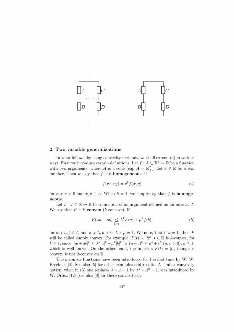
A

B

C

D

A

B

C

D

2. Two variable generalizations

In what follows, by using convexity methods, we shall extend (3) in variousways. First we introduce certain definitions. Let f : A ⊂ R2 → R be a functionwith two arguments, where A is a cone (e.g. A = R2

+). Let k ∈ R be a realnumber. Then we say that f is k-homogeneous, if

f(rx, ry) = rkf(x, y) (4)

for any r > 0 and x, y ∈ A. When k = 1, we simply say that f is homoge-neous.

Let F : I ⊂ R → R be a function of an argument defined on an interval I.We say that F is k-convex (k-concave), if

F (λa+ µb) ≤(≥)

λkF (a) + µkf(b), (5)

for any a, b ∈ I, and any λ, µ > 0, λ+ µ = 1. We note, that if k = 1, then Fwill be called simply convex. For example, F (t) = |t|k, t ∈ R is k-convex, fork ≥ 1, since |λa+µb|k ≤ λk|a|k +µk|b|k by (u+v)k ≤ uk +vk (u, v > 0), k ≥ 1,which is well-known. On the other hand, the function F (t) = |t|, though isconvex, is not 2-convex on R.

The k-convex functions have been introduced for the first time by W. W.Breckner [4]. See also [5] for other examples and results. A similar convexitynotion, when in (5) one replaces λ+ µ = 1 by λk + µk = 1, was introduced byW. Orlicz [12] (see also [8] for these convexities).

447

Now, let A = (0,+∞) × (0,+∞) = R2+ and I = (0,+∞). Define F (t) =

f(1, t) for t ∈ I.Theorem 2. If f is k-homogeneous, and F is k-convex (k-concave) then

f(a1 + · · · + an, b1 + · · · + bn) ≤(≥)

f(a1, b1) + · · · + f(an, bn) (6)

for any ai, bi ∈ A (i = 1, 2, . . . , n).Proof. First remark, that by (4) and the definition of F , one has

akF

(b

a

)= akf

(1,b

a

)= f(a, b) (7)

On the other hand, by induction it can be proved the following Jensen-typeinequality:

F (λ1x1 + λ2x2 + · · · + λnxn) ≤(≥)

λk1F (x1) + λk

2F (x2) + · · · + λknF (xn), (8)

for any xi ∈ I, λi > 0 (i = 1, n), λ1 + · · · + λn = 1.E.g. for n = 3, relation (8) can be proved as follows:

Put a =λ1

λ1 + λ2x1 +

λ2

λ1 + λ2x2, b = x3, λ = λ1 +λ2, µ = λ3 in (5). Then,

as λ1x1 + λ2x2 + λ3x3 = λa+ µb, we have

F (λ1x1 + λ2x2 + λ3x3) ≤ λkF (a) + µkF (b) ≤

≤ (λ1 + λ2)k

[λk

1

(λ1 + λ2)kF (x1) +

λk2

(λ1 + λ2)kF (x2)

]+ λk

3F (x3) =

= λk1F (x1) + λk

2F (x2) + λk3F (x3).

Put now in (8)

x1 =b1a1, x2 =

b2a2, . . . , xn =

bnan,

λ1 =a1

a1 + · · · + an, λ2 =

a2

a1 + · · · + an, . . . , λn =

an

a1 + · · · + an

in order to obtain

F

(b1 + · · · + bna1 + · · · + an

)≤(≥)

ak1F

(b1a1

)+ ak

2F

(b2a2

)+ · · · + ak

nF

(bnan

)

(a1 + · · · + an)k(9)

448

Now, by (7) this gives f(a1 + · · · + an, b1 + · · · + bn) ≤ f(a1, b1) + · · · +f(an, bn), i.e. relation (6).

Remark. Let f(a, b) =a+ b

ab. Then f is homogeneous (i.e. k = 1), and

F (t) = f(1, t) =t+ 1

tis 1-convex (i.e., convex), since F ′′(t) = 2/t3 > 0. Then

relation (6) gives the following inequality:

1

H(a1 + · · · + an, b1 + · · · + bn)≤ 1

H(a1, b1)+ · · · + 1

H(an, bn). (10)

Let now f(a, b) =ab

a+ b. Then f is homogeneous, with F (t) =

t

t+ 1, which

is concave. From (6) (with ≥ inequality), we recapture Lehman’s inequality(3).

The following theorem has a similar proof:Theorem 3. Let f be k-homogeneous, and suppose that F is l-convex

(l-concave) (k, l ∈ R). Then

(a1 + · · · + an)l−kf(a1 + · · · + an, b1 + · · · + bn) ≤ (≥)

al−k1 f(a1, b1) + · · · + al−k

n f(an, bn). (11)

Remarks. For k = l, (11) gives (9).

For example, let f(a, b) =a

b, where a, b ∈ (0,∞) × (0,∞). Then k = 0

(i.e. f is homogeneous of order 0), and F (t) =1

t, which is 1-convex, since

F ′′(t) =2

t3> 0. Thus l = 1, and relation (11) gives the inequality

(a1 + · · · + an)2

b1 + · · · + bn≤ a2

1

b1+ · · · + a2

n

bn(12)

Finally, we given another example of this type. Put f(a, b) =a2 + b2

a+ b.

Then k = 1. Since F (t) =t2 + 1

t+ 1, after elementary computations, F ′′(t) =

4/(t+ 1)3 > 0, so l = 1, and (11) (or (9)) gives the relation

(a1 + · · · + an)2 + (b1 + · · · + bn)2

a1 + · · · + an + b1 + · · · + bn≤ a2

1 + b21a1 + b1

+ · · · + a2n + b2nan + bn

(13)

449

Since L1(a, b) =a2 + b2

a+ b(more generally, Lp(a, b) =

ap+1 + bp+1

ap + bp) are the

so-called ”Lehmer means” [9], [7], [1] of a, b > 0, (13) can be written also as

L1(a1 + · · · + an, b1 + · · · + bn) ≤ L1(a1, b1) + · · · + L1(an, b1). (14)

Clearly, one can obtain more general forms for Lp. For inequalities on moregeneral means (e.g. Gini means), see [10], [11].

3. Holder’s inequality

As we have seen, there are many applications to Theorems 2 and 3. Herewe wish to give an important application; namely a new proof of Holder’sinequality (one of the most important inequalities in Mathematics).

Let f(a, b) = a1/pb1/q, where 1/p + 1/q = 1 (p > 1). Then clearly f

is homogeneous (k = 1), with F (t) = t1/q. Since F ′(t) =1

qt−1/p, F ′′(t) =

− 1

pqt−(1/p)−1 < 0, so by Theorem 2 one gets

(a1 + · · · + an)1/p(b1 + · · · + bn)1/q ≥ a1/p1 b

1/q1 + · · · + a1/p

n b1/qn (15)

Replace now ai = Api , bi = Bq

i (i = 1, n) in order to get

n∑

i=1

AiBi ≤(

n∑

i=1

Api

)1/p( n∑

i=1

Bqi

)1/q

, (16)

which is the classical Holder inequality.

4. Many variables generalization

Let f : A ⊂ Rn+ → R be of n arguments (n ≥ 2). For simplicity, put

p = (x1, . . . , xn), p′ = (x′1, . . . , x′n), when p + p′ = (x1 + x′1, . . . , xn + x′n)

and rp = (rx1, . . . , rxn) for r ∈ R. Then the definitions of k-homogeneityand k-convexity can be extended to this case, similarly to paragraph 2. IfA is a cone, then f is k-homogeneous, if f(rp) = rkf(p) (r > 0) and ifA is convex set then f is k-convex, if f(λp + µp′) ≤ λkf(p) + µkf(p′) forany p, p′ ∈ A, λ, µ > 0, λ + µ = 1. We say that f is k-Jensen convex, if

f

(p+ p′

2

)≤ f(p) + f(p′)

2k. We say that f is r-subhomogeneous of order

k, if f(rp) ≤ rkf(p). Particularly, if k = 1 (i.e. f(rp) ≤ rf(p)), we say that fis r-subhomogeneous (see e.g. [14], [15]). If f is r-subhomogeneous of order

450

k for any r > 1, we say that f is subhomogeneous of order k. For k = 1,see [13]. We say that f is subadditive on A, if

f(p+ p′) ≤ f(p) + f(p′) (17)

We note that in the particular case of n = 2, inequality (6) with ”≤” saysexactly that f(a, b) of two arguments is subadditive.

Theorem 4. If f is homogeneous of order k, then f is subadditive if andonly if it is k-Jensen convex.

Proof. If f is subadditive, i.e. f(p + p′) ≤ f(p) + f(p′) for any p, p′ ∈ A,then

f

(p+ p′

2

)=

1

2kf(p+ p′) ≤ f(p) + f(p′)

2k,

so f is k-Jensen convex. Reciprocally, if f is k-Jensen convex, then

f

(p+ p′

2

)≤ f(p) + f(p′)

2k,

so

f(p+ p′) = f

[2

(p+ p′

2

)]= 2kf

(p+ p′

2

)≤ f(p) + f(p′),

i.e. (17) follows.Remark. Particularly, a homogeneous subadditive function is convex, a

simple, but very useful result in the theory of convex bodies (e.g. ”distancefunction”, ”supporting function”, see e.g. [3], [16]).

Theorem 5. If f is 2-subhomogeneous of order k, and is k-Jensen convex,then it is subadditive.

Proof. Since

f(p+ p′) = f

(2

(p+ p′

2

))≤ 2kf

(p+ p′

2

),

and

f

(p+ p′

2

)≤ f(p) + f(p′)

2k,

we get f(p+ p′) ≤ f(p) + f(p′), so (17) follows.Remark. Particularly, if f is 2-subhomogeneous, and Jensen convex, then

it is subadditive. (18)It is well-known that a continuous Jensen convex function (defined on an

open convex set A ⊂ Rn) is convex. Similarly, for continuous k-Jensen convexfunctions, see [4].

451

To give an interesting example, connected with Lehman’s inequality, let us

consider A = Rn+, f(p) = H(p) = n/

(1

x1+ · · · + 1

xn

).

Let1

g(p)=

1

x1+ · · · + 1

xn. Then

dg

g2=

n∑

i=1

dxi

x2i

,d2g

g2− 2

dg2

g3= −2

n∑

i=1

dx2i

x3i

,

so

1

2

d2g

g3=

(n∑

i=1

dxi

x2i

)2

−(

n∑

i=1

1

xi

)(n∑

i=1

dx2i

x3i

)

.

(Here d denotes a differential.) Now apply Holder’s inequality (16) for p = q =2 (i.e. Cauchy-Bunjakovski inequality), Ai = 1/

√xi, Bi = (1/xi

√xi)dxi. Then

one obtainsd2g

g3≤ 0, and since g > 0, we get d2g ≤ 0. It is well-known ([16])

that this implies the concavity of function g(p) = H(p)/n, so −H(p) will be aconvex function. By consequence (17) of Theorem 5, H(p) is subadditive, i.e.

H(x1 + x′1, x2 + x′2, . . . , xn + x′n) ≥ H(x1, x2, . . . , xn)+

+H(x′1, x′2, . . . , x

′n), (xi, x

′i > 0). (19)

For n = 2 this coincides with (3), i.e. Lehman’s inequality (1).Finally, we prove a result, which is a sort of reciprocal to Theorem 5:Theorem 6. Let us suppose that f is subadditive, and k-convex, where

k ≥ 1. Then f is subhomogeneous of order k.Proof. For any r > 1 one can find a positive integer n such that r ∈

[n, n + 1]. Then r can be written as a convex combination of n and n + 1:r = nλ+ (n+ 1)µ. By the k-convexity of f one has

f(rp) = f(nλp+ (n+ 1)µp) ≤ λkf(np) + µkf [(n+ 1)p].

Since f is subadditive, from (17) it follows by induction that f(np) ≤ nf(p),so we get

f(rp) ≤ nλkf(p) + (n+ 1)µkf(p) = [nλk + (n+ 1)µk]f(p).

Now, since k ≥ 1, it is well-known that

[λn+ (n+ 1)µ]k ≥ (λn)k + ((n+ 1)µ)k.

452

But (λn)k ≥ nλk and ((n+ 1)µ)k ≥ (n+ 1)µk, so finally we can write

f(rp) ≤ [λn+ (n+ 1)µ]kf(p) = rkf(p),

which means that f is subhomogeneous of order k.Remark. For k = 1 Theorem 6 contains a result by R. A. Rosenbaum

[13].Acknowledgments. The author thanks Professors J. Peetre and H. Alzer

for providing their reprints [2], resp. [1]. He is indebted to Professor F. A.Valentine for a copy of his book [16], and also to Professors W. W. Brecknerof Cluj, and V. E. Szabo of Budapest for helpful discussions.

NOTE ADDED IN PROOF. Recently (23th February, 2005) we have dis-covered that Lehman’s inequality (2) (or (3)) appears also as Theorem 67 inG. H. Hardy, J. E. Littlewood and G. Polya [Inequalities, Cambridge Univ.Press, 1964; see p.61], and is due to E. A. Milne [Note on Rosseland’s inte-gral for the stellar absorption coefficient, Monthly Notices, R.A.S. 85(1925),979-984]. Though we are unable to read Milne’s paper, perhaps we should callLehman’s inequality as the ”Milne-Lehman inequality”. We note also that theMilne-Lehman inequality is published as a Proposed Problem 2113 (by M.E.Kuczma), as well as Problem 2392 (by G. Tsintsifas) in the Canadian journalCrux Mathematicorum.

References

[1] H. Alzer, Uber Lehmers Mittelwertfamilie, Elem. Math., 43(1988), no.2, 50-54.

[2] J. Arazy, T. Claesson, S. Janson and J. Peetre, Means and their iteration,Proc. 19th Nordic Congr. Math., Reykjavik 1984, 191-212.

[3] T. Bonnesen and W. Fenchel, Theorie der konvexen Korper, Berlin, 1934.

[4] W. W. Breckner, Stetigkeitsaussagen fur eine Klasse verallgemeinerterkonvexer Funktionen in topologischen linearen Raume, Publ. Inst. Math.(Beograd), 23(1978), 13-20.

[5] W. W. Breckner and Gh. Orban, Continuity properties of rationally s-convex mappings with values in an ordered topological linear space, 92pp., Babes-Bolyai Univ., Cluj, Romania, 1978.

[6] R. J. Duffin, Network models, in SIAM-AMS Proceedings vol. III, pp.65-91, AMS, Providence, 1971.

453

[7] H. W. Gould and M. E. Mays, Series expansions of means, J. Math.Anal. Appl., 101(1984), 611-621.

[8] H. Hudzik and L. Maligranda, Some remarks on s-convex functions, Ae-quationes Math., 48(1994), 100-111.

[9] D. H. Lehmer, On the compounding of certain means, J. Math. Anal.Appl., 36(1971), 183-200.

[10] E. Neuman and J. Sandor, Inequalities involving Stolarsky and Ginimeans, Math. Pannonica 14(2003), 29-44.

[11] E. Neuman and J. Sandor, On certain new means of two arguments andtheir extensions, Int. J. Math. Math. Sci., 16(2003), 981-993.

[12] W. Orlich, A note on modular spaces, I, Bull. Acad. Polon. Sci. Ser. Sci.Math. Astronom. Phys., 9(1961), 157-162.

[13] R. A. Rosenbaum, Subadditive functions, Duke Math. J., 17(1950), 227-247.

[14] J. Sandor and Gh. Toader, On some exponential means, Babes-BolyaiUniv., Preprint No. 7, 1990, 35-40.

[15] J. Sandor, On certain subhomogeneous means, Octogon Math. Mag.,8(2000), 156-160.

[16] F. A. Valentine, Convex sets, Mc Graw-Hill Inc., New York, 1964.

454

Author Index

AS. Arslanagic 1.4, 4.4H. Alzer 2.1, 2.10, 4.9, 4.10, 4.16, 5.12,6.3, 6.4, 6.10, 6.13, 6.14, 6.15, 10.9,10.10J.L. d’Alambert 2.5T.M. Apostol 3.7, 9.10Ch. Ashbacher 3.11, 3.12, 3.17, 9.16W. Aiello 3.19E. Artin 5.9, 5.11, 5.13, 5.15, 6.11, 7.1R.P. Agarwal 5.13M. Abramowitz 5.13C. Alsina 5.15J. Arazy 6.3, 10.10R. Askey 7.1J. Aczel 7.2, 7.4, 7.5D. Acu 7.2T. Andreescu 8.3D. Andrica 8.3C. Adiga 9.4L. Alaoglu 9.7K.T. Atanassov 9.14, 10.8

BE. Bezout 1.2M. Bencze 1.5, 1.8, 1.11, 1.12, 2.2A,2.2B, 2.2C, 2.2G, 2.2H, 2.2J, 2.2S,2.2T, 2.2U, 2.3, 2.9, 3.9, 3.10, 3.14,4.13, 5.5, 5.6, 5.14, 8.3, 8.9, 9.6, 9.9

O. Bottema 1.5, 1.6H. Brocard 1.6D.M. Batinetu-Giurgiu 1.8, 2.2A,2.2L, 2.2M, 2.2N, 2,2O, 2.2P, 2.2S,2.2T, 5.5, 5.6, 5.7H.J. Brothers 2.1, 2.2F, 2.2PJ. Bernoulli 2.2I, 2.2J, 3.7, 5.3V. Berinde 2.5T.J. Bromwich 2.5Gy. Bereznai 2.6N.G. de Bruijn 2.7F. Bencherif 2.7D. Bradley 2.9G.M. Bell 2.9T. Bonnesen 10.10G. Bennett 2.10, 5.12A. Balog 3.2D. Bode 3.9R. Bojanic 3.16A. Bege 3.19V. Bunjakovski (Bunyakovsky) 4.2,4.4, 6.6, 10.10E.F. Beckenbach 4.14R. Bellman 4.14H. Bohr 5.9, 5.13, 7.1J. Bass 5.11J. Bursuc 5.11N.S. Barnett 5.13C.W. Borchardt 6.7

455

O. Bonnett 6.16M. Balazs 6.16V. Bandila 7.2B. Bartha 7.9A. Bremner 8.6J.M. Brown 10.3W.W. Breckner 10.10

CR. Cotes 1.2L. Cauchy 1.5, 2.2H, 2.10, 4.2, 4.4,4.16, 6.6, 6.10, 6.13, 6.15, 7.1, 7.3, 7.4,7.5, 7.6, 10.10L. Carlitz 1.6F.T. Campan 1.14N. de Cusa 1.14E. Cesaro 2.2I, 2.2O, 2.2R, 2.3A, 2.3BJ.H. Conway 2.2UJ. Choi 2.9E. Catalan 2.9B. Crstici 3.1, 3.2, 5.15, 9.1, 9.2, 10.2W. Chen 3.8H.Z. Cao 3.8G.L. Cohen 3.19, 10.7G. Chrystal 4.3, 4.4P. Chebyshev 4.10, 4.11, 7.10M. Craiu 5.11, 6.16M.J. Cloud 5.16B.C. Carlson 6.3, 6.7, 6.11T. Claeson 6.7, 10.10C.-P. Chen 6.13G. Chilov 6.16C.V. Craciun 6.16R.O. Cuzmin 6.16N. Cioranescu 7.4B. Conn 8.6E. Cohen 9.6, 9.10, 9.11I. Creanga 9.7

D

L. Denbath 2.2PG.L. Dirichlet 2.9, 9.7, 9.14S.S. Dragomir 2.10, 4.9, 4.10, 5.13P. Dusart 3.2F.W. Dodd 3.8R. Dedekind 3.13, 8.12, 8.13, 8.14L.E. Dickson 3.13M. Deng 3.19B.P. Demidovich 5.11, 6.11B.C. Drachman 5.16J. Dieudonne 6.14G. Darboux 6.15, 6.16R.J. Duffin 10.10

EP. Erdos 1.3, 1.9. 9.3, 9.7, 9.14L. Euler 1.5, 2.2J, 2.2K, 2.2M, 2.2O,2.2Q, 2.3, 2.6, 2.9, 2.10, 3.7, 3.11, 3.12,3.13, 5.1, 5.2, 5.4, 5.5, 5.7, 5.11, 6.11,6.16, 8.11, 8.12, 8.13, 9.7, 9.8, 9.14,10.4A. Erdelyi 2.4Euclid of Alexandria 3.12, 10.2J. Earls 3.15, 3.16, 3.17, 3.18, 8.16,10.5

FP. Fermat 1.2, 3.17, 10.2B. Finta 1.3J.B. Fourier 1.11S. Finch 2.1L. Filep 2.6K. Ford 3.15J. Findley 3.15J. Fabrykowski 3.19A.M. Fink 4.12K. Fan 4.13, 4.14, 6.10, 10.9J. Frauenthal 5.16A.N. Fathima 9.4W. Fenchel 10.10

456

GM. Ghermanescu 2.1, 2.2O, 2.2PG. Garnir 2.2I, 2.2RR.K. Guy 3.4, 8.1, 8.6, 8.15, 10.7P. Gronas 3.12K.F. Gauss 3.12, 3.13, 5.4, 6.3, 6.7,9.6, 10.2S.W. Golomb 3.13J. Galambos 3.14W. Gautschi 5.13B. Gelbaum 6.14N.M. Gunther 6.16R.R. Goldberg 6.16V.L. Gardiner 8.6C. Gini 10.9, 10.10H.W. Gould 10.10

HHeron of AlexandriaJ. Hadamard 1.11, 2.1, 4.7, 4.8, 4.9,4.10, 5.11, 5.13, 6.9, 9.11, 9.13Ch. Hermite 1.11, 4.7, 5.13G. de l’Hopital 1.15, 2.1, 2.2RD.R. Hofstadter 2.2UG.H. Hardy 2.9, 2.10, 3.9, 4.3, 4.11,4.14, 5.13, 6.10, 6.14, 8.1, 9.6, 9.7,9.10, 9.11, 10.3J. Van der Hoek 2.10M. Hazewinkel 3.14P. Hagis 3.19J. Hanumanthachari 3.19O. Holder 5.13, 5.14, 7.1, 10.10V. Hiris 6.16S. Haruki 7.4D.R. Heath-Brown 8.6M. Hausman 9.2H. Hudzik 10.10

IA. Ivic 3.19, 9.6

R. Ianic 7.2

JC. Jordan 1.4, 1.11, 6.7, 9.7J.L. Jensen 1.11, 4.7, 4.9, 5.13, 7.4,9.11, 9.13, 10.9, 10.10W. Janous 1.12, 3.1S. Janson 6.7, 10.10F.H. Jackson 7.1

KN.D. Kazarinoff 1.9J.A. Knox 2.1, 2.2F, 2.2OK. Knopp 2.8H.M. Korobov 3.4H.J. Kanold 3.9, 3.10I. Katai 3.14J.M. DeKoninck 3.19, 9.6, 9.10N. Keyfitz 5.16F. Klein 6.4J. Karamata 6.5J. Kolumban 6.16K. Koyama 8.6T. Kim 9.4M.S. Klamkin 9.11, 10.3K. Kashihara 9.16E. Kratzel 10.3

LP.S. Laplace 6.16T. Lalescu 1.6, 5.1, 5.12F. Leuenberger 1.6E. Lemoine 1.6J. Lagrange 2.2Q, 2.10, 4.9, 5.2, 6.7,6.9, 6.11D.A. Lavis 2.9J.E. Littlewood 2.10, 3.4, 4.3, 4.11,4.14, 5.13, 6.10, 6.14G.G. Lorentz 2.10G. Lord 3.19

457

L. Lucht 3.19T.P. Lin 4.7, 6.3A.M. Legendre 5.4A. Lupas 5.11J. Lew 5.16A. Lehman 10.10D.H. Lehmer 10.10E.B. Leach 6.2, 6.3, 6.5, 6.7H. Lebesgue 7.1F. Luca 9.14, 10.8C.C. Lindner 10.8E.S. Langford 9.11B. Lepson 10.3W.M. Lioen 8.6R.F. Lukes 8.6R.B. Lazarus 8.6R. Lipschitz 9.1M. Lee 9.2, 9.14, 10.8R. Laatsch 9.2E. Lucas 9.8

MD.S. Mitrinovic 1.4, 1.5, 1.11, 1.13,1.16, 2.10, 3.1, 3.2, 3.4, 3.8, 4.10, 4.12,5.8, 5.10, 5.11, 5.15, 6.11, 7.1, 9.1, 9.2,9.6, 9.11, 10.3D.M. Milosevic 1.4, 1.5, 4.10H. Minc 2.10, 5.11R.K. Meany 10.3Gy. Maurer 1.2K.B. Mollweide 1.7L.J. Mordell 1.9A.W. Marshall 1.12C. Maclaurin 2.2H, 2.3A, 6.10A. Murthy 2.8, 3.15, 9.2, 9.3, 9.6J.S. Martins 2.10L.E. Matties 3.8A.P. Minin 3.13P. Mersenne 3.15J. Mollerup 4.9, 5.13, 7.1

L. Maligranda 10.10I.A. Maron 5.11, 6.11M. Megan 6.16J.C.P. Miller 8.6L.J. Mordell 8.6P. Moree 9.3, 9.14, 9.15, 10.8A. Mobius 9.7A. Makowski 9.10J. Morgado 9.10M.E. Mays 10.10J.C. Maxwell 10.10

NC. Nedelcu 1.4T. Negoi 2.2FJ. Nagura 3.5C.A. Nicol 3.13, 8.11K. Nageswara Rao 3.19E. Neuman 4.13, 10.9, 10.10S.M. Nikolsky 6.16T. Nagell 8.4A. Nikiforov 5.15

OM. Olteanu 1.10I. Olkin 1.12L. Olivier 2.8O. Ore 3.19, 10.7J.M.H. Olmsted 6.14W. Orlicz 10.10Gh. Orban 10.10V. Ouvarov 5.15

PJ.E. Pecaric 1.5, 4.9, 4.10, 7.2G. Polya 1.6, 2.10, 4.3, 4.11, 4.14, 5.13,6.10, 6.14, 9.7D. Pedoe 1.6A.O. Pittenger 2.1, 6.3, 10.9T. Popoviciu 2.1

458

I.I. Pjateckii-Sapiro 3.2F. Popovici 3.9J.L. Pe 3.12, 3.13M. Petrovic 5.9J. Peetre 6.7, 10.10C. Popa 6.16E. Prouchet 9.8C. Pomerance 9.10

QF. Qi 6.13

RR. Redheffer 1.4, 1.11, 1.13G. Robin 2.7S. Ramanujan 2.9, 6.5, 9.6J.B. Rosser 3.1, 3.2, 3.6B. Riemann 3.4, 3.7, 5.5, 6.16, 9.7I.Z. Ruzsa 3.10, 9.11A.W. Roberts 4.3, 4.15, 6.15J.L. Raabe 5.11I. Rasa 6.3, 6.6, 10.9M. Rolle 6.11, 6.14, 6.15W. Rudin 6.14M.N. Rosculet 5.11, 6.16Th. M. Rassias 7.8, 7.12, 8.2, 8.5, 8.6H.J.J. te Riele 8.6H. Roskam 9.14, 9.15, 10.8J. Rooin 10.9R.A. Rosenbaum 10.10P. du Bois-Reymond 6.16

SJ. Sandor 1.3, 1.4, 1.5, 1.6, 1.8, 1.9,1.10, 1.11, 1.13, 1.14, 2.1, 2.2A, 2.2B,2.2C, 2.2D, 2.2F, 2.2H, 2.2J, 2.2O,2.2P, 2.2S, 2.5, 2.9, 2.10, 3.1, 3.2, 3.4,3.6, 3.7, 3.8, 3.9, 3.10, 3.11, 3.12, 3.13,3.14, 3.16, 3.19, 4.3, 4.7, 4.8, 4.9, 4.10,4.11, 4.15, 4.16, 5.5, 5.7, 5.8, 5.10,

5.11, 5.13, 5.14, 5.15, 6.1, 6.2, 6.3, 6.4,6.6, 6.7, 6.8, 6.9, 6.10, 6.11, 6.13, 6.14,6.15, 6.16, 7.2, 7.4, 7.5, 7.11, 8.1, 8.6,8.9, 8.11, 8.12, 8.14, 8.15, 9.1, 9.3, 9.4,9.5, 9.7, 9.10, 9.11, 9.13, 9.14, 9.15,9.16, 10.2, 10.3, 10.4, 10.7G. Szego 1.6, 9.7S.B. Steckin 1.11W. Snellius 1.14K.B. Stolarsky 2.1, 4.9, 6.3, 6.7, 10.3,10.10Gh. Stoica 2.1O. Stolz 2.2I, 2.2O, 2.2Q, 2.3A, 2.3BI. Sathre 2.10, 5.11I. Schoenfeld 3.1, 3.2, 3.6J. Stirling 3.7, 5.5D. Suryanarayana 3.9, 3.10I. Smarandache 3.9, 3.11, 3.12, 3.15,3.17, 8.1, 8.13, 8.16, 9.4, 9.5, 9.13,9.14, 9.15, 9.16, 10.5I. A. Stegun 5.13R.M. Sorli 3.19, 10.7E.G. Straus 3.19, 9.13M.V. Subbarao 3.19, 9.13H.J. Seiffert 6.1, 6.3, 6.4, 6.8V.E.S. Szabo 6.1, 6.2, 6.3M.C. Sholander 6.2, 6.3, 6.5, 6.7J. Steiner 6.4H. Shniad 6.5W. Sierpinski 6.10, 7.3, 9.3, 9.9E.L. Stark 6.16I. Stamate 7.2H.N. Shapiro 7.3, 9.8K.B. Subramanian 8.4P.R. Stein 8.6H. Sekigawa 8.6D.D. Somashekara 9.4A. Schinzel 9.10, 9.14A. Stenger 10.3

459

TD.W. De Tempe 2.2FS.R. Tims 2.2FJ.A. Tyrrel 2.2FF. Tricomi 2.4L. Toth 2.4, 5.12, 9.10, 9.11B. Taylor 3.7, 6.11, 6.15, 6.16Gh. Toader 4.9, 4.10, 4.11, 6.3, 6.6,6.9, 10.10T. Trif 4.13, 10.9M.S. Tomas 5.15J. Thomae 7.1Y. Tsuruoka 8.6Z. Tuzson 8.6E.C. Titchmarsh 9.7

VI. Virag 1.2V. Volenec 1.5A. Vernescu 2.4Ch.J. de la Vallee-Poussin 3.4P. Vlamos 3.6D.E. Varberg 4.3, 4.15, 6.15M. Vuorinen 5.14, 6.2, 6.3, 6.7M.K. Vamanamurthy 6.2, 6.3, 6.7M. Vlada 7.2I.M. Vinogradov 8.3L. Vaserstein 8.6

F.A. Valentine 10.10

WR. WeitzenbockJ. Wallis 2.4E.M. Wright 3.9, 8.1, 9.7, 9.10, 9.11,10.3Ch. Wall 3.19E.T. Whittaker 5.3, 5.4, 5.5, 5.6, 5.11,5.14, 5.15, 5.16, 6.16G.N. Watson 5.3, 5.4, 5.5, 5.6, 5.11,5.14, 5.15, 5.16, 6.16K. Weierstrass 5.11, 6.16J. Wendel 5.13, 5.14, 5.16D. Widder 6.16R. Webster 7.1D.T.Walker 8.3, 8.4M.F.C. Woollett 8.6W.-L. Wang 10.9P.-F. Wang 10.9

YW.H. Young 5.10

ZA. Zygmund 6.16P. Zwier 10.3

460

Documents

SELECTED CHAPTERS OF GEOMETY, ANALYSIS AND NUMBER THEORY · PDF fileSELECTED CHAPTERS OF GEOMETY, ANALYSIS AND NUMBER THEORY by ... Bernoulli numbers, perfect numbers and generalizations,

References

[1] M. Bencze, OQ.860, Octogon Math. Mag., 10(2002), no.1, 517.
[1] M. Bencze, OQ.896, Octogon Math. Mag., 10(2002), no.1, 525.
[2] J. Sandor, On the Open Problem OQ.803, Octogon Math. Mag., 10(2002), no.1, 413-414.
[3] J. Sandor, On OQ.896, Octogon Math. Mag., 11(2003), no.1, 233.
[1] D.M. Batinetu-Giurgiu, OQ.999, Octogon Math. Mag., 10(2002), no.1,1047.
[1] D.M. Batinetu-Giurgiu, OQ.994, Octogon Math. Mag., 10(2002), no.1,1046.
[2] J. Sandor, On the Open Problem OQ.994, Octogon Math. Mag., 11(2003), no.1, 252-253.
[1] D.M. Batinetu-Giurgiu, OQ.1007, Octogon Math. Mag., 10(2002), no.2,1049.
[1] M. Bencze, OQ.813, Octogon Math. Mag., 10(2002), no.1, 507.
[1] M. Bencze, OQ.809, Octogon Math. Mag., 10(2002), no.1, 506.
[2] J. Sandor, On OQ.809, Octogon Math. Mag., 11(2003), no.1, 224.
[1] M. Bencze, OQ.818, Octogon Math. Mag., 10(2002), no.1, 507.
[1] M. Bencze, OQ.546, Octogon Math. Mag., 8(2000), no.2, 625.
[1] M. Bencze, OQ.608, Octogon Math. Mag., 9(2001), no.1, 673.
[1] M. Bencze, OQ.612, Octogon Math. Mag., 9(2001), no.1, 674.
[1] M. Bencze, OQ.528, Octogon Math. Mag., 8(2002), no.2, 622.
[1] M. Bencze, OQ.1352, Octogon Math. Mag., 12(2004), no.1, 448.
[1] M. Bencze, OQ.1074, Octogon Math. Mag., 10(2002), no.2, 1064.
[1] Th.M. Rassias, OQ.725, Octogon Math. Mag., 9(2001), no.2, 1084.
[1] Th.M. Rassias, OQ.277, Octogon Math. Mag., 7(1999), no.2, 195.
[1] M. Bencze, OQ.1119, Octogon Math. Mag., 10(2002), no.2, 1075.
[1] M. Bencze, OQ.753, Octogon Math. Mag., 9(2001), no.2, 1088.
[1] M. Bencze, OQ.1284, Octogon Math. Mag., 11(2003), no.2, 851.