Christian Pelties & Martin Käser

Department of Earth and Environmental Sciences, LMU München, Germany

SeisSolSeisSol PracticalsPracticals

February 20th-25th, 2011

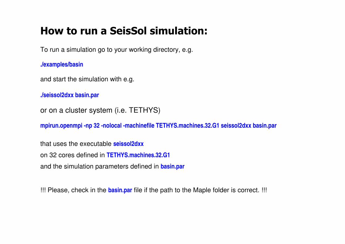
How to run a SeisSol simulation:

To run a simulation go to your working directory, e.g.

./examples/basin

and start the simulation with e.g.

./seissol2dxx basin.par

or on a cluster system (i.e. TETHYS)

mpirun.openmpi -np 32 -nolocal -machinefile TETHYS.machines.32.G1 seissol2dxx basin.par

that uses the executable seissol2dxx

on 32 cores defined in TETHYS.machines.32.G1

and the simulation parameters defined in basin.par

!!! Please, check in the basin.par file if the path to the Maple folder is correct. !!!

Output files generated by a SeisSol simulation:

Each core writes its

log-file: IRREGULARITIES.0000.log

progress-file: StdOut0000.txt

seismograms: output-pickpoint-00001-0000.dat

( = time series of seismic ground motion at one postion in space )

snapshots: output-000000000.0000.tri.dat

( = spatial slice of seismic ground motion on mesh vertices

at one position in time )

snapshots fine-output: output.GF.000000000.0000.dat

( = spatial slice of seismic ground motion as polynomialcoefficients in each element at one position in time )

���� the snapshot fine-output has to be post-processedfor visualization on an additional, regular,

fine visualization grid

���� the post-processing is done with dgvisuxx

number of core

number of receiver

number of time step

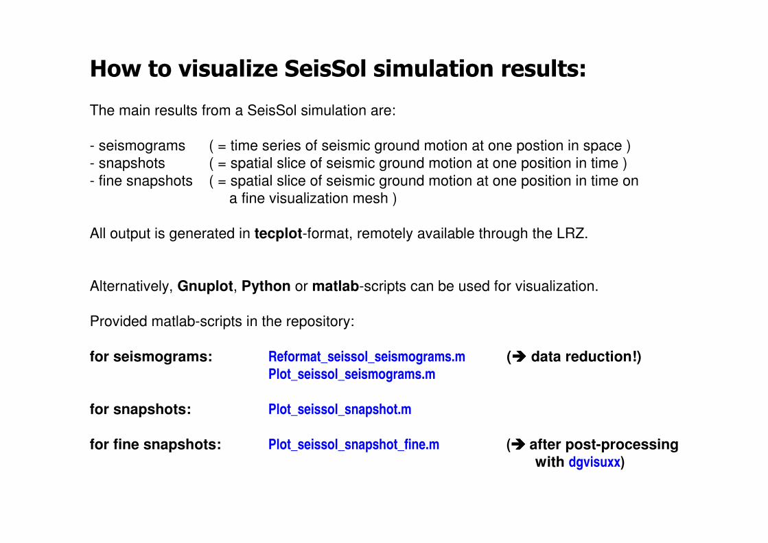
How to visualize SeisSol simulation results:

The main results from a SeisSol simulation are:

- seismograms ( = time series of seismic ground motion at one postion in space )

- snapshots ( = spatial slice of seismic ground motion at one position in time )

- fine snapshots ( = spatial slice of seismic ground motion at one position in time on

a fine visualization mesh )

All output is generated in tecplot-format, remotely available through the LRZ.

Alternatively, Gnuplot, Python or matlab-scripts can be used for visualization.

Provided matlab-scripts in the repository:

for seismograms: Reformat_seissol_seismograms.m (���� data reduction!)

Plot_seissol_seismograms.m

for snapshots: Plot_seissol_snapshot.m

for fine snapshots: Plot_seissol_snapshot_fine.m (���� after post-processing

with dgvisuxx)

Post-Processing of Galerkin Fine (GF) output:

The Galerkin Fine (GF) output contains the polynomial coefficients of the approximation

for every element.

Therefore, the resolution can be much higher through the element-internal structure

of the wave field than for the normal snapshot output.

dgvisuxx is a tool to evaluate the polynomial approximation on a user-definedregular visualization grid

The required input file (e.g. visu_basin.in) can have the following form:

1 ! Cartesian mode (yes=1)

-12000. -7000. 0. ! Coordinates of origin

30000. 0. 0. ! Vector of 1st Cartesian axis

0. 7000. 0. ! Vector of 2nd Cartesian axis

400 ! Number of samples on 1st axis

100 ! Number of samples on 2nd axis

1 ! MPI input data (no=0, yes=1)

32 ! Number of CPUs

output.GF.000000000 ! MPI root filename

GF_basin.dat ! Output file name

1 ! Output format (Tecplot=1)

sigma_xx ! Variable name 1

sigma_yy ! Variable name 2

sigma_xy ! Variable name 3

u ! Variable name 4

v ! Variable name 5

0 ! End of file indicator

Create a file called DGPATH in your

working directory, containing the absolute

path to your Maple directory, e.g.

/home/messuser/seissol2d/Maple/

Then execute the post-processing via:

./dgvisuxx < visu_basin.in

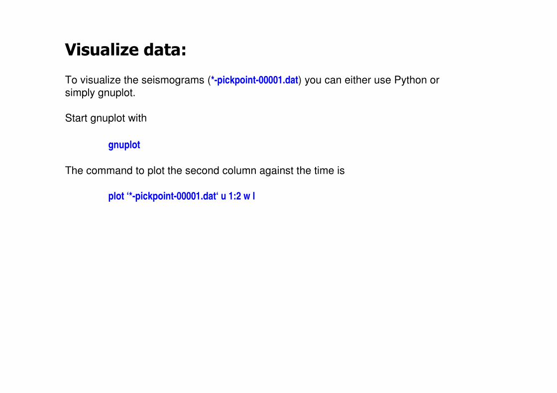
Visualize data:

To visualize the seismograms (*-pickpoint-00001.dat) you can either use Python or

simply gnuplot.

Start gnuplot with

gnuplot

The command to plot the second column against the time is

plot ‘*-pickpoint-00001.dat‘ u 1:2 w l

Visualize data:

To visualize the snapshots which include mesh information use:

./visz_snap.py

as follows:

./visz_snap.py output-000000000.tri.dat

You produce a readable fine-output that respects the high-order polynomials

with:

./dgvisuxx < visu.in

The result

GF_output_t0.dat

can be visualized with

./visz_fine.py GF_output_t0.dat

Some useful information…

• If your simulation runs too slow, you can always reduce the order of accuracy to get

a first impression.

• During runtime you can work on the next step in one exercise.

• You can follow the seismogram in real time using gnuplot – press ‘a‘ to update. To

quit gnuplot press ‘q‘.

• Also the snapshots and the fine output can be visualized during runtime.

Excercises (1):

1) Make yourself familiar with the given folder structure in seissol2d.

2) Run the example model „basin“ with the pre-defined setup, i.e.

with the given files .par, .neu, .def.

3) Use gnuplot to visualize the seismograms.

4) Get a rough impression of the wave field after 1 sec simulation time using

visz_snap.py. Where are the receivers located?

5) Get the same time slice of the wave field by post-processing the Galerkin Fine (.GF.)

output with dgvisuxx and visu_basin.in and visualize the wave field using

visz_fine.py.

6) Increase the simulation time to 3 or 4 sec to get longer seismograms.

7) Increase the order of accuracy, re-run the simulation. How does the time step change

with approximation order? What is the effect on the runtime?

8) Compare the seismograms inside and outside the basin. What is your interpretation for

the difference?

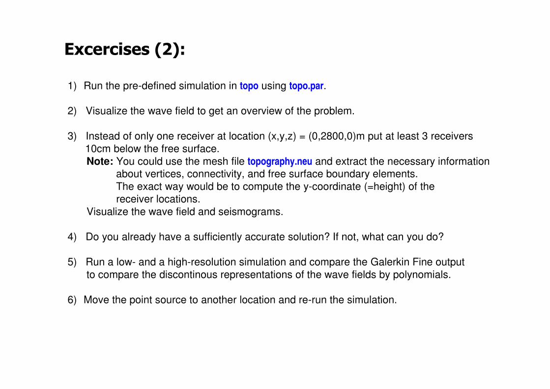
Excercises (2):

1) Run the pre-defined simulation in topo using topo.par.

2) Visualize the wave field to get an overview of the problem.

3) Instead of only one receiver at location (x,y,z) = (0,2800,0)m put at least 3 receivers

10cm below the free surface.

Note: You could use the mesh file topography.neu and extract the necessary informationabout vertices, connectivity, and free surface boundary elements.

The exact way would be to compute the y-coordinate (=height) of the

receiver locations.

Visualize the wave field and seismograms.

4) Do you already have a sufficiently accurate solution? If not, what can you do?

5) Run a low- and a high-resolution simulation and compare the Galerkin Fine output

to compare the discontinous representations of the wave fields by polynomials.

6) Move the point source to another location and re-run the simulation.

Excercises (3):

1) Run the pre-defined simulation in lvz using lvz.par.

2) Visualize the model discretization (mesh). What is different compared to the

previous model discretizations? Is this considered in the *.neu file?

3) Run one example with the pre-defined materials and one with a homogeneous

material model. Observe the differences in the seismograms and/or snapshots.

4) Change the source depth and evaluate its effect on the generation of surface

waves.

5) Change the source type, e.g. from vertical point force to horizontal point force,

or to explosive point source and evaluate its effect on the generation of surface

waves.

Excercises (4):

1) Run the pre-defined simulation in global using global.par.

2) Visualize the model discretization (mesh) and the distribution of the

shear modulus µ. What is the option in global.par to get this material distribution?

3) Visualize the wave field using the Galerkin Fine (.GF.) output and compare the

amplitudes of body and surface waves.

4) Change the source location and visualize the differences in the snapshots and/or

seismograms.

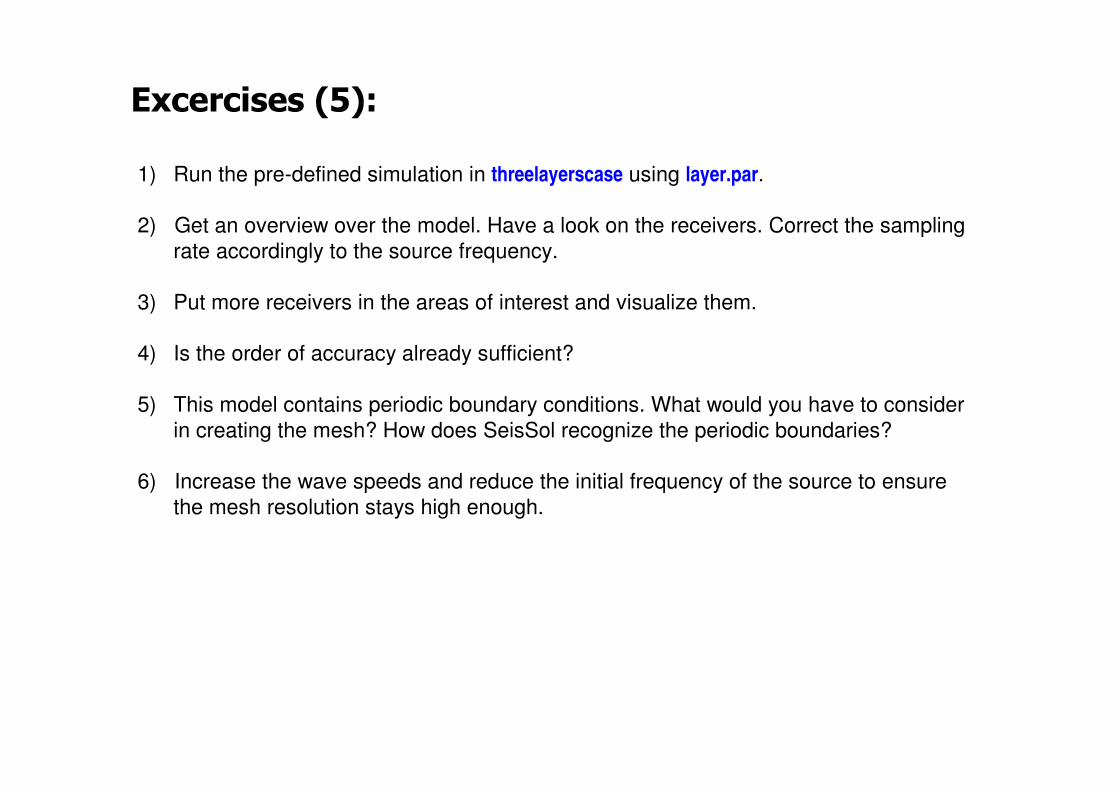
Excercises (5):

1) Run the pre-defined simulation in threelayerscase using layer.par.

2) Get an overview over the model. Have a look on the receivers. Correct the sampling

rate accordingly to the source frequency.

3) Put more receivers in the areas of interest and visualize them.

4) Is the order of accuracy already sufficient?

5) This model contains periodic boundary conditions. What would you have to consider

in creating the mesh? How does SeisSol recognize the periodic boundaries?

6) Increase the wave speeds and reduce the initial frequency of the source to ensure

the mesh resolution stays high enough.

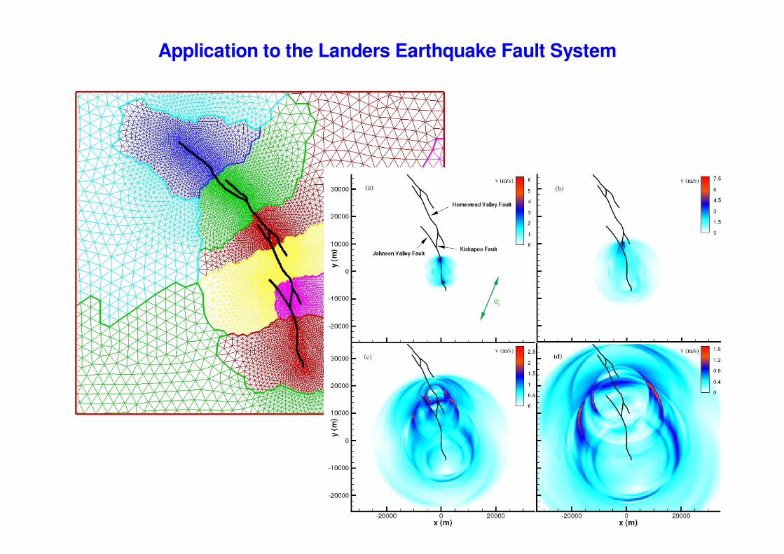
Application to the Landers Earthquake Fault System

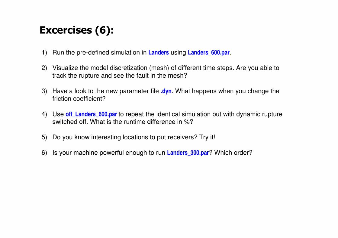
Excercises (6):

1) Run the pre-defined simulation in Landers using Landers_600.par.

2) Visualize the model discretization (mesh) of different time steps. Are you able to

track the rupture and see the fault in the mesh?

3) Have a look to the new parameter file .dyn. What happens when you change thefriction coefficient?

4) Use off_Landers_600.par to repeat the identical simulation but with dynamic ruptureswitched off. What is the runtime difference in %?

5) Do you know interesting locations to put receivers? Try it!

6) Is your machine powerful enough to run Landers_300.par? Which order?