Seismically induced landslide displacements: a predictive ...nceg.uop.edu.pk/workshop-17to31mar-05/Slides/day17/background... · Seismically induced landslide displacements: a predictive

Engineering Geology 58 (2000) 337–351www.elsevier.nl/locate/enggeo

Seismically induced landslide displacements:a predictive model

Roberto Romeo *Servizio Sismico Nazionale (SSN) Via Curtatone 3, I-00185 Rome, Italy

Received 6 November 1998; accepted for publication 16 February 2000

Abstract

Newmark’s model for predicting earthquake-induced landslide displacements provides a simple way to predict thecoseismic displacements affecting a sliding mass subject to earthquake loading. In this model, seismic slope stabilityis measured in terms of critical acceleration, which depends on the mechanical soil properties, pore-pressuredistribution, and slope geometry. The triggering seismic forces are investigated in terms of energy radiation from thesource, propagation, and site effects, based on 190 accelerometric recordings from 17 Italian earthquakes withmagnitudes between 4.5 and 6.8. The method is based on the calibration of relations having the general form of anattenuation law that relates the energy of the seismic forces to the dynamic shear resistances of the sliding mass topropagate the expected landslide displacements as an inverse function of the distance from the fault rupture; theamount of displacement computed through these relations provides a criterion to predict the occurrence of slopefailures. Finally, maps showing, in a deterministic and a probabilistic way, the potential of seismically inducedlandslide displacements are displayed as a tool to provide seismic landslide scenarios and earthquake-induced landslidehazard maps, respectively. © 2000 Elsevier Science B.V. All rights reserved.

Keywords: Attenuation relations; Landslide displacement; Newmark’s method; Probability maps; Seismic hazards

1. Introduction Earthquakes (C.E.D.I.T., release 1.1; Romeo andDelfino, 1997)1.

The stability of slopes subject to earthquakeLandslides are among the most hazardouseffects of earthquakes (Keefer, 1984). This rele- loading can be evaluated using several methods.

Currently most seismic codes, including Italianvance has been further confirmed by the analysesof the earthquake-induced ground failures in Italy and European codes (see ‘Decree of the Italian

Ministry of Public Works March 11, 1988’,based on the historical information about land-slides, surface fracturing and faulting, liquefaction, ‘Eurocode 7: Geotechnical Design’, and ‘Eurocode

8: Design Provisions for Earthquake Resistance ofand topographic changes contained in the NationalCatalogue of Ground Effects Induced by Strong Structures’), use an ultimate-limit-state design cri-

terion for the evaluation of the safety conditions

* Tel.: +39-06-4444-2276. fax: +39-06-4466-579.1 The catalog is available at the following Internet address:E-mail address: [email protected] and fromeo@tiscabi-

net.it (R. Romeo) http://www.dst.it/ssn/RT/rt9704/frameset.html.

0013-7952/00/$ - see front matter © 2000 Elsevier Science B.V. All rights reserved.PII: S0013-7952 ( 00 ) 00042-9

338 R. Romeo / Engineering Geology 58 (2000) 337–351

of embankments and slopes. These can be eval- ation (PGA). All the analyses that follow havebeen carried out using a strong-motion databaseuated through ordinary limit-equilibrium methods

or stress analyses, expressing the stability of a composed of 190 digitized accelerograms (95couples of EW and NS horizontal components)slope in terms of an overall safety factor (SF) or

safety margin (SM), i.e., as the ratio or the differ- from the recordings of 17 Italian earthquakes withmagnitudes ranging from 4.6 to 6.8 (Sabetta andence between available and mobilized shear

strengths. Pugliese, 1996). The acceleration time historiesrequired to be baseline- and instrument-correctedAnother way to express the seismic stability of

a slope is by applying Newmark’s sliding block with a filter in the frequency domain. The bandpassfrequencies (between 0.2 and 0.5 Hz for the high-method (Newmark, 1965), which estimates the

expected coseismic displacements for a given pass filtering and between 25 and 30 Hz for thelow-pass filtering) were selected in order to maxi-recorded or artificial acceleration time history. The

method has undergone several modifications and mize the signal-to-noise ratio. The filtering processreduced the PGA values by an average of aboutimprovements (Sarma, 1981; Wilson and Keefer,

1983), and several relations between seismic 3%. For each record, the epicentral distance (RE)and the closest distance to the surface projectionground-motion parameters and computed land-

slide displacements have been proposed of the fault rupture (RF) are provided. Eachrecording site is also classified as rock (firm soil )(Ambraseys and Menu, 1988; Jibson, 1993;

Ambraseys and Srbulov, 1995). or alluvium (medium/soft soil ), according to thelocal shear-wave velocity (above or below 800 m/s,Jibson (1993), using selected strong-motion

records, computed Newmark displacements as a respectively).One of the most comprehensive measures of thefunction of the critical acceleration needed to bring

the slope to limit equilibrium (SF=1 or SM=0) energy content of a strong-motion recording is theArias intensity (IA; Arias, 1970), which dimension-and correlated them with the Arias intensity as the

most comprehensive parameter expressing the ally is a velocity and is given by:energy content of an earthquake ground-motionrecord. He formulated a very simple and useful IA=

p

2g P0tf [a(t)]2dt (1)relation that allows estimation of landslide dis-placement if the expected Arias intensity and criti-

where g is the acceleration due to gravity, a(t) iscal acceleration of the slope are known.the recorded acceleration time-history and tf is theIn this work, the methodology outlined byduration of the ground motion, for which has beenJibson (1993) has been applied to Italian strongadopted the definition given by Vanmarke and Laiground-motion records, developing new relations(1980), who proposed the following simplifiedhaving the form of an attenuation equation of theexpression for tf:expected landslide displacements as a function of

earthquake magnitude and fault or epicentraldistance. tf$7.5

Ioa2max

(2)These relations can be used to formulate scenar-

ios of earthquake-induced landslide displacements,where amax is the maximum recorded accelerationas well as to predict exceedance probabilities of(PGA) and Io is the integral over time of thefixed values of landslide displacements, as in ordi-squared accelerations (Io=IA2g/p).nary seismic hazard assessments.

The Arias intensity is proportional to the rootmean square acceleration (RMSA in cm/s2;Housner, 1975):2. Seismic parameters of earthquake ground motion

The most commonly used parameter to describe RMSA=SA1

tfP0

tf [a(t)]2 dtB (3)

earthquake ground motion is peak ground acceler-

339R. Romeo / Engineering Geology 58 (2000) 337–351

which represents the equivalent effective accelera- instant and from point to point in the body of thetion in the ground motion duration, tf, that is: landslide.

Spatial variability of accelerations is generallyovercome by engaging a resulting vector appliedRMSA=S IA2g

ptf. (4)

in the center of gravity of the landslide body.Furthermore, the temporal variability of the result-RMSA is well correlated with PGA, giving theing acceleration vector determines the continuousfollowing linear relationship for the data set usedvariation of the safety factor and the availablein this study:shear strengths and not simultaneously mobilized

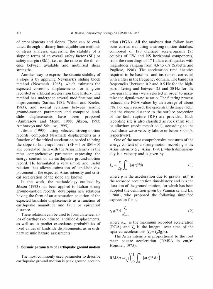
RMSA=0.14PGA (5) along the sliding surface. Therefore, even if areliable dynamic safety factor could be evaluated,where PGA and RMSA are expressed in cm/s2,this provides no information about the stabilityand the regression has an adjusted squared correla-conditions reached by the landslide mass after thetion coefficient of 0.81. More refined relations ofseismic shaking.IA and RMSA as a function of PGA invoking a

Moreover, pseudostatic approaches, incorpo-power law correlation are shown in Fig. 1. Theserating PGA for seismic stability analyses, generallyallow simple estimates of IA or, alternatively,underestimate the safety factor of the slope. AnRMSA for a given value of PGA.effective acceleration (such as RMSA) could bebetter assumed as representative of a pulse ofconstant acceleration with a rectangular shape3. Dynamic stability analysisacting for the entire strong-motion duration.

Newmark’s method overcomes these problemsSeismic forces acting on a slope induce accelera-tions, whose direction and magnitude vary at any by computing the cumulative coseismic displace-

Fig. 1. Relationships among Arias intensity, root mean square acceleration and peak ground acceleration (Italian strong-motiondatabase).


ment of the landslide mass taking into account general failure of the landslide mass may occur.The critical displacement depends on the rheologi-strong-motion duration, frequency content, and

stochastic variability of the seismic motion of the cal behavior of the landslide mass. Masses thatdisplay a brittle behavior (i.e., coherent andentire acceleration time history.

The required input to perform a Newmark disrupted slides, and falls) have a lower criticaldisplacement than masses whose ductility accom-analysis are a digitized acceleration time history

and the critical acceleration needed to reach the modates greater deformations prior to sliding (i.e.,lateral spreads and flows). In this study, failureslimit equilibrium (SF=1 or SM=0).

The common assumptions and limitations occurring in rocky slopes (disrupted falls andslides) have been assimilated to the first category,involved in Newmark’s method are:

1. the sliding mass is assumed to be a rigid- for which a critical displacement of 5 cm(Wieczorek et al., 1985) has been assumed, whileplastic body;

2. no permanent displacements are allowed for a critical displacement of 10 cm has been assumedfor flows and slides occurring in cohesive soilsaccelerations below the critical acceleration;

3. plastic deformations on the sliding surface are (Jibson and Keefer, 1993).After the earthquake, for those landslidesallowed when the critical acceleration is

exceeded; exceeding the critical displacement, a static analysiswith residual shear strengths can be performed to4. the critical acceleration is not strain-dependent;

5. static and dynamic strengths are considered to evaluate post-seismic safety conditions (Jibson andKeefer, 1993). Two cases arise:be the same and constant;

6. no pore-water pressure increment is considered. 1. the static safety factor in residual strength con-ditions is less than 1, or the correspondingAnyway, some of these assumptions can be

removed by the analyst. safety margin is less than 0: the slope is notstable and undergoes a general failure;The last two assumptions can represent limita-

tions too restrictive to perform a reliable displace- 2. the static safety factor in residual strength con-ditions is greater than 1 or the correspondingments analysis. In fact, strain-softening soils can

undergo large shear-strength degradation under safety margin is greater than 0: the slope isstable and deformation will cease after the endcyclic strain; shear strengths, after reaching peak

values, suddenly decrease toward residual values. of the seismic shaking. However, the final dis-placement will range from the displacementAgain, residual shear strengths imply lower values

for the critical acceleration, increasing the cumula- computed with peak shear strengths (maximumvalue of the critical acceleration) to the displace-tive displacement reached by the landslide mass

after the seismic shaking. Thus, performing a ment computed with residual shear strengths(minimum value of the critical acceleration).Newmark analysis assuming peak shear strengths

could underestimate the final coseismic displace- The latter allows the upper bound of theexpected displacements to be estimated andments. On the contrary, rate effects on shear

strength parameters due to fast shearing, strain- overcomes the problem of considering criticalacceleration to be strain-independent.hardening materials, and soils that display a vis-

coplastic response due to dynamic pore-pressure In saturated soils, the pore-water pressure canrise due to transient loads; in loose soils, the watereffects (Jibson and Harp, 1996), can actually pro-

duce an overestimation of the coseismic displace- pressure can balance the effective stress causingthe soil to liquefy (cyclic or dynamic liquefaction).ments when Newmark’s methodology is applied.

The stability conditions after the earthquake In dense soils, water pressure results in an increaseof the shear strengths during the cyclic loadingshaking can be assessed in terms of critical dis-

placement. Critical displacement is defined as the due to dilation; this will increase the short-termstability conditions of the slope. After the earth-coseismic displacement beyond which ground

cracking is produced, shear strengths along the quake, however, the shear strengths decrease dueto the generation of positive pore pressures, andsliding surface approach residual values, and a


thus the long-term stability conditions of the slope of pore-pressure generation (Martin and Seed,become worse than the short-term stability condi- 1978) or through simplified procedures (Matsuitions. This mechanism explains the delay of hours et al., 1980).and even days between seismic shaking and sig- The critical acceleration coefficient is given by:nificant landslide movements in overconsolidatedclays and dense sands. Kc=(SF−1) sin b (7)

To determine the critical acceleration, conven-tional stability analyses to compute the static safety if Kc is acting parallel to the slope and by:factor of the slope are generally performed. InFig. 2, an infinite slope and a rotational slide are Kc=(SF−1) tan b (8)pictured to show the different significance of theslope/thrust angle, b (Newmark, 1965). The criti- if Kc is acting horizontally.cal acceleration coefficient, Kc, acting parallel to Strictly speaking, critical acceleration should bethe slope is given by the critical acceleration nor- defined in direction parallel to the sliding surfacemalized to acceleration of gravity. along which the landslide mass moves downslope.

For the simplest model of an infinite slope with However, for practical purposes, the analysis isa steady seepage parallel to slope, the static safety often simplified by taking into account horizontalfactor is given by (Lambe and Whitman, 1979): acceleration and neglecting the vertical component

of the ground motion, which contributes little tothe instability conditions. In the following, criticalacceleration is always referred to Kc, unless aSF=

c∞

cz

1

cos b+(1−ru) cos b tan w∞

sin b(6)

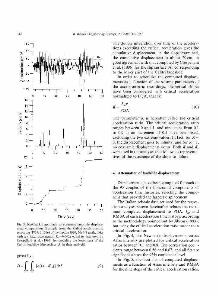
different definition is explicitly given.As an illustration of Newmark’s method, Fig. 3where z is the depth of the sliding surface from

shows the coseismic displacement computed forthe ground level, ru is the pore pressure coefficientthe lower part of the Calitri landslide (Hutchinson(Bishop, 1954), and c∞ and w∞ are the effectiveand Del Prete, 1985; Crespellani et al., 1996)shear-strength parameters. The relation overcomestriggered by the Irpinia 1980, Ms 6.8 earthquakethe problem of performing a stability calculation(Bernard and Zollo, 1989). When accelerationsin terms of total stresses. In fact, dynamic stabilityexceed the critical acceleration, the relative velocityanalyses are commonly carried out implementingbetween the block and its base increases until thethe undrained shear strength of the soil, although,acceleration drops below the threshold accelera-strictly, an effective stress analysis should be per-tion. The cumulative displacement continues toformed, taking into account the proper value ofincrease owing to inertial forces, and stops whenpore-water pressure developed during the cyclicthe velocity becomes zero.loading. The proper ru value under undrained

loading can be evaluated through rigorous analyses The resulting cumulative displacement is then

Fig. 2. Infinite slope ( left) and rotational slide (right). Kc refers to tangential critical acceleration; b is the slope angle (infinite slope)or the thrust angle (rotational slide).


The double integration over time of the accelera-tions exceeding the critical acceleration gives thecumulative displacement; in the slope examined,the cumulative displacement is about 20 cm, ingood agreement with that computed by Crespellaniet al. (1996) for the slip surface ‘A’, correspondingto the lower part of the Calitri landslide.

In order to generalize the computed displace-ments as a function of the seismic parameters ofthe accelerometric recordings, theoretical slopeshave been considered with critical accelerationnormalized to PGA, that is:

K=Kcg

PGA. (10)

The parameter K is hereafter called the criticalacceleration ratio. The critical acceleration ratioranges between 0 and 1, and nine steps from 0.1to 0.9 at an increment of 0.1 have been fixed,excluding the two extreme values. In fact, for K=0, the displacement goes to infinity, and for K=1,no coseismic displacements occur. Both K and Kcwere used in the analyses that follow, as representa-tives of the resistance of the slope to failure.

4. Attenuation of landslide displacement

Displacements have been computed for each ofthe 95 couples of the horizontal components ofacceleration time histories, selecting the compo-nent that provided the largest displacement.

The Italian seismic data set used for the regres-sion analyses shown hereinafter relates the maxi-mum computed displacement to PGA, IA, andRMSA of each acceleration time history, accordingto the methodology pointed out by Jibson (1993),

Fig. 3. Newmark’s approach to coseismic landslide displace- but using the critical acceleration ratio rather thanment computation. Example from the Calitri accelerometric

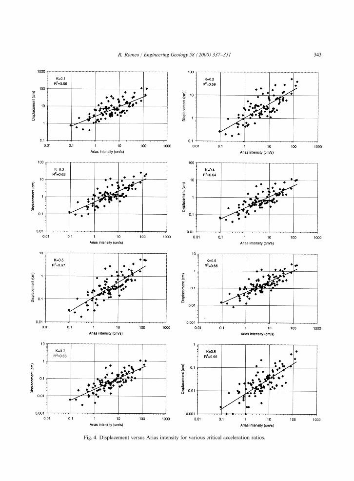
critical acceleration.recording (PGA 0.156g) of the Irpinia 1980, Ms 6.8 earthquakeIn Fig. 4, the Newmark displacements versuswith a critical acceleration Kc=0.045g equal to that used by

Crespellani et al. (1996) for modeling the lower part of the Arias intensity are plotted for critical accelerationCalitri landslide (slip surface ‘A’ in their analysis). ratios between 0.1 and 0.8. The correlation coeffi-

cients range between 0.56 and 0.67, and all fits aresignificant above the 95% confidence level.given by:

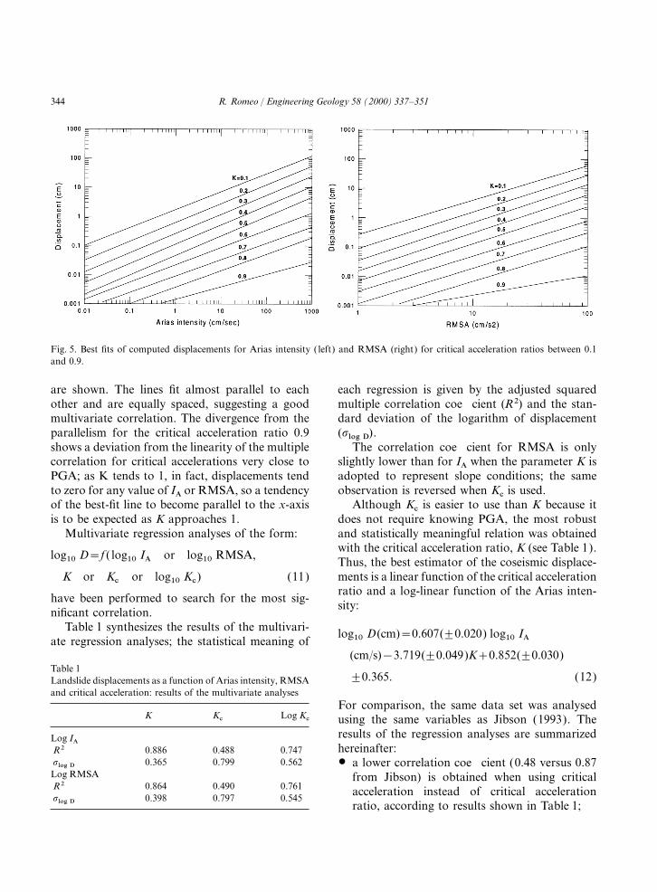
In Fig. 5, the best fits of computed displace-ments as a function of Arias intensity and RMSAD=P

0

t P0

t[a(t)−Kcg] dt2. (9)

for the nine steps of the critical acceleration ratios,


Fig. 4. Displacement versus Arias intensity for various critical acceleration ratios.


Fig. 5. Best fits of computed displacements for Arias intensity ( left) and RMSA (right) for critical acceleration ratios between 0.1and 0.9.

are shown. The lines fit almost parallel to each each regression is given by the adjusted squaredmultiple correlation coefficient (R2) and the stan-other and are equally spaced, suggesting a good

multivariate correlation. The divergence from the dard deviation of the logarithm of displacement(slog D).parallelism for the critical acceleration ratio 0.9

shows a deviation from the linearity of the multiple The correlation coefficient for RMSA is onlyslightly lower than for IA when the parameter K iscorrelation for critical accelerations very close to

PGA; as K tends to 1, in fact, displacements tend adopted to represent slope conditions; the sameobservation is reversed when Kc is used.to zero for any value of IA or RMSA, so a tendency

of the best-fit line to become parallel to the x-axis Although Kc is easier to use than K because itdoes not require knowing PGA, the most robustis to be expected as K approaches 1.

Multivariate regression analyses of the form: and statistically meaningful relation was obtainedwith the critical acceleration ratio, K (see Table 1).

log10

D=f ( log10

IA or log10

RMSA,Thus, the best estimator of the coseismic displace-ments is a linear function of the critical accelerationK or Kc or log

10Kc) (11)

ratio and a log-linear function of the Arias inten-have been performed to search for the most sig-

sity:nificant correlation.

Table 1 synthesizes the results of the multivari- log10

D(cm)=0.607(±0.020) log10

IAate regression analyses; the statistical meaning of(cm/s)−3.719(±0.049)K+0.852(±0.030)

Table 1±0.365. (12)Landslide displacements as a function of Arias intensity, RMSA

and critical acceleration: results of the multivariate analysesFor comparison, the same data set was analysed

K Kc Log Kc using the same variables as Jibson (1993). Theresults of the regression analyses are summarizedLog IA hereinafter:R2 0.886 0.488 0.747

slog D 0.365 0.799 0.562 $ a lower correlation coefficient (0.48 versus 0.87Log RMSA from Jibson) is obtained when using criticalR2 0.864 0.490 0.761 acceleration instead of critical accelerationslog D 0.398 0.797 0.545

ratio, according to results shown in Table 1;


$ the coefficient of log IA is almost the same as in turn, on shear strengths, geometric configurationand hydraulic conditions). Term S only accountsJibson (1.414 versus 1.460), while the coefficient

of the critical acceleration is higher (16.781 for the amplification of ground motion in soilscompared to that which is observed in rock orversus 6.642).

In conclusion, both Italian seismic data and the stiff soils.Coefficients a, b, c, e, f, and g are computeddifferent form of the critical acceleration are

responsible for the differences between the Jibson through a linear multivariate analysis, whilecoefficient d is calculated through a non-linearanalysis and the present analysis.

Since the Arias intensity depends on the earth- regression analysis and accounts for a fictitiousfocal depth. The term of anelastic attenuation, g,quake magnitude, the source-to-site distance, and

the geologic site conditions, IA has been expressed has been always found to be statistically meaning-less and very close to zero. The results of thein terms of these variables:regression analyses are reported in Table 2.

IA=f (M, R, S) then D=f (M, R, S, K ). (13)The predictive models are expressed in terms of

attenuation relations of the expected landslideAccording to Sabetta and Pugliese (1996), the bestattenuation function of the landslide displacements displacements for both rock and soil slopes as a

function of epicentral or fault distances:fitting Italian strong-motion data is:

log10

D=a+bM+c log10 log

10D (cm)=−1.144+0.591M−0.852 log

10×ER2+d2+eK+fS+gR±s (14) ×ERF2+2.62−3.703K+0.246S±0.403 (15)

where M refers to local magnitude for M≤5.5 andlog

10D (cm)=−1.281+0.648M−0.934 log

10to surface waves magnitude for M>5.5, to ensurethe best correlation as possible with moment mag- ×ERE2+3.52−3.699K+0.225S±0.418. (16)nitude (Hanks and Kanamori, 1979); R takes inturn the meaning of epicentral distance (RE) or The usefulness of such relations lies on the simple

estimation of the expected magnitude and source–the closest distance from the surface projection ofthe fault rupture (RF); and S has weight 0 for site distance for a reference earthquake (seismic

scenario) to predict landslide displacements, asrock or stiff soils and 1 for soft soils (shear wavevelocity not greater than 400 m/s and depth less well as on the possibility to perform probabilis-

tically based hazard analyses of expected landslidethan 20 m). The term S does not state that soilslopes can undergo greater displacements than displacements.

Fig. 6 illustrates the results of a parametricrock slopes, since they only depend on the criticalacceleration coefficient of the slope (depending, in analysis carried out to investigate the influence

Table 2Attenuation of landslide displacements as a function of magnitude, distance, local site conditions and critical acceleration ratio:results of the multivariate regression analyses

Coefficients Log D=f(M, log RF, K, S) Log D=f(M, log RE, K, S)

a −1.144±0.125 −1.281± 0.134b 0.591±0.026 0.648±0.030c −0.852±0.041 −0.934±0.051d 2.6 3.5e −3.703±0.055 −3.699±0.057f 0.246±0.028 0.225±0.029g 0.0 0.0R2 0.861 0.851slog D 0.403 0.418


Fig. 6. Graphical illustration of the influence exerted by parameters of Eqs. (15) and (16) on the expected landslide displacements.The ‘reference’ curve has been drawn for an M6 earthquake, epicentral distances [Eq. (16)], a critical acceleration ratio of 0.1, arock slope (S=0), and median values of computed displacements (slog D=0). Curve ‘fault’ has the same parameters of the ‘reference’but has been drawn using Eq. (15) (fault distance instead of epicentral distance). Curve ‘sigma’ has been plotted adding uncertaintyin the computed displacements (slog D=1). Curve ‘soil’ displays the attenuation of the landslide displacements for soil slopes (S=1)instead of rock slopes. Finally, the ‘K0.2’ curve has been drawn for a critical acceleration ratio twice the ‘reference’ one. Solid lines‘10 cm’ and ‘5 cm’ show critical displacements for flows and disrupted slides, respectively.

exerted by the parameters of Eqs. (15) and (16). the uncertainty (slog D) in the expected landslidedisplacements is considered, displacements that areComparisons are made with regard to a ‘reference’a factor of 2.6 greater than the median displace-curve whose parameters are: M6 earthquake, epi-ments are predicted (curve ‘sigma’ in Fig. 6). Thecentral distances, critical acceleration ratio 0.1,term ‘S’ exerts an influence that is about two-rock slopes (S=0), and median values of computedthirds of that exerted by slog D, determining andisplacements (slog D=0).increment of about 70% in the expected landslideCritical displacements (Dc) for disrupted anddisplacements when taken into account. The samecoherent slides (5 cm) and for flows or slidesconsiderations can be argued for different referenceoccurring in slopes that behave as viscoplasticearthquakes, that is for different magnitude values.materials (10 cm) are also shown in Fig. 6. Curve

Eqs. (15) and (16) require the estimation of the‘fault’ refers to landslide displacements computedexpected PGA value. This can be easily done usingas a function of fault distance [Eq. (15)]. Thepublished attenuation relations of the peak groundsame displacement is computed at a greater dis-acceleration for Italy, such as those of Tento et al.tance by Eq. (16) than by Eq. (15), by a definition(1992), Romeo et al. (1996), Sabetta and Puglieseof epicentral distance (a 20% of increment, on(1996) and Rinaldis et al. (1998).average), up to a distance of about 100 km.

Nevertheless, fault distance attenuates less thanepicentral distance, as its c-coefficient [the distance 5. Discussion and applicationscoefficient in Eq. (15)] shows.

Coefficient ‘e’ of the critical acceleration ratio An immediate application of the methodologyproposed in this work is the formulation of anis practically the same in both equations. When


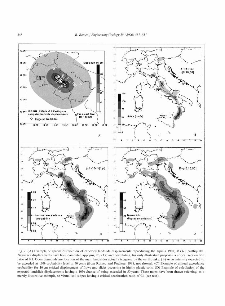
earthquake scenario in terms of expected landslide 1. Derivation of the expected landslide displace-displacements. As an example, the spatial distribu- ments through relation (12). Fig. 7B shows thetion of the expected landslide displacements repro- Arias intensity values expected to be exceededducing the Irpinia 1980, Ms 6.8 earthquake is at 10% probability level in 50 years (Romeoshown in Fig. 7A. The map is not slope-specific, and Pugliese, 1998)2; it allows computation ofthat is the computed displacements [through Eq. the expected landslide displacements [through(15)] are not referred to the actual critical accelera- Eq. (12)] at the same probability level (namely,tions of the slopes of the area; in fact, they have with an average return period of 475 years). Ofbeen calculated for virtual soil slopes with only course, landslide processes are not demon-one value of critical acceleration ratio (K=0.1). strated to follow stationary models of occur-In the same figure, the largest landslides triggered rence as for earthquakes, so this map must beby the Irpinia earthquake (D’Elia et al., 1985; interpreted with care. It shows only that soilCotecchia, 1986) are shown together with the fault slopes in the darkest area with a critical acceler-trace of the main rupture. Some landslides lie in ation ratio 0.1 or lower, for instance, couldthe area where this simple model predicts displace- experience coseismic displacements equal to orments between 10 and 25 cm; for these landslides, greater than 57 cm, with a 10% chance of beingtriggered at a large distance from the fault rupture, exceeded in the next 50 years.a critical acceleration ratio close to 0.1 was plausi-

2. Derivation of the expected landslide displace-ble when the earthquake occurred.

ments directly using relations (15) and (16).Some real cases, among the landslides triggeredFig. 7C and D shows two ways of expressingby the Irpinia earthquake, have been examined tothe potential landslide hazard assuming, as atest the validity of the proposed methodology, andmerely illustrative example, that soil slopes maythe results are summarized in Table 3, where, forbe characterized by a critical acceleration ratioeach landslide (column A), the type of movementof 0.1. Fig. 7C shows the annual probability(B), the closest distance from the fault rupture (C)exceeding the critical displacement of 10 cm,and the critical acceleration ratio (D), are reported.while in Fig. 7D, displacements that are expectedThe landslide displacements, computed throughto be exceeded at the 10% probability level inthe present methodology [Eq. (15), column G],50 years are depicted. Annual frequency prob-are then compared with those (F) reported inability maps, such as that in Fig. 7C, are usefulspecific studies (E). The results of the predictedto show the influence of frequent earthquakesdisplacements are in good agreement with theon the expected landslide displacements; on theactual observations of the behavior of the land-contrary, landslide hazard maps for long returnslides or with the dynamic analyses specifically

carried out. period, such as that in Fig. 7D, highlight theThe Paola earth flow was reactivated 10 days influence of less frequent and higher energy

after the main shock at a distance of 143 km from seismic events. In the simplistic assumptionsthe closest point of the main fault rupture. made for only illustrative purposes, Fig. 7B andAlthough intense rainfalls following the seismic 7D show that the maximum expected landslideevent were the main causes of the reactivation, an displacements are similar using Eq. (12) (49–important role was attributed to the earthquake 57 cm), and using Eq. (16) (50–60 cm). Thisin determining a shear strength reduction of the convergence facilitates two alternative but sim-materials involved in the landslide (Cotecchia, ilar ways to compute the expected displacements:1986). 1.1. estimate the PGA value for the proper

An alternative way to express the susceptibility magnitude–distance couple;of slopes to fail under seismic conditions is toperform a seismically induced landslide hazardanalysis. Two methodologies and applications 2 Seismic hazard maps of Italy are available at the following

web site: http://www.dstn.it/ssn/RT/rt9701/frameset.html.emerge from this study:


Fig. 7. (A) Example of spatial distribution of expected landslide displacements reproducing the Irpinia 1980, Ms 6.8 earthquake.Newmark displacements have been computed applying Eq. (15) and postulating, for only illustrative purposes, a critical accelerationratio of 0.1. Open diamonds are location of the main landslides actually triggered by the earthquake. (B) Arias intensity expected tobe exceeded at 10% probability level in 50 years (from Romeo and Pugliese, 1998, not shown). (C) Example of annual exceedanceprobability for 10 cm critical displacement of flows and slides occurring in highly plastic soils. (D) Example of calculation of theexpected landslide displacements having a 10% chance of being exceeded in 50 years. These maps have been drawn referring, as amerely illustrative example, to virtual soil slopes having a critical acceleration ratio of 0.1 (see text).


Tab

le3

Com

pari

son

betw

een

disp

lace

men

tsco

mpu

ted

thro

ugh

the

prop

osed

met

hodo

logy

and

disp

lace

men

tsob

serv

edor

calc

ulat

edin

site

-spe

cific

stud

ies

for

seve

rall

ands

lides

re-a

ctiv

ated

byth

eIr

pini

a19

80,

Ms

6.8

eart

hqua

ke

A.

Loc

alit

yB

.K

inem

atic

sof

C.

Clo

sest

dist

ance

D.

Cri

tica

lE

.C

itat

ion

ofth

est

udie

sF

.O

bser

ved

orca

lcul

ated

1G

.D

ispl

acem

ents

(cm

)w

here

the

the

land

slid

efr

omth

esu

rfac

eac

cele

rati

onsp

ecifi

cally

carr

ied

out

for

disp

lace

men

ts(c

m)

repo

rted

com

pute

dth

roug

hth

ela

ndsl

ide

proj

ecti

onof

rati

o,K

each

land

slid

ein

the

site

-spe

cific

pres

ent

met

hodo

logy

occu

rred

the

faul

t(k

m)

stud

ies

cite

din

colu

mn

Eap

plyi

ngE

q.(1

5)

Cal

itri

Rot

atio

nal

slid

e20

0.07

Hut

chin

son

and

551

56D

elP

rete

,19

85;

Cre

spel

lani

etal

.,19

96A

ndre

tta

Rot

atio

nal

and

170.

07–0

.15

D’E

lia,

1992

70–2

0165

–33

tran

slat

iona

lsl

ide

Buo

nin-

vent

reM

udsl

ide

30.

08C

otec

chia

etal

.,19

86b;

Gen

eral

colla

pse

174

Del

Pre

tean

dT

riso

rio

Liu

zzi,

1992

Sene

rchi

aM

udsl

ide

90.

06C

otec

chia

etal

.,19

86a

Gen

eral

colla

pse

118

Per

gola

Rot

atio

nal

slid

e9

0.16

Cot

ecch

iaet

al.,

1986

a$

3050

S.G

iorg

ioSl

ide

and

eart

h40

0.24

Dra

mis

etal

.,19

82G

roun

dcr

acks

7L

aM

olar

aflo

w


1.2. derive the expected IA value from the rela- I anticipate investigating other seismicitytion given in Fig. 1; parameters such as the destructiveness potential

1.3. compute the expected displacements (Uang and Bertero, 1988), which has been demon-through Eq. (12) at the specific K-value. strated to play a fundamental role in determining

2.1. the same step as 1.1; the structural response to strong shakings, as well2.2. compute the expected displacements as extending the concept of failure probability to

through Eq. (15) or Eq. (16) at the specific landslide occurrence and recurrence probabilitiesK-value. to provide a forecasting where large landslide

For example, a soil slope with critical acceleration displacements are more likely to occur.coefficient Kc=0.03g located 10 km from the epi-center of a M6 earthquake will experience a PGAvalue of about 0.3g (using Sabetta and Pugliese’s, Acknowledgements1996 attenuation law), corresponding to anexpected IA of 52.97 cm/s (Fig. 1). The expected

I wish to thank R. Jibson and D. Keeferdisplacement at the critical acceleration coefficient(USGS), J. Wasowski (CNR/CE.RI.S.T.), and aK=0.1 will be 33.6 cm from Eq. (12) applyingfourth anonymous reviewer, for their helpful com-methodology 1, versus 32 cm computed throughments and criticism, which improved very muchEq. (16) using methodology 2.the paper. Special thanks to Prof. A. PrestininziThe concept that the maps in Fig. 7A–D repre-(University of Urbino), who continuously encour-sent neither an actual earthquake-induced land-aged me to carry on this research.slide scenario nor a specific geographical

distribution of the landslide hazard must bestressed. The maps need, in fact, to be combined

Referenceswith the actual geographical distribution of criticalacceleration values and need to be represented ata detailed scale (regional or local ). Ambraseys, N.N., Menu, J.M., 1988. Earthquake-induced

ground displacements. Earthquake Engineering and Struc-tural Dynamics 16 (7), 985–1006.

Ambraseys, N.N., Srbulov, M., 1995. Earthquake induced dis-6. Conclusions placements of slopes. Soil Dynamics and Earthquake Engi-neering 14, 59–71.

A direct method to compute coseismic landslide Arias, A., 1970. A measure of earthquake intensity. SeismicDesign for Nuclear Power Plants. Massachussetts Institutedisplacements has been formulated. This couplesof Technology Press, Cambridge, MA, pp. 438–483.the simplicity of evaluating earthquake triggering

Bernard, P., Zollo, A., 1989. The Irpinia (Italy) earthquake:parameters with the susceptibility of slopes todetailed analysis of a complex normal faulting. Journal of

undergo failure when subjected to cyclic loading. Geophysical Research 94 (2), 1631–1647.Tests carried out on some real cases taken from Bishop, A.W., 1954. The use of pore pressure coefficient in

landslides triggered by an M6.8 earthquake that practice. Geotechnique 4, 148–152.Cotecchia, V., 1986. Ground deformations and slope instabilityoccurred in southern Italy in 1980 (Irpinia earth-

produced by the earthquake of 23 November 1980 in Cam-quake) confirmed the validity of the proposed Eqs.pania and Basilicata, Proceedings of the International Sym-(12), (15) and (16) for predicting seismicallyposium on Engineering Geology Problems in Seismic Areas,

induced landslide displacements. IAEG, April 13–19, 1986, Bari, Italy Vol. 5., 31–100.This method is also suitable for modeling earth- Cotecchia, V., Del Prete, M., Tafuni, N., 1986a. Effects of earth-

quake-induced landslide scenarios and landslide quake of 23rd November 1980 on pre-existing landslides inthe Senerchia area (southern Italy), Proceedings of thehazard when maps of expected landslide displace-International Symposium on Engineering Geology Prob-ments for various K-values (as in Fig. 7A, C andlems in Seismic Areas, IAEG, April 13–19, 1986, Bari, ItalyD) and maps showing the distribution of criticalVol. 4, 177–198.

acceleration values are overlapped (Wieczorek Cotecchia, V., Lenti, V., Salvemini, A., Spilotro, G., 1986b.et al., 1985; Luzi and Pergalani, 1996; Jibson et al., Reactivation of the large ‘Buoninventre’ slide by the Irpinia

earthquake of 23 November 1980, Proceedings of the1998; Miles and Hoxx, 1999).


International Symposium on Engineering Geology Prob- geologic map sheet). Soil Dynamics and Earthquake Engi-neering 15, 83–94.lems in Seismic Areas, IAEG, April 13–19, 1986, Bari, Italy

Martin, P.P., Seed, H.B., 1978. APOLLO: a computer programVol. 4, 217–253.for the analysis of pore pressure generation and dissipationCrespellani, T., Madiai, C., Maugeri, M., 1996. Analisi di stabi-in horizontal sand layers during cyclic or earthquake load-lita di un pendio in condizioni sismiche e post-sismiche. Rivi-ing. Report No. UCB/EERC-78/21. Earthquake Engineer-sta Italiana di Geotecnica, XXX (1), 50–61.ing Research Center, University of California, Berkeley, CA.D’Elia, B., Esu, F., Pellegrino, A., Pescatore, T.S., 1985. Some

Matsui, T., Ohara, H., Ito, T., 1980. Cyclic stress–strain historyeffects on natural slope stability induced by the 1980 Italianand shear characteristics of clay. Journal of Geotechnicalearthquake, Proceedings of the 11th ICSMFE, San Fran-Engineering Division, ASCE 106, GT10, 1101–1120.cisco, CA Vol. 4, 1943–1949.

Miles, S.B., Hoxx, C.L., 1999. Rigorous landslide hazard zona-D’Elia, B., 1992. Dynamic aspects of a landslide reactivated by

tion using Newmark’s method and stochastic groundthe November 32, 1980 Irpinia earthquake (southern Italy), motion simulation. Soil Dynamics and Earthquake Engi-Proceedings of the French–Italian Conference on Slope Sta- neering 18, 305–323.bility in Seismic Areas, May 14–15, 1992, Bordighera, Newmark, N.M., 1965. Effects of earthquakes on dams andItaly, 33–45. embankments. Geotechnique 15 (2), 139–159.

Del Prete, M., Trisorio Liuzzi, G., 1992. Reactivation of mud- Rinaldis, D., Berardi, R., Theodulikis, N., Margaris, B., 1998.slides after a long quiescent period the case of Buoninventre Empirical predictive models based on a joint Italian andin southern Apennines, Proceedings of the French–Italian Greek strong-motion database: I, peak ground accelerationConference on Slope Stability in Seismic Areas, May 14–15, and velocity. Proceedings of the 11th European Conference1992, Bordighera, Italy, 33–45. on Earthquake Engineering, September 6–11, 1997, CNIT,

Paris La Defense, France.Dramis, F., Prestininzi, A., Cognini, L., Genevois, R., Lom-Romeo, R., Tranfaglia, G., Castenetto, S., 1996. Engineering-bardi, S., 1982. Surface fractures connected with the south-

developed relations derived from the strongest instrumen-ern Italy earthquake (November 1980) — distribution andtally-detected Italian earthquakes. Proceedings of the 11thgeomorphological implications, Proceedings of the 4thWCEE, June 23–28, 1996, Acapulco, Mexico, Paper No.International Congress of IAEG, December 10–15, 1982,1466.New Delhi, India Vol. 8., 55–66.

Romeo, R., Delfino, L., 1997. Catalogo nazionale degli EffettiHanks, T.C., Kanamori, H., 1979. A moment magnitude scale.Deformativi del suolo Indotti da forti Terremoti. RapportoJournal of Geophysical Research 84, 2348–2350.Tecnico SSN/RT/97/04, Roma, Maggio 1997. 38 pp.Housner, G.W., 1975. Measures of severity of earthquake

Romeo, R., Pugliese, A., 1998. A global earthquake hazardground shaking, Proceedings of the US National Conference

assessment of Italy. Proceedings of the 11th European Con-on Earthquake Engineering, EERI, Ann Arbor, MI, June ference on Earthquake Engineering, September 6–11, 1997,1975, 25–33. CNIT, Paris La Defense, France.

Hutchinson, J.N., Del Prete, M., 1985. Landslides at Calitri, Sabetta, F., Pugliese, A., 1996. Estimation of response spectrasouthern Apennines, reactivated by the earthquake of 23rd and simulation of nonstationary earthquake ground motion.November 1980. Geologia Applicata e ldrogeologia XX Bulletin Seismological Society of America 86 (2), 337–352.(1), 9–38. Sarma, S.K., 1981. Seismic displacement analysis of earth dams.

Jibson, R.W., 1993. Predicting earthquake-induced landslide Journal of Geotechnical Engineering Division, ASCE 107displacement using Newmark’s sliding block analysis. (12), 1735–1739.Transportation Research Board, National Research Coun- Tento, A., Franceschina, L., Marcellini, A., 1992. Expected

ground motion evaluation for Italian sites, Proceedings ofcil, Washington D.C., TR record 1411, 9–17.the 10th WCEE, July 19–24, Madrid, 489–494.Jibson, R.W., Keefer, D.K., 1993. Analysis of the seismic origin

Uang, C., Bertero, V.V., 1988. Implications of recorded earth-of landslides examples from the New Madrid seismic zone.quake ground motions on seismic design of building struc-Geological Society of American Bulletin 105, 521–536.tures. Report No. UCB/EERC 88/13. EarthquakeJibson, R.W., Harp, E.L., 1996. The Springdale, Utah, land-Engineering Research Center, University of California,slide: an extraordinary event. Environmental and Engineer-Berkeley, CA.ing Geoscience 2 (2), 137–150.

Vanmarke, E.H., Lai, S.P., 1980. Strong-motion duration andJibson, R.W., Harp, E.L., Michael, J.A., 1998. A method forRMS amplitude of earthquake records. Bulletin Seismologi-

producing digital probabilistic seismic landslide hazardcal Society of America 70, 1293–1307.

maps: an example from the Los Angeles, California, area. Wieczorek, G.F., Wilson, R.C., Harp, E.L., 1985. Map showingUS Geological Survey Open-File Report 98-113. 17 pp., 2 pl slope stability during earthquakes in San Mateo County,

Keefer, D.K., 1984. Landslides caused by earthquakes. Geologi- California. Miscellaneous Investigation Maps I-1257-E,cal Society of American Bulletin 95, 406–421. U.S.G.S., 1985.

Lambe, T.W., Whitman, R.V., 1979. Soil Mechanics. Wiley, Wilson, R.C., Keefer, D.K., 1983. Dynamic analysis of a slopeNew York. 553 pp. failure from the 6 August 1979 Coyote Lake, California,

Luzi, L., Pergalani, F., 1996. Applications of statistical and GIS Earthquake. Bulletin Seismological Society of America 73(3), 863–877.techniques to slope instability zonation (1:50.000 Fabriano

Documents

Seismically induced landslide displacements: a predictive ...nceg.uop.edu.pk/workshop-17to31mar-05/Slides/day17/background... · Seismically induced landslide displacements: a predictive