Embed Size (px)
Citation preview
Seismic Tomography HS11S. Husen
Seismic TomographyFall semester 2011
8
66.5
7.5
01020304050607080
Dept
h (k
m)
0100
200300
400500
6000
1020304050607080
Dept
h (k
m) 500
600
6
6.5
6.5
7
7
7.5
7.5
8
88
2000
4000
Elev
. (m
)
2000
4000
Elev
. (m
)
1020304050607080
300200
100
01020304050607080
Dept
h (k
m
0
8 7
66.5
7.5
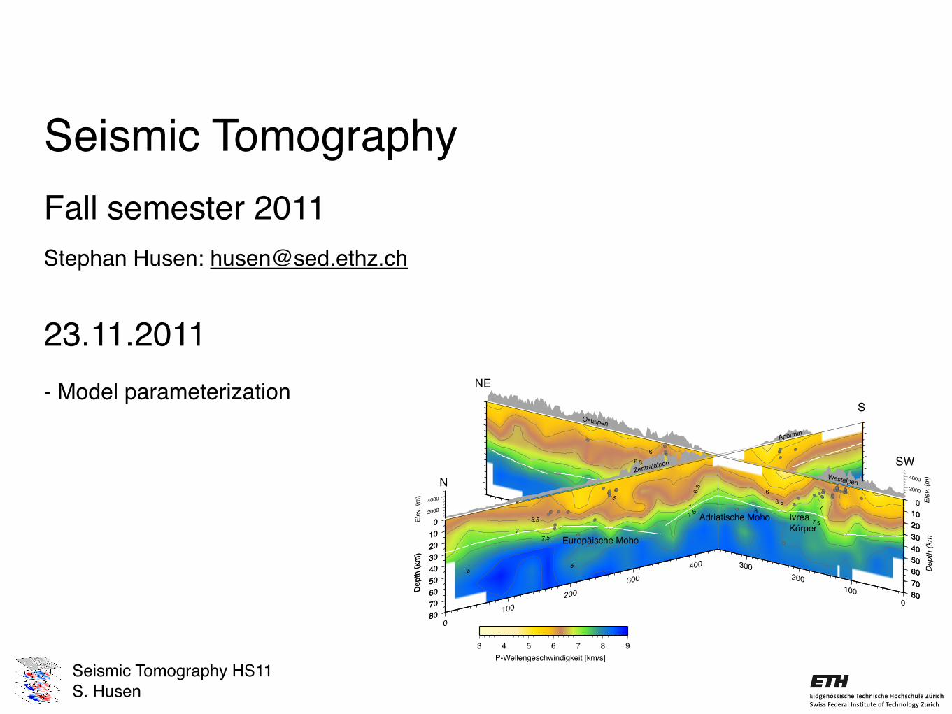
3 4 5 6 7 8 9P-Wellengeschwindigkeit [km/s]
N
S
SW
Ivrea Körper
Europäische Moho
Adriatische Moho
NE
Zentralalpen
Apennin
Westalpen
Ostalpen
Stephan Husen: [email protected]
23.11.2011- Model parameterization

Seismic Tomography HS11S. Husen
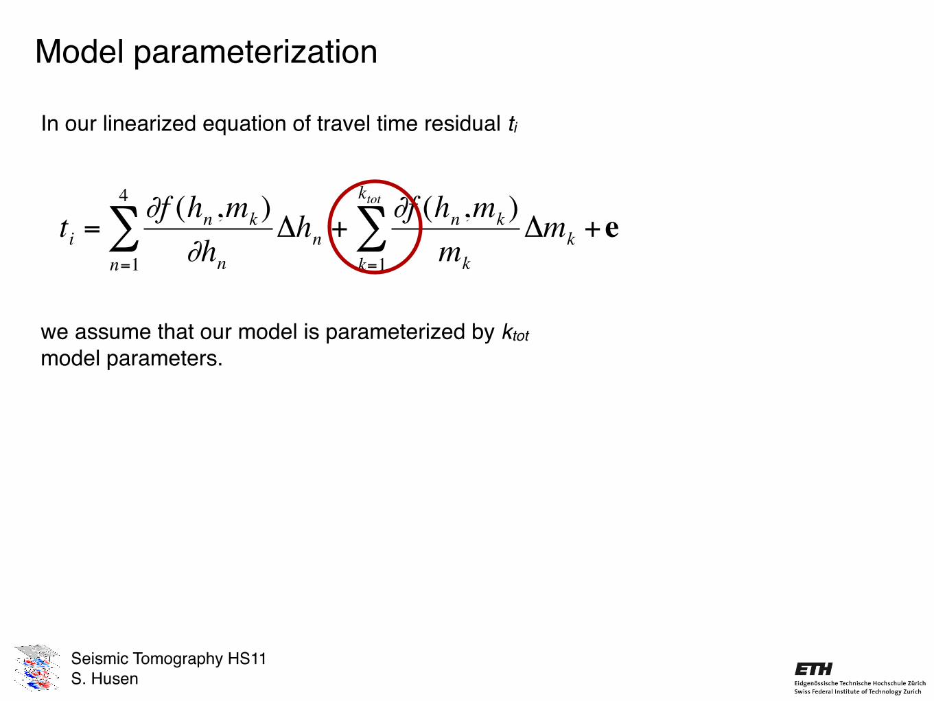
Model parameterization
€
ti =∂f (hn ,mk )
∂hnΔhn +
∂f (hn,mk )mk
Δmk +k=1
ktot
∑n=1
4
∑ e
In our linearized equation of travel time residual ti
we assume that our model is parameterized by ktot model parameters.
Seismic Tomography HS11S. Husen
Model parameterization
€
ti =∂f (hn ,mk )
∂hnΔhn +
∂f (hn,mk )mk
Δmk +k=1
ktot
∑n=1
4
∑ e
In our linearized equation of travel time residual ti
we assume that our model is parameterized by ktot model parameters.

Seismic Tomography HS11S. Husen
Model parameterization
€
ti =∂f (hn ,mk )
∂hnΔhn +
∂f (hn,mk )mk
Δmk +k=1
ktot
∑n=1
4
∑ e
In our linearized equation of travel time residual ti
we assume that our model is parameterized by ktot model parameters.
The (important) question is how do parameterize our model?
Seismic Tomography HS11S. Husen
Model parameterization
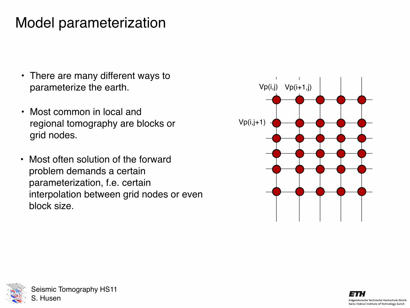
• There are many different ways to parameterize the earth.
• Most common in local and regional tomography are blocks or grid nodes.
• Most often solution of the forward problem demands a certain parameterization, f.e. certain interpolation between grid nodes or even block size.
Vp(i,j) Vp(i+1,j)
Vp(i,j+1)
Seismic Tomography HS11S. Husen
Model parameterization
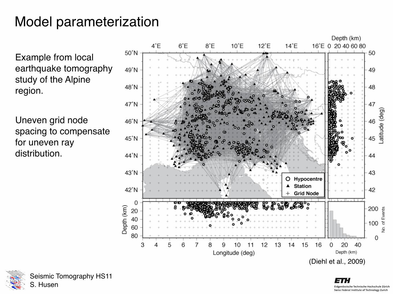
Example from local earthquake tomography study of the Alpine region.
Uneven grid node spacing to compensate for uneven ray distribution.
(Diehl et al., 2009)
Seismic Tomography HS11S. Husen
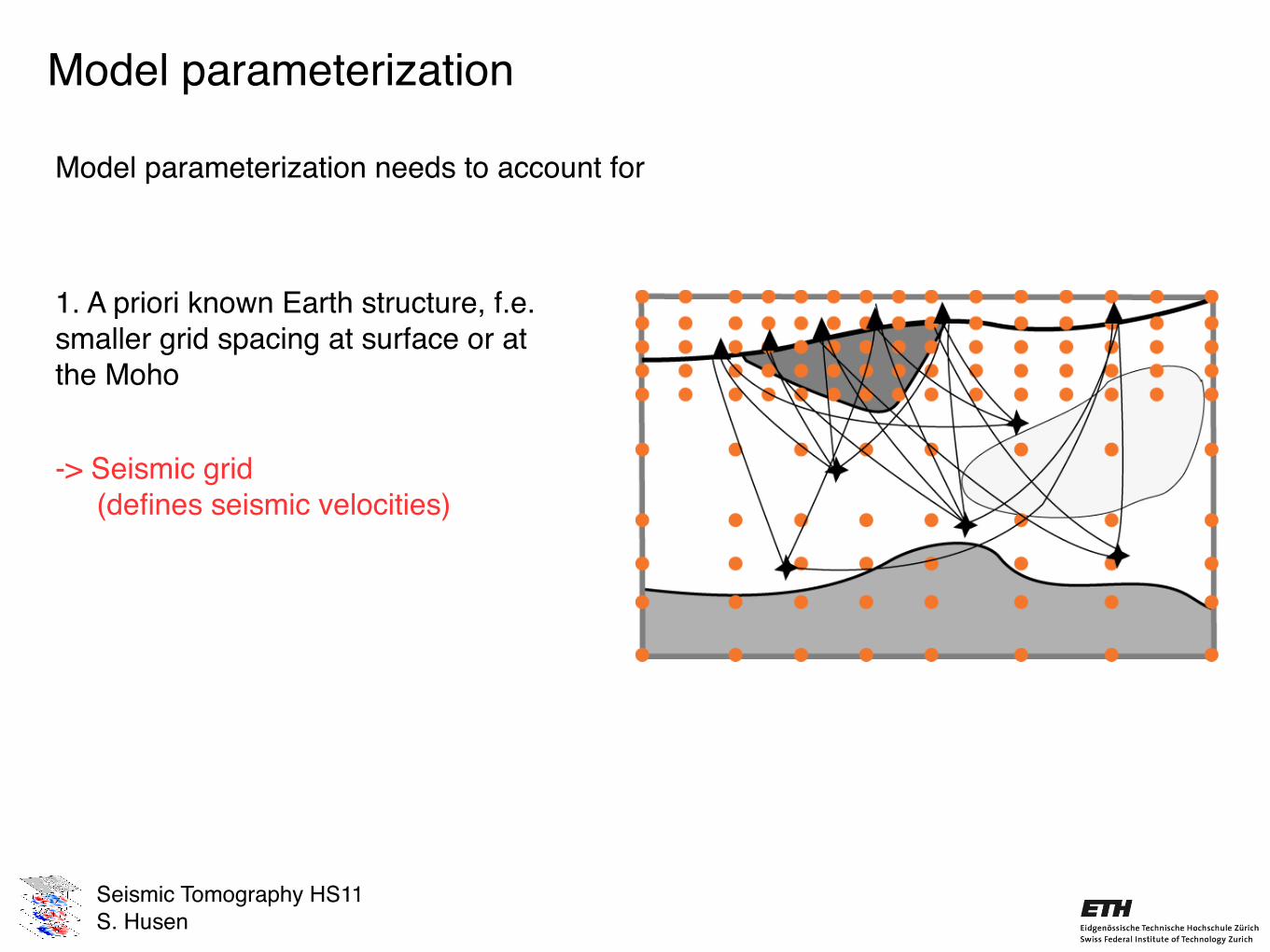
Model parameterization
Model parameterization needs to account for
1. A priori known Earth structure, f.e. smaller grid spacing at surface or at the Moho
-> Seismic grid (defines seismic velocities)
Seismic Tomography HS11S. Husen
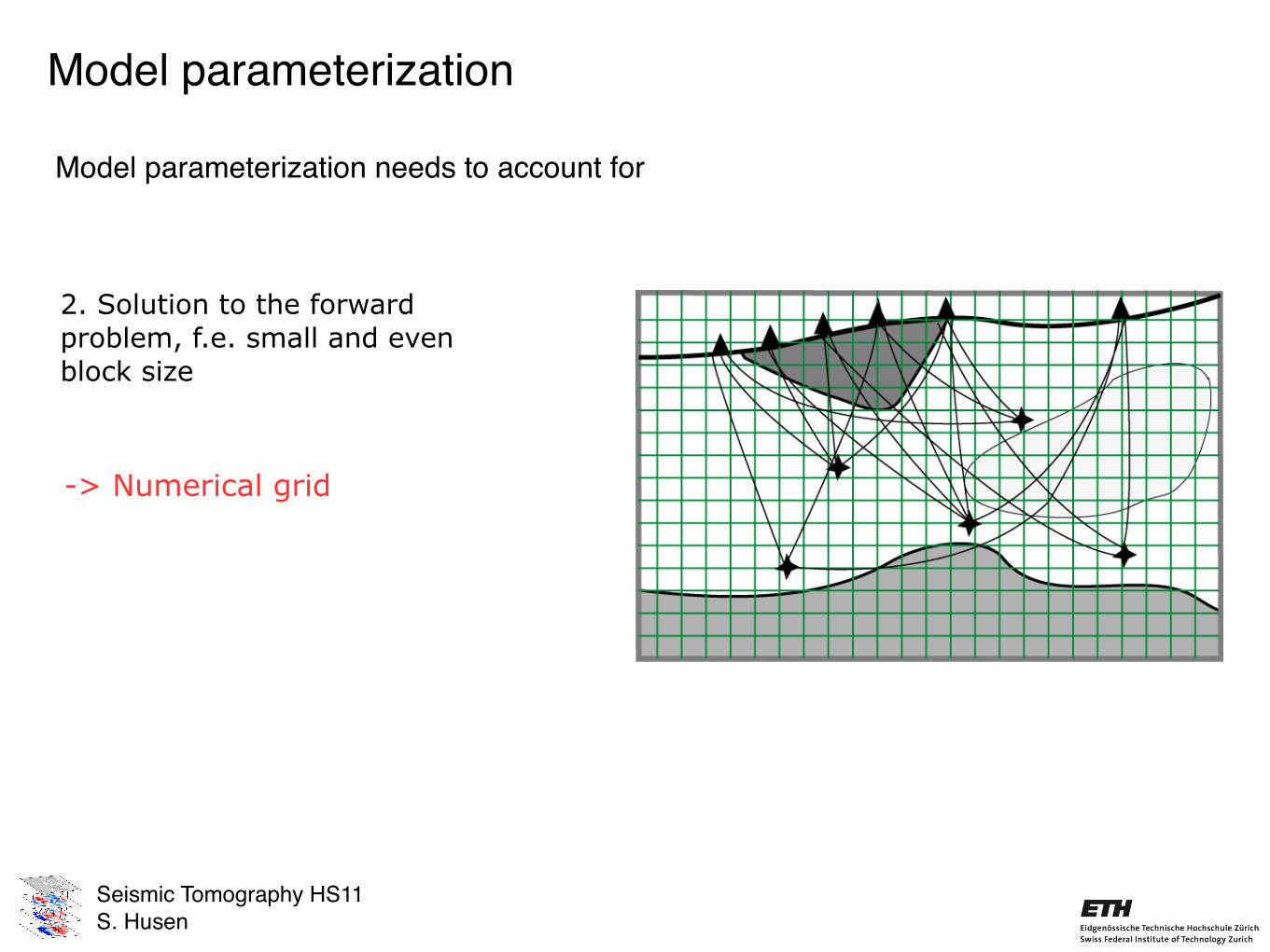
Model parameterization
2. Solution to the forward problem, f.e. small and even block size
-> Numerical grid
Model parameterization needs to account for
Seismic Tomography HS11S. Husen
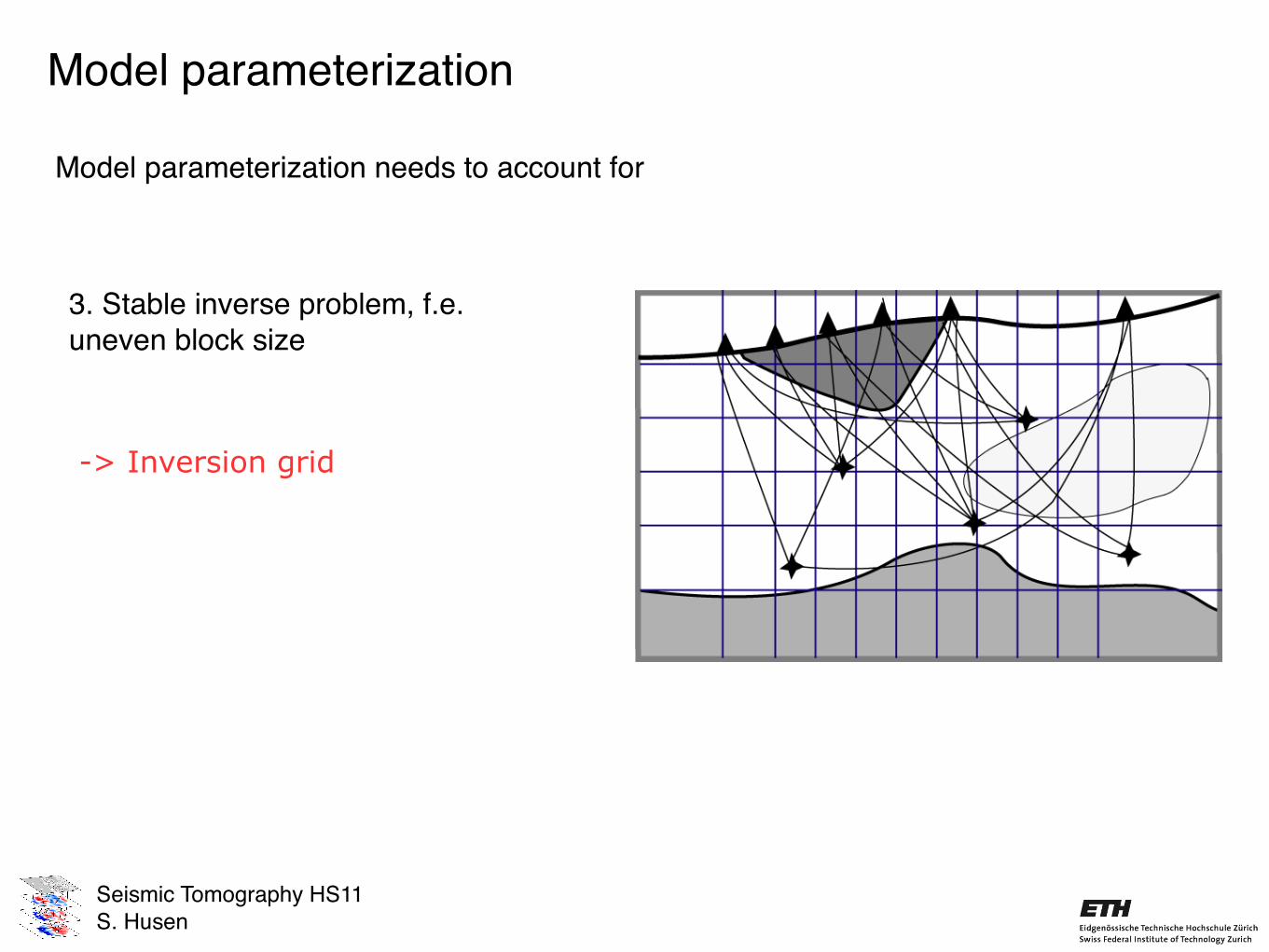
Model parameterization
Model parameterization needs to account for
3. Stable inverse problem, f.e. uneven block size
-> Inversion grid
Seismic Tomography HS11S. Husen
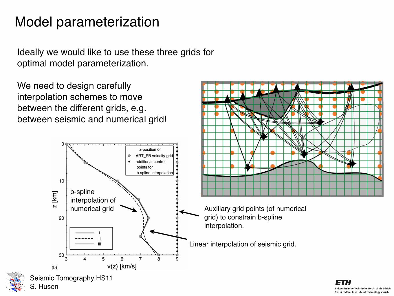
Model parameterization
Ideally we would like to use these three grids for optimal model parameterization.
We need to design carefully interpolation schemes to move between the different grids, e.g. between seismic and numerical grid!
F. Haslinger, E. Kissling / Physics of the Earth and Planetary Interiors 123 (2001) 103–114 105
Fig. 1. Example for inversion and velocity grids. (a) An uneven SIMULPS grid (full grey circles) defining the velocity model used for
ART PB ray tracing and inversion. Small black dots denote the even grid of control points used for RKP ray tracing. Velocity values
at control points are derived by linear interpolation on the uneven grid; (b) an example velocity-depth profile showing the effect of the
refined grid of control points. Velocity-depth functions: I used for ART PB ray tracing; II derived by cubic B-spline interpolation of the
ART PB grid velocities; III derived by cubic B-spline interpolation of the refined RKP grid.
Linear interpolation of seismic grid.
b-spline interpolation of numerical grid Auxiliary grid points (of numerical
grid) to constrain b-spline interpolation.
Seismic Tomography HS11S. Husen
Model parameterization
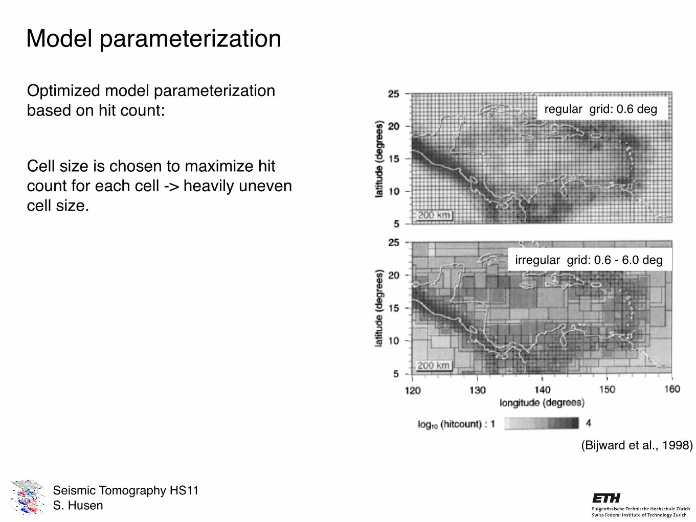
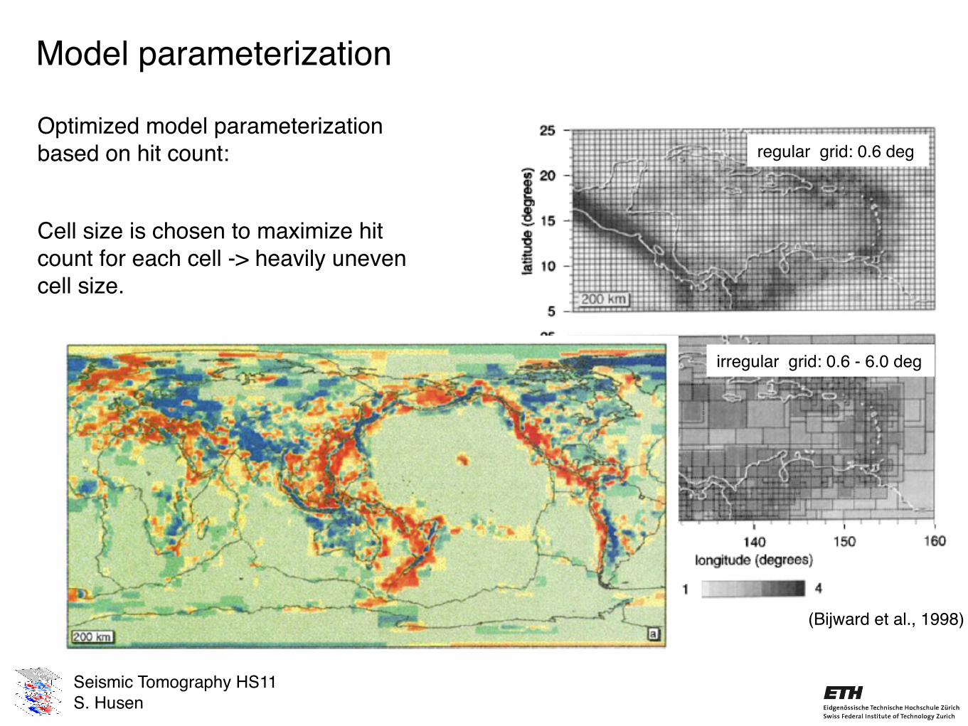
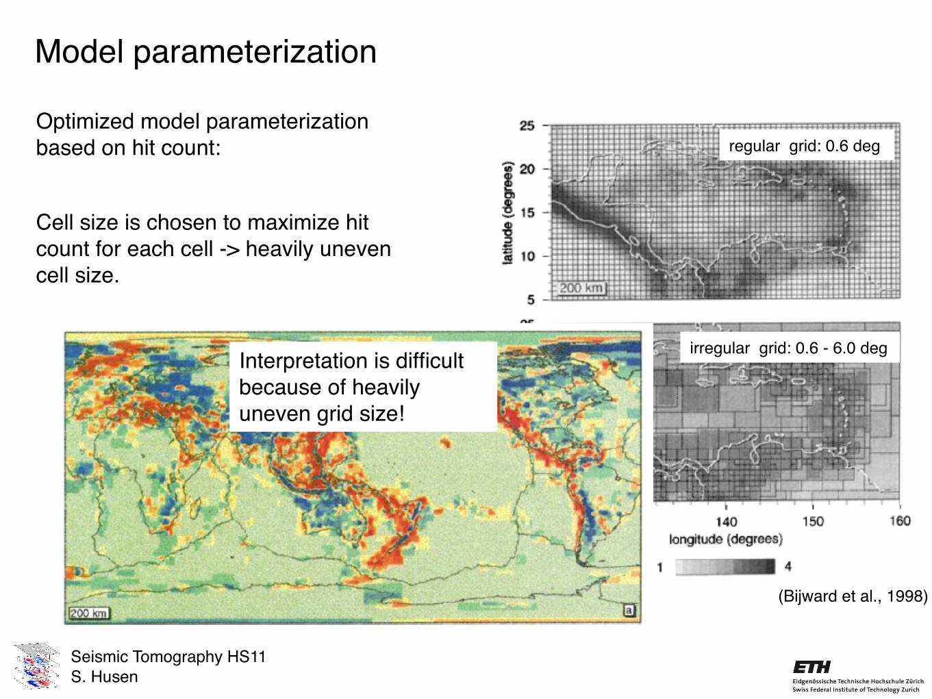
Optimized model parameterization based on hit count: regular grid: 0.6 deg
irregular grid: 0.6 - 6.0 deg
(Bijward et al., 1998)
Cell size is chosen to maximize hit count for each cell -> heavily uneven cell size.
Seismic Tomography HS11S. Husen
Model parameterization
Optimized model parameterization based on hit count: regular grid: 0.6 deg
irregular grid: 0.6 - 6.0 deg
(Bijward et al., 1998)
Cell size is chosen to maximize hit count for each cell -> heavily uneven cell size.
Seismic Tomography HS11S. Husen
Model parameterization
Optimized model parameterization based on hit count: regular grid: 0.6 deg
irregular grid: 0.6 - 6.0 deg
(Bijward et al., 1998)
Cell size is chosen to maximize hit count for each cell -> heavily uneven cell size.
Interpretation is difficult because of heavily uneven grid size!
Seismic Tomography HS11S. Husen
Model parameterization
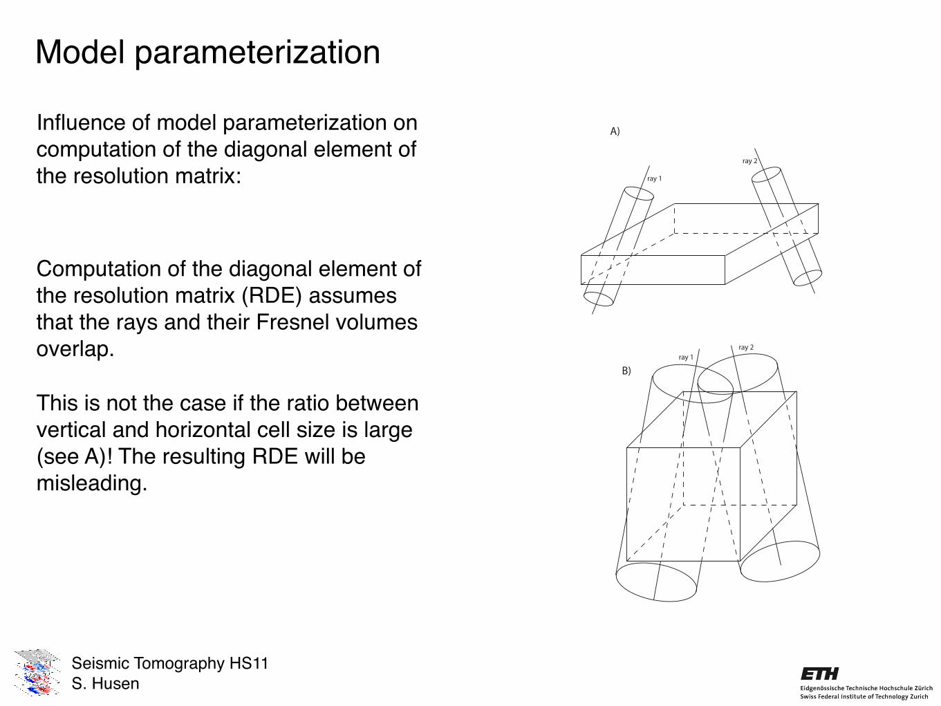
Influence of model parameterization on computation of the diagonal element of the resolution matrix:
Computation of the diagonal element of the resolution matrix (RDE) assumes that the rays and their Fresnel volumes overlap.
2 Principles of solution quality assessment in LET
uniform resolution in most areas in the studied volume.
Obviously, the model parametrization should be chosen to best represent ex-pected structure while allowing optimal resolution for study region. Optimal res-olution denotes as much as possible area with uniform resolution and uniformgridding. Wherever resolution or gridding shows strong lateral variations, the re-sulting image will be distorted (Kissling et al., 2001). To define the appropriategrid size for a tomography study, several parameters have to be taken into account.First of all, the horizontal size of the grid has to be larger than the wavelengthof the dominating frequency of picked wavelets. In the case of Costa Rica, thedominant frequency of the first arriving and interpreted wavelets is about 1Hz. Ifwe consider a P-wave travelling at 6km/s, the horizontal grid size should be morethan 6km. This is a theoretical limit. In practice, for regional studies, one wouldrarely go below 10km, because of insufficient data to cover each cell in the entirestudy region with enough rays. Moreover the proportions between the horizontaland the vertical size of the grid must be of the same order to allow reasonableresolution estimates. (see Figure 2.4).
Figure 2.4: Distortion of cells could lead to a wrong RDE value (for definition see section 2.3.1):A) RDE is calculated as if these two rays would cross within cell but the Fresnelvolumes do not overlap B) RDE is calculated as if these two rays would cross withincell but the Fresnel volumes overlap.
To avoid problems with incorrect resolution estimates, the ratio between thehorizontal and vertical cell size should net exceed a factor of 2.5, so that thereis more chance that the Fresnel volumes of crossing rays overlap. For a cell withhorizontal proportion of 10x10 km, the minimum vertical size is thus four kilome-tres. In addition to these concerns, we want to define an inversion grid that allowstreating an over-determined problem, where the number of unknowns is smallerthan the number of equations. Number of grid nodes added to the four location
26
This is not the case if the ratio between vertical and horizontal cell size is large (see A)! The resulting RDE will be misleading.
Seismic Tomography HS11S. Husen
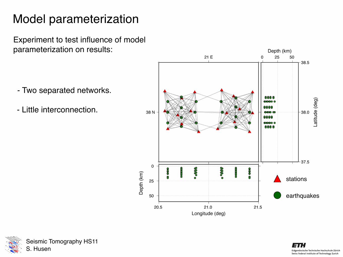
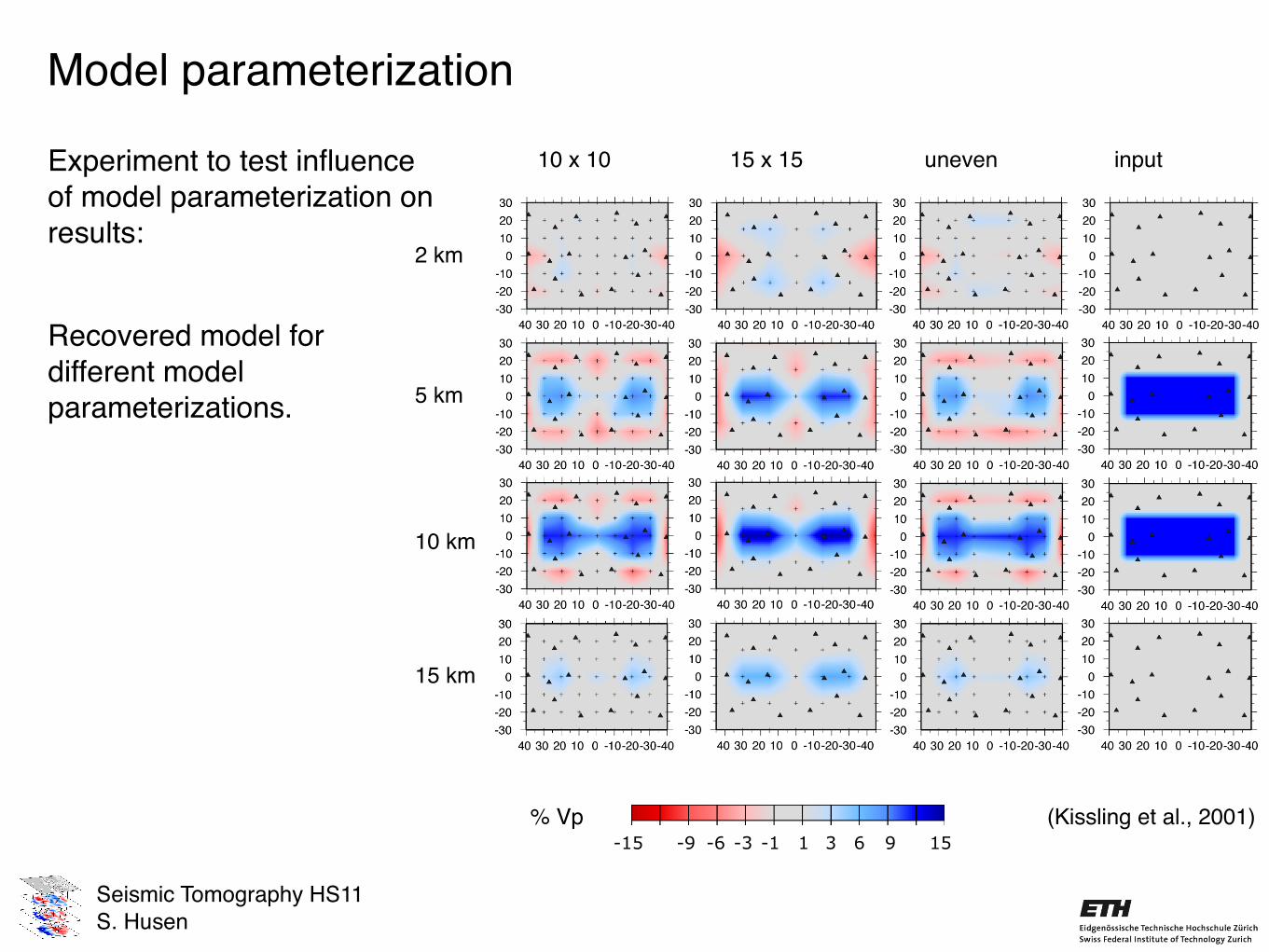
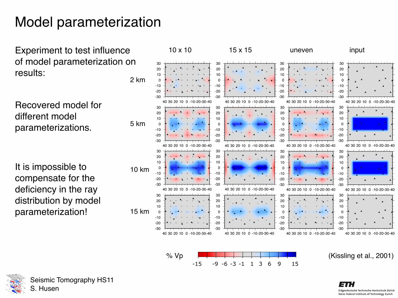
Model parameterizationExperiment to test influence of model parameterization on results:
- Two separated networks.
- Little interconnection.
stations
earthquakes
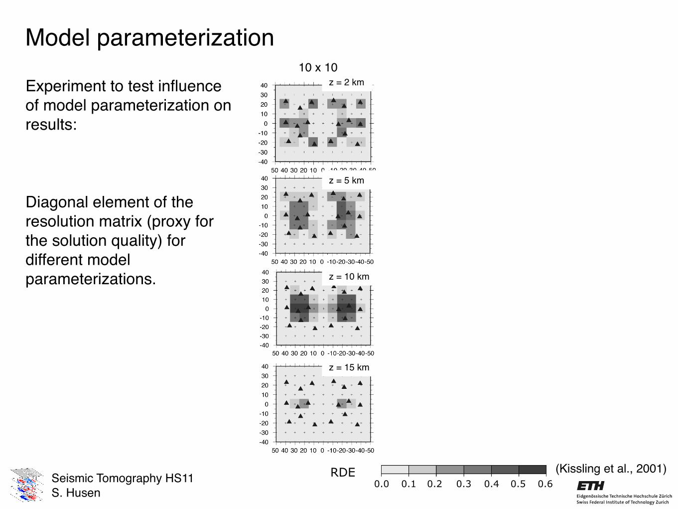
Seismic Tomography HS11S. Husen
Model parameterization
RDE0.0 0.1 0.2 0.3 0.4 0.5 0.6
10 x 10z = 2 km
z = 5 km
z = 10 km
z = 15 km
Experiment to test influence of model parameterization on results:
Diagonal element of the resolution matrix (proxy for the solution quality) for different model parameterizations.
(Kissling et al., 2001)
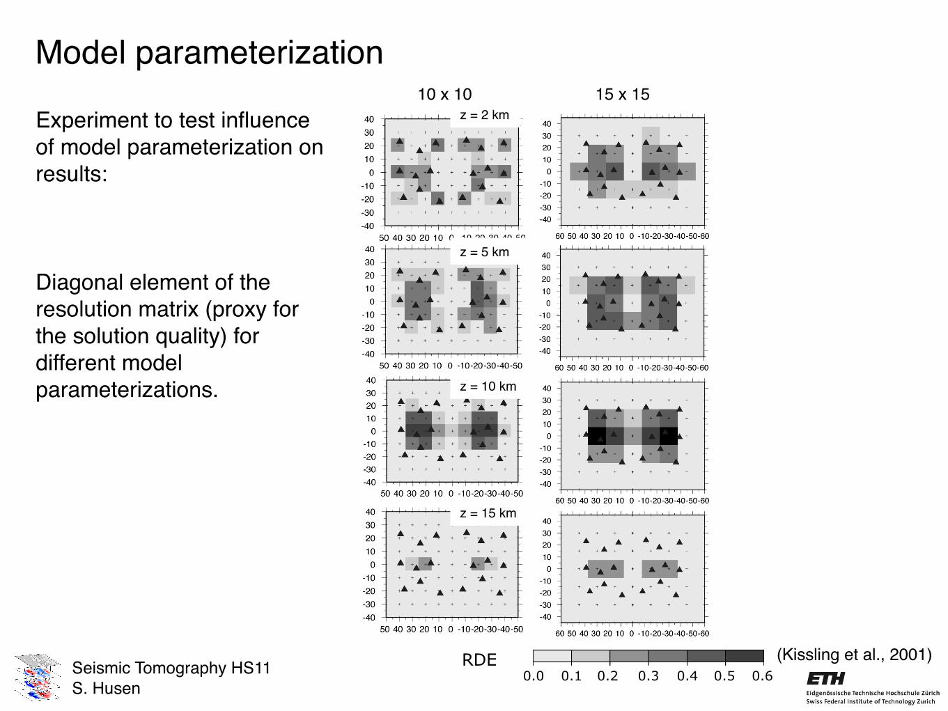
Seismic Tomography HS11S. Husen
Model parameterization
RDE0.0 0.1 0.2 0.3 0.4 0.5 0.6
10 x 10 15 x 15z = 2 km
z = 5 km
z = 10 km
z = 15 km
Experiment to test influence of model parameterization on results:
Diagonal element of the resolution matrix (proxy for the solution quality) for different model parameterizations.
(Kissling et al., 2001)
Seismic Tomography HS11S. Husen
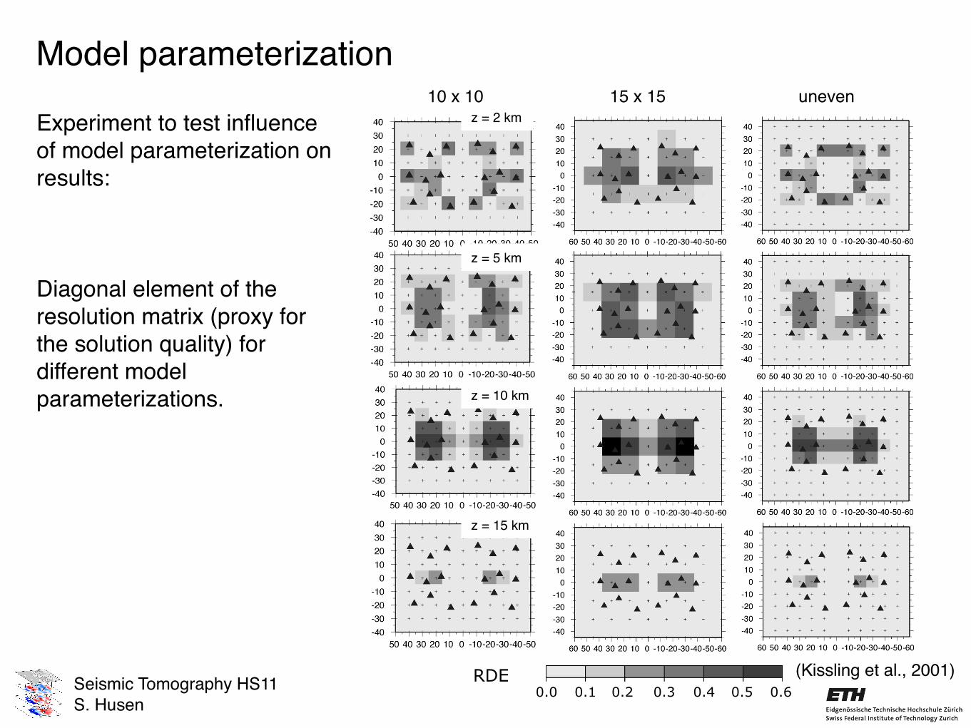
Model parameterization
RDE0.0 0.1 0.2 0.3 0.4 0.5 0.6
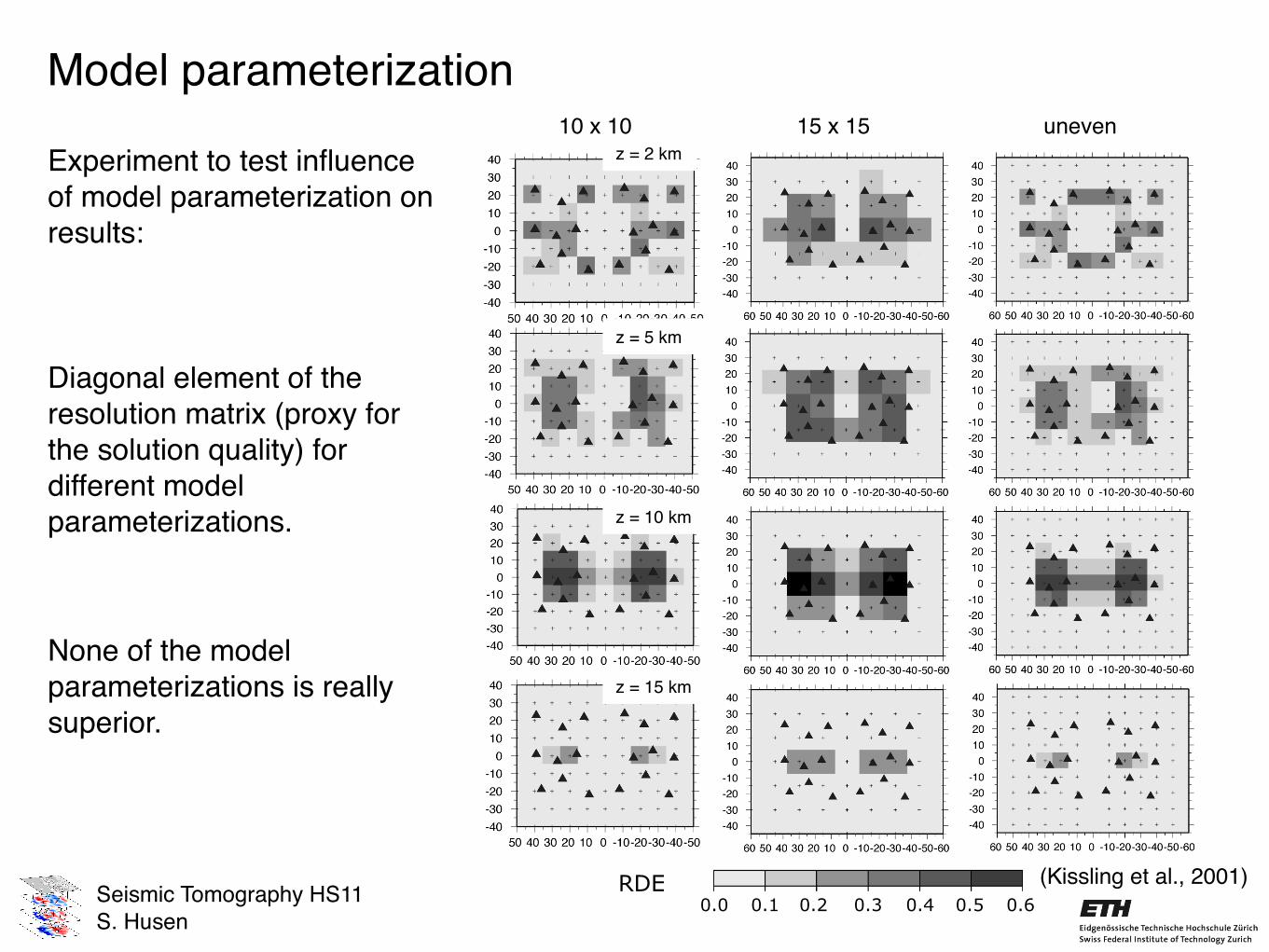
10 x 10 15 x 15 unevenz = 2 km
z = 5 km
z = 10 km
z = 15 km
Experiment to test influence of model parameterization on results:
Diagonal element of the resolution matrix (proxy for the solution quality) for different model parameterizations.
(Kissling et al., 2001)
Seismic Tomography HS11S. Husen
Model parameterization
RDE0.0 0.1 0.2 0.3 0.4 0.5 0.6
10 x 10 15 x 15 unevenz = 2 km
z = 5 km
z = 10 km
z = 15 km
Experiment to test influence of model parameterization on results:
Diagonal element of the resolution matrix (proxy for the solution quality) for different model parameterizations.
None of the model parameterizations is really superior.
(Kissling et al., 2001)
Seismic Tomography HS11S. Husen
Model parameterization
10 x 10
-15 -9 -3 3 9 15-1 1 6-6% Vp
2 km
5 km
10 km
15 km
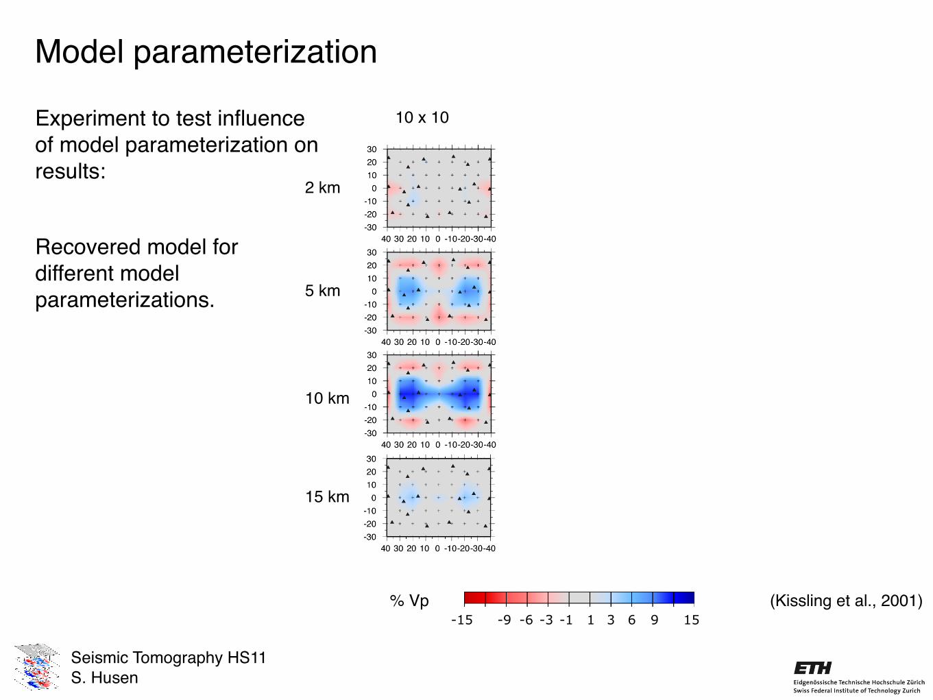
Experiment to test influence of model parameterization on results:
Recovered model for different model parameterizations.
(Kissling et al., 2001)
Seismic Tomography HS11S. Husen
Model parameterization
10 x 10 15 x 15
-15 -9 -3 3 9 15-1 1 6-6% Vp
2 km
5 km
10 km
15 km
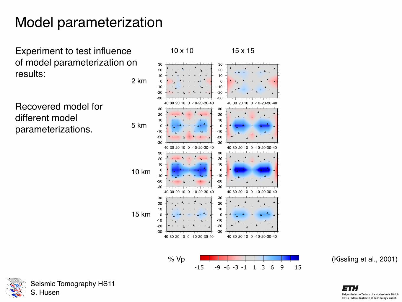
Experiment to test influence of model parameterization on results:
Recovered model for different model parameterizations.
(Kissling et al., 2001)
Seismic Tomography HS11S. Husen
Model parameterization
10 x 10 15 x 15 uneven
-15 -9 -3 3 9 15-1 1 6-6% Vp
2 km
5 km
10 km
15 km
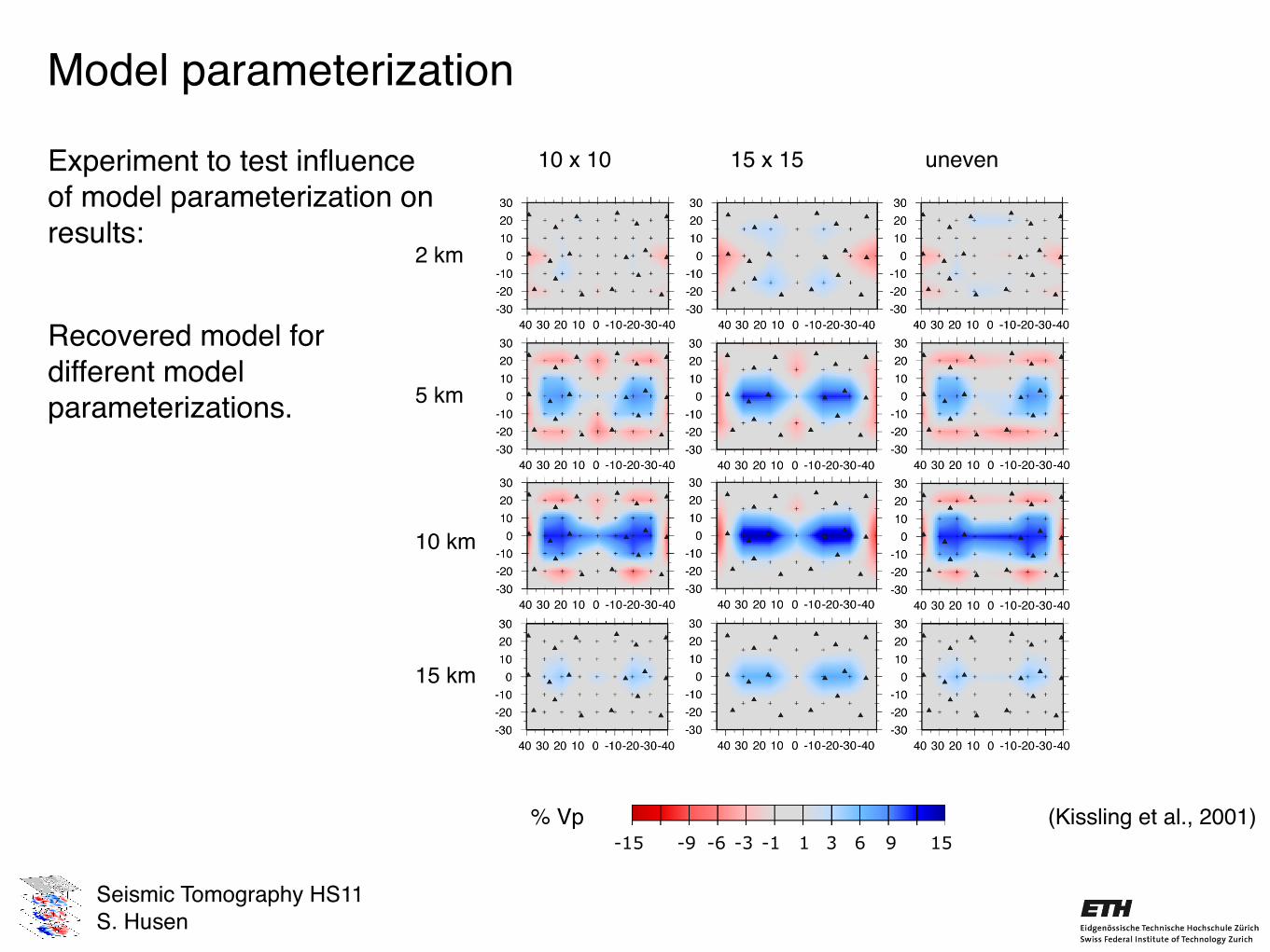
Experiment to test influence of model parameterization on results:
Recovered model for different model parameterizations.
(Kissling et al., 2001)
Seismic Tomography HS11S. Husen
Model parameterization
10 x 10 15 x 15 uneven
-15 -9 -3 3 9 15-1 1 6-6% Vp
2 km
5 km
10 km
15 km
inputExperiment to test influence of model parameterization on results:
Recovered model for different model parameterizations.
(Kissling et al., 2001)
Seismic Tomography HS11S. Husen
Model parameterization
10 x 10 15 x 15 uneven
-15 -9 -3 3 9 15-1 1 6-6% Vp
2 km
5 km
10 km
15 km
inputExperiment to test influence of model parameterization on results:
Recovered model for different model parameterizations.
It is impossible to compensate for the deficiency in the ray distribution by model parameterization!
(Kissling et al., 2001)
Seismic Tomography HS11S. Husen
Model parameterization
High-resolution 3-D P-wave model of the Alpine crust 1139
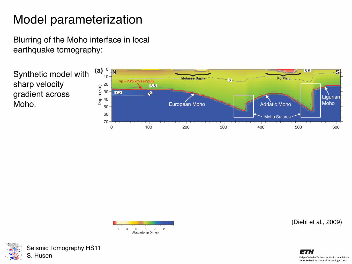
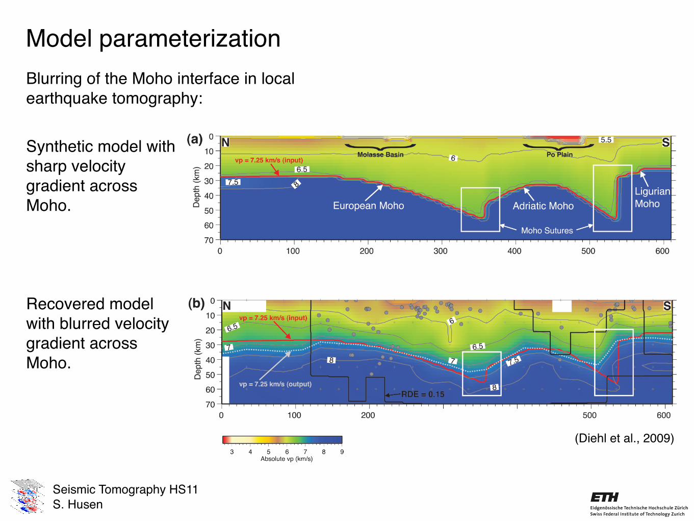
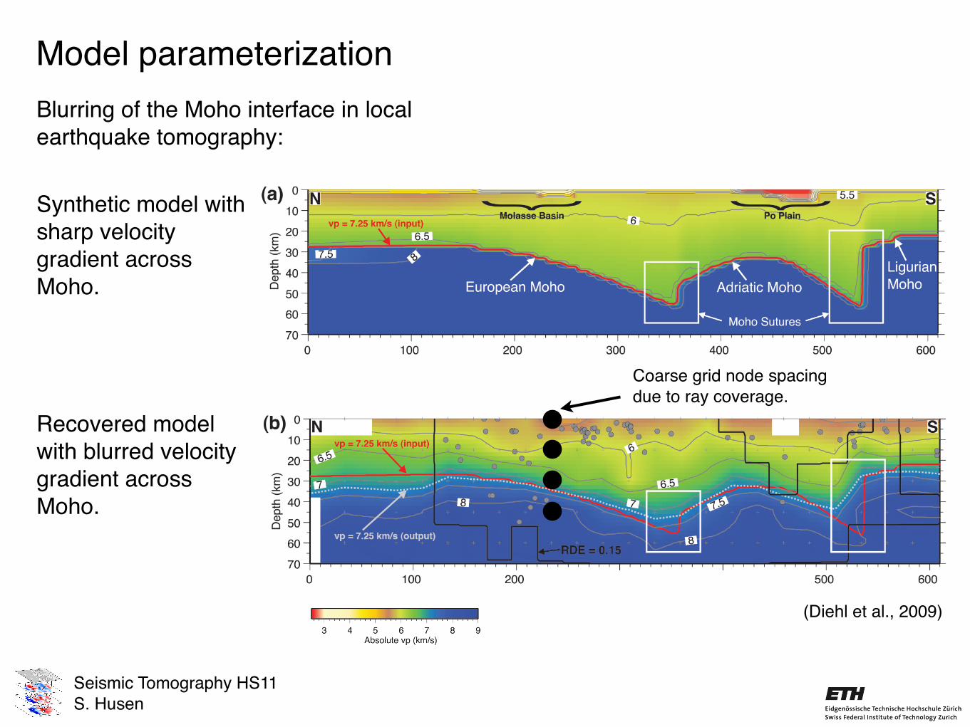
Figure 8. Resolution test and tomographic result as cross-sections along the NFP-20 East/EGT transect (see Fig. 4 for location). (a) Crustal model ofWaldhauser et al. (2002) used to calculate synthetic traveltimes (dense model parametrization). (b) Recovered model after inversion of synthetic traveltimeswith coarse parametrization. Sharp Moho-offsets (regions outlined by white rectangles) are smoothed out in the recovered model. (c) Initial 1-D model usedfor all 3-D inversions. (d) Final inversion result of ‘real’ data set. Fairly and poorly resolved areas are masked. Black lines represent tectonic transect afterSchmid et al. (2004). Position of CSS Mohos after Waldhauser et al. (1998) is indicated by solid yellow line. The suture between European and Adriatic Mohois smoothed out similar to recovered synthetic model, the offset towards Ligurian Moho seems further south in the ‘real’ data. Projected hypocentres (greydots) are located within ±50 km distance off the profile. Focal depths of events labelled as E1 and E2 are discussed in Section 6. Vertical exaggeration for allcross sections is 2:1.
parametrization, initial velocities and inversion parameters as usedfor the ‘real’ data.
The result of the inversion is shown in Fig. 8(b). Well resolvedparts are outlined by the RDE = 0.15 contour line. Compared tothe steep velocity gradient defining the Moho in the input model ofFig. 8(a), the output of the inversion denotes an obviously flatter gra-dient, indicated by the less dense velocity contour lines between 6.5and 8.0 km s!1. This broadening of the velocity gradient is mainlycaused by the coarse parametrization of our model. Furthermore,the initial 1-D model (Fig. 8c) used for the inversion might not bethe optimum choice, since it does not represent the minimum 1-Dmodel of the CSS input model (higher velocities in the upper crustcompared to CSS model).
Although the vP = 6.0 km s!1 contour line indicates some verticalleakage problems (e.g. at 200 and 310 km), it seems not affectedby the Moho topography. From this we conclude that velocitiesbetween 6.5 and 8.0 km s!1 are mainly associated with the Mohogradient in our model parametrization. On the other side, we observea very good agreement between the vP = 7.25 km s!1 contourline of the input model (solid red line in Figs 8a and b) and thevP = 7.25 km s!1 contour line of the inversion result (dashed lightgrey line in Fig. 8b). Therefore, we define the vP = 7.25 km s!1
contour line as the ‘tomography’ Moho in our model. Moho offsets(European/Adriatic and Adriatic/Ligurian) as indicated by kinks
in the CSS model (outlined by white rectangles in Fig. 8a) aresmoothed out in the recovered model (Fig. 8b).
Fig. 8(d) shows the result from the inversion of the ‘real’ dataset as vertical cross-section along the same EGT transect (for lo-cation see Fig. 4). Fairly and poorly resolved areas are masked.Tectonic transect after Schmid et al. (2004) is represented by blacklines and positions of CSS Mohos after Waldhauser et al. (1998)are indicated by solid yellow lines. Solid light grey line denotesthe vP = 7.25 km s!1 contour (tomography Moho) as derived fromthe ‘real’ data set, dashed light grey line corresponds to vP =7.25 km s!1 contour from the inversion of the synthetic data (sameas in Fig. 8b). In general, a rather good agreement is observedbetween tomographic and CSS Moho. Southward dipping of theEuropean Moho, up-doming of the Adriatic Moho and the offsetbetween Adriatic and Ligurian Moho are clearly visible. Further-more, the vP = 7.25 km s!1 contour predicted by the syntheticmodel (dashed light grey line in Figs 8b and d) agrees very wellwith the tomography Moho of the ‘real’ data (solid light grey linein Fig. 8d). Although the ‘real’ data indicates slightly higher veloci-ties in the suture zone between European and Adriatic lower crust, itshows a smoothed offset similar to the recovered synthetic model ofFig. 8(b). Therefore, the existence of a kink or offset in the range ofthe suture zone between European and Adriatic Moho, as present inthe model of Waldhauser et al. (2002) (Fig. 8a), cannot be excluded.
C" 2009 The Authors, GJI, 179, 1133–1147Journal compilation C" 2009 RAS
Blurring of the Moho interface in local earthquake tomography:
Synthetic model with sharp velocity gradient across Moho.
High-resolution 3-D P-wave model of the Alpine crust 1139
Figure 8. Resolution test and tomographic result as cross-sections along the NFP-20 East/EGT transect (see Fig. 4 for location). (a) Crustal model ofWaldhauser et al. (2002) used to calculate synthetic traveltimes (dense model parametrization). (b) Recovered model after inversion of synthetic traveltimeswith coarse parametrization. Sharp Moho-offsets (regions outlined by white rectangles) are smoothed out in the recovered model. (c) Initial 1-D model usedfor all 3-D inversions. (d) Final inversion result of ‘real’ data set. Fairly and poorly resolved areas are masked. Black lines represent tectonic transect afterSchmid et al. (2004). Position of CSS Mohos after Waldhauser et al. (1998) is indicated by solid yellow line. The suture between European and Adriatic Mohois smoothed out similar to recovered synthetic model, the offset towards Ligurian Moho seems further south in the ‘real’ data. Projected hypocentres (greydots) are located within ±50 km distance off the profile. Focal depths of events labelled as E1 and E2 are discussed in Section 6. Vertical exaggeration for allcross sections is 2:1.
parametrization, initial velocities and inversion parameters as usedfor the ‘real’ data.
The result of the inversion is shown in Fig. 8(b). Well resolvedparts are outlined by the RDE = 0.15 contour line. Compared tothe steep velocity gradient defining the Moho in the input model ofFig. 8(a), the output of the inversion denotes an obviously flatter gra-dient, indicated by the less dense velocity contour lines between 6.5and 8.0 km s!1. This broadening of the velocity gradient is mainlycaused by the coarse parametrization of our model. Furthermore,the initial 1-D model (Fig. 8c) used for the inversion might not bethe optimum choice, since it does not represent the minimum 1-Dmodel of the CSS input model (higher velocities in the upper crustcompared to CSS model).
Although the vP = 6.0 km s!1 contour line indicates some verticalleakage problems (e.g. at 200 and 310 km), it seems not affectedby the Moho topography. From this we conclude that velocitiesbetween 6.5 and 8.0 km s!1 are mainly associated with the Mohogradient in our model parametrization. On the other side, we observea very good agreement between the vP = 7.25 km s!1 contourline of the input model (solid red line in Figs 8a and b) and thevP = 7.25 km s!1 contour line of the inversion result (dashed lightgrey line in Fig. 8b). Therefore, we define the vP = 7.25 km s!1
contour line as the ‘tomography’ Moho in our model. Moho offsets(European/Adriatic and Adriatic/Ligurian) as indicated by kinks
in the CSS model (outlined by white rectangles in Fig. 8a) aresmoothed out in the recovered model (Fig. 8b).
Fig. 8(d) shows the result from the inversion of the ‘real’ dataset as vertical cross-section along the same EGT transect (for lo-cation see Fig. 4). Fairly and poorly resolved areas are masked.Tectonic transect after Schmid et al. (2004) is represented by blacklines and positions of CSS Mohos after Waldhauser et al. (1998)are indicated by solid yellow lines. Solid light grey line denotesthe vP = 7.25 km s!1 contour (tomography Moho) as derived fromthe ‘real’ data set, dashed light grey line corresponds to vP =7.25 km s!1 contour from the inversion of the synthetic data (sameas in Fig. 8b). In general, a rather good agreement is observedbetween tomographic and CSS Moho. Southward dipping of theEuropean Moho, up-doming of the Adriatic Moho and the offsetbetween Adriatic and Ligurian Moho are clearly visible. Further-more, the vP = 7.25 km s!1 contour predicted by the syntheticmodel (dashed light grey line in Figs 8b and d) agrees very wellwith the tomography Moho of the ‘real’ data (solid light grey linein Fig. 8d). Although the ‘real’ data indicates slightly higher veloci-ties in the suture zone between European and Adriatic lower crust, itshows a smoothed offset similar to the recovered synthetic model ofFig. 8(b). Therefore, the existence of a kink or offset in the range ofthe suture zone between European and Adriatic Moho, as present inthe model of Waldhauser et al. (2002) (Fig. 8a), cannot be excluded.
C" 2009 The Authors, GJI, 179, 1133–1147Journal compilation C" 2009 RAS
(Diehl et al., 2009)
Seismic Tomography HS11S. Husen
Model parameterization
High-resolution 3-D P-wave model of the Alpine crust 1139
Figure 8. Resolution test and tomographic result as cross-sections along the NFP-20 East/EGT transect (see Fig. 4 for location). (a) Crustal model ofWaldhauser et al. (2002) used to calculate synthetic traveltimes (dense model parametrization). (b) Recovered model after inversion of synthetic traveltimeswith coarse parametrization. Sharp Moho-offsets (regions outlined by white rectangles) are smoothed out in the recovered model. (c) Initial 1-D model usedfor all 3-D inversions. (d) Final inversion result of ‘real’ data set. Fairly and poorly resolved areas are masked. Black lines represent tectonic transect afterSchmid et al. (2004). Position of CSS Mohos after Waldhauser et al. (1998) is indicated by solid yellow line. The suture between European and Adriatic Mohois smoothed out similar to recovered synthetic model, the offset towards Ligurian Moho seems further south in the ‘real’ data. Projected hypocentres (greydots) are located within ±50 km distance off the profile. Focal depths of events labelled as E1 and E2 are discussed in Section 6. Vertical exaggeration for allcross sections is 2:1.
parametrization, initial velocities and inversion parameters as usedfor the ‘real’ data.
The result of the inversion is shown in Fig. 8(b). Well resolvedparts are outlined by the RDE = 0.15 contour line. Compared tothe steep velocity gradient defining the Moho in the input model ofFig. 8(a), the output of the inversion denotes an obviously flatter gra-dient, indicated by the less dense velocity contour lines between 6.5and 8.0 km s!1. This broadening of the velocity gradient is mainlycaused by the coarse parametrization of our model. Furthermore,the initial 1-D model (Fig. 8c) used for the inversion might not bethe optimum choice, since it does not represent the minimum 1-Dmodel of the CSS input model (higher velocities in the upper crustcompared to CSS model).
Although the vP = 6.0 km s!1 contour line indicates some verticalleakage problems (e.g. at 200 and 310 km), it seems not affectedby the Moho topography. From this we conclude that velocitiesbetween 6.5 and 8.0 km s!1 are mainly associated with the Mohogradient in our model parametrization. On the other side, we observea very good agreement between the vP = 7.25 km s!1 contourline of the input model (solid red line in Figs 8a and b) and thevP = 7.25 km s!1 contour line of the inversion result (dashed lightgrey line in Fig. 8b). Therefore, we define the vP = 7.25 km s!1
contour line as the ‘tomography’ Moho in our model. Moho offsets(European/Adriatic and Adriatic/Ligurian) as indicated by kinks
in the CSS model (outlined by white rectangles in Fig. 8a) aresmoothed out in the recovered model (Fig. 8b).
Fig. 8(d) shows the result from the inversion of the ‘real’ dataset as vertical cross-section along the same EGT transect (for lo-cation see Fig. 4). Fairly and poorly resolved areas are masked.Tectonic transect after Schmid et al. (2004) is represented by blacklines and positions of CSS Mohos after Waldhauser et al. (1998)are indicated by solid yellow lines. Solid light grey line denotesthe vP = 7.25 km s!1 contour (tomography Moho) as derived fromthe ‘real’ data set, dashed light grey line corresponds to vP =7.25 km s!1 contour from the inversion of the synthetic data (sameas in Fig. 8b). In general, a rather good agreement is observedbetween tomographic and CSS Moho. Southward dipping of theEuropean Moho, up-doming of the Adriatic Moho and the offsetbetween Adriatic and Ligurian Moho are clearly visible. Further-more, the vP = 7.25 km s!1 contour predicted by the syntheticmodel (dashed light grey line in Figs 8b and d) agrees very wellwith the tomography Moho of the ‘real’ data (solid light grey linein Fig. 8d). Although the ‘real’ data indicates slightly higher veloci-ties in the suture zone between European and Adriatic lower crust, itshows a smoothed offset similar to the recovered synthetic model ofFig. 8(b). Therefore, the existence of a kink or offset in the range ofthe suture zone between European and Adriatic Moho, as present inthe model of Waldhauser et al. (2002) (Fig. 8a), cannot be excluded.
C" 2009 The Authors, GJI, 179, 1133–1147Journal compilation C" 2009 RAS
Blurring of the Moho interface in local earthquake tomography:
High-resolution 3-D P-wave model of the Alpine crust 1139
Figure 8. Resolution test and tomographic result as cross-sections along the NFP-20 East/EGT transect (see Fig. 4 for location). (a) Crustal model ofWaldhauser et al. (2002) used to calculate synthetic traveltimes (dense model parametrization). (b) Recovered model after inversion of synthetic traveltimeswith coarse parametrization. Sharp Moho-offsets (regions outlined by white rectangles) are smoothed out in the recovered model. (c) Initial 1-D model usedfor all 3-D inversions. (d) Final inversion result of ‘real’ data set. Fairly and poorly resolved areas are masked. Black lines represent tectonic transect afterSchmid et al. (2004). Position of CSS Mohos after Waldhauser et al. (1998) is indicated by solid yellow line. The suture between European and Adriatic Mohois smoothed out similar to recovered synthetic model, the offset towards Ligurian Moho seems further south in the ‘real’ data. Projected hypocentres (greydots) are located within ±50 km distance off the profile. Focal depths of events labelled as E1 and E2 are discussed in Section 6. Vertical exaggeration for allcross sections is 2:1.
parametrization, initial velocities and inversion parameters as usedfor the ‘real’ data.
The result of the inversion is shown in Fig. 8(b). Well resolvedparts are outlined by the RDE = 0.15 contour line. Compared tothe steep velocity gradient defining the Moho in the input model ofFig. 8(a), the output of the inversion denotes an obviously flatter gra-dient, indicated by the less dense velocity contour lines between 6.5and 8.0 km s!1. This broadening of the velocity gradient is mainlycaused by the coarse parametrization of our model. Furthermore,the initial 1-D model (Fig. 8c) used for the inversion might not bethe optimum choice, since it does not represent the minimum 1-Dmodel of the CSS input model (higher velocities in the upper crustcompared to CSS model).
Although the vP = 6.0 km s!1 contour line indicates some verticalleakage problems (e.g. at 200 and 310 km), it seems not affectedby the Moho topography. From this we conclude that velocitiesbetween 6.5 and 8.0 km s!1 are mainly associated with the Mohogradient in our model parametrization. On the other side, we observea very good agreement between the vP = 7.25 km s!1 contourline of the input model (solid red line in Figs 8a and b) and thevP = 7.25 km s!1 contour line of the inversion result (dashed lightgrey line in Fig. 8b). Therefore, we define the vP = 7.25 km s!1
contour line as the ‘tomography’ Moho in our model. Moho offsets(European/Adriatic and Adriatic/Ligurian) as indicated by kinks
in the CSS model (outlined by white rectangles in Fig. 8a) aresmoothed out in the recovered model (Fig. 8b).
Fig. 8(d) shows the result from the inversion of the ‘real’ dataset as vertical cross-section along the same EGT transect (for lo-cation see Fig. 4). Fairly and poorly resolved areas are masked.Tectonic transect after Schmid et al. (2004) is represented by blacklines and positions of CSS Mohos after Waldhauser et al. (1998)are indicated by solid yellow lines. Solid light grey line denotesthe vP = 7.25 km s!1 contour (tomography Moho) as derived fromthe ‘real’ data set, dashed light grey line corresponds to vP =7.25 km s!1 contour from the inversion of the synthetic data (sameas in Fig. 8b). In general, a rather good agreement is observedbetween tomographic and CSS Moho. Southward dipping of theEuropean Moho, up-doming of the Adriatic Moho and the offsetbetween Adriatic and Ligurian Moho are clearly visible. Further-more, the vP = 7.25 km s!1 contour predicted by the syntheticmodel (dashed light grey line in Figs 8b and d) agrees very wellwith the tomography Moho of the ‘real’ data (solid light grey linein Fig. 8d). Although the ‘real’ data indicates slightly higher veloci-ties in the suture zone between European and Adriatic lower crust, itshows a smoothed offset similar to the recovered synthetic model ofFig. 8(b). Therefore, the existence of a kink or offset in the range ofthe suture zone between European and Adriatic Moho, as present inthe model of Waldhauser et al. (2002) (Fig. 8a), cannot be excluded.
C" 2009 The Authors, GJI, 179, 1133–1147Journal compilation C" 2009 RAS
Synthetic model with sharp velocity gradient across Moho.
Recovered model with blurred velocity gradient across Moho.
High-resolution 3-D P-wave model of the Alpine crust 1139
Figure 8. Resolution test and tomographic result as cross-sections along the NFP-20 East/EGT transect (see Fig. 4 for location). (a) Crustal model ofWaldhauser et al. (2002) used to calculate synthetic traveltimes (dense model parametrization). (b) Recovered model after inversion of synthetic traveltimeswith coarse parametrization. Sharp Moho-offsets (regions outlined by white rectangles) are smoothed out in the recovered model. (c) Initial 1-D model usedfor all 3-D inversions. (d) Final inversion result of ‘real’ data set. Fairly and poorly resolved areas are masked. Black lines represent tectonic transect afterSchmid et al. (2004). Position of CSS Mohos after Waldhauser et al. (1998) is indicated by solid yellow line. The suture between European and Adriatic Mohois smoothed out similar to recovered synthetic model, the offset towards Ligurian Moho seems further south in the ‘real’ data. Projected hypocentres (greydots) are located within ±50 km distance off the profile. Focal depths of events labelled as E1 and E2 are discussed in Section 6. Vertical exaggeration for allcross sections is 2:1.
parametrization, initial velocities and inversion parameters as usedfor the ‘real’ data.
The result of the inversion is shown in Fig. 8(b). Well resolvedparts are outlined by the RDE = 0.15 contour line. Compared tothe steep velocity gradient defining the Moho in the input model ofFig. 8(a), the output of the inversion denotes an obviously flatter gra-dient, indicated by the less dense velocity contour lines between 6.5and 8.0 km s!1. This broadening of the velocity gradient is mainlycaused by the coarse parametrization of our model. Furthermore,the initial 1-D model (Fig. 8c) used for the inversion might not bethe optimum choice, since it does not represent the minimum 1-Dmodel of the CSS input model (higher velocities in the upper crustcompared to CSS model).
Although the vP = 6.0 km s!1 contour line indicates some verticalleakage problems (e.g. at 200 and 310 km), it seems not affectedby the Moho topography. From this we conclude that velocitiesbetween 6.5 and 8.0 km s!1 are mainly associated with the Mohogradient in our model parametrization. On the other side, we observea very good agreement between the vP = 7.25 km s!1 contourline of the input model (solid red line in Figs 8a and b) and thevP = 7.25 km s!1 contour line of the inversion result (dashed lightgrey line in Fig. 8b). Therefore, we define the vP = 7.25 km s!1
contour line as the ‘tomography’ Moho in our model. Moho offsets(European/Adriatic and Adriatic/Ligurian) as indicated by kinks
in the CSS model (outlined by white rectangles in Fig. 8a) aresmoothed out in the recovered model (Fig. 8b).
Fig. 8(d) shows the result from the inversion of the ‘real’ dataset as vertical cross-section along the same EGT transect (for lo-cation see Fig. 4). Fairly and poorly resolved areas are masked.Tectonic transect after Schmid et al. (2004) is represented by blacklines and positions of CSS Mohos after Waldhauser et al. (1998)are indicated by solid yellow lines. Solid light grey line denotesthe vP = 7.25 km s!1 contour (tomography Moho) as derived fromthe ‘real’ data set, dashed light grey line corresponds to vP =7.25 km s!1 contour from the inversion of the synthetic data (sameas in Fig. 8b). In general, a rather good agreement is observedbetween tomographic and CSS Moho. Southward dipping of theEuropean Moho, up-doming of the Adriatic Moho and the offsetbetween Adriatic and Ligurian Moho are clearly visible. Further-more, the vP = 7.25 km s!1 contour predicted by the syntheticmodel (dashed light grey line in Figs 8b and d) agrees very wellwith the tomography Moho of the ‘real’ data (solid light grey linein Fig. 8d). Although the ‘real’ data indicates slightly higher veloci-ties in the suture zone between European and Adriatic lower crust, itshows a smoothed offset similar to the recovered synthetic model ofFig. 8(b). Therefore, the existence of a kink or offset in the range ofthe suture zone between European and Adriatic Moho, as present inthe model of Waldhauser et al. (2002) (Fig. 8a), cannot be excluded.
C" 2009 The Authors, GJI, 179, 1133–1147Journal compilation C" 2009 RAS
Coarse grid node spacing due to ray coverage.
(Diehl et al., 2009)

Seismic Tomography HS11S. Husen
Model parameterization
• There is no perfect solution to the problem of model parameterization.
• Model parameterization has an effect on the solution and solution quality.
• A chosen model parameterization need to be tested by means of synthetic velocity models.