Seismic Risk of Structures and the Economic Issues of

Chapter 1

© 2012 Kalantari, licensee InTech. This is an open access chapter distributed under the terms of the Creative Commons Attribution License (http://creativecommons.org/licenses/by/3.0), which permits unrestricted use, distribution, and reproduction in any medium, provided the original work is properly cited.

Seismic Risk of Structures and the Economic Issues of Earthquakes

Afshin Kalantari

Additional information is available at the end of the chapter

http://dx.doi.org/10.5772/50789

1. Introduction

As one of the most devastating natural events, earthquakes impose economic challenges on communities and governments. The number of human and economic assets at risk is growing as megacities and urban areas develop all over the world. This increasing risk has been plotted in the damage and loss reports after the great earthquakes.

The 1975 Tangshan (China) earthquake killed about 200,000 people. The 1994 Northridge, (USA) earthquake left 57 dead and about 8,700 injured. The country experienced around $42 billion in losses due to it. The 1995 earthquake in Kobe (Japan) caused about 6,000 fatalities and over $120 Billion in economic loss. The August 1996 Izmit (Turkey) earthquake killed 20,000 people and caused $12 billion in economic loss. The 1999 Chi-chi (Taiwan) earthquake caused an estimated $8 billion in loss. The 2006 Gujarat (India) earthquake saw around 18,000 fatalities and 330,000 demolished buildings [1]. The Sichuan (China) earthquake, on May 12th 2008 left 88,000 people dead or missing and nearly 400,000 injured. That earthquake damaged or destroyed millions of homes, leaving five million homeless. It also caused extensive damage to basic infrastructure, including schools, hospitals, roads and water systems. The event cost around $29 billion in direct loss alone [2]. The devastating earthquake of March 2011 with its resulting tsunami along the east coast of Japan is known to be the world's most costly earthquake. The World Bank estimated the cost at $235 billion while government estimates reported the number at $305 billion. The event left 8,700 dead and more than 13,000 missing [3].

As has been shown, earthquake events have not only inflicted human and physical damage, they have also been able to cause considerable economic conflict in vulnerable cities and regions. The importance of the economic issues and the consequences of earthquakes attracted the attention of engineers and provided new research and working opportunities

Earthquake Engineering 4

for engineers, who up until then had been concerned only with risk reduction options through engineering strategies [4].

Seismic loss estimation is an expertise provided by earthquake engineering and the manner in which it can be employed in the processes of assessing seismic loss and managing the financial and economical risk associated with earthquakes through more beneficial retrofit methods will be discussed. The methodology provides a useful tool for comparing different engineering alternatives from a seismic-risk-point of view based on a Performance Based Earthquake Engineering (PBEE) framework [5]. Next, an outline of the regional economic models employed for the assessment of earthquakes’ impact on economies will be briefly introduced.

1.1. The economic consequences of earthquakes

The economic consequences of earthquakes may occur both before and after the seismic event itself [6]. However, the focus of this chapter will be on those which occur after earthquakes. The consequences and effects of earthquakes may be classified in terms of their primary or direct effects and their secondary or indirect effects. The indirect effects are sometimes referred to by economists as higher-order effects. The primary (direct) effects of an earthquake appear immediately after it as social and physical damage. The secondary (indirect) effects take into account the system-wide impact of flow losses through inter-industry relationships and economic sectors. For example, where damage occurs to a bridge then its inability to serve to passing vehicles is considered a primary or direct loss, while if the flow of the row material to a manufacturing plant in another area is interrupted due to the inability of passing traffic to cross the bridge, the loss due to the business’s interruption in this plant is called secondary or indirect loss. A higher-order effect is another term as an alternative to indirect or secondary effects which has been proposed by economists [7]. These potential effects of earthquakes may be categorized as: "social or human", "physical" and "economic" effects. This is summarized in Table 1 [8].

The term ‘total impact’ accordingly refers to the summation of direct (first-order effects) and indirect losses (higher-order effects). Various economic frameworks have been introduced to assess the higher-order effects of an earthquake.

With a three-sector hypothesis of an economy, it may be demonstrated in terms of a breakdown as three sectors: the primary sector as raw materials, the secondary sector as manufacturing and the tertiary sector as services. The interaction of these sectors after suffering seismic loss and the relative effects on each other requires study through proper economic models.

2. The estimation of seismic loss of structures in the PBEE framework

The PBEE process can be expressed in terms of a four-step analysis, including [9-10]:

Hazard analysis, which results in Intensity Measures (IMs) for the facility under study,

Seismic Risk of Structures and Earthquake Economic Issues 5

Structural analysis, which gives the Engineering Demand Parameters (EDPs) required for damage analysis,

Damage analysis, which compares the EDPs with the Damage Measure in order to decide for the failure of the facility, and;

Loss Analysis, which evaluates the occurrence of Decision Variables (DVs) due to failures.

Social or human

effects Physical effects Economic effects

Primary effects (Direct or first-order)

Fatalities Injuries Loss of income or employment opportunities Homelessness

Ground deformation and loss of ground quality Collapse and structural damage to buildings and infrastructure Non-structural damage to buildings and infrastructure (e.g., component damage)

Disruption of business due to damage to industrial plants and equipment Loss of productive work force, through fatalities, injuries and relief efforts Disruption of communications networks Cost of response and relief

Secondary effects (indirect or higher-order)

Disease or permanent disability Psychological impact of injury, Bereavement, shock Loss of social cohesion due to disruption of community Political unrest when government response is perceived as inadequate

Reduction of the seismic capacity of damaged structure which are not repaired Progressive deterioration of damaged buildings and infrastructure which are not repaired

Losses borne by the insurance industry, weakening the insurance market and increasing the premiums Losses of markets and trade opportunities,

Table 1. Effects from Earthquakes [8]

Considering the results of each step as a conditional event following the previous step and all of the parameters as independent random parameters, the process can be expressed in terms of a triple integral, as shown below, which is an application of the total probability theorem [11]:


( ) = ∭ [ | ]| [ | ]| [ | | [ ] (1)

The performance of a structural system or lifeline is described by comparing demand and capacity parameters. In earthquake engineering, the excitation, demand and capacity parameters are random variables. Therefore, probabilistic techniques are required in order to estimate the response of the system and provide information about the availability or failure of the facility after loading. The concept is included in the reliability design approach, which is usually employed for this purpose.

2.1. Probabilistic seismic demand analysis through a reliability-based design approach

The reliability of a structural system or lifeline may be referred to as the ability of the system or its components to perform their required functions under stated conditions for a specified period of time. Because of uncertainties in loading and capacity, the subject usually includes probabilistic methods and is often made through indices such as a safety index or the probability of the failure of the structure or lifeline.

2.1.1. Reliability index and failure

To evaluate the seismic performance of the structures, performance functions are defined. Let us assume that z=g(x1, x2, …,xn) is taken as a performance function. As such, failure or damage occurs when z<0. The probability of failure, pf, is expressed as follows:

Pf=P[z<0] (2)

Simply assume that z=EDP-C where EDP stands for Engineering Demand Parameter and C is the seismic capacity of the structure.

Damage or failure in a structural system or lifeline occurs when the Engineering Demand Parameter exceeds the capacity provided. For example, in a bridge structural damage may refer to the unseating of the deck, the development of a plastic hinge at the bottom of piers or damage due to the pounding of the decks to the abutments, etc.

Given that EDP and C are random parameters having the expected or mean values of µEDP and µC and standard deviation of σEDP and σC, the “safety index” or “reliability index”, β, is defined as:

= (3)

It has been observed that the random variables such as "EDP" or "C" follow normal or log-normal distribution. Accordingly, the performance function, z, also will follow the same distribution. Accordingly, probability of failure (or damage occurrence) may be expressed as a function of safety index, as follows:


Pf=φ (- β)=1- φ (β) (4)

where φ( ) is a log-normal distribution function.

2.1.2. Engineering demand parameters

The Engineering Demand Parameters describe the response of the structural framing and the non-structural components and contents resulting from earthquake shaking. The parameters are calculated by structural response simulations using the IMs and corresponding earthquake motions. The ground motions should capture the important characteristics of earthquake ground motion which affect the response of the structural framing and non-structural components and building contents. During the loss and risk estimation studies, the EDP with a greater correlation with damage and loss variables must be employed.

The EDPs were categorized in the ATC 58 task report as either direct or processed [9]. Direct EDPs are those calculated directly by analysis or simulation and contribute to the risk assessment through the calculation of P[EDP | IM]; examples of direct EDPs include interstory drift and beam plastic rotation. Processed EDPs - for example, a damage index - are derived from the values of direct EDPs and data on component or system capacities. Processed EDPs could be considered as either EDPs or as Damage Measures (DMs) and, as such, could contribute to risk assessment through P[DM | EDP]. Direct EDPs are usually introduced in codes and design regulations. For example, the 2000 NEHRP Recommended Provisions for Seismic Regulations for Buildings and Other Structures introduces the EDPs presented in Table 2 for the seismic design of reinforced concrete moment frames [12-13]:

Reinforced concrete moment framesAxial force, bending moment and shear force in columns

Bending moment and shear force in beams Shear force in beam-column joints

Shear force and bending moments in slabs Bearing and lateral pressures beneath foundations

Interstory drift (and interstory drift angle)

Table 2. EDPs required for the seismic design of reinforced concrete moment frames by [12-13]

Processed EDPs are efficient parameters which could serve as a damage index during loss and risk estimation for structural systems and facilities. A Damage Index (DI), as a single-valued damage characteristic, can be considered to be a processed EDP [10]. Traditionally, DIs have been used to express performance in terms of a value between 0 (no damage) and 1 (collapse or an ultimate state). An extension of this approach is the damage spectrum, which takes on values between 0 (no damage) and 1 (collapse) as a function of a period. A detailed summary of the available DIs is available in [14].

Park and Angin [15] developed one of the most widely-known damage indices. The index is a linear combination of structural displacement and hysteretic energy, as shown in the equation:


= + (5)

where umax and uc are maximum and capacity displacement of the structure, respectively, Eh is the hysteresis energy, Fy is the yielding force and β is a constant.

See Powell and Allahabadi, Fajfar, Mehanny and Deierlein, as well as Bozorgnia and Bertero for more information about other DIs in [16-19].

2.2. Seismic fragility

The seismic fragility of a structure refers to the probability that the Engineering Demand Parameter (EDP) will exceed seismic capacity (C) upon the condition of the occurrence of a specific Intensity Measure (IM). In other words, seismic fragility is probability of failure, Pf, on the condition of the occurrence of a specific intensity measure, as shown below:

Fragility=P [EDP>C|IM] (6)

In a fragility curve, the horizontal axis introduces the IM and the vertical axis corresponds to the probability of failure, Pf. This curve demonstrates how the variation of intensity measure affects the probability of failure of the structure.

Statistical approach, analytical and numerical simulations, and the use of expert opinion provide methods for developing fragility curves.

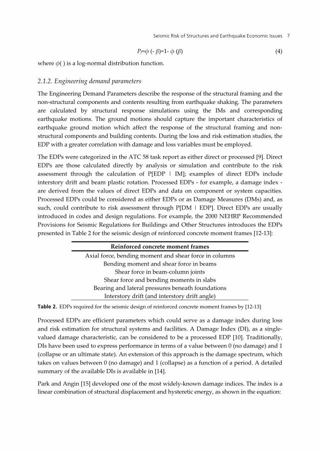
2.2.1. Statistical approach

With a statistical approach, a sufficient amount of real damage-intensity data after earthquakes is employed to generate the seismic fragility data. As an example, Figure 1 demonstrates the empirical fragility curves for a concrete moment resisting frame, according to the data collected after Northridge earthquake [20].

Figure 1. Empirical fragility curves for a concrete moment resisting frame building class according to the data collected after the Northridge Earthquake, [20].


2.2.2. Analytical approach

With an analytical approach, a numerical model of the structure is usually analysed by nonlinear dynamic analysis methods in order to calculate the EDPs and compare the results with the capacity to decide about the failure of the structure. The works in [21-24] are examples of analytical fragility curves for highway bridge structures by Hwang et al. 2001, Choi et al. 2004, Padgett et al., 2008, and Padgett et al 2008 .

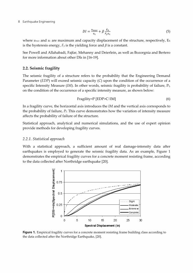
Figure 2 demonstrates the steps for computing seismic fragility in analytical approach.

Figure 2. Procedure for generating analytical fragility curves

To overcome the uncertainties in input excitation or the developed model, usually adequate number of records and several numerical models are required so that the dispersion of the calculated data will be limited and acceptable. This is usually elaborating and increases the cost of the generation of fragility data in this approach. Probabilistic demand models are usually one of the outputs of nonlinear dynamic analysis. Probabilistic demand models establish a relationship between the intensity measure and the engineering demand parameter. Bazorro and Cornell proposed the model given below [25]:

EDP = ( ) (7)

where EDP is the average value of EDP and a and b are constants. The model has the capability to be presented as linear in a logarithmic space such that:

ln(EDP) = ln( ) + bln( ) (8)

Assuming a log-normal distribution for fragility values, they are then estimated using the following equation:

[ > | ] = ∅ ( )̅| (9)


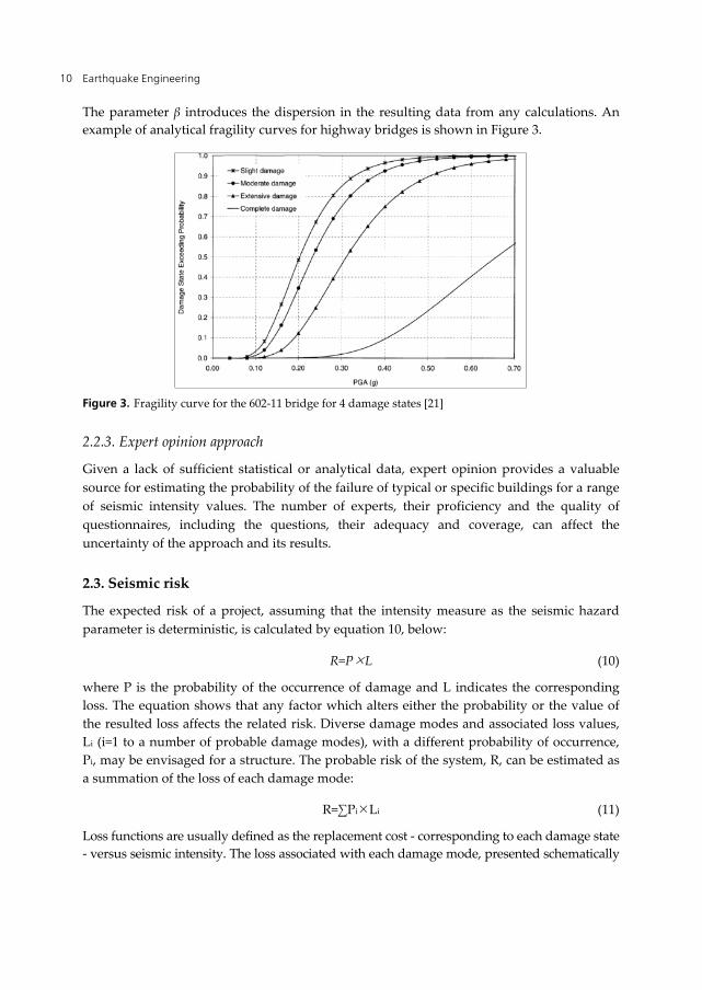
The parameter β introduces the dispersion in the resulting data from any calculations. An example of analytical fragility curves for highway bridges is shown in Figure 3.

Figure 3. Fragility curve for the 602-11 bridge for 4 damage states [21]

2.2.3. Expert opinion approach

Given a lack of sufficient statistical or analytical data, expert opinion provides a valuable source for estimating the probability of the failure of typical or specific buildings for a range of seismic intensity values. The number of experts, their proficiency and the quality of questionnaires, including the questions, their adequacy and coverage, can affect the uncertainty of the approach and its results.

2.3. Seismic risk

The expected risk of a project, assuming that the intensity measure as the seismic hazard parameter is deterministic, is calculated by equation 10, below:

R=PL (10)

where P is the probability of the occurrence of damage and L indicates the corresponding loss. The equation shows that any factor which alters either the probability or the value of the resulted loss affects the related risk. Diverse damage modes and associated loss values, Li (i=1 to a number of probable damage modes), with a different probability of occurrence, Pi, may be envisaged for a structure. The probable risk of the system, R, can be estimated as a summation of the loss of each damage mode:

R=∑PiLi (11)

Loss functions are usually defined as the replacement cost - corresponding to each damage state - versus seismic intensity. The loss associated with each damage mode, presented schematically


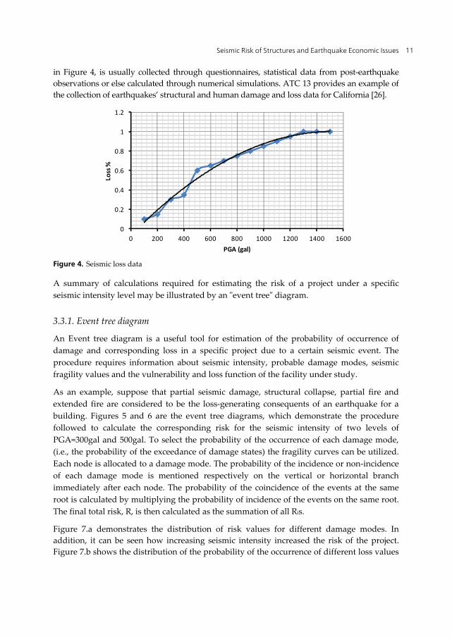
in Figure 4, is usually collected through questionnaires, statistical data from post-earthquake observations or else calculated through numerical simulations. ATC 13 provides an example of the collection of earthquakes’ structural and human damage and loss data for California [26].

Figure 4. Seismic loss data

A summary of calculations required for estimating the risk of a project under a specific seismic intensity level may be illustrated by an "event tree" diagram.

3.3.1. Event tree diagram

An Event tree diagram is a useful tool for estimation of the probability of occurrence of damage and corresponding loss in a specific project due to a certain seismic event. The procedure requires information about seismic intensity, probable damage modes, seismic fragility values and the vulnerability and loss function of the facility under study.

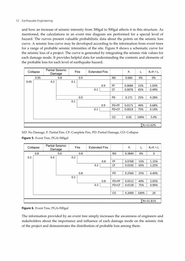
As an example, suppose that partial seismic damage, structural collapse, partial fire and extended fire are considered to be the loss-generating consequents of an earthquake for a building. Figures 5 and 6 are the event tree diagrams, which demonstrate the procedure followed to calculate the corresponding risk for the seismic intensity of two levels of PGA=300gal and 500gal. To select the probability of the occurrence of each damage mode, (i.e., the probability of the exceedance of damage states) the fragility curves can be utilized. Each node is allocated to a damage mode. The probability of the incidence or non-incidence of each damage mode is mentioned respectively on the vertical or horizontal branch immediately after each node. The probability of the coincidence of the events at the same root is calculated by multiplying the probability of incidence of the events on the same root. The final total risk, R, is then calculated as the summation of all Ris.

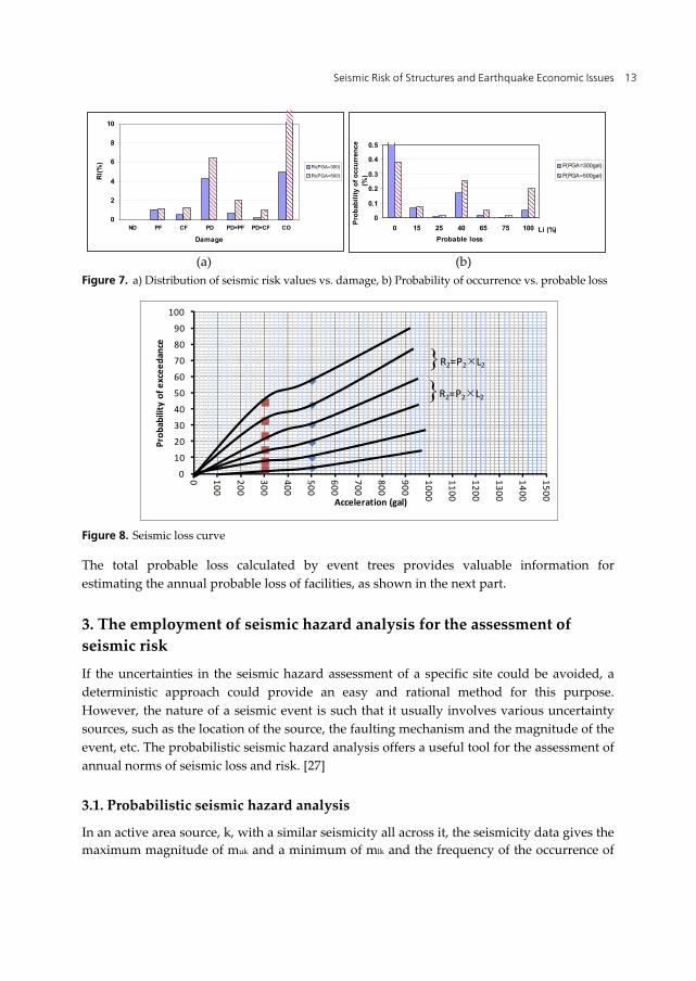
Figure 7.a demonstrates the distribution of risk values for different damage modes. In addition, it can be seen how increasing seismic intensity increased the risk of the project. Figure 7.b shows the distribution of the probability of the occurrence of different loss values

0

0.2

0.4

0.6

0.8

1

1.2

0 200 400 600 800 1000 1200 1400 1600

Loss

%

PGA (gal)


and how an increase of seismic intensity from 300gal to 500gal affects it in this structure. As mentioned, the calculations in an event tree diagram are performed for a special level of hazard. The curves present valuable probabilistic data about the points on the seismic loss curve. A seismic loss curve may be developed according to the information from event trees for a range of probable seismic intensities of the site. Figure 8 shows a schematic curve for the seismic loss of a project. The curve is generated by integrating the seismic risk values for each damage mode. It provides helpful data for understanding the contents and elements of the probable loss for each level of earthquake hazard.

ND: No Damage, F: Partial Fire, CF: Complete Fire, PD: Partial Damage, CO: Collapse

Figure 5. Event Tree, PGA=300gal

Figure 6. Event Tree, PGA=500gal

The information provided by an event tree simply increases the awareness of engineers and stakeholders about the importance and influence of each damage mode on the seismic risk of the project and demonstrates the distribution of probable loss among them.

Ri=PiLi Li Pi Extended Fire Fire Partial Seismic

Damage Collapse

0% 0% 0.684 ND 0.9 0.8 0.95 0.1 0.2 0.05

1.03% 15% 0.0684 PF 0.9 0.49% 65% 0.0076 CF 0.1

4.28% 25% 0.171 PD 0.9

0.1 0.68% 40% 0.0171 PD+PF 0.9 0.14% 75% 0.0019 PD+CF 0.1

5.0% 100% 0.05 CO

∑Ri=11.62%

Ri=PiLi Li Pi Extended Fire Fire Partial Seismic

Damage Collapse

0 0% 0.3840 ND 0.8 0.6 0.8 0.2 0.4 0.2

1.15% 15% 0.0768 PF 0.8 1.25% 65% 0.0192 CF 0.2

6.40% 25% 0.2560 PD 0.8

0.2 2.05% 40% 0.0512 PD+PF 0.8 0.96% 75% 0.0128 PD+CF 0.2

20 100% 0.2000 CO

∑Ri=31.81%


Figure 7. a) Distribution of seismic risk values vs. damage, b) Probability of occurrence vs. probable loss

Figure 8. Seismic loss curve

The total probable loss calculated by event trees provides valuable information for estimating the annual probable loss of facilities, as shown in the next part.

3. The employment of seismic hazard analysis for the assessment of seismic risk

If the uncertainties in the seismic hazard assessment of a specific site could be avoided, a deterministic approach could provide an easy and rational method for this purpose. However, the nature of a seismic event is such that it usually involves various uncertainty sources, such as the location of the source, the faulting mechanism and the magnitude of the event, etc. The probabilistic seismic hazard analysis offers a useful tool for the assessment of annual norms of seismic loss and risk. [27]

3.1. Probabilistic seismic hazard analysis

In an active area source, k, with a similar seismicity all across it, the seismicity data gives the maximum magnitude of muk and a minimum of mlk and the frequency of the occurrence of

0

10

20

30

40

50

60

70

80

90

100

0 100

200

300

400

500

600

700

800

900

1000

1100

1200

1300

1400

1500Pr

obab

ility

of e

xcee

danc

e

Acceleration (gal)

}R2=P2L2

}R2=P2L2

0

2

4

6

8

10

ND PF CF PD PD+PF PD+CF CO

Damage

Ri(%

)

Ri(PGA=300)

Ri(PGA=500)

Probable loss

0

0.1

0.2

0.3

0.4

0.5

0 15 25 40 65 75 100 Li (%)

Prob

abili

ty o

f occ

urre

nce

(%)

P(PGA=300gal)

P(PGA=500gal)

(a) (b)


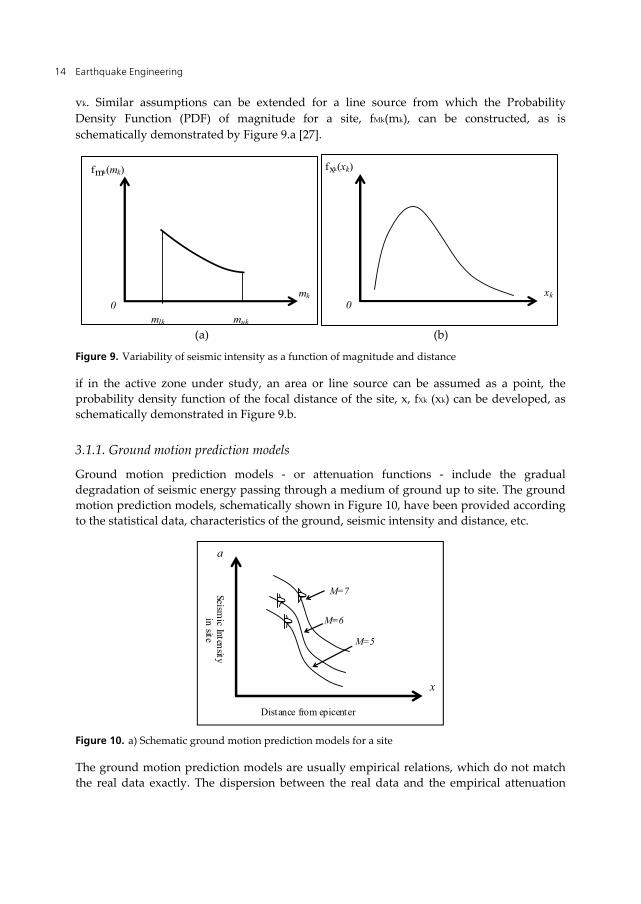
vk. Similar assumptions can be extended for a line source from which the Probability Density Function (PDF) of magnitude for a site, fMk(mk), can be constructed, as is schematically demonstrated by Figure 9.a [27].

Figure 9. Variability of seismic intensity as a function of magnitude and distance

if in the active zone under study, an area or line source can be assumed as a point, the probability density function of the focal distance of the site, x, fXk (xk) can be developed, as schematically demonstrated in Figure 9.b.

3.1.1. Ground motion prediction models

Ground motion prediction models - or attenuation functions - include the gradual degradation of seismic energy passing through a medium of ground up to site. The ground motion prediction models, schematically shown in Figure 10, have been provided according to the statistical data, characteristics of the ground, seismic intensity and distance, etc.

Figure 10. a) Schematic ground motion prediction models for a site

The ground motion prediction models are usually empirical relations, which do not match the real data exactly. The dispersion between the real data and the empirical attenuation

a

x

Seismic Intensity

in site

Distance from epicenter

M=7

M=6

M=5

fmk(mk)

mk0

mlk muk

fxk(xk)

xk 0

(a) (b)


relations may be modelled by a probability density function f(am, x) which shows the distribution density function of intensity a if a seismic event with a magnitude of m occurs at a distance x from the site. Figure 11 shows how f(am, x) changes when an intensity measure a varies.

Figure 11. Probability of exceedance from a specific intensity using a probability density function

According to the above-mentioned collected data, the annual rate of earthquakes with an intensity (acceleration) larger than a, v(a) can be calculated from the following equation:

, d duk

k klkk

mk A k k M k X k k ka m

k x

P a m x f m f x m x (12)

Where, PA(amk, xu) stands for the probability of occurrence of an earthquake with an intensity larger than a at a site with an attenuation relation of fA(am,x).

Poison process is usually employed to model the rate of the occurrence of earthquakes within specific duration. For an earthquake with an annual probability of occurrence of (a), the probability of the occurrence of n earthquakes of intensity greater than a within t years is given by:

exp

( , , )!

nv a t v a t

P n t an

(13)

Meanwhile, the annual probability of exceedance from the intensity a, P(a) can be expressed as:

1 0,1, 1 expP a P a v a (14)

The time interval of earthquakes with an intensity exceeding a is called the return period and is shown as Ta. The parameter can be calculated first knowing that the probability of T is longer than t:

fA(a|m,x)

a

PDF for variations of

attenuation function

Intensity (PGA, …)

PA(a|m,x)


P P 0, , expT t t a v a t (15)

then the probability distribution function of Ta becomes:

TF 1 P 1 expat T t v a t (16)

Accordingly, the probability density function of T, fT, is derived by taking a derivation of the above FT function:

expTf t v a v a t (17)

The return period is known as the mean value of T and can be calculated as:

1 /a

a TT E t tf t dt v a (18)

The probability density function, fA(a), the accumulative probability, FA(a), and the annual probability of exceedance function, P(a), for intensity a (for example PGA), are related to each other, as shown below:

aA AF a f a da

(19)

AaP a f a da

(20)

1 AP a F a (21)

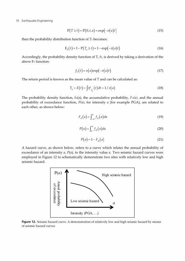
A hazard curve, as shown below, refers to a curve which relates the annual probability of exceedance of an intensity a, P(a), to the intensity value a. Two seismic hazard curves were employed in Figure 12 to schematically demonstrate two sites with relatively low and high seismic hazard.

Figure 12. Seismic hazard curve. A demonstration of relatively low and high seismic hazard by means of seismic hazard curves

P(a)

a

Annul probability

of exceedance

Intensity (PGA, …)

Low seismic hazard

High seismic hazard


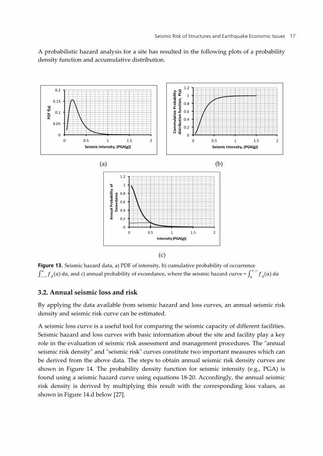
A probabilistic hazard analysis for a site has resulted in the following plots of a probability density function and accumulative distribution.

Figure 13. Seismic hazard data, a) PDF of intensity, b) cumulative probability of occurrence ( )−∞ , and c) annual probability of exceedance, where the seismic hazard curve = ( )+∞

3.2. Annual seismic loss and risk

By applying the data available from seismic hazard and loss curves, an annual seismic risk density and seismic risk curve can be estimated.

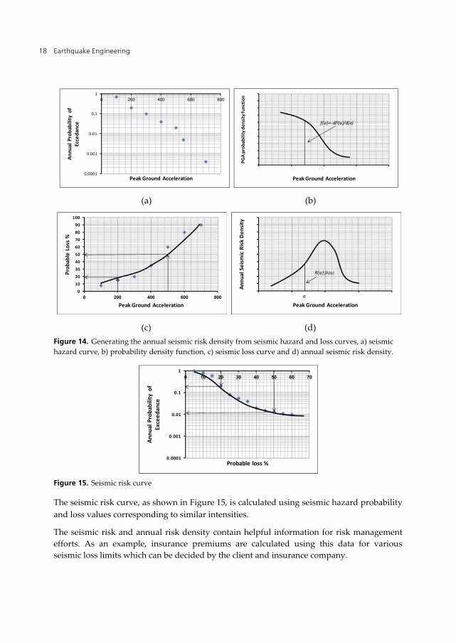
A seismic loss curve is a useful tool for comparing the seismic capacity of different facilities. Seismic hazard and loss curves with basic information about the site and facility play a key role in the evaluation of seismic risk assessment and management procedures. The "annual seismic risk density" and "seismic risk" curves constitute two important measures which can be derived from the above data. The steps to obtain annual seismic risk density curves are shown in Figure 14. The probability density function for seismic intensity (e.g., PGA) is found using a seismic hazard curve using equations 18-20. Accordingly, the annual seismic risk density is derived by multiplying this result with the corresponding loss values, as shown in Figure 14.d below [27].

(a) (b)

(c)

0

0.05

0.1

0.15

0.2

0 0.5 1 1.5 2

PDF

f(a)

Seismic Intensity, (PGA(g))

0

0.2

0.4

0.6

0.8

1

1.2

0 0.5 1 1.5 2

Com

mul

ativ

e Pr

obab

ility

di

strib

utio

n fu

nctio

n, P

(a)

Seismic Intensity, (PGA(g))

0

0.2

0.4

0.6

0.8

1

1.2

0 0.5 1 1.5 2

Annu

al P

roba

bilit

y of

Ex

ceed

ance

Intensity (PGA(g))


Figure 14. Generating the annual seismic risk density from seismic hazard and loss curves, a) seismic hazard curve, b) probability density function, c) seismic loss curve and d) annual seismic risk density.

Figure 15. Seismic risk curve

The seismic risk curve, as shown in Figure 15, is calculated using seismic hazard probability and loss values corresponding to similar intensities.

The seismic risk and annual risk density contain helpful information for risk management efforts. As an example, insurance premiums are calculated using this data for various seismic loss limits which can be decided by the client and insurance company.

(a) (b)

(c) (d)

0.0001

0.001

0.01

0.1

10 200 400 600 800

Annu

al P

roba

bilit

y of

Ec

ceda

nce

Peak Ground Acceleration

0

10

20

30

40

50

60

70

80

90

100

0 200 400 600 800

PGA

prob

abili

ty d

ensi

ty fu

nctio

n


f(a)=-dP(a)/d(a)

0

10

20

30

40

50

60

70

80

90

100

0 200 400 600 800

Prob

able

Los

s %


0

10

20

30

40

50

60

70

8090

100

0 200 400 600 800

Annu

al S

eism

ic Ri

sk D

ensi

ty

Peak Ground Accelerationa

R(a) fA(a)

0.0001

0.001

0.01

0.1

10 10 20 30 40 50 60 70

Annu

al P

roba

bilit

y of

Ex

ceed

ance

Probable loss %


4. Regional economic models

Perhaps the most widely used modelling framework is the Input-Output model. The method has been extensively discussed in the literature (for example, in [28-30]). The method is a linear model, which includes purchase and sales between sectors of an economy based on technical relations of production. The method specially focuses on the production interdependencies among the elements and, therefore, is applicable for efficiently exploring how damage in a party or sector may affect the output of the others. HAZUS has employed the model in its indirect loss estimation module [31].

Computable General Equilibrium (CGE) offers a multi-market simulation model based on the simultaneous optimization of behaviour of individual consumers and firms in response to price signals, subject to economic account balances and resource constraints. The nonlinear approach retains many of the advantages of the linear I-O methods and overcomes most of its disadvantages [32].

As the third alternative, econometric models are statistically estimated as simultaneous equation representations of the aggregate workings of an economy. A huge data collection is required for the model and the computation process is usually costly [33].

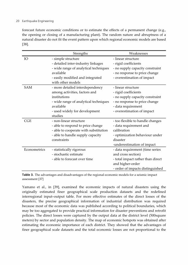
As another approach, Social Accounting Matrices (SAMs) have been utilized to examine the higher-order effects across different socio-economic agents, activities and factors. Cole, in [34-36], studied the subject using one of the variants of SAM. The SAM approach, like I-O models, has rigid coefficients and tends to provide upper bounds for estimates. On the other hand, the framework can derive the distributional impacts of a disaster in order to evaluate equity considerations for public policies against disasters. A summary of the advantages and disadvantages of the models mentioned has been presented in Table 3 [37].

The economic consequences of earthquakes due to the intensity of the event and the characteristics of the affected structures may be influential on a large-scale economy. As an example, the loss flowing from the March 2011 earthquake and tsunami in east Japan could amount to as much as $235 billion and the effects of the disaster will be felt in economies across East Asia [3]. To study how the damage to an economic sector of society may ripple into other sectors, regional economic models are employed. Several spatial economic models have been applied to study the impacts of disasters. Okuyama and Chang, in [30], summarized the experiences about the applications of the three main models - namely Input-Output, Social Accounting and Compatible General Equilibrium - to handle the impact of disaster on socio-economic systems, and comprehensively portrayed both their merits and drawbacks. However, they are based on a number of assumptions that are questionable in, for example, seismic catastrophes.

Studies have been recommended to address issues such as double-counting, the response of households and the evaluation of financial situations. According to the National Research Council, 'the core of the problem with the statistically based regional models is that the historical relationship, embodied in these models, is likely to be disrupted in a natural disaster. In short, regional economic models have been developed over time primarily to


forecast future economic conditions or to estimate the effects of a permanent change (e.g., the opening or closing of a manufacturing plant). The random nature and abruptness of a natural disaster do not fit the event pattern upon which regional economic models are based [38].

Strengths Weaknesses IO - simple structure

- detailed inter-industry linkages - wide range of analytical techniques available - easily modified and integrated with other models

- linear structure - rigid coefficients - no supply capacity constraint - no response to price change - overestimation of impact

SAM - more detailed interdependency among activities, factors and institutions - wide range of analytical techniques available - used widely for development studies

- linear structure - rigid coefficients - no supply capacity constraint - no response to price change - data requirement - overestimation of impact

CGE - non-linear structure - able to respond to price change - able to cooperate with substitution - able to handle supply capacity constraints

- too flexible to handle changes - data requirement and calibration - optimization behaviour under disaster -underestimation of impact

Econometrics - statistically rigorous - stochastic estimate - able to forecast over time

- data requirement (time series and cross section) - total impact rather than direct and higher-order - order of impacts distinguished

Table 3. The advantages and disadvantages of the regional economic models for a seismic impact assessment [37]

Yamano et al., in [39], examined the economic impacts of natural disasters using the originally estimated finer geographical scale production datasets and the redefined interregional input–output table. For more effective estimates of the direct losses of the disasters, the precise geographical information of industrial distribution was required because most of the economic data was published according to political boundaries, which may be too aggregated to provide practical information for disaster preventions and retrofit policies. The direct losses were captured by the output data at the district level (500square meters) by sector and population density. The map of economic hotspots was obtained after estimating the economic importance of each district. They showed that the advantages of finer geographical scale datasets and the total economic losses are not proportional to the


distributions of the population and industrial activities. In other words, the disaster prevention and retrofit policies have to consider the higher-order effects in order to reduce the total economic loss [39].

It has been shown that in having both virtues and limitations, these alternate I-O, CGE or econometric frameworks may be chosen according to various considerations, such as data collection/compilation, the expected output, research objectives and costs. Major impediments to analysing a disaster’s impact may involve issues related to data collection and estimation methodologies, the complex nature of a disaster’s impact, an inadequate national capacity to undertake impact assessments and the high frequency of natural disasters.

5. Conclusions

In this chapter, a summary of the methodology for performance-based earthquake engineering and its application in seismic loss estimation was reviewed. Describing the primary and secondary effects of earthquakes, it was mentioned that the loss estimation process for the direct loss estimation of structures consists of four steps, including hazard analysis, structural dynamics analysis, damage analysis and seismic loss analysis. EDPs, as the products of structural dynamic analysis, were explained and the methodologies’ seismic fragility curves were briefly introduced. Employing a probabilistic hazard analysis, the method for deriving the annual probability of seismic risk exceedance and seismic risk curves was presented. Considering the importance of both secondary effects and interactions between different sectors of an economy due to seismic loss, those regional economic models with common application in the evaluation of economic conditions after natural disasters (e.g., earthquakes) were mentioned.

Author details

Afshin Kalantari International Institute of Earthquake Engineering and Seismology, Iran

6. References

[1] The Third International Workshop on Earthquake and Megacities, Reducing Vulnerability, Increasing Sustainability of the World's Megacities. Shanghai, China, 2002.

[2] UNICEF, Sichuan Earthquake One Year Report. May 2009. [3] The recent earthquake and Tsunami in Japan: implications for East Asia, World Bank

East Asia and pacific Economic Update 2011, Vol. 1. [4] Financial Management of Earthquake Risk, Earthquake Engineering Research Institute

(EERI), May 2000.


[5] Bertero R. D. and Bertero V. V., Performance-based seismic engineering: the need for a reliable conceptual comprehensive approach, Earthquake Engineering and Structural Dynamics, 2002; 31, pp. 627–652.

[6] Dowrick D. J., Earthquake Risk Reduction. John Wiley & Sons Ltd, 2005. [7] Okuyama Y., Impact Estimation Methodology: Case Studies in: Global Facility for

Disaster Reduction and Recovery, www.gfdrr.org. [8] The Institute of Civil Engineers Megacities Overseas Development Administration,

Reducing Vulnerability to Natural Disasters. Thomas Telford Publications, 1995. [9] ATC-58 Structural and Structural Performance Products Team, ATC-58 Project Task

Report, Phase 3, Tasks 2.2 and 2.3, Engineering Demand Parameters for Structural Framing Systems, Applied Technology Council, 2004.

[10] ATC-58 Nonstructural Performance Products Team, ATC-58 Project Task Report, Phase 3, Task 2.3, Engineering Demand Parameters for Nonstructural Components, Applied Technology Council, 2004.

[11] Moehle J. P., A Framework for Performance-Based Earthquake Engineering. Proceedings, Tenth U.S.-Japan Workshop on Improvement of Building Seismic Design and Construction Practices, ATC-15-9 Report, Applied Technology Council, Redwood City, California, 2003.

[12] FEMA, 2000a, NEHRP Recommended Provisions for Seismic Regulations for Buildings and Other Structures, Part 1, Provisions, prepared by the Building Seismic Safety Council, published by the Federal Emergency Management Agency, Report No. FEMA 368, Washington, DC.

[13] FEMA, 2000b, NEHRP Recommended Provisions for Seismic Regulations for Buildings and Other Structures, Part 2, Commentary, prepared by the Building Seismic Safety Council, published by the Federal Emergency Management Agency, Report No. FEMA 369, Washington, DC.

[14] Williams M. S. and Sexsmith R. G., Seismic damage indices for concrete structures: a state-of the-art review. Earthquake Spectra, 1995, Volume 11, No. 2, pp. 319-349.

[15] Park Y. J. and Ang A. H.-S, Mechanistic seismic damage model for reinforced concrete. Journal of Structural Engineering, 1985, Vol. 111, No. 4, pp. 722-739.

[16] Powell G.H. and Allahabadi R., Seismic damage prediction by deterministic methods: concepts and procedures. Earthquake Engineering and Structural Dynamics, 1988, Vol. 16, pp. 719-734.

[17] Fajfar P., Equivalent ductility factors, taking into account low-cycle fatigue. Earthquake Engineering and Structural Dynamics, 1999, Vol. 21, pp. 837-848.

[18] Mehanny S. and Deierlein G. G., Assessing seismic performance of composite (RCS) and steel moment framed buildings, Proceedings, 12th World Conference on Earthquake Engineering, Auckland, New Zealand, 2000.

[19] Bozorgnia Y. and Bertero V. V., Damage spectra: characteristics and applications to seismic risk reduction. Journal of Structural Engineering, 2003, Vol. 129, No. 10, pp. 1330-1340.


[20] Sarabandi1 P., Pachakis D., King S. and Kiremidjian A., Empirical Fragility Functions from Recent, Earthquakes, 13WCEE, 13th World Conference on Earthquake Engineering, Vancouver, B.C., Canada, August 1-6, 2004, Paper No. 1211.

[21] Hwang H., Liu J. B. and Chiu Y., Seismic Fragility Analysis of Highway Bridges. Technical Report, MAEC RR-4 Project, Center for Earthquake Research and Information, The University of Memphis, 2001.

[22] Choi E., DesRoches R. and Nielson B., Seismic fragility of typical bridges in moderate seismic zones. Engineering Structures, 2004, 26, pp. 187–199.

[23] Padgett J. E and DesRoches R., Methodology for the development of analytical fragility curves for retrofitted bridges. Earthquake Engineering and Structural Dynamics, 2008, 37, pp. 1157–1174.

[24] Padgett J. E., Nielson B. G. and DesRoches R., Selection of optimal intensity measures in probabilistic seismic demand models of highway bridge portfolios, Earthquake Engineering and Structural Dynamics, 2008, 37, pp. 711–725.

[25] Bazzurro P. and Cornell C. A., Seismic hazard analysis for non-linear structures. I &2, ASCE Journal of Structural Engineering 1994; 120, 11, pp. 3320–3365.

[26] Earthquake Damage Evaluation Data for California, ATC 13, Applied Technology Council, Founded by Federal Emergency Management Agency, 1985.

[27] Seismic Risk Management of Civil Engineering Structures, Hoshiya M., Nakamura T. San Kai Do, 2002 (in Japanese).

[28] Cochrane H. C., Predicting the economic impacts of earthquakes. in: H.C. Cochrane, J. E. Haas and R. W. Kates (Eds) Social Science Perspectives on the Coming San Francisco Earthquakes—Economic Impact, Prediction, and Reconstruction, Natural Hazard Working Paper No.25, University of Colorado, Institute of Behavioural Sciences, 1974.

[29] Rose A. J., Benavides S. E., Chang P., Szczesniak P. and Lim D., The Regional Economic Impact of an Earthquake: Direct Effects of Electricity Lifeline Disruptions. Journal of Regional Science, 1997, 37, 3, pp. 437-458.

[30] Okuyama Y. and Chang S., (Editors), Modelling Spatial and Economic Impacts of Disasters, Springer, 2004.

[31] Federal Emergency Management Agency, Earthquake Loss Estimation Methodology (HAZUS). Washington, DC; National Institute of Building Science, 2001.

[32] Rose A. and Liao S. Y., Modelling regional economic resilience to disasters: a computable general equilibrium analysis of water service disruptions, Journal of Regional Science, 2005, 45, pp. 75-112.

[33] Rose A. and Guha G. S., Computable general equilibrium modelling of electric utility lifeline losses from earthquakes, in: Y. Okuyama and S. E. Chang, (Eds) Modelling Spatial and Economic Impacts of Disasters, 2004, pp. 119-141, Springer.

[34] Cole S., Lifeline and livelihood: a social accounting matrix approach to calamity preparedness, Journal of Contingencies and Crisis Management, 1995, 3, pp. 228-40.

[35] Cole S., Decision support for calamity preparedness: socioeconomic and interregional impacts, in M. Shinozuka, A. Rose and R. T. Eguchi, (Eds) Engineering and Socioeconomic Impacts of Earthquakes, 1998, pp. 125-153, Multidisciplinary Center for Earthquake Engineering Research.


[36] Cole S., Geohazards in social systems: an insurance matrix approach, in: Y. Okuyama and S.E. Chang (Eds) Modelling Spatial and Economic Impacts of Disasters, 2004, pp. 103-118, Springer.

[37] Okuyama Y., Critical review of methodologies on disaster impact estimation, Background Paper to the joint World Bank - UN Assessment on the Economics of Disaster Risk Reduction, 2009.

[38] National Research Council (Committee on assessing the cost of natural disasters, The impact of disasters, A framework for loss estimation. Washington, DC; National Academy Press, 1999.

[39] Yamano N. Kajitani Y. and Shumuta Y., Modelling the Regional Economic Loss of Natural Disasters: The Search for Economic Hotspots. Economic Systems Research, 2007, Volume 19, Issue 2, Special Issue: Economic Modelling for Disaster Impact Analysis, pp. 163-181.

Documents

Seismic Risk of Structures and the Economic Issues of