Seismic physical modeling II: VVAZ and AVAZ effects ... · Seismic physical modeling II: VVAZ and AVAZ effects observed on reflections from isolated HTI targets Joe Wong ABSTRACT

Physical modeling of marine surveys

CREWES Research Report — Volume 25 (2013) 1

Seismic physical modeling II: VVAZ and AVAZ effects observed on reflections from isolated HTI targets

Joe Wong

ABSTRACT

Seismic physical modeling was used to investigate VVAZ and AVAZ phenomena associated with targets having HTI anisotropy. Land-type surveys were carried out for a two-layer model consisting of an isotropic elastic layer overlying an HTI layer. Transmission and reflection seismograms from these land surveys exhibit clear evidence of VVAZ effects. In addition, 3D marine surveys were conducted over isolated HTI targets embedded in an isotropic slab using acquisition geometries designed to emphasize AVAZ effects of reflections from the HTI targets. An attribute based on constant-offset reflection amplitudes and another attribute showing lamination orientations were extracted from the 3D datasets. On maps of these attributes, clear anomalies occur at the true locations of the HTI targets.

INTRODUCTION

The University of Calgary Seismic Physical Modeling Facility is designed to enable investigators to easily carry out scaled-down 2D and 3D seismic surveys using ultrasonic transducers as sources and receivers. The facility consists of a precision 3D positioning subsystem, and a high-speed analogue-to-digital conversion subsystem. Both subsystems are controlled and coordinated by software running under a Windows operating system. The software records seismograms and stores them in SEGY files for post survey processing and analysis. In modeling, we typically will apply a scaling factor of 104 to convert model dimensions and times into real-world equivalents. This means that 1mm in a model represents 10m in the real world, and a model time of 1 microsecond represents 10 real-world milliseconds (in subsequent sections of this report, most dimensions and times will be expressed as real-world units). More information about the U of C Seismic Physical Modeling Facility may be found in a CSEG Recorder article by Wong et al. (2008a, 2008b; 2009).

Previous physical-modeling characterization of seismic anisotropy was done with transmission measurements through a single extensive HTI layer made up of Phenolic LE material, and with simulated marine reflection survey over a multi-layer model which included an HTI layer. Details and results for the previous investigation were presented by Mahmoudian et al. (2011, 2012). For the results reported here, we made transmission and reflection measurements on a two-layer structure consisting of an isotropic elastic Plexiglas layer overlying an HTI layer made up of Phenolic CE material. Both layers are homogeneous in their seismic properties. We also made reflection measurements in simulated 3D marine surveys conducted over a heterogeneous layer consisting of isolated HTI targets resembling hockey pucks embedded in an isotropic slab. Attributes extracted from the transmission and reflection seismograms exhibited clear evidence of VVAZ and AVAZ effects.

Wong

2 CREWES Research Report — Volume 25 (2013)

Plexiglas is a plastic with isotropic properties. It has P-wave velocity of 2750m/s, S-wave velocity of 1380m/s, and a density of 119 kg/m3.

Phenolic CE and Phenolic LE are composite laminated materials with very similar elastic properties. Slabs of Phenolic with thickness up to 104mm (4 inches) are manufactured by stacking many thin sheets of cloth on top of each other, and then saturating and bonding them together with an epoxy compound. The cloth sheets are woven from threads of cotton (CE) or linen (LE). For phenolic CE material, the threads are coarser than the threads for Phenolic LE, but the final macroscopic velocities are very similar. In the X-Y plane parallel to the laminations, the P-wave velocities are about 3450 m/s and 3550 m/s. In the Z-direction normal to the cloth sheets, the P wave velocity is roughly 15% lower at about 2800 m/s to 2900 m/s. Phenolic appears to be orthorhombic in its macroscopic seismic properties, but since the velocities in the XY plane are so close, we can consider it to be transversely isotropic with the symmetry axis perpendicular to the individual sheets, i.e., in the Z direction. Table 1 is a summary of the seismic velocities of the two materials taken from Cheadle et al. (1993) and Mahmoudian et al. (2011).

TABLE 1. Seismic velocities (m/s) and densities (kg/m3) of Phenolic CE and LE.

Phenolic Vpx Vpy Vpz Vsx Vsy Vsz Density

CE 3550 3450 2850 1600 1600 1600 1680

LE 3550 3450 2850 1600 1600 1600 1680

LAND-TYPE MEASUREMENTS USING A TWO-LAYER STRUCTURE

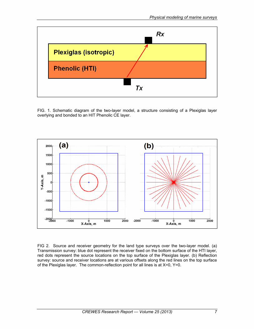
Figure 1 is a schematic diagram showing a structure consisting of a Plexiglas layer overlying bonded to the HIT phenolic CE layer. Both layers are about 490m thick, with lateral dimension of 3050m by 3050m. For our modeling experiments, the fast-velocity direction of the HTI layer was aligned with the X-axis of the modeling coordinate system. Two types of measurements were made to study the VVAZ behaviour of the two-layer model.

For the transmission measurements depicted on Figure 2(a), the receiver (RX) was fixed at the centre of the bottom surface of the HTI layer. The source (TX) was placed on the top surface of the Plexiglas layer on circles at azimuth angles that range from 0º to 360 º with 4º increments, measured counter-clockwise from the X-axis. Two sets of measurements were made, one each on the two circles shown with radius of 500m and 100m. These surveys simulated multi-azimuth VSP surveys with a downhole receiver fixed at a single depth.

Reflection measurements were made with the source and receiver transducers placed on the top surface of the acrylic layer. Common reflection point (CRP) gathers were acquired with the source receiver transducers placed along lines with azimuth angles of 0°, ±14°, ±27°, ±37°, ±45°, ±53°, ±63°, ±76° and 90°. Figure 2(b) shows the geometry of the azimuth-CRP reflection survey lines over the two-layer model.



For the transmission measurements, P-type (Panametrics V133) and S-type (Panametrics V156) ultrasonic transducers were used as receivers and sources. These transducers have 9 mm outside diameters; the diameters of their active elements are specified to be equal to 6.3mm. For the reflection experiments, Dynasen CA-1136 piezopins were use as the source and receive. The piezopins have outside diameters of 2.6mm and are 305mm long. In all the measurements, the transducers were placed in direct contact with the surfaces of the solid layers. Petroleum jelly was used to improve the transducer-to-solid coupling.

RESULTS FROM THE LAND SURVEYS

Transmission (VSP) survey

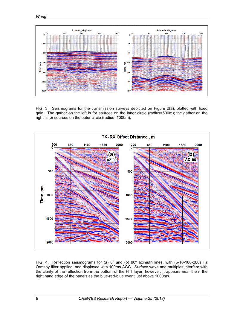
Figure 3 shows two azimuth gathers of transmission seismograms, with source locations on circles of radii equal to 500m and 1000m.

On the gather of seismograms for circle with 1000m radius, the direct P-wave arrivals occur at times near 500ms. Strong S-wave direct arrivals occur at times near 900ms. The P and S arrival times show a very distinct variation with azimuth. Minimum arrival times are indicative of the fast-velocity direction occur at angles of 0, 180, and 360 degrees. Maximum arrival times indicative of the slow-velocity direction and symmetry axis of the HTI layer occur at angles of 90 and 270 degrees. The direct arrival times can be converted to apparent velocities that exhibit VVAZ effects. The presence of VVAZ behaviour in the results of the modeled VSP survey reveals the presence of the HTI layer in the two-layer model.

First arrival peak-to-peak amplitudes also display variation with azimuth. Amplitude maxima and minima coincide with arrival time maxima and minima, respectively. The relative amplitudes at various azimuths are indicative of the relative transmission coefficients through the HTI/isotropic interface.

Azimuth-CRP reflection survey

Figure 4 shows CRP seismograms for two of the 37 lines that make up the full azimuth-CRP survey. The PP reflection of interest, i.e., from the bottom of the HTI layer, should begin at the 200m offset distance at about 670ms. Converted wave arrivals and random arrivals with no spatial coherence, caused by scattering within the HTI layer, obscure this reflection. However, it seems to become discernible just before 1000ms at the very far offsets. As yet, no extra processing and analysis has been done on the seismograms from the azimuth-CRP reflection survey.

MARINE 3D SURVEYS OVER THE “PUCK” MODEL

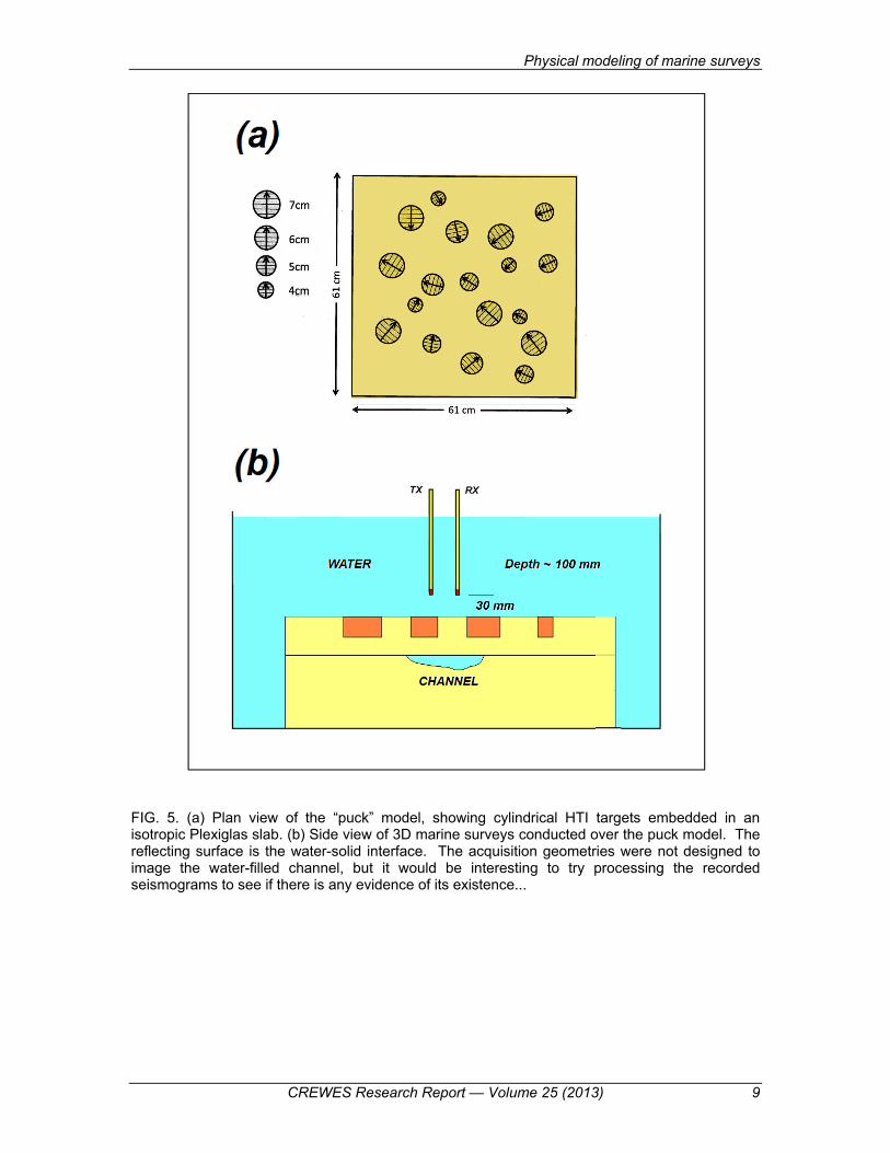
Figure 5(a) illustrates a model consisting of HTI cylinders embedded in a Plexiglas plastic slab. The scaled thickness of the slab is nominally 508m, and has lateral dimension of 5900m by 5900m. The HTI cylinders, which resemble hockey pucks, are 254m thick and have diameters that vary from 200m to 400m. This heterogeneous layer was immersed in about 1300m of water. Single piezopin transducers (Dynasen CA-1136) were used as a source and receiver for data acquisition. The active tips of the transducers were raised 300 m above the water-solid interface. Because the water–air

Wong


interface is about 1000m above the active tips, reflections from this interface arrive at times much later than the reflections of interest, i.e., those from the water-solid interface. By setting up the acquisition geometry in this way, we ensure that no multiples from the air-water surface interfere with the reflected arrivals of interest. Figure 5(b) is a side view of the general setup of the marine 3D surveys.

The origin (0, 0) of the modeling coordinate system was set at the very center of the Plexiglas slab.

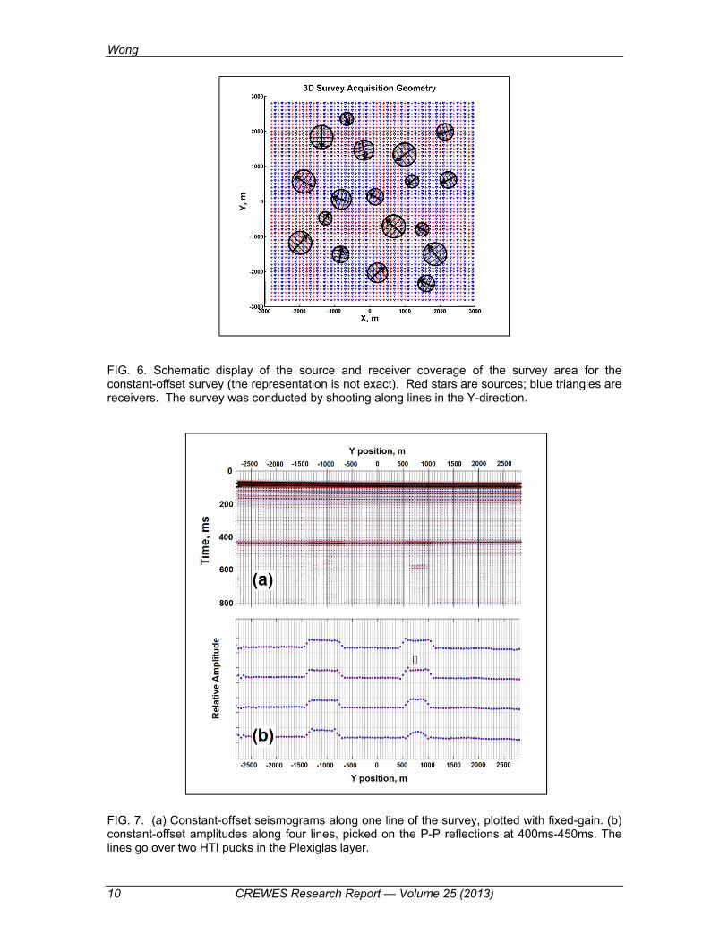
Two surveys were conducted an over area enclosed by the square bounded by X and Y limits of -2700m and 2700m. The first survey was done using with a constant 100m source-receiver X offset, with a single seismograms recorded at every location on a grid with intervals of Δx = Δy = 50m. The locations of sources and receivers on the gridded area over the “puck” model are shown schematically on Figure 6. The constant-offset survey produced data for creating maps of reflection amplitudes from the fluid-solid interface. We note that the constant-offset amplitudes are equivalent to brute-stack amplitudes produced by a much more time-consuming standard 3D survey.

The second survey was done over the same area, but with a grid spacing Δx = Δy = 100m. Every grid point is the centre of a circle with radius of 200m. We placed sources and receivers on opposite ends of diameters on the circle with azimuth angles (relative to the X-axis) in the range -90° to +90° at 5° intervals. This procedure produced 37 seismograms for every point on the survey grid, and generated CRP (common-reflection point) amplitudes information for the water-solid interface as a function of azimuth.

ANALYSIS AND RESULTS OF THE 3D MARINE SURVEYS

Marine constant-offset survey

Figure 7(a) is fixed-gain plot of seismograms on a line from the constant-offset survey. The line goes over two HTI pucks in the Plexiglas layer. P-P reflections from the water-solid interface occur at times between 400ms and 500ms. We see a faint but discernible increase in the reflection amplitudes at positions near -100m and 900m. There are definite anomalies displayed on Figure 7(b), where relative reflection amplitudes along four adjacent lines are plotted. The seismic lines go over two isolated HTI targets. The lateral extents of the anomalies are related to the sizes of the targets. Such reflection amplitudes for every grid point along every survey line can be picked and mapped.

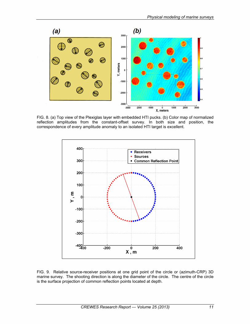
Figure 8(a) shows the top view of the Plexiglas layer with embedded HTI pucks. Figure 8(b) is the map of the observed normalized reflection amplitudes. Every high-amplitude feature on this map corresponds to an HTI puck in the Plexiglas layer.

Marine circle survey

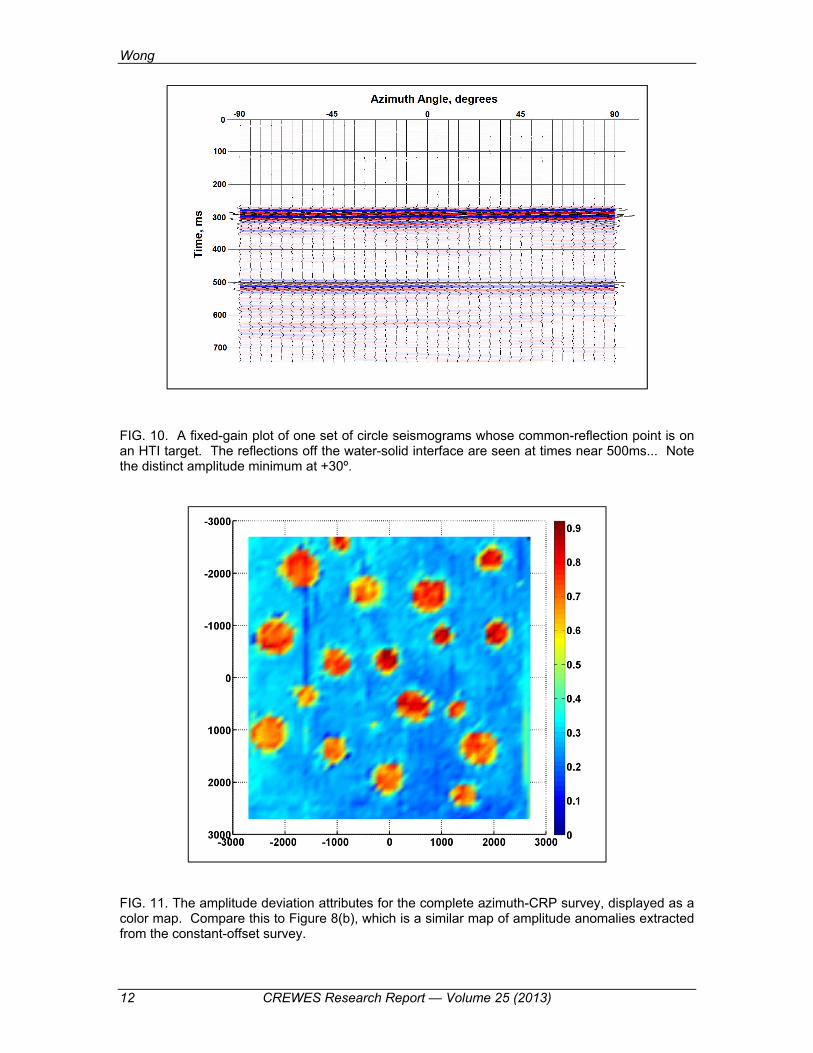
Figure 9 is a summary plot of the acquisition procedure used in the circle survey. At each of the 3025 grid points, CRP seismograms were recorded with source and receiver positions on the circle shown. Figure 10 is a fixed-gain plot of one set of circle seismograms whose common-reflection point is on an HTI target, and the relevant event from the water-solid interface is seen at times of 400ms to 600ms. The variation of amplitudes with azimuth angle for CRP reflections off the HTI target is obvious.



Reflection amplitudes from the water-solid interface as a function of azimuth can be picked for every grid point on the 3D survey. From this information, we extracted two attributes. The first attribute is the difference between maximum and minimum reflection amplitudes at every grid point. This attribute is displayed on Figure 11, and it maps the positions and lateral extents of the HTI pucks in much the same way as the constant-offset amplitude information did on Figure 7, but at lower resolution since the grid spacing is larger by a factor of two.

The second attribute, which we call the HTI anisotropy attribute, enables us to create a map that displays the lamination or “fracture” direction of each HTI target. For every grid point, we picked the angle with minimum reflection amplitude. The HTI attribute is calculated as the direction cosines of the minimum-amplitude angle scaled by the first attribute (i.e., the maximum-to-minimum amplitude difference).

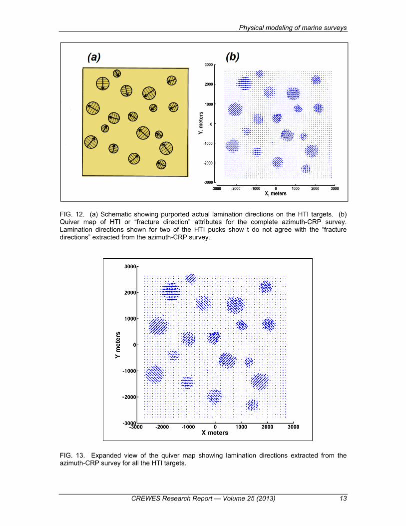
HTI attributes for the complete survey are displayed as a quiver map on Figure 12(b). We see that the arrows on the quiver map align in the directions of HTI target laminations shown on Figure 12(a) in every case except for two. For the two exceptions, visual examination of the actual solid model shows that Figure 12(a) is in error, and their lamination directions agree with those indicated by the quiver map arrows.

According to the theory of HTI velocity anisotropy for fractured or finely-layered geological media, the fast-velocity direction is identical to the fracture direction or direction of bedding, while the slow-velocity direction is normal to the fracture direction or bedding. The arrow directions on the quiver map correspond quite well with the actual lamination directions of the Phenolic pucks.

CONCLUSION

We made transmission and reflection measurements on a two-layer model consisting of an isotropic elastic Plexiglas layer overlying an HTI layer constructed of Phenolic CE material. Both layers are homogeneous in their seismic properties. These measurements simulated land surveys in that the source and receiver transducers made direct contact with surfaces of solid layers. The transmission measurements yielded seismograms exhibiting VVAZ behaviour that revealed the presence of the HTI layer.

We also conducted a simulated 3D marine surveys conducted over a heterogeneous layer consisting of isolated HTI targets embedded in an isotropic slab. Using acquisition geometries designed to highlight seismic AVAZ effects, physical-modeled high-resolution 3D surveys produced azimuth-CRP reflection seismograms from which HTI anisotropy attributes were extracted. A map of the HTI anisotropy attributes clearly delineated the locations of the HTI targets and revealed their lamination directions.

ACKNOWLEDGEMENT

We thank the industrial sponsors of CREWES and the Natural Sciences and Engineering Research Council of Canada for supporting this research.

Wong


REFERENCES

Cheadle, S. P., Brown, R. J., and Lawton, D. C., 1991, Orthorhombic anisotropy: a physical seismic modeling study: Geophysics, 56, 1603-1613.

Mahmoudian, F., Margrave, G.F., Wong, J., and Russell, B., 2011, AVAZ inversion for anisotropy

parameters of a fractured medium: a physical modeling study, CREWES Research Report, 23, 74.1-74.28.

Mahmoudian, F., Margrave, G.F., Daley, P.F., and Wong, J., 2012, Estimation of stiffness coefficients of

an orthorhombic physical model from group velocity measurements, CREWES Research Report, 24, 67.1-67.16.

Mahmoudian, F., 2013, Physical modeling and analysis of seismic data from a simulated fractured medium,

PhD. Dissertation, University of Calgary. Wong, J., Hall, K., Gallant, E., and Bertram, M., 2008a, Mechanical and electronic design for the U of C

Seismic Physical Modeling Facility, CREWES Research Report 20, 18.1-18.17. Wong, J., Hall, K., and Maier, R., 2008b, Control and acquisition software for the U of C Seismic Physical

Modeling Facility, CREWES Research Report 20, 19.1-19.14. Wong, J., Hall, K., Gallant, E., Maier, R., and Bertram, M., 2009, Seismic physical modeling at the

University of Calgary, CSEG Recorder, 36, 25-32.



FIG. 1. Schematic diagram of the two-layer model, a structure consisting of a Plexiglas layer overlying and bonded to an HIT Phenolic CE layer.

FIG 2. Source and receiver geometry for the land type surveys over the two-layer model. (a) Transmission survey: blue dot represent the receiver fixed on the bottom surface of the HTI layer, red dots represent the source locations on the top surface of the Plexiglas layer. (b) Reflection survey: source and receiver locations are at various offsets along the red lines on the top surface of the Plexiglas layer. The common-reflection point for all lines is at X=0, Y=0.

Wong


FIG. 3. Seismograms for the transmission surveys depicted on Figure 2(a), plotted with fixed gain. The gather on the left is for sources on the inner circle (radius=500m); the gather on the right is for sources on the outer circle (radius=1000m);

FIG. 4. Reflection seismograms for (a) 0º and (b) 90º azimuth lines, with (5-10-100-200) Hz Ormsby filter applied, and displayed with 100ms AGC. Surface wave and multiples interfere with the clarity of the reflection from the bottom of the HTI layer; however, it appears near the n the right hand edge of the panels as the blue-red-blue event just above 1000ms.



FIG. 5. (a) Plan view of the “puck” model, showing cylindrical HTI targets embedded in an isotropic Plexiglas slab. (b) Side view of 3D marine surveys conducted over the puck model. The reflecting surface is the water-solid interface. The acquisition geometries were not designed to image the water-filled channel, but it would be interesting to try processing the recorded seismograms to see if there is any evidence of its existence...

Wong


FIG. 6. Schematic display of the source and receiver coverage of the survey area for the constant-offset survey (the representation is not exact). Red stars are sources; blue triangles are receivers. The survey was conducted by shooting along lines in the Y-direction.

FIG. 7. (a) Constant-offset seismograms along one line of the survey, plotted with fixed-gain. (b) constant-offset amplitudes along four lines, picked on the P-P reflections at 400ms-450ms. The lines go over two HTI pucks in the Plexiglas layer.



FIG. 8. (a) Top view of the Plexiglas layer with embedded HTI pucks. (b) Color map of normalized reflection amplitudes from the constant-offset survey. In both size and position, the correspondence of every amplitude anomaly to an isolated HTI target is excellent.

FIG. 9. Relative source-receiver positions at one grid point of the circle or (azimuth-CRP) 3D marine survey. The shooting direction is along the diameter of the circle. The centre of the circle is the surface projection of common reflection points located at depth.

Wong


FIG. 10. A fixed-gain plot of one set of circle seismograms whose common-reflection point is on an HTI target. The reflections off the water-solid interface are seen at times near 500ms... Note the distinct amplitude minimum at +30º.

FIG. 11. The amplitude deviation attributes for the complete azimuth-CRP survey, displayed as a color map. Compare this to Figure 8(b), which is a similar map of amplitude anomalies extracted from the constant-offset survey.



FIG. 12. (a) Schematic showing purported actual lamination directions on the HTI targets. (b) Quiver map of HTI or “fracture direction” attributes for the complete azimuth-CRP survey. Lamination directions shown for two of the HTI pucks show t do not agree with the “fracture directions” extracted from the azimuth-CRP survey.

FIG. 13. Expanded view of the quiver map showing lamination directions extracted from the azimuth-CRP survey for all the HTI targets.

Documents

Seismic physical modeling II: VVAZ and AVAZ effects ... · Seismic physical modeling II: VVAZ and AVAZ effects observed on reflections from isolated HTI targets Joe Wong ABSTRACT