Seismic modelling of unconventional reservoirsMarco PerezApache Canada Ltd., Calgary, Alberta, Canada

Introduction

Unconventional resource development has become an exer-cise in determining where horizontal wells should be placedto maximize hydro-fracture efficiency. A large part of opti-mizing how the resource is developed requires under-standing the reservoir from both lithologic and rockproperties perspectives and correlating these with produc-tion data to infer frac efficiency. Given the variety of uncon-ventional plays in North America, it is important tounderstand the differences in rock properties so as to effec-tively map them seismically. Figure 1 shows backscatteredelectron images displaying the diversity in microstructurebeyond the differences in lithology.

Understanding the variations in terms of mineralogicalcomposition and microstructure requires an in depth model.With such a model, templates can be generated for interpre-tation of seismic attributes.

The following is an examination of two distinct rock physicsmodels and how they can be employed to generate seismicinterpretation templates. These templates can then be used inconjunction with inverted volumes of seismic attributes tomap lithologic and rock property variations. In addition,from the rock physics trends, AVO models are synthesized toevaluate potential offset dependent amplitude responses.

Two different rock physics models

The process begins with a comparison of two distinct rockphysics models. Each model will be reviewed, referencing

previous important works followed by suggesting potentialapplication to unconventional reservoirs. The first is a gran-ular model referred to as the modified Hertz-MindlinHashin-Shtrikman (HMHS) while the second, referred to asthe Non-Interacting Approximation (NIA) is an inclusionbased model which describes the number of pores and theirshapes as opposed to the grain to grain contacts.

The modified Hertz-Mindlin Hashin-Shtrikman (HMHS)

This model is a granular representation of a rock in that itassumes a random packing of spheres under hydrostaticcompression. Contact between spheres is used to estimatebulk and shear moduli in terms of normal and tangentialstiffness. The expressions for the dry bulk and shear moduli,known as the Hertz-Mindlin estimates, are given by (Dvorkinand Nur, 1996)

1.

2.

where n is the coordination number (number of graincontacts), f is the amount of porosity, x is a grain frictionalcoefficient (more on this later), and R is the grain radius. Thenormal and tangential stiffnesses are

3.

4.

where G and v are the shear modulus and Poisson’s ratio ofthe sphere. The variable a is the radius of the contact areabetween the two spheres and an estimate is given byHertz,1882 (Duffaut et. al, 2010),

5.

where FN is the confining force acting between the twospheres, given by

6.

and P is the effective hydrostatic confining pressure.

The scalar value of x varies between 0 and 1 where 0 impliesno friction between grains and 1 implies infinite friction.There are models that describe the variation of the parameterx. Duffaut et. al (2010) and Bachrach and Avseth (2008)studied the impact of the parameter and proposed non-linearand linear expressions, respectively, to model frictional vari-ations. Bachrach and Avseth (2008) also investigate the effectsof grain shape (round versus angular) with respect to thecontact radius and its influence on the bulk and shear moduli.

54 CSEG RECORDER April 2013

Continued on Page 55

Coordinated by Satinder Chopra / M

eghan Brown

FOCU

S AR

TICL

E

Figure 1. Backscattered electron image of 9 different North Americanunconventional plays (Curtis et. al 2010).

ϕπ

( )=

−K

n

RS

1

12dry N

ϕπ

( )=

−K

n

RS

1

12dry N

ϕπ

ξ( )( )=

−+G

n

RS S

1

20dry N T

ϕπ

ξ( )( )=

−+G

n

RS S

1

20dry N T

=−

SGa

v

4

1N

=−

SGa

v

4

1N

=−

SGa

v

8

2T

=−

SGa

v

8

2T

( )≈

−

aF R v

G

3 1

8

N

13

( )≈

−

aF R v

G

3 1

8

N

13

( )≈

−

aF R v

G

3 1

8

N

13

( )≈

−

aF R v

G

3 1

8

N

13

April 2013 CSEG RECORDER 55

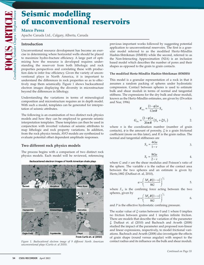
The Hertz-Mindlin estimate of K and G is used to describe a rockat the critical porosity end member. This end member is assumedto represent the starting point of rock formation. Any porositygreater than the critical porosity will result in grains in suspen-sion; not frame supported (Nur et. al, 1998). The Hashin-Shtrikman bounds are used to connect the critical porosity andthe solid, zero porosity end member to create upper and lowerlimits for porosity values between the end members. This tren isschematically shown in figure 1, along with the associated LMRrepresentation. These upper and lower bounds have been usedto describe cementing and sorting trends (Avseth et. al, 2010).

The Hashin-Shtrikman bounds describe lower and upper limitsto n-phase mixtures. The Hashin-Shtrikman bounds have theform (Mavko et. al, 2009)

7.

8.

where

9.

where Kn and Gn are the bulk and shear moduli of each phase, fnis the fractional quantity of each phase and G is the maximum(upper bound) or minimum (lower bound) shear modulus of allthe phases.

In the modified HMHS, which incorporates the critical porosityconcept, the bounds consist of two phases (n=2): the Hertz-Mindlin defined critical porosity and the mineral, zero porosityend member.

The Non-Interacting Approximation (NIA)

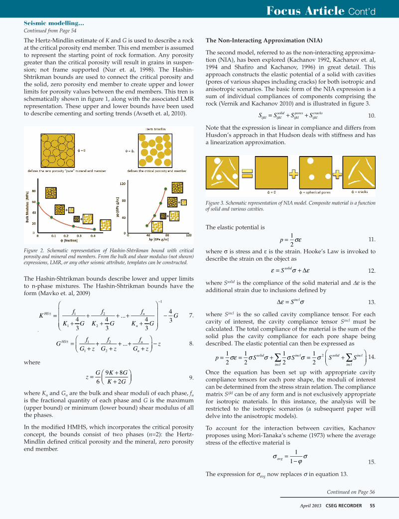
The second model, referred to as the non-interacting approxima-tion (NIA), has been explored (Kachanov 1992, Kachanov et. al,1994 and Shafiro and Kachanov, 1996) in great detail. Thisapproach constructs the elastic potential of a solid with cavities(pores of various shapes including cracks) for both isotropic andanisotropic scenarios. The basic form of the NIA expression is asum of individual compliances of components comprising therock (Vernik and Kachanov 2010) and is illustrated in figure 3.

10.

Note that the expression is linear in compliance and differs fromHusdon’s approach in that Hudson deals with stiffness and hasa linearization approximation.

The elastic potential is

11.

where s is stress and e is the strain. Hooke’s Law is invoked todescribe the strain on the object as

12.

where Ssolid is the compliance of the solid material and De is theadditional strain due to inclusions defined by

13.

where Sincl is the so called cavity compliance tensor. For eachcavity of interest, the cavity compliance tensor Sincl must becalculated. The total compliance of the material is the sum of thesolid plus the cavity compliance for each pore shape beingdescribed. The elastic potential can then be expressed as

14.

Once the equation has been set up with appropriate cavitycompliance tensors for each pore shape, the moduli of interestcan be determined from the stress strain relation. The compliancematrix Sijkl can be of any form and is not exclusively appropriatefor isotropic materials. In this instance, the analysis will berestricted to the isotropic scenarios (a subsequent paper willdelve into the anisotropic models).

To account for the interaction between cavities, Kachanovproposes using Mori-Tanaka’s scheme (1973) where the averagestress of the effective material is

15.

The expression for savg now replaces s in equation 13.

Focus Article Cont’d

Seismic modelling…Continued from Page 54

Continued on Page 56

Figure 2. Schematic representation of Hashin-Shtrikman bound with criticalporosity and mineral end members. From the bulk and shear modulus (not shown)expressions, LMR, or any other seismic attribute, templates can be constructed.

=+

++

+ ++

−±

−

K f

K G

f

K G

f

K G

G4

3

4

3

... 4

3

4

3

HS n

n

1

1

2

2

1

=+

++

+ ++

−±

−

Kf

K G

f

K G

f

K G

G4

3

4

3

...4

3

4

3

HS n

n

1

1

2

2

1

=+

++

+ ++

−±Gf

G z

f

G z

f

G zz...HS n

n

1

1

2

2

=+

++

+ ++

−±Gf

G z

f

G z

f

G zz...HS n

n

1

1

2

2

= + +S S S Sijkl ijkl

solid

ijkl

pores

ijkl

cracks

= + +S S S Sijkl ijkl

solid

ijkl

pores

ijkl

cracks

σε=p1

2

σε=p1

2

ε σ ε= + ∆Ssolid

ε σ ε= + ∆Ssolid

ε σ∆ = Sincl

ε σ∆ = Sincl

σϕ

σ=−1

1avg

σϕ

σ=−1

1avg

∑ ∑σε σ σ σ σ σ= = + = +

p S S S S1

2

1

2

1

2

1

2

solid incl

incl

solid incl

incl

2

∑ ∑σε σ σ σ σ σ= = + = +

p S S S S1

2

1

2

1

2

1

2

solid incl

incl

solid incl

incl

2

=+

+

zG K G

K G6

9 8

2

=+

+

zG K G

K G6

9 8

2

Figure 3. Schematic representation of NIA model. Composite material is a functionof solid and various cavities.

56 CSEG RECORDER April 2013

As per Vernik and Kachanov (2010), a spherical pores and crackdensity expression would be

16.

17.

where v is the Poisson’s ratio of the solid, f is porosity and n isthe crack density. Note that:

1. there is no stress dependence in this expression

2. porosity affects cracks, but cracks do not affect porosity.

Model comparison

The following will be an examination of the two different rockphysics models introduced. Specifically, the impact of pore shapeas described by the NIA model is investigated in an attempt torationalize differences between the granular and inclusionmodels. For the trends that follow, the rock is composed of 50%quartz, 25% clay and 25% limestone, representative of uncon-ventional reservoirs.

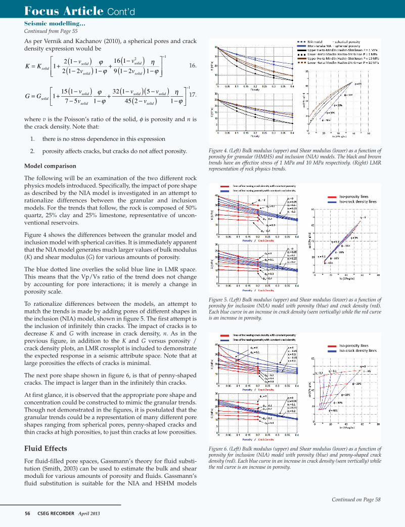
Figure 4 shows the differences between the granular model andinclusion model with spherical cavities. It is immediately apparentthat the NIA model generates much larger values of bulk modulus(K) and shear modulus (G) for various amounts of porosity.

The blue dotted line overlies the solid blue line in LMR space.This means that the Vp/Vs ratio of the trend does not change by accounting for pore interactions; it is merely a change inporosity scale.

To rationalize differences between the models, an attempt tomatch the trends is made by adding pores of different shapes inthe inclusion (NIA) model, shown in figure 5. The first attempt isthe inclusion of infinitely thin cracks. The impact of cracks is todecrease K and G with increase in crack density, n. As in theprevious figure, in addition to the K and G versus porosity /crack density plots, an LMR crossplot is included to demonstratethe expected response in a seismic attribute space. Note that atlarge porosities the effects of cracks is minimal.

The next pore shape shown in figure 6, is that of penny-shapedcracks. The impact is larger than in the infinitely thin cracks.

At first glance, it is observed that the appropriate pore shape andconcentration could be constructed to mimic the granular trends.Though not demonstrated in the figures, it is postulated that thegranular trends could be a representation of many different poreshapes ranging from spherical pores, penny-shaped cracks andthin cracks at high porosities, to just thin cracks at low porosities.

Fluid Effects

For fluid-filled pore spaces, Gassmann’s theory for fluid substi-tution (Smith, 2003) can be used to estimate the bulk and shearmoduli for various amounts of porosity and fluids. Gassmann’sfluid substitution is suitable for the NIA and HSHM models

Focus Article Cont’d

Seismic modelling…Continued from Page 55

Continued on Page 58

ϕϕ

ηϕ

( )( )( ) ( )= +

−− −

+−

− −

−

K Kv

v

v

v1

2 1

2 1 2 1

16 1

9 1 2 1solid

solid

solid

solid

solid

2 1

ϕϕ

ηϕ

( )( )( ) ( )= +

−− −

+−

− −

−

K Kv

v

v

v1

2 1

2 1 2 1

16 1

9 1 2 1solid

solid

solid

solid

solid

21

ϕϕ

ηϕ

( ) ( )( )( )= +

−− −

+− −

− −

−

G Gv

v

v v

v115 1

7 5 1

32 1 5

45 2 1solid

solid

solid

solid solid

solid

1

ϕϕ

ηϕ

( ) ( )( )( )= +

−− −

+− −

− −

−

G Gv

v

v v

v115 1

7 5 1

32 1 5

45 2 1solid

solid

solid

solid solid

solid

1

Figure 6. (Left) Bulk modulus (upper) and Shear modulus (lower) as a function ofporosity for inclusion (NIA) model with porosity (blue) and penny-shaped crackdensity (red). Each blue curve in an increase in crack density (seen vertically) whilethe red curve is an increase in porosity.

Figure 5. (Left) Bulk modulus (upper) and Shear modulus (lower) as a function ofporosity for inclusion (NIA) model with porosity (blue) and crack density (red).Each blue curve in an increase in crack density (seen vertically) while the red curveis an increase in porosity.

Figure 4. (Left) Bulk modulus (upper) and Shear modulus (lower) as a function ofporosity for granular (HMHS) and inclusion (NIA) models. The black and browntrends have an effective stress of 1 MPa and 10 MPa respectively. (Right) LMRrepresentation of rock physics trends.

58 CSEG RECORDER April 2013

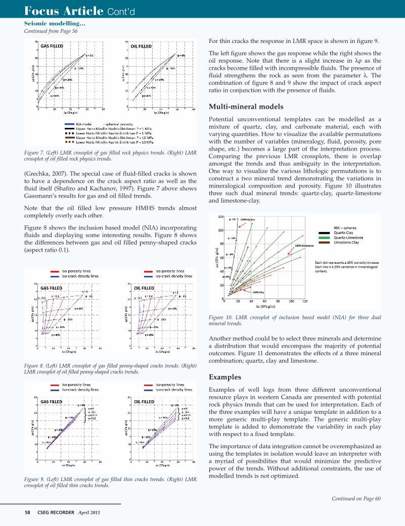
(Grechka, 2007). The special case of fluid-filled cracks is shownto have a dependence on the crack aspect ratio as well as thefluid itself (Shafiro and Kachanov, 1997). Figure 7 above showsGassmann’s results for gas and oil filled trends.

Note that the oil filled low pressure HMHS trends almostcompletely overly each other.

Figure 8 shows the inclusion based model (NIA) incorporatingfluids and displaying some interesting results. Figure 8 showsthe differences between gas and oil filled penny-shaped cracks(aspect ratio 0.1).

For thin cracks the response in LMR space is shown in figure 9.

The left figure shows the gas response while the right shows theoil response. Note that there is a slight increase in lr as thecracks become filled with incompressible fluids. The presence offluid strengthens the rock as seen from the parameter l. Thecombination of figure 8 and 9 show the impact of crack aspectratio in conjunction with the presence of fluids.

Multi-mineral models

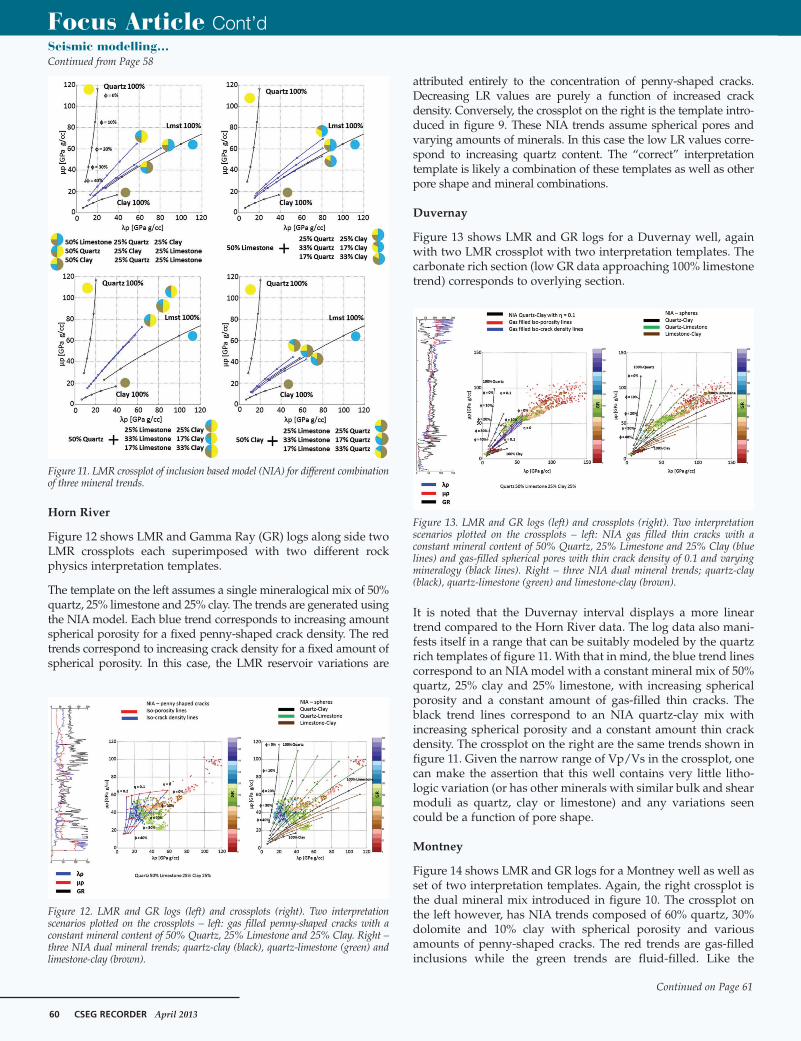
Potential unconventional templates can be modelled as amixture of quartz, clay, and carbonate material, each withvarying quantities. How to visualize the available permutationswith the number of variables (mineralogy, fluid, porosity, poreshape, etc.) becomes a large part of the interpretation process.Comparing the previous LMR crossplots, there is overlapamongst the trends and thus ambiguity in the interpretation.One way to visualize the various lithologic permutations is toconstruct a two mineral trend demonstrating the variations inmineralogical composition and porosity. Figure 10 illustratesthree such dual mineral trends: quartz-clay, quartz-limestoneand limestone-clay.

Another method could be to select three minerals and determinea distribution that would encompass the majority of potentialoutcomes. Figure 11 demonstrates the effects of a three mineralcombination; quartz, clay and limestone.

Examples

Examples of well logs from three different unconventionalresource plays in western Canada are presented with potentialrock physics trends that can be used for interpretation. Each ofthe three examples will have a unique template in addition to amore generic multi-play template. The generic multi-playtemplate is added to demonstrate the variability in each playwith respect to a fixed template.

The importance of data integration cannot be overemphasized asusing the templates in isolation would leave an interpreter witha myriad of possibilities that would minimize the predictivepower of the trends. Without additional constraints, the use ofmodelled trends is not optimized.

Focus Article Cont’d

Seismic modelling…Continued from Page 56

Continued on Page 60

Figure 10. LMR crossplot of inclusion based model (NIA) for three dualmineral trends.

Figure 9. (Left) LMR crossplot of gas filled thin cracks trends. (Right) LMRcrossplot of oil filled thin cracks trends.

Figure 8. (Left) LMR crossplot of gas filled penny-shaped cracks trends. (Right)LMR crossplot of oil filled penny-shaped cracks trends.

Figure 7. (Left) LMR crossplot of gas filled rock physics trends. (Right) LMRcrossplot of oil filled rock physics trends.

60 CSEG RECORDER April 2013

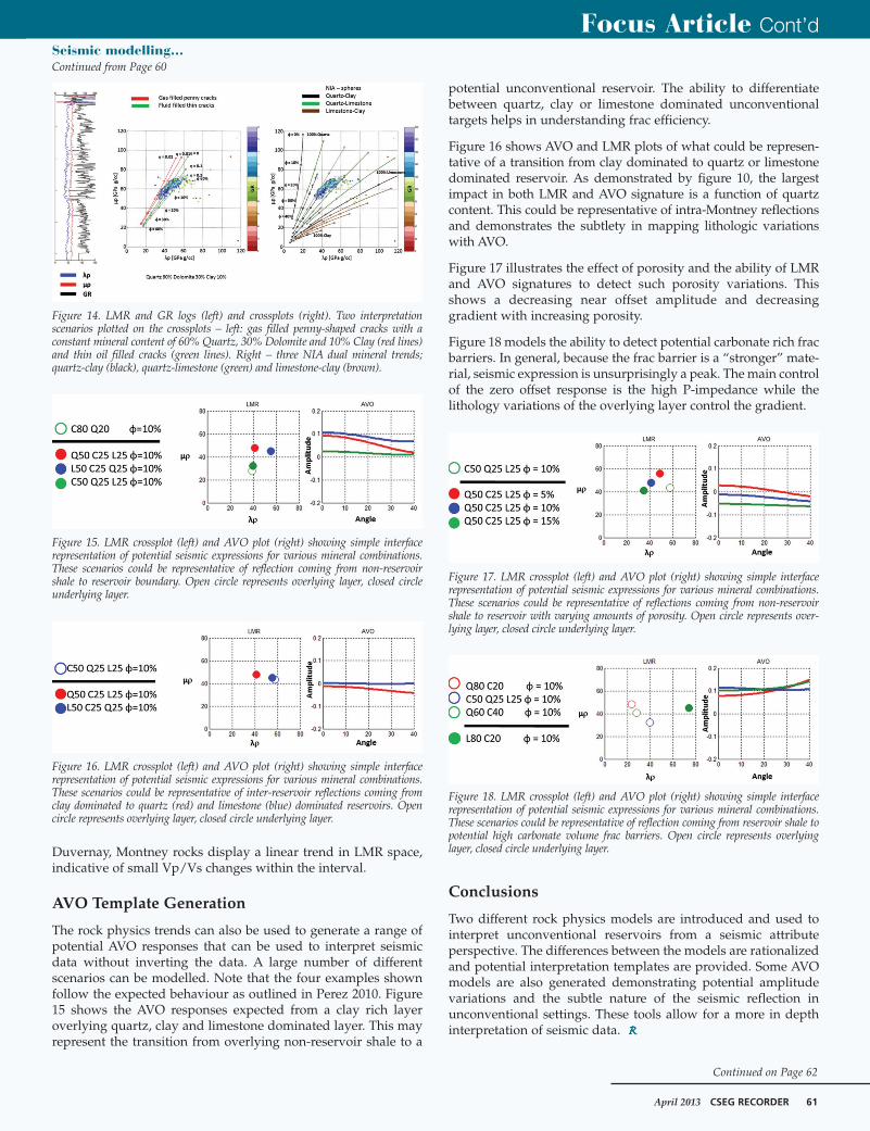
Horn River

Figure 12 shows LMR and Gamma Ray (GR) logs along side twoLMR crossplots each superimposed with two different rockphysics interpretation templates.

The template on the left assumes a single mineralogical mix of 50%quartz, 25% limestone and 25% clay. The trends are generated usingthe NIA model. Each blue trend corresponds to increasing amountspherical porosity for a fixed penny-shaped crack density. The redtrends correspond to increasing crack density for a fixed amount ofspherical porosity. In this case, the LMR reservoir variations are

attributed entirely to the concentration of penny-shaped cracks.Decreasing LR values are purely a function of increased crackdensity. Conversely, the crossplot on the right is the template intro-duced in figure 9. These NIA trends assume spherical pores andvarying amounts of minerals. In this case the low LR values corre-spond to increasing quartz content. The “correct” interpretationtemplate is likely a combination of these templates as well as otherpore shape and mineral combinations.

Duvernay

Figure 13 shows LMR and GR logs for a Duvernay well, againwith two LMR crossplot with two interpretation templates. Thecarbonate rich section (low GR data approaching 100% limestonetrend) corresponds to overlying section.

It is noted that the Duvernay interval displays a more lineartrend compared to the Horn River data. The log data also mani-fests itself in a range that can be suitably modeled by the quartzrich templates of figure 11. With that in mind, the blue trend linescorrespond to an NIA model with a constant mineral mix of 50%quartz, 25% clay and 25% limestone, with increasing sphericalporosity and a constant amount of gas-filled thin cracks. Theblack trend lines correspond to an NIA quartz-clay mix withincreasing spherical porosity and a constant amount thin crackdensity. The crossplot on the right are the same trends shown infigure 11. Given the narrow range of Vp/Vs in the crossplot, onecan make the assertion that this well contains very little litho-logic variation (or has other minerals with similar bulk and shearmoduli as quartz, clay or limestone) and any variations seencould be a function of pore shape.

Montney

Figure 14 shows LMR and GR logs for a Montney well as well asset of two interpretation templates. Again, the right crossplot isthe dual mineral mix introduced in figure 10. The crossplot onthe left however, has NIA trends composed of 60% quartz, 30%dolomite and 10% clay with spherical porosity and variousamounts of penny-shaped cracks. The red trends are gas-filledinclusions while the green trends are fluid-filled. Like the

Focus Article Cont’d

Seismic modelling…Continued from Page 58

Continued on Page 61

Figure 11. LMR crossplot of inclusion based model (NIA) for different combinationof three mineral trends.

Figure 12. LMR and GR logs (left) and crossplots (right). Two interpretationscenarios plotted on the crossplots – left: gas filled penny-shaped cracks with aconstant mineral content of 50% Quartz, 25% Limestone and 25% Clay. Right –three NIA dual mineral trends; quartz-clay (black), quartz-limestone (green) andlimestone-clay (brown).

Figure 13. LMR and GR logs (left) and crossplots (right). Two interpretationscenarios plotted on the crossplots – left: NIA gas filled thin cracks with aconstant mineral content of 50% Quartz, 25% Limestone and 25% Clay (bluelines) and gas-filled spherical pores with thin crack density of 0.1 and varyingmineralogy (black lines). Right – three NIA dual mineral trends; quartz-clay(black), quartz-limestone (green) and limestone-clay (brown).

April 2013 CSEG RECORDER 61

Duvernay, Montney rocks display a linear trend in LMR space,indicative of small Vp/Vs changes within the interval.

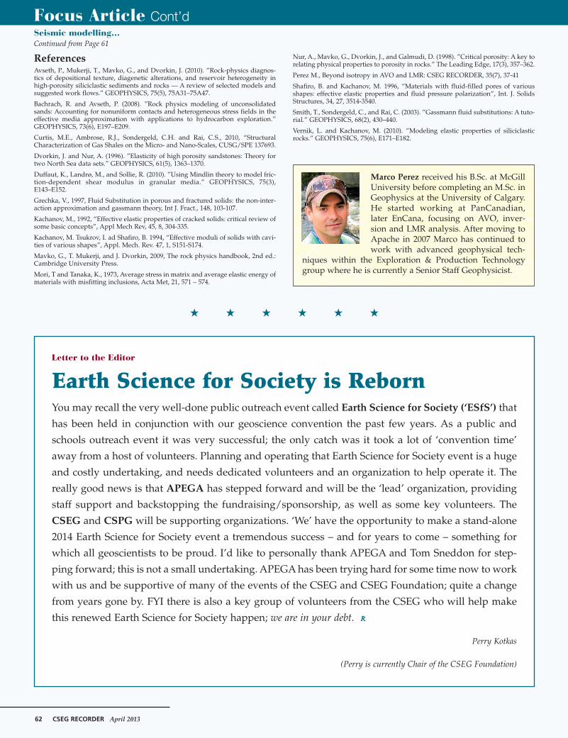
AVO Template Generation

The rock physics trends can also be used to generate a range ofpotential AVO responses that can be used to interpret seismicdata without inverting the data. A large number of differentscenarios can be modelled. Note that the four examples shownfollow the expected behaviour as outlined in Perez 2010. Figure15 shows the AVO responses expected from a clay rich layeroverlying quartz, clay and limestone dominated layer. This mayrepresent the transition from overlying non-reservoir shale to a

potential unconventional reservoir. The ability to differentiatebetween quartz, clay or limestone dominated unconventionaltargets helps in understanding frac efficiency.

Figure 16 shows AVO and LMR plots of what could be represen-tative of a transition from clay dominated to quartz or limestonedominated reservoir. As demonstrated by figure 10, the largestimpact in both LMR and AVO signature is a function of quartzcontent. This could be representative of intra-Montney reflectionsand demonstrates the subtlety in mapping lithologic variationswith AVO.

Figure 17 illustrates the effect of porosity and the ability of LMRand AVO signatures to detect such porosity variations. Thisshows a decreasing near offset amplitude and decreasinggradient with increasing porosity.

Figure 18 models the ability to detect potential carbonate rich fracbarriers. In general, because the frac barrier is a “stronger” mate-rial, seismic expression is unsurprisingly a peak. The main controlof the zero offset response is the high P-impedance while thelithology variations of the overlying layer control the gradient.

Conclusions

Two different rock physics models are introduced and used tointerpret unconventional reservoirs from a seismic attributeperspective. The differences between the models are rationalizedand potential interpretation templates are provided. Some AVOmodels are also generated demonstrating potential amplitudevariations and the subtle nature of the seismic reflection inunconventional settings. These tools allow for a more in depthinterpretation of seismic data. R

Focus Article Cont’d

Seismic modelling…Continued from Page 60

Continued on Page 62

Figure 14. LMR and GR logs (left) and crossplots (right). Two interpretationscenarios plotted on the crossplots – left: gas filled penny-shaped cracks with aconstant mineral content of 60% Quartz, 30% Dolomite and 10% Clay (red lines)and thin oil filled cracks (green lines). Right – three NIA dual mineral trends;quartz-clay (black), quartz-limestone (green) and limestone-clay (brown).

Figure 15. LMR crossplot (left) and AVO plot (right) showing simple interfacerepresentation of potential seismic expressions for various mineral combinations.These scenarios could be representative of reflection coming from non-reservoirshale to reservoir boundary. Open circle represents overlying layer, closed circleunderlying layer.

Figure 16. LMR crossplot (left) and AVO plot (right) showing simple interfacerepresentation of potential seismic expressions for various mineral combinations.These scenarios could be representative of inter-reservoir reflections coming fromclay dominated to quartz (red) and limestone (blue) dominated reservoirs. Opencircle represents overlying layer, closed circle underlying layer.

Figure 17. LMR crossplot (left) and AVO plot (right) showing simple interfacerepresentation of potential seismic expressions for various mineral combinations.These scenarios could be representative of reflections coming from non-reservoirshale to reservoir with varying amounts of porosity. Open circle represents over-lying layer, closed circle underlying layer.

Figure 18. LMR crossplot (left) and AVO plot (right) showing simple interfacerepresentation of potential seismic expressions for various mineral combinations.These scenarios could be representative of reflection coming from reservoir shale topotential high carbonate volume frac barriers. Open circle represents overlyinglayer, closed circle underlying layer.

Letter to the Editor

Earth Science for Society is RebornYou may recall the very well-done public outreach event called Earth Science for Society (‘ESfS’) that

has been held in conjunction with our geoscience convention the past few years. As a public and

schools outreach event it was very successful; the only catch was it took a lot of ‘convention time’

away from a host of volunteers. Planning and operating that Earth Science for Society event is a huge

and costly undertaking, and needs dedicated volunteers and an organization to help operate it. The

really good news is that APEGA has stepped forward and will be the ‘lead’ organization, providing

staff support and backstopping the fundraising/sponsorship, as well as some key volunteers. The

CSEG and CSPG will be supporting organizations. ‘We’ have the opportunity to make a stand-alone

2014 Earth Science for Society event a tremendous success – and for years to come – something for

which all geoscientists to be proud. I’d like to personally thank APEGA and Tom Sneddon for step-

ping forward; this is not a small undertaking. APEGA has been trying hard for some time now to work

with us and be supportive of many of the events of the CSEG and CSEG Foundation; quite a change

from years gone by. FYI there is also a key group of volunteers from the CSEG who will help make

this renewed Earth Science for Society happen; we are in your debt. R

Perry Kotkas

(Perry is currently Chair of the CSEG Foundation)

62 CSEG RECORDER April 2013

ReferencesAvseth, P., Mukerji, T., Mavko, G., and Dvorkin, J. (2010). ”Rock-physics diagnos-tics of depositional texture, diagenetic alterations, and reservoir heterogeneity inhigh-porosity siliciclastic sediments and rocks — A review of selected models andsuggested work flows.” GEOPHYSICS, 75(5), 75A31–75A47.

Bachrach, R. and Avseth, P. (2008). ”Rock physics modeling of unconsolidatedsands: Accounting for nonuniform contacts and heterogeneous stress fields in theeffective media approximation with applications to hydrocarbon exploration.”GEOPHYSICS, 73(6), E197–E209.

Curtis, M.E., Ambrose, R.J., Sondergeld, C.H. and Rai, C.S., 2010, “StructuralCharacterization of Gas Shales on the Micro- and Nano-Scales, CUSG/SPE 137693.

Dvorkin, J. and Nur, A. (1996). ”Elasticity of high�porosity sandstones: Theory fortwo North Sea data sets.” GEOPHYSICS, 61(5), 1363–1370.

Duffaut, K., Landrø, M., and Sollie, R. (2010). ”Using Mindlin theory to model fric-tion-dependent shear modulus in granular media.” GEOPHYSICS, 75(3),E143–E152.

Grechka, V., 1997, Fluid Substitution in porous and fractured solids: the non-inter-action approximation and gassmann theory, Int J. Fract., 148, 103-107.

Kachanov, M., 1992, “Effective elastic properties of cracked solids: critical review ofsome basic concepts”, Appl Mech Rev, 45, 8, 304-335.

Kachanov, M. Tsukrov, I. ad Shafiro, B. 1994, “Effective moduli of solids with cavi-ties of various shapes”, Appl. Mech. Rev. 47, 1, S151-S174.

Mavko, G., T. Mukerji, and J. Dvorkin, 2009, The rock physics handbook, 2nd ed.:Cambridge University Press.

Mori, T and Tanaka, K., 1973, Average stress in matrix and average elastic energy ofmaterials with misfitting inclusions, Acta Met, 21, 571 – 574.

Nur, A., Mavko, G., Dvorkin, J., and Galmudi, D. (1998). ”Critical porosity: A key torelating physical properties to porosity in rocks.” The Leading Edge, 17(3), 357–362.

Perez M., Beyond isotropy in AVO and LMR: CSEG RECORDER, 35(7), 37-41

Shafiro, B. and Kachanov, M. 1996, “Materials with fluid-filled pores of variousshapes: effective elastic properties and fluid pressure polarization”, Int. J. SolidsStructures, 34, 27, 3514-3540.

Smith, T., Sondergeld, C., and Rai, C. (2003). ”Gassmann fluid substitutions: A tuto-rial.” GEOPHYSICS, 68(2), 430–440.

Vernik, L. and Kachanov, M. (2010). ”Modeling elastic properties of siliciclasticrocks.” GEOPHYSICS, 75(6), E171–E182.

Focus Article Cont’d

Seismic modelling…Continued from Page 61

Marco Perez received his B.Sc. at McGillUniversity before completing an M.Sc. inGeophysics at the University of Calgary.He started working at PanCanadian,later EnCana, focusing on AVO, inver-sion and LMR analysis. After moving toApache in 2007 Marco has continued towork with advanced geophysical tech-

niques within the Exploration & Production Technologygroup where he is currently a Senior Staff Geophysicist.

★ ★ ★ ★ ★ ★