1

Seismic fragility curves for caisson-type quay walls

Joana Fernandes Chouriço

Department of Civil Engineering and Architecture (DECivil), Instituto Superior Técnico,

University of Lisbon

December 2015

Abstract: Port structures, including quay walls, have been damaged by earthquakes over the past

few years. The derivation of fragility curves is found to be very important for quantifying the

vulnerability of such structures. This study proposes fragility curves derived from two-dimensional

numerical simulations using FLAC 2D software. A set of soil profiles were used that fit the ground

types B, C and D defined by Eurocode 8. The seismic action was introduced using records of

earthquakes with a magnitude greater than 5,5. The quay wall was 10 m high and 10 m wide, while

the foundations were 20 m thick. The lower boundary of the model was absorbent. To evaluate

structural damage, 4 levels were defined based on standard horizontal displacement at the top of

the wall together with tilting.

Keywords: earthquakes, fragility curves, FLAC 2D, quay walls, caissons

1. Introduction

Port structures play an important role in international shipping, including the import and export of

goods and tourism. The consequences of an earthquake in port structures can be devastating, with

not only structural but also socio-economic repercussions. An example is the earthquake that occurred

in Japan in 1995 and which affected the port of Kobe, causing a loss of nearly 50% of the annual

income [1]. In most countries, international trade is predominantly done through seaports. It is

therefore imperative to reduce the vulnerability of quay walls.

This work derives fragility curves for use as a tool for studying the seismic vulnerability of port gravity

type structures, in a broad range of ground types.

2. Calibration of the numerical model

The FLAC 2D software was used to simulate the seismic behavior of a caisson type quay wall. This is

a program based on a finite difference method for simulating soil-structure interaction taking into

account the deformations and nonlinear soil behavior under cyclic loading.

2.1. 1D wave propagation

The propagation of shear waves was simulated using a soil column with linear elastic behavior in

order to evaluate the response of the soil to an action introduced at the outcrop. The vertical

boundaries were assumed to behave as free field boundaries, restricted in the horizontal direction in

order to simulate shear waves and, at the base, quiet boundaries were used to simulate the elastic

half-space. The transfer function between the base of the deposit and the surface was computed and

with the analytical solution for 1D shear wave propagation in a visco-elastic layer.

2

0

5

10

15

20

25

30

0 5 10 15 20

|H (w

)|

f [Hz]

Teórico ξ=2% Strata ξ=2% FLAC ξ=2%

Figure 2.1 - Transfer function of the calibration

model

Table 2.1 - Soil properties adopted for the soil

deposit

[kN/m3]

[MPa]

[MPa]

[m/s]

Table 2.2 - Soil properties adopted for half-space

[kN/m3]

[MPa]

[MPa]

[m/s]

2.2. Simulation of soil cyclic behavior

A one-zone element sample calibration was therefore

performed (Figure 2.2). The cyclic behavior of soils was

simulated using the Mohr-Coulomb non-linear elastic

perfectly plastic constitutive soil model, owing to its

relative simplicity and reduced number of parameters

(Table 2.3). The Mohr-Coulomb linear elastic perfectly

plastic constitutive soil model was also used in order to

assess a comparative analysis of the responses.

The Ishibashi and Zhang curves were chosen as a reference to simulate the strain-dependent

stiffness degradation of soil and damping coefficient curves.

Table 2.3 - Soil properties adopted

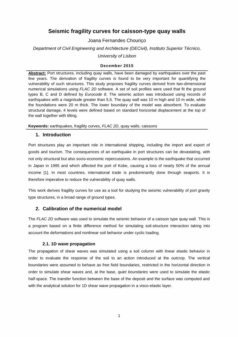
For this purpose the Ishibashi and Zhang curves were selected, considering IP=20 and p'=100 kPa

(Figure 2.4). The stress-strain relationship for different load levels is presented in Figure 2.3.

a) b) c)

Figure 2.3 - Stress-strain relationship for different load levels applied to a) b) c)

-20

-15

-10

-5

0

5

10

15

20

-2 -1 0 1 2 3 4 5 6

τ xy

[k

Pa

]

ϒ [%]

-20

-15

-10

-5

0

5

10

15

20

-2 -1 0 1 2 3 4 5 6

τ xy

[kP

a]

ϒ [%]

-20

-15

-10

-5

0

5

10

15

20

-2 -1 0 1 2 3 4 5 6

τ xy

[k

Pa

]

ϒ [%]

Figure 2.2 - Geometry adopted in modeling

3

0

10

20

30

40

50

60

70

0

0,1

0,2

0,3

0,4

0,5

0,6

0,7

0,8

0,9

1

0,0001 0,001 0,01 0,1 1 10

ξ [%]

G/G

0

ϒ [%]

Clays PI=20 G/G0 FLAC FLAC Curve theoretical ξ ξ FLAC

Although the shear stiffness degradation

curve (Figure 2.4) is penalized, both the

damping and the shear stiffness degradation

curves seem to correctly describe the non-

linearity of the soil.

2.3. 2D numerical model

In this section, the 2D numerical model to simulate soil-quay wall interaction is analyzed.

2.3.1. Geometry and material properties

The numerical modeling was performed assuming that the quay wall has 10 m high and 10 m wide.

The quay wall foundation soil has 20 m thick. The boundary conditions included free field boundaries

laterally applied together with absorbent boundaries applied at the base (Figure 2.5).

Figure 2.5 – Geometry and boundary conditions

The soil behavior was assumed to behave like the Mohr Coulomb non-linear elastic perfectly plastic

model, while the quay wall behavior was assumed to be linear elastic (Table 2.4).

Table 2.4 – Soil properties

Parameters Quay Wall Supported Soil Foundations Half-Space

1920

- 45

Figure 2.4 - Stiffness degradation and damping coefficient curves for clays with PI=20 and p´=100kPa

4

2.3.2. Gravity action

To simulate the tensions existing

in the model before the seismic

action, a static analysis

considering only the effect of

gravity was carried out. Figure

2.6 shows the initial in-situ

vertical total distribution stresses

generated.

2.3.3. Input seismic loading

A seismic action (Figure 2.7), recorded in the

Friuli earthquake, Italy, scaled to obtain PGAs of

0,05g, 0,4g and 0,8g, was then introduced. These

three levels of seismic intensity were chosen to

exhibit the behavior of the soil in three possible

behavior ranges: from very small to small

deformations, small to medium deformations and

large deformations, respectively.

2.3.4. Results

It can be clearly observed that the structure

suffers horizontal displacement as well as rotation

(Figure 2.8). The evolution in horizontal and

vertical displacements as well as the rotation

during the seismic action is shown in Figure 2.9

and Figure 2.10.

a) b) c)

Figure 2.9 - Displacement evolution during seismic action at point A of the quay wall for a) PGA = 0.05g; b) PGA

= 0.4g c) PGA = 0.8g

Figure 2.6 –initial in-situ vertical total distribution stresses

FLAC (Version 7.00)

LEGEND

12-Oct-15 10:43

step 50064

-5.556E+00 <x< 1.056E+02

-6.056E+01 <y< 5.056E+01

Grid plot

0 2E 1

YY-stress contours

-5.40E+05

-4.80E+05

-4.20E+05

-3.60E+05

-3.00E+05

-2.40E+05

-1.80E+05

-1.20E+05

-6.00E+04

0.00E+00

Contour interval= 6.00E+04

Extrap. by averaging -5.000

-3.000

-1.000

1.000

3.000

(*10 1̂)

0.100 0.300 0.500 0.700 0.900

(*10 2̂)

JOB TITLE : Campo de tensoes verticais [Pa]

FLAC (Version 7.00)

LEGEND

12-Oct-15 10:43

step 50064

-5.556E+00 <x< 1.056E+02

-6.056E+01 <y< 5.056E+01

Grid plot

0 2E 1

YY-stress contours

-5.40E+05

-4.80E+05

-4.20E+05

-3.60E+05

-3.00E+05

-2.40E+05

-1.80E+05

-1.20E+05

-6.00E+04

0.00E+00

Contour interval= 6.00E+04

Extrap. by averaging -5.000

-3.000

-1.000

1.000

3.000

(*10 1̂)

0.100 0.300 0.500 0.700 0.900

(*10 2̂)

JOB TITLE : Campo de tensoes verticais [Pa]

Figure 2.7 – Input seismic action

-0,3

-0,25

-0,2

-0,15

-0,1

-0,05

0

0,05

0 1 2 3 4 5 6

Dis

pla

ce

me

nt

[m]

t [s]Horizontal Vertical

-0,3

-0,25

-0,2

-0,15

-0,1

-0,05

0

0,05

0 1 2 3 4 5 6

Dis

pla

ce

me

nt

[m]

t [s]Horizontal Vertical

-0,3

-0,25

-0,2

-0,15

-0,1

-0,05

0

0,05

0 1 2 3 4 5 6

Dis

pla

ce

me

nt

[m]

t [s]Horizontal Vertical

Figure 2.8 - Deformed mesh at the end of the analysis for PGA=0,4g

5

a) b) c)

Figure 2.10 – Quay wall rotation for a) ; b) ; c)

There is a clear increase in both horizontal and vertical displacement (Figure 2.9) and rotation (Figure

2.10) of the quay wall with an increasingly stronger seismic action.

3. Fragility curves

Since the most common deformation modes found in rigid support structures are sliding, tilting and

settlement, the parameters used to define the minimum requirements for each level of damage (EDP's

- Engineering Demand Parameters) are linked to these modes. This study adopted the methodology

proposed in SYNER-G [1] to obtain fragility curves.

The International Navigation Association (PIANC 2001) [2] defines four damage levels (Degrees I-IV)

based on the degree of normalized residual horizontal displacement (d/H) together with any residual

tilting towards the sea (ϴ) (Table 3.1).

Table 3.1 – Definition of damage states for gravity quay walls (PIANC, 2001)

Damage levels, Degree I Degree II Degree III Degree IV

EDPs d/H <1,5%** 1,5% a 5% 5% a 10% > 10%

ϴ [ᵒ] < 3ᵒ 3ᵒ a 5ᵒ 5ᵒ a 8ᵒ > 8ᵒ

The lognormal cumulative probability distribution is used to define the fragility curves (1). These

curves demonstrate the probability of exceedance of a certain level of damage, previously established,

and are defined by:

(1)

Where: is the probability of exceeding a certain level of damage, dsi; Φ is the lognormal cumulative

distribution function; IM is the seismic motion intensity measurement; is the limit median value of

necessary to cause a certain level of damage, dsi; and

(2) is the total lognormal standard

deviation describing the overall uncertainty associated with each fragility curve, modeled by the

combination of the following sources of uncertainty: level of damage,

, response and bearing

capacity of the structure, and seismic movement,

.

(2)

-0,9

-0,8

-0,7

-0,6

-0,5

-0,4

-0,3

-0,2

-0,1

0

0,1

0 1 2 3 4 5 6

Ro

taç

ão

[ᵒ]

t [s]

-0,9

-0,8

-0,7

-0,6

-0,5

-0,4

-0,3

-0,2

-0,1

0

0,1

0 1 2 3 4 5 6

Ro

taç

ão

[ᵒ]

t [s]

-0,9

-0,8

-0,7

-0,6

-0,5

-0,4

-0,3

-0,2

-0,1

0

0,1

0 1 2 3 4 5 6

Ro

taç

ão

[ᵒ]

t [s]

6

The uncertainty associated with the definition of

damage states,

, is set equal to 0,4 while the

uncertainty due to the capacity , , is assigned equal to

0,3 [1].

A linear regression analysis was used to estimate the

parameters (lognormal standard deviation) and

(Figure 3.1).

3.1. Numerical model adopted

The geometry of the gravity quay wall was identical to the configuration adopted for the calibration 2D

model (Figure 2.5 in section 2.3.1) with the addition of a load to simulate the hydrostatic behavior.

The estimated horizontal displacements of the quay wall are strongly influenced not only by the type of

soil involved in the analysis, but also by the stiffness profile variation according to depth. Ignoring the

increase in stiffness variation with depth would thus translate into an inaccurate estimation of soil

displacements. The model was therefore divided into 5m thickness layers (Figure 3.2).

Figure 3.2 - Geometry and mesh of the model adopted in FLAC

To cover a broad range of ground types, defined in Eurocode 8, the Vs and Cu combination profiles

shown in Figure 3.3, which cover Eurocode 8 ground types B to D, were modeled.

a) b)

Figure 3.3 – Combinations of clay soils adopted a) S wave velocity profiles b) Cu profiles

Figure 3.1 – Example of a simple linear regression

to estimate the parameters and [4]

-20

-15

-10

-5

0

5

10

0 200 400 600 800

Pro

f. [m

]

Vs [m/s]

B-B C-B D-B C-C D-C D-D

-20

-15

-10

-5

0

5

10

0 200 400 600 800 1000

Pro

f. [m

]

Cu [kPa]

B-B C-B D-B C-C D-C D-D

7

40 records were applied to each Vs profile [3], where the value of the peak horizontal acceleration,

PHA, recorded corresponded to the respective type of foundation soil. These records were obtained at

different stations with different epicenters, hypocenters, magnitudes, duration, tectonic environment

and frequency content. The online European data seismic action platform, ESD, was used and

seismic records with a PHA varying between 0,9 to 7,85 m/s2 and magnitudes above 5,5 were

selected, aiming to include the variability inherent to seismic motion.

3.2. Sensitivity analysis

Most of the fragility curves available in the literature define the IM as the PHA. This parameter can be

obtained almost immediately from an accelerogram and for this reason it is often used in evaluating

the damage induced in a structure. In this analysis, the PGA recorded at the ground surface was used

as IM as well as Ia.

3.2.1. Variation effect of the supported soil

This section assesses the effect of supported soil, while keeping the soil foundation characteristics, in

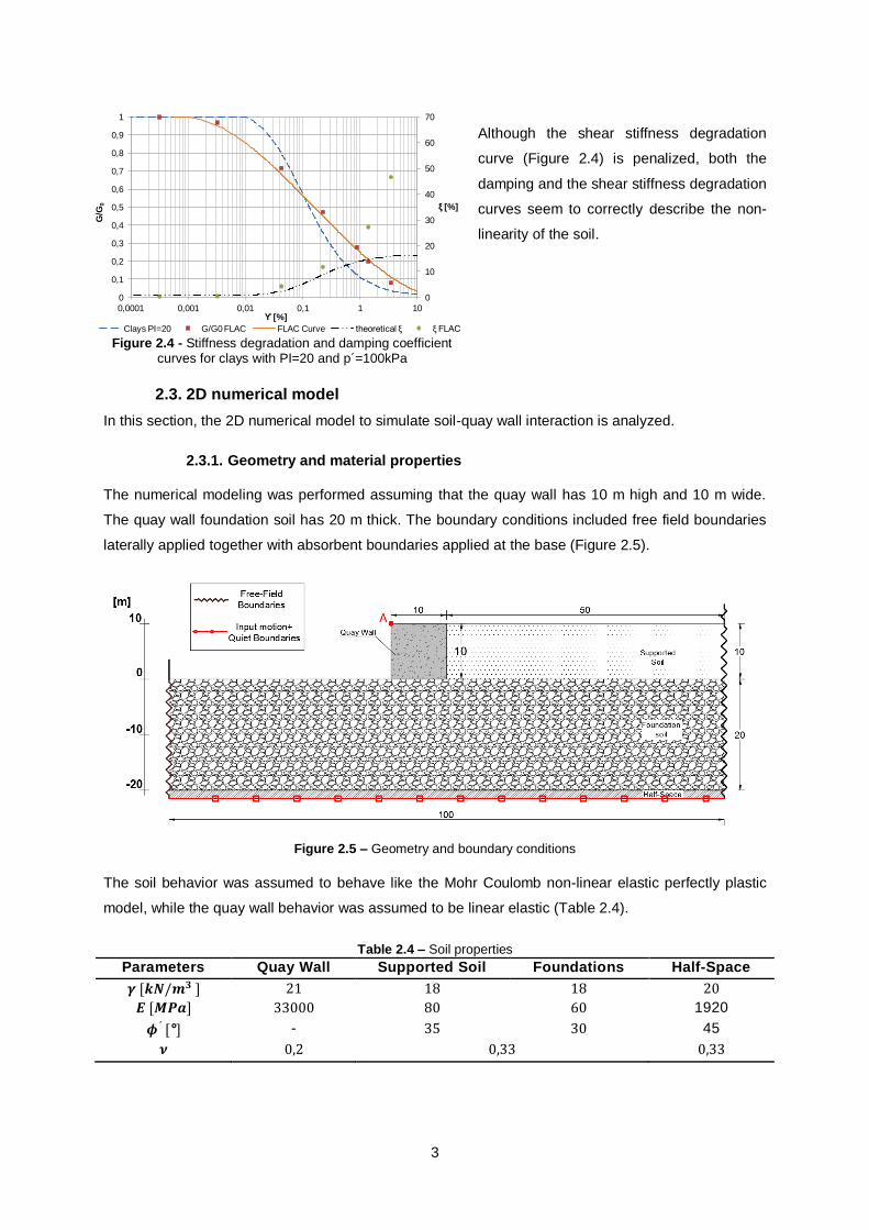
the fragility curve behavior. Figure 3.4 compares the effect of supported soil types C and D, with

foundation soil type C, using as IM parameter PGA and Ia.

a) b)

Figure 3.4 - Comparison of fragility curves considering EDP's HRND (d/H) for seismic combination SScSFc and SSdSFc as a function of a) PGA b) Ia

The decrease in the supported soil strength parameters, which causes an increase in displacements

at the top of the wall, is reflected in the curves, with an increasing likelihood of a certain level of

damage being exceeded.

3.2.2. Variation effect of the foundation soil

The deformation at the base of the quay wall is directly related to the stiffness of the foundation soil. In

this respect, Figure 3.5 presents the effect of the variability of the properties of the foundation layer

while maintaining the features of the supported soil.

0

0,2

0,4

0,6

0,8

1

0 0,1 0,2 0,3 0,4 0,5 0,6 0,7 0,8 0,9 1

Pf(

ds≥d

si|IM

)

PGA (g)

Degree I SScSFc Degree II SScSFc Degree III SScSFc

Degree I SSdSFc Degree II SSdSFc Degree III SSdSFc

0

0,2

0,4

0,6

0,8

1

0 1 2 3 4 5 6

Pf(

ds≥d

si|IM

)

Ia (m/s)

Degree I SScSFc Degree II SScSFc Degree III SScSFc

Degree I SSdSFc Degree II SSdSFc Degree III SSdSFc

8

a) b)

Figure 3.5 - Comparison of fragility curves considering EDP's HRND (d/H) for seismic combination SSdSFb, SSdSFc and SSdSFd as a function of a) PGA b) Ia

It can be noted that the foundation soil has a greater influence on the seismic response of the quay

wall than the supported soil. Comparing the combination in both figures (Figure 3.4 and Figure 3.5), it

can be seen that a decrease in the strength of foundation soil has a higher impact on the fragility

curves, with an increased probability of damage.

3.2.3. Comparison between displacement and rotation found

The comparison between the HRND and the rotation of the quay wall is illustrated in Figure 3.6.

a) b)

Figure 3.6 - Comparison of fragility curves considering EDP's HRND (d/H) and rotation (ϴ) for seismic combination SSdSFd as a function of a) PGA b) Ia

It can be seen that slipping prevails over quay wall rotation. The slip resistance is provided by soil

deformation at the wall base. Consequently, by reducing the strength parameters of the layer on which

the wall is based on, an increase in displacements can be expected.

3.3. Fragility curves

To validate the fragility curves obtained, the fragility curves found in SYNER-G [1] (Figure 3.7), namely

the curves obtained by Kakderi & Pitilaki (2010) [4] for H ≤10m and Vs = 500m/s (Type B) and Vs =

250m/s (Type C), were used. The combinations used to obtain the fragility curves for soil type C have

Vs,30 of 263 m/s, 265 m/s and 195 m/s.

0

0,2

0,4

0,6

0,8

1

0 0,1 0,2 0,3 0,4 0,5 0,6 0,7 0,8 0,9 1

Pf(

ds≥d

si|IM

)

PGA (g)

Grau I SSdSFb

Grau II SSdSFb

Grau III SSdSFb

Grau I SSdSFc

Grau II SSdSFc

Grau III SSdSFc

Grau I SSdSFd

Grau II SSdSFd

Grau III SSdSFd

0

0,2

0,4

0,6

0,8

1

0 1 2 3 4 5 6

Pf(

ds≥d

si|I

M)

Ia(m/s)

Grau I SSdSFb

Grau II SSdSFb

Grau III SSdSFb

Grau I SSdSFc

Grau II SSdSFc

Grau I SSdSFd

Grau II SSdSFd

0

0,2

0,4

0,6

0,8

1

0 0,1 0,2 0,3 0,4 0,5 0,6 0,7 0,8 0,9 1

Pf(

ds≥d

si|IM

)

PGA (g)

Degree I (d/H) Degree II (d/H) Degree III (d/H)

Degree I ϴ Degree II ϴ Degree III ϴ

0

0,2

0,4

0,6

0,8

1

0 1 2 3 4 5 6

Pf(

ds≥d

si|I

M)

Ia (m/s)

Degree I (d/H) Degree II (d/H) Degree III (d/H)

Degree I ϴ Degree II ϴ Degree III ϴ

9

a) b)

Figure 3.7 - Comparison of proposed fragility curves with those of Kakderi & Pitilakis (2010) [4] for soil type a) B

b) C

A large difference between the curves can be observed. There could be several reasons behind the

differences observed. To highlight a few: in addition to different geotechnical characteristics, the

seismic actions of Kakderi & Pitilakis (2010) [4] were scaled up, so that in the assessment of the

variability of magnitude there was lower scatter. The author also uses quay wall geometric

relationships B/H<1, resulting in higher horizontal displacements as a result of the walls rotation,

reflected in a higher probability of damage.

4. Conclusions and future perspectives

This study is dedicated to a seismic response analysis of a caisson-type quay wall based on two-

dimensional numerical simulation using the FLAC 2D program.

40 seismic records for different ground types were used as the input motion and residual horizontal

normalized displacement and rotation were computed to be used as EDPs for deriving fragility curves.

The damage levels proposed by PIANC were adopted. In the sensitivity study, it was concluded that:

the decrease in the strength of the supported soil, while maintaining the same type of foundation soil,

caused an increase in displacement and rotation, reflected in an increased likelihood of damage; the

foundation soil, while maintaining the same supported soil, had a greater influence on the dynamic

behavior of the quay wall than the supported soil; horizontal displacements generated higher levels of

damage than rotation; the rotation of the wall was negligible for soil foundations with soil types B and

C, while a higher likelihood of damage for soil type D was found.

From the fragility curves obtained for soil profiles B, C and D it can be concluded that the seismic

performance of the quay wall with clay soil types B and C is associated with lower damage, while clay

soil type D has a higher probability of damage.

Based on this work, it is proposed that future research should concentrate on: an analysis of sandy

soils including the generation of pore pressures in order to assess the behavior of a quay wall during

the possible occurrence of liquefaction; given the high dependence of the progress of fragility curves

on variability, more seismic actions should be used in the analysis; incorporation of hydrodynamic

behavior.

0

0,1

0,2

0,3

0,4

0,5

0,6

0,7

0,8

0,9

1

0 0,1 0,2 0,3 0,4 0,5 0,6 0,7 0,8 0,9 1

Pf(

ds≥d

si|IM

si)

PGA (g)

Degree I

Degree II

Degree III

Degree I Kakderi&Pitilakis

Degree II Kakderi&Pitilakis

0

0,1

0,2

0,3

0,4

0,5

0,6

0,7

0,8

0,9

1

0 0,1 0,2 0,3 0,4 0,5 0,6 0,7 0,8 0,9 1

Pf(d

s≥d

si|IM

si)

PGA (g)

Degree I

Degree II

Degree III

Degree I Kakderi&Pitilakis

Degree II Kakderi&Pitilakis

Degree III Kakderi&Pitilakis

10

Acknowledgements

This work was undertaken as a thesis to obtain a Masters degree in Civil Engineering at the Instituto

Superior Técnico, University of Lisbon, under the guidance of Professor Rui Pedro Carrilho Gomes.

References

[1] “Guidelines for deriving seismic fragility functions of elements at risk: Buildings, lifelines,

transportation networks and critical facilities - SYNER-G Reference Report 4,” European Union,

Luxembourg, 2013.

[2] PIANC, Seismic Design Guidelines for Port Structures, International Navigation Association, 2000.

[3] “European Soil Database (ESDB),” [Online]. Available: http://esdac.jrc.ec.europa.eu/.

[4] K. Kakderi e K. Pitilakis, “Seismic Analysis And Fragility Curves Of Gravity Waterfront Structures,”

em Fifth International Conference on Recent Advances in Geotechnical Earthquake Engineering

and Soil Dynamics, San Diego, California, 2010.

[5] S. Argyroudis, A. M. Kaynia e K. Pitilakis, “Development of fragility functions for geotechnical

constructions: Application to cantilever retaining walls,” Soil Dynamics and Earthquake

Engineering, vol. 50, pp. 106-116, 2013.