Seismic Drift Control and Building Periods EDWARD J. TEAL

General parameters of seismic drift control were discussed by the author in a 1975 article titled "Seismic Drift Control Criteria" in the AISC Engineering Journal. ^ However, the confusion which still exists concerning building periods and drift control, particularly in relation to code seismic design, indicates that these subjects deserve more attention. Building period governs the behavior of structures when they are subjected to earthquake ground motions, even when the dynamic response of the structure is forced far into the inelastic range during some of the strong motion. Drift, or distortion, really governs the performance of a building in terms of damage both to the structural frame and to non-frame elements. The designer needs to have a good understanding of the factors affecting these subjects. Knowing the limiting parameters is therefore important.

The 1976 Uniform Building Code (UBC) is probably the first code (and the only present code) to set a drift limit. Since designers are inclined to take code limits as design criteria, it is important to know what this limit provides. However, drift must always be associated with the force causing the drift, so the code specified forces and the dy­namic forces generated by probable maximum earthquake ground motions should both be considered in conjunction with drift. In another Engineering Journal article by the author, "Seismic Design Practice for Steel Buildings",^ only the code minimum requirements were considered, because that was the stated limit of scope for the article. This paper will attempt to give the designer a better understanding of drift control parameters so that he can use his own criteria as well as the code minimum requirements.

For those not fully familiar with the 1976 UBC seismic criteria, it is necessary to first briefly review the code force formula which must be used with the code drift control. The seismic design lateral force (shear) at the base of a building is given by a coefficient times the total weight of the building. In formula terms, V = CpW. The equivalent lateral force design coefficient, Cp, given in the 1976 UBC, is directly related to four factors:

Edward / . Teal is a Consulting Structural Engineer, Seismic Engineering Associates, Ltd., Los Angeles, Calif.

1. The zone seismicity factor, Z has values of 1.0, 0.5, or 0.25.

2. The frame factor, K, a force modifier (for stress cal­culations) for different frame inelastic response characteristics, has values of 1.33, 1.0, 0.80, or 0.67.

3. The importance factor, /, provides a multiplier of 1.5 for certain emergency important buildings.

4. The site response factor is a modifier 5, varying from 1.0 to 1.5, which is intended to provide for dynamic response amplification when the period of vibration of the building is close to that of the site.

The coefficient Cp is set at a value of Vis, or 0.067, when the four modifiers and the building period are all equal to unity. The effect of the building period on the dynamic response to earthquake ground motions is set by the factor 1 / A / T . When the constants Z, K, and / are all equal to 1, the code design seismic force coefficient is given by Cp = S/\ 5 A / T . This is not the anticipated maximum dynamic response to ground motions probable for the building site, but is an empirical design equivalent lateral force coeffi­cient.

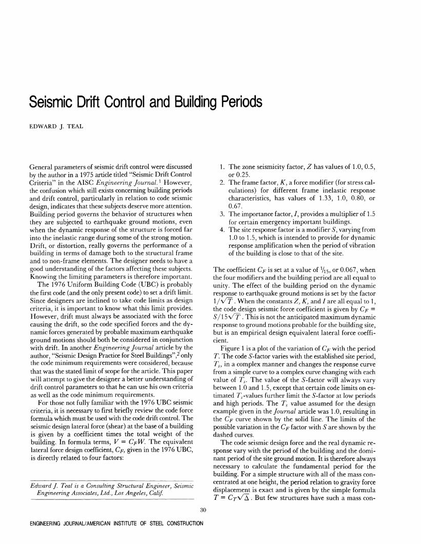
Figure 1 is a plot of the variation of Cp with the period T. The code 5-factor varies with the established site period, Ts, in a complex manner and changes the response curve from a simple curve to a complex curve changing with each value of 7" . The value of the 5-factor will always vary between 1.0 and 1.5, except that certain code limits on es­timated 7"^-values further limit the ^'-factor at low periods and high periods. The Ts value assumed for the design example given in the Journal article was 1.0, resulting in the Cp curve shown by the solid line. The limits of the possible variation in the Cp factor with S are shown by the dashed curves.

The code seismic design force and the real dynamic re­sponse vary with the period of the building and the domi­nant period of the site ground motion. It is therefore always necessary to calculate the fundamental period for the building. For a simple structure with all of the mass con­centrated at one height, the period relation to gravity force displacement is exact and is given by the simple formula T = C T - A / ^ . But few structures have such a mass con-

30

ENGINEERING JOURNAL/AMERICAN INSTITUTE OF STEEL CONSTRUCTION

o

0) o O

if)

a> (/) o

CD

0.14

hA\ kA\v \ \ > .

\ \ x \^y ^ v N

\ N \ ,

^^Min . Cp /

X^^ /

V ^ A" ^S=I .O

/ - T s = 1-0 '

- r = 1.5

0.033

Period T

Figure 1

centration, so exact period calculation for most structures depends on the exact deflected shape of the structure and is therefore complex. However, it is found that the period can be directly related to the square root of the maximum displacement under gravity force, just as for a single mass sytem. Also, feasible and practical design for most buildings limits the variation in deflected shapes to a fairly narrow band. It is found that the maximum displacement is by far the dominant variable, not the deflected shape. The period formula for buildings therefore can also be given by the formula T = CT^^^ , where CT is a variable depending on the deflected shape, but with narrow limits. A value for CT of 0.25 is a good approximation for most buildings when the displacement is computed for the code force dis­tribution. When the displacement is computed for the code force or a force coefficient Cp (always a fraction of gravity acceleration), the period formula becomes T =

CT^^X^7C~F-We are not really concerned with maximum displace­

ment, however. What we are concerned with is distortion as measured by the ratio of the story displacement to the story height. We can relate story distortion (drift) to the maximum building displacement and thereby derive a period formula related to a building drift coefficient. The building drift coefficient 0 will be close to the story drift coefficient if the building is tightly designed to control drift. The period formula can then be given as 7" = CWSH/CF-

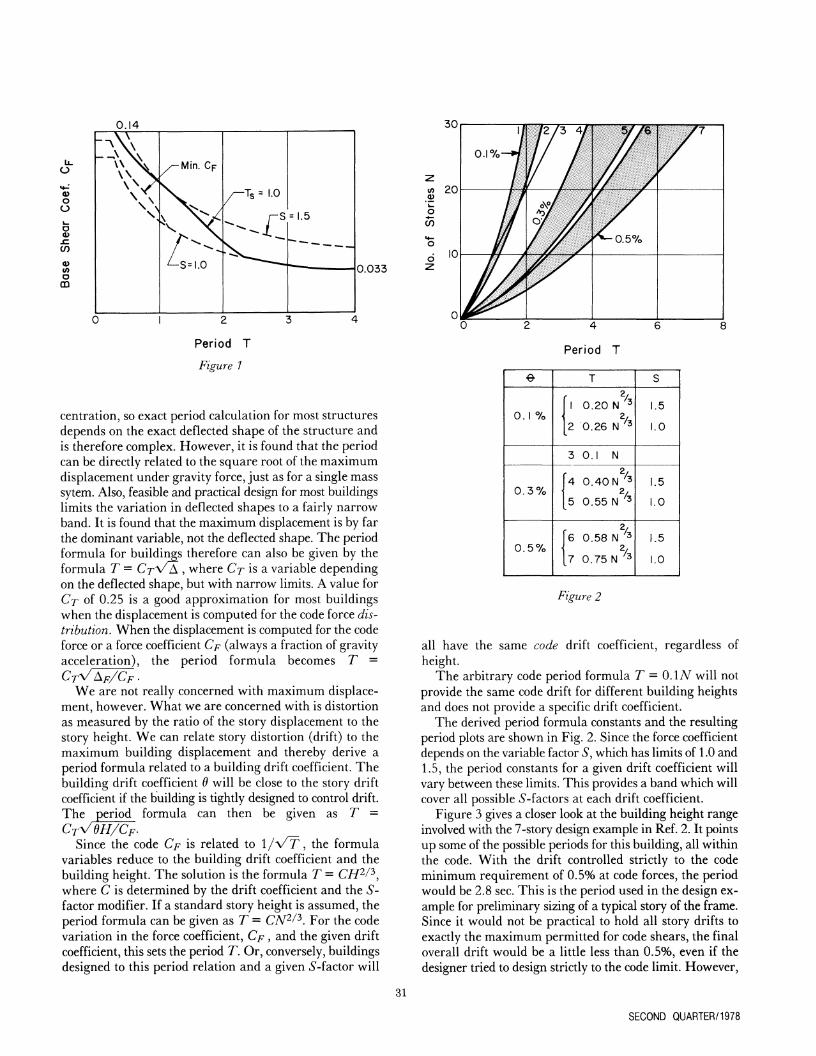
Since the code Cp is related to 1 / A / T , the formula variables reduce to the building drift coefficient and the building height. The solution is the formula T = CH^/^, where C is determined by the drift coefficient and the S-factor modifier. If a standard story height is assumed, the period formula can be given as 7" = CTV / . For the code variation in the force coefficient, Cp, and the given drift coefficient, this sets the period T. Or, conversely, buildings designed to this period relation and a given iS-factor will

30

en 20 0) v-O

5) O

6 10

1/

O.I7o-W

7 2 / 3 4 /

o\7 // ^/ // o7 //

S / / ^

-^O-S^/o

77 "

4

Period T

^

0.1 7o

0 . 3 %

0.57o

T

\ r ^/

1 0.20 N ^ 2/

2 0.26 N '^

3 0.1 N

r 2/ 14 0.40 N ^

[5 0.55 N ^

•

, 2 / 6 0.58 N 3

2/ 7 0.75 N 3

S

1.5

1.0

1.5

1.0

[.5

1.0

Figure 2

all have the same code drift coefficient, regardless of height.

The arbitrary code period formula T = O.IA^ will not provide the same code drift for different building heights and does not provide a specific drift coefficient.

The derived period formula constants and the resulting period plots are shown in Fig. 2. Since the force coefficient depends on the variable factor 5, which has limits of 1.0 and 1.5, the period constants for a given drift coefficient will vary between these limits. This provides a band which will cover all possible 5-factors at each drift coefficient.

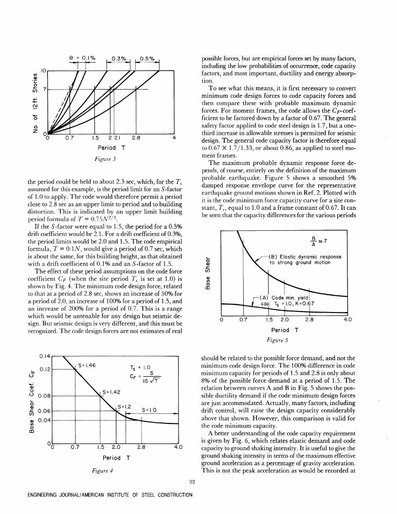
Figure 3 gives a closer look at the building height range involved with the 7-story design example in Ref. 2. It points up some of the possible periods for this building, all within the code. With the drift controlled strictly to the code minimum requirement of 0.5% at code forces, the period would be 2.8 sec. This is the period used in the design ex­ample for preliminary sizing of a typical story of the frame. Since it would not be practical to hold all story drifts to exactly the maximum permitted for code shears, the final overall drift would be a little less than 0.5%, even if the designer tried to design strictly to the code limit. However,

31

SECOND QUARTER/1978

9 =

i n , ' lU

<D k-

O W 7

^ «•-CVJ

— o

o ^ n

A //

/ / . / / / ///

f//A

/ /

0.17c > 0.3% , ,

•| i ^ 0 . 5 7 o ,

0.7 1.5 2 2.1 2.8

Period T

Figure 3

the period could be held to about 2.3 sec, which, for the T^ assumed for this example, is the period limit for an ^'-factor of 1.0 to apply. The code would therefore permit a period close to 2.8 sec as an upper limit to period and to building distortion. This is indicated by an upper limit building period formula of 7" = 0.7SN^^^.

If the ^-factor were equal to 1.5, the period for a 0.5% drift coefficient would be 2.1. For a drift coefficient of 0.3%, the period limits would be 2.0 and 1.5. The code empirical formula, T = OAN, would give a period of 0.7 sec, which is about the same, for this building height, as that obtained with a drift coefficient of 0.1% and an 5-factor of 1.5.

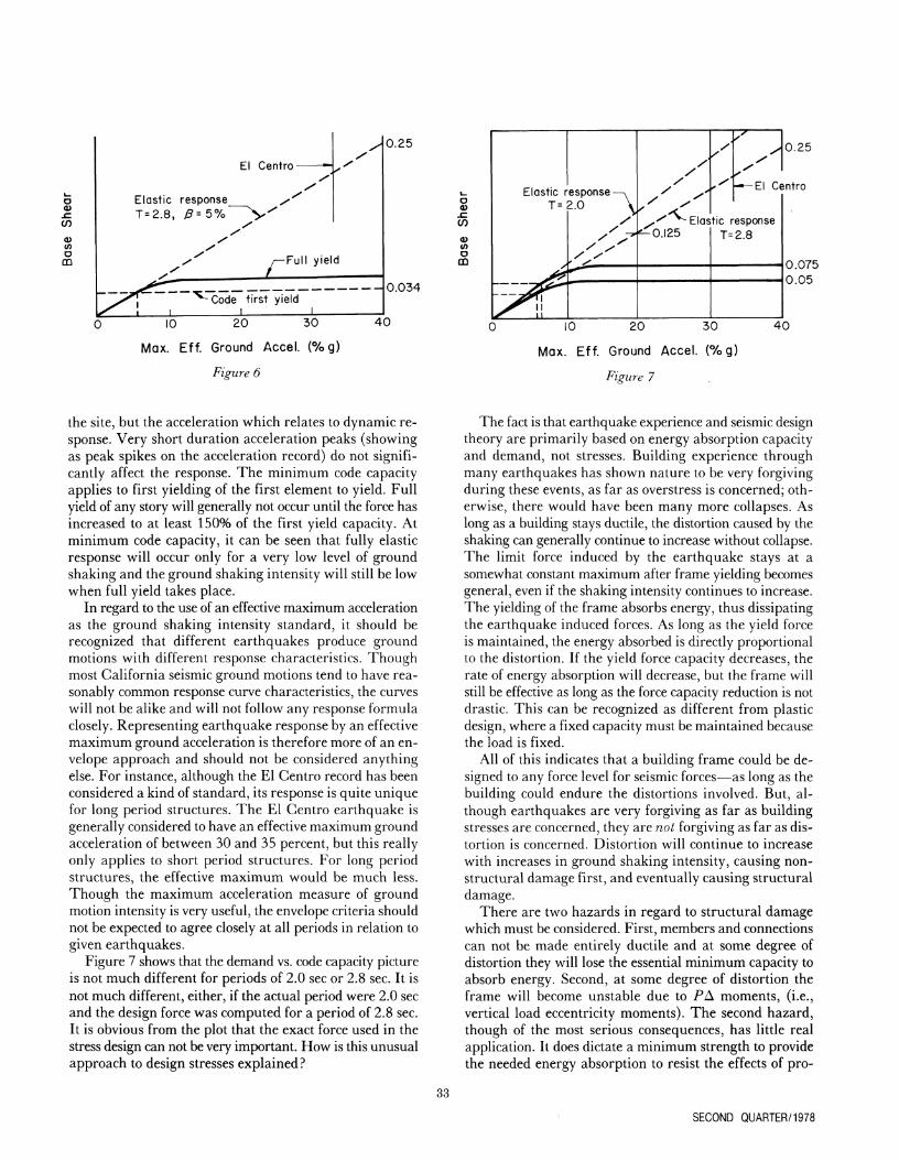
The effect of these period assumptions on the code force coefficient Cj7 (when the site period T^ is set at 1.0) is shown by Fig. 4. The minimum code design force, related to that at a period of 2.8 sec, shows an increase of 50% for a period of 2.0, an increase of 100% for a period of 1.5, and an increase of 200% for a period of 0.7. This is a range which would be untenable for any design but seismic de­sign. But seismic design is very different, and this must be recognized. The code design forces are not estimates of real

possible forces, but are empirical forces set by many factors, including the low probabilities of occurrence, code capacity factors, and most important, ductility and energy absorp­tion.

To see what this means, it is first necessary to convert minimum code design forces to code capacity forces and then compare these with probable maximum dynamic forces. For moment frames, the code allows the C/r-coef­ficient to be factored down by a factor of 0.67. The general safety factor applied to code steel design is 1.7, but a one-third increase in allowable stresses is permitted for seismic design. The general code capacity factor is therefore equal to 0.67 X 1.7/1.33, or about 0.86, as applied to steel mo­ment frames.

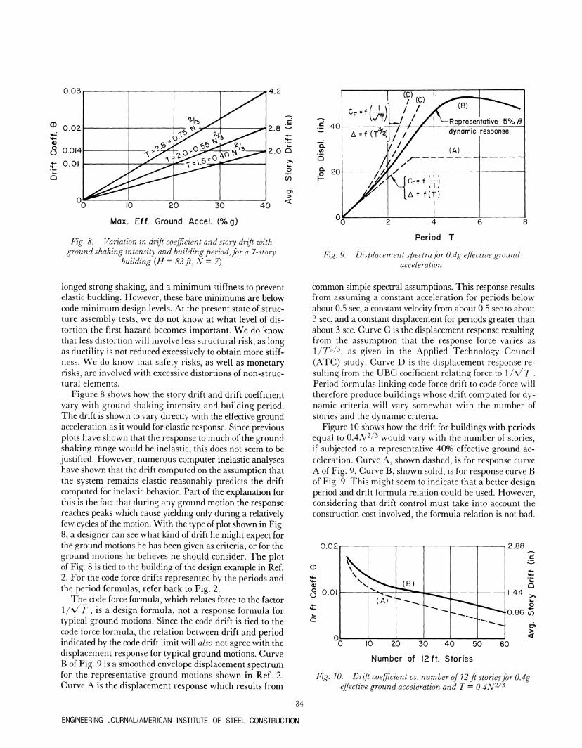
The maximum probable dynamic response force de­pends, of course, entirely on the definition of the maximum probable earthquake. Figure 5 shows a smoothed 5% damped response envelope curve for the representative earthquake ground motions shown in Ref. 2. Plotted with it is the code minimum force capacity curve for a site con­stant, T^, equal to 1.0 and a frame constant of 0.67. It can be seen that the capacity differences for the various periods

o 0)

(/)

o QD

« 7

-(B) Elastic dynamic response to strong ground motion

-(A) Code min. yield| cap. Ts = 1.0, K = 0.67

4.0

O

0) o o 1 _

o

if) to O

CD

0.14

0.12

0.08

0.06

0.04

I S = l . 4 6 To =

1 S= l .4 2

,S =

1.0 s

15 TT"

• s = io

0.7 1.5 2.0 2.8

Period T

Figure 4

4.0

should be related to the possible force demand, and not the minimum code design force. The 100% difference in code minimum capacity for periods of 1.5 and 2.8 is only about 8% of the possible force demand at a period of 1.5. The relation between curves A and B in Fig. 5 shows the pos­sible ductility demand if the code minimum design forces are just accommodated. Actually, many factors, including drift control, will raise the design capacity considerably above that shown. However, this comparison is valid for the code minimum capacity.

A better understanding of the code capacity requirement is given by Fig. 6, which relates elastic demand and code capacity to ground shaking intensity. It is useful to give the ground shaking intensity in terms of the maximum effective ground acceleration as a percentage of gravity acceleration. This is not the peak acceleration as would be recorded at

32

ENGINEERING JOURNAL/AMERICAN INSTITUTE OF STEEL CONSTRUCTION

o 0)

.c CO 0) to o CD

0.25

0.034

10 20 30

Max. Eff. Ground Accel. (%g)

Figure 6

o

if)

<n o

CD

0.25

K - E I Centro

H 0.075 0.05

10 20 30

Max. Eff. Ground Accel. (%g)

Figure 7

the site, but the acceleration which relates to dynamic re­sponse. Very short duration acceleration peaks (showing as peak spikes on the acceleration record) do not signifi­cantly affect the response. The minimum code capacity applies to first yielding of the first element to yield. Full yield of any story will generally not occur until the force has increased to at least 150% of the first yield capacity. At minimum code capacity, it can be seen that fully elastic response will occur only for a very low level of ground shaking and the ground shaking intensity will still be low when full yield takes place.

In regard to the use of an effective maximum acceleration as the ground shaking intensity standard, it should be recognized that different earthquakes produce ground motions with different response characteristics. Though most California seismic ground motions tend to have rea­sonably common response curve characteristics, the curves will not be alike and will not follow any response formula closely. Representing earthquake response by an effective maximum ground acceleration is therefore more of an en­velope approach and should not be considered anything else. For instance, although the El Centro record has been considered a kind of standard, its response is quite unique for long period structures. The El Centro earthquake is generally considered to have an effective maximum ground acceleration of between 30 and 35 percent, but this really only applies to short period structures. For long period structures, the effective maximum would be much less. Though the maximum acceleration measure of ground motion intensity is very useful, the envelope criteria should not be expected to agree closely at all periods in relation to given earthquakes.

Figure 7 shows that the demand vs. code capacity picture is not much different for periods of 2.0 sec or 2.8 sec. It is not much different, either, if the actual period were 2.0 sec and the design force was computed for a period of 2.8 sec. It is obvious from the plot that the exact force used in the stress design can not be very important. How is this unusual approach to design stresses explained?

The fact is that earthquake experience and seismic design theory are primarily based on energy absorption capacity and demand, not stresses. Building experience through many earthquakes has shown nature to be very forgiving during these events, as far as overstress is concerned; oth­erwise, there would have been many more collapses. As long as a building stays ductile, the distortion caused by the shaking can generally continue to increase without collapse. The limit force induced by the earthquake stays at a somewhat constant maximum after frame yielding becomes general, even if the shaking intensity continues to increase. The yielding of the frame absorbs energy, thus dissipating the earthquake induced forces. As long as the yield force is maintained, the energy absorbed is directly proportional to the distortion. If the yield force capacity decreases, the rate of energy absorption will decrease, but the frame will still be effective as long as the force capacity reduction is not drastic. This can be recognized as different from plastic design, where a fixed capacity must be maintained because the load is fixed.

All of this indicates that a building frame could be de­signed to any force level for seismic forces—as long as the building could endure the distortions involved. But, al­though earthquakes are very forgiving as far as building stresses are concerned, they are not forgiving as far as dis­tortion is concerned. Distortion will continue to increase with increases in ground shaking intensity, causing non­structural damage first, and eventually causing structural damage.

There are two hazards in regard to structural damage which must be considered. First, members and connections can not be made entirely ductile and at some degree of distortion they will lose the essential minimum capacity to absorb energy. Second, at some degree of distortion the frame will become unstable due to PA moments, (i.e., vertical load eccentricity moments). The second hazard, though of the most serious consequences, has little real application. It does dictate a minimum strength to provide the needed energy absorption to resist the effects of pro-

33

SECOND QUARTER/1978

0.03

10 20 30

Max. Eff. Ground Accel. (%g)

40

Fig. 8. Variation in drift coefficient and story drift with ground shaking intensity and building period, for a 7-story

building {H = 83 ft, N = 7)

.E 40

Q .

CL

,o

Period T

Fig. 9. Displacement spectra for 0.4g effective ground acceleration

longed strong shaking, and a minimum stiffness to prevent elastic buckling. However, these bare minimums are below^ code minimum design levels. At the present state of struc­ture assembly tests, we do not know at what level of dis­tortion the first hazard becomes important. We do know that less distortion will involve less structural risk, as long as ductility is not reduced excessively to obtain more stiff­ness. We do know that safety risks, as well as monetary risks, are involved with excessive distortions of non-struc­tural elements.

Figure 8 shows how the story drift and drift coefficient vary with ground shaking intensity and building period. The drift is shown to vary directly with the effective ground acceleration as it would for elastic response. Since previous plots have shown that the response to much of the ground shaking range would be inelastic, this does not seem to be justified. However, numerous computer inelastic analyses have shown that the drift computed on the assumption that the system remains elastic reasonably predicts the drift computed for inelastic behavior. Part of the explanation for this is the fact that during any ground motion the response reaches peaks which cause yielding only during a relatively few cycles of the motion. With the type of plot shown in Fig. 8, a designer can see what kind of drift he might expect for the ground motions he has been given as criteria, or for the ground motions he believes he should consider. The plot of Fig. 8 is tied to the building of the design example in Ref. 2. For the code force drifts represented by the periods and the period formulas, refer back to Fig. 2.

The code force formula, which relates force to the factor 1 / A / T , is a design formula, not a response formula for typical ground motions. Since the code drift is tied to the code force formula, the relation between drift and period indicated by the code drift limit will also not agree with the displacement response for typical ground motions. Curve B of Fig. 9 is a smoothed envelope displacement spectrum for the representative ground motions shown in Ref. 2. Curve A is the displacement response which results from

common simple spectral assumptions. This response results from assuming a constant acceleration for periods below about 0.5 sec, a constant velocity from about 0.5 sec to about 3 sec, and a constant displacement for periods greater than about 3 sec. Curve C is the displacement response resulting from the assumption that the response force varies as 1/7^/^, as given in the Applied Technology Council (ATC) study. Curve D is the displacement response re­sulting from the U B C coefficient relating force to l / V T . Period formulas linking code force drift to code force will therefore produce buildings whose drift computed for dy­namic criteria will vary somewhat with the number of stories and the dynamic criteria.

Figure 10 shows how the drift for buildings with periods equal to 0.47V^/^ would vary with the number of stories, if subjected to a representative 40% effective ground ac­celeration. Curve A, shown dashed, is for response curve A of Fig. 9. Curve B, shown solid, is for response curve B of Fig. 9. This might seem to indicate that a better design period and drift formula relation could be used. However, considering that drift control must take into account the construction cost involved, the formula relation is not bad.

0.02

O

5 0-0'

vV \ X

^^^*^ (AT"

^w^ " ^ -

^ • ^ -

" ^ - ~ "~-~-j

2.88

1.44 >

o 0.86 o)

> <

10 20 30 40 50

Number of 12ft. Stories

60

Fig. 10. Drift coefficient vs. number of 12-ft stories for 0.4g effective ground acceleration and T = O.dN'^^^

34

ENGINEERING JOURNAL/AMERICAN INSTITUTE OF STEEL CONSTRUCTION

100 "55 o a> if) - 1 - 8 0 o

o > N

{^

^

o c

c > O UJ

Xi o

CL

$5

c O

60

40

20

0

\ J

1

'2'll! ^ X ^

^ ^ ^

^/3

4.2

Q 2.0 >.

o CO

> <

10 20 30

Max. Eff. Ground Accel. (7og)

40

Fig. 11. Probability vs. drift for a 7-story building (H = 83 ft, N=7)

The cost of controlling drift increases as the buildings be­come shorter, because the response coefficient increases faster than the decrease in weight. Perhaps more significant is the fact that the weight of steel required to resist seismic forces becomes a larger percentage of the total steel weight as the buildings become shorter. The designer will generally find it much less strain to control probable earthquake drift for tall buildings than for short buildings. This is assuming that he controls chord drift in tall buildings by suitable framing systems, such as the tube system.

Figure 11 shows the key factors regarding distortion control: the drift and the probability of its occurrence, both related to ground motion intensity. For every site, a prob­ability curve can be drawn which relates the probability of occurrence to the ground motion intensity. Of course, this gets into the least known area of seismic design, but some probability estimate must be made by someone, consciously or intuitively. The probability curve in Fig. 11 shown is one estimate for an average site in California. All probability curves, regardless of their level, will have the general form of this curve. The probability curve shows about a 50% chance of getting 16%^ effective ground acceleration at least once in a 50-year period. This may be expected to cause about 1.6-in. story drift if a building with seven 12-ft stories were designed to the code drift limit period of 2.8 sec. T h e story drift if the period were 1.5 sec might be about 0.8 in. Bear in mind that the abscissa (%§• effective) is not the peak recorded ground acceleration, and the probability curve contains a considerable amount of judgment input. How­ever, it is on this type of analysis that the building seismic design should be based.

What has been the design practice drift control in Cal­ifornia?

Figure 12 shows building periods plotted vs. number of stories for the 16 Los Angeles area steel moment-frame buildings examined in Ref. 1. Most of the buildings were not designed by computer, but all of the buildings were later

60

(A

"»_ o 00 40

CJ

o .. 20

E 3

Los Angeles Area bidgs. + Offices 1 1 o Hospital o School

T=O.I N -y/^

^ +

0^0*^

/^ •¥ y

X T o y ^ ^ ^ T = 0 . 4 N

O

^^y

+

^'^^

^T = 0.75 N p

1 1

"^ 0.6%

Z

1.07o O

1.0%

l.57o >< o IE

0 1 2 3 4 5 6

Period T

Fig. 12. Building period vs. number of stories for 16 Los Angeles buildings

analyzed by computer. The code did not include a drift limit when these buildings were designed, so drift control for these buildings was strictly a matter of engineering judg­ment. Plotted for reference are the curves for three period formulas: the arbitrary code formula 7" = O.IA^, the formula T = 0.4A^2/3 (^^hich is derived for 0.3% drift at a code force coefficient Cp = O . I O / A / T ) , and the formula T = 0.75A^2/^ (which is derived for 0.5% drift at a code force coefficient Cp = 0.067/\/T). On the right margin of Fig. 12 is shown the maximum drift coefficient for the T = 0.47V2/3 curve, on the basis of a 40%^ effective ground ac­celeration. These numbers are taken from Fig. 10.

How good is the projection of elastic response data for inelastic response?

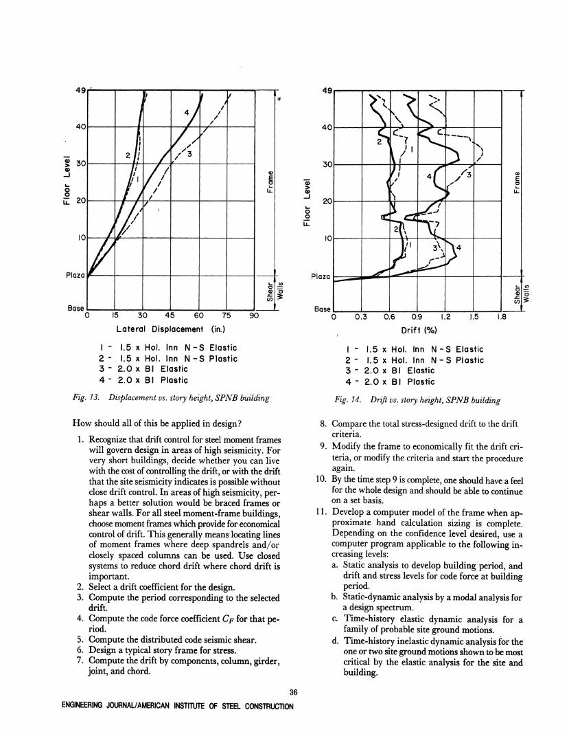
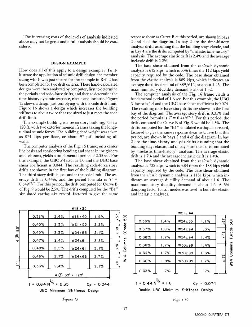
The Security Pacific National Bank (SPNB) building was analyzed by a time-history elastic program for seven ground motions indicated by seismologist consultants as representative of maximum credible ground motions for the site. The base shear indicated for two of these ground motions was about 50% greater than the computed frame capacity at beginning of full yield. The San Fernando earthquake Holiday Inn record, factored up by 50%, was one of these two, so it was used in an inelastic time-history computer program to check the inelastic response. Figures

13 and 14 show that this produced very little difference from a fully elastic analysis. In order to get a better check, the other record, the California Institute of Technology's Bl simulated earthquake record, was used in another in­elastic check. The elastic run was at 1.3 times the B l , but, to insure major inelastic action, the Bl record was factored by 2 for the inelastic run. There is more difference between elastic and inelastic response for this ground motion. However, this, as with other inelastic analyses, seems to indicate that assuming fully elastic response provides a reasonable response estimate, even when the response is in the inelastic range.

35

40

1 30 Q>

-J O o i l 20

10

Plaza

Base

11

2 / / II II

If

//

/ / / / ' / /

4/

/ /

1

/ / / / /

/ ' " • '

E o

o JC

'

€'

V)

1 0 15 30 45 60 75 90

Lateral Displacement (in.)

1 - 1.5 X Hoi. Inn N - S Elastic 2 - 1.5 X Hoi. Inn N - S Plastic 3 - 2 .0 X Bl Elastic 4 - 2.0 X Bl Plastic

Fig. 13. Displacement vs. story height, SPNB building

How should all of this be applied in design?

1. Recognize that drift control for steel moment frames will govern design in areas of high seismicity. For very short buildings, decide whether you can live with the cost of controlling the drift, or with the drift that the site seismicity indicates is possible without close drift control. In areas of high seismicity, per­haps a better solution would be braced frames or shear walls. For all steel moment-frame buildings, choose moment frames which provide for economical control of drift. This generally means locating lines of moment frames where deep spandrels and/or closely spaced columns can be used. Use closed systems to reduce chord drift where chord drift is important.

2. Select a drift coefficient for the design. 3. Compute the period corresponding to the selected

drift. 4. Compute the code force coefficient Cp for that pe­

riod. 5. Compute the distributed code seismic shear. 6. Design a typical story frame for stress. 7. Compute the drift by components, column, girder,

joint, and chord.

>

o o

Plaza

Base 0.6 0.9 1.2

Drift (7o)

1 - 1.5 X Hoi. Inn N - S 2 - 1.5 X Hoi. Inn N - S 3 - 2.0 X Bl Elastic 4 - 2.0 X Bl Plastic

Elastic Plastic

11

Fig. 14. Drift vs. story height, SPNB building

8. Compare the total stress-designed drift to the drift criteria.

9. Modify the frame to economically fit the drift cri­teria, or modify the criteria and start the procedure again.

10. By the time step 9 is complete, one should have a feel for the whole design and should be able to continue on a set basis. Develop a computer model of the frame when ap­proximate hand calculation sizing is complete. Depending on the confidence level desired, use a computer program applicable to the following in­creasing levels: a. Static analysis to develop building period, and

drift and stress levels for code force at building period.

b. Static-dynamic analysis by a modal analysis for a design spectrum.

c. Time-history elastic dynamic analysis for a family of probable site ground motions.

d. Time-history inelastic dynamic analysis for the one or two site ground motions shown to be most critical by the elastic analysis for the site and building.

36

ENGINEERING JOURNAL/AMERICAN INSTITUTE OF STEEL CONSTRUCTION

The increasing costs of the levels of analysis indicated above may not be great and a full analysis should be con­sidered.

DESIGN EXAMPLE

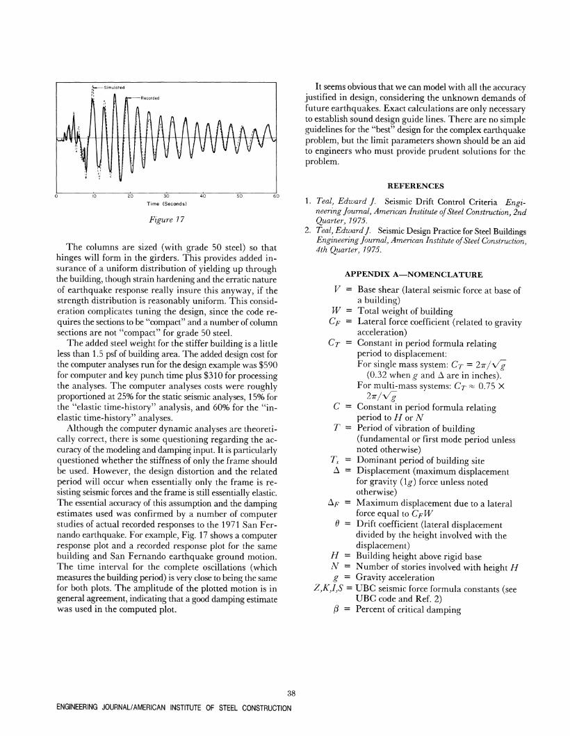
How does all of this apply to a design example? To il­lustrate the application of seismic drift design, the member sizing which was just started for the example in Ref. 2 has been completed for two drift criteria. These hand-calculated designs were then analyzed by computer, first to determine the periods and code-force drifts, and then to determine the time-history dynamic response, elastic and inelastic. Figure 15 shows a design just complying with the code drift limit. Figure 16 shows a design which increases the building stiffness to about twice that required to just meet the code drift limit.

The example building is a seven story building, 75 ft x 120 ft, with two exterior moment frames taking the longi­tudinal seismic forces. The building dead weight was taken as 874 kips per floor, or about 97 psf, including all walls.

The computer analysis of the Fig. 15 frame, on a center line basis and considering bending and shear in the girders and columns, yields a fundamental period of 2.35 sec. For this example, the UBC ^'-factor is 1.0 and the UBC base shear coefficient is 0.044. The resulting code-force story drifts are shown in the first bay of the building diagram. The third story drift is just under the code limit. The av­erage drift is 0.44%, and the period formula is T = 0.64A^^/^. For this period, the drift computed for Curve B of Fig. 9 would be 2.5%. The drifts computed for the "Bl" simulated earthquake record, factored to give the same

response shear as Curve B at this period, are shown in bays 2 and 4 of the diagram. In bay 2 are the time-history analysis drifts assuming that the building stays elastic, and in bay 4 are the drifts computed by "inelastic time-history" analysis. The average elastic drift is 2.4% and the average inelastic drift is 2.2%.

The base shear obtained from the inelastic dynamic analysis is 612 kips, which is 5.46 times the 112 kips yield capacity required by the code. The base shear obtained from the elastic analysis is 889 kips, which indicates an average ductility demand of 889/612, or about 1.45. The maximum story ductility demand is about 1.52.

The computer analysis of the Fig. 16 frame yields a fundamental period of 1.6 sec. For this example, the UBC ^S-factor is 1.4 and the UBC base shear coefficient is 0.074. The resulting code-force story drifts are shown in the first bay of the diagram. The average story drift is 0.35% and the period formula is 7" = 0.44A^2/3 YOT this period, the drift computed for Curve B of Fig. 9 would be 1.5%. The drifts computed for the "Bl" simulated earthquake record, factored to give the same response shear as Curve B at this period, are shown in bays 2 and 4 of the diagram. In bay 2 are the time-history analysis drifts assuming that the building stays elastic, and in bay 4 are the drifts computed by "inelastic time-history" analysis. The average elastic drift is 1.7% and the average inelastic drift is 1.4%.

The base shear obtained from the inelastic dynamic analysis is 722 kips, which is 3.84 times the 188 kips yield capacity required by the code. The base shear obtained from the elastic dynamic analysis is 1151 kips, which in­dicates an average ductility demand of about 1.6. The maximum story ductility demand is about 1.6. A 5% damping factor for all modes was used in both the elastic and inelastic analyses.

WIS x35 i

lO

(^ CD

V

0.387o

0.45%

0.45%

0.47%

0.49%

0.46%

0.36%

2.4%

2.37o

2.3%

2.4%

2.5%

2.7%

2.4%

4 @ 30

WI8x40

W2Ix55

W24x55

W24x6l

W24x6l

W24x68

' ^ 1 2 0 '

1.9%

2.2%

2.1%

2.27o

2. 1%

2.77o

2. l7o

^

roT ID xi

00 CD X

1 x\

i

X

1

W2I x44

T= 0 .64 N^^ = 2.35 Cp = 0.044

UBC Minimum Stiffness Design

o 0)

o i_

iD

C

E o o

0 . 3 6 %

0 . 3 7 %

0 .36%

0.367o

0 . 3 4 %

0.367o

[ 0 . 3 3 %

1.4%

1.8%

1 . 7 %

1.7%

1 .77o

l .87o

L 1 .77o

W24x55

W 2 4 x 9 4

W24x94

W30x99

W30x99

W30x99

1 . 1 %

1. 3%

1 . 4 %

1 . 4 %

1 . 3 %

1 . 7 %

1 .77o

00 x l

cvjj

— X

CD

X

T = 0 .44 N^^ = 1.6 Cp = 0.074

Double UBC Minimum Stiffness Design

o in

O

(/) c E o o

Figure 15 Figure 16

37

SECOND QUARTER/1978

Time (Seconds)

Figure 17

The columns are sized (with grade 50 steel) so that hinges will form in the girders. This provides added in­surance of a uniform distribution of yielding up through the building, though strain hardening and the erratic nature of earthquake response really insure this anyway, if the strength distribution is reasonably uniform. This consid­eration complicates tuning the design, since the code re­quires the sections to be "compact" and a number of column sections are not "compact" for grade 50 steel.

The added steel weight for the stiffer building is a little less than 1.5 psf of building area. The added design cost for the computer analyses run for the design example was $590 for computer and key punch time plus $310 for processing the analyses. The computer analyses costs were roughly proportioned at 25% for the static seismic analyses, 15% for the "elastic time-history" analysis, and 60% for the "in­elastic time-history" analyses.

Although the computer dynamic analyses are theoreti­cally correct, there is some questioning regarding the ac­curacy of the modeling and damping input. It is particularly questioned whether the stiffness of only the frame should be used. However, the design distortion and the related period will occur when essentially only the frame is re­sisting seismic forces and the frame is still essentially elastic. The essential accuracy of this assumption and the damping estimates used was confirmed by a number of computer studies of actual recorded responses to the 1971 San Fer­nando earthquake. For example. Fig. 17 shows a computer response plot and a recorded response plot for the same building and San Fernando earthquake ground motion. The time interval for the complete oscillations (which measures the building period) is very close to being the same for both plots. The amplitude of the plotted motion is in general agreement, indicating that a good damping estimate was used in the computed plot.

It seems obvious that we can model with all the accuracy justified in design, considering the unknown demands of future earthquakes. Exact calculations are only necessary to establish sound design guide lines. There are no simple guidelines for the "best" design for the complex earthquake problem, but the limit parameters shown should be an aid to engineers who must provide prudent solutions for the problem.

REFERENCES

1. Teal, Edward J. Seismic Drift Control Criteria Engi­neering Journal, American Institute of Steel Construction, 2nd Quarter, 1975.

2. Teal, Edward J. Seismic Design Practice for Steel Buildings Engineering Journal, American Institute of Steel Construction, 4th Quarter, 1975.

APPENDIX A—NOMENCLATURE

V =

w CF

Cr =

C =

T =

Base shear (lateral seismic force at base of a building) Total weight of building Lateral force coefficient (related to gravity acceleration) Constant in period formula relating period to displacement: For single mass system: CT — 27r/V^

(0.32 when g and A are in inches). For multi-mass systems: CT ^ 0.75 X

27r/V^ Constant in period formula relating period to H or N Period of vibration of building (fundamental or first mode period unless noted otherwise) Dominant period of building site Displacement (maximum displacement for gravity (1^) force unless noted otherwise) Maximum displacement due to a lateral force equal to Cj^W Drift coefficient (lateral displacement divided by the height involved with the displacement) Building height above rigid base Number of stories involved with height H Gravity acceleration

Z,K,I,S = UBC seismic force formula constants (see UBC code and Ref. 2)

13 = Percent of critical damping

A

A;. =

H N

g

38

ENGINEERING JOURNAL/AMERICAN INSTITUTE OF STEEL CONSTRUCTION