Seismic Damage Estimation in Buried Pipelines Due to ...cdn.intechweb.org/pdfs/30128.pdf · then, PGA can be directly obtained from seismic records without involving the integration

5

Seismic Damage Estimation in Buried Pipelines Due to Future Earthquakes – The Case of

the Mexico City Water System

Omar A. Pineda-Porras1 and Mario Ordaz2 1Energy and Infrastructure Analysis (D-4), Los Alamos National Laboratory, Los Alamos,

2Instituto de Ingeniería, Ciudad Universitaria, Universidad Nacional Autónoma de México (UNAM)

1USA 2Mexico

1. Introduction

Since the mid-70s, there have been advances in the development of models to better understand how earthquakes affect buried pipelines. These natural events can cause damage due to two phenomena: seismic wave propagation and permanent ground deformation. The combined effect of both phenomena in pipeline damage estimation is a subject still complex to address, especially if the objective is to estimate damage due to future earthquakes. In this chapter, the damage assessment methods only consider the impact of seismic wave propagation. The effects of permanent ground deformation phenomena, like ground subsidence, landslides, and ground rupture, are omitted. The exceptional damage caused by the 1985 Michoacan earthquake in Mexico City has encouraged researchers to develop sophisticated tools to estimate ground motion in the Valley of Mexico from Pacific coastal earthquakes, including the important site effects largely observed in the city. These tools have helped to better understand how earthquakes affect buildings and other structures like pipeline systems. The most remarkably case of pipeline damage caused by the 1985 seismic event is the extensive damage suffered by the Mexico City Water System (MCWS) that left almost 3.5 million people without water, and caused water service disruptions over a period of two months. The 1985 MCWS damage scenario has been extensively analyzed for developing models to better understand how seismic wave propagation affects buried pipelines; some of those models are employed in the future damage prediction methods described in this manuscript. Fragility functions are typically the tools most used to assess seismic damage in buried pipelines. These functions relate pipeline damage with seismic intensity. Pipeline damage is generally expressed as a linear pipe repair density. Seismic intensity is usually quantified through a seismic parameter. There are many seismic parameters used as arguments of fragility functions; the most important of these are described in Section 2. Section 3 describes the most important fragility functions proposed until now, including the two employed in the seismic damage estimation for the MCWS presented in Section 4. Finally, Section 5 contains a summary of the most important conclusions of this work.

www.intechopen.com

Earthquake-Resistant Structures – Design, Assessment and Rehabilitation

132

2. Seismic parameters related to damage in buried pipelines

An historical revision of all the seismic parameters employed to represent seismic intensity

in fragility functions is summarized in this section. The seismic parameters described in

detail are Mercalli modified intensity (MMI), peak ground acceleration (PGA), peak ground

velocity (PGV), maximum ground strain, and a recently proposed composite parameter

(Section 2.5). Other parameters used as fragility function arguments are not included here

because there is not enough evidence of their relationship with pipeline damage; among

them are permanent ground displacement, Arias intensity, spectral acceleration, and

spectral intensity.

2.1 Mercalli modified intensity Though it is a parameter of subjective nature, MMI was used as damage indicator for

pipelines in the 80s and 90s (Eguchi 1983 and 1991; Ballantyne et al. 1990; and, O’Rourke T.

et al. 1998). A likely reason for the development of MMI-based fragility relations in the past

was the extended use of that parameter to describe damage to aboveground structures.

Lately, the installation of seismic stations and the availability of seismic records have made

it easier to estimate parameters like PGA and PGV, which are better related to buried

pipeline damage.

2.2 Peak Ground Acceleration (PGA) PGA was largely employed as a damage indicator for pipelines during 25 years, from the

study of Katayama et al. (1975), to the PGA-based fragility function of Isoyama et al. (2000).

Though it has been largely demonstrated that PGV is related more closely to pipeline

damage than PGA, as it is further explained in the following paragraphs, there are several

reasons to explain why PGA, instead of PGV, was used to create some fragility functions

before 2000. Most seismic stations record time histories of acceleration instead of velocity;

then, PGA can be directly obtained from seismic records without involving the integration

process needed for computing PGV. Most attenuations laws provide estimates of PGA

(before 2000, PGV attenuation laws were limited); thus, for practical purposes, PGA was the

ideal parameter for analyzing pipeline damage, and therefore, creating pipeline fragility

relations.

2.3 Peak Ground Velocity (PGV) PGV is by far the most widely used seismic parameter for pipeline seismic fragility

functions. Generally, PGV shows good correlation with pipeline damage, although some

studies (Sections 2.4 and 2.5) have shown that, for pipeline located in soft soils, there are

some complications, mainly due to the assumptions related to PGV’s use as a damage

indicator.

PGV is better related to pipeline damage than PGA mainly due to two reasons: 1) PGV is

related to ground strain –the main cause of pipeline damage due to seismic wave

propagation (Section 2.3.2)–; and, 2) PGA is more related to inertia forces –forces that do not

affect buried structures like pipelines–. Many studies have empirically demonstrated that

PGV is better pipeline damage predictor than PGA (O’Rourke T. et al. 1998; Isoyama et al.

2000; and, Pineda 2002).

www.intechopen.com

Seismic Damage Estimation in Buried Pipelines Due to Future Earthquakes – The Case of the Mexico City Water System

133

PGV has been extensively used as damage indicator for pipelines considering two

assumptions: 1) PGV is directly related with maximum ground strain (g); and 2) transient ground strain is the main cause of pipeline damage due to seismic wave propagation. The

relationship between PGV and g can be analyzed in Equation 1 (Newmark 1967), where C is

seismic wave velocity. From Equation 1, PGV is directly related to g only if C is constant.

Since g is non-dimensional, PGV and C must be expressed with the same velocity units.

(1)

2.4 Maximum ground strain (g) Because transient ground strain is the assumed main cause of pipeline damage due to

seismic wave propagation, g is straightforwardly the optimum parameter for analyzing the

relationship between pipeline damage and seismic intensity. Rigorously, g can be estimated from displacement time histories D(t) (Equation 2). In Equation 2, x is a space variable, ε(t) is ground strain time history, and max represents the maximum of the expression between absolute value brackets | |.

(2)

There are three major problems for estimating g through Equation 2. First, g is generally

obtained through the double integration of acceleration time histories; this process causes loss

of information due to the involved mathematical operations. Procedures like correction of base

line, filtering and tapering could generate ambiguous results if the parameters used in those

operations are modified. Second, the derivation process of g with respect to a space variable

(x) implies that the seismic records used in the analysis need to be referenced to an absolute

time scale; this is a very significant limitation because only ground motion information from

seismic arrays using the same time reference, and preferably located in the place of interest

(e.g., the zone covered by a pipeline system), would be useful. The third and probably the

most important problem is the high cost involved in installing and operating seismic arrays

covering large extensions (e.g., area covered by a pipeline network).

In order to avoid the above-mentioned problems of Equation 2, Equation 1 has been used to

obtain conservative estimates of g. PGV can be easily obtained from seismic records or

other sources (e.g., attenuation laws); on the contrary, C is far from being easy to obtain,

which complicates the estimation of g. We include two examples to show the complexity of

estimating C for the purpose of estimating g with Equation 1.

In the first example, the g-based fragility relation proposed by O’Rourke and Deyoe (2004) was computed by assuming C values of 500 m/sec for Rayleigh waves (surface waves), and 3,000 m/sec for S-waves (body waves). Later, the study of Paolucci and Smerzini (2008) suggests that the apparent propagation velocity of S-waves is closer to 1,000 m/sec. O’Rourke M. (2009) employed the new suggested C value for S-waves and proposed a new version of the 2004 fragility relation. Changing C from 3,000 m/sec to 1,000 m/sec in

Equation 1 implies that g increases with a factor of three.

The second example deals with the estimation of g in soft soil zones. Singh et al. (1997) analyzed ground strains at the Roma micro-array in Mexico City for four earthquakes. They

www.intechopen.com


134

concluded that Equation 1 could be used to estimate g by using a phase velocity (Rayleigh waves) of 600 m/sec instead of the value of C at the natural period of lakebed sites (estimated as 1,500 m/sec). Singh et al. (1997) indicate that the discrepancy in the value of C could be due to local heterogeneities within the array. .

PGV is a more convenient parameter than g for analyzing pipeline damage due to seismic

wave propagation for three reasons. First, PGV is easier to estimate than g. Second, many studies have proved that PGV is well correlated with pipeline damage. Third, theoretically, there is a direct relationship between PGV and pipeline damage considering two assumptions already mentioned in this section. Notwithstanding these three points, there is evidence of a case in which PGV is not the best parameter for relating pipeline damage with seismic intensity: the particular case of Mexico City.

2.5 The novel composite parameter PGV²/PGA As it will be described in Section 3.4, Pineda and Ordaz (2007 and 2009) demonstrated that

PGV²/PGA is better correlated to pipeline damage than PGV alone for soft soils; a plausible

explanation for this is the strong relationship of PGV²/PGA to permanent ground

displacement (PGD), which is a ground motion parameter related to very-low frequency

contents. Though in the past O’Rourke (1998) demonstrated that PGV is better pipeline

damage predictor than PGD, studies that focused exclusively on the relationship between

pipeline damage and PGD (or PGV²/PGA) for soft soil sites have not been done yet. Finally,

two things must be noted: 1) Pineda and Ordaz (2007 and 2009) employed PGV²/PGA

instead of PGD due to the rigorous theoretical relationship between both parameters; the

availability of detailed PGA and PGV maps for the 1985 Michoacan event (see Pineda 2006

for details about those maps); and the lack of information on ground motion to produce

reliable PGD maps for the 1985 earthquake (Pineda 2006). Second, Pineda and Ordaz (2007

and 2009) define soft soils as those soils with natural periods equal to or higher than 1.0 sec.

3. Seismic fragility functions for buried pipelines

Buried pipeline seismic fragility functions relate pipeline damage rates with different levels

of seismic intensity. Damage rates are usually defined as the number of pipe repairs per unit

length of pipeline (e.g., number of repair per kilometer, rep/km). Seismic intensity can be

quantified through a diverse group of ground motion parameters computed from seismic

records (Section 2). Though there are many studies focused on computing analytical

pipeline fragilities (Hindy and Novak 1979; O’Rourke M. and El Hmadi 1988; and Mavridis

and Pitilakis 1996). This study only includes empirical pipeline fragility functions computed

from pipeline damage documented after earthquakes. For the sake of brevity, equations on

the fragility relations are not included here; but can be obtain from those studies in the

reference section of this chapter.

3.1 Early fragility functions for buried pipelines As noted previously, empirical correlation between buried pipeline damage and ground motion intensity parameters has been studied since the mid-70s. Katayama et al. (1975) employed pipeline damage scenarios from six earthquakes; four in Japan (Kanto, 9/01/1923; Fukui, 6/28/1948; Niigata, 6/16/1964; and, Tokachi-oki, 5/16/1968), one in Nicaragua (Managua, 12/23/1972), and one in the United States (San Fernando, 2/09/1971)

www.intechopen.com


135

to compute fragility functions for segmented cast iron (CI) and asbestos cement (AC) pipelines in terms of PGA. Katayama et al. (1975) included fragility functions for poor, average, and good soil conditions. Early in the 80s, Isoyama and Katayama (1982) employed the 1971 San Fernando earthquake damage scenario to compute a PGA-based fragility function. The same damage data and information on other three pipeline damage scenarios (Santa Rosa, 10/01/1969; Nicaragua, 12/23/1972; and Imperial Valley, 10/15/1979) was used by Eguchi (1983 and 1991) to compute a set of fragility functions in terms of MMI for the following pipeline types: welded steel gas welded joints (WSGWJ), AC, concrete (C), PVC, CI, welded steel caulked joints (WSCJ), welded steel arc-welded joints–Grades A & B steel (WSAWJ A&B), polyethylene (PE), ductile iron (DI), and welded steel arc-welded joints–Grade X steel–(WSAWJ X). Eguchi (1983 and 1991) concluded that AC and concrete pipes are more vulnerable than PVC pipes; and PVC pipes are more vulnerable than CI pipes and welded steel pipes with caulked joints. DI pipes experienced on average about 10 times fewer repairs per unit length than the worst performing pipes; and finally, the repair rate of X -grade steel pipes with arc-welded joints was approximately ten times smaller than that of DI pipes. In the late 80s, Barenberg (1988) proposed the first documented PGV-based fragility function for buried CI pipelines employing damage data from three U.S. earthquakes (Puget Sound, 4/29/1965; Santa Rosa, 10/01/1969; and, San Fernando, 2/09/1971). The fragility function of Barenberg (1988) suggests that a doubling of PGV will lead to an increase in the pipeline damage rate by a factor of about 4.5. Early in the 90s, Ballantyne et al. (1990) expanded the pipeline damage data of Barenberg

(1988) with damage information from other three U.S. earthquakes (Puget Sound,

4/29/1949; Coalinga, 5/02/1983; and Whittier Narrows, 10/01/1987) and proposed new

fragility functions by using MMI as a measure of seismic intensity.

Three PGA-based fragility functions were also published in the early 90s. The Technical

Council on Lifeline Earthquake Engineering (TCLEE) of the American Society of Civil

Engineers (ASCE) published a comprehensive study on seismic loss estimation for water

systems (ASCE-TCLEE 1991) in which PGA-based fragility relations were computed from a

reanalysis of the damage data of Katayama et al. (1975) and the 1983 Coalinga pipeline

damage scenario. Hamada (1991) proposed another PGA-based fragility function by

analyzing the damage scenarios of earthquakes from United States (San Fernando,

2/09/1971) and Japan (Miyagiken-oki, 6/12/1978; and Nihonkai-chubu, 5/26/1983).

O’Rourke T. et al. (1991) related pipeline damage with PGA employing damage scenarios

from seven earthquakes: six from U.S. (San Francisco, 4/18/1906; Puget Sound, 4/29/1965;

Santa Rosa, 10/01/1969; San Fernando, 2/09/1971; Imperial Valley, 10/15/1979; Coalinga,

5/02/1983; and Loma Prieta, 10/18/1989), and one from Japan (Miyagiken-oki, 6/12/1978).

3.2 Fragility functions in terms of PGV A notable change in the literature on seismic fragility functions for pipelines is observed from 1993, when PGV began to be the preferred seismic parameter for pipeline fragility relations, and PGA and MMI were no longer used for developing new fragility functions (with some exemptions described later in this section). O’Rourke and Ayala (1993) proposed a new pipeline fragility function in terms of PGV by using the damage data points of Barenberg (1988) and damage information from three earthquakes, one from the United States (Coalinga, 5/02/1983), and two from Mexico

www.intechopen.com


136

(Michoacan, 9/19/1985; and, Tlahuac, 4/25/1989). The damage data employed for computing the fragility function are related to pipelines made of AC, CI, concrete, and prestressed concrete cylinder pipes. The fragility relation of O’Rourke and Ayala (1993) was later incorporated into the U.S. Federal Emergency Management Agency’s loss assessment methodology HAZUS-MH (FEMA 1999). This fragility function can be used for damage prediction of brittle pipelines. For ductile pipelines, the fragility relation must be multiplied by a suggested factor of 0.3 (FEMA 1999). Eidinger et al. (1995) and Eidinger (1998) reanalyzed the pipeline damage data of O’Rourke

and Ayala (1993), along with information from the 1989 Loma Prieta pipeline damage

scenario, in order to propose a set of fragility functions in terms of PGV considering pipe

material, joint type, and soil corrosiveness. Edinger’s fragility functions estimated damage

for CI, welded steel (WS), AC, concrete, PVC, and DI pipes.

Hwang and Lin (1997) computed a pipeline fragility function in terms of PGA by

analyzing pipeline damage data obtained from six previous studies (Katayama et al. 1975;

Eguchi 1991; ASCE-TCLEE 1991; O’Rourke T. et al. 1991; Hamada 1991; and Kitaura and

Miyajima 1996).

O’Rourke T. et al. (1998) employed a GIS-based methodology to investigate factors affecting

the water supply service of the Los Angeles Department of Water and Power and the

Metropolitan Water District, after the 1994 Northridge earthquake. Analyses of the

relationship between damage rate and seismic intensity employed seven seismic

parameters: MMI, PGA, PGV, PGD, Arias Intensity, Spectral Acceleration, and Spectral

Intensity (SI). Pipeline fragility relations in terms of MMI, SI, PGA, and PGV, are also

included in the study. O’Rourke T. et al. (1998) concluded that PGV relates to the pipeline

damage better than any other parameter and proposed PGV-based fragilities for steel, CI,

DI, and AC pipelines. Later, O’Rourke T. and Jeon (1999) developed a fragility relationship

(for CI pipes) for scaled velocity, a parameter based on PGV but normalized for the effects of

pipe diameter.

Isoyama et al. (2000) computed fragility functions in terms of PGA and PGV by analyzing

the pipeline damage scenario left by the 1995 Hyogoken-nanbu earthquake. A multivariate

analysis computed empirical correction factors to account for pipe material, pipe diameter,

ground topography, and liquefaction, in the fragility relation.

The American Lifeline Alliance (ALA), a public-private partnership between the FEMA and

the ASCE, published a set of algorithms to compute the probability of damage from

earthquake effects to several components of water supply systems (ALA 2001). For buried

pipelines, the PGV-based fragility function published by the ALA was computed from a set

of 81 damage rate-PGV data points from 12 seismic damage scenarios. Similar to the

fragility functions of Eidinger et al. (1995) and Eidinger (1998), the ALA’s fragility relation

provides factor to account for pipe material, joint type, and soil corrosiveness.

Jeon and O’Rourke T. (2005) reanalyzed the pipeline damage data from a previous study

(O’Rourke T. et al. 1998). They compared the correlation between CI pipeline damage rates

from the 1994 Northridge earthquake and PGV computed in different ways (geometric

mean PGV, maximum PGV, and maximum vector magnitude of PGV). Their results show

that maximum PGV, computed as the peak recorded value, is better correlated with pipeline

damage. Jeon and O’Rourke T. (2005) also provide fragility functions for WSJ Steel, CI, DI,

and AC, pipelines.

www.intechopen.com


137

3.3 Fragility functions in terms of maximum ground strain O’Rourke M. and Deyoe (2004) analyzed the differences of the fragility relations

published by O’Rourke M. and Ayala (1993) and O’Rourke T. and Jeon (1999). The

analysis identified some reasons for the differences, including the wave type that

dominated each seismic scenario, the presence of corrosion in some pipes, and the low

statistical reliability of some data points. By removing doubtful data points and

classifying the remaining data points according to the presumably dominating wave type,

O’Rourke M. and Deyoe computed PGV-based pipeline fragility functions for surface

waves (Rayleigh) by assuming phase velocity of 500 m/sec, and body waves (S-waves) by

assuming apparent velocity of 3,000 m/sec. They also proposed a fragility function in

terms of g. The new g-based fragility function also considers the effect of permanent

ground deformation because O’Rourke and Deyoe (2004) included repair rate-g data

points from the 1994 Northridge earthquake (Sano et al. 1999) and from Japan (Hamada

and Akioka 1997). A recent modification to the g-based fragility relation (O’Rourke M.

2009) uses an apparent velocity of 1000 m/sec for S-waves; they base that assumption on a

study by Paolucci and Smerzini (2008).

3.4 Seismic fragility functions based on the 1985 MCWS damage scenario In the literature, there are two observed tendencies for developing fragility functions: the

use of damage scenarios for several pipelines systems and earthquakes; and the use of

damage scenarios for only a specific pipeline system and earthquake. On the one hand,

while the first tendency provides general pipeline fragilities, characterized by its wide

applicability due to the typical mixture of pipeline types and other factors (ALA, 2001), it is

also usually related to high uncertainty levels. On the other hand, using information about a

specific pipeline system and well-studied damage scenarios, the uncertainty could be

controlled because the number of unknown variables related to pipeline damage (e.g.,

variables related to earthquake environment, soil properties, and pipeline conditions), for

that particular study case, is lower than if several systems and events are included in the

analysis. In order to reduce the uncertainty in the damage estimation for the MCWS, in this

study only two fragility functions (Pineda and Ordaz, 2003 and 2007) are used to estimate

the damage in the pipeline system.

Pineda and Ordaz (2003) proposed a fragility formulation for buried pipelines employing

the 1985 damage scenario published by Ayala and O’Rourke M. (1989), and the detailed

maps for Mexico City proposed by Pineda and Ordaz (2004). In order to analyze the

variability of the relationship between damage rates (rep/km) and PGV for several ranges

of seismic intensity, nine scenarios were used to generate a PGV-based fragility function. In

this study, the functional form chosen for the fragility relation is the cumulative normal

function because it better fit the cloud of damage rate-PGV data points when compared with

the resulting fit employing other function types (linear, power, etc.). This fragility function is

employed in the damage assessment of Section 4.2.

In a subsequent study, Pineda and Ordaz (2007) proposed PGV²/PGA as a new seismic

parameter for buried pipelines. From a theoretical development, they found that pr, defined

by Equation 3, interrelate the peak ground response parameters PGA, PGV, and PGD. pr

has three relevant characteristics: it is non-dimensional; it is always greater than or equal to

1.0; and it can be a measure of spectra bandwidth.

www.intechopen.com


138

(3)

By isolating PGD in Equation 3, it is found that PGD and PGV²/PGA have a direct

relationship through pr (Equation 4). Based on the assumption that ground strain, the main cause for the pipeline damage, is related to PGD; pipeline damage is then also related to

PGV²/PGA and pr. Because pr varies in a delimited range for the places where the MCWS is located in Mexico City, it was implicitly included in the fragility formulation. This PGV²/PGA-based fragility function is used in the damage assessment discussed in Section 4.3.

(4)

Recently, Pineda and Ordaz (2009) computed fragility relations for 48-inch segmented pipelines considering the effects of ground subsidence, a phenomenon largely observed in the Valley of Mexico. They analyzed the relationship between pipeline damage and seismic intensity (measured in terms of PGV²/PGA) for two levels of differential ground subsidence (DGS). The proposed fragility functions fall above and below a previous fragility relation for 48-inch pipelines that does not explicitly consider the effects of DGS in the damage (Pineda 2006).

4. Seismic damage estimation in the MCWS due to future earthquakes

The main objective of this section is to describe a new approach for estimating pipeline damage at the MCWS due to future earthquakes nucleated at the subduction zones of the Pacific Mexican coast. This new study is based on a fragility function in terms of PGV²/PGA (a seismic parameter described in Section 2.5) that has shown better correlation with buried pipeline damage (Pineda and Ordaz, 2007) than PGV alone. Pineda and Ordaz (2003) previously employed this parameter to predict future damage at the MCWS.

4.1 Description of the MCWS and its 1985 damage scenario The MCWS pipeline network is formed by more than 600 km of pipes, with diameters ranging from 20- to 72-inches, and made of several pipe materials: asbestos-cement, concrete, cast iron, and steel. This pipeline system is particularly vulnerable to earthquakes because it is mainly located in the lake zone of the Valley of Mexico where deep clay deposits cause great dynamic amplification of seismic waves. The MCWS was severely affected by the 1985 earthquake, causing extensive damage that

left around 40% of the 8.5 million people living in the Federal District without water service.

A comprehensive report on the damage was published by Ayala and O’Rourke M. (1989).

They observed that two-thirds of the damage was located at pipe joints; and that the

observed failure types include lateral crushing of pipes, and crushing and unplugging of

joints. The authors state that the main apparent cause for the extensive damage in the

pipeline network was the propagation of surface waves (Rayleigh waves). These greatly

amplified waves caused that most of the damage were localized in sites with natural period

higher than 2 s, and with clay deposits between 30-m and 70-m deep. The authors also

indicate that the second most important factor that likely influenced the great damage in the

pipeline system was the largely observed ground settlement typical of the lake zone, a

phenomenon that could have reduced the pipeline capacity to withstand wave propagation.

www.intechopen.com


139

4.2 General aspects of the estimation of future damage in the MCWS The MCWS 1985 damage scenario has been used to compute fragility functions to better understand the relationship between pipeline damage and seismic intensity (Section 3.4). Two of those fragility functions, the one in terms of PGV (Pineda and Ordaz, 2003), and another in terms of PGV²/PGA (Pineda and Ordaz, 2007) are used in the future damage estimation described in Sections 4.3 and 4.4, respectively. In general, the procedure to estimate the expected number of pipe repairs for a set of earthquake scenarios is the same, independently of the seismic parameter of interest (PGV or PGV²/PGA). The main steps are 1) A set of postulated earthquake scenarios is calculated with the Program Z (Ordaz et al. 1996) for magnitudes (m) between 6.6 and 8.4, and for focal distances (R) between 250 and 450 km. 2) The MCWS network is divided in segments of 100 m or shorter, and the seismic parameter value (PGV or PGV²/PGA) is calculated at each segment mid-point for each earthquake scenario. 3) The expected number of pipe repairs for each earthquake scenario is then computed by adding all the damage rate-length products for the whole pipeline network. The summary of these calculations is shown in Sections 4.3 and 4.4.

4.3 Future damage estimation using PGV Based on the 1985 MCWS pipeline damage scenario, Pineda and Ordaz (2003) proposed a fragility function to estimate damage to buried pipelines. In Figure 1 the fragility function is showed along with the data points employed in its calculation. The 1985 damage scenario was divided in zones depending on the PGV values; a total of nine different PGV intervals (I1 to I9 in Figure 1) were used to generate the data points for the relationship damage rate-PGV. More details about the calculation of this fragility curve are found at the 2003 paper. In

Equation 5, RR is the expected number of pipe repairs per kilometer of pipeline,

represents the cumulative normal function defined by Equation 6, where and are parameters related to the mean and standard deviation of the damage rate-PGV relationship. In Equations 5 and 6, PGV is in cm/sec.

(5)

(6)

A total of 75 earthquakes scenarios were employed to estimate the MCWS damage due to future seismic events nucleated at the subduction zones of the Pacific Mexican coast. These scenarios represent events with magnitudes between 6.6 and 8.4, and focal distances between 250 and 450 km. The number of pipe repairs for each scenario was rounded to the nearest integer (Table 1). These results can also be observed in Figure 2. It is observed that for magnitudes higher than 7.6, there is an exponential tendency in the variation of the number of repairs (NR), and magnitude. In fact, after fitting a double exponential function in terms of m and R, an equation to simplify the estimation of NR was obtained (Equation 7). NR, then, can be estimated with Equation 7 (where e is the exponential parameter) for earthquake scenarios with magnitudes equal or higher than 7.6, and focal distances between

www.intechopen.com


140

250 km and 450 km. The fitting of Equation 7 is a good representation of the damage estimates from Table 1 because the R-square parameter was 0.996. The results for magnitudes lower than 7.6 did not have any clear tendency on the m and R domains, so it was no possible to find a similar function to the one shown in Equation 7.

(7)

Equation 7 shows how NR is related to m and R; however, for a better damage prediction, the figures from Table 1 must have preference over calculations with the equation due to the added error caused by the fitting.

Fig. 1. Fragility Function for the MCWS in terms of PGV (Pineda and Ordaz, 2003). Di is damage rate in number of pipe repairs per kilometer of pipeline (it is also called RR in this manuscript)

www.intechopen.com


141

FOCAL DISTANCE

MAGNITUDE R = 250 km R = 300 km R = 350 km R = 400 km R = 450 km

6.6 1 0 0 0 0

6.7 4 1 0 0 0

6.8 10 3 1 0 0

6.9 18 7 2 1 0

7.0 27 15 7 2 1

7.1 38 24 13 7 3

7.2 47 35 23 14 7

7.3 54 42 33 23 14

7.4 59 50 40 33 23

7.5 66 57 47 39 32

7.6 76 63 54 45 38

7.8 102 89 70 60 51

8.0 141 115 98 87 68

8.2 208 165 134 113 99

8.4 289 240 198 163 136

Table 1. Expected number of pipe repairs in the MCWS due to postulated earthquake scenarios (PGV-based model; Pineda and Ordaz, 2003)

Fig. 2. Seismic damage prediction model for the MCWS based on a PGV-based fragility function (Pineda and Ordaz, 2003)

www.intechopen.com


142

4.4 Future damage estimation using the composite parameter PGV²/PGA The PGV²/PGA-based fragility function proposed by Pineda and Ordaz (2007) for the MCWS (Figure 3) has three parts where the damage rate can be— zero, constant, or linearly dependent of PGV²/PGA (Equation 8). The no-damage zone is defined for seismic intensity levels not associated to pipeline damage in the 1985 damage scenario. A likely explanation of the constant-damage zone is the presumably about-to-fail precondition of some pipe segments previously to the 1985 event. The PGV²/PGA map employed by Pineda and Ordaz (2007) to generate the fragility function is shown in Figure 3.

(8)

In Figure 4, the PGV²/PGA-based fragility function is showed along with the data points employed in its calculation. In a similar way to the employed to calculate the PGV-based fragility function (Section 4.3), the 1985 damage scenario was divided in zones depending on the PGV²/PGA values; a total of nine different PGV²/PGA intervals (I1 to I9 in Figure 3) were used to generate the data points for the relationship damage rate- PGV²/PGA. The 2007 paper contains more details about the calculation of this fragility curve.

Fig. 3. Mexico City water system, PGV²/PGA map, and damage sites after the 1985 Michoacan earthquake

www.intechopen.com


143

Fig. 4. Fragility Function for the MCWS in terms of PGV²/PGA (Pineda and Ordaz, 2007). Di is damage rate (rep/km); it is also called RR through this manuscript

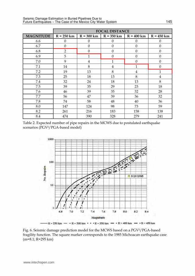
The damage estimation for the MCWS employing the fragility function in terms of PGV²/PGA was done with 80 earthquake scenarios calculated with the Program Z (Ordaz et al. 1996) for seismic events nucleated at the Mexican Pacific subduction zones with magnitudes between 6.6 and 8.4, and focal distances between 250 and 450 km, as it was done with the model described in Section 4.3. Figure 5 shows an example of postulated seismic scenario for a magnitude of 8.4 and focal distance of 250 km. This event is much stronger than the 1985 Michoacan event (m=8.1; R=295 km) because it has a larger magnitude and a shorter focal distance. The expected number of pipe repairs for the 80 earthquake scenarios are shown in Table 2 and plotted in Figure 6. In this prediction model, an exponential relationship between the number of pipe repairs and magnitude is observed for magnitudes higher than 7.8 for all focal distances; this relationship can be represented by the exponential function shown in Equation 9, where a and b are fitting parameters that vary depending on the focal distance values (Table 3). The fit of Equation 9 for all five focal distances is good because the R-square parameters have values close to one. Figure 7 shows the fitted curves with Equation 9 using the parameters from Table 3. These curves can be compared with the original data points from Table 2. Because there is no a clear tendency in the variation of NR with respect to m and R for magnitudes lower than 7.8, a fitted curve could not be found.

(9)

www.intechopen.com


144

Fig. 5. Earthquake scenario map for a postulated event (m=8.4; R=250km) and the MCWS

4.5 Comparison of results between the PGV and PGV²/PGA models A comparison between both prediction models reveals that the PGV²/PGA-based model (Section 4.4) predicts a lower number of pipe repairs than the PGV-based model (Section 4.3), for magnitudes around 8.0 and lower; and for higher magnitudes, the PGV²/PGV-based model predicts a higher number of pipe repairs (Figure 8). These results mean that the 2003 model overestimates the damage in the MCWS for earthquakes with magnitudes up to 8.0, and underestimates damage figures for stronger earthquakes. This conclusion is based on the fact that the proposed model uses a parameter better related to buried pipeline damage. One important advantage of the PGV²/PGA model is the linear relationship between RR and PGV²/PGA in the fragility function. This simple functional form makes it easier to assess the damage for very strong earthquakes (events stronger than the 1985 quake). On the contrary, the PGV model could be unreliable for earthquakes stronger than the 1985 quake because the PGV-based fragility function assumes a linear relationship RR-PGV for PGV values higher than 95 cm/sec, something that could not be demonstrated in the 2003 study.

www.intechopen.com


145

FOCAL DISTANCE

MAGNITUDE R = 250 km R = 300 km R = 350 km R = 400 km R = 450 km

6.6 0 0 0 0 0

6.7 0 0 0 0 0

6.8 2 0 0 0 0

6.9 5 1 0 0 0

7.0 9 4 1 0 0

7.1 14 8 4 1 0

7.2 19 13 8 4 1

7.3 25 18 13 8 4

7.4 32 24 18 13 8

7.5 39 35 29 23 18

7.6 46 39 35 32 28

7.7 56 47 39 36 32

7.8 74 58 48 40 36

8.0 147 124 98 73 59

8.2 261 216 183 158 138

8.4 474 390 328 279 241

Table 2. Expected number of pipe repairs in the MCWS due to postulated earthquake scenarios (PGV²/PGA-based model)

Fig. 6. Seismic damage prediction model for the MCWS based on a PGV²/PGA-based fragility function. The square marker corresponds to the 1985 Michoacan earthquake case (m=8.1; R=295 km)

www.intechopen.com


146

Fig. 7. Fitted curves for Equation 9

FOCAL DISTANCE

R = 250 km R = 300 km R = 350 km R = 400 km R = 450 km

a 2.972E-09 1.448E-09 8.453E-10 2.916E-10 2.927E-10

b 3.073 3.1369 3.18 3.287 3.268

R² 0.998 0.995 0.998 0.997 0.99

Table 3. Parameters a and b for Equation 9, and R-square parameters

www.intechopen.com


147

Fig. 8. Comparison of results between the PGV and PGV²/PGA models

5. Conclusions

One important challenge in the field of earthquake engineering for pipelines is the damage estimation due to future events. In this chapter, the reader will find a comprehensive state-of-the-art revision of the seismic parameters that have been employed as damage indicators for pipelines, and the most important seismic fragility functions proposed until now. In order to show a case of damage estimation due to future earthquake, we describe two prediction models for the Mexico City Water System (MCWS). The results of this research reveal that a previous damage estimation study for the MCWS, based on a PGV fragility function, overestimated the expected number of pipe repairs caused by earthquakes with magnitudes around 8.0 to 8.1 and lower, and underestimated the damage for stronger earthquakes. This new study employs a recently proposed fragility

www.intechopen.com


148

function for the MCWS in terms of PGV²/PGA: A composite parameter in terms of PGA, and PGV. Because a previous study (Pineda and Ordaz, 2007) demonstrates that PGV²/PGA is better related to pipeline damage in Mexico City than PGV alone, the results of the future damage estimation for the MCWS showen here are believed to be more reliable than those obtained with the PGV-based fragility function (Pineda and Ordaz, 2003).

6. Acknowledgements

This research has been partially funded by the Energy and Infrastructure Analysis (D-4) group at Los Alamos National Laboratory and the Institute of Engineering of the National Autonomous University of Mexico (UNAM).

7. References

American Lifelines Alliance, ALA (2001). Seismic Fragility Formulations for Water Systems, American Society of Civil Engineers (ASCE) and Federal Emergency Management Agency (FEMA). www.americanlifelinesalliance.org

ASCE-TCLEE (1991). Seismic Loss Estimation for a Hypothetical Water System. Technical Council on Lifeline Earthquake Engineering (TCLEE) of the American Society of Civil Engineers (ASCE), Monograph No.2, C.E. Taylor (eds).

Ayala, G. & O’Rourke, M. (1989). Effects of the 1985 Michoacan Earthquake on Water Systems and other Buried Lifelines in Mexico, Multidisciplinary Center for Earthquake Engineering Research, Technical Report NCEER-89-0009, New York.

Ballantyne, D. B.; Berg, E.; Kennedy, J.; Reneau, R. & Wu, D. (1990). Earthquake Loss Estimation Modeling for the Seattle Water System, Report to U.S. Geological Survey under Grant 14-08-0001-G1526, Technical Report, Kennedy/Jenks/Chilton, Federal Way, WA.

Barenberg, M.E. (1988). Correlation of Pipeline Damage with Ground Motions. Journal of Geotechnical Engineering, ASCE, June, 114 (6), 706-711.

Eidinger, J. (1998). Water Distribution System – The Loma Prieta, Californa, Earthquake of October 17, 1989 - Lifelines, USGS, Professional Paper 1552-A, Anshel J. Schiff (ed.), U.S. Government Printing Office, Washington, A63-A78.

Eidinger, J.; Maison, B.; Lee, D. & Lau, B. (1995). East Bay Municipal District Water Distribution Damage in 1989 Loma Prieta Earthquake. Proceedings of the Fourth U.S. Conference on Lifeline Earthquake Engineering, ASCE-TCLEE, Monograph No. 6, 240-247.

Eguchi, R. T. (1983). Seismic Vulnerability Models for Underground Pipes. Proceedings of Earthquake Behavior and Safety of Oil and Gas Storage Facilities, Buried Pipelines and Equipment, ASME, PVP-77, New York, June, 368-373.

Eguchi, R. T. (1991). Seismic Hazard Input for Lifeline Systems. Structural Safety, 10, 193-198. FEMA (1999). Earthquake Loss Estimation Methodology HAZUS-MH – Technical Manual. FEMA,

Washington DC, http://www.fema.gov/hazus. Hamada, M. (1991). Estimation of Earthquake Damage to Lifeline Systems in Japan.

Proceedings of the Third Japan-U.S. Workshop on Earthquake Resistant Design of Lifeline Facilities and Countermeasures for Soil Liquefaction, San Francisco, CA, December 17-19, 1990; Technical Report NCEER-91-0001, NCEER, State University of New York at Buffalo, Buffalo, NY, 5-22.

www.intechopen.com


149

Hamada, M. & Akioka, Y. (1997). Liquefaction Induced Ground Strain and Damage to Buried Pipes. Proceedings of Japan Society of Civil Engineers Earthquake Engineering Symposium, Vol. 1, pp. 1353–1356 (in Japanese).

Hindy, A. & Novak, M. (1979). Earthquake Response of Underground Pipelines. Earthquake Engineering and Structural Dynamics, 106, 451–476.

Hwang, H. & Lin, H. (1997). GIS-based Evaluation of Seismic Performance of Water Delivery Systems. Technical Report, CERI, University of Memphis, Memphis, TN.

Isoyama, R.; Ishida, E.; Yune, K. & Shirozu, T. (2000). Seismic Damage Estimation Procedure for Water Supply Pipelines. Proceedings of the Twelfth World Conference on Earthquake Engineering, CD-ROM Paper No. 1762, 8pp.

Isoyama, R. & Katayama, T. (1982). Reliability Evaluation of Water Supply Systems during Earthquakes. Report of the Institute of Industrial Science, University of Tokyo, 30 (1) (Serial No. 194).

Jeon, S. S. & O’Rourke, T. D. (2005). Northridge Earthquake Effects on Pipelines and Residential Buildings. Bulletin of the Seismological Society of America, 95 (1), 294-318.

Katayama, T.; Kubo, K. & Sato, N. (1975). Earthquake Damage to Water and Gas Distribution Systems. Proceedings of the U.S. National Conference on Earthquake Engineering, EERI, Oakland, CA, 396-405.

Kitaura, M. & Miyajima, M. (1996). Damage to Water Supply Pipelines. Special Issue of Soils and Foundations. Japanese Geotechnical Society, Japan, January, 325-333.

Mavridis, G. & Pitilakis, K. (1996). Axial and Transverse Seismic Analysis of Buried Pipelines. Proceedings of the Eleventh World Conference on Earthquake Engineering, Acapulco, Mexico, 81-88.

Newmark, N. M. (1967). Problems in Wave Propagation in Soil and Rocks. Proceedings of the International Symposium on Wave Propagation and Dynamic Properties of Earth Materials, University of New Mexico Press.

Ordaz, M.; Perez Rocha, L.E.; Reinoso, E.; Montoya, C. & Arboleda, J. (1996-2002) Program Z, Instituto de Ingeniería, National Autonomous University of Mexico (UNAM).

O’Rourke, M. J. (2009). Analytical Fragility Relation for Buried Segmented Pipe. Proceedings of the TCLEE 2009: Lifeline Earthquake Engineering in a Multihazard Environment. Oakland, CA, 771-780.

O'Rourke, M. J. & Ayala, G. (1993). Pipeline Damage due to Wave Propagation. Journal of Geotechnical Engineering, ASCE, 119 (9), 1490-1498.

O’Rourke, M. J. & Deyoe, E. (2004). Seismic Damage to Segmented Buried Pipe. Earthquake Spectra, (20) 4, 1167–1183.

O’Rourke, M. J. & El Hmadi, K. (1988). Analysis of Continuous Buried Pipelines for Seismic Wave Effects. Earthquake Engineering and Structural Dynamics, 16, 917-929.

O’Rourke, T. D. & Jeon, S. S. (1999). Factors Affecting the Earthquake Damage of Water Distribution Systems. Proceedings of the Fifth U.S. Conference on Lifeline Earthquake Engineering, Seattle, WA, ASCE, Reston, VA, 379-388.

O’Rourke, T. D.; Stewart, H. E.; Gowdy, T. E. & Pease, J. W. (1991). Lifeline and Geotechnical Aspects of the 1989 Loma Prieta Earthquake. Proceedings of the Second International Conference on Recent Advances in Geotechnical Earthquake Engineering and Soil Dynamics, St. Louis, MO, 1601-1612.

www.intechopen.com


150

O'Rourke, T. D.; Toprak, S. & Sano, Y. (1998). Factors Affecting Water Supply Damage Caused by the Northridge Earthquake. Proceedings of the Sixth U.S. National Conference on Earthquake Engineering.

Paolucci, R. & Smerzini, C. (2008). Earthquake-induced Transient Ground Strains from Dense Seismic Networks. Earthquake Spectra, 24 (2), 453-470.

Pineda, O. (2002). Estimación de Daño Sísmico en la Red Primaria de Distribución de Agua Potable del Distrito Federal. Master of Engineering Thesis, Institute of Engineering, National Autonomous University of Mexico (UNAM), Mexico City. (In Spanish)

Pineda, O. & Ordaz, M. (2003). Seismic Vulnerability Function for High-diameter Buried Pipelines: Mexico City’s Primary Water System Case. 2003 ASCE International Conference on Pipeline Engineering and Construction, American Society of Civil Engineers, Baltimore, USA.

Pineda, O. & Ordaz, M. (2004). Mapas de Velocidad Máxima del Suelo para la Ciudad de México. Revista de Ingeniería Sísmica, Mexican Society of Earthquake Engineering; (71) 37-62. (In Spanish)

Pineda, O. (2006). Estimación de Daño Sísmico en Tuberías Enterradas. Doctorate of Engineering Thesis, Institute of Engineering, National Autonomous University of Mexico (UNAM), Mexico City. (In Spanish)

Pineda, O. & Ordaz, M. (2007). A New Seismic Intensity Parameter to Estimate Damage in Buried Pipelines due to Seismic Wave Propagation. Journal of Earthquake Engineering, (11) 773-786.

Pineda, O. & Ordaz, M. (2010). Seismic Fragility Formulation for Segmented Buried Pipeline Systems Including the Impact of Differential Ground Subsidence. Journal of Pipeline Systems Engineering and Practice, ASCE, Vol. 1, No. 4, pp. 141-146.

Sano, Y.; O’Rourke, T. & Hamada, M. (1999). GIS Evaluation of Northridge Earthquake Ground Deformation and Water Supply Damage. Proceedings of Fifth U.S. Conference on Lifeline Earthquake Engineering, TCLEE Monograph No.16, ASCE, pp. 832–839.

Singh, S. K.; Santoyo, M.; Bodin, P. & Gomberg, J. (1997). Dynamic Deformations of Shallow Sediments in the Valley of Mexico. Part II: Single-station Estimates. Bulletin of the Seismological Society of America, 87, 540-550.

www.intechopen.com

Earthquake-Resistant Structures - Design, Assessment andRehabilitationEdited by Prof. Abbas Moustafa

ISBN 978-953-51-0123-9Hard cover, 524 pagesPublisher InTechPublished online 29, February, 2012Published in print edition February, 2012

InTech EuropeUniversity Campus STeP Ri Slavka Krautzeka 83/A 51000 Rijeka, Croatia Phone: +385 (51) 770 447 Fax: +385 (51) 686 166www.intechopen.com

InTech ChinaUnit 405, Office Block, Hotel Equatorial Shanghai No.65, Yan An Road (West), Shanghai, 200040, China

Phone: +86-21-62489820 Fax: +86-21-62489821

This book deals with earthquake-resistant structures, such as, buildings, bridges and liquid storage tanks. Itcontains twenty chapters covering several interesting research topics written by researchers and experts in thefield of earthquake engineering. The book covers seismic-resistance design of masonry and reinforcedconcrete structures to be constructed as well as safety assessment, strengthening and rehabilitation of existingstructures against earthquake loads. It also includes three chapters on electromagnetic sensing techniques forhealth assessment of structures, post earthquake assessment of steel buildings in fire environment andresponse of underground pipes to blast loads. The book provides the state-of-the-art on recent progress inearthquake-resistant structures. It should be useful to graduate students, researchers and practicing structuralengineers.

How to referenceIn order to correctly reference this scholarly work, feel free to copy and paste the following:

Omar A. Pineda-Porras and Mario Ordaz (2012). Seismic Damage Estimation in Buried Pipelines Due toFuture Earthquakes – The Case of the Mexico City Water System, Earthquake-Resistant Structures - Design,Assessment and Rehabilitation, Prof. Abbas Moustafa (Ed.), ISBN: 978-953-51-0123-9, InTech, Availablefrom: http://www.intechopen.com/books/earthquake-resistant-structures-design-assessment-and-rehabilitation/seismic-damage-estimation-in-buried-pipelines-due-to-future-earthquakes-the-case-of-the-mexico-city-

Documents

Seismic Damage Estimation in Buried Pipelines Due to ...cdn.intechweb.org/pdfs/30128.pdf · then, PGA can be directly obtained from seismic records without involving the integration