P - 398

Seismic Attributes- A Review

D.Subrahmanyam*, P.H.RaoOil & Natural Gas Corporation Ltd., India., E-Mail: dsm1959@rediffmail.com

Summary

Seismic attributes are the components of the seismic data which are obtained by measurement, computation, and other methods from the seismic data. Seismic Attributes were introduced as a part of the seismic interpretation in early 1970’s. Since then many new attributes were derived and computed. Most of these attributes are of commercial interest and, use of many of the attributes, are yet to be understood by many interpreters and users. The main aim of this paper is to review the most commonly used Seismic attributes and their use as interpretation tool and reservoir characterization.

Introduction

Seismic attributes can be conveniently defined as “the quantities that are measured, computed or implied from the seismic data”. From the time of their introduction in early 1970’s seismic attributes gone a long way and they became a aid for geoscientists for reservoir characterization and also as a tool for quality control. Different authors introduced different kinds of attributes and their uses. With the introduction of 3D seismic techniques and associated technologies and introduction of seismic sequence attributes, coherence technology in mid 1990’s, and spectral decomposition in late 1990’s has changed the seismic interpretation techniques and provided essential tools that were not available for geoscientists earlier. With the introduction of 3D visualization techniques, use of seismic attributes has attained a new dimension. Development of a wide variety of seismic attributes warrants a systematic classification. Also a systematic approach is needed to understand the use of each of these attributes and also their limitations under different circumstances.

Classification of Seismic Attributes

Though the purpose of this paper is to understand the purpose of different attributes that can be used as tools in interpretation, it is useful to understand the classification of different attributes at this stage. The

following classification is taken from the paper “Seismic Trace Attributes And Their Projected Use In Prediction Of Rock Properties And Seismic Facies” by Rock Solid Images.

The Seismic Attributes are classified basically into 2 categories.

1. Physical Attributes 2. Geometric attributes

Physical Attributes

Physical attributes are defined as those attributes which are directly related to the wave propagation, lithology and other parameters. These physical attributes can be further classified as pre-stack and post-stack attributes. Each of these has sub-classes as instantaneous and wavelet attributes. Instantaneous attributes are computed sample by sample and indicate continuous change of attributes along the time and space axis. The Wavelet attributes, on the other hand represent characteristics of wavelet and their amplitude spectrum.

Geometrical Attributes

The Geometrical attributes are dip, azimuth and discontinuity. The Dip attribute or amplitude of the data corresponds to the dip of the seismic events. Dip

is useful in that it makes faults more discernible. The amplitude of the data on the Azimuth attribute corresponds to the azimuth of the maximum dip direction of the seismic feature.

For further information on classification above mentioned paper may please be referred.

Post-Stack Attributes

Post stack attributes are derived from the stacked data. The Attribute is a result of the properties derived from the complex seismic signal.

The concept of complex traces was first described by Tanner, 1979. The complex traceis defined as:

CT(t)=T(t)+iH(t)where:CT(t) = complex traceT(t) = seismic traceH(t) = Hilbert’s transform of T(t)H(t) is a 900 phase shift of T(t)

Signal Envelope (E) or Reflection StrengthThe Signal Envelope (E) is calculated from the complex trace by the formula:

E(t)=SQRT{T2(t)+H2(t)}The envelope is the envelope of the seismic signal. It has a low frequency appearance and only positive amplitudes. It often highlights main seismic features. The envelope represents the instantaneous energy of the signal and is proportional in its magnitude to the reflection coefficient.The envelope is useful in highlighting discontinuities, changes in lithology, faults, changes in deposition, tuning effect, and sequence boundaries. It also is proportional to reflectivity and therefore useful for analyzing AVO anomalies. If there are two volumes that differ by constant phase shift only, their envelopes will be the same.This attribute is good for looking at packages of amplitudes.This attribute represent mainly the acoustic impedance contrast, hence reflectivity. This attribute is mainly useful in identifying:

Bright spots gas accumulation Sequence boundaries, major changes or

depositional environments Thin-bed tuning effects Unconformities Major changes of lithology Local changes indicating faulting Spatial correlation to porosity and other

lithologic variations Indicates the group, rather than phase

component of seismic wave propagation.

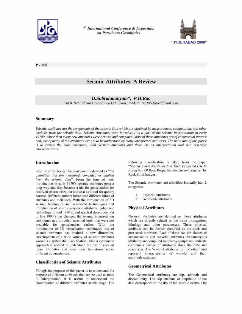
(a)

(b)Fig.1. Normal seismic section (a) showing high amplitude anomaly at shallow depth (b) showing the amplitude attribute of the same section. Notice the High amplitude anomaly is highlighted more clearly in amplitude envelope

Envelope Derivative (RE)This is the time derivative of the envelope.

RE(t)=dE(t)/dtThe derivative of envelope highlights the

change in reflectivity and is also related to the absorption of energy.

Sharpness of the rise time relates to absorption

sharp interfaces Shows discontinuities,

It is used in computation of group propagation direction. When compared with phase propagation direction, it may indicate dispersive waves

Second Derivative of Envelope (DDE)This is given by:

DDE(t)=d2E(t)/dt2

The second derivative of the envelope highlights the interfaces very well - the places of change. This attribute is not too sensitive to the amplitude and can highlight even weak events.

Amplitude Anomaly

Shows all reflecting interfaces visible within seismic band-width

Shows sharpness of events Indicates sharp changes of lithology Large changes of the depositional

environment, even corresponding envelope amplitude may be low.

Very good presentation of image of the subsurface within the seismic bandwidth

Instantaneous Phase

Instantaneous phase attribute is given by (t)=arc tan |H(t)/T(t)|The seismic trace T(t) and its Hilbert transform H(t) are related to the envelope E(t) and the phase (t) by the following relation:T(t)=E(t)cos((t))H(t)=E(t)sin((t))Instantaneous phase is measured in degrees (-, ). It is independent of amplitude and shows continuity and discontinuity of events. It shows bedding very well.Phase along horizon should not change in principle, changes can arise if there is a picking problem, or if the layer changes laterally due to “sink-holes” or other phenomena.This attribute is useful as

Best indicator of lateral continuity, Relates to the phase component of the wave-

propagation. Can be used to compute the phase velocity, Has no amplitude information, hence all

events are represented, Shows discontinuities, but may not be the

best. It is better to show continuities Sequence boundaries,

Detailed visualization of bedding configurations,

Used in computation of instantaneous frequency and acceleration

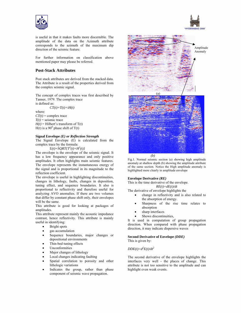
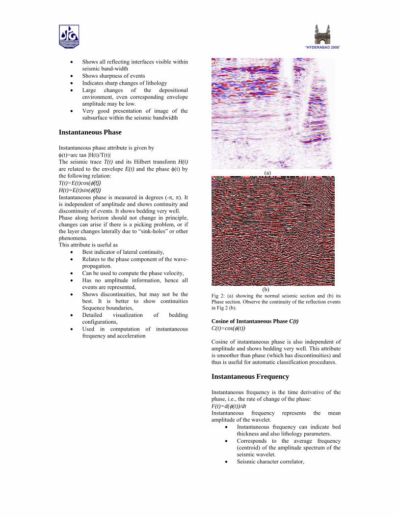
(a)

(b)Fig 2: (a) showing the normal seismic section and (b) its Phase section. Observe the continuity of the reflection events in Fig 2 (b).

Cosine of Instantaneous Phase C(t)C(t)=cos((t))

Cosine of instantaneous phase is also independent of amplitude and shows bedding very well. This attribute is smoother than phase (which has discontinuities) and thus is useful for automatic classification procedures.

Instantaneous Frequency

Instantaneous frequency is the time derivative of the phase, i.e., the rate of change of the phase:F(t)=d((t))/dtInstantaneous frequency represents the mean amplitude of the wavelet.

Instantaneous frequency can indicate bed thickness and also lithology parameters.

Corresponds to the average frequency (centroid) of the amplitude spectrum of the seismic wavelet.

Seismic character correlator,

Indicates the edges of low impedance thin beds,

Hydrocarbon indicator by low frequency anomaly. This effect is some times accentuated by the

Unconsolidated sands due to the oil content of the pores.

Fracture zone indicator, appear as lower frequency zones

Chaotic reflection zone indicator, Bed thickness indicator. Higher frequencies

indicate sharp interfaces or thin shale bedding, lower frequencies indicate sand rich bedding.

Sand/Shale ratio indicator

(a)

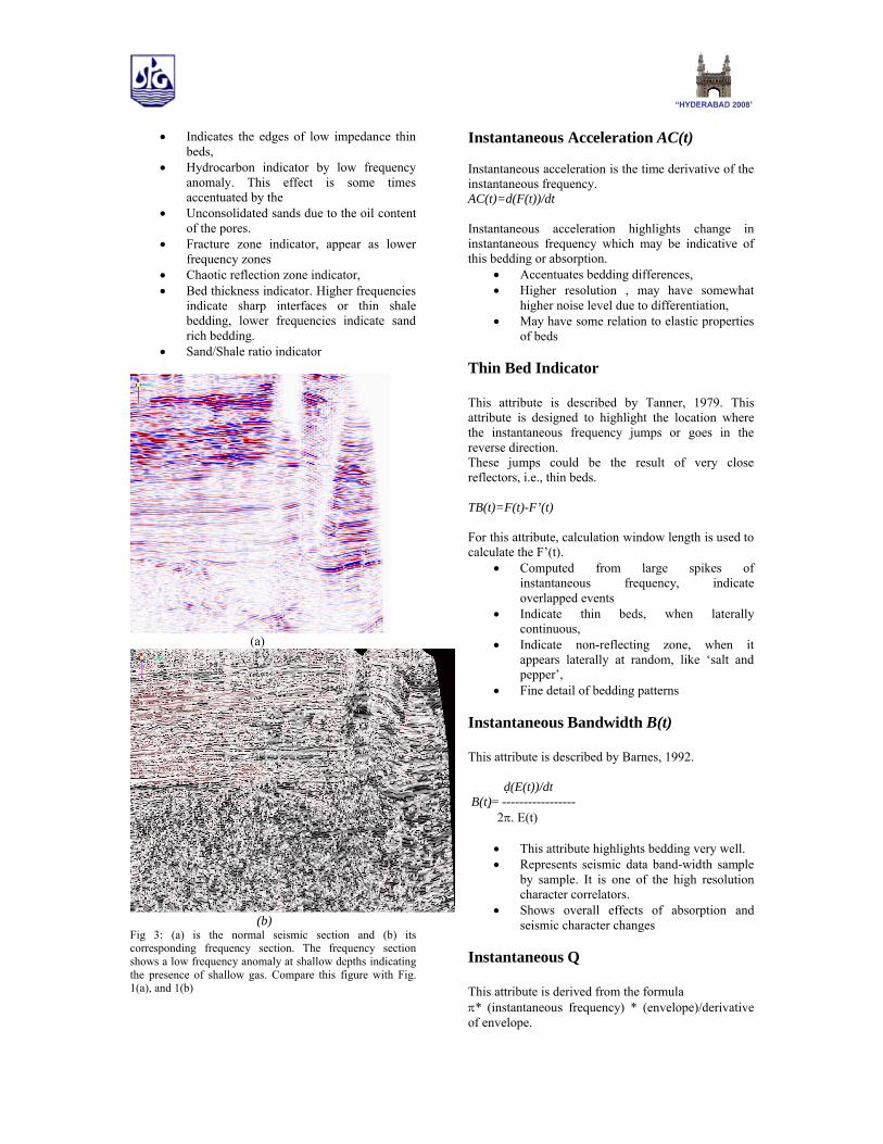
(b)Fig 3: (a) is the normal seismic section and (b) its corresponding frequency section. The frequency section shows a low frequency anomaly at shallow depths indicating the presence of shallow gas. Compare this figure with Fig. 1(a), and 1(b)

Instantaneous Acceleration AC(t)

Instantaneous acceleration is the time derivative of the instantaneous frequency.AC(t)=d(F(t))/dt

Instantaneous acceleration highlights change in instantaneous frequency which may be indicative of this bedding or absorption.

Accentuates bedding differences, Higher resolution , may have somewhat

higher noise level due to differentiation, May have some relation to elastic properties

of beds

Thin Bed Indicator

This attribute is described by Tanner, 1979. This attribute is designed to highlight the location where the instantaneous frequency jumps or goes in the reverse direction.These jumps could be the result of very close reflectors, i.e., thin beds.

TB(t)=F(t)-F’(t)

For this attribute, calculation window length is used to calculate the F’(t).

Computed from large spikes of instantaneous frequency, indicate overlapped events

Indicate thin beds, when laterally continuous,

Indicate non-reflecting zone, when it appears laterally at random, like ‘salt and pepper’,

Fine detail of bedding patterns

Instantaneous Bandwidth B(t)

This attribute is described by Barnes, 1992.

d (E(t))/dtB(t)= -----------------

2. E(t)

This attribute highlights bedding very well. Represents seismic data band-width sample

by sample. It is one of the high resolution character correlators.

Shows overall effects of absorption and seismic character changes

Instantaneous Q

This attribute is derived from the formula* (instantaneous frequency) * (envelope)/derivative of envelope.

Instantaneous Q is an attribute suggested by Barnes. Q is the quality factor that is related to attenuation. Instantaneous Q measures the high frequency component of Q and shows local variations of Q.

Indicates local variation of Q factor, similar to the relative acoustic impedance computation from the seismic trace. Longer wavelength variation should be computed by spectral division and added to this attribute.

May indicate liquid content by ratioing pressure versus shear wave section Q factors.

Indicate relative absorption characteristics of beds

Relative Acoustic Impedance

This attribute calculates the running sum of the trace to which a low cut filter is applied. It is an indicator of impedance changes, in a relative sense. The low cut filter is applied to remove DC shift which is typical in impedance data. (If the value of the low cut filter is zero, then it is not applied.). The calculated trace is the result of simple integration of the complex trace. It represents the approximation of the high frequency component of the relative acoustic impedance.

(a)

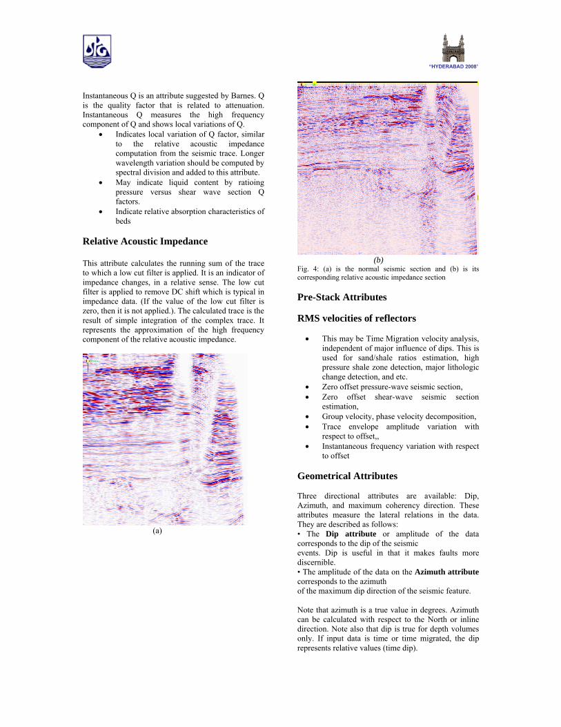
(b)Fig. 4: (a) is the normal seismic section and (b) is its corresponding relative acoustic impedance section

Pre-Stack Attributes

RMS velocities of reflectors

This may be Time Migration velocity analysis, independent of major influence of dips. This is used for sand/shale ratios estimation, high pressure shale zone detection, major lithologic change detection, and etc.

Zero offset pressure-wave seismic section, Zero offset shear-wave seismic section

estimation, Group velocity, phase velocity decomposition, Trace envelope amplitude variation with

respect to offset,, Instantaneous frequency variation with respect

to offset

Geometrical Attributes

Three directional attributes are available: Dip, Azimuth, and maximum coherency direction. These attributes measure the lateral relations in the data. They are described as follows:• The Dip attribute or amplitude of the data corresponds to the dip of the seismicevents. Dip is useful in that it makes faults more discernible.• The amplitude of the data on the Azimuth attributecorresponds to the azimuthof the maximum dip direction of the seismic feature.

Note that azimuth is a true value in degrees. Azimuth can be calculated with respect to the North or inline direction. Note also that dip is true for depth volumes only. If input data is time or time migrated, the dip represents relative values (time dip).

The derivation of the directional attribute is done by considering several traces together to reveal the geometry (dip and azimuth) of the beds.

Discontinuity is a geometrical attribute, and measures the lateral relations in the data. It is designed to emphasize the discontinuous events such as faults. High amplitude values on this attribute corresponds to discontinuities in the data, while low amplitude values correspond to continuous features. Discontinuity varies between zero and one , where zero is continuous and one is discontinuous.The derivation of the attribute is done by considering several traces together to reveal the discontinuity (geometry) of the beds.

This attribute can be used in understanding Coherency at maximum coherency direction Minimum coherency direction Event terminations Picked horizons Fault detection Zones of parallel bedding Zones of chaotic bedding Non-reflecting zones Converging and diverging bedding patterns Unconformities

(a)

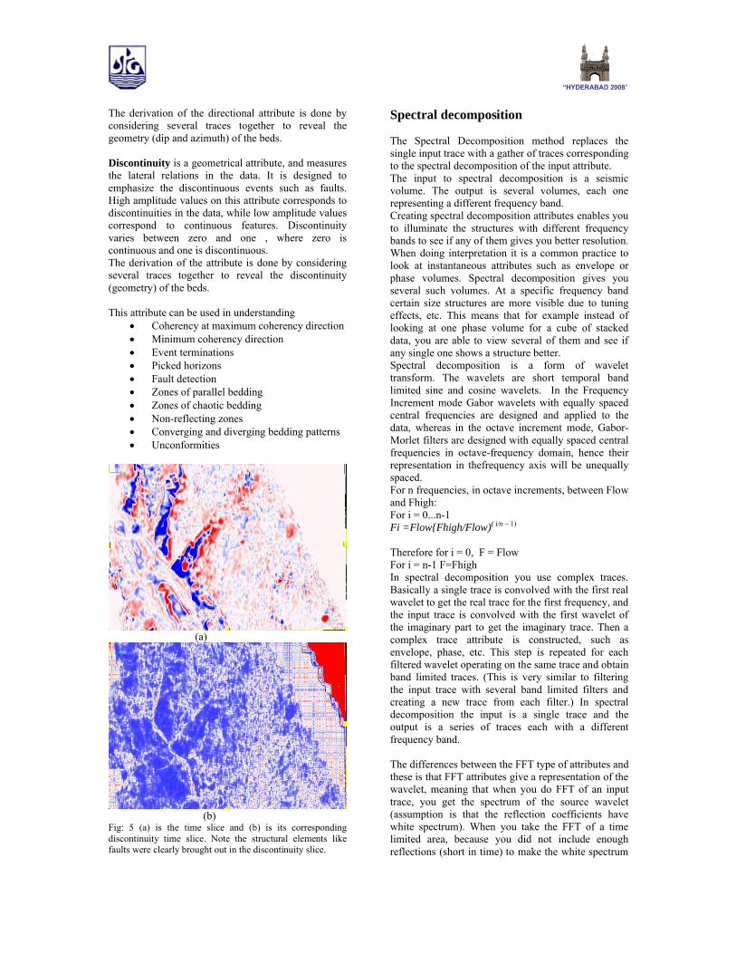
(b)Fig: 5 (a) is the time slice and (b) is its corresponding discontinuity time slice. Note the structural elements like faults were clearly brought out in the discontinuity slice.

Spectral decomposition

The Spectral Decomposition method replaces the single input trace with a gather of traces corresponding to the spectral decomposition of the input attribute.The input to spectral decomposition is a seismic volume. The output is several volumes, each one representing a different frequency band.Creating spectral decomposition attributes enables you to illuminate the structures with different frequency bands to see if any of them gives you better resolution. When doing interpretation it is a common practice to look at instantaneous attributes such as envelope or phase volumes. Spectral decomposition gives you several such volumes. At a specific frequency band certain size structures are more visible due to tuning effects, etc. This means that for example instead of looking at one phase volume for a cube of stacked data, you are able to view several of them and see if any single one shows a structure better. Spectral decomposition is a form of wavelet transform. The wavelets are short temporal band limited sine and cosine wavelets. In the Frequency Increment mode Gabor wavelets with equally spaced central frequencies are designed and applied to the data, whereas in the octave increment mode, Gabor-Morlet filters are designed with equally spaced central frequencies in octave-frequency domain, hence their representation in thefrequency axis will be unequally spaced.For n frequencies, in octave increments, between Flow and Fhigh:For i = 0...n-1Fi =Flow{Fhigh/Flow)( i/n – 1)

Therefore for i = 0, F = FlowFor i = n-1 F=FhighIn spectral decomposition you use complex traces. Basically a single trace is convolved with the first real wavelet to get the real trace for the first frequency, and the input trace is convolved with the first wavelet of the imaginary part to get the imaginary trace. Then a complex trace attribute is constructed, such as envelope, phase, etc. This step is repeated for each filtered wavelet operating on the same trace and obtain band limited traces. (This is very similar to filtering the input trace with several band limited filters and creating a new trace from each filter.) In spectral decomposition the input is a single trace and the output is a series of traces each with a different frequency band.

The differences between the FFT type of attributes andthese is that FFT attributes give a representation of the wavelet, meaning that when you do FFT of an input trace, you get the spectrum of the source wavelet (assumption is that the reflection coefficients have white spectrum). When you take the FFT of a time limited area, because you did not include enough reflections (short in time) to make the white spectrum

assumption, you have the spectrum that is a representation of the reflections coefficients. Also, because you have a limited time window, your resolution in the frequency domain is limited (the shorter the window in time, the wider the frequency band). That is why we refer to frequency bands, rather than frequencies.

Conclusions

This paper discusses about the seismic attributes that are useful as tools for drawing conclusion from the interpretation of seismic data. Though many seismic attributes are available this paper attempts to discuss some of the important attributes. It may be noted that these attributes are very useful tools analysis of a single attribute may not provide a conclusive definitive information. Instead, useful conclusions can be drawn by using a combination of attributes together. Understanding the attribute properties is essential to draw the proper and meaningful conclusions.

Acknowledgements

The authors express their sincere thanks to Sri. D.P. Sahastrabudhe, ED, Basin Manager, Western Onshore Basin, Vadodara for granting the permission to publish the paper.

Suggested Reading:

1. Rock Solid Images, Seismic Attributes and their projected use in prediction of rock properties and seismic facies.

2. Seregey Formel, Local Seismic Attributes,Geophysics, Vol. 72. No.3(May-June 2007); P.A29-A33.

3. M. Turhan Taner, Seismic Attributes, CSEG Recorder, September 2001, P 48-56

4. Satinder Chopra and Kurt Marfurt, Seismic Attributes- A Promising aid for geologic prediction, CSEG Recorder, 2006 Special Edition, P. 110-121

5. Quantitative use of Seismic Attributes for reservoir characterization by Articles from The Leading Edge, October 2002, Vol. 21, No. 10. This Volume contains a Special section on Attributes.

6. Information from different resources and sites from internet.

7. Information from help modules of Paradigm, Landmark and Schlumberger software