Embed Size (px)
Citation preview
This article was originally published in Treatise on Geophysics, Second Edition, published by Elsevier, and the attached copy is provided by Elsevier for the author's benefit and for the benefit of the author's institution, for non-commercial research and educational use including without limitation use in instruction at your institution, sending it to specific colleagues who you know, and providing a copy to your institution’s administrator.
All other uses, reproduction and distribution, including without limitation commercial reprints, selling or licensing copies or access, or posting on open internet sites, your
personal or institution’s website or repository, are prohibited. For exceptions, permission may be sought for such use through Elsevier's permissions site at:
http://www.elsevier.com/locate/permissionusematerial
Mainprice D Seismic Anisotropy of the Deep Earth from a Mineral and Rock Physics Perspective. In: Gerald Schubert (editor-in-chief) Treatise on Geophysics, 2nd edition,
Vol 2. Oxford: Elsevier; 2015. p. 487-538.
Tre
Author's personal copy
2.20 Seismic Anisotropy of the Deep Earth from a Mineral andRock Physics PerspectiveD Mainprice, Universite Montpellier II, Montpellier, France
ã 2015 Elsevier B.V. All rights reserved.
2.20.1 Introduction 4872.20.2 Mineral Physics 4922.20.2.1 Elasticity and Hooke’s Law 4922.20.2.2 Plane Waves and the Christoffel Equation 4942.20.2.3 Measurement of Elastic Constants 5012.20.2.4 Effective Elastic Constants for Crystalline Aggregates 5022.20.2.5 Seismic Properties of Polycrystalline Aggregates at High Pressure and Temperature 5042.20.2.6 Anisotropy of Minerals in the Earth’s Mantle and Core 5062.20.2.6.1 Upper mantle 5062.20.2.6.2 Transition zone 5072.20.2.6.3 Lower mantle 5082.20.2.6.4 Subduction zones 5132.20.2.6.5 Inner core 5182.20.3 Rock Physics 5212.20.3.1 Introduction 5212.20.3.2 Olivine the Most-Studied Mineral: State-of-the-Art-Temperature, Pressure, Water, and Melt 5212.20.3.3 Seismic Anisotropy and Melt 5262.20.4 Conclusions 529Acknowledgments 530References 530
2.20.1 Introduction
Seismic anisotropy is commonly defined as the direction-
dependent nature of the propagation velocities of seismic
waves. However, this definition does not cover all the seismic
manifestations of seismic anisotropy. In addition to direction-
dependent velocity, there is direction-dependent polarization
of P- and S-waves, and anisotropy can contribute to the split-
ting of normal modes. Seismic anisotropy is a characteristic
feature of the Earth, with anisotropy being present near the
surface due to aligned cracks (e.g., Crampin, 1984), in the
lower crust, upper mantle, and lower mantle due to mineral
preferred orientation (e.g., Karato, 1998; Mainprice et al.,
2000). At the bottom of the lower mantle in the D00 layer
(e.g., Kendall and Silver, 1998), and in the solid inner core
(e.g., Ishii et al., 2002a), the causes of anisotropy are still
controversial (Figure 1). In some cases, multiple physical fac-
tors could be contributing to the measured anisotropy, for
example, mineral crystal preferred orientation (CPO) and
alignment of melt inclusions at mid-ocean ridge systems
(e.g., Mainprice, 1997). In the upper mantle, the pioneering
work of Hess (1964) and Raitt et al. (1969) from Pn velocity
measurements in the shallow mantle of the ocean basins
showed azimuthal anisotropy in a shallow horizontal layer.
Long-period surface waves studies (e.g., Montagner and
Tanimoto, 1990; Nataf et al., 1984) have since confirmed
that azimuthal anisotropy and SH/SV polarization anisotropy
are global phenomena in the Earth’s upper mantle, particularly
in the top 200 km of the upper mantle. Anisotropic global
atise on Geophysics, Second Edition http://dx.doi.org/10.1016/B978-0-444-538
Treatise on Geophysics, 2nd edition
tomography, based on surface and body wave data, has
shown that anisotropy is very strong in the subcontinental
mantle and present generally in the upper mantle, but signifi-
cantly weaker at greater depths (e.g., Beghein et al., 2006;
Panning and Romanowicz, 2006). The large wavelengths
used in long-period surface wave studies mean that such
methods are insensitive to heterogeneity less than the wave-
length of about 1000 km. In an effort to address the problem
of regional variations of anisotropy, the splitting of SKS tele-
seismic shear waves that propagate vertically has been exten-
sively used. At continental stations, SKS studies show that the
azimuth of the fast polarization direction is parallel to the
trend of mountain belts (Fouch and Rondenay, 2006; Kind
et al., 1985; Silver, 1996; Silver and Chan, 1988, 1991; Vinnik
et al., 1989). From the earliest observations, it was clear that
the anisotropy in the upper mantle was caused by the CPO of
olivine crystals induced by plastic deformation related to man-
tle flow processes at the geodynamic or plate tectonic scale.
The major cause of seismic anisotropy in the upper mantle
is the CPO caused by plastic deformation. Knowledge of the
CPO and its evolution require well-characterized naturally
deformed samples, experimentally deformed samples, and
numerical simulation for more complex deformation histories
of geodynamic interest. The CPO not only causes seismic
anisotropy but also records some aspects of the deformation
history. Samples of the Earth’s mantle are readily found on the
surface in the form of ultramafic massifs and xenoliths in
basaltic or kimberlitic volcanics and as inclusions in dia-
monds. However, samples from depths greater than 220 km
02-4.00044-0 487, (2015), vol. 2, pp. 487-538
Olivine
Pyrolite
Volume fractions201.00
410
660
2000
2700
2891
5150
6371
1.05 1.10
VSH > VSV
VSH > VSV
VS
V >
VS
H
40 60 80 20 40 60 80Volume fractions Kyanite Wadeite
Orthoclase
Upper mantle
Transition zone
Lower mantle
Pressure (G
Pa)
Temp
erature (C)
Dep
th (km)
Dep
th (k
m)
P-and S-Wave anisotropy MORB Sediments
Cpx CpxCoesite
Stish-ovite
CaAlSi-phase
Ca P
vAl-phase
(CaF Type)
Al-phase(CaF Type)
Liquid iron
ε-phase HCP Iron
x= V 2SH /V 2sv
Fe-Al-M
g Persovskite
Ca P
erovskite
Stishovite
Ca P
ersovskite
Ferropericlase
New Al-phase(hexagonal)
K-Holl andite
RingwooditeWadsleyite
Fe-Al-Mg Perovskite
Fe high spin
?
? ?
?
?
? ?? ?
?
Fe low spin(radiative thermalconductor)
Post-perovskite
Vp N
E
S
W
Opx+Cpx
Garnet+Majorite
Garnet+Majorite
Garnet+Majorite
410 1400 13
660 1600 24
2000 2000 70
2700 2500 125
2891 3000 136
5150 5000 329
6371 5200 364
Inner core
Outer core
CMB
D” Layer
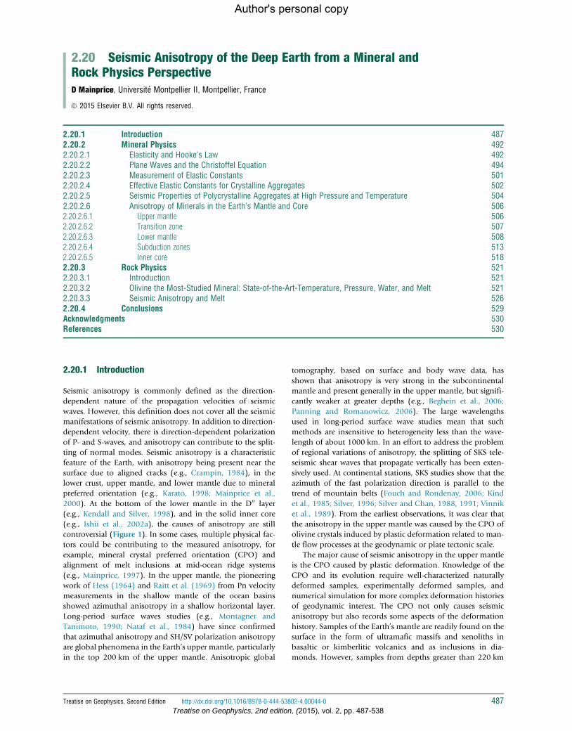
Figure 1 The simplified petrology and seismic anisotropy of the Earth’s mantle and core. The radially (transverse isotropic) anisotropic model of S-waveanisotropy of the mantle is taken from Panning and Romanowicz (2006). The icon at the inner core represents the fast P-wave velocities parallel tothe rotation axis of the Earth. The petrology ofmantle is taken fromOno and Oganov (2005) for pyrolite and Perrillat et al. (2006) and Ricolleau et al. (2010)for the transformed MORB and based on Irifune et al. (1994) as modified by Poli and Schmidt (2002) for the transformed argillaceous sediments.
488 Seismic Anisotropy of the Deep Earth from a Mineral and Rock Physics Perspective
Author's personal copy
are extremely rare. Upper mantle samples large enough for the
measurement of CPO have been recovered from kimberlitic
volcanics in South Africa to a depth of about 220 km estab-
lished by geobarometry (e.g., Boyd, 1973). Kimberlite mantle
xenoliths of deeper origin (>300 km) with evidence for equil-
ibrated majorite garnet, which is now preserved as pyrope
garnet with exsolved pyroxene, have been reported (Haggerty
and Sautter, 1990; Sautter et al., 1991). It has been proposed
that the Alpe Arami peridotite garnet lherzolite has been
exhumed from a minimum depth of 250 km based on clin-
oenstatite exsolution lamellae present in diopside grains
(Bozhilov et al., 1999). Samples of even deeper origin are
preserved as inclusions in diamonds. Although most dia-
monds crystallize at depths of 150–200 km, some diamonds
contain inclusions of majorite (Moore and Gurney, 1985),
enstatite and ferropericlase (Scott-Smith et al., 1984), and
CaSiO3+(Fe,Mg)SiO3+SiO2 (Harte and Harris, 1993). The
mineral associations imply transition zone (410–660 km)
and lower mantle origins for these diamond inclusions
(Kesson and Fitz Gerald, 1991). Although these samples help
to constrain mantle petrology, they are too small to provide
information about CPO. Hence, knowledge of CPO in the
transition zone, lower mantle, and inner core will be derived
from deformation experiments at high pressure and
temperature (e.g., olivine (Couvy et al., 2004), ringwoodite
(Karato et al., 1998), perovskite (Cordier et al., 2004b),
MgGeO3 postperovskite (Merkel et al., 2006a), and e-phaseiron (Merkel et al., 2005)).
It has been accepted since the PREM seismic model
(Dziewo�nski and Anderson, 1981) that the top 200 km of the
Treatise on Geophysics, 2nd edition,
Earth’s mantle is anisotropic on a global scale (Figure 1). How-
ever, there are exceptions, for example, under the Baltic shield,
the anisotropy increases below 200 km (Pedersen et al., 2006).
The seismic discontinuity at about 200 kmwas first reported by
the Danish seismologist Lehmann (1959, 1961), which now
bears her name. However, the discontinuity is not always pre-
sent at the same depth. Anderson (1979) interpreted the dis-
continuity as the petrologic change of garnet lherzolite to
eclogite. More recently, interpretations have favored an anisot-
ropy discontinuity, although, even this is controversial (see
Vinnik et al., 2005), proposed interpretations include a local
anisotropic decoupling shear zone marking the base of the
lithosphere (Leven et al., 1981), a transition from an aniso-
tropic mantle deforming by dislocation creep to isotropic man-
tle undergoing diffusion creep (Karato, 1992), simply the base
of an anisotropic layer beneath continents (e.g., Gaherty and
Jordan, 1995), or the transition from [100] to [001] direction
slip in olivine (Mainprice et al., 2005). Global tomography
studies show that the base of the anisotropic subcontinental
mantle may vary in depth from 100 to 450 km (e.g., Polet and
Anderson, 1995), but most global studies favor an anisotropy
discontinuity for S-waves at around 200–250 km, which is
stronger and deeper (300 km) beneath continents (e.g., Deuss
and Woodhouse, 2002; Panning and Romanowicz, 2006;
Ritsema et al., 2004) and weaker and shallower (200 km)
beneath the oceans. There is also evidence for weak seismic
discontinuities at 260 and 310 km that have been reported in
subduction zones by Deuss and Woodhouse (2002).
A major seismic discontinuity at 410 km is due to the
transformation of olivine to wadsleyite (e.g., Helffrich and
(2015), vol. 2, pp. 487-538
Seismic Anisotropy of the Deep Earth from a Mineral and Rock Physics Perspective 489
Author's personal copy
Wood, 1996) with a shear wave impedance contrast of 6.7%
(e.g., Shearer, 1996). The 410 km discontinuity has topogra-
phy within 5 km of the global average. The olivine to wad-
sleyite transformation will result in the lowering of anisotropy
with depth. Global tomography models (e.g., Beghein et al.,
2006; Montagner, 1994a,b; Montagner and Kennett, 1996;
Panning and Romanowicz, 2006) indicate that the strength
of anisotropy is less in the transition zone (410–660 km)
than in the upper mantle (Figure 1). A global study of the
anisotropy of transition zone by Trampert and van Heijst
(2002) has detected a weak anisotropy shear wave of about
1–2%. The surface wave overtone technique used by Trampert
and van Heijst (2002) cannot localize the anisotropy within
the 410–660 km depth range; however, the only mineral with
a strong anisotropy and significant volume fraction in the
transition zone is wadsleyite occurring between 410 and
520 km. Between 520 and 660 km, there is an increase in the
very weakly anisotropic phases, such as garnet, majorite, and
ringwoodite in the transition zone (Figure 1). Tommasi et al.
(2004) had shown that the CPO predicted by a plastic flow
model using the experimentally observed slip systems of wad-
sleyite can reproduce the weak anisotropy observed by
Trampert and van Heijst (2002). The weaker discontinuity at
520 km, with a shear wave impedance contrast of 2.9%, has
been reported by Shearer and coworkers (e.g., Flanagan and
Shearer, 1998; Shearer, 1996). The discontinuity at 520 km
depth has been attributed to the wadsleyite to ringwoodite
transformation by Shearer (1996). Deuss and Woodhouse
(2001) had reported the ‘splitting’ of the 520 km discontinuity
into two discontinuities at 500 and 560 km, they interpreted
the variations of depth of 520 km, and the presence of two
discontinuities at 500 and 560 km in certain regions can only
be explained by variations in temperature and composition
(e.g., Mg/Mg+Fe ratio), which affect the phase transition Cla-
peyron. Regional seismic studies by Vinnik and coworkers
(Vinnik and Montagner, 1996; Vinnik et al., 1997) show evi-
dence for a weakly anisotropic (1.5%) layer for S-waves at the
bottom 40 km of the transition zone (620–660 km). Some
global tomography models (e.g., Montagner, 1998; Montagner
and Kennett, 1996) also show significant transverse isotropic
anisotropy in the transition zone with VSH>VSV and
VPH>VPV. Given the low intrinsic anisotropy of most of the
minerals in the lower part of the transition zone, Karato (1998)
suggested that this anisotropy is due to petrologic layering
caused by garnet and ringwoodite rich layers of transformed
subducted oceanic crustal material. Such a transversely isotropic
medium with a vertical symmetry axis would not cause any
splitting for vertically propagating S-waves and would not pro-
duce the azimuthal anisotropy observed by Trampert and van
Heijst (2002), but would produce the difference between hori-
zontal and vertical velocities seen by global tomography.
A global study supports this suggestion, as high-velocity slabs
of former oceanic lithosphere are conspicuous structures just
above the 660 kmdiscontinuity in the circum-Pacific subduction
zones (Ritsema et al., 2004). A regional study by Wookey et al.
(2002) also finds significant shear wave splitting associated with
horizontally traveling S-waves, which is compatible with a
layered structure in the vicinity of the 660 km discontinuity.
However, recent anisotropic global tomography models do not
show significant anisotropy in this depth range (Beghein et al.,
2006; Panning and Romanowicz, 2006)
Treatise on Geophysics, 2nd edition
The strongest seismic discontinuity at 660 km is due to the
dissociation of ringwoodite to perovskite and ferropericlase
(Figure 1) with a shear wave impedance contrast of 9.9%
(e.g., Shearer, 1996). The 660 km discontinuity has an impor-
tant topography with local depressions of up to 60 km from
the global average in subduction zones (e.g., Flanagan and
Shearer, 1998). From 660 to 1000 km, a weak anisotropy is
observed in the top of the lower mantle with VSH<VSV and
VPH<VPV (e.g., Montagner, 1998; Montagner and Kennett,
1996). Karato (1998) attributed the anisotropy to the CPO of
perovskite and possibly ferropericlase caused by plastic defor-
mation in the convective boundary layer at the top of the lower
mantle. In this depth range, Kawakatsu and Niu (1994) had
identified a flat seismic discontinuity at 920 km with S to
P converted waves with an S-wave velocity change of 2.4% in
Tonga, Japan Sea, and Flores Sea subduction zones. They sug-
gested that some sort of phase transformation thermodynam-
ically controls this feature, or alternatively, we may suggest that
it marks the bottom of the anisotropic boundary layer pro-
posed by Montagner (1998) and Karato (1998). Reflectors in
lower mantle have been reported by Deuss and Woodhouse
(2001) at 800 km depth under North America and at 1050 and
1150 km beneath Indonesia; they only considered the 800 km
reflector to be a robust result. Karki et al. (1997c) had sug-
gested that the transformation of the highly anisotropic SiO2
polymorph stishovite to CaCl2 structure at 50�3 GPa at room
temperature may be the possible explanation of reflectivity in
the top of the lower mantle. However, according to Kingma
et al. (1995), the transformation would take place at 60 GPa at
lower mantle temperatures in the range 2000–2500 K, corre-
sponding to depth of 1200–1500 km, that is several hundred
kilometers below the 920 km discontinuity. It is highly specu-
lative to suggest that free silica is responsible for the 920 km
discontinuity as a global feature as proposed by Kawakatsu and
Niu (1994). Ringwood (1991) suggested that 10% stishovite
would be present from 350 to 660 km in subducted oceanic
crust and this would increase to about 16% at 730 km. Hence,
in the subduction zones studied by Kawakatsu and Niu (1994),
it is quite possible that significant stishovite could be present to
1200 km and may be a contributing factor to the seismic
anisotropy of the top of the lower mantle. From 1000 to
2700 km, the lower mantle is isotropic for body waves or free
oscillations (e.g., Beghein et al., 2006; Montagner and Kennett,
1996; Panning and Romanowicz, 2006). Karato et al. (1995)
had suggested by comparison with deformation experiments of
fine-grained analogue oxide perovskite that the seismically
isotropic lower mantle is undergoing deformation by super-
plasticity or diffusive creep, which traditionally has been con-
sidered to not produce a CPO; this is now being challenged by
recent experimental results (Miyazaki et al., 2013; Sundberg
and Cooper, 2008). In the bottom of the lower mantle, the D00
layer (100–300 km thick) appears to be transversely isotropic
with a vertical symmetry axis characterized by VSH>VSV
(Figure 1) (e.g., Kendall and Silver, 1996, 1998), which may
be caused by CPO of the constituent minerals, shape preferred
orientation of horizontally aligned inclusions, possibly melt
(e.g., Berryman, 2000; Williams and Garnero, 1996) or core
material. It has been suggested that the melt fraction of D00 may
be as high as 30% (Lay et al., 2004). Seismology has shown
that D00 is extremely heterogeneous as shown by globally high
fluctuations of shear (2–3%) and compressional (1%) wave
, (2015), vol. 2, pp. 487-538
490 Seismic Anisotropy of the Deep Earth from a Mineral and Rock Physics Perspective
Author's personal copy
velocities (e.g., Lay et al., 2004; Megnin and Romanowicz,
2000; Ritsema and van Heijst, 2001), a variation of the thick-
ness of D00 layer between 60 and 300 km (e.g., Sidorin et al.,
1999a), P- and S-wave velocity variations sometimes correlated
and sometimes anticorrelated (thermal, chemical, and melting
effects?) (e.g., Lay et al., 2004), ultralow-velocity zones at the
base of D00 with Vp 10% slower and Vs 30% slower than
surrounding material (e.g., Garnero et al., 1998), and regions
with horizontal (e.g., Kendall, 2000; Kendall and Silver, 1998)
or inclined anisotropy (e.g., Garnero et al., 2004; Maupin et al.,
2005; McNamara et al., 2003; Wookey et al., 2005a) in the
range 0.5–1.5% and isotropic regions, localized patches of
shear velocity discontinuity, that even predicted the possibility
of a globally extensive phase transformation (Nataf and
Houard,1993) and its Clapeyron slope (Sidorin et al.,
1999b). Until recently, the candidate phase for this transition
was SiO2 (Murakami et al., 2004). However, the mineralogical
picture of the D00 layer has been completely changed with the
discovery of postperovskite by Murakami et al. (2004), which
is produced by the transformation of Mg-perovskite in the
laboratory at pressures greater than 125 GPa at high tempera-
ture. Seismic modeling of the D00 layer using the new phase
diagram and elastic properties of perovskite and postperovskite
can explain many features mentioned earlier near the core–
mantle boundary (Wookey et al., 2005b). The imaging of the
layered structures within the D00 region by van der Hilst et al.
(2007) using three-dimensional inverse scattering of core-
reflected shear waves has provided a more quantitative view
of D00 heterogeneity. The layered structures imaged by van der
Hilst et al. (2007) are compatible with transverse isotropic
anisotropy reported by earlier studies (e.g., Kendall, 2000;
Kendall and Silver, 1998; Wookey et al., 2005a).
Although the outer core was discovered by British geologist
Richard Oldham in 1906 (Oldham, 1906), the inner solid core
was identified 30 years later by the Danish seismologist Inge
Lehmann in a paper published in 1936 with the short title P0.She identified P-waves that traveled through the core region
(PKP, where K stands for core) at epicentral distances of 105–
142� in contradiction to the expected travel times for a single
core model (Lehmann, 1936). She proposed a two-shell model
for the core with a uniform velocity of about 10 km s�1 with a
small velocity discontinuity between each shell and an inner
shell radius of 1400 km, close to the actually accepted value of
1221.5 km from PREM (Dziewo�nski and Anderson, 1981).
The liquid nature of the outer core was first proposed by
Jeffreys (1926) based on shear wave arrival times, and the
solid nature of inner core was first proposed by Birch (1940)
based on the compressibility of iron at high pressure. Given the
great depth (5149.5 km) and the number of layers a seismic
wave has to traverse to reach the inner core and return to the
surface, it is not surprising that the first report of anisotropy of
the inner core was inferred 50 years after the discovery of the
inner core. Poupinet et al. (1983) were the first to observe that
PKIKP (where K now stands for the outer core and I is for inner
core) P-waves travel about 2 s faster parallel to the Earth’s
rotation axis than waves traveling the equatorial plane. They
interpreted their observations in terms of a possible heteroge-
neity of the inner core. Shortly afterward, a PKIKP travel time
study by Morelli et al., 1986 and normal modes (free oscilla-
tions) by Woodhouse et al. (1986) reported new observations
Treatise on Geophysics, 2nd edition,
and interpreted the results in terms of anisotropy. However,
the interpretation of PKIKP body wave travel times in terms of
anisotropy remained controversial, with an alternative inter-
pretation being that the inner core had a nonspherical structure
(e.g., Widmer et al., 1992). Finally, the observation of large
differential travel times for PKIKP for paths from the South
Sandwich Islands to Alaska by Creager (1992) and Song and
Helmberger (1993) and the interpretation of higher-quality
free oscillation data by Tromp (1993,1994) and Durek and
Romanowicz (1999) gave further strong support for the
homogenous transverse anisotropy interpretation. The general
consensus became that the inner core is strongly anisotropic,
with a P-wave anisotropy of about 3–4% with the fast velocity
direction parallel to the Earth’s rotation axis (see reviews by
Creager, 2000; Song, 1997; Tromp, 2001). However, many
studies have suggested variations to this simple anisotropy
model of the inner core. It has been suggested that the symme-
try axis of the anisotropy is tilted from the Earth’s rotation axis
(Creger, 1992; Shear and Toy, 1991; Su and Dziewo�nski, 1995)
by 5–10�. A significant difference in the anisotropy between
eastern and western hemispheres of the inner core has been
reported by Creger (1999) and Tanaka and Hamaguchi (1997)
with the western hemisphere having significantly stronger
anisotropy than the eastern hemisphere that is nearly isotropic.
Several recent studies concur that the outer part (100–200 km)
of the inner core is isotropic and inner part is anisotropic (e.g.,
Garcia, 2002; Garcia and Souriau, 2000, 2001; Song and
Helmberger, 1998; Song and Xu, 2002; Sun and Song, 2008).
It has also been suggested that there is a small innermost inner
core with radius of about 300 km with distinct transverse
isotropy relative to the outermost inner core by Ishii and
Dziewo�nski (2002). The innermost core has the slowest P-
wave velocity at 45� to the east–west direction, and the outer
part has a weaker anisotropy with slowest P-wave velocity
parallel to the east–west direction. Using split normal mode
constraints, Beghein and Trampert (2003) also showed that
there is a change in velocity structure with radius in the inner
core; however, their model shows that the symmetry of the P-
and S-wave changes at about 400 km radius, suggesting a rad-
ical change, such as a phase transition of iron. Much of the
complexity of the observations seems to be station- and
method-dependent (see Ishii et al., 2002a,b). In a detailed
study, Ishii et al. (2002a,b) derived a model that simulta-
neously satisfies normal mode, absolute travel time, and dif-
ferential travel time data and has allowed them to separate a
mantle signature and regional structure from global anisotropy
of the inner core. Their preferred model of homogeneous
transverse isotropy with a symmetry axis aligned with the
rotation axis contradicts many of models proposed earlier but
is similar to previous suggestions. In a study of inner core
P-wave anisotropy using both finite-frequency and ray theo-
ries, Calvet et al. (2006) found that the data can be explained
by three families of models that all exhibit anisotropy changes
at a radius between 550 and 400 km (compared to 300 km for
Ishii and Dziewo�nski (2002, 2003) and about 400 km for
Beghein and Trampert (2003)). The first model has a weak
anisotropy with a slow P-wave velocity symmetry axis parallel
to the Earth’s rotation axis. The second model has a nearly
isotropic innermost inner core. Lastly, the third model has a
strongly anisotropic innermost inner core with a fast symmetry
(2015), vol. 2, pp. 487-538
Seismic Anisotropy of the Deep Earth from a Mineral and Rock Physics Perspective 491
Author's personal copy
axis parallel to the Earth’s rotation axis. These models have very
different implications for the origin of the anisotropy and the
history of the Earth’s core. These divergences partly reflect the
uneven sampling of the inner core by PKP(DF) paths resulting
from the spatial distribution of earthquakes and seismographic
stations. A recent study using high-quality, 2360 handpicked
PKIKP arrival times is the largest database to be used for study-
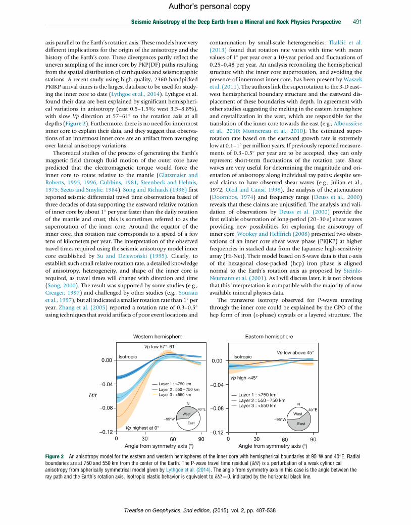
ing the inner core to date (Lythgoe et al., 2014). Lythgoe et al.
found their data are best explained by significant hemispheri-
cal variations in anisotropy (east 0.5–1.5%; west 3.5–8.8%),
with slow Vp direction at 57–61� to the rotation axis at all
depths (Figure 2). Furthermore, there is no need for innermost
inner core to explain their data, and they suggest that observa-
tions of an innermost inner core are an artifact from averaging
over lateral anisotropy variations.
Theoretical studies of the process of generating the Earth’s
magnetic field through fluid motion of the outer core have
predicted that the electromagnetic torque would force the
inner core to rotate relative to the mantle (Glatzmaier and
Roberts, 1995, 1996; Gubbins, 1981; Steenbeck and Helmis,
1975; Szeto and Smylie, 1984). Song and Richards (1996) first
reported seismic differential travel time observations based of
three decades of data supporting the eastward relative rotation
of inner core by about 1� per year faster than the daily rotation
of the mantle and crust; this is sometimes referred to as the
superrotation of the inner core. Around the equator of the
inner core, this rotation rate corresponds to a speed of a few
tens of kilometers per year. The interpretation of the observed
travel times required using the seismic anisotropy model inner
core established by Su and Dziewo�nski (1995). Clearly, to
establish such small relative rotation rate, a detailed knowledge
of anisotropy, heterogeneity, and shape of the inner core is
required, as travel times will change with direction and time
(Song, 2000). The result was supported by some studies (e.g.,
Creager, 1997) and challenged by other studies (e.g., Souriau
et al., 1997), but all indicated a smaller rotation rate than 1� peryear. Zhang et al. (2005) reported a rotation rate of 0.3–0.5�
using techniques that avoid artifacts of poor event locations and
dt/t
Layer 1 : >750 kmLayer 2 : 550- 750 kmLayer 3 : <550 km
Western hemisphere
0 30 60 90-0.12
-0.08
-0.04
0.00
Angle from symmetry axis (°)
Isotropic
Vp low 57°–61°
Vp highest at 0°East
West40 °E
-95°W
N
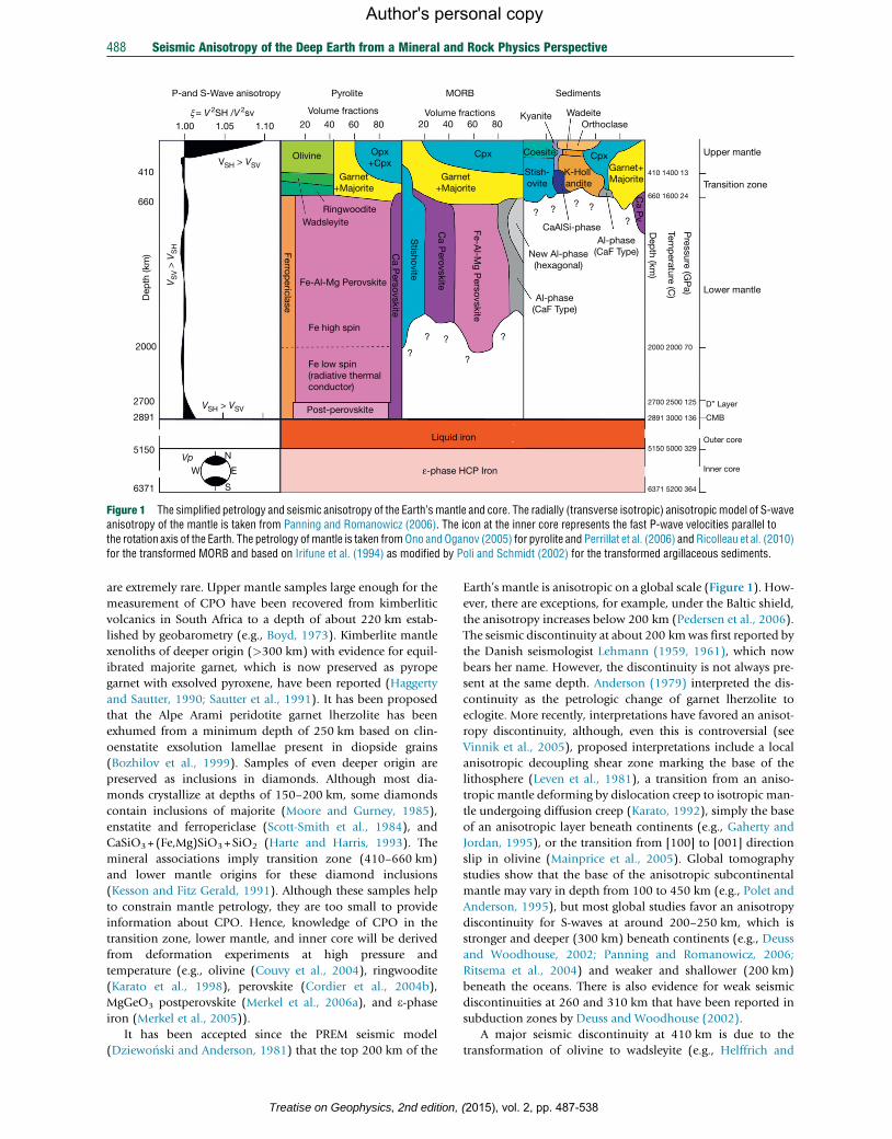
Figure 2 An anisotropy model for the eastern and western hemispheres ofboundaries are at 750 and 550 km from the center of the Earth. The P-waveanisotropy from spherically symmetrical model given by Lythgoe et al. (2014ray path and the Earth’s rotation axis. Isotropic elastic behavior is equivalent
Treatise on Geophysics, 2nd edition
contamination by small-scale heterogeneities. Tkalcic et al.
(2013) found that rotation rate varies with time with mean
values of 1� per year over a 10-year period and fluctuations of
0.25–0.48 per year. An analysis reconciling the hemispherical
structure with the inner core superrotation, and avoiding the
presence of innermost inner core, has been present by Waszek
et al. (2011). The authors link the superrotation to the 3-D east–
west hemispherical boundary structure and the eastward dis-
placement of these boundaries with depth. In agreement with
other studies suggesting the melting in the eastern hemisphere
and crystallization in the west, which are responsible for the
translation of the inner core towards the east (e.g., Alboussiere
et al., 2010; Monnereau et al., 2010). The estimated super-
rotation rate based on the eastward growth rate is extremely
low at 0.1–1� per million years. If previously reportedmeasure-
ments of 0.3–0.5� per year are to be accepted, they can only
represent short-term fluctuations of the rotation rate. Shear
waves are very useful for determining the magnitude and ori-
entation of anisotropy along individual ray paths; despite sev-
eral claims to have observed shear waves (e.g., Julian et al.,
1972; Okal and Cansi, 1998), the analysis of the attenuation
(Doornbos, 1974) and frequency range (Deuss et al., 2000)
reveals that these claims are unjustified. The analysis and vali-
dation of observations by Deuss et al. (2000) provide the
first reliable observation of long-period (20–30 s) shear waves
providing new possibilities for exploring the anisotropy of
inner core. Wookey and Helffrich (2008) presented two obser-
vations of an inner core shear wave phase (PKJKP) at higher
frequencies in stacked data from the Japanese high-sensitivity
array (Hi-Net). Their model based on S-wave data is that c-axis
of the hexagonal close-packed (hcp) iron phase is aligned
normal to the Earth’s rotation axis as proposed by Steinle-
Neumann et al. (2001). As I will discuss later, it is not obvious
that this interpretation is compatible with the majority of now
available mineral physics data.
The transverse isotropy observed for P-waves traveling
through the inner core could be explained by the CPO of the
hcp form of iron (e-phase) crystals or a layered structure. The
Layer 1 : >750 kmLayer 2 : 550-750 kmLayer 3 : <550 km
Eastern hemisphere
0 30 60 90-0.12
-0.08
-0.04
0.00
Angle from symmetry axis (°)
IsotropicVp low above 45°
Vp high <45°
East
40 °E
-95°W
N
West
the inner core with hemispherical boundaries at 95�W and 40�E. Radialtravel time residual (dt/t) is a perturbation of a weak cylindrical). The angle from symmetry axis in this case is the angle between theto dt/t¼0, indicated by the horizontal black line.
, (2015), vol. 2, pp. 487-538
492 Seismic Anisotropy of the Deep Earth from a Mineral and Rock Physics Perspective
Author's personal copy
analysis of the coda of short-period inner core boundary-
reflected P-waves (PKiKP) requires only a few percent heteroge-
neity at length scales of 2 km (Vidale and Earle, 2000), which
suggests a relatively homogenous nonstructured inner core;
however, this interpretation of coda has recently been ques-
tioned by Poupinet and Kennett (2004). The mechanism
responsible for the CPO has been the subject of considerable
speculation in recent years, with the suggested mechanisms
including the alignment of crystals in the magnetic field as
they solidify from the liquid outer core (Karato, 1993), the
alignment of crystals by plastic flow under the action of
Maxwell normal stresses caused the magnetic field (Karato,
1999), faster crystal growth in the equatorial region of the
inner core (Yoshida et al., 1996), anisotropic growth driven by
strain energy (Stevenson, 1987), dendritic crystal growth aligned
with the direction of dominant heat flow (Bergman, 1997),
plastic flow in a thermally convective regime ( Jeanloz and
Wenk, 1988; Wenk et al., 1988, 2000), and plastic flow under
the action of magnetically induced Maxwell shear stresses
(Buffett and Wenk, 2001). An alternative explication that was
proposed by Singh et al. (2000) to explain the P-wave anisot-
ropy and the low shear wave velocity of about 3.6 km s�1
(Deuss et al., 2000) is the presence of a volume fraction of 3–
10% liquid iron (or FeS) in the form of oblate spherical inclu-
sions aligned in the equatorial plane in a matrix of iron crystals
with their c-axes aligned parallel to the rotation axis as originally
proposed by Stixrude and Cohen (1995). The S-wave velocity
and attenuation data are mainly from the outer part of the inner
core, and hence, it was suggested the liquid inclusions are pre-
sent in this region. Note that this is in contradiction with other
studies, which suggest that the outer core has a low anisotropy.
Several problems that are posed by all models to different
degrees are the inner core thermally convective (see Stevenson,
1987; Weber andMachetel, 1992; Yukutake, 1998), the viscosity
of the inner core, the strength of magnetic field and magnitude
Maxwell stresses necessary to cause crystal alignment, the
presence of liquids, and even the ability of the models to cor-
rectly predict the magnitude and orientation of the seismic
P-wave anisotropy. Given the range of seismic models and the
variety of physical phenomena proposed to explain these
models, better contents on the seismic data, probably using
better quality data and a wider geographic distribution of seis-
mic stations in polar regions, are urgently required.
In this chapter, I review our current knowledge of the seismic
anisotropy of the constituent minerals of the Earth’s interior and
our ability to extrapolate these properties to mantle conditions
of temperature and pressure (Figure 1). I will begin by reviewing
the fundamentals of elasticity, plane wave propagation in aniso-
tropic crystals, the measurements of elastic constants, and the
effective elastic constants of crystalline aggregates.
2.20.2 Mineral Physics
2.20.2.1 Elasticity and Hooke’s Law
Robert Hooke’s experiments demonstrated that extension of a
spring is proportional to the weight hanging from it, which was
published in de Potentia Restitutiva (or of Spring Explaining the
Power of Springing Bodies (1678)), establishing that in elastic
solids, there is a simple linear relationship between stress and
Treatise on Geophysics, 2nd edition,
strain. The relationship is now commonly known as Hooke’s
law (Ut tensio, sic vis – which translated from Latin is ‘as is the
extension, so is the force’ – was the solution to an anagram
announced 2 years early in ‘A Description of Helioscopes and
some other Instruments 1676,’ to prevent Hooke’s rivals from
claiming to have made the discovery themselves!). In the case of
small (infinitesimal) deformations, a Maclaurin expansion of
stress as a function of strain developed to first order correctly
describes the elastic behavior of most linear elastic solids:
sij eklð Þ¼ sij 0ð Þ+ @sij@ekl
� �@ekl¼0
ekl +1
2
@sij@ekl@emn
� �@ekl¼0
@emn¼0
eklemn + L
As the elastic deformation is zero at a stress of zero, then
sij(0)¼0, and restricting our analysis to first order, then we
can define the fourth-rank elastic tensor cijkl as
cijkl ¼ @sij@ekl
� �@ekl¼0
where «kl and sij are, respectively, the stress and infinitesimal
strain tensors. Hooke’s law can now be expressed in its tradi-
tional form as
sij ¼ cijkl ekl
The coefficients of the elastic fourth-rank tensor cijkl trans-
late the linear relationship between the second-rank stress and
the infinitesimal strain tensors. The four indexes (ijkl) of the
elastic tensor have values between 1 and 3, so that there are
34¼81 coefficients. The stress tensor is symmetrical as we
assume that stresses acting on opposite faces are equal and
opposite, and hence, there are no stress couples to produce a
net rotation of the elastic material. The infinitesimal strain
tensor is also symmetrical, because we assume that pure and
simple shear quantities are so small that their squares and
products can be neglected. Due to the symmetrical symmetry
of stress and infinitesimal strain tensors, they only have six
independent values rather than nine for the asymmetrical case,
and hence, the first two (i, j) and second two (k,l) indexes of the
elastic tensor can be interchanged:
cijkl cjikl and cijkl ¼ cijlk
The permutation of the indexes caused by the symmetry of
stress and strain tensors reduces the number of independent
elastic coefficients to 62¼36 because the two pairs of indexes
(i,j) and (k,l) can only have six different values:
1� 1, 1ð Þ 2� 2, 2ð Þ 3� 3, 3ð Þ 4� 2, 3ð Þ¼ 3, 2ð Þ 5� 3, 1ð Þ¼ 1, 3ð Þ 6� 1, 2ð Þ¼ 2, 1ð Þ
It is practical to write a 6 by 6 table of 36 coefficients with
two Voigt indexes m and n (cmn) that have values between 1
and 6, whereas the representation of the cijkl tensor with
81 coefficients would be a printer’s nightmare. The relation
between the Voigt (mn) and tensor indexes (ijkl) can be
expressed most compactly by
m¼ diji + 1�dij� �
9� i� jð Þ and n¼ dklk+ 1�dklð Þ 9�k� lð Þwhere dij is the Kronecker delta (dij¼1 when i¼ j and dij¼0
when i 6¼ j).
Combining the first and second laws of thermodynamics
for stress–strain variables, we can define the variation of the
(2015), vol. 2, pp. 487-538
Seismic Anisotropy of the Deep Earth from a Mineral and Rock Physics Perspective 493
Author's personal copy
internal energy (dU) per unit volume of a deformed aniso-
tropic elastic body as a function of entropy (dS) and elastic
strain (deij) at an absolute temperature (T ) as
dU¼ sij deij +TdS
U and S are called state functions. From this equation, it follows
that the stress tensor at constant entropy can be defined as
sij ¼ @U
@eij
� �¼ cijklekl hence cijkl ¼ @sij
@ekl
� �and cklij ¼ @skl
@eij
� �
and finally, we can write the elastic constants in terms of
internal energy and strain as
cijkl ¼ @
@ekl
@U
@eij
� �S
¼ @2U
@eij@ekl
� �S
¼ @2U
@ekl@eij
� �S
¼ cklij
The fourth-rank elastic tensors are referred to as second-
order elastic constants in thermodynamics, because they are
defined as second-order derivatives of a state function (e.g.,
internal energy @2U for adiabatic or Helmholtz free energy @2F
for isothermal constants) with respect to strain; we obtain the
Schwarz integrability condition that allows the interchanging
of the order of partial derivatives of a function. It follows from
these mathematical and thermodynamic arguments that the
symmetry of the derivatives allows the interchange of the first
pair of indexes (ij) with second (kl):
cijkl ¼ cjikl and cijkl ¼ cijlk and now cijkl ¼ cklij
The additional symmetry of cijkl¼ cklij permutation reduces the
number of independent elastic coefficients from 36 to 21, and
tensor with two Voigt indexes is symmetrical, cmn¼ cnm.
Although we have illustrated the case of isentropic (constant
entropy, equivalent to an adiabatic process for a reversible pro-
cess such as elasticity) elastic constants that intervene in the
propagation of elastic waves whose vibration is too fast for
thermal diffusion to establish heat exchange to achieve isother-
mal conditions, these symmetry relations are also valid for
isothermal elastic constants that are used in mechanical prob-
lems. Most of the elastic constants reported in the literature are
determined by the propagation of ultrasonic elastic waves and
are adiabatic. More recently, elastic constants predicted by
atomic modeling for mantle conditions of pressure, and in
some cases temperature, are also adiabatic (see review by Karki
et al., 2001, and also see Chapter 2.08).
The elastic constants in the literature are presented in the
form of 6 by 6 tables for the triclinic symmetry with 21 inde-
pendent values; here, the independent values are shown in
bold characters in the upper diagonal of cmn with the corre-
sponding cijkl:
c11 c12 c13 c14 c15 c16c12 c22 c23 c24 c25 c26c13 c23 c33 c34 c35 c36c14 c24 c34 c44 c45 c46c15 c25 c35 c45 c55 c56c16 c26 c36 c46 c56 c66
6666666664
7777777775¼
c1111 c1122 c1133 c1123 c1113 c1112c1122 c2222 c2233 c2223 c2213 c2212c1133 c2233 c3333 c3323 c3313 c3312c1123 c2223 c3323 c2323 c2313 c2312c1113 c2213 c3313 c2313 c1313 c1312c1112 c2212 c3312 c2312 c1312 c1212
26666664
37777775
In the triclinic system, there are no special relationships
between the constants. On the other extreme is the case of
isotropic elastic symmetry that is defined by just two coeffi-
cients. Note that this is not the same as cubic symmetry, where
there are three coefficients and that a cubic crystal can be
Treatise on Geophysics, 2nd edition
elastically anisotropic. The isotropic elastic constants can be
expressed in the four-index system as
cijkl ¼ ldijdkl +m dikdjl + dildjk� �
where l is Lame’s coefficient and m is the shear modulus. l andm are often referred to as Lame’s constants after the French
mathematician Gabriel Lame, who first published his book
‘Lecons sur la theorie mathematique de l’elasticite des corps
solides’ in 1852. In the two-index Voigt system, the indepen-
dent values are
c11 ¼ c22 ¼ c33 ¼ l +2mc12 ¼ c23 ¼ c13 ¼ lc44 ¼ c55 ¼ c66 ¼ 1⁄2 c11� c12ð Þ¼ m
In matrix form, they are written as
c11 c12 c12 0 0 0
c12 c11 c12 0 0 0
c12 c12 c11 0 0 0
0 0 0 1=2 c11� c12ð Þ 0 0
0 0 0 0 1=2 c11� c12ð Þ 0
0 0 0 0 0 1=2 c11� c12ð Þ
66666666666664
77777777777775where the two independent values are c11 and c12. Another
symmetry that is very important in seismology is the trans-
verse isotropic medium (or hexagonal crystal symmetry). In
many geophysical applications of transverse isotropy, the
unique symmetry direction (X3) is vertical and the other
perpendicular elastic axes (X1 and X2) are horizontal and
share the same elastic properties and velocities. It is very
common in seismological papers to use the notation of
Love (1927) for the elastic constants of transverse isotropic
media where
A¼ c11 ¼ c22 ¼ c1111 ¼ c2222C¼ c33 ¼ c3333F¼ c13 ¼ c23 ¼ c1133 ¼ c2233L¼ c44 ¼ c55 ¼ c2323 ¼ c1313N¼ c66 ¼ 1⁄2 c11�c12ð Þ¼ c1212 ¼ 1⁄2 c1111�c1122ð Þand A�2N¼ c12 ¼ c21 ¼ c11�2c66 ¼ c1212 ¼ c2211 ¼ c1111�2c1212
c11 c12 c13 0 0 0
c12 c11 c12 0 0 0
c13 c13 c33 0 0 0
0 0 0 c44 0 0
0 0 0 0 c44 0
0 0 0 0 0 1=2 c11�c12ð Þ
6666666666664
7777777777775¼
A A�2N F 0 0 0
A�2N A F 0 0 0
F F C 0 0 0
0 0 0 L 0 0
0 0 0 0 L 0
0 0 0 0 0 N
26666666664
37777777775
and the velocities in orthogonal directions that characterize a
transverse isotropic medium are functions of the leading diag-
onal of the elastic tensor and are given as
A¼ c11 ¼ rV2PH C¼ c33 ¼ rV2
PV L¼ c44 ¼ rV2SV N¼ c66
¼ rV2SH
where r is density, VPH and VPV are the velocities of horizon-
tally (X1 or X2) and vertically (X3) propagating P-waves, and
VSH and VSV are the velocities of horizontally and vertically
polarized S-waves propagating horizontally.
Elastic anisotropy can be characterized by taking ratios of
the individual elastic coefficients. Thomsen (1986) introduced
, (2015), vol. 2, pp. 487-538
494 Seismic Anisotropy of the Deep Earth from a Mineral and Rock Physics Perspective
Author's personal copy
three parameters to characterize the elastic anisotropy of any
degree, not just weak anisotropy, for transverse isotropic
medium:
e¼ c11�c33=2c33 ¼A�C=2C
g¼ c66�c44=2c44 ¼N�L=2L
and
d*¼ 1⁄2c233 2 c13 + c44ð Þ2� c33� c44ð Þ c11 + c33�2c44ð Þ� �d*¼ 1⁄2C2 2 F + Lð Þ2� C�Lð Þ A +C�2Lð Þ� �
Thomsen also proposed a weak anisotropy version of the d*parameter:
d¼ c13 + c44ð Þ2� c33�c44ð Þ2=2c33 c33�c44ð Þ� �¼ F + Lð Þ2� C�Lð Þ2=2C C�Lð Þ� �
These parameters go to zero in the case of isotropy and have
values of much less than one (i.e., 10%) in the case of weak
anisotropy. The parameter e describes the P-wave anisotropy
and can be defined in terms of the normalized difference of the
P-wave velocity in the directions parallel to the symmetry axis
(X3, vertical axis) and normal to the symmetry axis (X12,
horizontal plane). The parameter g describes the S-wave anisot-ropy and can be defined in terms of the normalized difference
of the SH wave velocity in the directions normal to the sym-
metry axis (X12, horizontal plane) and parallel to the symme-
try axis (X3, vertical axis) but also in terms SH and SV, because
SH parallel to the symmetry axis has the same velocity as SV
normal to the symmetry axis:
e¼Vp X12ð Þ�Vp X3ð Þ=Vp X3ð Þ¼VPH�VPV=VPV
g¼VSH X12ð Þ�VSH X3ð Þ=VSH X3ð Þ¼VSH X12ð Þ�VSV X12ð Þ=VSV X12ð Þ¼VSH�VSV=VSV
Thomsen (1986) found that the parameter d* controls most
of the phenomena of importance for exploration geophysics,
such as velocities inclined to the symmetry axis (vertical), some
of which are nonnegligible even when the anisotropy is weak.
The parameter d* is an awkward combination of elastic param-
eters, which is totally independent of the velocity in the direction
normal to the symmetry axis (X12 horizontal plane) and which
may be either positive or negative. Mensch and Rosolofosaon
(1997) had extended the application of Thomsen’s parameters
to anisotropic media of arbitrary symmetry and the associated
analysis in terms of the perturbation of a reference model that
can exhibit strong S-wave anisotropy.
In the domain of one- or three-dimensional radial anisotropic
seismic tomography, it has been the practice to use the parameters
f, x, and � to characterize the transverse anisotropy, where
f¼ c33=c11 ¼C=A¼VPV2=VPH
2
x¼ c66=c44 ¼N=L¼VSH2=VSV
2
�¼ c13= c11�2c44ð Þ¼ F= A�2Lð ÞFor characterizing the anisotropy of the inner core, some
authors (e.g., Song, 1997) use a variant of Thomsen’s param-
eters, e 00 ¼(c33�c11)/2c11¼(C�A)/2A (positions of c11 and
c33 reversed from Thomsen; single prime 00 has been added to
avoid confusion here with Thomsen’s parameter),
g¼(c66�c44)/2c44¼(N�L)/2L (same as Thomsen), and
s¼(c11+c33�4c44�2c13)/2c11¼(A+C�4L�2F)/2A (very
Treatise on Geophysics, 2nd edition,
different from Thomsen’s d*); others (e.g., Woodhouse et al.,
1986) use
a¼ c33�c11ð Þ=Ao ¼ C�Að Þ=Ao
b¼ c66�c44ð Þ=Ao
g¼ c11�2c44�c13ð Þ=Ao ¼ A�2N�Fð Þ=Ao
where Ao ¼ roVpo2 is calculated using the density ro and P-wave
velocityVpo at the center of the spherically symmetrical reference
Earth model, PREM (Dziewo�nski and Anderson, 1981). With at
least four different sets of triplets of anisotropy parameters to
describe transverse isotropy in various domains of seismology,
the situations are complex for a researcher who wants to com-
pare the anisotropy from different published works. Even when
comparisons are made, for example, for the inner core (Calvet
et al., 2006), drawing conclusions may be difficult as the
parameters reflect only certain aspects of the anisotropy.
In studying the effect of symmetry of the elastic properties of
crystals, one is directly concerned with only the 11 Laue classes
and not the 32 point groups, because elasticity is a centro-
symmetric physical property. The velocity of an elastic wave
depends on its direction of propagation in an anisotropic crystal,
but not the positive or negative sense of the direction. In this
chapter, we are restricting our study to second-order elastic
constants, corresponding to small strains characteristic of elastic
deformations associated with the propagation of seismic waves.
If we wanted to consider larger finite strains or the effect of an
externally applied stress, we would need to consider third-order
elastic constants, as the approximation adopted in limiting the
components of the strain tensor to terms of the first degree in
the derivatives is no longer justified. For second-order elastic
constants, the two cubic and two hexagonal Laue classes are
not distinct (e.g., Brugger, 1965) andmay be replaced by a single
cubic and a single hexagonal class, which results in only nine
distinct symmetry classes for crystals shown in Table 1.
2.20.2.2 Plane Waves and the Christoffel Equation
There two types of elastic waves, which propagate in an isotro-
pic homogeneous elastic medium, the faster compressional (or
longitudinal) wave with displacements parallel to propagation
direction and slower shear (or transverse) waves with displace-
ments perpendicular to the propagation direction. In aniso-
tropic elastic media, there are three types, one compressional
and two shear waves with in general three different velocities.
In order to understand the displacements associated with dif-
ferent waves and their relationship to the propagation direc-
tion and elastic anisotropy, it is important to consider the
equation of propagation of a mechanical disturbance in an
elastic medium. If we ignore the effect of gravity, we can write
the equation of displacement (ui) as function of time (t) as
r@2ui@t2
� �¼ @sij
@xj
� �
where r is the density and xj is position. From Hooke’s law, we
can see that stress can be written as
sij ¼ cijkl@ul@xk
� �
and hence, elastodynamic equation that describes the inertial
forces can be rewritten with one unknown, the displacement, as
(2015), vol. 2, pp. 487-538
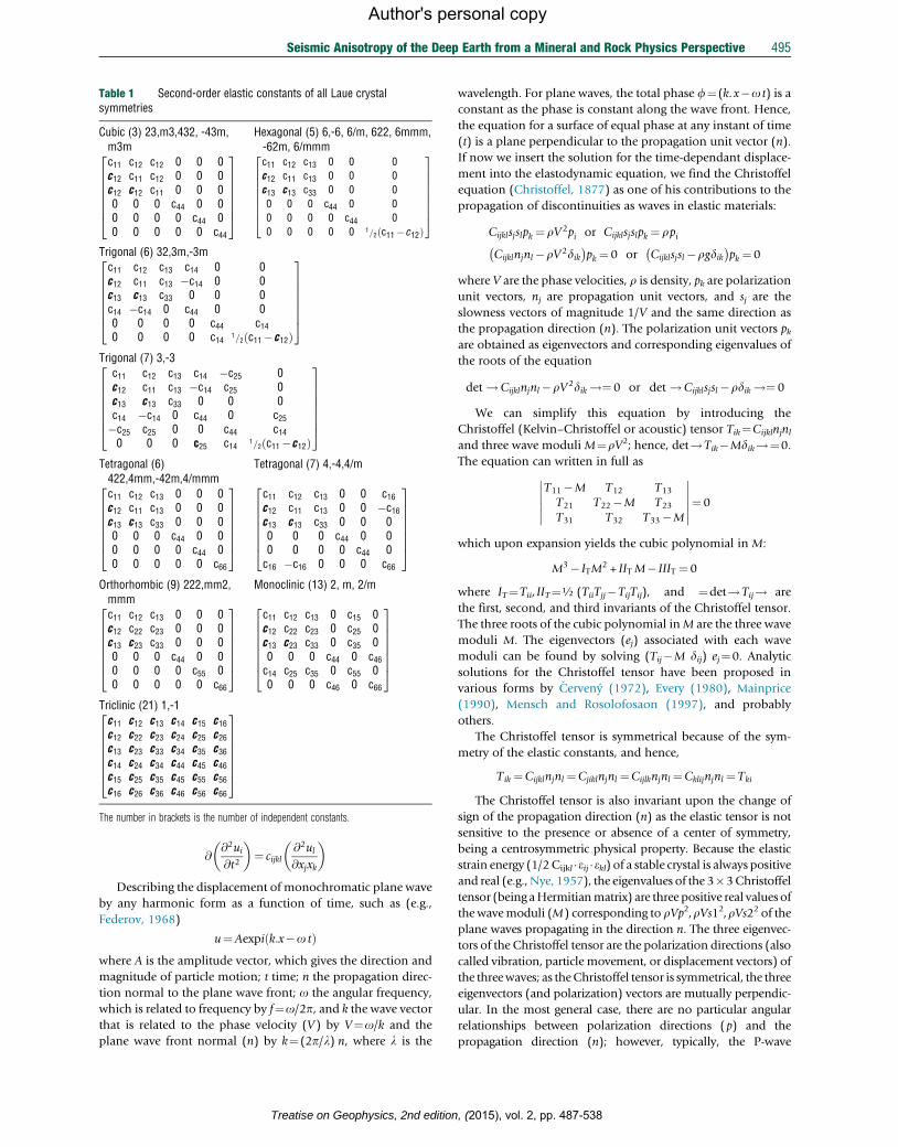
Table 1 Second-order elastic constants of all Laue crystalsymmetries
Cubic (3) 23,m3,432, -43m,m3m
Hexagonal (5) 6,-6, 6/m, 622, 6mmm,-62m, 6/mmm
c11 c12 c12 0 0 0c12 c11 c12 0 0 0c12 c12 c11 0 0 00 0 0 c44 0 00 0 0 0 c44 00 0 0 0 0 c44
26666664
37777775
c11 c12 c13 0 0 0c12 c11 c13 0 0 0c13 c13 c33 0 0 00 0 0 c44 0 00 0 0 0 c44 00 0 0 0 0 1=2 c11� c12ð Þ
266666664
377777775
Trigonal (6) 32,3m,-3mc11 c12 c13 c14 0 0c12 c11 c13 �c14 0 0c13 c13 c33 0 0 0c14 �c14 0 c44 0 00 0 0 0 c44 c140 0 0 0 c14 1=2 c11�c12ð Þ
26666664
37777775
Trigonal (7) 3,-3c11 c12 c13 c14 �c25 0c12 c11 c13 �c14 c25 0c13 c13 c33 0 0 0c14 �c14 0 c44 0 c25�c25 c25 0 0 c44 c140 0 0 c25 c14 1=2 c11�c12ð Þ
26666664
37777775
Tetragonal (6)422,4mm,-42m,4/mmm
Tetragonal (7) 4,-4,4/m
c11 c12 c13 0 0 0c12 c11 c13 0 0 0c13 c13 c33 0 0 00 0 0 c44 0 00 0 0 0 c44 00 0 0 0 0 c66
26666664
37777775
c11 c12 c13 0 0 c16c12 c11 c13 0 0 �c16c13 c13 c33 0 0 00 0 0 c44 0 00 0 0 0 c44 0c16 �c16 0 0 0 c66
26666664
37777775
Orthorhombic (9) 222,mm2,mmm
Monoclinic (13) 2, m, 2/m
c11 c12 c13 0 0 0c12 c22 c23 0 0 0c13 c23 c33 0 0 00 0 0 c44 0 00 0 0 0 c55 00 0 0 0 0 c66
26666664
37777775
c11 c12 c13 0 c15 0c12 c22 c23 0 c25 0c13 c23 c33 0 c35 00 0 0 c44 0 c46c14 c25 c35 0 c55 00 0 0 c46 0 c66
26666664
37777775
Triclinic (21) 1,-1c11 c12 c13 c14 c15 c16c12 c22 c23 c24 c25 c26c13 c23 c33 c34 c35 c36c14 c24 c34 c44 c45 c46c15 c25 c35 c45 c55 c56c16 c26 c36 c46 c56 c66
26666664
37777775
The number in brackets is the number of independent constants.
Seismic Anisotropy of the Deep Earth from a Mineral and Rock Physics Perspective 495
Author's personal copy
@@2ui@t2
� �¼ cijkl
@2ul@xjxk
� �
Describing the displacement of monochromatic plane wave
by any harmonic form as a function of time, such as (e.g.,
Federov, 1968)
u¼Aexpi k:x�o tð Þwhere A is the amplitude vector, which gives the direction and
magnitude of particle motion; t time; n the propagation direc-
tion normal to the plane wave front; o the angular frequency,
which is related to frequency by f¼o/2p, and k the wave vector
that is related to the phase velocity (V) by V¼o/k and the
plane wave front normal (n) by k¼(2p/l) n, where l is the
Treatise on Geophysics, 2nd edition
wavelength. For plane waves, the total phase f¼(k.x�o t) is a
constant as the phase is constant along the wave front. Hence,
the equation for a surface of equal phase at any instant of time
(t) is a plane perpendicular to the propagation unit vector (n).
If now we insert the solution for the time-dependant displace-
ment into the elastodynamic equation, we find the Christoffel
equation (Christoffel, 1877) as one of his contributions to the
propagation of discontinuities as waves in elastic materials:
Cijklsjslpk ¼ rV2pi or Cijklsjslpk ¼ rpi
Cijklnjnl�rV2dik� �
pk ¼ 0 or Cijklsjsl�rgdik� �
pk ¼ 0
where V are the phase velocities, r is density, pk are polarization
unit vectors, nj are propagation unit vectors, and sj are the
slowness vectors of magnitude 1/V and the same direction as
the propagation direction (n). The polarization unit vectors pkare obtained as eigenvectors and corresponding eigenvalues of
the roots of the equation
det !Cijklnjnl�rV2dik !¼0 or det !Cijklsjsl�rdik !¼ 0
We can simplify this equation by introducing the
Christoffel (Kelvin–Christoffel or acoustic) tensor Tik¼Cijklnjnland three wave moduli M¼rV2; hence, det!Tik�Mdik!¼0.
The equation can written in full as
T11�M T12 T13
T21 T22�M T23
T31 T32 T33�M
������������¼ 0
which upon expansion yields the cubic polynomial in M:
M3� ITM2 + IIT M� IIIT ¼ 0
where IT¼Tii, IIT¼½ (TiiTjj�TijTij), and ¼det!Tij! are
the first, second, and third invariants of the Christoffel tensor.
The three roots of the cubic polynomial inM are the three wave
moduli M. The eigenvectors (ej) associated with each wave
moduli can be found by solving (Tij�M dij) ej¼0. Analytic
solutions for the Christoffel tensor have been proposed in
various forms by Cerveny (1972), Every (1980), Mainprice
(1990), Mensch and Rosolofosaon (1997), and probably
others.
The Christoffel tensor is symmetrical because of the sym-
metry of the elastic constants, and hence,
Tik ¼Cijklnjnl ¼Cjiklnjnl ¼Cijlknjnl ¼Cklijnjnl ¼ Tki
The Christoffel tensor is also invariant upon the change of
sign of the propagation direction (n) as the elastic tensor is not
sensitive to the presence or absence of a center of symmetry,
being a centrosymmetric physical property. Because the elastic
strain energy (1/2 Cijkl � eij � ekl) of a stable crystal is always positiveand real (e.g., Nye, 1957), the eigenvalues of the 3�3Christoffel
tensor (being aHermitianmatrix) are three positive real values of
the wavemoduli (M) corresponding to rVp2,rVs12,rVs22 of theplane waves propagating in the direction n. The three eigenvec-
tors of the Christoffel tensor are the polarization directions (also
called vibration, particle movement, or displacement vectors) of
the threewaves; as theChristoffel tensor is symmetrical, the three
eigenvectors (and polarization) vectors are mutually perpendic-
ular. In the most general case, there are no particular angular
relationships between polarization directions (p) and the
propagation direction (n); however, typically, the P-wave
, (2015), vol. 2, pp. 487-538
4
6
8
10
12
14
0 90 180 270
Stishovite
Vp phase VSH phase VSV phase
Pha
se v
eloc
ity (k
ms−1
)
Propagation direction (�)
Vp
VSH
VSV
100 010 100001
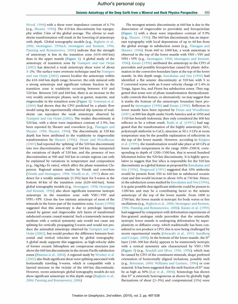
Figure 3 The variation of velocity with direction for tetragonalstishovite as described by Weidner et al. (1982).
496 Seismic Anisotropy of the Deep Earth from a Mineral and Rock Physics Perspective
Author's personal copy
polarization direction is nearly parallel and the two S-wave
polarizations are nearly perpendicular to the propagation direc-
tion and they are termed quasi-P- or quasi-S-waves. If the P-wave
and two S-wave polarizations are, respectively, parallel and per-
pendicular the propagation direction, which may happen along
a symmetry direction, then thewaves are termed pure P and pure
S or pure modes. Only velocities in pure mode directions can be
directly related to single elastic constants (Neighbours and
Schacher, 1967). In general, the three waves have polarizations
that are perpendicular to one another and propagate in the same
direction with different velocities, with Vp>Vs1>Vs2.
A propagation direction for which two (or all three) of the
phase velocities are identical is called an acoustic axis, which
occurs even in crystals of triclinic symmetry. Commonly, the
acoustic axis is associated with the two S-waves having the
same velocity. The S-wave may be identified by their relative
velocity Vs1>Vs2 or by their polarization being parallel to a
symmetry direction or feature, for example, SH and SV, where
the polarization is horizontal and vertical to the third axis of
reference Cartesian frame of the elastic tensor (X3 in the termi-
nology of Nye (1957); X3 is almost always parallel to the crystal
c-axis) in mineral physics and perpendicular to the Earth’s sur-
face in seismology.
What is the difference between an elastic isotopic medium
and an anisotropic medium for wave propagation? For an
isotropic medium, the propagation direction is parallel to the
Vp polarization and the Vs polarizations normal to propagation
direction; all are associatedwith the same S velocity asVs1¼Vs2
and in general Vp>Vs. Even in isotropic medium, the S-wave
polarizations are normal to P-wave polarization. What is differ-
ent for anisotropic medium is that propagation direction is no
longer parallel to theVp polarization by an angle of few degrees,
and the two S-wave polarizations normal to P-wave polariza-
tion are now associated different velocities (Vs1>Vs2). The
angle between propagation direction and the Vp polarization,
as well as the difference between the S-wave velocities, depends
on themagnitude of the elastic anisotropy.While discussing the
difference between isotropic and anisotropic media, it is perti-
nent to mention the case of the ratio between Vp and Vs, which
is a parameter frequentlymeasured in seismology, especially for
regions where fluids may be present. It is a well-known math-
ematical fact that for an isotropic medium, Vp/Vs ratio can be
related to Poisson’s ratio (n) by nonlinear relationship
v¼ 1
2
Vp=Vsð Þ2�2
Vp=Vsð Þ2�1
" #
The mechanical Poisson’s ratio is defined by the negative
radial strain over the longitudinal strain v¼� er/el. Clearly,
Poisson’s ratio does not have any physical connection with
Vp/Vs, which are the velocity of a P-wave with extensional
and contraction strains and that of an S-wave with shear strains
even in the isotropic case; the analogy with anisotropic case is
even less convincing as there are Vs1, Vs2, and Vp where the
polarization strains are inclined to the propagation direction;
and the mechanical situation is very far from Poisson’s ratio.
Hence, I strongly recommend seismologists and rock and min-
eral physicists to report the measurable Vp/Vs1 and Vp/Vs2
ratios of anisotropic media rather than Poisson’s ratio derived
from a calculation of dubious physical significance.
Treatise on Geophysics, 2nd edition,
The velocity at which energy propagates in a homogenous
anisotropic elastic medium is defined as the average power
flow density divided by average total energy density (e.g.,
Auld, 1990) and can be calculated from the phase velocity
using the following relationship given by Federov (1968)
Vie ¼Cijklpjplnk=rV
The phase and energy velocities are related by a vector
equation Vie �ni¼Vi. It is apparent from this relationship that
Ve is not in general parallel to propagation direction (n) and
has a magnitude equal or greater to the phase velocity (V¼o/k). The propagation of waves in real materials occurs as
packets of waves typically having a finite band of frequencies.
The propagation velocity of wave packet is called the group
velocity, and this is defined for plane waves of given finite-
frequency range as
Vig ¼ @w=@kið Þ
The group velocity is in general different to the phase veloc-
ity except along certain symmetry directions. In lossless aniso-
tropic elastic media, the group and energy velocities are
identical (e.g., Auld, 1990); hence, it is not necessary to evaluate
the differential angular frequency versus wave vector to obtain
the group velocity as Vg¼Ve. The group velocity has direct
measurable physical meaning that is not apparent for the
energy or phase velocities.
Various types of plot have been used to illustrate the varia-
tion of velocity with direction in crystals. Velocities measured
by the Brillouin spectroscopy are displayed using graphs of
velocity as a function of propagation directions used in the
experiments. The phase velocities Vp, VSH, and VSV of stishovite
are shown in Figure 3, using the elastic constants from
Weidner et al. (1982); although this type of plot may be useful
for displaying the experimental results, it does not convey the
(2015), vol. 2, pp. 487-538
Seismic Anisotropy of the Deep Earth from a Mineral and Rock Physics Perspective 497
Author's personal copy
symmetry of the crystal. In crystal acoustics, the phase velocity
and slowness surfaces have traditionally illustrated the anisot-
ropy of elastic wave velocity in crystals as a function of the
propagation direction (n) and plots of the wave front (ray or
group) surface given by tracing the extremity of the energy
velocity vector defined earlier. The normal to the slowness
surface has the special property of being parallel to the energy
velocity vector. The normal to the wave front surface has the
special property of being parallel to the propagation (n) and
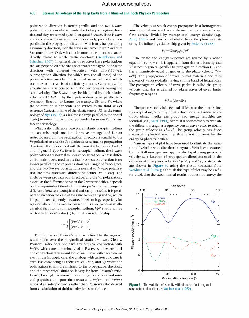
wave vector (k). We can illustrate these polar reciprocal prop-
erties using the elastic constants of the hcp e-phase of iron,
which is considered to be the major constituent of the inner
core, determined by Mao et al. (1998) at high pressure
(Figure 4). Notice that the twofold symmetry along the
a 2110� �
axis of hexagonal e-phase is respected by the slowness
and wave front surfaces of the SHwaves. The wave front surface
can be regarded as a recording after one second of the propa-
gation from a spherical point source at the center of the
0.1 s km −1
Slowness surface
Ve, enevector
n
SH-wave surfaces of e-phase iron
(2110)
(011
(0001)
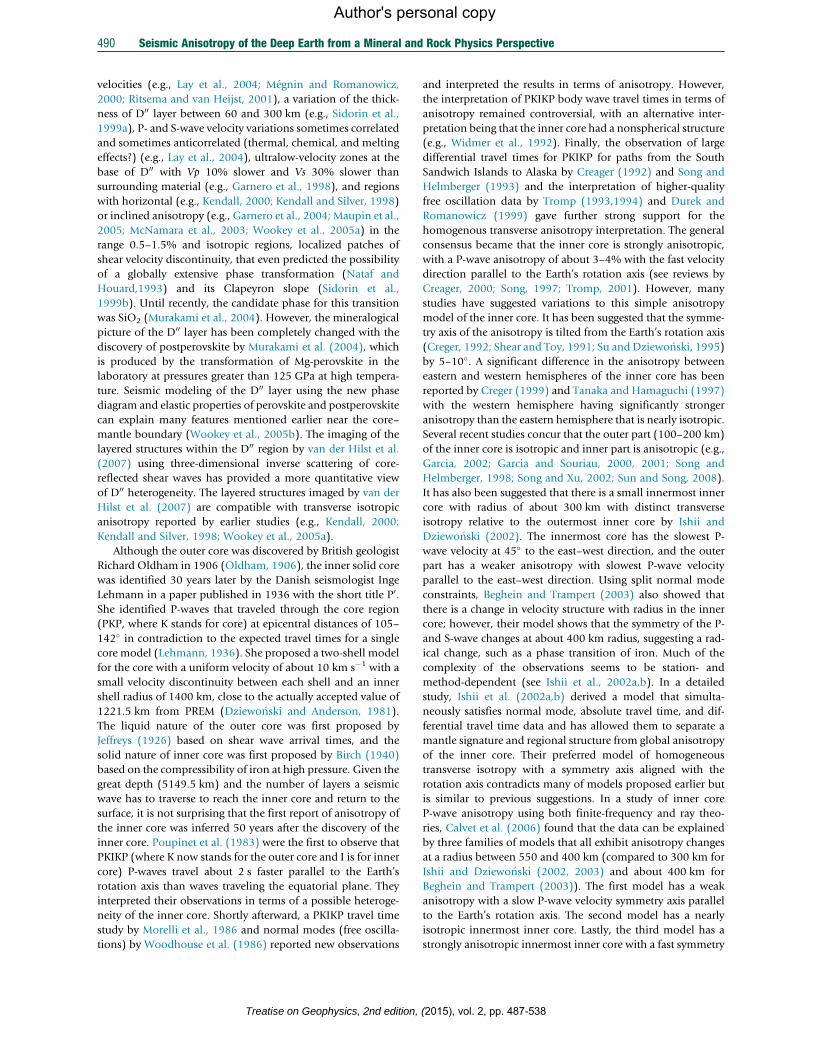
Figure 4 The polar reciprocal relation between the slowness and the waveconstants determined by Mao et al. (1998). The normal to the slowness surfacthe propagation direction (parallel to the wave vector). Note the twofold sym
P
SH
SV
5 km s−1
Min. P =10.28 Max. P =12.16 Min. SH =5.31 Max. SH =8.39 Min. SV =7.66 Max. SV = 7.66
0.1 s km−1
Min. P = 0.08 Min. SH =0.12 Min. SV = 0.13
P
SH
SV
SlownesPhase velocity surface
(100)
(010)
(001)(100)
(0
(0
Stishovite surfac
Figure 5 The three surfaces used to characterize acoustic properties, the pstishovite. Note fourfold symmetry of the surfaces and the cusps on the SH wWeidner et al. (1982) at ambient conditions.
Treatise on Geophysics, 2nd edition
diagram. The wave front is a surface that separates the dis-
turbed from the undisturbed regions. Anisotropic media have
velocities that vary with direction and hence phase velocity and
slowness surfaces with concave and convex undulations in
three dimensions. The undulations are not sharp as velocities
and slowness change slowly with orientation. In contrast, the
wave surface can have sharp changes in direction, called cusps
or folded wave surfaces in crystal physics (e.g., Musgrave,
2003) and triplications or caustics in seismology (e.g.,
Vavrycuk, 2003), particularly for S-waves, which correspond
in orientation to undulations in the phase velocity and slow-
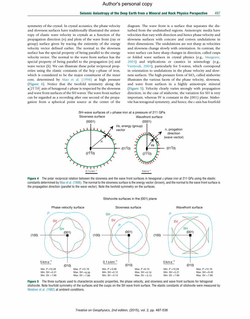
ness surfaces. The high-pressure form of SiO2 called stishovite
illustrates the various facets of the phase velocity, slowness,
and wave front surfaces in a highly anisotropic mineral
(Figure 5). Velocity clearly varies strongly with propagation
direction; in the case of stishovite, the variation for SH is very
important, whereas SV is constant in the (001) plane. Stisho-
vite has tetragonal symmetry, and hence, the c-axis has fourfold
5 km s−1
Wavefront surface
rgy (group)n, progation
direction(wave vector)
Ve
at a pressure of 211 GPa
0)
(2110)
(0110)
(0001)
front surfaces in hexagonal e-phase iron at 211 GPa using the elastice is the energy vector (brown), and the normal to the wave front surface ismetry on the surfaces.
Max. P =0.10 Max. SH =0.19 Max. SV = 0.13
5 km s−1
Min. P =10.28 Max. P =12.16 Min. SH =5.31 Max. SH =9.40 Min. SV = 7.66 Max. SV = 7.66
P
SH
SV
s surface Wavefront surface
10)
01)(100)
(010)
(001)
es in the (001) plane
hase velocity, and slowness and wave front surfaces for tetragonalave front surface. The elastic constants of stishovite were measured by
, (2015), vol. 2, pp. 487-538
498 Seismic Anisotropy of the Deep Earth from a Mineral and Rock Physics Perspective
Author's personal copy
symmetry that can clearly be identified in the various surfaces
in (001) plane. There are orientations where the SH and SV
surfaces intersect, and hence, there is no shear wave splitting
(S-wave birefringence) as both S-waves have the same velocity.
The phase velocity and slowness surfaces have smooth changes
in orientation corresponding to gradual changes in velocity. In
contrast, along the a[100] and b[010] directions, the SH wave
Wavefront cusps on SH-waves in Stishovite in the (001) plane
(100)
(010)
(001)(100)
A
B�
CB
C�
A�
Slowness Wavefront
S
Figure 6 Cusps on the wave front surface of tetragonal stishovite andits relation to the slowness surface in the [100] direction. Thepropagation directions of the wave front are marked by arrows every 10�.See the text for detailed discussion.
e-phase iron (hexagonal) surfac
5 km s−1
5 km s−1
0.1 s km−1
0.1 s km−1
SlownesPhase velocity surface
P SHSV
P
SH
SV
P
SH
SV
10°20°30°40°
50°60°
(000
1) P
lane
(0001) (000
(2110) (211
(0001) (000
(011(0110)
(2110)
(211
0) P
lane
Polarization Energy vector
Polarization Energy vector
Figure 7 Velocity surfaces of e-phase of iron in the second-order prism andisotropic structure. Note the perfectly isotropic (circular) velocity surfaces invelocity surfaces, and for the basal plane, the polarizations for P are normal tS, they are normal and vertical for SV and tangential and horizontal for SH asnormal to the slowness and wave front surfaces in the basal plane.
Treatise on Geophysics, 2nd edition,
front has sharp variations in orientation called cusps. The
cusps on the SH wave front are shown in more detail in
Figure 6, where the cusps on the wave front are clearly related
to minima of the slowness (or maxima on the phase velocity)
surface. The propagation of SH in the a[100] direction is
instructive; if one considers seismometer at the point S, then
seismometer will record first the arrival of wave front AA0, thenBB0, and finally CC0. The parabolic curved nature of the cusp
AA0 is also at the origin of the word caustic to describe this
phenomenon by analogy with the convergent rays in optics,
whereas the word triplication evokes the arrival of the three
wave fronts. Although we are dealing with homogeneous
anisotropic medium, a single crystal of stishovite, the seis-
mometer will record three arrivals for SH, plus of course SV
and P, giving a total of five arrivals for a single mechanical
disturbance. Media with tetragonal elastic symmetry are not
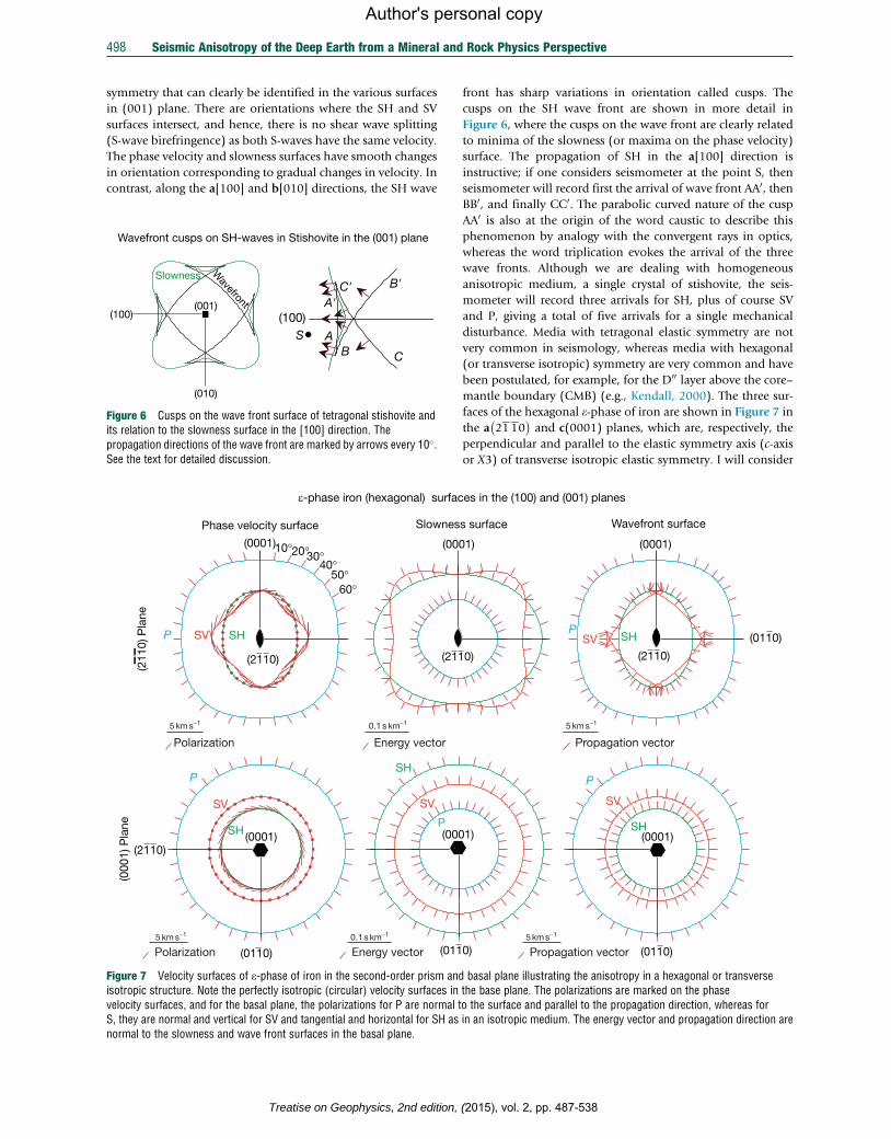
very common in seismology, whereas media with hexagonal
(or transverse isotropic) symmetry are very common and have
been postulated, for example, for the D00 layer above the core–mantle boundary (CMB) (e.g., Kendall, 2000). The three sur-
faces of the hexagonal e-phase of iron are shown in Figure 7 in
the a 2110� �
and c(0001) planes, which are, respectively, the
perpendicular and parallel to the elastic symmetry axis (c-axis
or X3) of transverse isotropic elastic symmetry. I will consider
es in the (100) and (001) planes
5 km s−1
5 km s−1
s surface Wavefront surface
PSHSV
P
SH
SV
1) (0001)
(0110)
0) (2110)
1) (0001)
(0110)0)
Propagation vector
Propagation vector
basal plane illustrating the anisotropy in a hexagonal or transversethe base plane. The polarizations are marked on the phaseo the surface and parallel to the propagation direction, whereas forin an isotropic medium. The energy vector and propagation direction are
(2015), vol. 2, pp. 487-538
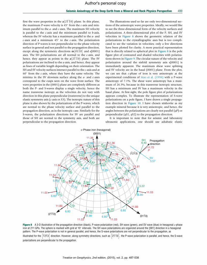
Seismic Anisotropy of the Deep Earth from a Mineral and Rock Physics Perspective 499
Author's personal copy
first the wave properties in the a 2110� �
plane. In this plane,
the maximum P-wave velocity is 45� from the c-axis and min-
imum parallel to the a- and c-axes. The maximum SH velocity
is parallel to the c-axis and the minimum parallel to b-axis,
whereas the SV velocity has a maximum parallel to the a- and
c-axes and a minimum 45� to the c-axis. The polarization
direction of P-waves is not perpendicular to the phase velocity
surface in general and not parallel to the propagation direction,
except along the symmetry directions m 0110� �
and c[0001]
axes. The SH polarizations are all normal to the c-axis, and
hence, they appear as points in the a 2110� �
plane. The SV
polarizations are inclined to the a-axis, and hence, they appear
as lines of variable length depending on their orientation. The
SH and SV velocity surfaces intersect parallel to the c-axis and at
60� from the c-axis, where they have the same velocity. The
minima in the SV slowness surface along the a- and c-axes
correspond to the cusps seen on the wave front surface. The
wave properties in the (0001) plane are completely different as
both the P- and S-waves display a single velocity, hence the
name transverse isotropy as the velocities do not vary with
direction in this plane perpendicular (transverse) to the unique
elastic symmetry axis (c-axis or X3). The isotropic nature of this
plane is also shown by the polarizations of the P-waves, which
are normal to the phase velocity surface and parallel to the
propagation direction, as in the isotropic case. Similarly for the
S-waves, the polarization directions for SV are parallel and
those of SH are normal to the symmetry axis, and both are
perpendicular to the propagation direction.
6.67 6.29
11.36
6.67 6.29
11.36
6.80 6.80
11.07
6.675.22
11.03
6.00
5.29
11.84
6.48
5.72
11.65
5.22 6.80
11.03
6.67 6.29
11.36
6.8
6.6
6.
11.36
5.53
5.89
11.54
5.89 5.35
11.81
5.22
6.80 11.03
6.00
5.29
11.84
5.35
__
ε-Phase iron (hexag
(2110)
(0001)
6.80
Figure 8 A 3-D illustration of the propagation direction (black), P-wave polairon at 211 GPa. The sphere is marked with grid at 10� intervals. The SH wavpattern. The P-wave polarization is not in general parallel, and hence, the S-w
illustrated for the 1213h i
direction. However, along symmetry directions, su
polarizations are perpendicular to the propagation.
Treatise on Geophysics, 2nd edition
The illustrations used so far are only two-dimensional sec-
tions of the anisotropic wave properties. Ideally, we would like
to see the three-dimensional form of the velocity surfaces and
polarizations. A three-dimensional plot of the P, SH, and SV
velocities in Figure 8 shows the geometric relation of the
polarizations to the crystallographic axes but is too compli-
cated to see the variation in velocities; only a few directions
have been plotted for clarity. A more practical representation
that is directly related to spherical plot in Figure 8 is the pole
figure plot of contoured and shaded velocities with polariza-
tions shown in Figure 9. The circular nature of the velocity and
polarization around the sixfold symmetry axis c[0001] is
immediately apparent. The maximum shear wave splitting
and SV velocity are in the basal (0001) plane. From the plot,
we can see that e-phase of iron is very anisotropic at the
experimental conditions of Mao et al. (1998) with a P-wave
anisotropy of 7.1%. The shear wave anisotropy has a maxi-
mum of 26.3%, because in this transverse isotropic structure,
SH has a minimum and SV has a maximum velocity in the
basal plane. At first sight, the pole figure plot of polarizations
appears complex. To illustrate the representation of S-wave
polarizations on a pole figure, I have drawn a single propaga-
tion direction in Figure 10. I have chosen stishovite as my
example mineral because it is very anisotropic, and hence, the
angles between the polarizations are clearly not parallel (qP) or
perpendicular (qS1, qS2) to the propagation direction.
It is important to note that for seismic and laboratory
ultrasonic applications, one should use adiabatic elastic
6.67
6.29
11.36
5.22
6.80 11.03
6.40
5.57
11.72
6.29
11.36
5.89
5.35
11.81
5.22
0 11.03
7
29
5.22
6.80 11.03
6.00
5.29
11.84
5.89
11.81
6.40
5.57
11.72
SH
SV
_ _
_
(1213)P
onal)
(0110)
Propagationdirection
rization (red), SH wave (green), and SV wave (blue) in hexagonal e-phasee polarizations are organized around the [001] direction in a hexagonalave polarizations are not perpendicular to the propagation, as
ch as 21 10h i
, the P-wave polarization is parallel, and hence, the S-wave
, (2015), vol. 2, pp. 487-538
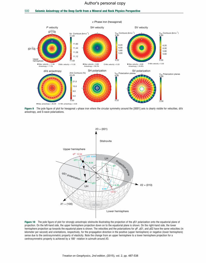
ε-Phase iron (hexagonal)
Upperhemisphere
11.84
11.03
Vp Contours (km s−1)
Max. velocity = 11.84 Anisotropy = 7.1%
Max.velocity = 6.80Anisotropy = 26.3%
Min. velocity = 11.03
Min. anisotropy = 0.00
Min.velocity = 5.22 Min.velocity = 5.30
11.12
11.28
11.44
11.60
26.29
0.00
AVs Contours (%)
Max. anisotropy = 26.29
3.0
9.0
15.0
21.0
6.80
5.22
VSH Polarization planes
6.80
5.22
VSH Contours (km s−1)
Max.velocity = 6.80Anisotropy = 24.8%
5.60 5.80 6.00 6.20
6.80
5.30
VSV Contours (km s−1)
5.60 5.80 6.00 6.20
6.80
5.30
VSV Polarization planes
(0110)
(2110)
P velocity SH velocity SV velocity
dVs anisotropy SH polarization SV polarization
Figure 9 The pole figure of plot for hexagonal e-phase iron where the circular symmetry around the [0001] axis is clearly visible for velocities, dVsanisotropy, and S-wave polarizations.
8.04
6.69
45°
45°
12.54
8.04
6.69 12.54
X3 = (001)
Upper hemisphere
Lower hemisphere
qP qS2
qS1
Stishovite
X1 = (100)
X2 = (010)
qS1 polarization
Projection plane
qS1
qS1
UH
LH
Figure 10 The pole figure of plot for strongly anisotropic stishovite illustrating the projection of the qS1 polarization onto the equatorial plane ofprojection. On the left-hand side, the upper hemisphere projection down on to the equatorial plane is shown. On the right-hand side, the lowerhemisphere projection up towards the equatorial plane is shown. The velocities and the polarizations for qP, qS1, and qS2 have the same velocities (inkilometer per second) and orientations, respectively, for the propagation direction in the positive (upper hemisphere) or negative (lower hemisphere)sense due to the centrosymmetric property of elasticity. Note the change from an upper hemisphere to a lower hemisphere projection for acentrosymmetric property is achieved by a 180� rotation in azimuth around X3.
500 Seismic Anisotropy of the Deep Earth from a Mineral and Rock Physics Perspective
Treatise on Geophysics, 2nd edition, (2015), vol. 2, pp. 487-538
Author's personal copy
Seismic Anisotropy of the Deep Earth from a Mineral and Rock Physics Perspective 501
Author's personal copy
constants, as the timescale of elastic deformation is relatively
short compared with timescale of thermal diffusion. Hence,
thermal diffusion is too slow to obtain isothermal conditions.
We can determine the correction necessary to obtain adiabatic
constants from isothermal ones by considering the elastic
strains caused by stresses and temperature changes:
deij ¼ @eij@skl
� �T
dskl+
@eij@T
� �s@T
In this equation given by Nye (1957), the first term in
brackets on the right-hand side is the elastic compliance tensor
at constant temperature (T ), and the second term is the ther-
mal expansion tensor at constant entropy (s). A second equa-
tion is required to define change in entropy due to changes in
stress and temperature:
dS¼ @S
@skl
� �T
dskl +@S
@T
� �s@T
In this equation, the first term in brackets is the piezocaloric
effect and the second term is heat capacity. If we assume that
entropy is constant (dS¼0) in the second equation and sub-
stitute the result in the first equation, we can eliminate dT and
we obtain
deij ¼ @eij@skl
� �T
dskl� @eij@T
� �s
@S
@skl
� �T
dskl=@T
@S
� �e
Dividing the resulting equation by dskl and using the
relation
@eij@T
� �s¼ @S
@skl
� �T
gives the final result
@eij@skl
� �S
� @eij@skl
� �T
¼� @S
@skl
� �s
@ekl@T
� �s
@T
@S
� �s
¼ @eij@T
� �s
@ekl@T
� �s
@T
@S
� �s
In tensor notation, this is the equation for the difference
between adiabatic and isothermal compliance tensors:
SSijkl�STijkl ¼�aijakl T=Ceð Þ¼�aijakl T=rCPð ÞSSijkl ¼ STijkl�aijakl T=rCPð Þ
where the tensor superscript S stands for adiabatic and T for
isothermal, aij is thermal expansion tensor, T is absolute tem-
perature in Kelvin, Ce is heat capacity per unit volume at
constant strain, CP is specific heat capacity at constant
pressure, and r is density. In a similar way, we can derive the
result for stiffness tensors as
CSijkl ¼CT
ijkl + lijlkl T=rCVð Þl¼ aijCTijkl
where CV is specific heat capacity at constant volume. The
adiabatic stiffness tensor will have greater values than isother-
mal stiffness tensor in general. Stiffness tensors determined by
ab initio modeling in static conditions (T¼0 K) are a special
case as there is no difference between adiabatic and isothermal
tensors. At ambient temperature (T¼300 K), the difference
between adiabatic and isothermal tensors is typically less
than 1%, whereas at 3500 K and 48 GPa, it increases to 7%
Treatise on Geophysics, 2nd edition
for Mg-perovskite (Zhang et al., 2013) and is 13% at 6000 K
and 360 GPa for hcp iron in the inner core (Steinle-Neumann
et al., 2001). For the discussion of the effect of pressure on
these tensors, see Chapter 2.08.
2.20.2.3 Measurement of Elastic Constants
Elastic properties can be measured by a various methods,
including mechanical stress–strain, ultrasonic, Brillouin spec-
troscopy, nonhydrostatic radial x-ray diffraction (RXD), x-ray
and neutron inelastic scattering, and shock measurements.
In addition to physical measurements, atomic-scale first-
principles methods can predict elastic properties of crystals
(see review by Karki et al., 2001; also see Chapter 2.08). The
classical mechanical stress–strain measurements of elastic con-
stants are no longer used due to the large errors, and most
compilations of single-crystal elastic constants (e.g., Anderson
and Isaak, 1995; Bass, 1995; Isaak, 2001) are mainly based on
ultrasonic measurements, the traditional technique at ambient
conditions for large specimens. The measurement of the elastic
constants for minerals from the deep Earth using classical
techniques requires large (�1 cm3) gem quality crystals. How-
ever, many minerals of the deep Earth are not stable, or meta-
stable, at ambient conditions and no large gem quality crystals
are available. Furthermore, the main applications of elastic
constants are for the interpretation of seismological data at
the high-pressure and high-temperature conditions of the
Earth’s mantle and core. Although ultrasonic techniques are
still widely used, new methods are constantly being developed
and refined for measurements at higher pressures and temper-
atures ( Jacobsen et al., 2005; Li et al., 2004; Liebermann and
Li, 1998).
Ultrasonic measurements require a mechanical contact
between the transducers that produce and detect the ultrasonic
signal and the sample. For experiments at high pressure and
temperature, the contact is generally made via the high-
pressure pistons and a high-temperature ceramic buffer rod
or directly with the diamond anvils. Various corrections are
necessary to take into account the ray paths through the pis-
tons and buffer rods and transducer-bond phase shift effects.
The technique most commonly used is based on the ultrasonic
interferometry method introduced by Jackson and Niesler
(1982) to obtain accurate pressure derivatives of single-crystal
MgO to 3 GPa in a piston cylinder apparatus. The use of
ultrasonic interferometry in conjunction with synchrotron
x-radiation in multianvil devices permits a more accurate mea-
surement of elastic constants at simultaneous high pressure
and temperature (Li et al., 2004), as the sample length can be
directly measured by x-radiography in situ, thereby reducing
uncertainties in velocity measurements. A new gigahertz ultra-
sonic interferometer has been recently developed for the dia-
mond anvil cell (DAC; Jacobsen et al., 2005). The gigahertz
frequency reduces the wavelength in minerals to a few
micrometers, which allows the determination of velocity and
the elastic constants for samples of a few tens of micrometers
in thickness. Another ultrasonic technique called resonant
ultrasound spectroscopy has been used to study the elastic
constants of minerals with high precision to very high temper-
atures at ambient pressure (e.g., Isaak, 1992; Isaak et al., 2005).
, (2015), vol. 2, pp. 487-538
502 Seismic Anisotropy of the Deep Earth from a Mineral and Rock Physics Perspective
Author's personal copy
Brillouin scattering spectroscopy has become an established
tool for measuring elastic constants since the introduction of
laser sources and multipass Fabry–Perot interferometers (e.g.,
Vacher and Boyer, 1972). Unlike the ultrasonic techniques that
usually measure the velocity in relatively few crystallographic
directions, and where possible in pure mode directions, using
Brillouin scattering, the velocities can be measured along many
propagation directions and the numerous velocities are inverted
to obtain a least-squares determination of the elastic constants
(Weidner and Carleton, 1977), and hence, it is very suitable for
the measurement of low-symmetry crystals. Brillouin scattering
has several advantages formeasurements of transparentminerals
at high pressure and temperature in a DAC, it only requires a
small sample, no physical contact with the sample is required,
and the Brillouin peaks increase with temperature (Sinogeikin
et al., 2005). The elastic constants ofMgOhave been determined
to high pressure (55 GPa, Zha et al., 2000) and high temperature
(1500 K, Sinogeikin et al., 2005) using Brillouin scattering.
A related technique using laser-induced phonon spectroscopy
in the form of impulsive scattering in a DAC has been used
to measure elastic constants of mantle minerals to 20 GPa (e.g.,
Abramson et al., 1977; Chai et al., 1977a,b).
Several x-ray and neutron diffraction and scattering tech-
niques (e.g., Fiquet et al., 2004) have recently been developed
to explore elastic behavior at extreme pressures (>100 GPa) in
diamond anvils. Experiments using radial RXD of polycrystal-
line samples under nonhydrostatic stress have been used to
estimate the single-crystal elastic constants by using the mea-
sured lattice strains and CPO combined with model polycrys-
talline stress distribution (e.g., Reuss uniform stress field) (e.g.,
Mao et al., 1998, 2008a,b,c; Merkel et al., 2005, 2006b). The
uncertainties in the absolute value of the elastic constants may
be on the order of 10–20%, and model-dependent stress or
strain distributions may be limited by the presence of elastic
and plastic strain in some cases; however, this technique pro-
vides valuable information at extreme pressures. Inelastic x-ray
scattering (IXS) has provided volume-averaged P-wave veloci-
ties of hcp iron as a function of pressures to 112 GPa and
temperatures up to 1100 K (Antonangeli et al., 2004, 2010,
2012; Fiquet et al., 2001). Using knowledge of the CPO com-
bined with different scattering geometries, Antonangeli et al.
(2004) had determined the P-wave velocities in two directions
and C11 elastic constant of hcp iron. The nuclear-resonant IXS
technique provides a direct probe of the phonon density of
states. By the integration of the measured phonon density of
states, the elastic and thermodynamic parameters are obtained,
and when combined with a thermal equation of state (EOS),
the P- and S-wave velocities of hcp iron have been determined
to 73 GPa and 1700 K in a laser-heated DAC by Lin et al.
(2005). However, it has only recently been realized that RXD
and IXS elastic constant or velocity determinations can be
compromised by nonhydrostatic stresses in DACs and the
elastic lattice strain equation is violated by the presence of
plastic strain caused by differential stresses above the plastic
yield stress of the crystals in some cases (Antonangeli et al.,
2006; Mao et al., 2008a,b,c; Merkel et al., 2006b, 2009).
2.20.2.4 Effective Elastic Constants for CrystallineAggregates
The calculation of the physical properties from microstructural
information (crystal orientation, volume fraction, grain shape,
Treatise on Geophysics, 2nd edition,
etc.) is important for upper mantle rocks because it gives
insight into the role of microstructure in determining the
bulk properties and it is also important for synthetic aggregates
experimentally deformed at simulated conditions of the Earth’s
interior. A calculation can be made for the in situ state at high
temperature and pressure of the deep Earth for samples where
the microstructure has been changed by subsequent chemical
alteration (e.g., the transformation from olivine to serpentine)
or mechanically induced changes (e.g., fractures created by
decompression). The in situ temperatures and pressures can
be simulated using the appropriate single-crystal derivatives.
Additional features not necessarily preserved in the recovered
microstructure, such as the presence of fluids (e.g., magma),
can be modeled (e.g., Blackman and Kendall, 1997; Mainprice,
1997; Williams and Garnero, 1996). Finally, the effect of phase
change on the physical properties can also be modeled using
these methods (e.g., Mainprice et al., 1990). Modeling is essen-
tial for anisotropic properties as experimental measurements in
many directions necessary to fully characterize anisotropy are
not currently feasible for the majority of the temperature and
pressure conditions found in the deep Earth.
In the following, we will only discuss the elastic properties
needed for seismic velocities, but the methods apply to all
tensorial properties where the bulk property is governed by the
volume fraction of the constituent minerals. Many properties of
geophysical interest are of this type, for example, thermal con-
ductivity, thermal expansion, elasticity, and seismic velocities.
However, these methods do not apply to properties determined
by the connectivity of a phase, such as the electrical conductivity
of rocks with conductive films on the grain boundaries (e.g.,
carbon). We will assume the sample may be microscopically
heterogeneous due to grain size, shape, orientation, or phase
distribution but will be considered macroscopically uniform.
The complete structural details of the sample are in general
never known, but a ‘statistically uniform’ sample contains
many regions, which are compositionally and structurally
similar, each fairly representative of the entire sample. The
local stress and strain fields at every point r in a linear elastic
polycrystal are completely determined by Hooke’s law as
follows:
sij rð Þ¼Cijkl rð Þ ekl rð Þwhere sij(r) is the stress tensor, Cijkl(r) is the elastic stiffness
tensor, and ekl(r) is the strain tensor at point r. The evaluation
of the effective constants of a polycrystal would be the sum-
mation of all components as a function of position, if we know
the spatial functions of stress and strain. The average stress hsiand strain hei of a statistically uniform sample are linked by an
effective macroscopic modulus C* that obeys Hooke’s law of
linear elasticity:
C*¼ sh i eh i�1
where eh i¼ 1V
ðe rð Þdr and < s>¼ 1
V
ðs rð Þdr where V is the
volume and the notation hi denotes an ensemble average.
The stress s(r) and strain e(r) distribution in a real polycrystal
varies discontinuously at the surface of grains. By replacing the
real polycrystal with a ‘statistically uniform’ sample, we are
assuming that s(r) and strain e(r) are varying slowly and
continuously with position r.
A number of methods are available for determining the
effective macroscopic effective modulus of an aggregate.
(2015), vol. 2, pp. 487-538
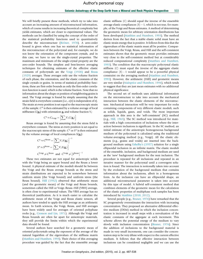
Seismic Anisotropy of the Deep Earth from a Mineral and Rock Physics Perspective 503
Author's personal copy
We will briefly present these methods, which try to take into
account an increasing amount of microstructural information,
which of course results in increasing theoretical complexity but
yields estimates, which are closer to experimental values. The
methods can be classified by using the concept of the order of
the statistical probability functions used to quantitatively
describe the microstructure (Kr€oner, 1978). A zero-order
bound is given when one has no statistical information of
the microstructure of the polycrystal and, for example, we do
not know the orientation of the component crystals, and in
this case, we have to use the single-crystal properties. The
maximum and minimum of the single-crystal property are the
zero-order bounds. The simplest and best-known averaging
techniques for obtaining estimates of the effective elastic
constants of polycrystals are the Voigt (1928) and Reuss
(1929) averages. These averages only use the volume fraction
of each phase, the orientation, and the elastic constants of the
single crystals or grains. In terms of statistical probability func-
tions, these are first-order bounds as only the first-order correla-
tion function is used, which is the volume fraction. Note that no
information about the shape or position of neighboring grains is
used. The Voigt average is found by simply assuming that the
strain field is everywhere constant (i.e., e(r) is independent of r).The strain at every position is set equal to the macroscopic strain
of the sample. C* is then estimated by a volume average of local
stiffnesses C(gi) with orientation gi and volume fraction Vi:
C*CVoigt ¼X
iViC gið Þ
h iReuss average is found by assuming that the stress field is
everywhere constant. The stress at every position is set equal to
the macroscopic stress of the sample. C* or S* is then estimated
by the volume average of local compliances S(gi):
C*CReuss ¼X
iVi S gið Þ
h i�1
S* SReuss ¼X
iVi S gið Þ
h iCVoigt 6¼CReuss and CVoigt 6¼ SReuss
� ��1
These two estimates are not equal for anisotropic solids
with the Voigt being an upper bound and the Reuss a lower
bound. A physical estimate of the moduli should lie between
the Voigt and the Reuss average bounds as the stress and
strain distributions are expected to be somewhere between
uniform strain (the Voigt bound) and uniform stress (the
Reuss bound). Hill (1952) observed that arithmetic mean
(and the geometric mean) of the Voigt and Reuss bounds,
sometimes called the Hill or Voigt–Reuss–Hill (VRH) average,
is often close to experimental values. The VRH average has no
theoretical justification. As it is much easier to calculate the
arithmetic mean of the Voigt and Reuss elastic tensors, all
authors have tended to apply the Hill average as an arithmetic
mean. In Earth sciences, the Voigt, Reuss, and Hill averages
have been widely used for averages of oriented polyphase
rocks (e.g., Crosson and Lin, 1971). Although the Voigt and
Reuss bounds are often far apart for anisotropic materials,
they still provide the limits within which the experimental
data should be found.
Several authors have searched for a geometric mean of
oriented polycrystals using the exponent of the average of the
natural logarithm of the eigenvalues of the stiffness matrix
(Matthies and Humbert, 1993). Their choice of this averaging
procedure was guided by the fact that the ensemble average
Treatise on Geophysics, 2nd edition
elastic stiffness hCi should equal the inverse of the ensemble
average elastic compliances hSi�1, which is not true, for exam-
ple, of the Voigt and Reuss estimates. A method of determining
the geometric mean for arbitrary orientation distributions has
been developed (Matthies and Humbert, 1993). The method
derives from the fact that a stable elastic solid must have an
elastic strain energy that is positive. It follows from this that the
eigenvalues of the elastic matrix must all be positive. Compar-
ison between the Voigt, Reuss, and Hill and the self-consistent
estimates shows that the geometric mean provides estimates
very close to the self-consistent method but at considerably
reduced computational complexity (Matthies and Humbert,
1993). The condition that the macroscopic polycrystal elastic
stiffness hCi must equal the inverse of the aggregate elastic
compliance hSi�1 would appear to be a powerful physical
constraint on the averaging method (Matthies and Humbert,
1993). However, the arithmetic (Hill) and geometric means
are very similar (Mainprice and Humbert, 1994), which tends
to suggest that they are just mean estimates with no additional
physical significance.
The second set of methods uses additional information
on the microstructure to take into account the mechanical
interaction between the elastic elements of the microstruc-
ture. Mechanical interaction will be very important for rocks
containing components of very different elastic moduli, such
as solids, liquids, gases, and voids. The most important
approach in this area is the ‘self-consistent’ (SC) method
(e.g., Hill, 1965). The SC method was introduced for mate-
rials with a high concentration of inclusions where the inter-
action between inclusions is significant. In the SC method, an
initial estimate of the anisotropic homogeneous background
medium of the polycrystal is calculated using the traditional
volume-averaging method (e.g., Voigt). All the elastic ele-
ments (e.g., grains and voids) are inserted into the back-
ground medium using Eshelby’s (1957) solution for a single
ellipsoidal inclusion in an infinite matrix. The elastic moduli
of the ensemble, inclusion, and background medium are used
as the ‘new’ background medium for the next inclusion. The
procedure is repeated for all inclusions and repeated in an
iterative manner for the polycrystal until a convergent solu-
tion is found. The interaction is notionally taken into account
by the evolution of the background medium that contains
information about the inclusions, albeit in a homogenous
form. As the inclusion can have an ellipsoidal shape, an
additional microstructural parameter is taken into account
by this type of model. A hybrid self-consistent method that
combines elements of the geometric mean for the calculation
of the elastic properties of multiphase rock samples has been
introduced by Matthies (2010, 2012).
Several people (e.g., Bruner, 1976) have remarked that the
SC progressively overestimates the interaction with increasing
concentration. They proposed an alternative differential effec-
tive medium (DEM) method in which the inclusion concen-
tration is increased in small steps with a reevaluation of the
elastic constants of the aggregate at each increment. This
scheme allows the potential energy of the medium to vary
slowly with inclusion concentration (Bruner, 1976). Since
the addition of inclusions to the background material is
made in very small increments, one can consider the concen-
tration step to be very dilute with respect to the current effective
medium. It follows that the effective interaction between
inclusions can be considered negligible and we can use the
, (2015), vol. 2, pp. 487-538
504 Seismic Anisotropy of the Deep Earth from a Mineral and Rock Physics Perspective
Author's personal copy
inclusion theory of Eshelby (1957) to take into account the
interaction. In contrast, the SC uses Eshelby’s theory plus an
iterative evaluation of the background medium to take into
account the interaction. Mainprice (1997) had compared the
results of SC and DEM for anisotropic oceanic crustal and
mantle rocks containing melt inclusions and found the results
to be very similar for melt fractions of less than 30%. At higher
melt fractions, the SC exhibits a threshold value around 60%
melt, whereas the DEM varies smoothly up a 100% melt. The
presence of a threshold in the SC calculations is due to the
specific way that the interaction is taken into account. The
estimates of both methods are likely to give relatively poor
results at high fractions of a phase with strong elastic contrast
with the other constituents as other phenomena, such as
mechanical localization related to the percolation threshold,
are likely to occur.
The third set of methods uses higher-order statistical corre-
lation functions to take into account the first- or higher-order
neighbor relations of the various microstructural elements. The
factors that need to be statistically described are the elastic
constants (determined by composition), orientation, and rela-
tive position of an element. If the element is considered to be
small relative to grain size, then grain shape and the heteroge-
neity can be accounted for the relative position correlation
function. Nearest neighbors can be taken into account using
two-point correlation function, which is also called an auto-
correlation function by some authors. If we use the ‘statistically
uniform’ sample introduced earlier, we are effectively assuming
that all the correlation functions used to describe the micro-
structure up to order infinity are statistically isotropic; this is
clearly a very strong assumption. In the special case where all
the correlation functions up to order infinity are defined,
Kr€oner (1978) had shown that the upper and lower bounds
converge for the self-consistent method so that Csc¼(Ssc)�1.
The statistical continuum approach is the most complete
description and has been extensively used for model calcula-
tions (e.g., Beran et al., 1996; Mason and Adams, 1999). Until
recently, it has been considered too involved for practical
application. With the advent of automated determination of
crystal orientation and positional mapping using electron
backscattered diffraction (EBSD) in the scanning electron
microscope (Adams et al., 1993), digital microstructural
maps are now available for the determination of statistical
correlation functions. This approach provides the best possible
estimate of the elastic properties but at the expense of consid-
erably increased computational complexity.
The fact that there is a wide separation in the Voigt and Reuss
bounds for anisotropic materials is caused by the fact that the
microstructure is not fully described by such methods. How-
ever, despite the fact that these methods do not take into
account such basic information as the position or the shape of
the grains, several studies have shown that the Voigt average or
the Hill average is within 5–10% of experimental values for
low-porosity rocks free of fluids. For example, Barruol and Kern
(1996) showed for several anisotropic lower crust and upper
mantle rocks from the Ivrea zone in Italy that the Voigt average
is within 5% of the experimentally measured velocity. Finally,
from a practical point of view, a free and open-source MTEX
toolbox is now available (https://code.google.com/p/mtex/)
for effective medium calculations, such as Voigt, Reuss, and
Treatise on Geophysics, 2nd edition,
Hill averages for second-, third-, and fourth-rank tensors, and,
plotting the results, a wide variety of graphic formats. A detailed
description of the application of MTEX to elastic and seismic
properties can be found in Mainprice et al. (2011).
2.20.2.5 Seismic Properties of Polycrystalline Aggregatesat High Pressure and Temperature
The orientation of crystals in a polycrystal can be measured by
volume diffraction techniques (e.g., x-ray or neutron diffrac-
tion) or individual orientation measurements (e.g., U-stage
and optical microscope, electron channeling, or EBSD). In
addition, numerical simulations of polycrystalline plasticity
also produce populations of crystal orientations at mantle
conditions (e.g., Tommasi et al., 2004). An orientation, often
given the letter g, of a grain or crystal in sample coordinates can
be described by the rotation matrix between crystal and sample
coordinates. In practice, it is convenient to describe the rota-
tion by a triplet of Euler angles, for example, g¼(’1 f ’2)
used by Bunge (1982). One should be aware that there are
many different definitions of Euler angles that are used in the
physical sciences. The orientation distribution function (ODF)
f(g) is defined as the volume fraction of orientations with an
orientation in the interval between g and g+dg in a space
containing all possible orientations given by
DV=V ¼ðf gð Þdg
where DV/V is the volume fraction of crystals with orientation
g, f(g) is the texture function, and dg¼1/8p2 sin f d’1dfd’2
is the volume of the region of integration in orientation space.
To calculate the seismic properties of a polycrystal, one
must evaluate the elastic properties of the aggregate. In the
case of an aggregate with a crystallographic fabric, the anisot-
ropy of the elastic properties of the single crystal must be taken
into account. For each orientation g, the single-crystal proper-
ties have to be rotated into the specimen coordinate frame
using the orientation or rotation matrix gij:
Cijkl gð Þ¼ gip:gjq:gkr :glt Cpqrt goð Þ
where Cijkl(g) is the elastic property in sample coordinates,
gij¼g(’1 f ’2) is the measured orientation in sample co-
ordinates, and Cpqrt(go) is the elastic property in crystal
coordinates.
The elastic properties of the polycrystal may be calculated
by integration over all possible orientations of the ODF. Bunge
(1982) had shown that integration is given as
Cijkl
m¼
ðCijklm gð Þf gð Þdg
where hCijklim is the elastic properties of the aggregate of min-
eral m. Alternatively, it may be determined by simple summa-
tion of individual orientation measurements:
Cijkl
m¼
XCijklm gð Þ:v gð Þ
where v(g) is the volume fraction of the grain in orientation g.
For example, the Voigt average of the rock formmineral phases
of volume fraction v(m) is given as
(2015), vol. 2, pp. 487-538
0.15
0.20
0.25
0.30
0.35
0.40
0.45
0.50
0.55
0 200 400 600 800 1000 1200 1400
Cub
ic a
niso
trop
y fa
ctor
(A)
Temperature (°C)
MgO at 8 GPa
A = ((2C44+ C12)/C11) − 1
dCij /dPdT = 0
Figure 11 An illustration of the importance of the cross pressure–temperature derivatives for cubic MgO at 8 GPa pressure. Withincreasing temperature at constant pressure, the anisotropy measuredby the cubic anisotropy factor (A) increases by a factor of 2. Data fromChen et al. (1998).
Seismic Anisotropy of the Deep Earth from a Mineral and Rock Physics Perspective 505
Author's personal copy
Cijkl
Voigt¼
Xv mð Þ Cijkl
m
The final step is the calculation of the three seismic phase
velocities by the solution of the Christoffel equation, details of
which are given earlier.
To calculate the elastic constants at pressures and
temperatures, the single-crystal elastic constants are given at
the pressure and temperature of their measurement by using
the following relationship:
Cij PTð Þ¼Cij PoToð Þ + dCij=dP� �
DP +1=2 d2Cij=dP2
� �DP2
+ dCij=dT� �
DT + d2Cij=dPdT� �
DPDT
where Cij(PT ) are the elastic constants at pressure P and tem-
perature T, Cij(PoTo) are the elastic constants at a reference
pressure Po (e.g., 0.1 MPa) and temperature To (e.g., 25 �C),dCij/dP is the first-order pressure derivative, dCij/dT is the first-
order temperature derivative, DP¼P�Po, and DT¼T�To. The
equation is a Maclaurin expansion of the elastic tensor as a
function of pressure and temperature, which is a special case of
a Taylor expansion as the series is developed about the elastic
constants at the reference condition Cij(PoTo). The series only
represent the variation of the Cij in their intervals of pressure
and temperature of convergence, in other words the pressure
and temperature range of the experiments or atomic modeling
calculations used to determine the derivatives. Note that this
equation is not a polynomial and care has to be taken when
using the results of data fitted to polynomials, as, for example,
the second-order derivatives fitted to a polynomial should be
multiplied by two for use in the equation mentioned earlier,
for example, second-order pressure derivatives for MgO given
by Sinogeikin et al., (2001). Also note that this equation is not
a Eulerian finite strain EOS (e.g., Davies, 1974; see succeeding
text), and data fit to such an equation will not have derivatives
compatible with the equation mentioned earlier, for example,
the pressure derivatives of brucite determined by Jiang et al.
(2006). The second-order pressure derivatives d2Cij/dP2 are
available for an increasing number of mantle minerals (e.g.,
olivine, orthopyroxene, garnet, and MgO), and the first-order
temperature derivatives seem to adequately describe the tem-
perature dependence of most minerals, although the second-
order derivatives are also available in a few cases (e.g., garnet,
fayalite, forsterite, and rutile; see Isaak, 2001 for references).
Experimental measurements of the cross pressure–temperature
derivatives d2Cij/dPdT (i.e., the temperature derivative of the
Cij/dP at constant temperature) are still very rare. For example,
despite the fact that MgO (periclase) is a well-studied reference
material for high-pressure studies, the complete set of single-
crystal cross derivatives were measured for the first time by
Chen et al. (1998) to 8 GPa and 1600 K. The effect of the
cross derivatives on the Vp and dVs anisotropy of MgO is
dramatic, and the anisotropy is increased by a factor of 2
when cross derivatives are used (Figure 11). Note that when
a phase transition occurs, then the specific changes in elastic
constants at pressures near the phase transition will have to be
taken into account, for example, the SiO2 polymorphs
(Carpenter, 2006; Cordier et al., 2004a; Karki et al., 1997c).
The seismic velocities also depend on the density of the min-
erals at pressure and temperature, which can be calculated
using an appropriate EOS (Knittle, 1995). The Murnaghan
EOS derived from finite strain is sufficiently accurate at
Treatise on Geophysics, 2nd edition
moderate compressions (Knittle, 1995) of the upper mantle
and leads to the following expression for density as a function
of pressure:
r Pð Þ¼ ro 1 + K 0=Kð Þ: P�Poð Þð Þ1=K 0
where K is the bulk modulus, K0 ¼dK/dP is the pressure deriv-
ative of K, and ro is the density at reference pressure Po and
temperature To. For temperature, the density varies as
r Tð Þ¼ ro 1�ðav Tð ÞdT
� � ro 1�aav T�Toð Þ½
where av(T )¼1/V(@V/@T ) is the volume thermal expansion
coefficient as a function of temperature and aav is an average
value of thermal expansion that is constant over the tempera-
ture range (Fei, 1995). According to Watt (1988), an error of
less than 0.4% on the P and S velocity results from using aav to1100 K for MgO. For temperatures and pressures of the mantle,
the density is described for this chapter by
r P, Tð Þ¼ ro 1 + K 0=Kð Þ: P�Poð Þð Þ1=K 01�aav T�Toð Þ½
n oAn alternative approach for the extrapolation elastic con-
stants to very high pressures is Eulerian finite strain theory
(e.g., Davies, 1974). The theory is based on a Maclaurin expan-
sion of the free energy in terms of Eulerian finite volumetric
strain. For example, Karki et al. (2001) reformulated Davies’s
equations for the elastic constants in terms of finite volumetric
strain (f ) as
Cijkl fð Þ¼ 1+2fð Þ7=2 Coijkl + b1f + 1⁄2 b2f + � � �� ��PDijkl
where
f ¼ 1⁄2 Vo=Vð Þ2=3�1h i
b1 ¼ 3Ko dCoijkl=dP� ��5Coijkl
b2 ¼ 9K2o d2Coijkl=dP
2� �
+3 Ko=dPð Þ b1 + 7Coijkl
� ��16b1�49Coijkl
Dijkl ¼�dijdkl�dikdjl�dildjk
, (2015), vol. 2, pp. 487-538
506 Seismic Anisotropy of the Deep Earth from a Mineral and Rock Physics Perspective
Author's personal copy
This formulation in terms of finite strain can be very useful
for finding the elastic constants a given pressure from series of
ab initio calculations at different pressures, for example, room
pressure. With the advent of practical computational methods
for applying first-principles (ab initio) methods to calculation
of elastic constants of minerals at extreme pressures reduces the
Eulerian finite strain theory to a descriptive tool, if tensors
are available at the appropriate pressure (and temperature)
conditions. The simple Maclaurin series expansions given
earlier for pressure and temperature are a compact way of
describing the variation of the elastic tenors in experimenta-
tions at high pressure and temperature. Extrapolation of the
simple Maclaurin series expansions outside the range of exper-
imental (or computational) data is not recommended, as the
formulation is descriptive. The Eulerian finite volumetric strain
formulation has the merit of a physical basis, and hence,
extrapolation beyond the experimental data range may be
undertaken with caution. In practice, applications of the
Eulerian finite volumetric strain formulation have been mainly
limited to high-symmetry crystals (e.g., Li et al., 2006b, cubic
Ca-perovskite, trigonal brucite Jiang et al., 2006) but can
be applied to lower symmetries (e.g., monoclinic chlorite
Mookherjee and Mainprice, 2014). A thermodynamically cor-
rect formulation of the problem intermediate values in terms
of pressure and temperature has been proposed by Stixrude
and Lithgow-Bertelloni (2005a,b).
2.20.2.6 Anisotropy of Minerals in the Earth’s Mantleand Core
To understand the anisotropic seismic behavior of polyphase
rocks in the Earth’s mantle, it is instructive to first consider the
properties of the component single crystals. In this section, I
will emphasis the anisotropy of individual minerals rather
than the magnitude of velocity. The percentage anisotropy
(A) is defined here as A¼200 (Vmaximum�Vminimum)/
(Vmaximum+Vminimum), where the maximum and minimum
are found by exploring a hemisphere of all possible propaga-
tion directions. Note that for P-wave velocities, the anisotropy
is defined by the maximum and minimum velocities in two
different propagation directions, for example, the maximum
A is given by the maximum and minimum Vp in a hemisphere
or for Vp in two specific directions such as the vertical and
horizontal can be used. For S-waves in an anisotropic medium,
there are two orthogonally polarized S-waves with different
velocities for each propagation direction; hence, A can be
defined for each direction. The consideration of the single-
crystal properties is particularly important for the transition
zone (410–660 km) and lower mantle (below 660 km) as the
deformation mechanisms and resulting preferred orientation
of these minerals under the extreme conditions of temperature
and pressure are very poorly documented by experimental
investigations. In choosing the anisotropic single-crystal prop-
erties, where possible, I have included the most recent experi-
mental determinations. A major trend in recent years is the use
of computational modeling to determine the elastic constants
at very high pressures and more recently at high temperatures.
The theoretical modeling gives a first estimate of the pressure
and temperature derivatives in a range not currently accessible
to direct measurement (see review by Karki et al., 2001; also see
Treatise on Geophysics, 2nd edition,
Chapter 2.08). Although there is an increasing amount of
single-crystal data available to high temperature or high pres-
sure, no data are available for simultaneous high temperature
and pressure of the Earth’s lower mantle or inner core (see
Figure 1 for the pressure and temperatures).
2.20.2.6.1 Upper mantleThe upper mantle (down to 410 km) is composed of three
anisotropic and volumetrically important phases: olivine,
enstatite (orthopyroxene), and diopside (clinopyroxene). The
other volumetrically important phase is garnet, which is nearly
isotropic and hence not of great significance to our discussion
of anisotropy.
Olivine – A certain number of accurate determinations of
the elastic constants of olivine are now available, which all
agree that the anisotropy of Vp is 25% and maximum anis-
otropy of Vs is 18% at ambient conditions for a mantle com-
position of about Fo90. The first-order temperature derivatives
have been determined between 295 and 1500 K for forsterite
(Isaak et al., 1989a) and olivine (Isaak, 1992). The first- and
second-order pressure derivatives for olivine were first deter-
mined to 3 GPa by Webb (1989). However, a determination to
17 GPa by Zaug et al. (1993) and Abramson et al. (1997) has
shown that the second-order derivative is only necessary for
elastic stiffness modulus C55. The first-order derivatives are in
good agreement between these two studies. The second-order
derivative for C55 has proved to be controversial. Zaug et al.
(1993) were the first to measure nonlinear variations of C55
with pressure, but other studies have not reproduced this
behavior (e.g., for olivine Chen et al., 1996; Zha et al., 1998)
or forsterite Zha et al., 1996). The anisotropy of the olivine
single crystal increases slightly with temperature (+2%) using
the data of Isaak (1992) and reduces slightly with increasing
pressure using the data of Abramson et al. (1997).
Orthopyroxene – The elastic properties of orthopyroxene
(enstatite or bronzite) with a magnesium number (Mg/
Mg+Fe) near the typical upper mantle value of 0.9 have also
been extensively studied. The Vp anisotropy varies between
15.1% (En80 bronzite; Frisillo and Barsch, 1972) and 12.0%
(En100 enstatite; Weidner et al., 1978) and the maximum Vs
anisotropy between 15.1% (En80 bronzite; Webb and Jackson,
1993) and 11.0% (En100 enstatite; Weidner et al., 1978).
Some of the variation in the elastic constants and anisotropy
may be related to composition and structure in the orthopyr-
oxenes (Duffy and Vaughan, 1988). Near-end-member
enstatite containing Ca shows only small changes in the bulk
and shear moduli by 5% and 3% from the pure Mg end-
member (Perrillat et al., 2007). The first-order temperature
derivatives have been determined over a limited range between
298 and 623 K (Frisillo and Barsch, 1972). An extended range
of temperature derivatives has been given by Jackson et al.
(2007) up to 1073 K at ambient pressure. The first- and
second-order pressure derivatives for Enstatite have been deter-
mined up to 12.5 GPa by Chai et al. (1977b). This study
confirms an earlier one of Webb and Jackson to 3 GPa that
showed that the first- and second-order pressure derivatives are
needed to describe the elastic constants at mantle pressures.
The anisotropy of Vp and Vs does not vary significantly with
pressure using the data of Chai et al. (1977a) to 12.5 GPa. The
anisotropy of Vp and Vs does increase by about 3% when
(2015), vol. 2, pp. 487-538
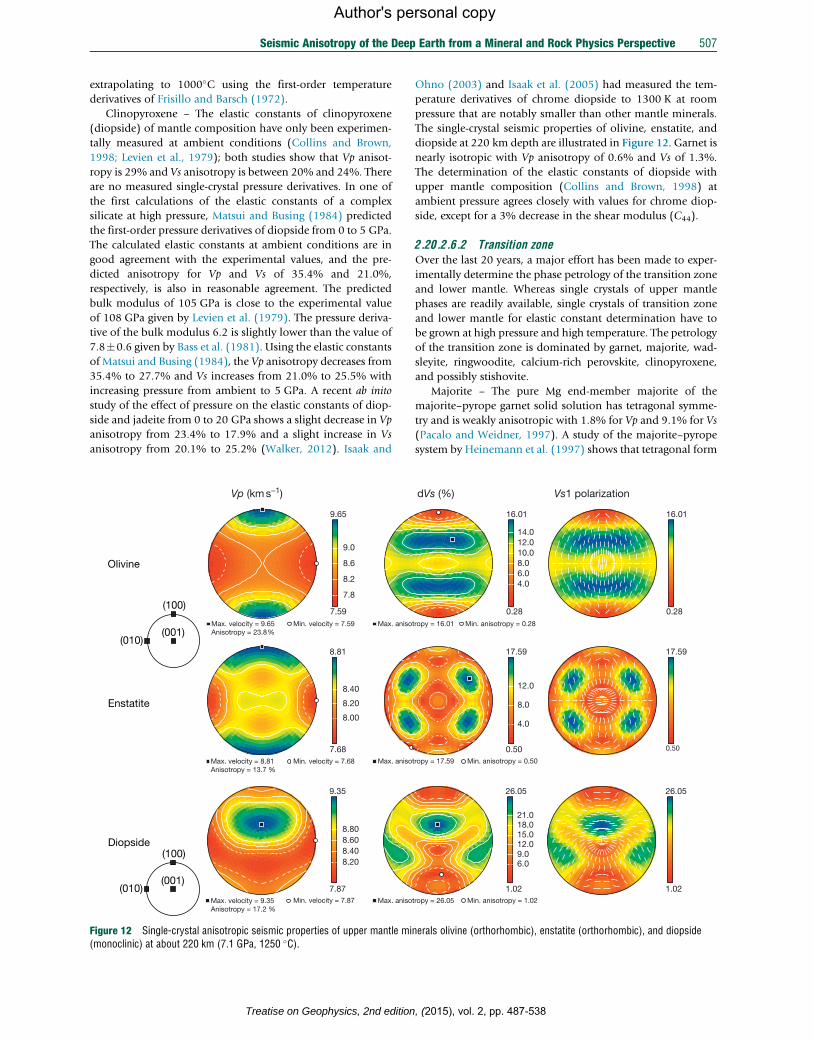
Seismic Anisotropy of the Deep Earth from a Mineral and Rock Physics Perspective 507
Author's personal copy
extrapolating to 1000�C using the first-order temperature
derivatives of Frisillo and Barsch (1972).
Clinopyroxene – The elastic constants of clinopyroxene
(diopside) of mantle composition have only been experimen-
tally measured at ambient conditions (Collins and Brown,
1998; Levien et al., 1979); both studies show that Vp anisot-
ropy is 29% and Vs anisotropy is between 20% and 24%. There
are no measured single-crystal pressure derivatives. In one of
the first calculations of the elastic constants of a complex
silicate at high pressure, Matsui and Busing (1984) predicted
the first-order pressure derivatives of diopside from 0 to 5 GPa.
The calculated elastic constants at ambient conditions are in
good agreement with the experimental values, and the pre-
dicted anisotropy for Vp and Vs of 35.4% and 21.0%,
respectively, is also in reasonable agreement. The predicted
bulk modulus of 105 GPa is close to the experimental value
of 108 GPa given by Levien et al. (1979). The pressure deriva-
tive of the bulk modulus 6.2 is slightly lower than the value of
7.8�0.6 given by Bass et al. (1981). Using the elastic constants
of Matsui and Busing (1984), the Vp anisotropy decreases from
35.4% to 27.7% and Vs increases from 21.0% to 25.5% with
increasing pressure from ambient to 5 GPa. A recent ab inito
study of the effect of pressure on the elastic constants of diop-
side and jadeite from 0 to 20 GPa shows a slight decrease in Vp
anisotropy from 23.4% to 17.9% and a slight increase in Vs
anisotropy from 20.1% to 25.2% (Walker, 2012). Isaak and
9.35
7.87
8.20 8.40 8.60 8.80
Diopside
9.65
7.59 Max. velocity = 9.65Anisotropy = 23.8%
Max. velocity = 8.81Anisotropy = 13.7 %
Max. velocity = 9.35Anisotropy = 17.2 %
Min. velocity = 7.59
Min. velocity = 7.68
Min. velocity = 7.87
7.8
8.2
8.6
9.0
Max. aniso
Max. aniso
Max. aniso
Olivine
8.81
7.68
8.00
8.20
8.40
Enstatite
(100)
(010)(001)
(100)
(010)(001)
Vp (km s−1)
Figure 12 Single-crystal anisotropic seismic properties of upper mantle mi(monoclinic) at about 220 km (7.1 GPa, 1250 �C).
Treatise on Geophysics, 2nd edition
Ohno (2003) and Isaak et al. (2005) had measured the tem-
perature derivatives of chrome diopside to 1300 K at room
pressure that are notably smaller than other mantle minerals.
The single-crystal seismic properties of olivine, enstatite, and
diopside at 220 km depth are illustrated in Figure 12. Garnet is
nearly isotropic with Vp anisotropy of 0.6% and Vs of 1.3%.
The determination of the elastic constants of diopside with
upper mantle composition (Collins and Brown, 1998) at
ambient pressure agrees closely with values for chrome diop-
side, except for a 3% decrease in the shear modulus (C44).
2.20.2.6.2 Transition zoneOver the last 20 years, a major effort has been made to exper-
imentally determine the phase petrology of the transition zone
and lower mantle. Whereas single crystals of upper mantle
phases are readily available, single crystals of transition zone
and lower mantle for elastic constant determination have to
be grown at high pressure and high temperature. The petrology
of the transition zone is dominated by garnet, majorite, wad-
sleyite, ringwoodite, calcium-rich perovskite, clinopyroxene,
and possibly stishovite.
Majorite – The pure Mg end-member majorite of the
majorite–pyrope garnet solid solution has tetragonal symme-
try and is weakly anisotropic with 1.8% for Vp and 9.1% for Vs
(Pacalo and Weidner, 1997). A study of the majorite–pyrope
system by Heinemann et al. (1997) shows that tetragonal form
26.05
1.02
6.0 9.0 12.0 15.0 18.0 21.0
26.05
1.02
16.01
0.28 tropy = 16.01
tropy = 17.59
tropy = 26.05
Min. anisotropy = 0.28
Min. anisotropy = 0.50
Min. anisotropy = 1.02
4.0 6.0 8.0 10.0 12.0 14.0
16.01
0.28
17.59
0.50
4.0
8.0
12.0
17.59
0.50
dVs (%) Vs1 polarization
nerals olivine (orthorhombic), enstatite (orthorhombic), and diopside
, (2015), vol. 2, pp. 487-538
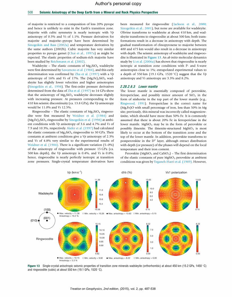
508 Seismic Anisotropy of the Deep Earth from a Mineral and Rock Physics Perspective
Author's personal copy
of majorite is restricted to a composition of less 20% pyrope
and hence is unlikely to exist in the Earth’s transition zone.
Majorite with cubic symmetry is nearly isotropic with Vp
anisotropy of 0.5% and Vs of 1.1%. Pressure derivatives for
majorite and majorite–pyrope have been determined by
Sinogeikin and Bass (2002a) and temperature derivatives by
the same authors (2002b). Cubic majorite has very similar
properties to pyrope garnet (Chai et al., 1997a) as might be
expected. The elastic properties of sodium-rich majorite have
been studied by Reichmann et al. (2002).
Wadsleyite – The elastic constants of Mg2SiO4 wadsleyite
were first determined by Sawamoto et al. (1984), and this early
determination was confirmed by Zha et al. (1997) with a Vp
anisotropy of 16% and Vs of 17%. The (Mg,Fe)2SiO4 wad-
sleyite has slightly lower velocities and higher anisotropies
(Sinogeikin et al., 1998). The first-order pressure derivatives
determined from the data of Zha et al. (1997) to 14 GPa show
that the anisotropy of Mg2SiO4 wadsleyite decreases slightly
with increasing pressure. At pressures corresponding to the
410 km seismic discontinuity (ca. 13.8 GPa), the Vp anisotropy
would be 11.0% and Vs 12.5%.
Ringwoodite – The elastic constants of Mg2SiO4 ringwoo-
dite were first measured by Weidner et al. (1984) and
(Mg,Fe)2SiO4 ringwoodite by Sinogeikin et al. (1998) at ambi-
ent conditions with Vp anisotropy of 3.6 and 4.7% and Vs of
7.9 and 10.3%, respectively. Kiefer et al. (1997) had calculated
the elastic constants of Mg2SiO4 ringwoodite to 30 GPa. Their
constants at ambient conditions give a Vp anisotropy of 2.3%
and Vs of 4.8% very similar to the experimental results of
Weidner et al. (1984). There is a significant variation (5–0%)
of the anisotropy of ringwoodite with pressure 15 GPa (ca.
500 km depth), the Vp anisotropy is 0.4%, and Vs is 0.8%;
hence, ringwoodite is nearly perfectly isotropic at transition
zone pressures. Single-crystal temperature derivatives have
10.15
9.82
9.90
9.95
10.00
10.05
10.10
Ringwoodite
11.36
10.26
10.4
10.6
10.8
11.0
Wadsleyite
(100)
(010)(001)
Vp (km s−1)
Max. velocity = 11.36Anisotropy = 10.2 %
Min. velocity = 10.26 Max. anisotr
Max. velocity = 10.15Anisotropy = 3.3 %
Min. velocity = 9.82 Max. anisot
Figure 13 Single-crystal anisotropic seismic properties of transition zone mand ringwoodite (cubic) at about 550 km (19.1 GPa, 1520 �C).
Treatise on Geophysics, 2nd edition,
been measured for ringwoodite ( Jackson et al., 2000;
Sinogeikin et al., 2001), but none are available for wadsleyite.
Olivine transforms to wadsleyite at about 410 km, and wad-
sleyite transforms to ringwoodite at about 500 km; both trans-
formations result in a decrease in anisotropy with depth. The
gradual transformation of clinopyroxene to majorite between
400 and 475 km would also result in a decrease in anisotropy
with depth. The seismic anisotropy of wadsleyite and ringwoo-
dite is illustrated in Figure 13. An ab initiomolecular dynamics
study by Li et al. (2006a) has shown that ringwoodite is nearly
isotropic at transition zone conditions with P- and S-wave
anisotropies close to 1%; extrapolated experimental values to
a depth of 550 km (19.1 GPa, 1520 �C) suggest that the Vp
anisotropy and Vs anisotropy are 3.3% and 8.2%.
2.20.2.6.3 Lower mantleThe lower mantle is essentially composed of perovskite,
ferropericlase, and possibly minor amount of SiO2 in the
form of stishovite in the top part of the lower mantle (e.g.,
Ringwood, 1991). Ferropericlase is the correct name for
(Mg,Fe)O with small percentage of iron, less than 50% in Mg
site; previously, this mineral was incorrectly called magnesiow-
ustite, which should have more than 50% Fe. It is commonly
assumed that there is about 20% Fe in ferropericlase in the
lower mantle. MgSiO3 may be in the form of perovskite or
possibly ilmenite. The ilmenite-structured MgSiO3 is most
likely to occur at the bottom of the transition zone and the
top of the lower mantle. In addition, perovskite transforms to
postperovskite in the D00 layer, although extract distribution
with depth (or pressure) of the phases will depend on the local
temperature and their iron content.
Perovskite (MgSiO3 and CaSiO3) – The first determination
of the elastic constants of pure MgSiO3 perovskite at ambient
conditions was given by Yeganeh-Haeri et al. (1989). However,
8.22
0.00
1.0
3.0
5.0
7.0
8.22
0.00
13.63
0.15
Min. anisotropy = 0.15
4.0
6.0
8.0
10.0
13.63
0.15
dVs (%) Vs1 polarization
opy = 13.63
Min. anisotropy = 0.00ropy = 8.22
inerals wadsleyite (orthorhombic) at about 450 km (15.2 GPa, 1450 �C)
(2015), vol. 2, pp. 487-538
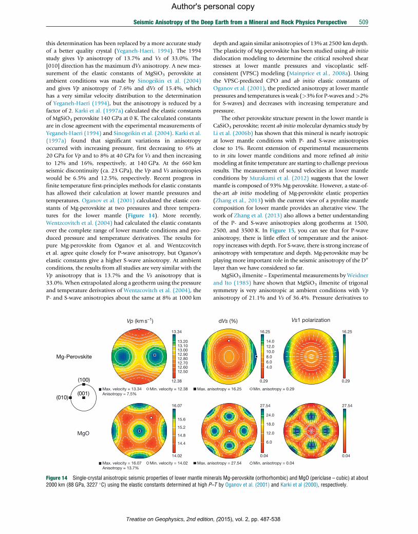
Seismic Anisotropy of the Deep Earth from a Mineral and Rock Physics Perspective 509
Author's personal copy
this determination has been replaced by a more accurate study
of a better quality crystal (Yeganeh-Haeri, 1994). The 1994
study gives Vp anisotropy of 13.7% and Vs of 33.0%. The
[010] direction has the maximum dVs anisotropy. A new mea-
surement of the elastic constants of MgSiO3 perovskite at
ambient conditions was made by Sinogeikin et al. (2004)
and gives Vp anisotropy of 7.6% and dVs of 15.4%, which
has a very similar velocity distribution to the determination
of Yeganeh-Haeri (1994), but the anisotropy is reduced by a
factor of 2. Karki et al. (1997a) calculated the elastic constants
of MgSiO3 perovskite 140 GPa at 0 K. The calculated constants
are in close agreement with the experimental measurements of
Yeganeh-Haeri (1994) and Sinogeikin et al. (2004). Karki et al.
(1997a) found that significant variations in anisotropy
occurred with increasing pressure, first decreasing to 6% at
20 GPa for Vp and to 8% at 40 GPa for Vs and then increasing
to 12% and 16%, respectively, at 140 GPa. At the 660 km
seismic discontinuity (ca. 23 GPa), the Vp and Vs anisotropies
would be 6.5% and 12.5%, respectively. Recent progress in
finite temperature first-principles methods for elastic constants
has allowed their calculation at lower mantle pressures and
temperatures. Oganov et al. (2001) calculated the elastic con-
stants of Mg-perovskite at two pressures and three tempera-
tures for the lower mantle (Figure 14). More recently,
Wentzcovitch et al. (2004) had calculated the elastic constants
over the complete range of lower mantle conditions and pro-
duced pressure and temperature derivatives. The results for
pure Mg-perovskite from Oganov et al. and Wentzcovitch
et al. agree quite closely for P-wave anisotropy, but Oganov’s
elastic constants give a higher S-wave anisotropy. At ambient
conditions, the results from all studies are very similar with the
Vp anisotropy that is 13.7% and the Vs anisotropy that is
33.0%.When extrapolated along a geotherm using the pressure
and temperature derivatives of Wentzcovitch et al. (2004), the
P- and S-wave anisotropies about the same at 8% at 1000 km
MgO
13.34
12.38
12.50 12.60 12.70 12.80 12.90 13.00 13.10 13.20
Mg-Perovskite
16.07
14.02
14.4
14.8
15.2
15.6
(100)
(010)(001)
Vp (km s−1)
Min. velocity = 12.38Max. velocity = 13.34Anisotropy = 7.5%
Max. an
Min. velocity = 14.02Max. velocity = 16.07Anisotropy = 13.7%
Max. an
Figure 14 Single-crystal anisotropic seismic properties of lower mantle min2000 km (88 GPa, 3227 �C) using the elastic constants determined at high P
Treatise on Geophysics, 2nd edition
depth and again similar anisotropies of 13% at 2500 km depth.
The plasticity of Mg-perovskite has been studied using ab initio
dislocation modeling to determine the critical resolved shear
stresses at lower mantle pressures and viscoplastic self-
consistent (VPSC) modeling (Mainprice et al., 2008a). Using
the VPSC-predicted CPO and ab initio elastic constants of
Oganov et al. (2001), the predicted anisotropy at lower mantle
pressures and temperatures is weak (>3% for P-waves and>2%
for S-waves) and decreases with increasing temperature and
pressure.
The other perovskite structure present in the lower mantle is
CaSiO3 perovskite; recent ab initiomolecular dynamics study by
Li et al. (2006b) has shown that this mineral is nearly isotropic
at lower mantle conditions with P- and S-wave anisotropies
close to 1%. Recent extension of experimental measurements
to in situ lower mantle conditions and more refined ab initio
modeling at finite temperature are starting to challenge previous
results. The measurement of sound velocities at lower mantle
conditions by Murakami et al. (2012) suggests that the lower
mantle is composed of 93%Mg-perovskite. However, a state-of-
the-art ab initio modeling of Mg-perovskite elastic properties
(Zhang et al., 2013) with the current view of a pyrolite mantle
composition for lower mantle provides an alterative view. The
work of Zhang et al. (2013) also allows a better understanding
of the P- and S-wave anisotropies along geotherms at 1500,
2500, and 3500 K. In Figure 15, you can see that for P-wave
anisotropy, there is little effect of temperature and the anisot-
ropy increases with depth. For S-wave, there is strong increase of
anisotropy with temperature and depth. Mg-perovskite may be
playing more important role in the seismic anisotropy of the D00
layer than we have considered so far.
MgSiO3 ilmenite – Experimental measurements byWeidner
and Ito (1985) have shown that MgSiO3 ilmenite of trigonal
symmetry is very anisotropic at ambient conditions with Vp
anisotropy of 21.1% and Vs of 36.4%. Pressure derivatives to
16.25
0.29
4.0 6.0 8.0 10.0 12.0 14.0
16.25
0.29
27.54
0.04
6.0
12.0
18.0
24.0
27.54
0.04
dVs (%) Vs1 polarization
Min. anisotropy = 0.29isotropy = 16.25
Min. anisotropy = 0.04isotropy = 27.54
erals Mg-perovskite (orthorhombic) and MgO (periclase – cubic) at about–T by Oganov et al. (2001) and Karki et al (2000), respectively.
, (2015), vol. 2, pp. 487-538
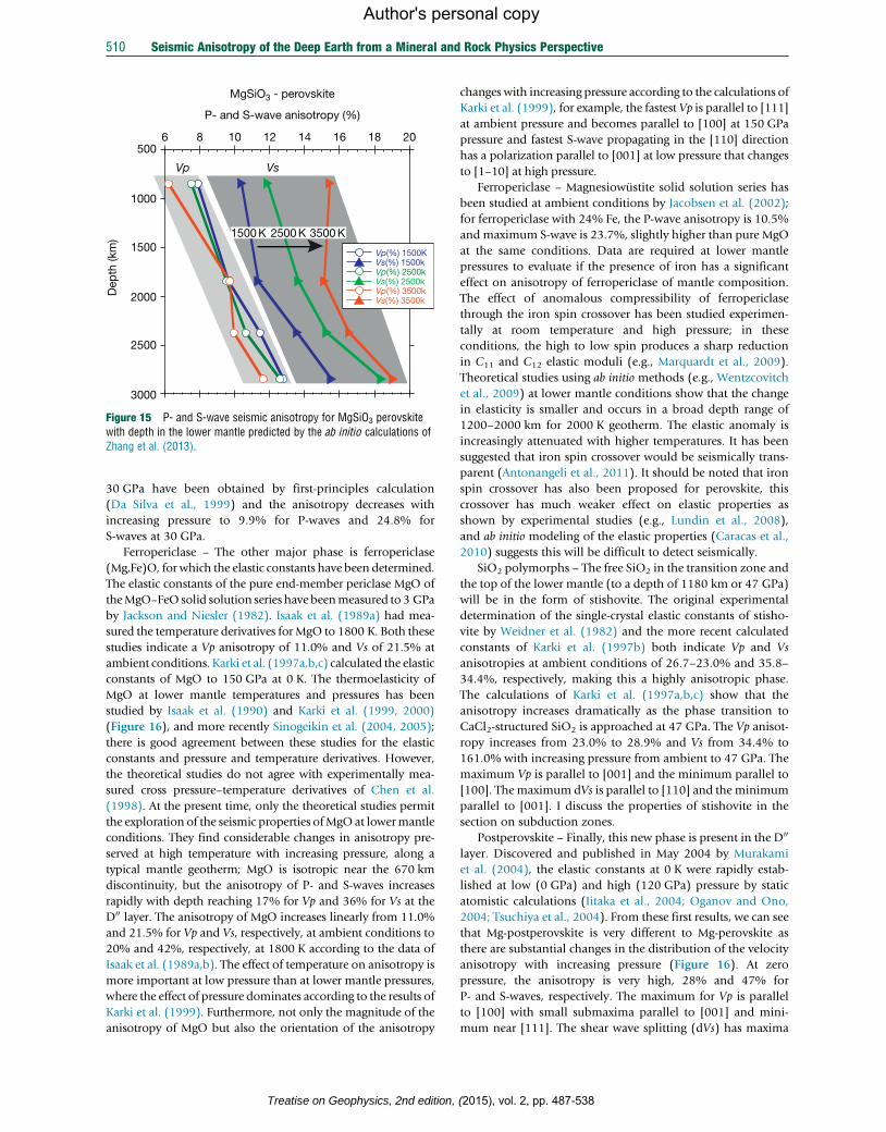
P- and S-wave anisotropy (%)D
epth
(km
)
6 8 10 12 14 16 18 20500
1000
1500
2000
2500
3000
Vp(%) 1500KVs(%) 1500kVp(%) 2500kVs(%) 2500kVp(%) 3500kVs(%) 3500k
VsVp
3500 K2500 K1500 K
MgSiO3 - perovskite
Figure 15 P- and S-wave seismic anisotropy for MgSiO3 perovskitewith depth in the lower mantle predicted by the ab initio calculations ofZhang et al. (2013).
510 Seismic Anisotropy of the Deep Earth from a Mineral and Rock Physics Perspective
Author's personal copy
30 GPa have been obtained by first-principles calculation
(Da Silva et al., 1999) and the anisotropy decreases with
increasing pressure to 9.9% for P-waves and 24.8% for
S-waves at 30 GPa.
Ferropericlase – The other major phase is ferropericlase
(Mg,Fe)O, for which the elastic constants have been determined.
The elastic constants of the pure end-member periclase MgO of
theMgO–FeO solid solution series have beenmeasured to 3 GPa
by Jackson and Niesler (1982). Isaak et al. (1989a) had mea-
sured the temperature derivatives for MgO to 1800 K. Both these
studies indicate a Vp anisotropy of 11.0% and Vs of 21.5% at
ambient conditions. Karki et al. (1997a,b,c) calculated the elastic
constants of MgO to 150 GPa at 0 K. The thermoelasticity of
MgO at lower mantle temperatures and pressures has been
studied by Isaak et al. (1990) and Karki et al. (1999, 2000)
(Figure 16), and more recently Sinogeikin et al. (2004, 2005);
there is good agreement between these studies for the elastic
constants and pressure and temperature derivatives. However,
the theoretical studies do not agree with experimentally mea-
sured cross pressure–temperature derivatives of Chen et al.
(1998). At the present time, only the theoretical studies permit
the exploration of the seismic properties ofMgOat lowermantle
conditions. They find considerable changes in anisotropy pre-
served at high temperature with increasing pressure, along a
typical mantle geotherm; MgO is isotropic near the 670 km
discontinuity, but the anisotropy of P- and S-waves increases
rapidly with depth reaching 17% for Vp and 36% for Vs at the
D00 layer. The anisotropy of MgO increases linearly from 11.0%
and 21.5% for Vp and Vs, respectively, at ambient conditions to
20% and 42%, respectively, at 1800 K according to the data of
Isaak et al. (1989a,b). The effect of temperature on anisotropy is
more important at low pressure than at lower mantle pressures,
where the effect of pressure dominates according to the results of
Karki et al. (1999). Furthermore, not only the magnitude of the
anisotropy of MgO but also the orientation of the anisotropy
Treatise on Geophysics, 2nd edition,
changes with increasing pressure according to the calculations of
Karki et al. (1999), for example, the fastest Vp is parallel to [111]
at ambient pressure and becomes parallel to [100] at 150 GPa
pressure and fastest S-wave propagating in the [110] direction
has a polarization parallel to [001] at low pressure that changes
to [1–10] at high pressure.
Ferropericlase – Magnesiowustite solid solution series has
been studied at ambient conditions by Jacobsen et al. (2002);
for ferropericlase with 24% Fe, the P-wave anisotropy is 10.5%
and maximum S-wave is 23.7%, slightly higher than pure MgO
at the same conditions. Data are required at lower mantle
pressures to evaluate if the presence of iron has a significant
effect on anisotropy of ferropericlase of mantle composition.
The effect of anomalous compressibility of ferropericlase
through the iron spin crossover has been studied experimen-
tally at room temperature and high pressure; in these
conditions, the high to low spin produces a sharp reduction
in C11 and C12 elastic moduli (e.g., Marquardt et al., 2009).
Theoretical studies using ab initio methods (e.g., Wentzcovitch
et al., 2009) at lower mantle conditions show that the change
in elasticity is smaller and occurs in a broad depth range of
1200–2000 km for 2000 K geotherm. The elastic anomaly is
increasingly attenuated with higher temperatures. It has been
suggested that iron spin crossover would be seismically trans-
parent (Antonangeli et al., 2011). It should be noted that iron
spin crossover has also been proposed for perovskite, this
crossover has much weaker effect on elastic properties as
shown by experimental studies (e.g., Lundin et al., 2008),
and ab initio modeling of the elastic properties (Caracas et al.,
2010) suggests this will be difficult to detect seismically.
SiO2 polymorphs – The free SiO2 in the transition zone and
the top of the lower mantle (to a depth of 1180 km or 47 GPa)
will be in the form of stishovite. The original experimental
determination of the single-crystal elastic constants of stisho-
vite by Weidner et al. (1982) and the more recent calculated
constants of Karki et al. (1997b) both indicate Vp and Vs
anisotropies at ambient conditions of 26.7–23.0% and 35.8–
34.4%, respectively, making this a highly anisotropic phase.
The calculations of Karki et al. (1997a,b,c) show that the
anisotropy increases dramatically as the phase transition to
CaCl2-structured SiO2 is approached at 47 GPa. The Vp anisot-
ropy increases from 23.0% to 28.9% and Vs from 34.4% to
161.0% with increasing pressure from ambient to 47 GPa. The
maximum Vp is parallel to [001] and the minimum parallel to
[100]. Themaximum dVs is parallel to [110] and the minimum
parallel to [001]. I discuss the properties of stishovite in the
section on subduction zones.
Postperovskite – Finally, this new phase is present in the D00
layer. Discovered and published in May 2004 by Murakami
et al. (2004), the elastic constants at 0 K were rapidly estab-
lished at low (0 GPa) and high (120 GPa) pressure by static
atomistic calculations (Iitaka et al., 2004; Oganov and Ono,
2004; Tsuchiya et al., 2004). From these first results, we can see
that Mg-postperovskite is very different to Mg-perovskite as
there are substantial changes in the distribution of the velocity
anisotropy with increasing pressure (Figure 16). At zero
pressure, the anisotropy is very high, 28% and 47% for
P- and S-waves, respectively. The maximum for Vp is parallel
to [100] with small submaxima parallel to [001] and mini-
mum near [111]. The shear wave splitting (dVs) has maxima
(2015), vol. 2, pp. 487-538
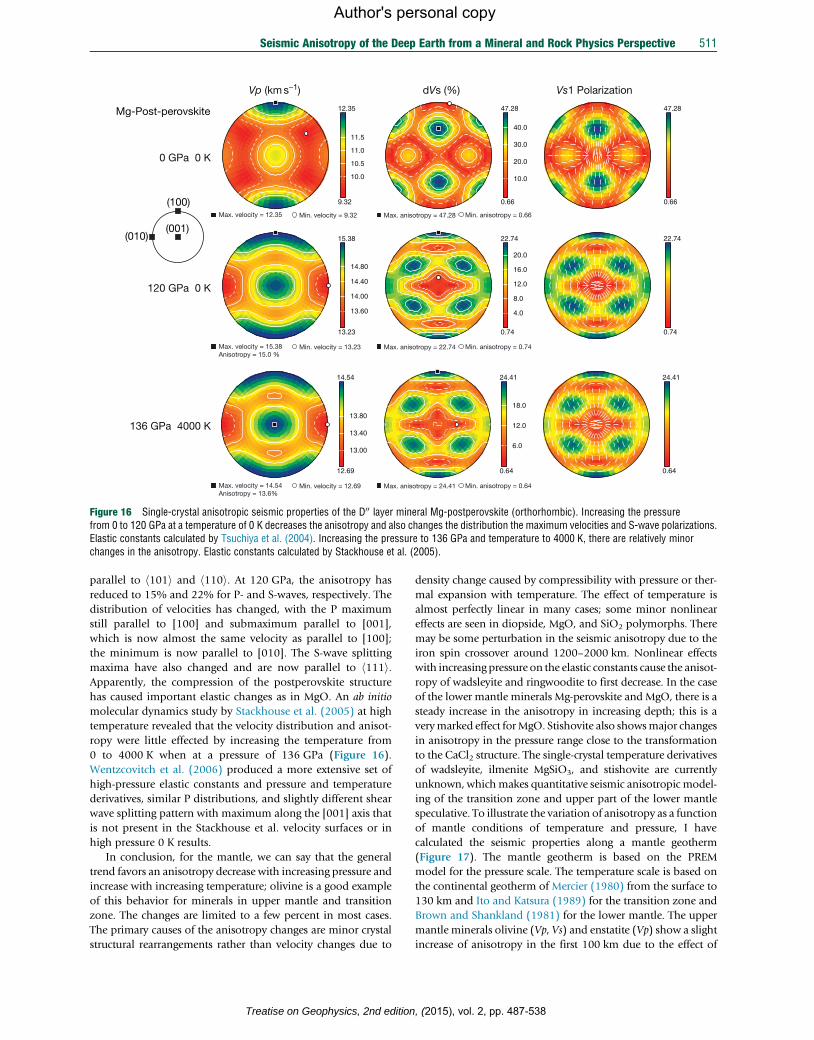
12.35
9.32
10.0
10.5
11.0
11.5
47.28
0.66
10.0
20.0
30.0
40.0
47.28
0.66
15.38
13.23
13.60
14.00
14.40
14.80
22.74
0.74
4.0
8.0
12.0
16.0
20.0
22.74
0.74
14.54
12.69
13.00
13.40
13.80
24.41
0.64
6.0
12.0
18.0
24.41
0.64
0 GPa 0 K
120 GPa 0 K
136 GPa 4000 K
(100)
(010)(001)
Vp (km s−1) dVs (%) Vs1 Polarization
Mg-Post-perovskite
Min. anisotropy = 0.64Max. velocity = 14.54Anisotropy = 13.6%
Min. velocity = 12.69 Max. anisotropy = 24.41
Min. anisotropy = 0.66Max. velocity = 12.35 Min. velocity = 9.32 Max. anisotropy = 47.28
Min. anisotropy = 0.74Max. velocity = 15.38Anisotropy = 15.0 %
Min. velocity = 13.23 Max. anisotropy = 22.74
Figure 16 Single-crystal anisotropic seismic properties of the D00 layer mineral Mg-postperovskite (orthorhombic). Increasing the pressurefrom 0 to 120 GPa at a temperature of 0 K decreases the anisotropy and also changes the distribution the maximum velocities and S-wave polarizations.Elastic constants calculated by Tsuchiya et al. (2004). Increasing the pressure to 136 GPa and temperature to 4000 K, there are relatively minorchanges in the anisotropy. Elastic constants calculated by Stackhouse et al. (2005).
Seismic Anisotropy of the Deep Earth from a Mineral and Rock Physics Perspective 511
Author's personal copy
parallel to h101i and h110i. At 120 GPa, the anisotropy has
reduced to 15% and 22% for P- and S-waves, respectively. The
distribution of velocities has changed, with the P maximum
still parallel to [100] and submaximum parallel to [001],
which is now almost the same velocity as parallel to [100];
the minimum is now parallel to [010]. The S-wave splitting
maxima have also changed and are now parallel to h111i.Apparently, the compression of the postperovskite structure
has caused important elastic changes as in MgO. An ab initio
molecular dynamics study by Stackhouse et al. (2005) at high
temperature revealed that the velocity distribution and anisot-
ropy were little effected by increasing the temperature from
0 to 4000 K when at a pressure of 136 GPa (Figure 16).
Wentzcovitch et al. (2006) produced a more extensive set of
high-pressure elastic constants and pressure and temperature
derivatives, similar P distributions, and slightly different shear
wave splitting pattern with maximum along the [001] axis that
is not present in the Stackhouse et al. velocity surfaces or in
high pressure 0 K results.
In conclusion, for the mantle, we can say that the general
trend favors an anisotropy decrease with increasing pressure and
increase with increasing temperature; olivine is a good example
of this behavior for minerals in upper mantle and transition
zone. The changes are limited to a few percent in most cases.
The primary causes of the anisotropy changes are minor crystal
structural rearrangements rather than velocity changes due to
Treatise on Geophysics, 2nd edition
density change caused by compressibility with pressure or ther-
mal expansion with temperature. The effect of temperature is
almost perfectly linear in many cases; some minor nonlinear
effects are seen in diopside, MgO, and SiO2 polymorphs. There
may be some perturbation in the seismic anisotropy due to the
iron spin crossover around 1200–2000 km. Nonlinear effects
with increasing pressure on the elastic constants cause the anisot-
ropy of wadsleyite and ringwoodite to first decrease. In the case
of the lower mantle minerals Mg-perovskite and MgO, there is a
steady increase in the anisotropy in increasing depth; this is a
verymarked effect forMgO. Stishovite also showsmajor changes
in anisotropy in the pressure range close to the transformation
to the CaCl2 structure. The single-crystal temperature derivatives
of wadsleyite, ilmenite MgSiO3, and stishovite are currently
unknown, whichmakes quantitative seismic anisotropic model-
ing of the transition zone and upper part of the lower mantle
speculative. To illustrate the variation of anisotropy as a function
of mantle conditions of temperature and pressure, I have
calculated the seismic properties along a mantle geotherm
(Figure 17). The mantle geotherm is based on the PREM
model for the pressure scale. The temperature scale is based on
the continental geotherm of Mercier (1980) from the surface to
130 km and Ito and Katsura (1989) for the transition zone and
Brown and Shankland (1981) for the lower mantle. The upper
mantle minerals olivine (Vp, Vs) and enstatite (Vp) show a slight
increase of anisotropy in the first 100 km due to the effect of
, (2015), vol. 2, pp. 487-538
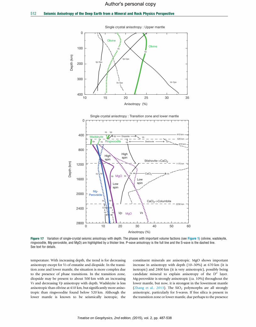
10 15 20 25 30 35
0
100
200
300
400
Single crystal anisotropy : Upper mantle
Anisotropy (%)
Dep
th (k
m)
Vs Cpx
Vp Cpx
Vp
Vs Opx
Vp Opx
0 10 20 30 40 50 60
0
400
800
1200
1600
2000
2400
2800
Single crystal anisotropy : Transition zone and lower mantle
Anisotropy (%)
Dep
th (k
m)
VpVs
670 km
Vs
Vs
Vp CaCl2
1170 kmStishovite->CaCl2
DiopsideVp520 km
Stishovite
Vp Vs
Colum bite
CaCl2->Columbite2230 km
410 km
VpVs
Vp Vs
Vp Vs
MgO
VsVp
Vp Vs
VpVs
Mg-Perovskite
MgO
Wadsleyite
Ringwoodite
Olivine
Olivine
Vs
Lowspin
Highspin
Highspin
Lowspin
Figure 17 Variation of single-crystal seismic anisotropy with depth. The phases with important volume factions (see Figure 1) (olivine, wadsleyite,ringwoodite, Mg-perovskite, and MgO) are highlighted by a thicker line. P-wave anisotropy is the full line and the S-wave is the dashed line.See text for details.
512 Seismic Anisotropy of the Deep Earth from a Mineral and Rock Physics Perspective
Author's personal copy
temperature. With increasing depth, the trend is for decreasing
anisotropy except for Vs of enstatite and diopside. In the transi-
tion zone and lower mantle, the situation is more complex due
to the presence of phase transitions. In the transition zone,
diopside may be present to about 500 km with an increasing
Vs and decreasing Vp anisotropy with depth. Wadsleyite is less
anisotropic than olivine at 410 km, but significantlymore aniso-
tropic than ringwoodite found below 520 km. Although the
lower mantle is known to be seismically isotropic, the
Treatise on Geophysics, 2nd edition,
constituent minerals are anisotropic. MgO shows important
increase in anisotropy with depth (10–30%) at 670 km (it is
isotropic) and 2800 km (it is very anisotropic), possibly being
candidate mineral to explain anisotropy of the D00 layer.
Mg-perovskite is strongly anisotropic (ca. 10%) throughout the
lower mantle, but now, it is strongest in the lowermost mantle
(Zhang et al., 2013). The SiO2 polymorphs are all strongly
anisotropic, particularly for S-waves. If free silica is present in
the transition zone or lowermantle, due perhaps to the presence
(2015), vol. 2, pp. 487-538
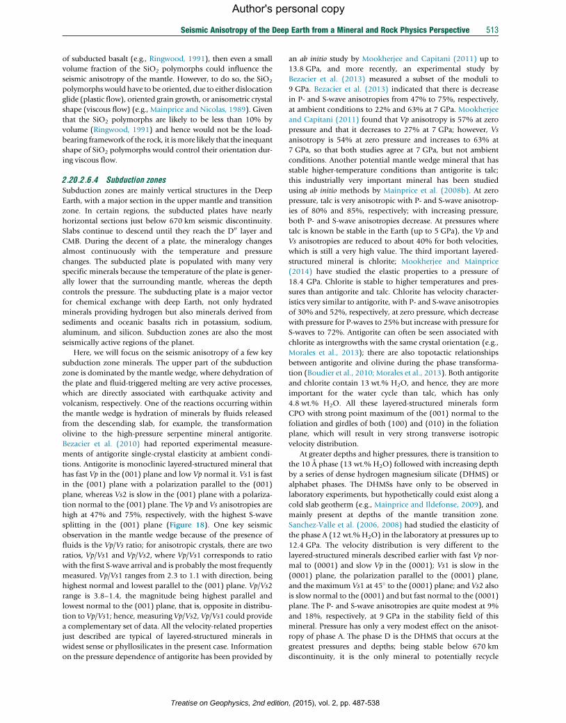
Seismic Anisotropy of the Deep Earth from a Mineral and Rock Physics Perspective 513
Author's personal copy
of subducted basalt (e.g., Ringwood, 1991), then even a small
volume fraction of the SiO2 polymorphs could influence the
seismic anisotropy of the mantle. However, to do so, the SiO2
polymorphswould have to be oriented, due to either dislocation
glide (plastic flow), oriented grain growth, or anisometric crystal
shape (viscous flow) (e.g., Mainprice and Nicolas, 1989). Given
that the SiO2 polymorphs are likely to be less than 10% by
volume (Ringwood, 1991) and hence would not be the load-
bearing framework of the rock, it ismore likely that the inequant
shape of SiO2 polymorphs would control their orientation dur-
ing viscous flow.
2.20.2.6.4 Subduction zonesSubduction zones are mainly vertical structures in the Deep
Earth, with a major section in the upper mantle and transition
zone. In certain regions, the subducted plates have nearly
horizontal sections just below 670 km seismic discontinuity.
Slabs continue to descend until they reach the D00 layer andCMB. During the decent of a plate, the mineralogy changes
almost continuously with the temperature and pressure
changes. The subducted plate is populated with many very
specific minerals because the temperature of the plate is gener-
ally lower that the surrounding mantle, whereas the depth
controls the pressure. The subducting plate is a major vector
for chemical exchange with deep Earth, not only hydrated
minerals providing hydrogen but also minerals derived from
sediments and oceanic basalts rich in potassium, sodium,
aluminum, and silicon. Subduction zones are also the most
seismically active regions of the planet.
Here, we will focus on the seismic anisotropy of a few key
subduction zone minerals. The upper part of the subduction
zone is dominated by the mantle wedge, where dehydration of
the plate and fluid-triggered melting are very active processes,
which are directly associated with earthquake activity and
volcanism, respectively. One of the reactions occurring within
the mantle wedge is hydration of minerals by fluids released
from the descending slab, for example, the transformation
olivine to the high-pressure serpentine mineral antigorite.
Bezacier et al. (2010) had reported experimental measure-
ments of antigorite single-crystal elasticity at ambient condi-
tions. Antigorite is monoclinic layered-structured mineral that
has fast Vp in the (001) plane and low Vp normal it. Vs1 is fast
in the (001) plane with a polarization parallel to the (001)
plane, whereas Vs2 is slow in the (001) plane with a polariza-
tion normal to the (001) plane. The Vp and Vs anisotropies are
high at 47% and 75%, respectively, with the highest S-wave
splitting in the (001) plane (Figure 18). One key seismic
observation in the mantle wedge because of the presence of
fluids is the Vp/Vs ratio; for anisotropic crystals, there are two
ratios, Vp/Vs1 and Vp/Vs2, where Vp/Vs1 corresponds to ratio
with the first S-wave arrival and is probably themost frequently
measured. Vp/Vs1 ranges from 2.3 to 1.1 with direction, being
highest normal and lowest parallel to the (001) plane. Vp/Vs2
range is 3.8–1.4, the magnitude being highest parallel and
lowest normal to the (001) plane, that is, opposite in distribu-
tion to Vp/Vs1; hence, measuring Vp/Vs2, Vp/Vs1 could provide
a complementary set of data. All the velocity-related properties
just described are typical of layered-structured minerals in
widest sense or phyllosilicates in the present case. Information
on the pressure dependence of antigorite has been provided by
Treatise on Geophysics, 2nd edition
an ab initio study by Mookherjee and Capitani (2011) up to
13.8 GPa, and more recently, an experimental study by
Bezacier et al. (2013) measured a subset of the moduli to
9 GPa. Bezacier et al. (2013) indicated that there is decrease
in P- and S-wave anisotropies from 47% to 75%, respectively,
at ambient conditions to 22% and 63% at 7 GPa. Mookherjee
and Capitani (2011) found that Vp anisotropy is 57% at zero
pressure and that it decreases to 27% at 7 GPa; however, Vs
anisotropy is 54% at zero pressure and increases to 63% at
7 GPa, so that both studies agree at 7 GPa, but not ambient
conditions. Another potential mantle wedge mineral that has
stable higher-temperature conditions than antigorite is talc;
this industrially very important mineral has been studied
using ab initio methods by Mainprice et al. (2008b). At zero
pressure, talc is very anisotropic with P- and S-wave anisotrop-
ies of 80% and 85%, respectively; with increasing pressure,
both P- and S-wave anisotropies decrease. At pressures where
talc is known be stable in the Earth (up to 5 GPa), the Vp and
Vs anisotropies are reduced to about 40% for both velocities,
which is still a very high value. The third important layered-
structured mineral is chlorite; Mookherjee and Mainprice
(2014) have studied the elastic properties to a pressure of
18.4 GPa. Chlorite is stable to higher temperatures and pres-
sures than antigorite and talc. Chlorite has velocity character-
istics very similar to antigorite, with P- and S-wave anisotropies
of 30% and 52%, respectively, at zero pressure, which decrease
with pressure for P-waves to 25% but increase with pressure for
S-waves to 72%. Antigorite can often be seen associated with
chlorite as intergrowths with the same crystal orientation (e.g.,
Morales et al., 2013); there are also topotactic relationships
between antigorite and olivine during the phase transforma-
tion (Boudier et al., 2010; Morales et al., 2013). Both antigorite
and chlorite contain 13 wt.% H2O, and hence, they are more
important for the water cycle than talc, which has only
4.8 wt.% H2O. All these layered-structured minerals form
CPO with strong point maximum of the (001) normal to the
foliation and girdles of both (100) and (010) in the foliation
plane, which will result in very strong transverse isotropic
velocity distribution.
At greater depths and higher pressures, there is transition to
the 10 A phase (13 wt.% H2O) followed with increasing depth
by a series of dense hydrogen magnesium silicate (DHMS) or
alphabet phases. The DHMSs have only to be observed in
laboratory experiments, but hypothetically could exist along a
cold slab geotherm (e.g., Mainprice and Ildefonse, 2009), and
mainly present at depths of the mantle transition zone.
Sanchez-Valle et al. (2006, 2008) had studied the elasticity of
the phase A (12 wt.% H2O) in the laboratory at pressures up to
12.4 GPa. The velocity distribution is very different to the
layered-structured minerals described earlier with fast Vp nor-
mal to (0001) and slow Vp in the (0001); Vs1 is slow in the
(0001) plane, the polarization parallel to the (0001) plane,
and the maximum Vs1 at 45� to the (0001) plane; and Vs2 also
is slow normal to the (0001) and but fast normal to the (0001)
plane. The P- and S-wave anisotropies are quite modest at 9%
and 18%, respectively, at 9 GPa in the stability field of this
mineral. Pressure has only a very modest effect on the anisot-
ropy of phase A. The phase D is the DHMS that occurs at the
greatest pressures and depths; being stable below 670 km
discontinuity, it is the only mineral to potentially recycle
, (2015), vol. 2, pp. 487-538
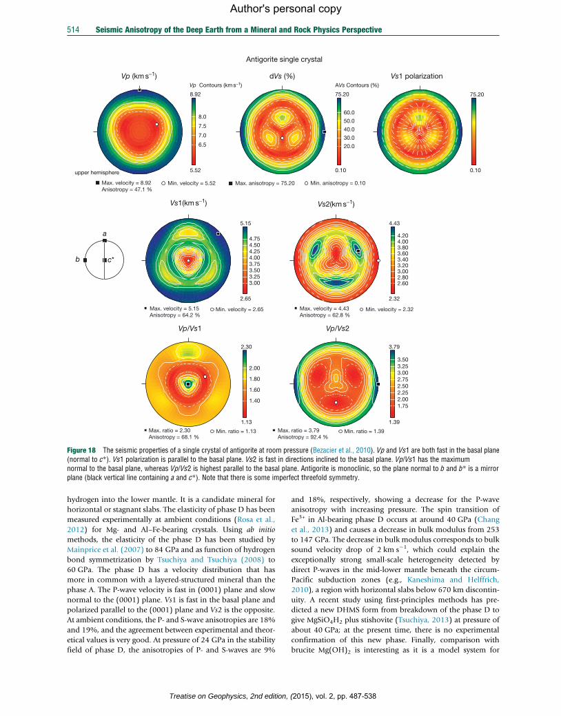
upper hemisphere
8.92
5.52
Vp Contours (km s−1)
6.5
7.0
7.5
8.0
75.20
0.10
AVs Contours (%)
20.0
30.0
40.0
50.0
60.0
75.20
0.10
2.30
1.13
1.40
1.60
1.80
2.00
3.79
1.39
1.75 2.00 2.25 2.50 2.75 3.00 3.25 3.50
b c*
a
Antigorite single crystal
Vp (km s−1) dVs (%) Vs1 polarization
Vp/Vs1 Vp/Vs2
5.15
2.65
3.00 3.25 3.50 3.75 4.00 4.25 4.50 4.75
4.43
2.32
2.60 2.80 3.00 3.20 3.40 3.60 3.80 4.00 4.20
Vs1(km s−1) Vs2(km s−1)
Min. anisotropy = 0.10Max. velocity = 8.92Anisotropy = 47.1 %
Min. velocity = 5.52 Max. anisotropy = 75.20
Max. velocity = 5.15Anisotropy = 64.2 %
Min. velocity = 2.65
Max. ratio = 2.30Anisotropy = 68.1 %
Min. ratio = 1.13 Max. ratio = 3.79Anisotropy = 92.4 %
Min. ratio = 1.39
Max. velocity = 4.43Anisotropy = 62.8 %
Min. velocity = 2.32
Figure 18 The seismic properties of a single crystal of antigorite at room pressure (Bezacier et al., 2010). Vp and Vs1 are both fast in the basal plane(normal to c*). Vs1 polarization is parallel to the basal plane. Vs2 is fast in directions inclined to the basal plane. Vp/Vs1 has the maximumnormal to the basal plane, whereas Vp/Vs2 is highest parallel to the basal plane. Antigorite is monoclinic, so the plane normal to b and b* is a mirrorplane (black vertical line containing a and c*). Note that there is some imperfect threefold symmetry.
514 Seismic Anisotropy of the Deep Earth from a Mineral and Rock Physics Perspective
Author's personal copy
hydrogen into the lower mantle. It is a candidate mineral for
horizontal or stagnant slabs. The elasticity of phase D has been
measured experimentally at ambient conditions (Rosa et al.,
2012) for Mg- and Al–Fe-bearing crystals. Using ab initio
methods, the elasticity of the phase D has been studied by
Mainprice et al. (2007) to 84 GPa and as function of hydrogen
bond symmetrization by Tsuchiya and Tsuchiya (2008) to
60 GPa. The phase D has a velocity distribution that has
more in common with a layered-structured mineral than the
phase A. The P-wave velocity is fast in (0001) plane and slow
normal to the (0001) plane. Vs1 is fast in the basal plane and
polarized parallel to the (0001) plane and Vs2 is the opposite.
At ambient conditions, the P- and S-wave anisotropies are 18%
and 19%, and the agreement between experimental and theor-
etical values is very good. At pressure of 24 GPa in the stability
field of phase D, the anisotropies of P- and S-waves are 9%
Treatise on Geophysics, 2nd edition,
and 18%, respectively, showing a decrease for the P-wave
anisotropy with increasing pressure. The spin transition of
Fe3+ in Al-bearing phase D occurs at around 40 GPa (Chang
et al., 2013) and causes a decrease in bulk modulus from 253
to 147 GPa. The decrease in bulk modulus corresponds to bulk
sound velocity drop of 2 km s�1, which could explain the
exceptionally strong small-scale heterogeneity detected by
direct P-waves in the mid-lower mantle beneath the circum-
Pacific subduction zones (e.g., Kaneshima and Helffrich,
2010), a region with horizontal slabs below 670 km discontin-
uity. A recent study using first-principles methods has pre-
dicted a new DHMS form from breakdown of the phase D to
give MgSiO4H2 plus stishovite (Tsuchiya, 2013) at pressure of
about 40 GPa; at the present time, there is no experimental
confirmation of this new phase. Finally, comparison with
brucite Mg(OH)2 is interesting as it is a model system for
(2015), vol. 2, pp. 487-538
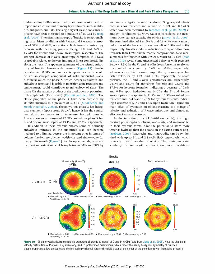
Seismic Anisotropy of the Deep Earth from a Mineral and Rock Physics Perspective 515
Author's personal copy
understanding DHMS under hydrostatic compression and an
important structural unit of many layer silicates, such as chlo-
rite, antigorite, and talc. The single-crystal elastic constants of
brucite have been measured to a pressure of 15 GPa by Jiang
et al. (2006). The seismic anisotropy of brucite is exceptionally
high at ambient conditions with P-wave and S-wave anisotrop-
ies of 57% and 46%, respectively. Both forms of anisotropy
decrease with increasing pressure being 12% and 24% at
15 GPa for P-wave and S-wave anisotropies, respectively. The
stronger decrease of P-wave anisotropy compared to S-wave
is probably related to the very important linear compressibility
along the c-axis. The apparent symmetry of the seismic anisot-
ropy of brucite changes with pressure (Figure 19). Brucite
is stable to 80 GPa and modest temperatures, so it could
be an anisotropic component of cold subducted slabs.
A mineral called the phase X, which occurs as hydrous and
anhydrous forms and is stable at transition zone pressures and
temperatures, could contribute to mineralogy of slabs. The
phase X is the reaction product of the breakdown of potassium
rich amphibole (K-richterite) (Konzett and Fei, 2000). The
elastic properties of the phase X have been predicted by
ab initio methods to a pressure of 30 GPa (Mookherjee and
Steinle-Neumann, 2009a). The anhydrous phase X has hexag-
onal symmetry (space group P63cm); hence, it has the equiva-
lent elastic symmetry to a transverse isotropic sample.
At transition zone pressure of 22 GPa, anhydrous phase X has
P- and S-wave anisotropies of 13.1% and 12.2%, respectively.
In addition to these hydrous phases, some of normally
anhydrous minerals in the subducted slab can become
hydrated to a limited degree; the important ones in terms of
volume fraction are olivine, wadsleyite, and ringwoodite for
the pyrolite mantle (Figure 1). For the upper mantle, olivine is
the most important mineral being between 50% and 70% by
Upper hemisphere
8.17
4.56
5.5
6.0
6.5
7.0
7.5
(0110)
(2110)P velocity (km s−1)
9.31
8.25
8.40
8.60
8.80
9.00
9.20
P = 0 GPa
P = 14.6 GPa
Max. velocity = 8.17Anisotropy = 56.7 %
Min. velocity = 4.56 Max. anisot
Max. velocity = 9.31Anisotropy = 12.1 %
Min. velocity = 8.25 Max. anisot
Figure 19 Single-crystal anisotropic seismic properties of brucite (trigonal)velocity distribution of P-waves, dVs anisotropy, and S1 polarization orientatielastic properties at low pressure and the increasingly trigonal nature (threef
Treatise on Geophysics, 2nd edition
volume of a typical mantle peridotite. Single-crystal elastic
constants for forsterite and olivine with 0.9 and 0.8 wt.%
water have been measured by Jacobsen et al. (2008, 2009) at
ambient conditions; 0.9 wt.% water is considered the maxi-
mum water storage capacity for olivine (Smyth et al., 2006).
The combined effect of 3 mol% Fe and 0.8 wt.% water causes a
reduction of the bulk and shear moduli of 2.9% and 4.5%,
respectively. Greater modulus reductions are expected for more
iron-rich than Fo90 olivine mantle compositions. New mea-
surements for forsterite with 0.9 wt.% water to 14 GPa (Mao
et al., 2010) reveal some unexpected behavior with pressure.
Below�3.5 GPa, the Vp and Vs of hydrous forsterite are slower
than anhydrous crystal by 0.6% and 0.4%, respectively,
whereas above this pressure range, the hydrous crystal has
faster velocities by 1.1% and 1.9%, respectively. At room
pressure, the P- and S-wave anisotropies are, respectively,
24.7% and 18.0% for anhydrous forsterite and 23.9% and
17.8% for hydrous forsterite, indicating a decrease of 0.8%
and 0.2% upon hydration. At 14 GPa, the P- and S-wave
anisotropies are, respectively, 21.2% and 13.5% for anhydrous
forsterite and 15.4% and 12.1% for hydrous forsterite, indicat-
ing a decrease of 6.0% and 1.4% upon hydration. Hence, the
main effect of hydration on olivine elasticity is a change of
velocity and reduction of P-wave anisotropy and almost no
effect on S-wave anisotropy.
In the transition zone (410–670 km depth), the high-
pressure polymorphs of olivine, wadsleyite, and ringwoodite,
in their hydrous forms, have the potential to store more
water as hydroxyl than the oceans on the Earth’s surface (e.g.,
Jacobsen, 2006). Wadsleyite and ringwoodite can be synthe-
sized with up to 3.1 and 2.8 wt.% H2O, respectively, which
is nearly three times that of olivine. The maximum water
solubility in wadsleyite at transition zone conditions
45.99
0.00
5.0
15.0
25.0
35.0
45.99
0.00
Brucite
dVs (%) Vs1 polarization
23.63
0.00
3.0 6.0 9.0 12.0 15.0 18.0
23.63
0.00
Min. anisotropy = 0.00ropy = 45.99
Min. anisotropy = 0.00ropy = 23.63
at 0 and 14.6 GPa (data from Jiang et al., 2006). Note the change inons, which reflect the nearly hexagonal symmetry of brucite’sold c-axis at the center of the pole figure) with increasing pressure.
, (2015), vol. 2, pp. 487-538
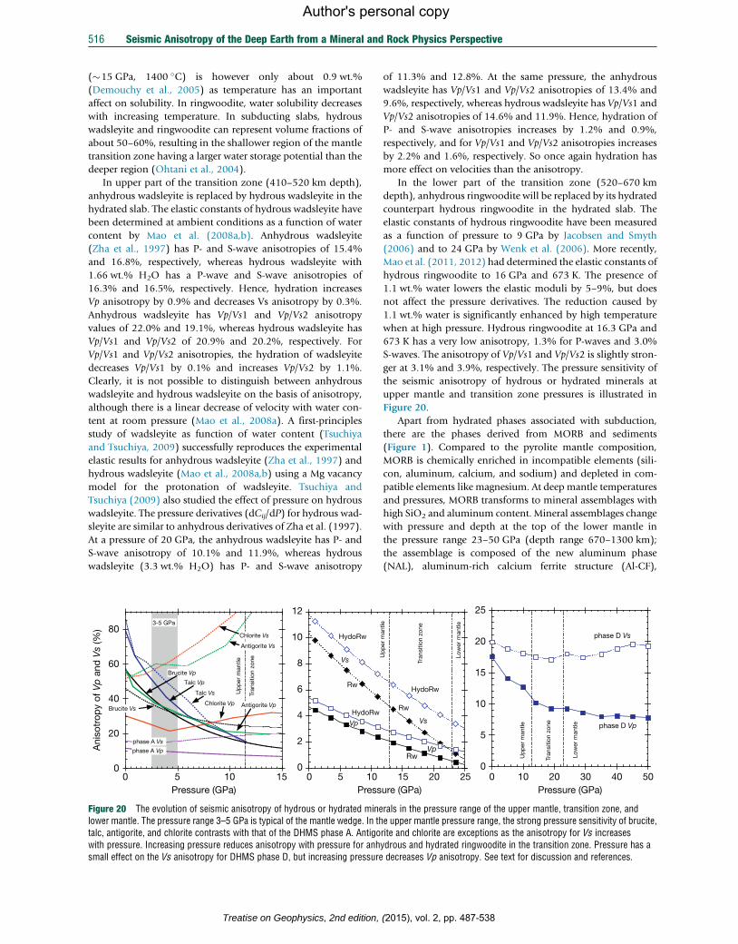
516 Seismic Anisotropy of the Deep Earth from a Mineral and Rock Physics Perspective
Author's personal copy
(�15 GPa, 1400 �C) is however only about 0.9 wt.%
(Demouchy et al., 2005) as temperature has an important
affect on solubility. In ringwoodite, water solubility decreases
with increasing temperature. In subducting slabs, hydrous
wadsleyite and ringwoodite can represent volume fractions of
about 50–60%, resulting in the shallower region of the mantle
transition zone having a larger water storage potential than the
deeper region (Ohtani et al., 2004).
In upper part of the transition zone (410–520 km depth),
anhydrous wadsleyite is replaced by hydrous wadsleyite in the
hydrated slab. The elastic constants of hydrous wadsleyite have
been determined at ambient conditions as a function of water
content by Mao et al. (2008a,b). Anhydrous wadsleyite
(Zha et al., 1997) has P- and S-wave anisotropies of 15.4%
and 16.8%, respectively, whereas hydrous wadsleyite with
1.66 wt.% H2O has a P-wave and S-wave anisotropies of
16.3% and 16.5%, respectively. Hence, hydration increases
Vp anisotropy by 0.9% and decreases Vs anisotropy by 0.3%.
Anhydrous wadsleyite has Vp/Vs1 and Vp/Vs2 anisotropy
values of 22.0% and 19.1%, whereas hydrous wadsleyite has
Vp/Vs1 and Vp/Vs2 of 20.9% and 20.2%, respectively. For
Vp/Vs1 and Vp/Vs2 anisotropies, the hydration of wadsleyite
decreases Vp/Vs1 by 0.1% and increases Vp/Vs2 by 1.1%.
Clearly, it is not possible to distinguish between anhydrous
wadsleyite and hydrous wadsleyite on the basis of anisotropy,
although there is a linear decrease of velocity with water con-
tent at room pressure (Mao et al., 2008a). A first-principles
study of wadsleyite as function of water content (Tsuchiya
and Tsuchiya, 2009) successfully reproduces the experimental
elastic results for anhydrous wadsleyite (Zha et al., 1997) and
hydrous wadsleyite (Mao et al., 2008a,b) using a Mg vacancy
model for the protonation of wadsleyite. Tsuchiya and
Tsuchiya (2009) also studied the effect of pressure on hydrous
wadsleyite. The pressure derivatives (dCij/dP) for hydrous wad-
sleyite are similar to anhydrous derivatives of Zha et al. (1997).
At a pressure of 20 GPa, the anhydrous wadsleyite has P- and
S-wave anisotropy of 10.1% and 11.9%, whereas hydrous
wadsleyite (3.3 wt.% H2O) has P- and S-wave anisotropy
0
2
4
6
8
10
12
0 5 10Press
HydoRw
Vp
Vs
Rw
HydoRw
0
20
40
60
80
0 5 10 15Pressure (GPa)
Brucite Vs
phase A Vs
phase A Vp
Talc Vp
Talc Vs
Brucite Vp
Chlorite Vs
Chlorite Vp
Antigorite Vs
Antigorite Vp
3-5 GPa
Tran
sitio
n zo
ne
Up
per
man
tle
Ani
sotr
opy
of V
p a
nd V
s (%
)
Figure 20 The evolution of seismic anisotropy of hydrous or hydrated minelower mantle. The pressure range 3–5 GPa is typical of the mantle wedge. In thtalc, antigorite, and chlorite contrasts with that of the DHMS phase A. Antigowith pressure. Increasing pressure reduces anisotropy with pressure for anhsmall effect on the Vs anisotropy for DHMS phase D, but increasing pressure
Treatise on Geophysics, 2nd edition,
of 11.3% and 12.8%. At the same pressure, the anhydrous
wadsleyite has Vp/Vs1 and Vp/Vs2 anisotropies of 13.4% and
9.6%, respectively, whereas hydrous wadsleyite has Vp/Vs1 and
Vp/Vs2 anisotropies of 14.6% and 11.9%. Hence, hydration of
P- and S-wave anisotropies increases by 1.2% and 0.9%,
respectively, and for Vp/Vs1 and Vp/Vs2 anisotropies increases
by 2.2% and 1.6%, respectively. So once again hydration has
more effect on velocities than the anisotropy.
In the lower part of the transition zone (520–670 km
depth), anhydrous ringwoodite will be replaced by its hydrated
counterpart hydrous ringwoodite in the hydrated slab. The
elastic constants of hydrous ringwoodite have been measured
as a function of pressure to 9 GPa by Jacobsen and Smyth
(2006) and to 24 GPa by Wenk et al. (2006). More recently,
Mao et al. (2011, 2012) had determined the elastic constants of
hydrous ringwoodite to 16 GPa and 673 K. The presence of
1.1 wt.% water lowers the elastic moduli by 5–9%, but does
not affect the pressure derivatives. The reduction caused by
1.1 wt.% water is significantly enhanced by high temperature
when at high pressure. Hydrous ringwoodite at 16.3 GPa and
673 K has a very low anisotropy, 1.3% for P-waves and 3.0%
S-waves. The anisotropy of Vp/Vs1 and Vp/Vs2 is slightly stron-
ger at 3.1% and 3.9%, respectively. The pressure sensitivity of
the seismic anisotropy of hydrous or hydrated minerals at
upper mantle and transition zone pressures is illustrated in
Figure 20.
Apart from hydrated phases associated with subduction,
there are the phases derived from MORB and sediments
(Figure 1). Compared to the pyrolite mantle composition,
MORB is chemically enriched in incompatible elements (sili-
con, aluminum, calcium, and sodium) and depleted in com-
patible elements like magnesium. At deep mantle temperatures
and pressures, MORB transforms to mineral assemblages with
high SiO2 and aluminum content. Mineral assemblages change
with pressure and depth at the top of the lower mantle in
the pressure range 23–50 GPa (depth range 670–1300 km);
the assemblage is composed of the new aluminum phase
(NAL), aluminum-rich calcium ferrite structure (Al-CF),
0
5
10
15
20
25
0 10 20 30 40 50
phase D Vs
phase D Vp
Tran
sitio
n zo
ne
Low
er m
antle
Up
per
man
tle
Pressure (GPa) 15 20 25
ure (GPa)
Vs
VpRw
Rw
HydoRw
Tran
sitio
n zo
ne
Low
er m
antle
Up
per
man
tle
rals in the pressure range of the upper mantle, transition zone, ande upper mantle pressure range, the strong pressure sensitivity of brucite,rite and chlorite are exceptions as the anisotropy for Vs increasesydrous and hydrated ringwoodite in the transition zone. Pressure has adecreases Vp anisotropy. See text for discussion and references.
(2015), vol. 2, pp. 487-538
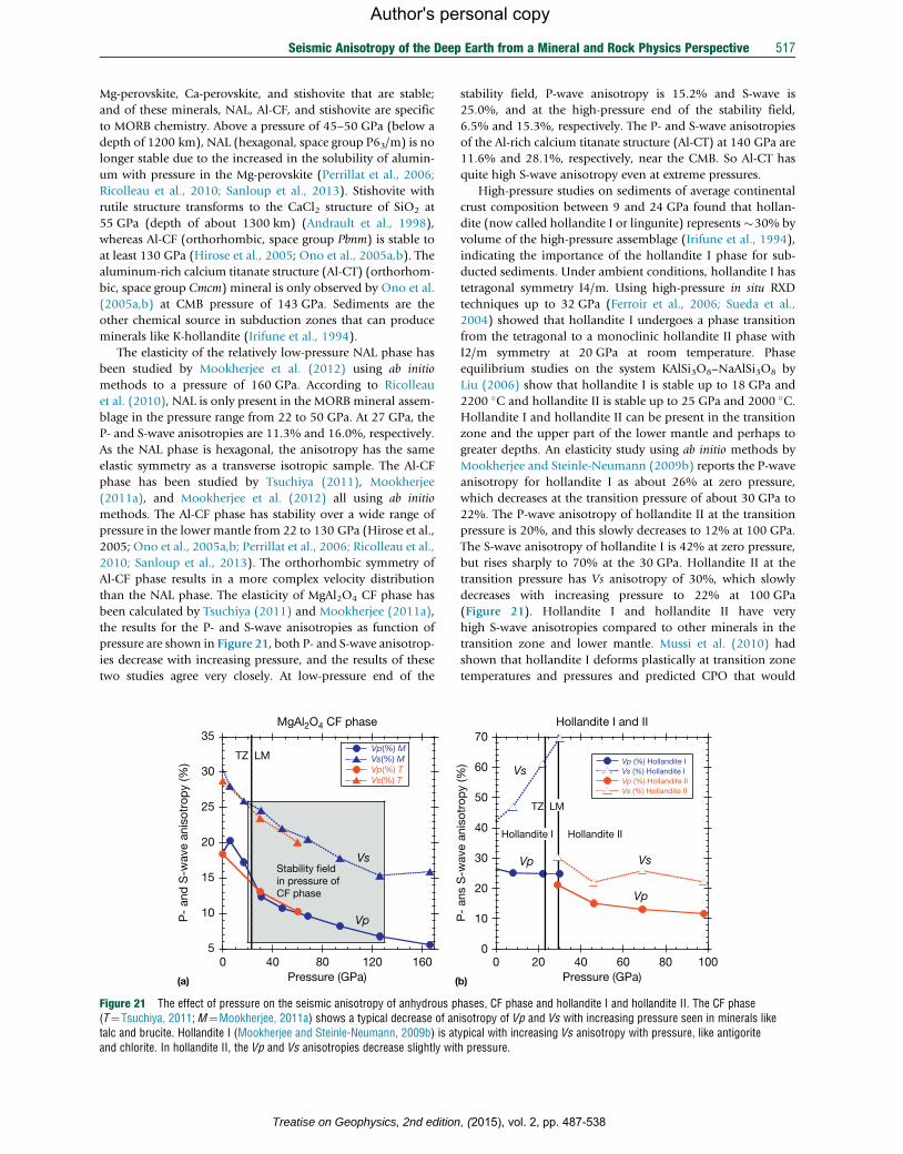
Seismic Anisotropy of the Deep Earth from a Mineral and Rock Physics Perspective 517
Author's personal copy
Mg-perovskite, Ca-perovskite, and stishovite that are stable;
and of these minerals, NAL, Al-CF, and stishovite are specific
to MORB chemistry. Above a pressure of 45–50 GPa (below a
depth of 1200 km), NAL (hexagonal, space group P63/m) is no
longer stable due to the increased in the solubility of alumin-
um with pressure in the Mg-perovskite (Perrillat et al., 2006;
Ricolleau et al., 2010; Sanloup et al., 2013). Stishovite with
rutile structure transforms to the CaCl2 structure of SiO2 at
55 GPa (depth of about 1300 km) (Andrault et al., 1998),
whereas Al-CF (orthorhombic, space group Pbnm) is stable to
at least 130 GPa (Hirose et al., 2005; Ono et al., 2005a,b). The
aluminum-rich calcium titanate structure (Al-CT) (orthorhom-
bic, space group Cmcm) mineral is only observed by Ono et al.
(2005a,b) at CMB pressure of 143 GPa. Sediments are the
other chemical source in subduction zones that can produce
minerals like K-hollandite (Irifune et al., 1994).
The elasticity of the relatively low-pressure NAL phase has
been studied by Mookherjee et al. (2012) using ab initio
methods to a pressure of 160 GPa. According to Ricolleau
et al. (2010), NAL is only present in the MORB mineral assem-
blage in the pressure range from 22 to 50 GPa. At 27 GPa, the
P- and S-wave anisotropies are 11.3% and 16.0%, respectively.
As the NAL phase is hexagonal, the anisotropy has the same
elastic symmetry as a transverse isotropic sample. The Al-CF
phase has been studied by Tsuchiya (2011), Mookherjee
(2011a), and Mookherjee et al. (2012) all using ab initio
methods. The Al-CF phase has stability over a wide range of
pressure in the lower mantle from 22 to 130 GPa (Hirose et al.,
2005; Ono et al., 2005a,b; Perrillat et al., 2006; Ricolleau et al.,
2010; Sanloup et al., 2013). The orthorhombic symmetry of
Al-CF phase results in a more complex velocity distribution
than the NAL phase. The elasticity of MgAl2O4 CF phase has
been calculated by Tsuchiya (2011) and Mookherjee (2011a),
the results for the P- and S-wave anisotropies as function of
pressure are shown in Figure 21, both P- and S-wave anisotrop-
ies decrease with increasing pressure, and the results of these
two studies agree very closely. At low-pressure end of the
5
10
15
20
25
30
35
0 40 80 120 160
MgAl2O4 CF phase
Vp(%) M Vs(%) M Vp(%) T Vs(%) T
P-
and
S-w
ave
anis
otro
py
(%)
Pressure (GPa)
Vp
VsStability fieldin pressure ofCF phase
(a) (
TZ LM
Figure 21 The effect of pressure on the seismic anisotropy of anhydrous p(T¼Tsuchiya, 2011; M¼Mookherjee, 2011a) shows a typical decrease of antalc and brucite. Hollandite I (Mookherjee and Steinle-Neumann, 2009b) is atand chlorite. In hollandite II, the Vp and Vs anisotropies decrease slightly wit
Treatise on Geophysics, 2nd edition
stability field, P-wave anisotropy is 15.2% and S-wave is
25.0%, and at the high-pressure end of the stability field,
6.5% and 15.3%, respectively. The P- and S-wave anisotropies
of the Al-rich calcium titanate structure (Al-CT) at 140 GPa are
11.6% and 28.1%, respectively, near the CMB. So Al-CT has
quite high S-wave anisotropy even at extreme pressures.
High-pressure studies on sediments of average continental
crust composition between 9 and 24 GPa found that hollan-
dite (now called hollandite I or lingunite) represents �30% by
volume of the high-pressure assemblage (Irifune et al., 1994),
indicating the importance of the hollandite I phase for sub-
ducted sediments. Under ambient conditions, hollandite I has
tetragonal symmetry I4/m. Using high-pressure in situ RXD
techniques up to 32 GPa (Ferroir et al., 2006; Sueda et al.,
2004) showed that hollandite I undergoes a phase transition
from the tetragonal to a monoclinic hollandite II phase with
I2/m symmetry at 20 GPa at room temperature. Phase
equilibrium studies on the system KAlSi3O8–NaAlSi3O8 by
Liu (2006) show that hollandite I is stable up to 18 GPa and
2200 �C and hollandite II is stable up to 25 GPa and 2000 �C.Hollandite I and hollandite II can be present in the transition
zone and the upper part of the lower mantle and perhaps to
greater depths. An elasticity study using ab initio methods by
Mookherjee and Steinle-Neumann (2009b) reports the P-wave
anisotropy for hollandite I as about 26% at zero pressure,
which decreases at the transition pressure of about 30 GPa to
22%. The P-wave anisotropy of hollandite II at the transition
pressure is 20%, and this slowly decreases to 12% at 100 GPa.
The S-wave anisotropy of hollandite I is 42% at zero pressure,
but rises sharply to 70% at the 30 GPa. Hollandite II at the
transition pressure has Vs anisotropy of 30%, which slowly
decreases with increasing pressure to 22% at 100 GPa
(Figure 21). Hollandite I and hollandite II have very
high S-wave anisotropies compared to other minerals in the
transition zone and lower mantle. Mussi et al. (2010) had
shown that hollandite I deforms plastically at transition zone
temperatures and pressures and predicted CPO that would
0
10
20
30
40
50
60
70
0 20 40 60 80 100
Hollandite I and II
Vp (%) Hollandite IVs (%) Hollandite IVp (%) Hollandite IIVs (%) Hollandite II
P-
ans
S-w
ave
anis
otro
py
(%)
Pressure (GPa)b)
Vs
Vp
Vp
Vs
Hollandite I Hollandite II
TZ LM
hases, CF phase and hollandite I and hollandite II. The CF phaseisotropy of Vp and Vs with increasing pressure seen in minerals likeypical with increasing Vs anisotropy with pressure, like antigoriteh pressure.
, (2015), vol. 2, pp. 487-538
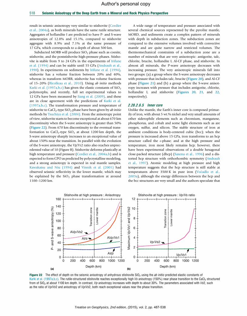
518 Seismic Anisotropy of the Deep Earth from a Mineral and Rock Physics Perspective
Author's personal copy
result in seismic anisotropy very similar to stishovite (Cordier
et al., 2004a), as both minerals have the same rutile structure.
Aggregates of hollandite I are predicted to have P- and S-wave
anisotropies of 12.8% and 15.1%, compared to stishovite
aggregate with 8.9% and 7.1% at the same pressure of
17 GPa, which corresponds to a depth of about 500 km.
Subducted MORB will produce SiO2 phase such as coesite,
stishovite, and the poststishovite high-pressure phases. Stisho-
vite is stable from 9 to 24 GPa in the experiments of Irifune
et al. (1994) and can be stable until 55 GPa (Andrault et al.,
1998). In experiments on sediments by Irifune et al. (1994),
stishovite has a volume fraction between 20% and 40%,
whereas in transform MORB, stishovite has volume fractions
of 15–20% (Ricolleau et al., 2010). Using ab initio methods
Karki et al. (1997a,b,c) has given the elastic constants of SiO2
polymorphs, and recently, full set experimental values to
12 GPa have been measured by Jiang et al. (2009), and these
are in close agreement with the predictions of Karki et al.
(1997a,b,c). The transformation pressure and temperature of
stishovite to CaCl2-type SiO2 phase have been given by ab initio
methods by Tsuchiya et al. (2004). From the anisotropy point
of view, stishovite starts to become exceptional at about 670 km
discontinuity when the S-wave anisotropy is greater than 50%
(Figure 22). From 670 km discontinuity to the eventual trans-
formation to CaCl2-type SiO2 at about 1200 km depth, the
S-wave anisotropy sharply increases to an exceptional value of
about 150% near the transition. In parallel with the evolution
of the S-wave anisotropy, the Vp/Vs2 ratio also reaches unprec-
edented value of 10 (Figure B). Stishovite deforms plastically at
high temperature and pressure (Cordier et al., 2004a,b) and is
expected to formCPOas predicted by polycrystallinemodeling,
and a strong anisotropy is expected in real mantle samples.
Kawakatsu and Niu (1994) and Vinnik et al. (2001) had
observed seismic reflectivity in the lower mantle, which may
be explained by the SiO2 phase transformation at around
1100–1200 km.
0
20
40
60
80
100
120
140
160
0 200 400 600 800 1000 1200
Stishovite at high pressure : Anisotropy
P-
and
S-w
ave
anis
otro
py
(%)
Depth (km)
AVs AVp/Vs1
AVp
AVp/Vs2
Tran
sitio
n zo
ne
Low
er m
antle
(a) (
Figure 22 The effect of depth on the seismic anisotropy of anhydrous stishKarki et al. (1997a,b,c). The rutile-structured stishovite reaches exceptionallyfrom of SiO2 at about 1100 km depth. In contrast, Vp anisotropy increases was the ratio of Vp/Vs2 and anisotropy of Vp/Vs2, both reach exceptional value
Treatise on Geophysics, 2nd edition,
A wide range of temperature and pressure associated with
several chemical sources represented by the pyrolite mantle,
MORD, and sediments create a complex pattern of minerals
with depth in subduction zones. The subduction zones are
compared to the extensive volumes involved with convective
mantle and are quite narrow and restricted volumes. The
thermomechanical constraints of a subduction zone are a
number of minerals that are very anisotropic: antigorite, talc,
chlorite, brucite, hollandite I, Al-CF phase, and stishovite. In
almost all minerals, the P-wave anisotropy decreases with
increasing pressure. The very anisotropic minerals fall into
two groups: (a) a group where the S-wave anisotropy decreases
with pressure that includes talc, brucite (Figure 20), and Al-CF
phase (Figure 21) and (b) a group where the S-wave anisot-
ropy increases with pressure that includes antigorite, chlorite,
hollandite I, and stishovite (Figures 20, 21, and 22,
respectively).
2.20.2.6.5 Inner coreUnlike the mantle, the Earth’s inner core is composed primar-
ily of iron, with about 5 wt.% nickel and very small amounts of
other siderophile elements such as chromium, manganese,
phosphorus, and cobalt and some light elements such as are
oxygen, sulfur, and silicon. The stable structure of iron at
ambient conditions is body-centered cubic (bcc); when the
pressure is increased above 15 GPa, iron transforms to an hcp
structure called the e-phase; and at the high pressure and
temperature, iron most likely remains hcp; however, there
have been experimental observations of a double hexagonal
close-packed structure (dhcp) (Saxena et al., 1996) and a dis-
torted hcp structure with orthorhombic symmetry (Andrault
et al., 1997). Atomic modeling at high pressure and high
temperature suggests that the hcp structure is still stable at
temperatures above 3500 K in pure iron (Vocadlo et al.,
2003a), although the energy differences between the hcp and
the bcc structures are very small and the authors speculate that
0
2
4
6
8
10
12
0 200 400 600 800 1000 1200
Stishovite at high pressure : Vp/Vs ratio
Depth (km)
Vp/Vs2
Vp/Vs1
Max
imum
Vp
/Vs1
and
Vp
/Vs2
b)
Tran
sitio
n zo
ne
Low
er m
antle
ovite SiO2 using the ab initio predicted elastic constants ofhigh Vs anisotropy (150%) near phase transition to the CaCl2 structuredith depth to about 30%. The parameters associated with Vs2, suchs near the phase transition.
(2015), vol. 2, pp. 487-538
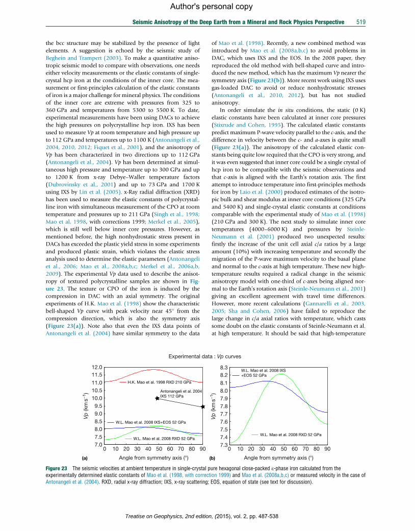
Seismic Anisotropy of the Deep Earth from a Mineral and Rock Physics Perspective 519
Author's personal copy
the bcc structure may be stabilized by the presence of light
elements. A suggestion is echoed by the seismic study of
Beghein and Trampert (2003). To make a quantitative aniso-
tropic seismic model to compare with observations, one needs
either velocity measurements or the elastic constants of single-
crystal hcp iron at the conditions of the inner core. The mea-
surement or first-principles calculation of the elastic constants
of iron is a major challenge for mineral physics. The conditions
of the inner core are extreme with pressures from 325 to
360 GPa and temperatures from 5300 to 5500 K. To date,
experimental measurements have been using DACs to achieve
the high pressures on polycrystalline hcp iron. IXS has been
used to measure Vp at room temperature and high pressure up
to 112 GPa and temperatures up to 1100 K (Antonangeli et al.,
2004, 2010, 2012; Fiquet et al., 2001), and the anisotropy of
Vp has been characterized in two directions up to 112 GPa
(Antonangeli et al., 2004). Vp has been determined at simul-
taneous high pressure and temperature up to 300 GPa and up
to 1200 K from x-ray Debye–Waller temperature factors
(Dubrovinsky et al., 2001) and up to 73 GPa and 1700 K
using IXS by Lin et al. (2005). x-Ray radial diffraction (XRD)
has been used to measure the elastic constants of polycrystal-
line iron with simultaneous measurement of the CPO at room
temperature and pressures up to 211 GPa (Singh et al., 1998;
Mao et al, 1998, with corrections 1999; Merkel et al., 2005),
which is still well below inner core pressures. However, as
mentioned before, the high nonhydrostatic stress present in
DACs has exceeded the plastic yield stress in some experiments
and produced plastic strain, which violates the elastic stress
analysis used to determine the elastic parameters (Antonangeli
et al., 2006; Mao et al., 2008a,b,c; Merkel et al., 2006a,b,
2009). The experimental Vp data used to describe the anisot-
ropy of textured polycrystalline samples are shown in Fig-
ure 23. The texture or CPO of the iron is induced by the
compression in DAC with an axial symmetry. The original
experiments of H.K. Mao et al. (1998) show the characteristic
bell-shaped Vp curve with peak velocity near 45� from the
compression direction, which is also the symmetry axis
(Figure 23(a)). Note also that even the IXS data points of
Antonangeli et al. (2004) have similar symmetry to the data
Experimental dat
0 10 20 30 40 50 60 70 80 907.07.58.08.59.09.5
10.010.511.0
11.512.0
Angle from symmetry axis (°)
Vp
(km
s−1)
H.K. Mao et al. 1998 RXD 210 GPa
Antonangeli et al. 2004 IXS 112 GPa
W.L. Mao et al. 2008 RXD 52 GPa
W.L. Mao et al. 2008 IXS+EOS 52 GPa
(a) (
Figure 23 The seismic velocities at ambient temperature in single-crystal pexperimentally determined elastic constants of Mao et al. (1998, with correctAntonangeli et al. (2004). RXD, radial x-ray diffraction; IXS, x-ray scattering;
Treatise on Geophysics, 2nd edition
of Mao et al. (1998). Recently, a new combined method was
introduced by Mao et al. (2008a,b,c) to avoid problems in
DAC, which uses IXS and the EOS. In the 2008 paper, they
reproduced the old method with bell-shaped curve and intro-
duced the new method, which has the maximum Vp nearer the
symmetry axis (Figure 23(b)). More recent work using IXS uses
gas-loaded DAC to avoid or reduce nonhydrostatic stresses
(Antonangeli et al., 2010, 2012), but has not studied
anisotropy.
In order simulate the in situ conditions, the static (0 K)
elastic constants have been calculated at inner core pressures
(Stixrude and Cohen, 1995). The calculated elastic constants
predict maximum P-wave velocity parallel to the c-axis, and the
difference in velocity between the c- and a-axes is quite small
(Figure 23(a)). The anisotropy of the calculated elastic con-
stants being quite low required that the CPO is very strong, and
it was even suggested that inner core could be a single crystal of
hcp iron to be compatible with the seismic observations and
that c-axis is aligned with the Earth’s rotation axis. The first
attempt to introduce temperature into first-principles methods
for iron by Laio et al. (2000) produced estimates of the isotro-
pic bulk and shear modulus at inner core conditions (325 GPa
and 5400 K) and single-crystal elastic constants at conditions
comparable with the experimental study of Mao et al. (1998)
(210 GPa and 300 K). The next study to simulate inner core
temperatures (4000–6000 K) and pressures by Steinle-
Neumann et al. (2001) produced two unexpected results:
firstly the increase of the unit cell axial c/a ratios by a large
amount (10%) with increasing temperature and secondly the
migration of the P-wave maximum velocity to the basal plane
and normal to the c-axis at high temperature. These new high-
temperature results required a radical change in the seismic
anisotropy model with one-third of c-axes being aligned nor-
mal to the Earth’s rotation axis (Steinle-Neumann et al., 2001)
giving an excellent agreement with travel time differences.
However, more recent calculations (Gannarelli et al., 2003,
2005; Sha and Cohen, 2006) have failed to reproduce the
large change in c/a axial ratios with temperature, which casts
some doubt on the elastic constants of Steinle-Neumann et al.
at high temperature. It should be said that high-temperature
a : Vp curves
0 10 20 30 40 50 60 70 80 90
Angle from symmetry axis (°)
7.37.47.57.67.77.87.98.08.1
8.28.3
Vp
(km
s−1)
W.L. Mao et al. 2008 IXS+EOS 52 GPa
W.L. Mao et al. 2008 RXD 52 GPa
b)
ure hexagonal close-packed e-phase iron calculated from theion 1999) and Mao et al. (2008a,b,c) or measured velocity in the case ofEOS, equation of state (see text for discussion).
, (2015), vol. 2, pp. 487-538
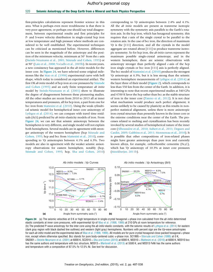
520 Seismic Anisotropy of the Deep Earth from a Mineral and Rock Physics Perspective
Author's personal copy
first-principles calculations represent frontier science in this
area. What is perhaps even more troublesome is that there is
very poor agreement, or perhaps one should say total disagree-
ment, between experimental results and first principles for
P- and S-wave velocity distribution in single-crystal hcp iron
at low temperature and high pressure where methods are con-
sidered to be well established. The experimental techniques
can be criticized as mentioned before. However, differences
can be seen in the magnitude of the anisotropy and the posi-
tion of the minimum velocity, minimum at 50� from the c-axis
(Steinle-Neumann et al., 2001; Stixrude and Cohen, 1995) or
at 90� (Laio et al., 2000; Vocadlo et al., 2003b). In recent years,
a new consistency has appeared in the ab initio models for the
inner core. In Figure 24, we have selected some original mile-
stones like the Mao et al. (1998) experimental curve with bell
shape, which today is considered an experimental artifact. The
first OK ab initiomodel of hcp iron at core pressures by Stixrude
and Cohen (1995) and an early finite temperature ab initio
model by Steinle-Neumann et al. (2001) show to illustrate
the degree of disagreement between these pioneering studies.
All the other studies are recent from 2010 to 2013 all at inner
temperatures and pressures, all for hcp iron, a part from one for
bcc iron from Mattesini et al. (2010). Using the weak cylindri-
cal seismic model for hemispherical inner core anisotropy of
Lythgoe et al. (2014), we can compare with travel time resid-
uals (dt/t) predicted by ab initio elasticity models of iron. From
Figure 24, we can see that seismic anisotropy between the
hemispheres is very different, and single model will not explain
both hemispheres. Several models are in agreement with stron-
ger anisotropy of the western hemisphere (hcp Stixrude and
Cohen, 1995; hcp and bcc from Mattesini et al., 2010), corre-
sponding to Vp anisotropies between 4.1% and 6.3%. Two
models are also in agreement with the weaker seismic anisot-
ropy observations for eastern hemisphere, notably (hcp,
Stixrude and Cohen, 1995; hcp, Sha and Cohen, 2010)
10.0
10.5
11.0
11.5
12.0
12.5
13.0
Ab initio models : Vp Curves
0 10 20 30 40 50 60 70 80 90
Angle from symmetry axis (°)
Vp
(km
s−1)
SN2001
M1998 RXD
SC1995
M2010
M2010 bcc
M2013M2013 FeNi
SC2010
4.1%
20.5%
7.2%
8.3%7.5%
6.3%
5.7%
2.4%
((a)
Figure 24 (a) The seismic velocities at 0 K or high temperature in single-crelastic constants at inner core pressures, with experimental Vp of Mao et al.(b) The predicted P-wave anisotropy for the inter core using the ab initio elast(dark gray region with black dashed line outlines) and western (light gray) hefor each ab initiomodel and the experimental data of Mao et al. (1998, 1999). Airon, except where otherwise specified. Bcc stands for pure body-centered cuSN2001¼Steinle-Neumann et al. (2001) at 6000 K, SC2010¼Sha and Cohenhas the same authors and temperature with bcc structure, M2013¼Martoreland temperature with a composition of 87.5% Fe 12.5% Ni. See text for disc
Treatise on Geophysics, 2nd edition,
corresponding to Vp anisotropies between 2.4% and 4.1%.
All the ab initio models are present as transverse isotropic
symmetry with the symmetry axis parallels to the Earth’s rota-
tion axis. In the hcp iron, which has hexagonal symmetry, this
requires that c-axis of the single crystal to be parallel to the
rotation axis. In the case of bcc iron, the direction of maximum
Vp is the [111] direction, and all the crystals in the model
aggregate are rotated about [111] to produce transverse isotro-
pic symmetry. So for hcp iron, the ab initio curves represent the
maximum possible single-crystal anisotropy, and in the
western hemisphere, there are seismic observations with
anisotropy stronger than perfectly aligned c-axis of the hcp
iron single crystals or bcc iron [111] axis is perfectly aligned.
The bcc model of Mattesini et al. (2010) produces the strongest
Vp anisotropy at 6.3%, but it is less strong than the seismic
western hemisphere measurements of Lythgoe et al. (2014) at
the layer three of their model (Figure 2), which corresponds to
less than 550 km from the center of the Earth. In addition, it is
interesting to note that recent experimental studies at 340 GPa
and 4700 K favor the hcp rather than bcc as the stable structure
of iron in the inner core (Tateno et al., 2012). It is not clear
what mechanism would produce such perfect alignment; it
seems unlikely to be caused by plasticity as this results in non-
perfect statistical alignment, unless there is more anisotropic
iron crystal structure than presently known in the inner core or
the extreme conditions near the center of the Earth. The pro-
cesses related to melting and crystallization has been recently
invoked by several studies of hemispherical nature of the inner
core (Alboussiere et al., 2010; Aubert et al., 2011; Deguen and
Cardin, 2009; Gubbins et al., 2011; Monnereau et al., 2010). It
is possible that other compositions of iron-related phases
might have greater anisotropy than pure iron and currently
known alloys, for example, orthorhombic cementite (Fe3C),
which has Vp anisotropy of 10.3% at inner core pressures
(Mookherjee, 2011b).
0 10 20 30 40 50 60 70 80 90
Angle from symmetry axis (°)
Ab initio models : Vp Anisotropy (δt/t)
−0.15
−0.10
−0.05
0.05
0.10
Vp
Ani
sotr
opy
(δt/
t)
0.00SC2010 2.4%
SN2001 20.5% M2013M2013 FeNi
8.3%7.5%
M2010M2010 bcc
6.3%5.7%
SC1995
4.1%
Isotropic
b)
Eastern
Western
ystal hexagonal e-phase iron calculated from the ab initio determined(1998, 1999) at 210 GPa at room temperature for reference.ic constants, with the seismic results of Lythgoe et al. (2014) for easternmispheres. Numbers with percent sign are the Vp-wave anisotropiesll models are for pure crystal hexagonal close-packed hexagonal e-phasebic a-phase iron. SC1995¼Stixrude and Cohen (1995) at 0 K,(2010) at 6000 K, M2010¼Mattesini et al. (2010) at 6000 K, M2010 bccl et al. (2013) at 5500 K, and M2013 FeNi has the same authorsussion.
(2015), vol. 2, pp. 487-538
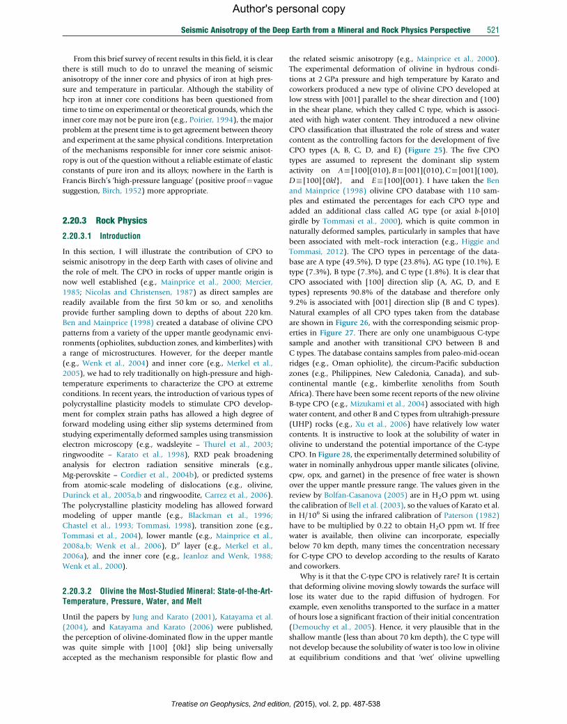
Seismic Anisotropy of the Deep Earth from a Mineral and Rock Physics Perspective 521
Author's personal copy
From this brief survey of recent results in this field, it is clear
there is still much to do to unravel the meaning of seismic
anisotropy of the inner core and physics of iron at high pres-
sure and temperature in particular. Although the stability of
hcp iron at inner core conditions has been questioned from
time to time on experimental or theoretical grounds, which the
inner core may not be pure iron (e.g., Poirier, 1994), the major
problem at the present time is to get agreement between theory
and experiment at the same physical conditions. Interpretation
of the mechanisms responsible for inner core seismic anisot-
ropy is out of the question without a reliable estimate of elastic
constants of pure iron and its alloys; nowhere in the Earth is
Francis Birch’s ‘high-pressure language’ (positive proof¼vague
suggestion, Birch, 1952) more appropriate.
2.20.3 Rock Physics
2.20.3.1 Introduction
In this section, I will illustrate the contribution of CPO to
seismic anisotropy in the deep Earth with cases of olivine and
the role of melt. The CPO in rocks of upper mantle origin is
now well established (e.g., Mainprice et al., 2000; Mercier,
1985; Nicolas and Christensen, 1987) as direct samples are
readily available from the first 50 km or so, and xenoliths
provide further sampling down to depths of about 220 km.
Ben and Mainprice (1998) created a database of olivine CPO
patterns from a variety of the upper mantle geodynamic envi-
ronments (ophiolites, subduction zones, and kimberlites) with
a range of microstructures. However, for the deeper mantle
(e.g., Wenk et al., 2004) and inner core (e.g., Merkel et al.,
2005), we had to rely traditionally on high-pressure and high-
temperature experiments to characterize the CPO at extreme
conditions. In recent years, the introduction of various types of
polycrystalline plasticity models to stimulate CPO develop-
ment for complex strain paths has allowed a high degree of
forward modeling using either slip systems determined from
studying experimentally deformed samples using transmission
electron microscopy (e.g., wadsleyite – Thurel et al., 2003;
ringwoodite – Karato et al., 1998), RXD peak broadening
analysis for electron radiation sensitive minerals (e.g.,
Mg-perovskite – Cordier et al., 2004b), or predicted systems
from atomic-scale modeling of dislocations (e.g., olivine,
Durinck et al., 2005a,b and ringwoodite, Carrez et al., 2006).
The polycrystalline plasticity modeling has allowed forward
modeling of upper mantle (e.g., Blackman et al., 1996;
Chastel et al., 1993; Tommasi, 1998), transition zone (e.g.,
Tommasi et al., 2004), lower mantle (e.g., Mainprice et al.,
2008a,b; Wenk et al., 2006), D00 layer (e.g., Merkel et al.,
2006a), and the inner core (e.g., Jeanloz and Wenk, 1988;
Wenk et al., 2000).
2.20.3.2 Olivine the Most-Studied Mineral: State-of-the-Art-Temperature, Pressure, Water, and Melt
Until the papers by Jung and Karato (2001), Katayama et al.
(2004), and Katayama and Karato (2006) were published,
the perception of olivine-dominated flow in the upper mantle
was quite simple with [100] {0kl} slip being universally
accepted as the mechanism responsible for plastic flow and
Treatise on Geophysics, 2nd edition
the related seismic anisotropy (e.g., Mainprice et al., 2000).
The experimental deformation of olivine in hydrous condi-
tions at 2 GPa pressure and high temperature by Karato and
coworkers produced a new type of olivine CPO developed at
low stress with [001] parallel to the shear direction and (100)
in the shear plane, which they called C type, which is associ-
ated with high water content. They introduced a new olivine
CPO classification that illustrated the role of stress and water
content as the controlling factors for the development of five
CPO types (A, B, C, D, and E) (Figure 25). The five CPO
types are assumed to represent the dominant slip system
activity on A� [100](010),B� [001](010),C� [001](100),
D� [100]{0kl}, and E� [100](001). I have taken the Ben
and Mainprice (1998) olivine CPO database with 110 sam-
ples and estimated the percentages for each CPO type and
added an additional class called AG type (or axial b-[010]
girdle by Tommasi et al., 2000), which is quite common in
naturally deformed samples, particularly in samples that have
been associated with melt–rock interaction (e.g., Higgie and
Tommasi, 2012). The CPO types in percentage of the data-
base are A type (49.5%), D type (23.8%), AG type (10.1%), E
type (7.3%), B type (7.3%), and C type (1.8%). It is clear that
CPO associated with [100] direction slip (A, AG, D, and E
types) represents 90.8% of the database and therefore only
9.2% is associated with [001] direction slip (B and C types).
Natural examples of all CPO types taken from the database
are shown in Figure 26, with the corresponding seismic prop-
erties in Figure 27. There are only one unambiguous C-type
sample and another with transitional CPO between B and
C types. The database contains samples from paleo-mid-ocean
ridges (e.g., Oman ophiolite), the circum-Pacific subduction
zones (e.g., Philippines, New Caledonia, Canada), and sub-
continental mantle (e.g., kimberlite xenoliths from South
Africa). There have been some recent reports of the new olivine
B-type CPO (e.g., Mizukami et al., 2004) associated with high
water content, and other B and C types from ultrahigh-pressure
(UHP) rocks (e.g., Xu et al., 2006) have relatively low water
contents. It is instructive to look at the solubility of water in
olivine to understand the potential importance of the C-type
CPO. In Figure 28, the experimentally determined solubility of
water in nominally anhydrous upper mantle silicates (olivine,
cpw, opx, and garnet) in the presence of free water is shown
over the upper mantle pressure range. The values given in the
review by Bolfan-Casanova (2005) are in H2O ppm wt. using
the calibration of Bell et al. (2003), so the values of Karato et al.
in H/106 Si using the infrared calibration of Paterson (1982)
have to be multiplied by 0.22 to obtain H2O ppm wt. If free
water is available, then olivine can incorporate, especially
below 70 km depth, many times the concentration necessary
for C-type CPO to develop according to the results of Karato
and coworkers.
Why is it that the C-type CPO is relatively rare? It is certain
that deforming olivine moving slowly towards the surface will
lose its water due to the rapid diffusion of hydrogen. For
example, even xenoliths transported to the surface in a matter
of hours lose a significant fraction of their initial concentration
(Demouchy et al., 2005). Hence, it very plausible that in the
shallow mantle (less than about 70 km depth), the C type will
not develop because the solubility of water is too low in olivine
at equilibrium conditions and that ‘wet’ olivine upwelling
, (2015), vol. 2, pp. 487-538
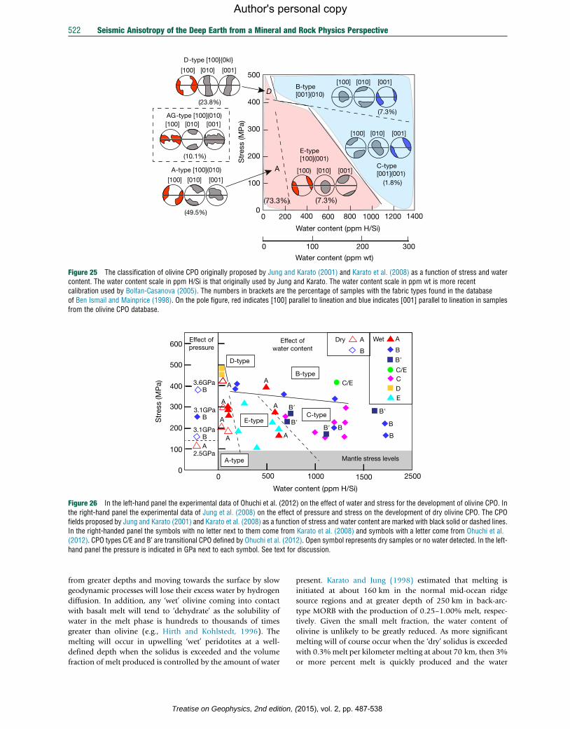
600
500
400
300
200
100
00 500 1000 1500 2500
Str
ess
(MP
a) C/E
B
BB
A
A
A
A
A
A
A
C/E
B
AADry Wet
D-type
B-type
C-typeE-type B�
B�
B�
B�
B�
A-type
Water content (ppm H/Si)
Mantle stress levels2.5GPa
3.1GPa
3.1GPa
3.6GPa
Effect ofpressure B
Effect ofwater content
B
B
BA
C
DE
Figure 26 In the left-hand panel the experimental data of Ohuchi et al. (2012) on the effect of water and stress for the development of olivine CPO. Inthe right-hand panel the experimental data of Jung et al. (2008) on the effect of pressure and stress on the development of dry olivine CPO. The CPOfields proposed by Jung and Karato (2001) and Karato et al. (2008) as a function of stress and water content are marked with black solid or dashed lines.In the right-handed panel the symbols with no letter next to them come from Karato et al. (2008) and symbols with a letter come from Ohuchi et al.(2012). CPO types C/E and B’ are transitional CPO defined by Ohuchi et al. (2012). Open symbol represents dry samples or no water detected. In the left-hand panel the pressure is indicated in GPa next to each symbol. See text for discussion.
500
400
300
200
100
200 400 600 800 1000 1200 1400
B-type[001](010)
C-type[001](001)
E-type[100](001)
A-type [100](010)
D-type [100]{0kl}
Water content (ppm H/Si)
Str
ess
(MP
a)
00
[100] [010] [001]
[100] [010] [001]
[100) [010] [001][100] [010] [001]
[100] [010] [001]
A
D
[100] [010] [001]AG-type [100](010)
(10.1%)
(49.5%)
(23.8%)
(7.3%)
(7.3%)
(73.3%)
(1.8%)
Water content (ppm wt)
2001000 300
Figure 25 The classification of olivine CPO originally proposed by Jung and Karato (2001) and Karato et al. (2008) as a function of stress and watercontent. The water content scale in ppm H/Si is that originally used by Jung and Karato. The water content scale in ppm wt is more recentcalibration used by Bolfan-Casanova (2005). The numbers in brackets are the percentage of samples with the fabric types found in the databaseof Ben Ismail and Mainprice (1998). On the pole figure, red indicates [100] parallel to lineation and blue indicates [001] parallel to lineation in samplesfrom the olivine CPO database.
522 Seismic Anisotropy of the Deep Earth from a Mineral and Rock Physics Perspective
Author's personal copy
from greater depths and moving towards the surface by slow
geodynamic processes will lose their excess water by hydrogen
diffusion. In addition, any ‘wet’ olivine coming into contact
with basalt melt will tend to ‘dehydrate’ as the solubility of
water in the melt phase is hundreds to thousands of times
greater than olivine (e.g., Hirth and Kohlstedt, 1996). The
melting will occur in upwelling ‘wet’ peridotites at a well-
defined depth when the solidus is exceeded and the volume
fraction of melt produced is controlled by the amount of water
Treatise on Geophysics, 2nd edition,
present. Karato and Jung (1998) estimated that melting is
initiated at about 160 km in the normal mid-ocean ridge
source regions and at greater depth of 250 km in back-arc-
type MORB with the production of 0.25–1.00% melt, respec-
tively. Given the small melt fraction, the water content of
olivine is unlikely to be greatly reduced. As more significant
melting will of course occur when the ‘dry’ solidus is exceeded
with 0.3%melt per kilometer melting at about 70 km, then 3%
or more percent melt is quickly produced and the water
(2015), vol. 2, pp. 487-538
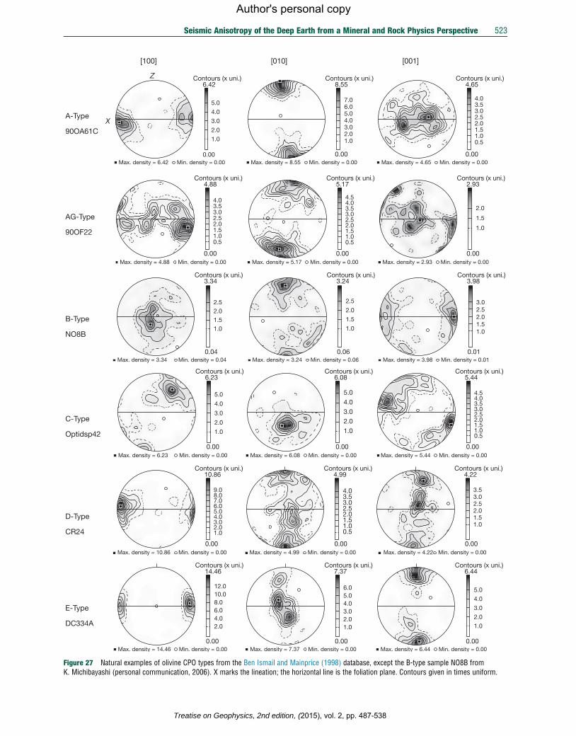
6.42Contours (x uni.)
0.00 Max. density = 6.42 Min. density = 0.00
1.0
2.0
3.0
4.0
5.0
8.55 Contours (x uni.)
0.00 Max. density = 8.55 Min. density = 0.00
1.02.03.04.05.06.07.0
4.65 Contours (x uni.)
0.00 Max. density = 4.65 Min. density = 0.00
0.51.01.52.02.53.03.54.0
[100] [010] [001]
6.23 Contours (x uni.)
0.00 Max. density = 6.23 Min. density = 0.00
1.0
2.0
3.0
4.0
5.0
6.08 Contours (x uni.)
0.00 Max. density = 6.08 Min. density = 0.00
1.0 2.0 3.0 4.0 5.0
5.44 Contours (x uni.)
0.00 Max. density = 5.44 Min. density = 0.00
0.5 1.0 1.5 2.0 2.5 3.0 3.5 4.0 4.5
4.88 Contours (x uni.)
0.00 Max. density = 4.88 Min. density = 0.00
0.5 1.0 1.5 2.0 2.5 3.0 3.5 4.0
5.17 Contours (x uni.)
0.00 Max. density = 5.17 Min. density = 0.00
0.5 1.0 1.5 2.0 2.5 3.0 3.5 4.0 4.5
2.93 Contours (x uni.)
0.00 Max. density = 2.93 Min. density = 0.00
1.0
1.5
2.0
10.86 Contours (x uni.)
0.00 Max. density = 10.86 Min. density = 0.00
1.0 2.0 3.0 4.0 5.0 6.0 7.0 8.0 9.0
4.99 Contours (x uni.)
0.00 Max. density = 4.99 Min. density = 0.00
0.5 1.0 1.5 2.0 2.5 3.0 3.5 4.0
4.22 Contours (x uni.)
0.00 Max. density = 4.22 Min. density = 0.00
1.0 1.5 2.0 2.5 3.0 3.5
E-Type
DC334A
14.46 Contours (x uni.)
0.00 Max. density = 14.46 Min. density = 0.00
2.0 4.0 6.0 8.0 10.0 12.0
7.37 Contours (x uni.)
0.00 Max. density = 7.37 Min. density = 0.00
1.0 2.0 3.0 4.0 5.0 6.0
6.44 Contours (x uni.)
0.00 Max. density = 6.44 Min. density = 0.00
1.0
2.0
3.0
4.0
5.0
D-Type
CR24
C-Type
Optidsp42
B-Type
NO8B
AG-Type
90OF22
A-Type
90OA61CX
Z
3.34 Contours (x uni.)
0.04 Max. density = 3.34 Min. density = 0.04
1.0 1.5 2.0 2.5
3.24 Contours (x uni.)
0.06 Max. density = 3.24 Min. density = 0.06
1.0
1.5
2.0
2.5
3.98 Contours (x uni.)
0.01 Max. density = 3.98 Min. density = 0.01
1.0 1.5 2.0 2.5 3.0
Figure 27 Natural examples of olivine CPO types from the Ben Ismail and Mainprice (1998) database, except the B-type sample NO8B fromK. Michibayashi (personal communication, 2006). X marks the lineation; the horizontal line is the foliation plane. Contours given in times uniform.
Seismic Anisotropy of the Deep Earth from a Mineral and Rock Physics Perspective 523
Treatise on Geophysics, 2nd edition, (2015), vol. 2, pp. 487-538
Author's personal copy
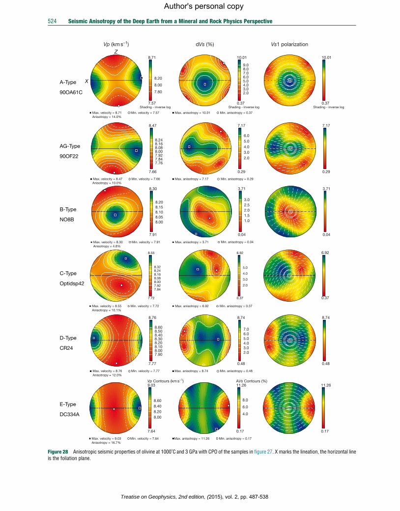
8.71
7.57 Shading - inverse log
Max. velocity = 8.71 Min. velocity = 7.57 Anisotropy = 14.0%
10.01
0.37 Shading - inverse log
Max. anisotropy = 10.01 Min. anisotropy = 0.37
2.0 3.0 4.0 5.0 6.0 7.0 8.0 9.0
10.01
0.37 Shading - inverse log
8.55
7.72
Max. velocity = 8.55 Min. velocity = 7.72 Anisotropy = 10.1%
7.84 7.92 8.00 8.08 8.16 8.24 8.32
6.92
0.37
Max. anisotropy = 6.92 Min. anisotropy = 0.37
2.0
3.0
4.0
5.0
6.92
0.37
8.76
7.77
Max. velocity = 8.76 Min. velocity = 7.77 Anisotropy = 12.0%
7.90 8.00 8.10 8.20 8.30 8.40 8.50 8.60
8.74
0.48
Max. anisotropy = 8.74 Min. anisotropy = 0.48
2.0 3.0 4.0 5.0 6.0 7.0
8.74
0.48
9.03
7.64
Vp Contours (km s−1)
Max. velocity = 9.03 Min. velocity = 7.64 Anisotropy = 16.7%
8.00 8.20 8.40 8.60
11.26
0.17
AVs Contours (%)
Max. anisotropy = 11.26 Min. anisotropy = 0.17
4.0
6.0
8.0
11.26
0.17
8.47
7.66
Max. velocity = 8.47 Min. velocity = 7.66
7.76 7.84 7.92 8.00 8.08 8.16 8.24
7.17
0.29
Max. anisotropy = 7.17 Min. anisotropy = 0.29
2.0 3.0 4.0 5.0 6.0
7.17
0.29
8.30
7.91
Max. velocity = 8.30 Min. velocity = 7.91 Anisotropy = 4.8%
8.00 8.05 8.10 8.15 8.20
3.71
0.04
Max. anisotropy = 3.71 Min. anisotropy = 0.04
1.0 1.5 2.0 2.5 3.0
3.71
0.04
E-Type
DC334A
D-Type
CR24
C-Type
Optidsp42
B-Type
NO8B
AG-Type
90OF22
A-Type
90OA61C
X
Vp (km s−1) dVs (%) Vs1 polarizationZ
7.80
8.00
8.20
Anisotropy = 10.0%
Figure 28 Anisotropic seismic properties of olivine at 1000˚C and 3 GPa with CPO of the samples in figure 27. X marks the lineation, the horizontal lineis the foliation plane.
524 Seismic Anisotropy of the Deep Earth from a Mineral and Rock Physics Perspective
Treatise on Geophysics, 2nd edition, (2015), vol. 2, pp. 487-538
Author's personal copy
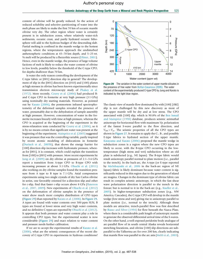
Olivine
Diopside
Enstatite
Pyrop
e
70
120
180
240
300
360
420
0
0
2
4
6
8
10
12
14
0
Pressure (G
Pa)
Dep
th (k
m)
1000 2000 3000 4000
Water content (ppm wt)
Uppermantle
410 km
C-type CPO
Figure 29 The variation in the water content of upper mantle silicates inthe presence of free water from Bolfan-Casanova (2005). The watercontent of the experimentally produced C-type CPO by Jung and Karato isindicated by the light blue region.
Seismic Anisotropy of the Deep Earth from a Mineral and Rock Physics Perspective 525
Author's personal copy
content of olivine will be greatly reduced. So the action of
reduced solubility and selective partitioning of water into the
melt phase are likely to make the first 70 km of oceanic mantle
olivine very dry. The other region where water is certainly
present is in subduction zones, where relatively water-rich
sediments, oceanic crust, and partly hydrated oceanic litho-
sphere will add to the hydrous budget of the descending slab.
Partial melting is confined in the mantle wedge to the hottest
regions, where the temperatures approach the undisturbed
asthenospheric conditions at 45–70 km depth, and 5–25 wt.
%melt will be produced by a lherzolitic source (Ulmer, 2001).
Hence, even in the mantle wedge, the presence of large volume
factions of melt is likely to reduce the water content of olivine
to low levels, possibly below the threshold of the C-type CPO,
for depths shallower than 70 km.
Is water the only reason controlling the development of the
C-type fabric or [001] direction slip in general? The develop-
ment of slip in the [001] direction on (010) and (100) planes
at high stresses in olivine has been known experimentally since
transmission electron microscopy study of Phakey et al.
(1972). More recently, Couvy et al. (2004) had produced B-
and C-type CPO in forsterite at very high pressure (11 GPa)
using nominally dry starting materials. However, as pointed
out by Karato (2006), the postmortem infrared spectropho-
tometry of the deformed samples revealed the presence of
water, presumably due to the dehydration of sample assembly
at high pressure. However, concentration of water in the for-
sterite increases linearly with time at high pressure, whereas the
CPO is acquired at the beginning of the experiment in the
stress-relaxation tests conducted by Couvy et al. (2004), so it
is by no means certain that significant water was present at the
beginning of the experiment. Mainprice et al. (2005) suggested
it was pressure that was the controlling variable, partly inspired
by recent atomic modeling of dislocations in forsterite
(Durinck et al., 2005b), that shows the energy barrier for
[100] direction slip increases with hydrostatic pressure, where-
as for [001], it is constant, which could explain the transition
from [100] to [001] with pressure. More recent experiments by
Jung et al. (2009) on dry olivine at pressures of 2.1–3.6 GPa
report a transition from A-type CPO to B-type CPO with
increasing pressure at about 3.1 GPa. Ohuchi et al. (2011)
also working on dry olivine samples found the transition pres-
sure from A type to B type is 7.1 GPa. Axial compression
experiments using two single crystals of dry San Carlos olivine
in series, one favorably oriented for a-direction slip and other
for c-slip, find that faster c-slip occurs above 8 GPa (Raterron
et al., 2007, 2009). New experiments of Ohuchi et al. (2012)
on the deformation of olivine samples in the presence of
water show much more complex distribution of CPO types
(Figure 29) than reported by Karato et al. (2008). In Figure 29,
A types are found with water contents over 500 ppm H/Si, B
types are found at lower stress and very high water contents,
and no definitive C types are reported by Ohuchi et al. (2012).
It appears that both pressure and water content play a role in
controlling CPO types, but the experimental scatter is now
considerable (Figure 29) and exact relation to water content
and pressure needs further calibration.
If we are to accept the experimental results of Karato et al.
(2008), what are the seismic consequences of the recent dis-
covery of C-type CPO in experiments in hydrous conditions?
Treatise on Geophysics, 2nd edition
The classic view of mantle flow dominated by with [100] {0kl}
slip is not challenged by this new discovery as most of
the upper mantle will be dry and at low stress. The CPO
associated with [100] slip, which is 90.8% of the Ben Ismaıl
and Mainprice (1998) database, produces seismic azimuthal
anisotropy for horizontal flow with maximum Vp, polarization
of the fastest S-wave parallel to the flow direction, and
VSH>Vsv. The seismic properties of all the CPO types are
shown in Figure 27. It remains to apply the C-, B-, and possibly
E-type fabrics to hydrated section of the upper mantle.
Katayama and Karato (2006) proposed the mantle wedge in
subduction zones is a region where the new CPO types are
likely to occur, with the B-type CPO occurring in the low-
temperature (high stress and wet) subduction where an old
plate is subducted (e.g., NE Japan). The B-type fabric would
result anisotropy parallel normal to plate motion (i.e., parallel
to the trench). In the back-arc, the A-type (or E-type reported
by Michibayashi et al., 2006 in the back-arc region of NE
Japan) fabric is likely dominant because water content is sig-
nificantly reduced in this region due to the generation of island
arc magma. Changes in the dominant type of olivine fabric can
result in complex seismic anisotropy, in which the fast shear
wave polarization direction is parallel to the trench in the
forearc but is normal to it in the back-arc (e.g., Kneller et al.,
2005). In higher-temperature subduction zones (e.g., NW
America, Cascades), the C-type CPO will develop in the mantle
wedge (low stress and wet) giving rise to anisotropy parallel to
plate motion (i.e., normal to the trench). Although these
models are attractive, trench-parallel flow was first described
by Russo and Silver (1994) for flow beneath the Nazca Plate,
where there is a considerable path length of anisotropic mantle
to generate the observed differential arrival time of the S-waves.
On the other hand, a well-exposed peridotite body analogue of
arc-parallel flow of in south central Alaska reveals horizontal
stretching lineations, and olivine [100] slip directions are sub-
parallel to the Talkeetna arc for over 200 km, clearly indicating
that mantle flow was parallel to the arc axis (Mehl et al., 2003).
, (2015), vol. 2, pp. 487-538
526 Seismic Anisotropy of the Deep Earth from a Mineral and Rock Physics Perspective
Author's personal copy
The measured CPO of olivine shows that the E-type fabric is
dominant along the Talkeetna arc; in this case, foliation is
parallel to the Moho suggesting arc-parallel shear with a hori-
zontal flow plane. Tommasi et al. (2006) also reported the
E-type fabric with trench-parallel tectonic context in a highly
depleted peridotite massif from the Canadian Cordillera in
dunites associated with high degrees of melting and hence
probably dry, whereas harzburgites have an A-type fabric. In
limiting the path length to the region of no melting, in coldest
part of the mantle wedge, above the plate, you are also con-
straining the vertical thickness to about 45–70 km depth, if
one accepts the arguments for melting (Ulmer, 2001). For NE
Japan, the volcanic front is about 70 km above the top of the
slab defined by the hypocenter distribution of intermediate-
depth earthquakes (Nakajima and Hasegawa, 2005, their
Figure 1), and typical S-wave delay times are 0.17 s (maximum
0.33 s, minimum 0.07 s). The delay times from local slab
sources are close to the minimum of 0.07 s for trench-parallel
fast S-wave polarizations to the east of the volcanic front (i.e.,
above the coldest part of the mantle wedge) and are over 0.20 s
for the trench normal values (i.e., the back-arc side). Are these
CPOs capable of producing a recordable seismic anisotropy
over such a short path length? The vertical S-wave anisotropy
can be estimated from the delay time given by Nakajima and
Hasegawa (2005) (e.g., 0.17 s), the vertical path length (e.g.,
70 km), and the average S-wave velocity (e.g., 4.46 km s�1) to
give a 1.1% S-wave anisotropy, which is less than maximum
S-wave anisotropy of 1.7% given for a B-type CPO in a vertical
direction given by Katayama and Karato (2006) for horizontal
flow, so B-type CPO is compatible with seismic delay time,
even if we allow some complexity in the flow pattern. The case
for C type in the high-temperature subduction zones is more
difficult to test, as the S-wave polarization pattern will be the
same for C and A types (Katayama and Karato, 2006). The clear
seismic observations of fast S-wave polarizations parallel to
plate motion (trench normal) given for the Cascadia (Currie
et al., 2004) and Tonga (Fischer et al., 1998) subduction zones,
which would be compatible with A or C types. In general, some
care has to be taken to separate below slab, slab, and above slab
anisotropy components to test mantle wedge anisotropy. The
interpretations above follow the logic of Karato et al. (2008),
but as mentioned earlier, the role of C-type CPO as indicator of
wet olivine is seriously questioned by the experiments of
Ohuchi et al. (2012). Most of the reported B-type and C-type
CPOs are associated with garnet peridotite bodies and eclogites
fromUHPmetamorphic terranes, for example, the Sulu terrane
in China (Xu et al., 2006), Alpe Arami and Cima di Gagnone in
the central Alps (Dobrzhinetskaya et al., 1996; Frese et al.,
2003; M€ockel, 1969; Skemer et al., 2006), Val Malenco peri-
dotite in northern Italy ( Jung, 2009), and the Western Gneiss
Region of the Norwegian Caledonides (Katayama et al., 2005;
Wang et al., 2013).
2.20.3.3 Seismic Anisotropy and Melt
The understanding of the complex interplay between plate sep-
aration, mantle convection, adiabatic decompression melting,
and associated volcanism at mid-ocean ridges in the upper
mantle (e.g., Solomon and Toomey, 1992) and the presence of
melt in the deep mantle in the D00 layer (e.g., Williams and
Treatise on Geophysics, 2nd edition,
Garnero, 1996) and inner core (Singh et al., 2000) are chal-
lenges for seismology and mineral physics. For the upper
mantle, two contrasting approaches have been used to study
mid-ocean ridges: on one hand marine geophysical (mainly
seismic) studies of active ridges and on the other hand geologic
field studies of ophiolites, which represent ‘fossil’ mid-ocean
ridges. These contrasting methods have yielded very different
views about the dimensions of the mid-ocean ridge or axial
magma chambers. The seismic studies have given us three-
dimensional information about seismic velocity and attenua-
tion in the axial region. The critical question is, how can this
data be interpreted in terms of geologic structure and processes?
To do so, we need data on the seismic properties at seismic
frequencies of melt containing rocks, such as harzburgites, at
the appropriate temperature and pressure conditions. Until
recently, laboratory data for filling these conditions were limited
for direct laboratory measurements to isotropic aggregates (e.g.,
Jackson et al., 2002), but deformation of initially isotropic
aggregates with a controlled melt fraction in shear (e.g.,
Holtzman et al., 2003; Zimmerman et al., 1999) allows simul-
taneous development of the CPO and anisotropic melt distribu-
tion. To obtain information concerning anisotropic rocks, one
can use various modeling techniques to estimate the seismic
properties of idealized rocks (e.g., Mainprice, 1997; Jousselin
andMainprice, 1998; Taylor and Singh, 2002) or experimentally
deformed samples in shear (e.g., Holtzman et al., 2003). This
approach has been used in the past for isotropic background
media with random orientation distributions of liquid-filled
inclusions (e.g., Mavko, 1980; Schmeling, 1985a,b; Takei,
2002). However, their direct application to mid-ocean ridge
rocks is compromised by two factors. Firstly, field observations
on rock samples from ophiolites show that the harzburgites
found in the mid-ocean ridges have strong CPOs (e.g., Boudier
and Nicolas, 1995), which results in the strong elastic anisot-
ropy of the background medium. For the case of the D00 layerand the inner core, the nature of the background media is not
well defined and an isotropic medium has been assumed (Singh
et al., 2000; Williams and Garnero, 1996). Secondly, field obser-
vations show that melt films tend to be segregated in the folia-
tion or in veins, so that the melt-filled inclusions should be
modeled with a shape preferred orientation.
The rock matrix containing melt inclusions is modeled
using effective medium theory, to represent the overall elastic
behavior of the body. The microstructure of the background
medium is represented by the elastic constants of the crystal-
line rock, including the CPO of the minerals and their volume
factions. Quantitative estimates of how rock properties vary
with composition and CPO can be divided into two classes.
There are those that take into account only the volume frac-
tions with simple homogenous strain or stress field and upper
and lower bounds for anisotropic materials such as Voigt–
Reuss bounds, which give unacceptably wide bounds when
the elastic contrast between the phases is very strong, such
as a solid and a liquid. The other class takes into account
some simple aspects of the microstructure, such as inclusion
shape and orientation. There are two methods for the
implementation of the inclusions in effective medium theory
to cover a wide range of concentrations; both methods are
based on the analytic solution for the elastic distortion due to
the insertion of a single inclusion into an infinite elastic
(2015), vol. 2, pp. 487-538
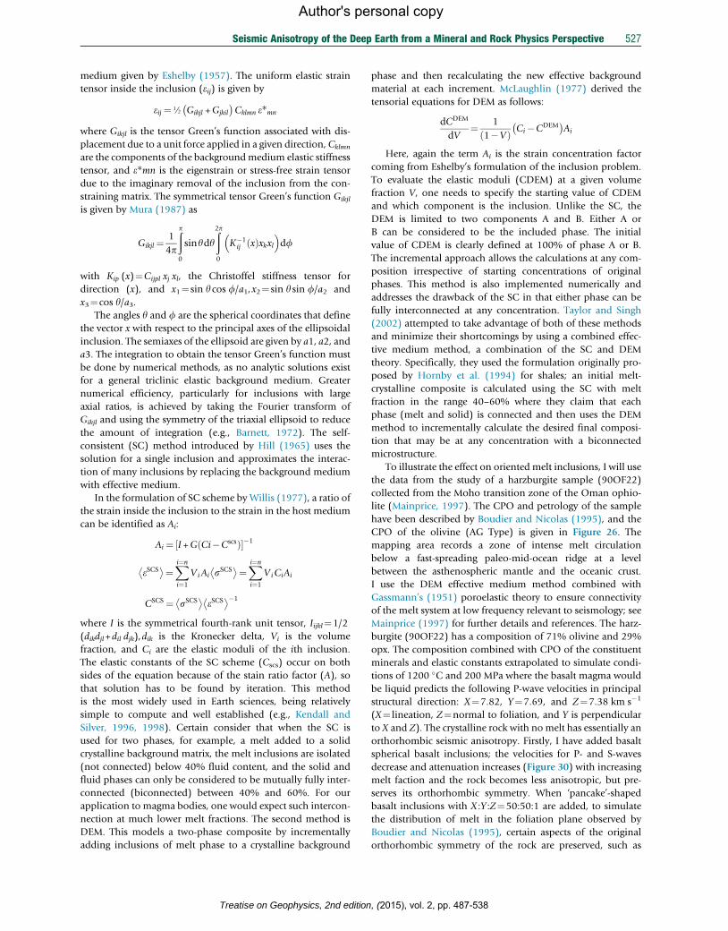
Seismic Anisotropy of the Deep Earth from a Mineral and Rock Physics Perspective 527
Author's personal copy
medium given by Eshelby (1957). The uniform elastic strain
tensor inside the inclusion (eij) is given by
eij ¼ 1⁄2 Gikjl +Gjkil
� �Cklmn e*mn
where Gikjl is the tensor Green’s function associated with dis-
placement due to a unit force applied in a given direction, Cklmn
are the components of the backgroundmedium elastic stiffness
tensor, and e*mn is the eigenstrain or stress-free strain tensor
due to the imaginary removal of the inclusion from the con-
straining matrix. The symmetrical tensor Green’s function Gikjl
is given by Mura (1987) as
Gikjl ¼ 1
4p
ðp0
sinydyð2p0
K�1ij xð Þxkxl
�df
with Kip (x)¼Cijpl xj xl, the Christoffel stiffness tensor for
direction (x), and x1¼ sin ycos f/a1,x2¼ sin y sin f/a2 and
x3¼cos y/a3.The angles y and f are the spherical coordinates that define
the vector x with respect to the principal axes of the ellipsoidal
inclusion. The semiaxes of the ellipsoid are given by a1, a2, and
a3. The integration to obtain the tensor Green’s function must
be done by numerical methods, as no analytic solutions exist
for a general triclinic elastic background medium. Greater
numerical efficiency, particularly for inclusions with large
axial ratios, is achieved by taking the Fourier transform of
Gikjl and using the symmetry of the triaxial ellipsoid to reduce
the amount of integration (e.g., Barnett, 1972). The self-
consistent (SC) method introduced by Hill (1965) uses the
solution for a single inclusion and approximates the interac-
tion of many inclusions by replacing the background medium
with effective medium.
In the formulation of SC scheme by Willis (1977), a ratio of
the strain inside the inclusion to the strain in the host medium
can be identified as Ai:
Ai ¼ I +G Ci�Cscsð Þ½ �1
eSCS ¼Xi¼n
i¼1
ViAi sSCS ¼Xi¼n
i¼1
ViCiAi
CSCS ¼ sSCS
eSCS �1
where I is the symmetrical fourth-rank unit tensor, Iijkl¼1/2
(dikdjl+dil djk),dik is the Kronecker delta, Vi is the volume
fraction, and Ci are the elastic moduli of the ith inclusion.
The elastic constants of the SC scheme (Cscs) occur on both
sides of the equation because of the stain ratio factor (A), so
that solution has to be found by iteration. This method
is the most widely used in Earth sciences, being relatively
simple to compute and well established (e.g., Kendall and
Silver, 1996, 1998). Certain consider that when the SC is
used for two phases, for example, a melt added to a solid
crystalline background matrix, the melt inclusions are isolated
(not connected) below 40% fluid content, and the solid and
fluid phases can only be considered to be mutually fully inter-
connected (biconnected) between 40% and 60%. For our
application to magma bodies, one would expect such intercon-
nection at much lower melt fractions. The second method is
DEM. This models a two-phase composite by incrementally
adding inclusions of melt phase to a crystalline background
Treatise on Geophysics, 2nd edition
phase and then recalculating the new effective background
material at each increment. McLaughlin (1977) derived the
tensorial equations for DEM as follows:
dCDEM
dV¼ 1
1�Vð Þ Ci�CDEM� �
Ai
Here, again the term Ai is the strain concentration factor
coming from Eshelby’s formulation of the inclusion problem.
To evaluate the elastic moduli (CDEM) at a given volume
fraction V, one needs to specify the starting value of CDEM
and which component is the inclusion. Unlike the SC, the
DEM is limited to two components A and B. Either A or
B can be considered to be the included phase. The initial
value of CDEM is clearly defined at 100% of phase A or B.
The incremental approach allows the calculations at any com-
position irrespective of starting concentrations of original
phases. This method is also implemented numerically and
addresses the drawback of the SC in that either phase can be
fully interconnected at any concentration. Taylor and Singh
(2002) attempted to take advantage of both of these methods
and minimize their shortcomings by using a combined effec-
tive medium method, a combination of the SC and DEM
theory. Specifically, they used the formulation originally pro-
posed by Hornby et al. (1994) for shales; an initial melt-
crystalline composite is calculated using the SC with melt
fraction in the range 40–60% where they claim that each
phase (melt and solid) is connected and then uses the DEM
method to incrementally calculate the desired final composi-
tion that may be at any concentration with a biconnected
microstructure.
To illustrate the effect on oriented melt inclusions, I will use
the data from the study of a harzburgite sample (90OF22)
collected from the Moho transition zone of the Oman ophio-
lite (Mainprice, 1997). The CPO and petrology of the sample
have been described by Boudier and Nicolas (1995), and the
CPO of the olivine (AG Type) is given in Figure 26. The
mapping area records a zone of intense melt circulation
below a fast-spreading paleo-mid-ocean ridge at a level
between the asthenospheric mantle and the oceanic crust.
I use the DEM effective medium method combined with
Gassmann’s (1951) poroelastic theory to ensure connectivity
of the melt system at low frequency relevant to seismology; see
Mainprice (1997) for further details and references. The harz-
burgite (90OF22) has a composition of 71% olivine and 29%
opx. The composition combined with CPO of the constituent
minerals and elastic constants extrapolated to simulate condi-
tions of 1200 �C and 200 MPa where the basalt magma would
be liquid predicts the following P-wave velocities in principal
structural direction: X¼7.82, Y¼7.69, and Z¼7.38 km s�1
(X¼ lineation, Z¼normal to foliation, and Y is perpendicular
to X and Z). The crystalline rock with nomelt has essentially an
orthorhombic seismic anisotropy. Firstly, I have added basalt
spherical basalt inclusions; the velocities for P- and S-waves
decrease and attenuation increases (Figure 30) with increasing
melt faction and the rock becomes less anisotropic, but pre-
serves its orthorhombic symmetry. When ‘pancake’-shaped
basalt inclusions with X :Y :Z¼50:50:1 are added, to simulate
the distribution of melt in the foliation plane observed by
Boudier and Nicolas (1995), certain aspects of the original
orthorhombic symmetry of the rock are preserved, such as
, (2015), vol. 2, pp. 487-538
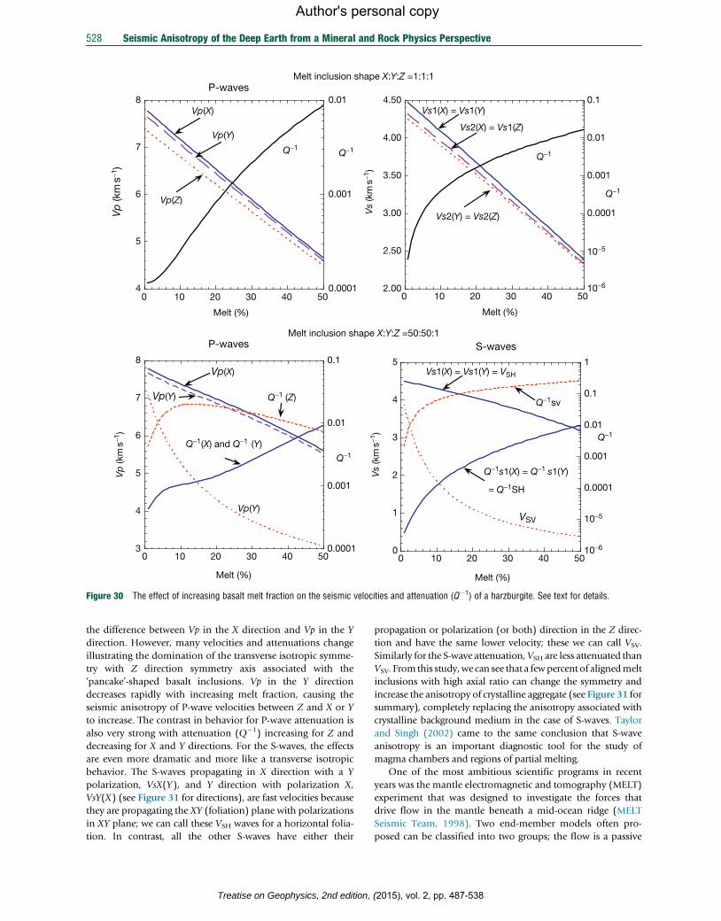
P-waves S-wavesMelt inclusion shape X:Y:Z =50:50:1
P-wavesMelt inclusion shape X:Y:Z =1:1:1
4
5
6
7
8
0.0001
0.001
0.01
0 10 20 30 40 50
Vp
(km
s−1)
Q−1
Q−1
Q−1
Q−1
Melt (%)
Q−1
Vp(X)
Vp(Y)
Vp(Z)
2.00
2.50
3.00
3.50
4.00
4.50
0.0001
0.001
0.01
0.1
0 10 20 30 40 50
Vs
(km
s−1)
Melt (%)
Vs1(X) = Vs1(Y)
Vs2(X) = Vs1(Z)
Vs2(Y) = Vs2(Z)
3
4
5
6
7
8
0.0001
0.001
0.01
0.1
0 10 20 30 40 50
Vp
(km
s−1)
Melt (%)
Vp(X)
Vp(Y)
Vp(Y)
(X) and Q−1 (Y)
(Z)
0
1
2
3
4
5
10−6
10−5
10−6
10−5
0.0001
0.001
0.01
0.1
1
0 10 20 30 40 50
Vs
(km
s−1)
Melt (%)
Vs1(X) = Vs1(Y) = VSH
VSV
s1(X) = Q−1 s1(Y)
= Q−1SH
svQ−1
Q−1
Q−1
Q−1
Q−1
Figure 30 The effect of increasing basalt melt fraction on the seismic velocities and attenuation (Q�1) of a harzburgite. See text for details.
528 Seismic Anisotropy of the Deep Earth from a Mineral and Rock Physics Perspective
Author's personal copy
the difference between Vp in the X direction and Vp in the Y
direction. However, many velocities and attenuations change
illustrating the domination of the transverse isotropic symme-
try with Z direction symmetry axis associated with the
‘pancake’-shaped basalt inclusions. Vp in the Y direction
decreases rapidly with increasing melt fraction, causing the
seismic anisotropy of P-wave velocities between Z and X or Y
to increase. The contrast in behavior for P-wave attenuation is
also very strong with attenuation (Q�1) increasing for Z and
decreasing for X and Y directions. For the S-waves, the effects
are even more dramatic and more like a transverse isotropic
behavior. The S-waves propagating in X direction with a Y
polarization, VsX(Y), and Y direction with polarization X,
VsY(X) (see Figure 31 for directions), are fast velocities because
they are propagating the XY (foliation) plane with polarizations
in XY plane; we can call these VSH waves for a horizontal folia-
tion. In contrast, all the other S-waves have either their
Treatise on Geophysics, 2nd edition,
propagation or polarization (or both) direction in the Z direc-
tion and have the same lower velocity; these we can call VSV.
Similarly for the S-wave attenuation,VSH are less attenuated than
VSV. From this study,we can see that a fewpercent of alignedmelt
inclusions with high axial ratio can change the symmetry and
increase the anisotropy of crystalline aggregate (see Figure 31 for
summary), completely replacing the anisotropy associated with
crystalline background medium in the case of S-waves. Taylor
and Singh (2002) came to the same conclusion that S-wave
anisotropy is an important diagnostic tool for the study of
magma chambers and regions of partial melting.
One of the most ambitious scientific programs in recent
years was the mantle electromagnetic and tomography (MELT)
experiment that was designed to investigate the forces that
drive flow in the mantle beneath a mid-ocean ridge (MELT
Seismic Team, 1998). Two end-member models often pro-
posed can be classified into two groups; the flow is a passive
(2015), vol. 2, pp. 487-538
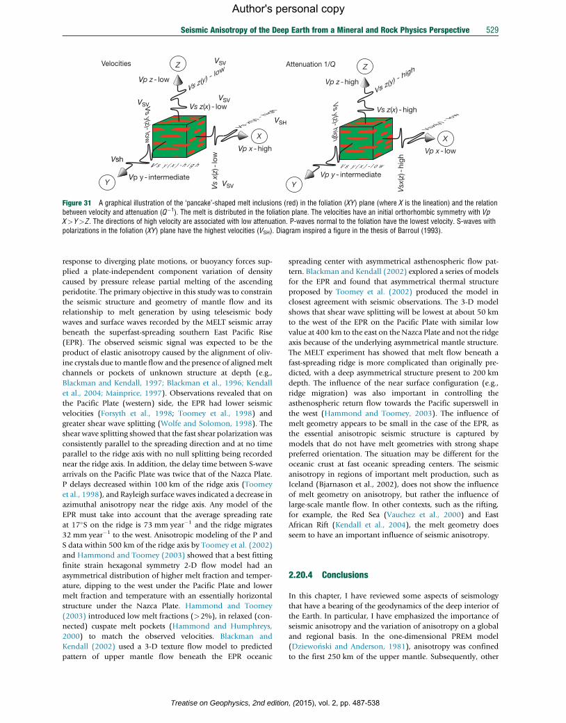
Y
X
Z
Vp x - high
Vp z - low
Vp y - intermediate
Vs z(x) - low
Vs
x(z)
-low
V s y ( x ) - h i g h
Vs y(z)- low
Vs x(y) - high
Vs z(y) -
lowVelocities
VSH
Vsh
VSV
VSV
VSVVSV
Y
X
Z
Vp x - low
Vp z - high
Vp y - intermediate
Vs z(x) - high
Vsx
(z)-
high
V s y ( x ) - l o w
Vs y(z)- high
Vsx(y) - low
Vs z(y) - high
Attenuation 1/Q
Figure 31 A graphical illustration of the ‘pancake’-shaped melt inclusions (red) in the foliation (XY) plane (where X is the lineation) and the relationbetween velocity and attenuation (Q�1). The melt is distributed in the foliation plane. The velocities have an initial orthorhombic symmetry with VpX>Y>Z. The directions of high velocity are associated with low attenuation. P-waves normal to the foliation have the lowest velocity. S-waves withpolarizations in the foliation (XY) plane have the highest velocities (VSH). Diagram inspired a figure in the thesis of Barroul (1993).
Seismic Anisotropy of the Deep Earth from a Mineral and Rock Physics Perspective 529
Author's personal copy
response to diverging plate motions, or buoyancy forces sup-
plied a plate-independent component variation of density
caused by pressure release partial melting of the ascending
peridotite. The primary objective in this study was to constrain
the seismic structure and geometry of mantle flow and its
relationship to melt generation by using teleseismic body
waves and surface waves recorded by the MELT seismic array
beneath the superfast-spreading southern East Pacific Rise
(EPR). The observed seismic signal was expected to be the
product of elastic anisotropy caused by the alignment of oliv-
ine crystals due tomantle flow and the presence of alignedmelt
channels or pockets of unknown structure at depth (e.g.,
Blackman and Kendall, 1997; Blackman et al., 1996; Kendall
et al., 2004; Mainprice, 1997). Observations revealed that on
the Pacific Plate (western) side, the EPR had lower seismic
velocities (Forsyth et al., 1998; Toomey et al., 1998) and
greater shear wave splitting (Wolfe and Solomon, 1998). The
shear wave splitting showed that the fast shear polarization was
consistently parallel to the spreading direction and at no time
parallel to the ridge axis with no null splitting being recorded
near the ridge axis. In addition, the delay time between S-wave
arrivals on the Pacific Plate was twice that of the Nazca Plate.
P delays decreased within 100 km of the ridge axis (Toomey
et al., 1998), and Rayleigh surface waves indicated a decrease in
azimuthal anisotropy near the ridge axis. Any model of the
EPR must take into account that the average spreading rate
at 17�S on the ridge is 73 mm year�1 and the ridge migrates
32 mm year�1 to the west. Anisotropic modeling of the P and
S data within 500 km of the ridge axis by Toomey et al. (2002)
and Hammond and Toomey (2003) showed that a best fitting
finite strain hexagonal symmetry 2-D flow model had an
asymmetrical distribution of higher melt fraction and temper-
ature, dipping to the west under the Pacific Plate and lower
melt fraction and temperature with an essentially horizontal
structure under the Nazca Plate. Hammond and Toomey
(2003) introduced low melt fractions (>2%), in relaxed (con-
nected) cuspate melt pockets (Hammond and Humphreys,
2000) to match the observed velocities. Blackman and
Kendall (2002) used a 3-D texture flow model to predicted
pattern of upper mantle flow beneath the EPR oceanic
Treatise on Geophysics, 2nd edition
spreading center with asymmetrical asthenospheric flow pat-
tern. Blackman and Kendall (2002) explored a series of models
for the EPR and found that asymmetrical thermal structure
proposed by Toomey et al. (2002) produced the model in
closest agreement with seismic observations. The 3-D model
shows that shear wave splitting will be lowest at about 50 km
to the west of the EPR on the Pacific Plate with similar low
value at 400 km to the east on the Nazca Plate and not the ridge
axis because of the underlying asymmetrical mantle structure.
The MELT experiment has showed that melt flow beneath a
fast-spreading ridge is more complicated than originally pre-
dicted, with a deep asymmetrical structure present to 200 km
depth. The influence of the near surface configuration (e.g.,
ridge migration) was also important in controlling the
asthenospheric return flow towards the Pacific superswell in
the west (Hammond and Toomey, 2003). The influence of
melt geometry appears to be small in the case of the EPR, as
the essential anisotropic seismic structure is captured by
models that do not have melt geometries with strong shape
preferred orientation. The situation may be different for the
oceanic crust at fast oceanic spreading centers. The seismic
anisotropy in regions of important melt production, such as
Iceland (Bjarnason et al., 2002), does not show the influence
of melt geometry on anisotropy, but rather the influence of
large-scale mantle flow. In other contexts, such as the rifting,
for example, the Red Sea (Vauchez et al., 2000) and East
African Rift (Kendall et al., 2004), the melt geometry does
seem to have an important influence of seismic anisotropy.
2.20.4 Conclusions
In this chapter, I have reviewed some aspects of seismology
that have a bearing of the geodynamics of the deep interior of
the Earth. In particular, I have emphasized the importance of
seismic anisotropy and the variation of anisotropy on a global
and regional basis. In the one-dimensional PREM model
(Dziewo�nski and Anderson, 1981), anisotropy was confined
to the first 250 km of the upper mantle. Subsequently, other
, (2015), vol. 2, pp. 487-538
530 Seismic Anisotropy of the Deep Earth from a Mineral and Rock Physics Perspective
Author's personal copy
studies of the mantle found various additional forms of global
anisotropy associated with the transition zone, the 670 km
boundary layer, and the D00 layer (e.g., Montagner, 1994a,b;
Montagner and Kennett, 1996; Montagner, 1998). The most
recent global studies using more complete data sets and new
methods of analysis emphasize the exceptionally strong nature
of the upper mantle anisotropy, the anisotropy of the D00 layer,and no significant deviation from the original isotropic PREM
for the rest of the mantle (e.g., Beghein et al., 2006; Panning
and Romanowicz, 2006). To explain velocity variations that
are observed in the mantle studies using probabilistic tomog-
raphy places the emphasis on chemical heterogeneity and
lateral temperature variations in the mantle (Deschamps and
Trampert, 2003; Trampert et al., 2004). Trampert and van der
Hilst (2005) argued that spatial variations in bulk major ele-
ment composition dominate buoyancy in the lowermost man-
tle, but even at shallower depths, its contribution to buoyancy
is comparable to thermal effects. The case of the D00 layer isperhaps even more challenging, as it is clearly a region with not
only strong temperature and compositional gradients (e.g., Lay
et al., 2004) but also a regionally varying seismic anisotropy
(e.g., Maupin et al., 2005; van der Hilst et al., 2007; Wookey
et al., 2005a) with an overall global signature (e.g., Beghein
et al., 2006; Montagner and Kennett, 1996; Panning and
Romanowicz, 2006). The inner core has well-known travel
time variations that can be modeled to fit various single or
double concentric layered anisotropy scenarios. Some studies
(Beghein and Trampert, 2003; Ishii and Dziewo�nski, 2002)
tend to favor a difference in anisotropy between the outermost
inner core and innermost inner core; however, they disagree in
the magnitude and symmetry of the anisotropy. Calvet et al.
(2006) suggested that the data set is too poor to distinguish
between several of the current models, whereas new high-
quality data (Lythgoe et al., 2014) clearly favor a strongly
anisotropic western hemisphere and weakly anisotropic east-
ern one. Lythgoe et al. (2014) also questioned if the outermost
and innermost inner core model is an artifact of not taking into
account the hemispherical structure of the inner core. In the
mantle and the inner core, there are often differences between
studies at the global and regional scales and differences
between 1-D and 3-D global models. The seismic sampling
over different radial and lateral length scales using surface
and body waves of variable frequency has made reference
models very important in the reporting and understanding of
complex data sets. Kennett (2006) had shown, for example, it
is difficult to achieve comparable P- and S-wave definition for
the whole mantle. Mineral physics can play important role as a
representation based on elastic moduli rather than wave speeds
that would provide a better comparator for interpretation in
terms of composition, temperature, and anisotropy.
In addressing the basics of elasticity, wave propagation in
anisotropic crystals, and the nature of the anisotropy polycrys-
talline aggregates with CPO, I hope I have provided some of
keys necessary for the interpretation of seismic anisotropy.
CPO produced by plastic deformation is the link between
deformation history and the seismic anisotropy of the Earth’s
deep interior. We have seen earlier that many regions of the
mantle (e.g., lower mantle) do not have a pronounced seismic
anisotropy. However, from mineral physics, we have seen that
in the upper mantle, olivine has a strong elastic anisotropy; in
Treatise on Geophysics, 2nd edition,
the transition zone, wadsleyite is quite anisotropic; in the
lower mantle, Mg-perovskite and MgO have increasing anisot-
ropy with depth; in the D00 layer, postperovskite is very
anisotropic; and the inner core, hcp iron is moderately aniso-
tropic. In addition, if we add minerals from the hydrated
mantle in subduction regions, such as the antigorite, chlorite,
talc, and brucite, they can be very anisotropic at low pressure
and S-wave anisotropy and can be very high for antigorite and
chlorite even at high pressure. Subduction-related nonhydrous
minerals, such as Al-CF phase, hollandite I, and stishovite, can
have exceptionally high anisotropy in the transition zone and
lower mantle. Potentially, the mineralogy suggests that seismic
anisotropy could be present if these minerals have a CPO.
Aligned melt inclusions and compositional layers can also
produce anisotropy. To understand why there are regions in
the deep Earth that have no seismic anisotropy is clearly a
challenge for mineral physics, seismology, and geodynamics.
Acknowledgments
I thank Guilhem Barruol, Francois Boudier, Patrick Cordier,
Brian Kennett, Bob Liebermann, Katsuyoshi Michibayashi,
Sebastien Merkel, Adolphe Nicolas, Andrea Tommasi, and the
late Paul Silver for their helpful discussions. I thank Don Issak
for providing a copy of his 2001 publication on Elastic Properties
of Minerals and Planetary Objects, which is an excellent compli-
ment to this work. I also thank Steve Jacobsen for providing
preprints of his work on hydrous minerals. I thank Mainak
Mookherjee for providing data in digital format from his publi-
cations. I thank James Wookey for his constructive review of the
first version of this chapter and useful suggestions.
Finally, I thank volume editors G. David Price and Lars
Stixrude for providing the occasion to write this chapter and
both them and series editor Gerald Schubert for their patience
during long gestation of this manuscript.
I dedicate this chapter to the memory of Paul G. Silver,
extraordinary seismologist, genial colleague, and great friend.
References
Abramson EH, Brown JM, Slutsky LJ, and Zaug J (1997) The elastic constants of SanCarlos olivine to 17 GPa. Journal of Geophysical Research 102: 12,253–12,263.
Adams BL, Wright SL, and Kunze K (1993) Orientation mapping: The emergence of anew microscopy. Metallurgical Transactions A 24: 819–831.
Alboussiere T, Deguen R, and Melzani M (2010) Melting-induced stratification abovethe Earth’s inner core due to convective translation. Nature 466: 744–747.
Anderson DL (1979) Deep structure of the continents. Journal of Geophysical Research84: 7555–7560.
Anderson OL and Isaak DG (1995) Elastic constants of mantle minerals at hightemperature. In: Ahrens TJ (ed.) Handbook of Physical Constants, pp. 64–97.Washington, DC: American Geophysical Union.
Andrault D, Fiquet G, Guyot F, and Hanfland M (1998) Pressure induced Landau-typetransition in stishovite. Science 282: 720–724. http://dx.doi.org/10.1126/science.282.5389.720.
Andrault D, Fiquet G, Kunz M, Visocekas F, and Hausermann D (1997) Theorthorhombic structure of iron: An in situ study at high temperature and highpressure. Science 278: 831–834.
Antonangeli D, Komabayashi T, Occelli F, et al. (2012) Simultaneous sound velocity anddensity measurements of hcp iron up to 93 GPa and K: An experimental test of theBirch’s law at high temperature. Earth and Planetary Science Letters331–332: 210–214.
(2015), vol. 2, pp. 487-538
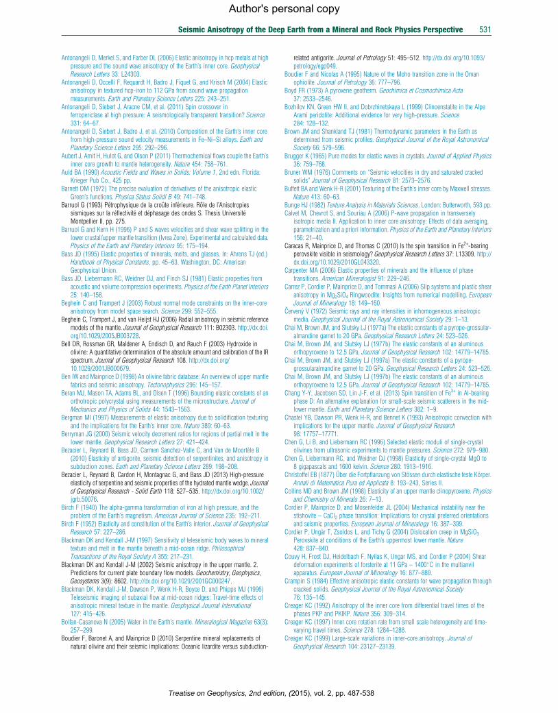
Seismic Anisotropy of the Deep Earth from a Mineral and Rock Physics Perspective 531
Author's personal copy
Antonangeli D, Merkel S, and Farber DL (2006) Elastic anisotropy in hcp metals at highpressure and the sound wave anisotropy of the Earth’s inner core. GeophysicalResearch Letters 33: L24303.
Antonangeli D, Occelli F, Requardt H, Badro J, Fiquet G, and Krisch M (2004) Elasticanisotropy in textured hcp-iron to 112 GPa from sound wave propagationmeasurements. Earth and Planetary Science Letters 225: 243–251.
Antonangeli D, Siebert J, Aracne CM, et al. (2011) Spin crossover inferropericlase at high pressure: A seismologically transparent transition? Science331: 64–67.
Antonangeli D, Siebert J, Badro J, et al. (2010) Composition of the Earth’s inner corefrom high-pressure sound velocity measurements in Fe–Ni–Si alloys. Earth andPlanetary Science Letters 295: 292–296.
Aubert J, Amit H, Hulot G, and Olson P (2011) Thermochemical flows couple the Earth’sinner core growth to mantle heterogeneity. Nature 454: 758–761.
Auld BA (1990) Acoustic Fields and Waves in Solids: Volume 1, 2nd edn. Florida:Krieger Pub Co., 425 pp.
Barnett DM (1972) The precise evaluation of derivatives of the anisotropic elasticGreen’s functions. Physica Status Solidi B 49: 741–748.
Barruol G (1993) Petrophysique de la croute inferieure. Role de l’Anisotropiessismiques sur la reflectivite et dephasage des ondes S. Thesis UniversiteMontpellier II, pp. 275.
Barruol G and Kern H (1996) P and S waves velocities and shear wave splitting in thelower crustal/upper mantle transition (Ivrea Zone). Experimental and calculated data.Physics of the Earth and Planetary Interiors 95: 175–194.
Bass JD (1995) Elastic properties of minerals, melts, and glasses. In: Ahrens TJ (ed.)Handbook of Physical Constants, pp. 45–63. Washington, DC: AmericanGeophysical Union.
Bass JD, Liebermann RC, Weidner DJ, and Finch SJ (1981) Elastic properties fromacoustic and volume compression experiments. Physics of the Earth Planet Interiors25: 140–158.
Beghein C and Trampert J (2003) Robust normal mode constraints on the inner-coreanisotropy from model space search. Science 299: 552–555.
Beghein C, Trampert J, and van Heijst HJ (2006) Radial anisotropy in seismic referencemodels of the mantle. Journal of Geophysical Research 111: B02303. http://dx.doi.org/10.1029/2005JB003728.
Bell DR, Rossman GR, Maldener A, Endisch D, and Rauch F (2003) Hydroxide inolivine: A quantitative determination of the absolute amount and calibration of the IRspectrum. Journal of Geophysical Research 108. http://dx.doi.org/10.1029/2001JB000679.
Ben IW and Mainprice D (1998) An olivine fabric database: An overview of upper mantlefabrics and seismic anisotropy. Tectonophysics 296: 145–157.
Beran MJ, Mason TA, Adams BL, and Olsen T (1996) Bounding elastic constants of anorthotropic polycrystal using measurements of the microstructure. Journal ofMechanics and Physics of Solids 44: 1543–1563.
Bergman MI (1997) Measurements of elastic anisotropy due to solidification texturingand the implications for the Earth’s inner core. Nature 389: 60–63.
Berryman JG (2000) Seismic velocity decrement ratios for regions of partial melt in thelower mantle. Geophysical Research Letters 27: 421–424.
Bezacier L, Reynard B, Bass JD, Carmen Sanchez-Valle C, and Van de Moortele B(2010) Elasticity of antigorite, seismic detection of serpentinites, and anisotropy insubduction zones. Earth and Planetary Science Letters 289: 198–208.
Bezacier L, Reynard B, Cardon H, Montagnac G, and Bass JD (2013) High-pressureelasticity of serpentine and seismic properties of the hydrated mantle wedge. Journalof Geophysical Research - Solid Earth 118: 527–535. http://dx.doi.org/10.1002/jgrb.50076.
Birch F (1940) The alpha-gamma transformation of iron at high pressure, and theproblem of the Earth’s magnetism. American Journal of Science 235: 192–211.
Birch F (1952) Elasticity and constitution of the Earth’s interior. Journal of GeophysicalResearch 57: 227–286.
Blackman DK and Kendall J-M (1997) Sensitivity of teleseismic body waves to mineraltexture and melt in the mantle beneath a mid-ocean ridge. PhilosophicalTransactions of the Royal Society A 355: 217–231.
Blackman DK and Kendall J-M (2002) Seismic anisotropy in the upper mantle. 2.Predictions for current plate boundary flow models. Geochemistry, Geophysics,Geosystems 3(9): 8602. http://dx.doi.org/10.1029/2001GC000247.
Blackman DK, Kendall J-M, Dawson P, Wenk H-R, Boyce D, and Phipps MJ (1996)Teleseismic imaging of subaxial flow at mid-ocean ridges: Travel-time effects ofanisotropic mineral texture in the mantle. Geophysical Journal International127: 415–426.
Bolfan-Casanova N (2005) Water in the Earth’s mantle. Mineralogical Magazine 63(3):257–299.
Boudier F, Baronet A, and Mainprice D (2010) Serpentine mineral replacements ofnatural olivine and their seismic implications: Oceanic lizardite versus subduction-
Treatise on Geophysics, 2nd edition
related antigorite. Journal of Petrology 51: 495–512. http://dx.doi.org/10.1093/petrology/egp049.
Boudier F and Nicolas A (1995) Nature of the Moho transition zone in the Omanophiolite. Journal of Petrology 36: 777–796.
Boyd FR (1973) A pyroxene geotherm. Geochimica et Cosmochimica Acta37: 2533–2546.
Bozhilov KN, Green HW II, and Dobrzhinetskaya L (1999) Clinoenstatite in the AlpeArami peridotite: Additional evidence for very high-pressure. Science284: 128–132.
Brown JM and Shankland TJ (1981) Thermodynamic parameters in the Earth asdetermined from seismic profiles. Geophysical Journal of the Royal AstronomicalSociety 66: 579–596.
Brugger K (1965) Pure modes for elastic waves in crystals. Journal of Applied Physics36: 759–768.
Bruner WM (1976) Comments on “Seismic velocities in dry and saturated crackedsolids” Journal of Geophysical Research 81: 2573–2576.
Buffett BA and Wenk H-R (2001) Texturing of the Earth’s inner core by Maxwell stresses.Nature 413: 60–63.
Bunge HJ (1982) Texture Analysis in Materials Sciences. London: Butterworth, 593 pp.Calvet M, Chevrot S, and Souriau A (2006) P-wave propagation in transversely
isotropic media II. Application to inner core anisotropy: Effects of data averaging,parametrization and a priori information. Physics of the Earth and Planetary Interiors156: 21–40.
Caracas R, Mainprice D, and Thomas C (2010) Is the spin transition in Fe2+-bearingperovskite visible in seismology? Geophysical Research Letters 37: L13309. http://dx.doi.org/10.1029/2010GL043320.
Carpenter MA (2006) Elastic properties of minerals and the influence of phasetransitions. American Mineralogist 91: 229–246.
Carrez P, Cordier P, Mainprice D, and Tommasi A (2006) Slip systems and plastic shearanisotropy in Mg2SiO4 Ringwoodite: Insights from numerical modelling. EuropeanJournal of Mineralogy 18: 149–160.
Cerveny V (1972) Seismic rays and ray intensities in inhomogeneous anisotropicmedia. Geophysical Journal of the Royal Astronomical Society 29: 1–13.
Chai M, Brown JM, and Slutsky LJ (1977a) The elastic constants of a pyrope-grossular-almandine garnet to 20 GPa. Geophysical Research Letters 24: 523–526.
Chai M, Brown JM, and Slutsky LJ (1977b) The elastic constants of an aluminousorthopyroxene to 12.5 GPa. Journal of Geophysical Research 102: 14779–14785.
Chai M, Brown JM, and Slutsky LJ (1997a) The elastic constants of a pyrope-grossularalmandine garnet to 20 GPa. Geophysical Research Letters 24: 523–526.
Chai M, Brown JM, and Slutsky LJ (1997b) The elastic constants of an aluminousorthopyroxene to 12.5 GPa. Journal of Geophysical Research 102: 14779–14785.
Chang Y-Y, Jacobsen SD, Lin J-F, et al. (2013) Spin transition of Fe3+ in Al-bearingphase D: An alternative explanation for small-scale seismic scatterers in the mid-lower mantle. Earth and Planetary Science Letters 382: 1–9.
Chastel YB, Dawson PR, Wenk H-R, and Bennet K (1993) Anisotropic convection withimplications for the upper mantle. Journal of Geophysical Research98: 17757–17771.
Chen G, Li B, and Liebermann RC (1996) Selected elastic moduli of single-crystalolivines from ultrasonic experiments to mantle pressures. Science 272: 979–980.
Chen G, Liebermann RC, and Weidner DJ (1998) Elasticity of single-crystal MgO to8 gigapascals and 1600 kelvin. Science 280: 1913–1916.
Christoffel EB (1877) Uber die Fortpflanzung von St€ossen durch elastische feste K€orper.Annali di Matematica Pura ed Applicata 8: 193–243, Series II.
Collins MD and Brown JM (1998) Elasticity of an upper mantle clinopyroxene. Physicsand Chemistry of Minerals 26: 7–13.
Cordier P, Mainprice D, and Mosenfelder JL (2004) Mechanical instability near thestishovite – CaCl2 phase transition: Implications for crystal preferred orientationsand seismic properties. European Journal of Mineralogy 16: 387–399.
Cordier P, Ungar T, Zsoldos L, and Tichy G (2004) Dislocation creep in MgSiO3Perovskite at conditions of the Earth’s uppermost lower mantle. Nature428: 837–840.
Couvy H, Frost DJ, Heidelbach F, Nyilas K, Ungar MS, and Cordier P (2004) Sheardeformation experiments of forsterite at 11 GPa – 1400�C in the multianvilapparatus. European Journal of Mineralogy 16: 877–889.
Crampin S (1984) Effective anisotropic elastic constants for wave propagation throughcracked solids. Geophysical Journal of the Royal Astronomical Society76: 135–145.
Creager KC (1992) Anisotropy of the inner core from differential travel times of thephases PKP and PKIKP. Nature 356: 309–314.
Creager KC (1997) Inner core rotation rate from small scale heterogeneity and time-varying travel times. Science 278: 1284–1288.
Creager KC (1999) Large-scale variations in inner-core anisotropy. Journal ofGeophysical Research 104: 23127–23139.
, (2015), vol. 2, pp. 487-538
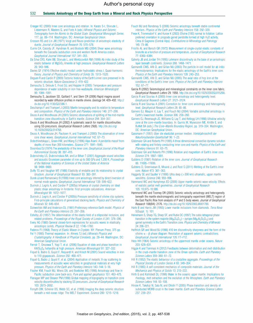
532 Seismic Anisotropy of the Deep Earth from a Mineral and Rock Physics Perspective
Author's personal copy
Creager KC (2000) Inner core anisotropy and rotation. In: Karato S-I, Stixrude L,Liebermann R, Masters G, and Forte A (eds.) Mineral Physics and SeismicTomography from the Atomic to the Global Scale. Geophysical Monograph Series,117, pp. 89–114. Washington, DC: American Geophysical Union.
Crosson RS and Lin JW (1971) Voigt and Reuss prediction of anisotropic elasticity ofdunite. Journal of Geophysical Research 76: 570–578.
Currie CA, Cassidy JF, Hyndman R, and Bostock MG (2004) Shear wave anisotropybeneath the Cascadia subduction zone and western North America craton.Geophysical Journal International 157: 341–353.
Da Silva CRS, Karki BB, Stixrude L, and Wentzcovitch RM (1999) Ab initio study of theelastic behavior of MgSiO3 ilmenite at high pressure. Geophysical Research Letters26: 943–946.
Davies GF (1974) Effective elastic moduli under hydrostatic stress I, Quasi-harmonictheory. Journal of Physics and Chemistry of Solids 35: 1513–1520.
Deguen R and Cardin P (2009) Tectonic history of the Earth’s inner core preserved in itsseismic structure. Nature Geoscience 2: 419–422.
Demouchy S, Deloule E, Frost DJ, and Keppler H (2005) Temperature and pressuredependence of water solubility in iron free-wadsleyite. American Mineralogist90: 1084–1091.
Demouchy S, Jacobsen SD, Gaillard F, and Stern CR (2006) Rapid magma ascentrecorded by water diffusion profiles in mantle olivine. Geology 34: 429–432. http://dx.doi.org/10.1130/G22386.1.
Deschamps F and Trampert J (2003) Mantle tomography and its relation to temperatureand composition. Physics of the Earth and Planetary Interiors 140: 277–299.
Deuss A and Woodhouse JH (2001) Seismic observations of splitting of the mid-mantletransition zone discontinuity in Earth’s mantle. Science 294: 354–357.
Deuss A and Woodhouse JH (2002) A systematic search for mantle discontinuitiesusing SS-precursors. Geophysical Research Letters 29(8). http://dx.doi.org/10.1029/2002GL014768.
Deuss A, Woodhouse JH, Paulssen H, and Trampert J (2000) The observation of innercore shear waves. Geophysical Journal International 142: 67–73.
Dobrzhinetskaya L, Green HW, and Wang S (1996) Alpe Arami: A peridotite massif fromdepths of more than 300 kilometers. Science 271: 1841–1845.
Doornbos DJ (1974) The anelasticity of the inner core. Geophysical Journal of the RoyalAstronomical Society 38: 397–415.
Dubrovinsky LS, Dubrovinskaia NA, and Le Bihan T (2001) Aggregate sound velocitiesand acoustic Gruneisen parameter of iron up to 300 GPa and 1,200 K. Proceedingsof the National Academy of Sciences of the United States of America98: 9484–9489.
Duffy TS and Vaughan MT (1988) Elasticity of enstatite and its relationship to crystalstructure. Journal of Geophysical Research 93: 383–391.
Durek JJ and Romanowicz B (1999) Inner core anisotropy inferred by direct inversion ofnormal mode spectra. Geophysical Journal International 139: 599–622.
Durinck J, Legris A, and Cordier P (2005a) Influence of crystal chemistry on idealplastic shear anisotropy in forsterite: First principle calculations. AmericanMineralogist 90: 1072–1077.
Durinck J, Legris A, and Cordier P (2005b) Pressure sensitivity of olivine slip systems:First-principle calculations of generalised stacking faults. Physics and Chemistry ofMinerals 32: 646–654.
Dziewo�nski AM and Anderson DL (1981) Preliminary reference Earth model. Physics ofthe Earth and Planetary Interiors 25: 297–356.
Eshelby JD (1957) The determination of the elastic field of a ellipsoidal inclusion, andrelated problems. Proceedings of the Royal Society of London A 241: 376–396.
Every AG (1980) General closed-form expressions for acoustic waves in elasticallyanisotropic solids. Physical Review B 22: 1746–1760.
Federov FI (1968) Theory of Elastic Waves in Crystals. NY: Plenum Press, 375 pp.Fei Y (1995) Thermal expansion. In: Ahrens TJ (ed.) Minerals Physics and
Crystallography: A Handbook of Physical Constants, pp. 29–44. Washington, DC:American Geophysical Union.
Ferroir T, Onozawa T, Yagi T, et al. (2006) Equation of state and phase transition inKAlSi3O8 hollandite at high pressure. American Mineralogist 91: 327–332.
Fiquet G, Badro G, Guyot F, Requardt H, and Krisch M (2001) Sound velocities in ironto 110 gigapascals. Science 292: 468–471.
Fiquet G, Badro J, Guyot F, et al. (2004) Application of inelastic X-ray scattering tomeasurements of acoustic wave velocities in geophysical materials at very highpressure. Physics of the Earth and Planetary Interiors 143–144: 5–18.
Fischer KM, Fouch MJ, Wiens DA, and Boettcher MS (1998) Anisotropy and flow inPacific subduction zone back-arcs. Pure and applied geophysics 151: 463–475.
Flanagan MP and Shearer PM (1998) Global mapping of topography on transition zonevelocity discontinuities by stacking SS precursors. Journal of Geophysical Research103: 2673–2692.
Forsyth DW, Scheirer DS, Webb SC, et al. (1998) Imaging the deep seismic structurebeneath a mid-ocean ridge: The MELT Experiment. Science 280: 1215–1218.
Treatise on Geophysics, 2nd edition,
Fouch MJ and Rondenay S (2006) Seismic anisotropy beneath stable continentalinteriors. Physics of the Earth and Planetary Interiors 158: 292–320.
Frese K, Trommsdorf V, and Kunze K (2003) Olivine [100] normal to foliation: Latticepreferred orientation in prograde garnet peridotite formed at high H2O activity,Cima di Gagnone (Central Alps). Contributions to Mineralogy and Petrology145: 73–86.
Frisillo AL and Barsch GR (1972) Measurement of single-crystal elastic constants ofbronzite as a function of pressure and temperature. Journal of Geophysical Research77: 6360–6384.
Gaherty JB and Jordan TH (1995) Lehmann discontinuity as the base of an anisotropiclayer beneath continents. Science 268: 1468–1471.
Gannarelli CMS, Alfe D, and Gillan MJ (2003) The particle-in-cell model for ab initiothermodynamics: Implications for the elastic anisotropy of the Earth’s inner core.Physics of the Earth and Planetary Interiors 139: 243–253.
Gannarelli CMS, Alfe D, and Gillan MJ (2005) The axial ratio of hcp iron at theconditions of the Earth’s inner core. Physics of the Earth and Planetary Interiors152: 67–77.
Garcia R (2002) Seismological and mineralogical constraints on the inner core fabric.Geophysical Research Letters 29: 1958. http://dx.doi.org/10.1029/2002GL015268.
Garcia R and Souriau A (2000) Inner core anisotropy and heterogeneity level.Geophysical Research Letters 27: 3121–3124.
Garcia R and Souriau A (2001) Correction to: Inner core anisotropy and heterogeneitylevel. Geophysical Research Letters 28: 85–86.
Garnero EJ, Maupin V, Lay T, and Fouch MJ (2004) Variable azimuthal anisotropy inEarth’s lowermost mantle. Science 306: 259–260.
Garnero EJ, Revenaugh JS, Williams Q, Lay T, and Kellogg LH (1998) Ultralow velocityzone at the core–mantle boundary. In: Gurnis M, Wysession ME, Knittle E, andBuffett BA (eds.) The Core–Mantle Boundary Region, pp. 319–334. Washington,DC: American Geophysical Union.
Gassmann F (1951) Uber die elastizitat poroser medien. Vierteljahrsschrift derNaturforschenden Gesellschaft 96: 1–23.
Glatzmaier GA and Roberts PH (1995) A three dimensional convective dynamo solutionwith rotating and finitely conducting inner core and mantle. Physics of the Earth andPlanetary Interiors 91: 63–75.
Glatzmaier GA and Roberts PH (1996) Rotation and magnetism of Earth’s inner core.Science 274: 1887–1891.
Gubbins D (1981) Rotation of the inner core. Journal of Geophysical Research86: 11695–11699.
Gubbins D, Sreenivasan B, Mound J, and Rost S (2011) Melting of the Earth’s innercore. Nature 473: 361–363.
Haggerty SE and Sautter V (1990) Ultra deep (>300 km) ultramafic, upper mantlexenoliths. Science 248: 993–996.
Hammond WC and Humphreys ED (2000) Upper mantle seismic wave velocity: Effectsof realistic partial melt geometries. Journal of Geophysical Research105: 10,975–10,986.
Hammond WC and Toomey DR (2003) Seismic velocity anisotropy and heterogeneitybeneath the mantle electromagnetic and tomography experiment (MELT) region ofthe East Pacific Rise from analysis of P and S body waves. Journal of GeophysicalResearch 108(B4): 2176. http://dx.doi.org/10.1029/2002JB001789.
Harte B and Harris JW (1993) Lower mantle inclusions from diamonds. Terra Nova5(Suppl. 1): 101.
Heinemann S, Sharp TG, Sharp SF, and Rubie DC (1997) The cubic-tetragonal phasetransition in the system majorite (Mg4Si4O12) – pyrope (Mg3Al2Si3O12) andgarnet symmetry in the Earth’s Transition zone. Physics and Chemistry of Minerals24: 206–221.
Helffrich GR and Wood BJ (1996) 410 km discontinuity sharpness and the form of theolivine a�b phase diagram: Resolution of apparent seismic contradictions.Geophysical Journal International 126: F7–F12.
Hess HH (1964) Seismic anisotropy of the uppermost mantle under oceans. Nature203: 629–631.
Higgie K and Tommasi A (2012) Feedbacks between deformation and melt distributionin the crust–mantle transition zone of the Oman ophiolite. Earth and PlanetaryScience Letters 359–360: 61–72.
Hill R (1952) The elastic behaviour of a crystalline aggregate. Proceedings of thePhysical Society of London Series A 65: 349–354.
Hill R (1965) A self consistent mechanics of composite materials. Journal of theMechanics and Physics of Solids 13: 213–222.
Hirth G and Kohlstedt DL (1996) Water in the oceanic upper mantle: Implications forrheology, melt extraction and the evolution of the lithosphere. Earth and PlanetaryScience Letters 144: 93–108.
Hirose K, Takafuji N, Sata N, and Ohishi Y (2005) Phase transition and density ofsubducted MORB crust in the lower mantle. Earth and Planetary Science Letters237: 239–251.
(2015), vol. 2, pp. 487-538
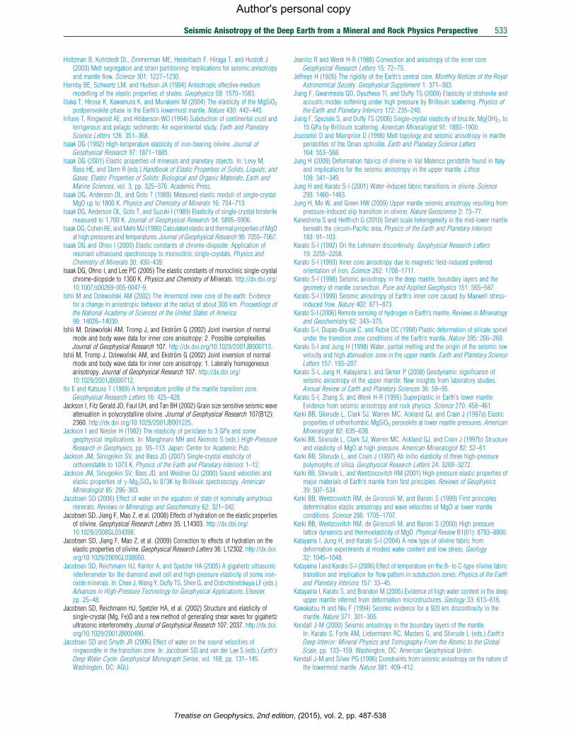
Seismic Anisotropy of the Deep Earth from a Mineral and Rock Physics Perspective 533
Author's personal copy
Holtzman B, Kohlstedt DL, Zimmerman ME, Heidelbach F, Hiraga T, and Hustoft J(2003) Melt segregation and strain partitioning: Implications for seismic anisotropyand mantle flow. Science 301: 1227–1230.
Hornby BE, Schwartz LM, and Hudson JA (1994) Anisotropic effective-mediummodelling of the elastic properties of shales. Geophysics 59: 1570–1583.
Iitaka T, Hirose K, Kawamura K, and Murakami M (2004) The elasticity of the MgSiO3postperovskite phase in the Earth’s lowermost mantle. Nature 430: 442–445.
Irifune T, Ringwood AE, and Hibberson WO (1994) Subduction of continental crust andterrigenous and pelagic sediments: An experimental study. Earth and PlanetaryScience Letters 126: 351–368.
Isaak DG (1992) High-temperature elasticity of iron-bearing olivine. Journal ofGeophysical Research 97: 1871–1885.
Isaak DG (2001) Elastic properties of minerals and planetary objects. In: Levy M,Bass HE, and Stern R (eds.) Handbook of Elastic Properties of Solids, Liquids, andGases. Elastic Properties of Solids: Biological and Organic Materials, Earth andMarine Sciences, vol. 3, pp. 325–376. Academic Press.
Isaak DG, Anderson OL, and Goto T (1989) Measured elastic moduli of single-crystalMgO up to 1800 K. Physics and Chemistry of Minerals 16: 704–713.
Isaak DG, Anderson OL, Goto T, and Suzuki I (1989) Elasticity of single-crystal forsteritemeasured to 1,700 K. Journal of Geophysical Research 94: 5895–5906.
Isaak DG, Cohen RE, andMehl MJ (1990) Calculated elastic and thermal properties of MgOat high pressures and temperatures. Journal of Geophysical Research 95: 7055–7067.
Isaak DG and Ohno I (2003) Elastic constants of chrome-diopside: Application ofresonant ultrasound spectroscopy to monoclinic single-crystals. Physics andChemistry of Minerals 30: 430–439.
Isaak DG, Ohno I, and Lee PC (2005) The elastic constants of monoclinic single-crystalchrome-diopside to 1300 K. Physics and Chemistry of Minerals. http://dx.doi.org/10.1007/s00269-005-0047-9.
Ishii M and Dziewo�nski AM (2002) The innermost inner core of the earth: Evidencefor a change in anisotropic behavior at the radius of about 300 km. Proceedings ofthe National Academy of Sciences of the United States of America99: 14026–14030.
Ishii M, Dziewo�nski AM, Tromp J, and Ekstr€om G (2002) Joint inversion of normalmode and body wave data for inner core anisotropy: 2. Possible complexities.Journal of Geophysical Research 107. http://dx.doi.org/10.1029/2001JB000713.
Ishii M, Tromp J, Dziewo�nski AM, and Ekstr€om G (2002) Joint inversion of normalmode and body wave data for inner core anisotropy: 1. Laterally homogeneousanisotropy. Journal of Geophysical Research 107. http://dx.doi.org/10.1029/2001JB000712.
Ito E and Katsura T (1989) A temperature profile of the mantle transition zone.Geophysical Research Letters 16: 425–428.
Jackson I, Fitz Gerald JD, Faul UH, and Tan BH (2002) Grain size sensitive seismic waveattenuation in polycrystalline olivine. Journal of Geophysical Research 107(B12):2360. http://dx.doi.org/10.1029/2001JB001225.
Jackson I and Niesler H (1982) The elasticity of periclase to 3 GPa and somegeophysical implications. In: Manghnani MH and Akimoto S (eds.) High-PressureResearch in Geophysics, pp. 93–113. Japan: Center for Academic Pub.
Jackson JM, Sinogeikin SV, and Bass JD (2007) Single-crystal elasticity oforthoenstatite to 1073 K. Physics of the Earth and Planetary Interiors 1–12.
Jackson JM, Sinogeikin SV, Bass JD, and Weidner DJ (2000) Sound velocities andelastic properties of g-Mg2SiO4 to 873K by Brillouin spectroscopy. AmericanMineralogist 85: 296–303.
Jacobsen SD (2006) Effect of water on the equation of state of nominally anhydrousminerals. Reviews in Mineralogy and Geochemistry 62: 321–342.
Jacobsen SD, Jiang F, Mao Z, et al. (2008) Effects of hydration on the elastic propertiesof olivine. Geophysical Research Letters 35: L14303. http://dx.doi.org/10.1029/2008GL034398.
Jacobsen SD, Jiang F, Mao Z, et al. (2009) Correction to effects of hydration on theelastic properties of olivine. Geophysical Research Letters 36: L12302. http://dx.doi.org/10.1029/2009GL038660.
Jacobsen SD, Reichmann HJ, Kantor A, and Spetzler HA (2005) A gigahertz ultrasonicinterferometer for the diamond anvil cell and high-pressure elasticity of some iron-oxide minerals. In: Chen J, Wang Y, Duffy TS, Shen G, and Dobrzhinetskaya LF (eds.)Advances in High-Pressure Technology for Geophysical Applications, Elsevier,pp. 25–48.
Jacobsen SD, Reichmann HJ, Spetzler HA, et al. (2002) Structure and elasticity ofsingle-crystal (Mg, Fe)O and a new method of generating shear waves for gigahertzultrasonic interferometry. Journal of Geophysical Research 107: 2037. http://dx.doi.org/10.1029/2001JB000490.
Jacobsen SD and Smyth JR (2006) Effect of water on the sound velocities ofringwoodite in the transition zone. In: Jacobsen SD and van der Lee S (eds.) Earth’sDeep Water Cycle. Geophysical Monograph Series, vol. 168, pp. 131–145.Washington, DC: AGU.
Treatise on Geophysics, 2nd edition
Jeanloz R and Wenk H-R (1988) Convection and anisotropy of the inner core.Geophysical Research Letters 15: 72–75.
Jeffreys H (1926) The rigidity of the Earth’s central core. Monthly Notices of the RoyalAstronomical Society. Geophysical Supplement 1: 371–383.
Jiang F, Gwanmesia GD, Dyuzheva TI, and Duffy TS (2009) Elasticity of stishovite andacoustic modes softening under high pressure by Brillouin scattering. Physics ofthe Earth and Planetary Interiors 172: 235–240.
Jiang F, Speziale S, and Duffy TS (2006) Single-crystal elasticity of brucite, Mg(OH)2, to15 GPa by Brillouin scattering. American Mineralogist 91: 1893–1900.
Jousselin D and Mainprice D (1998) Melt topology and seismic anisotropy in mantleperidotites of the Oman ophiolite. Earth and Planetary Science Letters164: 553–568.
Jung H (2009) Deformation fabrics of olivine in Val Malenco peridotite found in Italyand implications for the seismic anisotropy in the upper mantle. Lithos109: 341–349.
Jung H and Karato S-I (2001) Water-induced fabric transitions in olivine. Science293: 1460–1463.
Jung H, Mo W, and Green HW (2009) Upper mantle seismic anisotropy resulting frompressure-induced slip transition in olivine. Nature Geoscience 2: 73–77.
Kaneshima S and Helffrich G (2010) Small scale heterogeneity in the mid-lower mantlebeneath the circum-Pacific area. Physics of the Earth and Planetary Interiors183: 91–103.
Karato S-I (1992) On the Lehmann discontinuity. Geophysical Research Letters19: 2255–2258.
Karato S-I (1993) Inner core anisotropy due to magnetic field-induced preferredorientation of iron. Science 262: 1708–1711.
Karato S-I (1998) Seismic anisotropy in the deep mantle, boundary layers and thegeometry of mantle convection. Pure and Applied Geophysics 151: 565–587.
Karato S-I (1999) Seismic anisotropy of Earth’s inner core caused by Maxwell stress-induced flow. Nature 402: 871–873.
Karato S-I (2006) Remote sensing of hydrogen in Earth’s mantle. Reviews in Mineralogyand Geochemistry 62: 343–375.
Karato S-I, Dupas-Bruzek C, and Rubie DC (1998) Plastic deformation of silicate spinelunder the transition zone conditions of the Earth’s mantle. Nature 395: 266–269.
Karato S-I and Jung H (1998) Water, partial melting and the origin of the seismic lowvelocity and high attenuation zone in the upper mantle. Earth and Planetary ScienceLetters 157: 193–207.
Karato S-I, Jung H, Katayama I, and Skmer P (2008) Geodynamic significance ofseismic anisotropy of the upper mantle: New insights from laboratory studies.Annual Review of Earth and Planetary Sciences 36: 59–95.
Karato S-I, Zhang S, and Wenk H-R (1995) Superplastic in Earth’s lower mantle:Evidence from seismic anisotropy and rock physics. Science 270: 458–461.
Karki BB, Stixrude L, Clark SJ, Warren MC, Ackland GJ, and Crain J (1997a) Elasticproperties of orthorhombic MgSiO3 perovskite at lower mantle pressures. AmericanMineralogist 82: 635–638.
Karki BB, Stixrude L, Clark SJ, Warren MC, Ackland GJ, and Crain J (1997b) Structureand elasticity of MgO at high pressure. American Mineralogist 82: 52–61.
Karki BB, Stixrude L, and Crain J (1997) Ab initio elasticity of three high-pressurepolymorphs of silica. Geophysical Research Letters 24: 3269–3272.
Karki BB, Stixrude L, and Wentzocovitch RM (2001) High-pressure elastic properties ofmajor materials of Earth’s mantle from first principles. Reviews of Geophysics39: 507–534.
Karki BB, Wentzcovitch RM, de Gironcoli M, and Baroni S (1999) First principlesdetermination elastic anisotropy and wave velocities of MgO at lower mantleconditions. Science 286: 1705–1707.
Karki BB, Wentzcovitch RM, de Gironcoli M, and Baroni S (2000) High pressurelattice dynamics and thermoelasticity of MgO. Physical Review B1(61): 8793–8800.
Katayama I, Jung H, and Karato S-I (2004) A new type of olivine fabric fromdeformation experiments at modest water content and low stress. Geology32: 1045–1048.
Katayama I and Karato S-I (2006) Effect of temperature on the B- to C-type olivine fabrictransition and implication for flow pattern in subduction zones. Physics of the Earthand Planetary Interiors 157: 33–45.
Katayama I, Karato S, and Brandon M (2005) Evidence of high water content in the deepupper mantle inferred from deformation microstructures. Geology 33: 613–616.
Kawakatsu H and Niu F (1994) Seismic evidence for a 920 km discontinuity in themantle. Nature 371: 301–305.
Kendall J-M (2000) Seismic anisotropy in the boundary layers of the mantle.In: Karato S, Forte AM, Liebermann RC, Masters G, and Stixrude L (eds.) Earth’sDeep Interior: Mineral Physics and Tomography From the Atomic to the GlobalScale, pp. 133–159. Washington, DC: American Geophysical Union.
Kendall J-M and Silver PG (1996) Constraints from seismic anisotropy on the nature ofthe lowermost mantle. Nature 381: 409–412.
, (2015), vol. 2, pp. 487-538
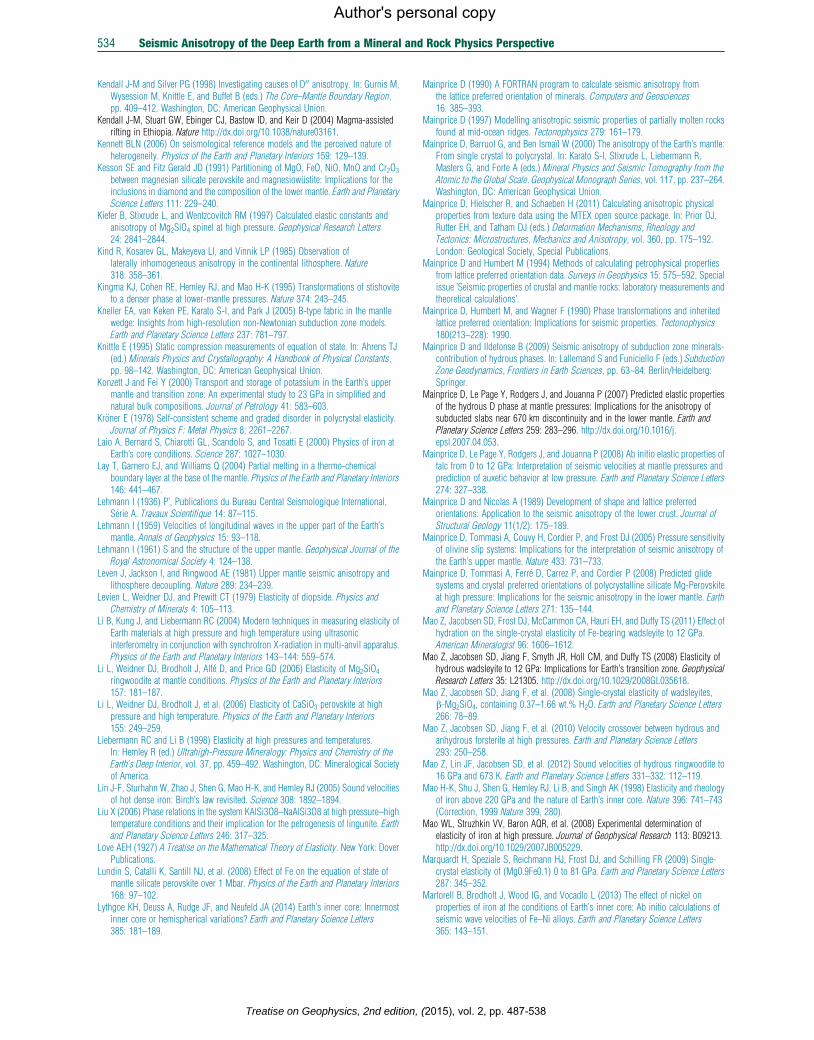
534 Seismic Anisotropy of the Deep Earth from a Mineral and Rock Physics Perspective
Author's personal copy
Kendall J-M and Silver PG (1998) Investigating causes of D00 anisotropy. In: Gurnis M,Wysession M, Knittle E, and Buffet B (eds.) The Core–Mantle Boundary Region,pp. 409–412. Washington, DC: American Geophysical Union.
Kendall J-M, Stuart GW, Ebinger CJ, Bastow ID, and Keir D (2004) Magma-assistedrifting in Ethiopia. Nature http://dx.doi.org/10.1038/nature03161.
Kennett BLN (2006) On seismological reference models and the perceived nature ofheterogeneity. Physics of the Earth and Planetary Interiors 159: 129–139.
Kesson SE and Fitz Gerald JD (1991) Partitioning of MgO, FeO, NiO, MnO and Cr2O3between magnesian silicate perovskite and magnesiowustite: Implications for theinclusions in diamond and the composition of the lower mantle. Earth and PlanetaryScience Letters 111: 229–240.
Kiefer B, Stixrude L, and Wentzcovitch RM (1997) Calculated elastic constants andanisotropy of Mg2SiO4 spinel at high pressure. Geophysical Research Letters24: 2841–2844.
Kind R, Kosarev GL, Makeyeva LI, and Vinnik LP (1985) Observation oflaterally inhomogeneous anisotropy in the continental lithosphere. Nature318: 358–361.
Kingma KJ, Cohen RE, Hemley RJ, and Mao H-K (1995) Transformations of stishoviteto a denser phase at lower-mantle pressures. Nature 374: 243–245.
Kneller EA, van Keken PE, Karato S-I, and Park J (2005) B-type fabric in the mantlewedge: Insights from high-resolution non-Newtonian subduction zone models.Earth and Planetary Science Letters 237: 781–797.
Knittle E (1995) Static compression measurements of equation of state. In: Ahrens TJ(ed.) Minerals Physics and Crystallography: A Handbook of Physical Constants,pp. 98–142. Washington, DC: American Geophysical Union.
Konzett J and Fei Y (2000) Transport and storage of potassium in the Earth’s uppermantle and transition zone: An experimental study to 23 GPa in simplified andnatural bulk compositions. Journal of Petrology 41: 583–603.
Kr€oner E (1978) Self-consistent scheme and graded disorder in polycrystal elasticity.Journal of Physics F: Metal Physics 8: 2261–2267.
Laio A, Bernard S, Chiarotti GL, Scandolo S, and Tosatti E (2000) Physics of iron atEarth’s core conditions. Science 287: 1027–1030.
Lay T, Garnero EJ, and Williams Q (2004) Partial melting in a thermo-chemicalboundary layer at the base of the mantle. Physics of the Earth and Planetary Interiors146: 441–467.
Lehmann I (1936) P’, Publications du Bureau Central Seismologique International,Serie A. Travaux Scientifique 14: 87–115.
Lehmann I (1959) Velocities of longitudinal waves in the upper part of the Earth’smantle. Annals of Geophysics 15: 93–118.
Lehmann I (1961) S and the structure of the upper mantle. Geophysical Journal of theRoyal Astronomical Society 4: 124–138.
Leven J, Jackson I, and Ringwood AE (1981) Upper mantle seismic anisotropy andlithosphere decoupling. Nature 289: 234–239.
Levien L, Weidner DJ, and Prewitt CT (1979) Elasticity of diopside. Physics andChemistry of Minerals 4: 105–113.
Li B, Kung J, and Liebermann RC (2004) Modern techniques in measuring elasticity ofEarth materials at high pressure and high temperature using ultrasonicinterferometry in conjunction with synchrotron X-radiation in multi-anvil apparatus.Physics of the Earth and Planetary Interiors 143–144: 559–574.
Li L, Weidner DJ, Brodholt J, Alfe D, and Price GD (2006) Elasticity of Mg2SiO4ringwoodite at mantle conditions. Physics of the Earth and Planetary Interiors157: 181–187.
Li L, Weidner DJ, Brodholt J, et al. (2006) Elasticity of CaSiO3 perovskite at highpressure and high temperature. Physics of the Earth and Planetary Interiors155: 249–259.
Liebermann RC and Li B (1998) Elasticity at high pressures and temperatures.In: Hemley R (ed.) Ultrahigh-Pressure Mineralogy: Physics and Chemistry of theEarth’s Deep Interior, vol. 37, pp. 459–492. Washington, DC: Mineralogical Societyof America.
Lin J-F, Sturhahn W, Zhao J, Shen G, Mao H-K, and Hemley RJ (2005) Sound velocitiesof hot dense iron: Birch’s law revisited. Science 308: 1892–1894.
Liu X (2006) Phase relations in the system KAlSi3O8–NaAlSi3O8 at high pressure–hightemperature conditions and their implication for the petrogenesis of lingunite. Earthand Planetary Science Letters 246: 317–325.
Love AEH (1927) A Treatise on the Mathematical Theory of Elasticity. New York: DoverPublications.
Lundin S, Catalli K, Santill NJ, et al. (2008) Effect of Fe on the equation of state ofmantle silicate perovskite over 1 Mbar. Physics of the Earth and Planetary Interiors168: 97–102.
Lythgoe KH, Deuss A, Rudge JF, and Neufeld JA (2014) Earth’s inner core: Innermostinner core or hemispherical variations? Earth and Planetary Science Letters385: 181–189.
Treatise on Geophysics, 2nd edition,
Mainprice D (1990) A FORTRAN program to calculate seismic anisotropy fromthe lattice preferred orientation of minerals. Computers and Geosciences16: 385–393.
Mainprice D (1997) Modelling anisotropic seismic properties of partially molten rocksfound at mid-ocean ridges. Tectonophysics 279: 161–179.
Mainprice D, Barruol G, and Ben Ismaıl W (2000) The anisotropy of the Earth’s mantle:From single crystal to polycrystal. In: Karato S-I, Stixrude L, Liebermann R,Masters G, and Forte A (eds.) Mineral Physics and Seismic Tomography from theAtomic to the Global Scale. Geophysical Monograph Series, vol. 117, pp. 237–264.Washington, DC: American Geophysical Union.
Mainprice D, Hielscher R, and Schaeben H (2011) Calculating anisotropic physicalproperties from texture data using the MTEX open source package. In: Prior DJ,Rutter EH, and Tatham DJ (eds.) Deformation Mechanisms, Rheology andTectonics: Microstructures, Mechanics and Anisotropy, vol. 360, pp. 175–192.London: Geological Society, Special Publications.
Mainprice D and Humbert M (1994) Methods of calculating petrophysical propertiesfrom lattice preferred orientation data. Surveys in Geophysics 15: 575–592, Specialissue ’Seismic properties of crustal and mantle rocks: laboratory measurements andtheoretical calculations’.
Mainprice D, Humbert M, and Wagner F (1990) Phase transformations and inheritedlattice preferred orientation: Implications for seismic properties. Tectonophysics180(213–228): 1990.
Mainprice D and Ildefonse B (2009) Seismic anisotropy of subduction zone minerals-contribution of hydrous phases. In: Lallemand S and Funiciello F (eds.) SubductionZone Geodynamics, Frontiers in Earth Sciences, pp. 63–84. Berlin/Heidelberg:Springer.
Mainprice D, Le Page Y, Rodgers J, and Jouanna P (2007) Predicted elastic propertiesof the hydrous D phase at mantle pressures: Implications for the anisotropy ofsubducted slabs near 670 km discontinuity and in the lower mantle. Earth andPlanetary Science Letters 259: 283–296. http://dx.doi.org/10.1016/j.epsl.2007.04.053.
Mainprice D, Le Page Y, Rodgers J, and Jouanna P (2008) Ab initio elastic properties oftalc from 0 to 12 GPa: Interpretation of seismic velocities at mantle pressures andprediction of auxetic behavior at low pressure. Earth and Planetary Science Letters274: 327–338.
Mainprice D and Nicolas A (1989) Development of shape and lattice preferredorientations: Application to the seismic anisotropy of the lower crust. Journal ofStructural Geology 11(1/2): 175–189.
Mainprice D, Tommasi A, Couvy H, Cordier P, and Frost DJ (2005) Pressure sensitivityof olivine slip systems: Implications for the interpretation of seismic anisotropy ofthe Earth’s upper mantle. Nature 433: 731–733.
Mainprice D, Tommasi A, Ferre D, Carrez P, and Cordier P (2008) Predicted glidesystems and crystal preferred orientations of polycrystalline silicate Mg-Perovskiteat high pressure: Implications for the seismic anisotropy in the lower mantle. Earthand Planetary Science Letters 271: 135–144.
Mao Z, Jacobsen SD, Frost DJ, McCammon CA, Hauri EH, and Duffy TS (2011) Effect ofhydration on the single-crystal elasticity of Fe-bearing wadsleyite to 12 GPa.American Mineralogist 96: 1606–1612.
Mao Z, Jacobsen SD, Jiang F, Smyth JR, Holl CM, and Duffy TS (2008) Elasticity ofhydrous wadsleyite to 12 GPa: Implications for Earth’s transition zone. GeophysicalResearch Letters 35: L21305. http://dx.doi.org/10.1029/2008GL035618.
Mao Z, Jacobsen SD, Jiang F, et al. (2008) Single-crystal elasticity of wadsleyites,b-Mg2SiO4, containing 0.37–1.66 wt.% H2O. Earth and Planetary Science Letters266: 78–89.
Mao Z, Jacobsen SD, Jiang F, et al. (2010) Velocity crossover between hydrous andanhydrous forsterite at high pressures. Earth and Planetary Science Letters293: 250–258.
Mao Z, Lin JF, Jacobsen SD, et al. (2012) Sound velocities of hydrous ringwoodite to16 GPa and 673 K. Earth and Planetary Science Letters 331–332: 112–119.
Mao H-K, Shu J, Shen G, Hemley RJ, Li B, and Singh AK (1998) Elasticity and rheologyof iron above 220 GPa and the nature of Earth’s inner core. Nature 396: 741–743(Correction, 1999 Nature 399, 280).
Mao WL, Struzhkin VV, Baron AQR, et al. (2008) Experimental determination ofelasticity of iron at high pressure. Journal of Geophysical Research 113: B09213.http://dx.doi.org/10.1029/2007JB005229.
Marquardt H, Speziale S, Reichmann HJ, Frost DJ, and Schilling FR (2009) Single-crystal elasticity of (Mg0.9Fe0.1) 0 to 81 GPa. Earth and Planetary Science Letters287: 345–352.
Martorell B, Brodholt J, Wood IG, and Vocadlo L (2013) The effect of nickel onproperties of iron at the conditions of Earth’s inner core: Ab initio calculations ofseismic wave velocities of Fe–Ni alloys. Earth and Planetary Science Letters365: 143–151.
(2015), vol. 2, pp. 487-538
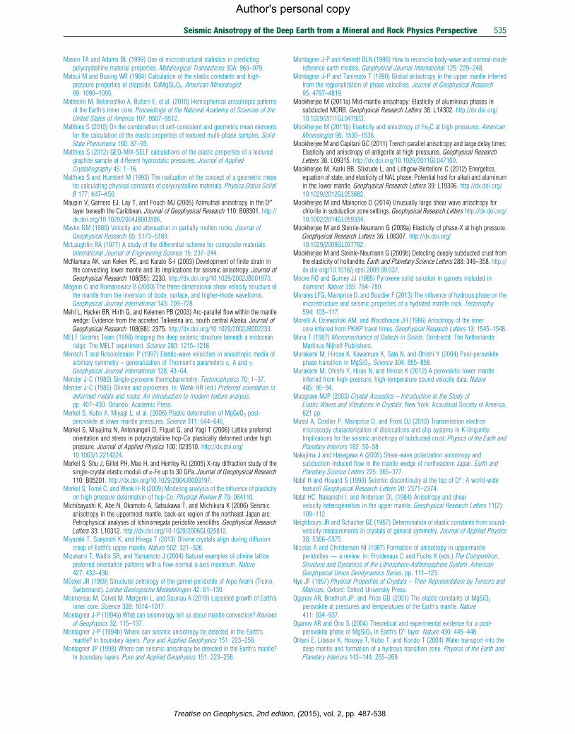
Seismic Anisotropy of the Deep Earth from a Mineral and Rock Physics Perspective 535
Author's personal copy
Mason TA and Adams BL (1999) Use of microstructural statistics in predictingpolycrystalline material properties. Metallurgical Transactions 30A: 969–979.
Matsui M and Busing WR (1984) Calculation of the elastic constants and high-pressure properties of diopside, CaMgSi2O6. American Mineralogist69: 1090–1095.
Mattesini M, Belonoshko A, Buforn E, et al. (2010) Hemispherical anisotropic patternsof the Earth’s inner core. Proceedings of the National Academy of Sciences of theUnited States of America 107: 9507–9512.
Matthies S (2010) On the combination of self-consistent and geometric mean elementsfor the calculation of the elastic properties of textured multi-phase samples. SolidState Phenomena 160: 87–93.
Matthies S (2012) GEO-MIX-SELF calculations of the elastic properties of a texturedgraphite sample at different hydrostatic pressures. Journal of AppliedCrystallography 45: 1–16.
Matthies S and Humbert M (1993) The realization of the concept of a geometric meanfor calculating physical constants of polycrystalline materials. Physica Status SolidiB 177: K47–K50.
Maupin V, Garnero EJ, Lay T, and Fouch MJ (2005) Azimuthal anisotropy in the D00
layer beneath the Caribbean. Journal of Geophysical Research 110: B08301. http://dx.doi.org/10.1029/2004JB003506.
Mavko GM (1980) Velocity and attenuation in partially molten rocks. Journal ofGeophysical Research 85: 5173–5189.
McLaughlin RA (1977) A study of the differential scheme for composite materials.International Journal of Engineering Science 15: 237–244.
McNamara AK, van Keken PE, and Karato S-I (2003) Development of finite strain inthe convecting lower mantle and its implications for seismic anisotropy. Journal ofGeophysical Research 108(B5): 2230. http://dx.doi.org/10.1029/2002JB001970.
Megnin C and Romanowicz B (2000) The three-dimensional shear velocity structure ofthe mantle from the inversion of body, surface, and higher-mode waveforms.Geophysical Journal International 143: 709–728.
Mehl L, Hacker BR, Hirth G, and Kelemen PB (2003) Arc-parallel flow within the mantlewedge: Evidence from the accreted Talkeetna arc, south central Alaska. Journal ofGeophysical Research 108(B8): 2375. http://dx.doi.org/10.1029/2002JB002233.
MELT Seismic Team (1998) Imaging the deep seismic structure beneath a midoceanridge: The MELT experiment. Science 280: 1215–1218.
Mensch T and Rosolofosaon P (1997) Elastic-wave velocities in anisotropic media ofarbitrary symmetry – generalization of Thomsen’s parameters e, d and g.Geophysical Journal International 128: 43–64.
Mercier J-C (1980) Single-pyroxene thermobarometry. Tectonophysics 70: 1–37.Mercier J-C (1985) Olivine and pyroxenes. In: Wenk HR (ed.) Preferred orientation in
deformed metals and rocks: An introduction to modern texture analysis,pp. 407–430. Orlando: Academic Press.
Merkel S, Kubo A, Miyagi L, et al. (2006) Plastic deformation of MgGeO3 post-perovskite at lower mantle pressures. Science 311: 644–646.
Merkel S, Miyajima N, Antonangeli D, Fiquet G, and Yagi T (2006) Lattice preferredorientation and stress in polycrystalline hcp-Co plastically deformed under highpressure. Journal of Applied Physics 100: 023510. http://dx.doi.org/10.1063/1.2214224.
Merkel S, Shu J, Gillet PH, Mao H, and Hemley RJ (2005) X-ray diffraction study of thesingle-crystal elastic moduli of e-Fe up to 30 GPa. Journal of Geophysical Research110: B05201. http://dx.doi.org/10.1029/2004JB003197.
Merkel S, Tome C, and Wenk H-R (2009) Modeling analysis of the influence of plasticityon high pressure deformation of hcp-Co. Physical Review B 79: 064110.
Michibayashi K, Abe N, Okamoto A, Satsukawa T, and Michikura K (2006) Seismicanisotropy in the uppermost mantle, back-arc region of the northeast Japan arc:Petrophysical analyses of Ichinomegata peridotite xenoliths. Geophysical ResearchLetters 33: L10312. http://dx.doi.org/10.1029/2006GL025812.
Miyazaki T, Sueyoshi K, and Hiraga T (2013) Olivine crystals align during diffusioncreep of Earth’s upper mantle. Nature 502: 321–326.
Mizukami T, Wallis SR, and Yamamoto J (2004) Natural examples of olivine latticepreferred orientation patterns with a flow-normal a-axis maximum. Nature427: 432–436.
M€ockel JR (1969) Structural petrology of the garnet-peridotite of Alpe Arami (Ticino,Switzerland). Leidse Geologische Mededelingen 42: 61–130.
Monnereau M, Calvet M, Margerin L, and Souriau A (2010) Lopsided growth of Earth’sinner core. Science 328: 1014–1017.
Montagner J-P (1994a) What can seismology tell us about mantle convection? Reviewsof Geophysics 32: 115–137.
Montagner J-P (1994b) Where can seismic anisotropy be detected in the Earth’smantle? In boundary layers. Pure and Applied Geophysics 151: 223–256.
Montagner JP (1998) Where can seismic anisotropy be detected in the Earth’s mantle?In boundary layers. Pure and Applied Geophysics 151: 223–256.
Treatise on Geophysics, 2nd edition
Montagner J-P and Kennett BLN (1996) How to reconcile body-wave and normal-modereference earth models. Geophysical Journal International 125: 229–248.
Montagner J-P and Tanimoto T (1990) Global anisotropy in the upper mantle inferredfrom the regionalization of phase velocities. Journal of Geophysical Research95: 4797–4819.
Mookherjee M (2011a) Mid-mantle anisotropy: Elasticity of aluminous phases insubducted MORB. Geophysical Research Letters 38: L14302. http://dx.doi.org/10.1029/2011GL047923.
Mookherjee M (2011b) Elasticity and anisotropy of Fe3C at high pressures. AmericanMineralogist 96: 1530–1536.
Mookherjee M and Capitani GC (2011) Trench parallel anisotropy and large delay times:Elasticity and anisotropy of antigorite at high pressures. Geophysical ResearchLetters 38: L09315. http://dx.doi.org/10.1029/2011GL047160.
Mookherjee M, Karki BB, Stixrude L, and Lithgow-Bertelloni C (2012) Energetics,equation of state, and elasticity of NAL phase: Potential host for alkali and aluminumin the lower mantle. Geophysical Research Letters 39: L19306. http://dx.doi.org/10.1029/2012GL053682.
Mookherjee M and Mainprice D (2014) Unusually large shear wave anisotropy forchlorite in subduction zone settings. Geophysical Research Letters http://dx.doi.org/10.1002/2014GL059334.
Mookherjee M and Steinle-Neumann G (2009a) Elasticity of phase-X at high pressure.Geophysical Research Letters 36: L08307. http://dx.doi.org/10.1029/2009GL037782.
Mookherjee M and Steinle-Neumann G (2009b) Detecting deeply subducted crust fromthe elasticity of hollandite. Earth and Planetary Science Letters 288: 349–358. http://dx.doi.org/10.1016/j.epsl.2009.09.037.
Moore RO and Gurney JJ (1985) Pyroxene solid solution in garnets included indiamond. Nature 335: 784–789.
Morales LFG, Mainprice D, and Boudier F (2013) The influence of hydrous phase on themicrostructure and seismic properties of a hydrated mantle rock. Tectonophy594: 103–117.
Morelli A, Dziewo�nski AM, and Woodhouse JH (1986) Anisotropy of the innercore inferred from PKIKP travel times. Geophysical Research Letters 13: 1545–1548.
Mura T (1987) Micromechanics of Defects in Solids. Dordrecht, The Netherlands:Martinus Nijhoff Publishers.
Murakami M, Hirose K, Kawamura K, Sata N, and Ohishi Y (2004) Post-perovskitephase transition in MgSiO3. Science 304: 855–858.
Murakami M, Ohishi Y, Hirao N, and Hirose K (2012) A perovskitic lower mantleinferred from high-pressure, high-temperature sound velocity data. Nature485: 90–94.
Musgrave MJP (2003) Crystal Acoustics – Introduction to the Study ofElastic Waves and Vibrations in Crystals. New York: Acoustical Society of America,621 pp.
Mussi A, Cordier P, Mainprice D, and Frost DJ (2010) Transmission electronmicroscopy characterization of dislocations and slip systems in K-lingunite:Implications for the seismic anisotropy of subducted crust. Physics of the Earth andPlanetary Interiors 182: 50–58.
Nakajima J and Hasegawa A (2005) Shear-wave polarization anisotropy andsubduction-induced flow in the mantle wedge of northeastern Japan. Earth andPlanetary Science Letters 225: 365–377.
Nataf H and Houard S (1993) Seismic discontinuity at the top of D00 : A world-widefeature? Geophysical Research Letters 20: 2371–2374.
Nataf HC, Nakanishi I, and Anderson DL (1984) Anisotropy and shearvelocity heterogeneities in the upper mantle. Geophysical Research Letters 11(2):109–112.
Neighbours JR and Schacher GE (1967) Determination of elastic constants from sound-velocity measurements in crystals of general symmetry. Journal of Applied Physics38: 5366–5375.
Nicolas A and Christensen NI (1987) Formation of anisotropy in uppermantleperidotites — a review. In: Froidevaux C and Fuchs K (eds.) The Composition,Structure and Dynamics of the Lithosphere-Asthenosphere System, AmericanGeophysical Union Geodynamics Series, pp. 111–123.
Nye JF (1957) Physical Properties of Crystals – Their Representation by Tensors andMatrices. Oxford: Oxford University Press.
Oganov AR, Brodholt JP, and Price GD (2001) The elastic constants of MgSiO3perovskite at pressures and temperatures of the Earth’s mantle. Nature411: 934–937.
Oganov AR and Ono S (2004) Theoretical and experimental evidence for a post-perovskite phase of MgSiO3 in Earth’s D
00 layer. Nature 430: 445–448.Ohtani E, Litasov K, Hosoya T, Kubo T, and Kondo T (2004) Water transport into the
deep mantle and formation of a hydrous transition zone. Physics of the Earth andPlanetary Interiors 143–144: 255–269.
, (2015), vol. 2, pp. 487-538
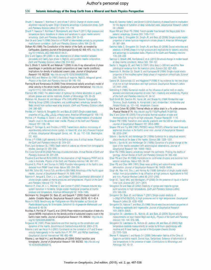
536 Seismic Anisotropy of the Deep Earth from a Mineral and Rock Physics Perspective
Author's personal copy
Ohuchi T, Kawazoe T, Nishihara Y, and Irifune T (2012) Change of olivine a-axisalignment induced by water: Origin of seismic anisotropy in subduction zones. Earthand Planetary Science Letters 317–318: 111–119.
Ohuchi T, Kawazoe T, Nishihara Y, Nishiyama N, and Irifune T (2011) High pressure andtemperature fabric transitions in olivine and variations in upper mantle seismicanisotropy. Earth and Planetary Science Letters 304: 55–63.
Okal EA and Cansi Y (1998) Detection of PKJKP at intermediate periods by progressivemultichannel correlation. Earth and Planetary Science Letters 164: 23–30.
Oldham RD (1906) The Constitution of the Interior of the Earth, as revealed byEarthquakes. Quarterly Journal of the Geological Society 62: 456–475. http://dx.doi.org/10.1144/GSL.JGS.1906.062.01-04.21.
Ono S and Oganov AR (2005) In situ observations of phase transition betweenperovskite and CaIrO3-type phase in MgSiO3 and pyrolitic mantle composition.Earth and Planetary Science Letters 236: 914–932.
Ono S, Ohishi Y, Isshiki M, and Watanuki T (2005) In situ X-ray observations of phaseassemblages in peridotite and basalt compositions at lower mantle conditions:Implications for density of subducted oceanic plate. Journal of GeophysicalResearch 110: B02208. http://dx.doi.org/10.1029/2004JB003196.
Pacalo REG and Weidner DJ (1997) Elasticity of majorite, MgSiO3 tetragonal garnet.Physics of the Earth and Planetary Interiors 99: 145–154.
Panning M and Romanowicz B (2006) Three-dimensional radially anisotropic model ofshear velocity in the whole mantle. Geophysical Journal International. http://dx.doi.org/10.1111/j.1365-246X.2006.03100.x.
Paterson MS (1982) The determination of hydroxyl by infrared absorption in quartz,silicate glasses and similar materials. Bulletin of Mineralogy 105: 20–29.
Pedersen HA, Bruneton M, and Maupin VThe SVKLAPKO Seismic TomographyWorking Group (2006) Lithospheric and sublithospheric anisotropy beneath theBaltic shield from surface-wave array analysis. Earth and Planetary Science Letters244: 590–605.
Perrillat J-P, Fabrizio N, Sinogeikin SV, and Bass JD (2007) Single-crystal elasticproperties of Ca0.07Mg1.93Si2O6 orthopyroxene. American Mineralogist 92: 109–113.
Perrillat J-P, Ricolleau A, Daniel I, et al. (2006) Phase transformations of subductedbasaltic crust in the upmost lower mantle. Physics of the Earth and PlanetaryInteriors 157: 139–149.
Phakey P, Dollinger G, and Christie J (1972) Transmission electron microscopy ofexperimentally deformed olivine crystals. In: Heard HC, et al. (ed.) Flow and Fractureof Rocks. Geophysical Monograph Series, vol. 16, pp. 117–138. Washington,DC: AGU.
Poirier J-P (1994) Light elements in the Earth’s outer core: A critical review. Physics ofthe Earth and Planetary Interiors 85: 319–337.
Polet J and Anderson DL (1995) Depth extent of cratons as inferred from tomographicstudies. Geology 23: 205–208.
Poli S and Schmidt M (2002) Petrology of subducted slabs. Annual Review of Earth andPlanetary Sciences 30: 207–235.
Poupinet G and Kennett BLN (2004) On the observation of high frequency PKiKP and itscoda in Australia. Physics of the Earth and Planetary Interiors 146: 497–511.
Poupinet G, Pillet R, and Souriau A (1983) Possible heterogeneity of the Earth’s corededuced from PKIKP travel times. Nature 305: 204–206.
Raitt RW, Schor GG, Francis TJG, and Morris GB (1969) Anisotropy of the Pacific uppermantle. Journal of Geophysical Research 74: 3095–3109.
Raterron P, Amiguet E, Chen J, Li L, and Cordier P (2009) Experimental deformation ofolivine single crystals at mantle pressures and temperatures. Physics of the Earthand Planetary Interiors 172: 74–83.
Raterron P, Chen JH, Li L, Weidner D, and Cordier P (2007) Pressure-induced slip-system transition in forsterite: Single-crystal rheological properties at mantlepressure and temperature. American Mineralogist 92: 1436–1445.
Reichmann HJ, Sinogeikin SV, Bass JD, and Gasparik T (2002) Elastic moduli ofJadeite- Enstatite Majorite, Geophysical Research Letters 29(19): 42-1–42-4.
Reuss A (1929) Berechnung der Fließgrenze von Mischkristallen auf Grund derPlastizitatsbedingung fur Einkristalle. Zeitschrift fur Angewandte Mathematik undMechanik 9: 49–58.
Ricolleau A, Perrillat JP, Fiquet G, et al. (2010) Phase relations and equation of state of anatural MORB: Implications for the density profile of subducted oceanic crust in theEarth’s lower mantle. Journal of Geophysical Research 115: B08202. http://dx.doi.org/10.1029/2009JB006709.
Ringwood AE (1991) Phase transitions and their bearing on the constitution anddynamics of the mantle. Geochimica et Cosmochimica Acta 55: 2083–2110.
Ritsema J and van Heijst H-J (2001) Constraints on the correlation of P and S-wavevelocity heterogeneity in the mantle from P, PP, PPP, and PKPab traveltimes.Geophysical Journal International 149: 482–489.
Ritsema J, van Heijst H-J, and Woodhouse JH (2004) Global transition zonetomography. Journal of Geophysical Research 109: B02302. http://dx.doi.org/10.1029/2003JB002610.
Treatise on Geophysics, 2nd edition,
Rosa AD, Sanchez-Valle C, and Ghosh S (2012) Elasticity of phase D and its implicationfor the degree of hydration of deep subducted slabs. Geophysical Research Letters39: L06304.
Russo RM and Silver PG (1994) Trench-parallel flow beneath the Nazca plate fromseismic anisotropy. Science 263: 1105–1111.
Sanchez-Valle C, Sinogeikin SV, Smyth JR, and Bass JD (2006) Single-crystal elasticproperties of dense hydrous magnesium silicate phase A. American Mineralogist91: 961–964.
Sanchez-Valle C, Sinogeikin SV, Smyth JR, and Bass JD (2008) Sound velocities andelasticity of DHMS phase A to high pressure and implications for seismic velocitiesand anisotropy in subducted slabs. Physics of the Earth and Planetary Interiors170: 229–239.
Sanloup C, Drewitt JWE, Konopkova Z, et al. (2013) Structural change in molten basaltat deep mantle conditions. Nature 503: 104–107.
Sautter V, Haggerty SE, and Field S (1991) Ultra deep (>300 km) xenoliths: Newpetrological evidence from the transition zone. Science 252: 827–830.
Sawamoto H, Weidner DJ, Sasaki S, and Kumazawa M (1984) Single-crystal elasticproperties of the modified-spinel (beta) phase of magnesium orthosilicate. Science224: 749–751.
Saxena SK, Dubrovinsky LS, and Haggkvist P (1996) X-ray evidence for the new phaseof b-iron at high temperature and high pressure. Geophysical Research Letters23: 2441–2444.
Schmeling H (1985) Numerical models on the influence of partial melt on elastic,anelastic and electrical properties of rocks. Part I: Elasticity and anelasticity. Physicsof the Earth and Planetary Interiors 41: 34–57.
Scott-Smith BH, Danchin RV, Harris JW, and Stracke KJ (1984) Kimberlites nearOrrorroo, South Australia. In: Kornprobst J (ed.) Kimberlites I: Kimberlites andRelated Rocks, pp. 121–142. Amsterdam: Elsevier.
Sha X and Cohen RE (2006) Thermal effects on lattice strain in e-Fe under pressure.Physical Review B 74. http://dx.doi.org/10.1103/PhysRevB.74.064103.
Sha X and Cohen RE (2010) First-principles thermal equation of state andthermoelasticity of hcp Fe at high pressures. Physical Review 81: 1–10.
Shearer PM (1996) Transition zone velocity gradients and the 520 km discontinuity.Journal of Geophysical Research 101: 3053–3066.
Shearer PM and Toy KM (1991) PKP(BC) versus PKP(DF) differential travel times andaspherical structure in the Earth’s inner core. Journal of Geophysical Research96: 2233–2247.
Sidorin I, Gurnis M, and Helmberger DV (1999a) Evidence for a ubiquitous seismicdiscontinuity at the base of the mantle. Science 286: 1326–1331.
Sidorin I, Gurnis M, and Helmberger DV (1999b) Dynamics of a phase change at thebase of the mantle consistent with seismological observations. Journal ofGeophysical Research 104: 15005–15023.
Silver PG (1996) Seismic anisotropy beneath the continents: Probing the depths ofgeology. Annual Review of Earth and Planetary Sciences 24: 385–432.
Silver PG and Chan W (1988) Implications for continental structure and evolution fromseismic anisotropy. Nature 335: 34–39.
Silver PG and Chan WW (1991) Shear wave splitting and subcontinental mantledeformation. Journal of Geophysical Research 96: 16429–16454.
Singh AK, Mao H-K, Shu J, and Hemley RJ (1998) Estimation of single crystal elasticmoduli from polycrystalline X-ray diffraction at high pressure: Applications to FeOand iron. Physical Reviews Letters 80: 2157–2160.
Singh SC, Taylor MAJ, and Montagner J-P (2000) On the presence of liquid in Earth’sinner core. Science 287: 2471–2474.
Sinogeikin SV and Bass JD (2002) Elasticity of pyrope and majorite-pyropesolid solutions to high temperatures. Earth and Planetary Science Letters203: 549–555.
Sinogeikin SV, Bass JD, and Katsura T (2001) Single-crystal elasticity ofg-(Mg0.91Fe0.09)2SiO4 to high pressures and to high temperatures. GeophysicalResearch Letters 28: 4335–4338.
Sinogeikin SV, Katsura T, and Bass JD (1998) Sound velocities and elastic properties ofFe-bearing wadsleyite and ringwoodite. Journal of Geophysical Research103: 20819–20825.
Sinogeikin SV, Lakshtanov DL, Nichola JD, and Bass JD (2004) Sound velocitymeasurements on laser-heated MgO and Al2O3. Physics of the Earth and PlanetaryInteriors 143–144: 575–586.
Sinogeikin SV, Lakshtanov DL, Nichola JD, Jackson JM, and Bass JD (2005) Hightemperature elasticity measurements on oxides by Brillouin spectroscopy withresistive and IR laser heating. Journal of the European Ceramic Society25: 1313–1324.
Skemer P, Katayama I, and Karato S-I (2006) Deformation fabrics of the Cima diGagnone peridotite massif, Central Alps, Switzerland: Evidence of deformation atlow temperatures in the presence of water. Contributions to Mineralogy andPetrology 152: 43–51.
(2015), vol. 2, pp. 487-538
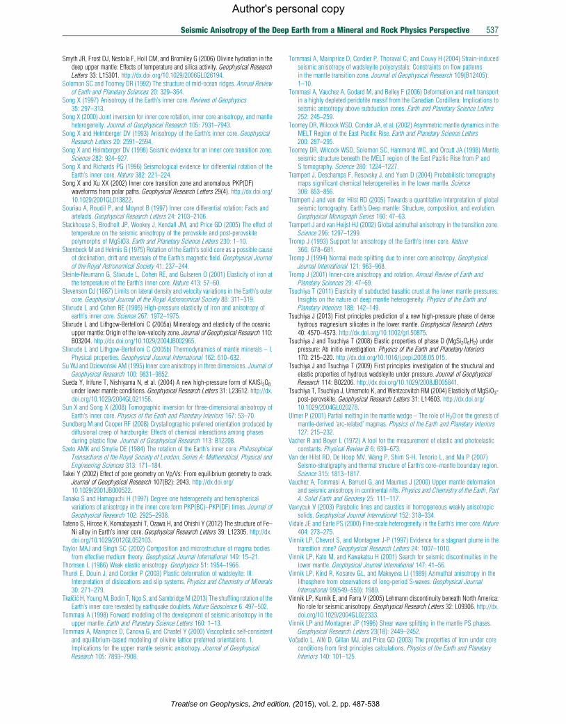
Seismic Anisotropy of the Deep Earth from a Mineral and Rock Physics Perspective 537
Author's personal copy
Smyth JR, Frost DJ, Nestola F, Holl CM, and Bromiley G (2006) Olivine hydration in thedeep upper mantle: Effects of temperature and silica activity. Geophysical ResearchLetters 33: L15301. http://dx.doi.org/10.1029/2006GL026194.
Solomon SC and Toomey DR (1992) The structure of mid-ocean ridges. Annual Reviewof Earth and Planetary Sciences 20: 329–364.
Song X (1997) Anisotropy of the Earth’s inner core. Reviews of Geophysics35: 297–313.
Song X (2000) Joint inversion for inner core rotation, inner core anisotropy, and mantleheterogeneity. Journal of Geophysical Research 105: 7931–7943.
Song X and Helmberger DV (1993) Anisotropy of the Earth’s inner core. GeophysicalResearch Letters 20: 2591–2594.
Song X and Helmberger DV (1998) Seismic evidence for an inner core transition zone.Science 282: 924–927.
Song X and Richards PG (1996) Seismological evidence for differential rotation of theEarth’s inner core. Nature 382: 221–224.
Song X and Xu XX (2002) Inner core transition zone and anomalous PKP(DF)waveforms from polar paths. Geophysical Research Letters 29(4). http://dx.doi.org/10.1029/2001GL013822.
Souriau A, Roudil P, and Moynot B (1997) Inner core differential rotation: Facts andartefacts. Geophysical Research Letters 24: 2103–2106.
Stackhouse S, Brodholt JP, Wookey J, Kendall JM, and Price GD (2005) The effect oftemperature on the seismic anisotropy of the perovskite and post-perovskitepolymorphs of MgSiO3. Earth and Planetary Science Letters 230: 1–10.
Steenbeck M and Helmis G (1975) Rotation of the Earth’s solid core as a possible causeof declination, drift and reversals of the Earth’s magnetic field. Geophysical Journalof the Royal Astronomical Society 41: 237–244.
Steinle-Neumann G, Stixrude L, Cohen RE, and Gulseren O (2001) Elasticity of iron atthe temperature of the Earth’s inner core. Nature 413: 57–60.
Stevenson DJ (1987) Limits on lateral density and velocity variations in the Earth’s outercore. Geophysical Journal of the Royal Astronomical Society 88: 311–319.
Stixrude L and Cohen RE (1995) High-pressure elasticity of iron and anisotropy ofearth’s inner core. Science 267: 1972–1975.
Stixrude L and Lithgow-Bertelloni C (2005a) Mineralogy and elasticity of the oceanicupper mantle: Origin of the low-velocity zone. Journal of Geophysical Research 110:B03204. http://dx.doi.org/10.1029/2004JB002965.
Stixrude L and Lithgow-Bertelloni C (2005b) Thermodynamics of mantle minerals – I.Physical properties. Geophysical Journal International 162: 610–632.
Su WJ and Dziewo�nski AM (1995) Inner core anisotropy in three dimensions. Journal ofGeophysical Research 100: 9831–9852.
Sueda Y, Irifune T, Nishiyama N, et al. (2004) A new high-pressure form of KAlSi3O8under lower mantle conditions. Geophysical Research Letters 31: L23612. http://dx.doi.org/10.1029/2004GL021156.
Sun X and Song X (2008) Tomographic inversion for three-dimensional anisotropy ofEarth’s inner core. Physics of the Earth and Planetary Interiors 167: 53–70.
Sundberg M and Cooper RF (2008) Crystallographic preferred orientation produced bydiffusional creep of harzburgite: Effects of chemical interactions among phasesduring plastic flow. Journal of Geophysical Research 113: B12208.
Szeto AMK and Smylie DE (1984) The rotation of the Earth’s inner core. PhilosophicalTransactions of the Royal Society of London, Series A: Mathematical, Physical andEngineering Sciences 313: 171–184.
Takei Y (2002) Effect of pore geometry on Vp/Vs: From equilibrium geometry to crack.Journal of Geophysical Research 107(B2): 2043. http://dx.doi.org/10.1029/2001JB000522.
Tanaka S and Hamaguchi H (1997) Degree one heterogeneity and hemisphericalvariations of anisotropy in the inner core form PKP(BC)–PKP(DF) times. Journal ofGeophysical Research 102: 2925–2938.
Tateno S, Hirose K, Komabayashi T, Ozawa H, and Ohishi Y (2012) The structure of Fe–Ni alloy in Earth’s inner core. Geophysical Research Letters 39: L12305. http://dx.doi.org/10.1029/2012GL052103.
Taylor MAJ and Singh SC (2002) Composition and microstructure of magma bodiesfrom effective medium theory. Geophysical Journal International 149: 15–21.
Thomsen L (1986) Weak elastic anisotropy. Geophysics 51: 1954–1966.Thurel E, Douin J, and Cordier P (2003) Plastic deformation of wadsleyite: III.
Interpretation of dislocations and slip systems. Physics and Chemistry of Minerals30: 271–279.
Tkalcic H, YoungM, Bodin T, Ngo S, and SambridgeM (2013) The shuffling rotation of theEarth’s inner core revealed by earthquake doublets. Nature Geoscience 6: 497–502.
Tommasi A (1998) Forward modeling of the development of seismic anisotropy in theupper mantle. Earth and Planetary Science Letters 160: 1–13.
Tommasi A, Mainprice D, Canova G, and Chastel Y (2000) Viscoplastic self-consistentand equilibrium-based modeling of olivine lattice preferred orientations. 1.Implications for the upper mantle seismic anisotropy. Journal of GeophysicalResearch 105: 7893–7908.
Treatise on Geophysics, 2nd edition
Tommasi A, Mainprice D, Cordier P, Thoraval C, and Couvy H (2004) Strain-inducedseismic anisotropy of wadsleyite polycrystals: Constraints on flow patternsin the mantle transition zone. Journal of Geophysical Research 109(B12405):1–10.
Tommasi A, Vauchez A, Godard M, and Belley F (2006) Deformation and melt transportin a highly depleted peridotite massif from the Canadian Cordillera: Implications toseismic anisotropy above subduction zones. Earth and Planetary Science Letters252: 245–259.
Toomey DR, Wilcock WSD, Conder JA, et al. (2002) Asymmetric mantle dynamics in theMELT Region of the East Pacific Rise. Earth and Planetary Science Letters200: 287–295.
Toomey DR, Wilcock WSD, Solomon SC, Hammond WC, and Orcutt JA (1998) Mantleseismic structure beneath the MELT region of the East Pacific Rise from P andS tomography. Science 280: 1224–1227.
Trampert J, Deschamps F, Resovsky J, and Yuen D (2004) Probabilistic tomographymaps significant chemical heterogeneities in the lower mantle. Science306: 853–856.
Trampert J and van der Hilst RD (2005) Towards a quantitative interpretation of globalseismic tomography. Earth’s Deep mantle: Structure, composition, and evolution.Geophysical Monograph Series 160: 47–63.
Trampert J and van Heijst HJ (2002) Global azimuthal anisotropy in the transition zone.Science 296: 1297–1299.
Tromp J (1993) Support for anisotropy of the Earth’s inner core. Nature366: 678–681.
Tromp J (1994) Normal mode splitting due to inner core anisotropy. GeophysicalJournal International 121: 963–968.
Tromp J (2001) Inner-core anisotropy and rotation. Annual Review of Earth andPlanetary Sciences 29: 47–69.
Tsuchiya T (2011) Elasticity of subducted basaltic crust at the lower mantle pressures:Insights on the nature of deep mantle heterogeneity. Physics of the Earth andPlanetary Interiors 188: 142–149.
Tsuchiya J (2013) First principles prediction of a new high-pressure phase of densehydrous magnesium silicates in the lower mantle. Geophysical Research Letters40: 4570–4573. http://dx.doi.org/10.1002/grl.50875.
Tsuchiya J and Tsuchiya T (2008) Elastic properties of phase D (MgSi2O6H2) underpressure: Ab initio investigation. Physics of the Earth and Planetary Interiors170: 215–220. http://dx.doi.org/10.1016/j.pepi.2008.05.015.
Tsuchiya J and Tsuchiya T (2009) First principles investigation of the structural andelastic properties of hydrous wadsleyite under pressure. Journal of GeophysicalResearch 114: B02206. http://dx.doi.org/10.1029/2008JB005841.
Tsuchiya T, Tsuchiya J, Umemoto K, and Wentzcovitch RM (2004) Elasticity of MgSiO3-post-perovskite. Geophysical Research Letters 31: L14603. http://dx.doi.org/10.1029/2004GL020278.
Ulmer P (2001) Partial melting in the mantle wedge – The role of H2O on the genesis ofmantle-derived ‘arc-related’ magmas. Physics of the Earth and Planetary Interiors127: 215–232.
Vacher R and Boyer L (1972) A tool for the measurement of elastic and photoelasticconstants. Physical Review B 6: 639–673.
Van der Hilst RD, De Hoop MV, Wang P, Shim S-H, Tenorio L, and Ma P (2007)Seismo-stratigraphy and thermal structure of Earth’s core–mantle boundary region.Science 315: 1813–1817.
Vauchez A, Tommasi A, Barruol G, and Maumus J (2000) Upper mantle deformationand seismic anisotropy in continental rifts. Physics and Chemistry of the Earth, PartA: Solid Earth and Geodesy 25: 111–117.
Vavrycuk V (2003) Parabolic lines and caustics in homogeneous weakly anisotropicsolids. Geophysical Journal International 152: 318–334.
Vidale JE and Earle PS (2000) Fine-scale heterogeneity in the Earth’s inner core. Nature404: 273–275.
Vinnik LP, Chevrot S, and Montagner J-P (1997) Evidence for a stagnant plume in thetransition zone? Geophysical Research Letters 24: 1007–1010.
Vinnik LP, Kato M, and Kawakatsu H (2001) Search for seismic discontinuities in thelower mantle. Geophysical Journal International 147: 41–56.
Vinnik LP, Kind R, Kosarev GL, and Makeyeva LI (1989) Azimuthal anisotropy in thelithosphere from observations of long-period S-waves. Geophysical JournalInternational 99(549–559): 1989.
Vinnik LP, Kurnik E, and Farra V (2005) Lehmann discontinuity beneath North America:No role for seismic anisotropy. Geophysical Research Letters 32: L09306. http://dx.doi.org/10.1029/2004GL022333.
Vinnik LP and Montagner JP (1996) Shear wave splitting in the mantle PS phases.Geophysical Research Letters 23(18): 2449–2452.
Vocadlo L, Alfe D, Gillan MJ, and Price GD (2003) The properties of iron under coreconditions from first principles calculations. Physics of the Earth and PlanetaryInteriors 140: 101–125.
, (2015), vol. 2, pp. 487-538
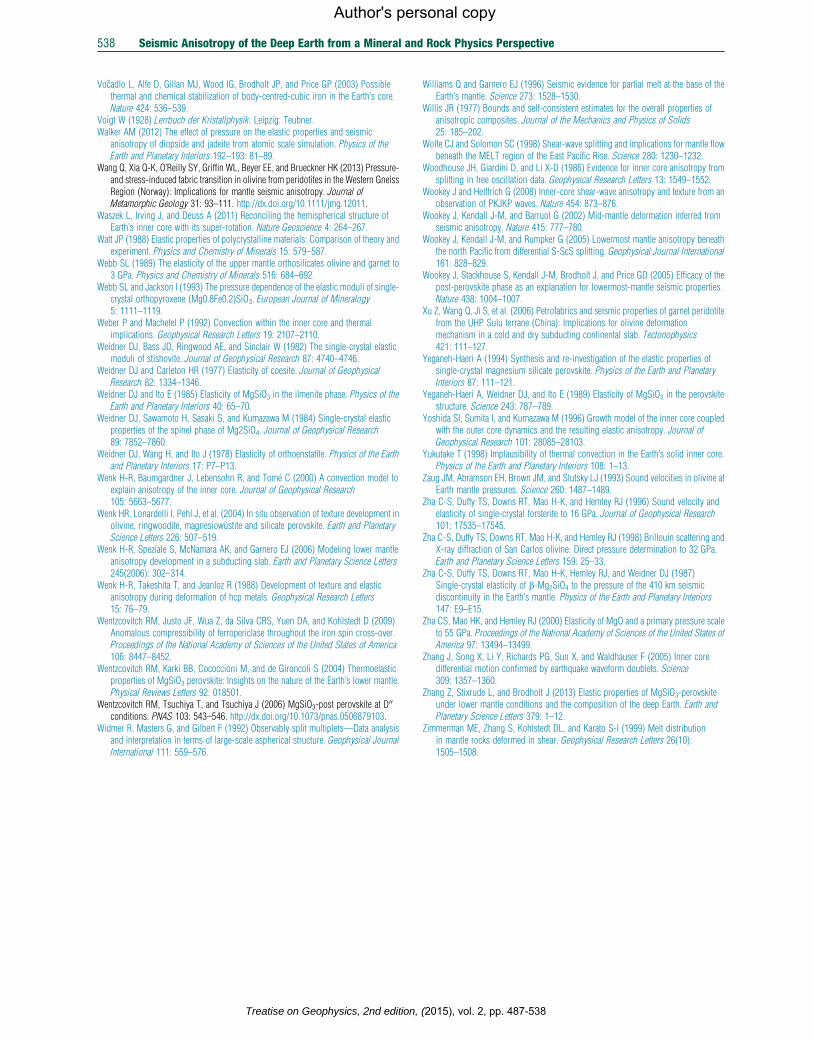
538 Seismic Anisotropy of the Deep Earth from a Mineral and Rock Physics Perspective
Author's personal copy
Vocadlo L, Alfe D, Gillan MJ, Wood IG, Brodholt JP, and Price GP (2003) Possiblethermal and chemical stabilization of body-centred-cubic iron in the Earth’s core.Nature 424: 536–539.
Voigt W (1928) Lerrbuch der Kristallphysik. Leipzig: Teubner.Walker AM (2012) The effect of pressure on the elastic properties and seismic
anisotropy of diopside and jadeite from atomic scale simulation. Physics of theEarth and Planetary Interiors 192–193: 81–89.
Wang Q, Xia Q-K, O’Reilly SY, Griffin WL, Beyer EE, and Brueckner HK (2013) Pressure-and stress-induced fabric transition in olivine from peridotites in the Western GneissRegion (Norway): Implications for mantle seismic anisotropy. Journal ofMetamorphic Geology 31: 93–111. http://dx.doi.org/10.1111/jmg.12011.
Waszek L, Irving J, and Deuss A (2011) Reconciling the hemispherical structure ofEarth’s inner core with its super-rotation. Nature Geoscience 4: 264–267.
Watt JP (1988) Elastic properties of polycrystalline materials: Comparison of theory andexperiment. Physics and Chemistry of Minerals 15: 579–587.
Webb SL (1989) The elasticity of the upper mantle orthosilicates olivine and garnet to3 GPa. Physics and Chemistry of Minerals 516: 684–692.
Webb SL and Jackson I (1993) The pressure dependence of the elastic moduli of single-crystal orthopyroxene (Mg0.8Fe0.2)SiO3. European Journal of Mineralogy5: 1111–1119.
Weber P and Machetel P (1992) Convection within the inner core and thermalimplications. Geophysical Research Letters 19: 2107–2110.
Weidner DJ, Bass JD, Ringwood AE, and Sinclair W (1982) The single-crystal elasticmoduli of stishovite. Journal of Geophysical Research 87: 4740–4746.
Weidner DJ and Carleton HR (1977) Elasticity of coesite. Journal of GeophysicalResearch 82: 1334–1346.
Weidner DJ and Ito E (1985) Elasticity of MgSiO3 in the ilmenite phase. Physics of theEarth and Planetary Interiors 40: 65–70.
Weidner DJ, Sawamoto H, Sasaki S, and Kumazawa M (1984) Single-crystal elasticproperties of the spinel phase of Mg2SiO4. Journal of Geophysical Research89: 7852–7860.
Weidner DJ, Wang H, and Ito J (1978) Elasticity of orthoenstatite. Physics of the Earthand Planetary Interiors 17: P7–P13.
Wenk H-R, Baumgardner J, Lebensohn R, and Tome C (2000) A convection model toexplain anisotropy of the inner core. Journal of Geophysical Research105: 5663–5677.
Wenk HR, Lonardelli I, Pehl J, et al. (2004) In situ observation of texture development inolivine, ringwoodite, magnesiowustite and silicate perovskite. Earth and PlanetaryScience Letters 226: 507–519.
Wenk H-R, Speziale S, McNamara AK, and Garnero EJ (2006) Modeling lower mantleanisotropy development in a subducting slab. Earth and Planetary Science Letters245(2006): 302–314.
Wenk H-R, Takeshita T, and Jeanloz R (1988) Development of texture and elasticanisotropy during deformation of hcp metals. Geophysical Research Letters15: 76–79.
Wentzcovitch RM, Justo JF, Wua Z, da Silva CRS, Yuen DA, and Kohlstedt D (2009)Anomalous compressibility of ferropericlase throughout the iron spin cross-over.Proceedings of the National Academy of Sciences of the United States of America106: 8447–8452.
Wentzcovitch RM, Karki BB, Cococcioni M, and de Gironcoli S (2004) Thermoelasticproperties of MgSiO3 perovskite: Insights on the nature of the Earth’s lower mantle.Physical Reviews Letters 92: 018501.
Wentzcovitch RM, Tsuchiya T, and Tsuchiya J (2006) MgSiO3-post perovskite at D00
conditions. PNAS 103: 543–546. http://dx.doi.org/10.1073/pnas.0506879103.Widmer R, Masters G, and Gilbert F (1992) Observably split multiplets—Data analysis
and interpretation in terms of large-scale aspherical structure. Geophysical JournalInternational 111: 559–576.
Treatise on Geophysics, 2nd edition,
Williams Q and Garnero EJ (1996) Seismic evidence for partial melt at the base of theEarth’s mantle. Science 273: 1528–1530.
Willis JR (1977) Bounds and self-consistent estimates for the overall properties ofanisotropic composites. Journal of the Mechanics and Physics of Solids25: 185–202.
Wolfe CJ and Solomon SC (1998) Shear-wave splitting and implications for mantle flowbeneath the MELT region of the East Pacific Rise. Science 280: 1230–1232.
Woodhouse JH, Giardini D, and Li X-D (1986) Evidence for inner core anisotropy fromsplitting in free oscillation data. Geophysical Research Letters 13: 1549–1552.
Wookey J and Helffrich G (2008) Inner-core shear-wave anisotropy and texture from anobservation of PKJKP waves. Nature 454: 873–876.
Wookey J, Kendall J-M, and Barruol G (2002) Mid-mantle deformation inferred fromseismic anisotropy. Nature 415: 777–780.
Wookey J, Kendall J-M, and Rumpker G (2005) Lowermost mantle anisotropy beneaththe north Pacific from differential S-ScS splitting. Geophysical Journal International161: 828–829.
Wookey J, Stackhouse S, Kendall J-M, Brodholt J, and Price GD (2005) Efficacy of thepost-perovskite phase as an explanation for lowermost-mantle seismic properties.Nature 438: 1004–1007.
Xu Z, Wang Q, Ji S, et al. (2006) Petrofabrics and seismic properties of garnet peridotitefrom the UHP Sulu terrane (China): Implications for olivine deformationmechanism in a cold and dry subducting continental slab. Tectonophysics421: 111–127.
Yeganeh-Haeri A (1994) Synthesis and re-investigation of the elastic properties ofsingle-crystal magnesium silicate perovskite. Physics of the Earth and PlanetaryInteriors 87: 111–121.
Yeganeh-Haeri A, Weidner DJ, and Ito E (1989) Elasticity of MgSiO3 in the perovskitestructure. Science 243: 787–789.
Yoshida SI, Sumita I, and Kumazawa M (1996) Growth model of the inner core coupledwith the outer core dynamics and the resulting elastic anisotropy. Journal ofGeophysical Research 101: 28085–28103.
Yukutake T (1998) Implausibility of thermal convection in the Earth’s solid inner core.Physics of the Earth and Planetary Interiors 108: 1–13.
Zaug JM, Abramson EH, Brown JM, and Slutsky LJ (1993) Sound velocities in olivine atEarth mantle pressures. Science 260: 1487–1489.
Zha C-S, Duffy TS, Downs RT, Mao H-K, and Hemley RJ (1996) Sound velocity andelasticity of single-crystal forsterite to 16 GPa. Journal of Geophysical Research101: 17535–17545.
Zha C-S, Duffy TS, Downs RT, Mao H-K, and Hemley RJ (1998) Brillouin scattering andX-ray diffraction of San Carlos olivine: Direct pressure determination to 32 GPa.Earth and Planetary Science Letters 159: 25–33.
Zha C-S, Duffy TS, Downs RT, Mao H-K, Hemley RJ, and Weidner DJ (1987)Single-crystal elasticity of b-Mg2SiO4 to the pressure of the 410 km seismicdiscontinuity in the Earth’s mantle. Physics of the Earth and Planetary Interiors147: E9–E15.
Zha CS, Mao HK, and Hemley RJ (2000) Elasticity of MgO and a primary pressure scaleto 55 GPa. Proceedings of the National Academy of Sciences of the United States ofAmerica 97: 13494–13499.
Zhang J, Song X, Li Y, Richards PG, Sun X, and Waldhauser F (2005) Inner coredifferential motion confirmed by earthquake waveform doublets. Science309: 1357–1360.
Zhang Z, Stixrude L, and Brodholt J (2013) Elastic properties of MgSiO3-perovskiteunder lower mantle conditions and the composition of the deep Earth. Earth andPlanetary Science Letters 379: 1–12.
Zimmerman ME, Zhang S, Kohlstedt DL, and Karato S-I (1999) Melt distributionin mantle rocks deformed in shear. Geophysical Research Letters 26(10):1505–1508.
(2015), vol. 2, pp. 487-538