SEISMIC ANALYSIS - Defense Technical Information · PDF filead-a261 001 february 1993 ug-0027 dtic electe sguide feb 2 2 199311 user's gud s seismic hazard analysis by j. m. ferritto

AD-A261 001

February 1993 UG-0027

DTICELECTE

SGUIDE FEB 2 2 199311USER'S GUD S

SEISMIC HAZARD ANALYSIS

by

J. M. Ferritto

NAVAL CIVIL ENGINEERING LABORATORYPort Hueneme, CA 93043-4328

Sponsored byOffice of Naval Technology

Approved for public release; distribution unlimited.

2 1 O

REPORT DOCUMENTATION PAGE Nf 070418

Pulbfc "ap tlng brden Ow fts cmslolebn 0o famw is ested to averge I h"ar per npome", incudlng mhe Oiw t@ revewieng ralucieln., sewm*V e&dtatng Otn 5m0 .geammng w meiiallfig te da neeed. end ln sai eIidg me €cain of Iihmnatian. Sn Wcamim ngedng ths brdon atkie er any otw aspect of tiscoaNcion inlaetMian, incklIng suggestin sor duckg m bthi a, to Washion Hedft"Ws Services. Dkfda'te fo lInmlcaon and PAW, 1215 Jefaon Davis i% wy,Suat 1204, AJlngton, VA 22202-4302, and to tme 0M of Managerned and Budget, Pawwaat Reduction PI (0704-0183). WashNgton. DC 20603.

1. ACENCYIS ONLY (LwvsL•bs) 2. IEPOKY TA1l EPNT TYPE DATES COVERED

I February 1993 Finak Oct 1992 through Feb 1993

4. MIX AN SUfIITLE 5. WhUNinG hMBER8

USER'S GUIDE - SEISMIC HAZARD ANALYSISPR - RM33F60-001-0106

t mUqMM WU - DN387338

J.M. Ferritto

7. PWONMOM1 ONOAMNZUM WM AM A0Of M L 5.PErFOMN OMAIUZAIOUREPORT NSUER

Naval Civil Engineering Laboratory560 Laboratory Drive UG-0027Port Hueneme, CA 93043-4328

0. SPONSOINGOWONITO AIENCY N*MEN AIM ADDORWW 106 3PMo8MNO AoUTMUNA0ENCY REPORT NUMBER

Office of Naval TechnologyArlington, VA 22217-5000

11. SUPPENW I NOTES

11w 0INSUrlOWNAVAILAUTY STATEMENT 12b. ODITBUllON CODE

Approved for public release; distribution unlimited.

1I. AS8TRACT PMwkmnur 200 wardj

An automated procedure has been developed to perform seismic analysis using available historic and geologicdata. The objective of the seismicity study is to determine the probability of occurrence of ground motion at the site.Response spectra and time history techniques are presented.

I & SLOOM MTIS Is. NLUnE OF PAE

Earthquake, seismic, response spectra, time history, site acceleration 1281t PiCE COOE

17. S0LM CLASRCATIOM I&. SecQfT C4ASSRICAIO 1. SECUF TLASIONAf 28 LJTAMIOU OF ABSTRACTOP PMOT OF TWO PAGE OF A2STRACT

Unclassified Unclassified Unclassified UL

NSN 7540-01-210416= Standard Form 2 (Rev. 240)Presaooed by ANS SO& 230-1S2105-102

INTRODUCTION - What is a Beismicity Btudy

The objective of a seismicity study is to quantify the leveland characteristics of the earthquake ground motion which pose arisk to a site of interest. The seismicity study will produce aprobability distribution of expected site acceleration for agiven exposure period and also give an indication of the frequen-cy content of that motion. The approach taken in this work is touse the historical epicenter data base in conjunction with geo-logic data where available to best estimate the earthquake recur-rence of a region or fault. This recurrence relationship is usedto determine the regional or fault contributions to the overallsite acceleration level. This becomes the basis for definitionof response spectra suitable for use in structural design andanalysis. The procedure utilizes three parts to accomplish thestudy. The first part creates a subset of earthquakes from thegeneral data base and plots all events within a specified region.The second part utilizes the epicenter data to perform a regionalanalysis determining the magnitude recurrence relationship forthe region which may be adjusted for geologic data where known.Additionally the program computes the probability of accelerationat the site location and gives plots of recurrence and accelera-tion data. The third part analyzes individual faults. It deter-mines fault magnitude recurrence and probability of accelerationat the site from an event on each fault specified. Geologic datamay be used to augment historical epicenter date. Each part willbe discussed in detail below.

GETTING STARTED

System Requirements

The Program is designed to run on standard desk top personalcomputers using the MS DOS operating system version 3 or higher.The following are required:

MS DOS version 3 or higher640 k system memory

Hard disk80287 math coprocessor

optional devices DTIC QRALI71 IlPMD

plotter irCQTLT ~r~~printer

The following plotters are supported: Ac-c~esoi Fot ....'

EPSON FX8O printer or compatible (used as plotter) NTIS CRA&I IHewlett Packard Laserjet printer or compatible DTIC TAbi

Hewlett Packard Plotters Unlno,,o:,cOtiHouston Instruments Plotters Justjf~c,

Tecktronix 4025ByDistribitlofl I

Avdidt'biity (C,.,les

Dil Avail -i'td, orOist Special1' ? .. . . ..

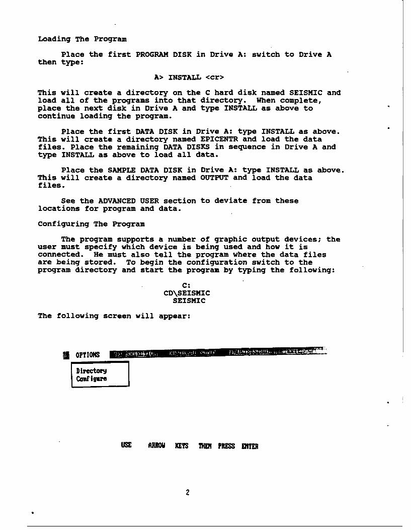
Loading The Program

Place the first PROGRAM DISK in Drive A: switch to Drive Athen type:

A> INSTALL <cr>

This will create a directory on the C hard disk named SEISMIC andload all of the programs into that directory. When complete,place the next disk in Drive A and type INSTALL as above tocontinue loading the program.

Place the first DATA DISK in Drive A: type INSTALL as above.This will create a directory named EPICENTR and load the datafiles. Place the remaining DATA DISKS in sequence in Drive A andtype INSTALL as above to load all data.

Place the SAMPLE DATA DISK in Drive A: type INSTALL as above.This will create a directory named OUTPUT and load the datafiles.

See the ADVANCED USER section to deviate from theselocations for program and data.

Configuring The Program

The program supports a number of graphic output devices; theuser must specify which device is being used and how it isconnected. He must also tell the program where the data filesare being stored. To begin the configuration switch to theprogram directory and start the program by typing the following:

C:CD\SEISMIC

SEISMIC

The following screen will appear:

O OPTION

USE AM EM M PRES ENTER

2

The program has five choices which form the opening menu:Options, Earthquake Selection, Regional Study, Fault Study, andExit. Use the LEFT and RIGHT ARROW keys which are on the numberpad keys with the 4 and 6 to move among the choices. Make surethe NUM LOCK key is off to permit the arrow keys to function.When the OPTIONS choice is selected a window opens giving twochoices: Directory, and CONFIGURE. Use the down arrow key tochoose the CONFIGURE choice then press ENTER (or RETURN). Thefollowing screen appears:

Enter Plotter DEV'ICE NUMIJBER 1

we User's anual e.g. LPT1 = I

Enter Plotter MODEL NUMBERsee User's Manual e.g. HP Lasejet =68

Enter Drive and Directory for EPICOTER files RMXESexample C:\EQUAKES

Enter Drive and Directory for OUTPUT files F:"I1IICexample C:\OUTPUT

Amj Changes? V /N

The DEVICE NUMBER refers to the port to which the hard copyplotting device is connected; see Table 1 for configurationoptions and check the manual for the hard copy plotting device.Enter the DEVICE NUMBER then press ENTER or DOWN ARROW.

The MODEL NUMBER can be obtained from Table 2a for thedevices supported by the program. Laser printers produce highquality plots rapidly and are recommended. Table 2b gives amatrix MODEL NUMBERs for various compatible printers which canbe used to obtain plots. Table 3 gives the recommendedconfiguration for specific devices. Enter the MODEL NUMBER thenpress ENTER or DOWN ARROW.

Type the directory name where the epicenter data files arelocated. If you used the INSTALL routine to accept the defaultdirectory creation then type:

C:\EPICENTR

Note the back-slash (\) key and the spelling of EPICENTR, 8letters without the E. If you chose to locate the programs elsewhere enter the following:

Drive letter:\Directory

example D:\EPIC

3

Table 1. Device Number

Device Output DeviceNumber Parallel Port

0 PMN: (PIN: is equivalent to LPTl:)31 LTl:2 LPT2:3 LFT3:

-onAsole-

99 CON: 1Comol 2

-serial ports-

device baud parity odclts "to1rprate bits bits

300 (XOM1: 300 N a 1

301 COlI: 300 0 7 1302 CCIO: 300 & 7 1

2200 CMWI: 1200 N 8 11201 COMI: 1200 0 7 11202 COwl: 1200 E 7 1

"800 CCNI: 4M0 N a"801 COMI: 4800 0 71480 CMHI: 4lM0 E 71

9600 COIl: 9600 N a 19601 COWl: 9600 0 7 19602 COHl: 9600 9 7 1

parity: NtEonoI-tve.

OmOdd

COW1:whdd 50 to value for COMl:

4

Table 2a. Model Number

Model Printer-Plotter-ScreenNumber Device Identification

0 Epson FX-80 Printer, single density.I Epson FX-S0 Printer, double dansity.2 Epson FX-80 Printer, double speed, dual

density.3 Epson FX-80 Printer, quad density4 Epson FX-80 Printer, CRT Graphics 1.5 Epson FX-80 Printer, plotter graphics.6 Epson FX-S0 Printer, CRT Graphics I.

10 Epson FX-1O0 Printer, single density.11 Epson FX-100 Printer, double density.12 Epson FX-100, double speed, dual density.13 Epson FI-100 Printer, quad d misty.14 Epson FX-100 Printer, CRT Graphics I.15 Epson FX-lO0 Printer, plotter graphics.16 Epson FX-100 Printer, CRT Graphics II.20 RP 7470A Graphics Plotter.30 HP 7475A Graphics Plotter.40 Epson 14-1500 Printer, single density.41 Epson TA-1500 Printer, double density.42 Epson 14-1500, double speed, dual density.43 Epson 14-1500 Printer, quad density.51 Houston Instrument DKP-51 MP or

DIP-52 MP Plotter, 0.001" step size.52 Houston Instrument DNP-51 MP or

DNP-52 HP Plotter, .005" step size.60 HP 2686 LaserJet Printer or LaserJet

PLUS printer, using A size paper(8.5" z 11") (216 mm x 280 mm).Drawing resolution: 75 dots per inch.

61 HP 266A LaserJet Printer, using 35 sizepaper (7.2" x 10.1") (182 = z 257 mn).Drawing resolution: 75 dots per inch.

62 RP 2686* LaserJet Printer, using A sizepaper (8.5" x 11") (216 me x 280 mn).Drawing resolution: 150 dots per inch.

63 HP 2686 LaserJet Printer, using 35 sizepaper (7.2" x 10.1") (162 ma x 257 mn).Drawing resolution: 150 dots per inch.

64 ip 2686" LaserJet Printer, using A sizepaper (8.5" x 11") (216 me x 280 mn).Drawing resolution: 300 dots per inch.

65 HP 2666A LaserJet Printer, using 35 sizepaper (7.2" x 10.1") (182 -e x 257 mn).Drauing resolution: 300 dots per inch.

continued

5

Table 28. (continued)

so UP 75605, VP 73853, or HP 75661 DraftingPlotter using ilse A/M6 to D/Al paper.Np 75350 Graphbcs Plotter using sizeA/M to 1/03 paper.SP 74OA ColorPro plotter using sizeUS/M paper.

65 SP 75835 or IP 73865 Drafting Plotterusing sise I/AO paper.

90 Tektronix 4025.99 JlN color graphics monitor (CRT).

Table 2b. Dot Matrix Printer Usage by Model

MlodelPr inter ------- -5a0 1 2 3 4 5 6 10 11' 12 13 14 15 16

EpeonlX-80 * * * * * 0 *apsom n-80 ••&pson *X-SO6*IN Printer * * * *Centronics am * * *Okidata 92 * * *RpsomU48 * * * * * *Epson 1-O00 . * • * * *Epson *l-O 0 0 * 0Okidata 93 0 0 * 0

* - The printer cam use this model number.

6

Table 3. Rec-oeded Configuration

Output device Device Model

Epson FX-80 0 5Epson UX-80 0 1IBM Printer 0 1Centronics GLP 0 1Okidsta 92 0 1Epson RX-80 0 1Epson FX-100 0 15Epson HX-100 0 11LQ-1500 0 41Okidata 93 0 11II DM5P1S 9600/9650 51HI DI1-52 9600/9650 51HP 744OA 9600/9650 80HP 7470A 9600/9650 20HP 747SA 9600/9650 30RP 7350A 9600/9650 80HP 73805 9600/9650 s0HP 75853 9600/9650 80/85HP 75865 9600/9650 80/85HP 2686A 9600/9650 60/61Tektronix 4025 4600/O850 90IBM color graphics .99 99

monitor

7

No spaces are allowed in the name. For further information seeyour DOS manual on sub-directory creation and naming. Press ENTERor DOWN ARROW to advance to the next item.

Type the directory name where the output files are located.If you INSTALLed the SAMPLE DATA you created a directory called:

C:\OUTPUT

If you did not then a directory has not been created. Select andtype a name for the output file location such as:

C:\OUTPUT

Remember this name; we will use it again. Press ENTER

Upon completion, you are asked if you wish to make changes.If everything is correct type N for no or else Y for yes andrepeat the data entry. Use DOWN ARROW keys to skip over accept-able answers and change only what is in error.

If you did not use the INSTALL for SAMPLE DATA do the following.When N for NO CHANGES is pressed the program returns to theOPTIONS WINDOW. Use the RIGHT ARROW key to EXIT. When out ofthe program create the OUTPUT LOCATION directory if one does notexist. Type the following:

CD\MD\OUTPUTCD\SEISMIC

SEISMIC

The opening screen will reappear as shown above. This time pressENTER to accept the DIRECTORY choice. A screen like the followingwill appear showing the earthquake epicenter files on disk.

DIRECTORY F:\EPIC\*.EIC

11 file(s) found

E2.EPC E9.EPCEI.EPC E9.EPCE3.EPC E18.EPCE4.EPC E11.EPCES.EPCE6.EPC17.EPC

Filename : E2.EPC

Use cuovr key to select file then press (EITER)8

Press ENTER to continue and a directory of the files in the

output location directory will appear:

DIRMTORY F:%SDATA-%.*

16 file(s) found

OIE.PL!T ItO.PL TEST.3P1TVO .PLT TUO.Ou .ESIPOSE.PLTTHREE.PLT TEST.30TONE.OUT TEST.AOTTVO.OU? IEST.IPTTHREE.OUT TEST.EQSEDO OHE.PL

Filename : ONE.PLT

Use mcur kegs to select file then press (ENTER)

Press ENTER to return to the OPTIONS window menu. We are nowready to begin a problem.

ZARTHQUAIAZ]• LCTION

The epicenter data base has been prepared from the NationalOceanic and Atmospheric Administration's data base. Each filecovers a specified region and contains date, latitude, longitudeand magnitude data. This section is used to create a subset ofearthquakes for a specific region from the main set of earthquakefiles. The program searches a rectangle specified by maximum andminimum latitudes and longitudes to find all events within thebox above the specified magnitude. To become familiar with theprogram, the user may advance to the EQ SELECTION. The follow-ing screen appears:

9

Spec lf.4 AreaRevise DataBegin A•nlusis

View ResultsPrint ResultsPlot ResultsSave Results

USE ARROW KEYS rM PRESS ENTER

Use the DOWN ARROW key and then choose REVISE DATA to see theexample problem. Press RETURN to accept each value unchanged.Then select VIEW RESULTS from the EQ SELECTION window to see theoutput file on screen. Selecting PRINT RESULTS or PLOT RESULTSwill print or plot the sample problem.

Specify Data

This choice permits data entry for a new problem. Selectingthis choice will overwrite previous data examples unleL3 theywere saved to a named file. You will overwrite the sample databut it can be copied from the original disk again if needed. Thefollowing screen will appear:

Enter flaximm Longitiude (Degrees) 121example 1M -8

Enter Minimum Longitude (Degrees) 113example 112.9

Enter Maximum Latitude (Degrees) 41example 46.0

Enter Hinimum Latitude (Degrees) 37example 34.9

Enter Site Longitude (Degrees) 115example 115.0

Enter Site Latitude (Degrees) 38,..example 38.6

Enter Ifininum Magnitude Cutoff 3.8example 3.8

Ang Changes? V / N

10

Enter the longitude and latitude for a rectangle bounding theproblem and the site longitude and latitude. The study area mustbe large enough to include distant events which can influence thesite. Geologic data should be consulted to look for boundariesof tectonic provinces. The site should be near the center of thestudy region unless otherwise required by a tectonic boundary.The region will form the boundary for selecting events to be usedin the study and are relevant to establishing the site seismicpotential. For regional studies consideration should be given toselecting an area large enough to establish the regional tectonicsetting. Enter the MINIMUM MAGNITUDE CUTOFF value, typically 3.0.Events below this level may not have been recorded and theirabsence distorts the relationship for recurrence.

The program computes the acceleration at the site locationfrom each epicenter location where a magnitude is specified inthe subset of earthquakes. This computation uses an accelerationdistance attenuation equation. The following attenuation rela-tionships for acceleration are included:

1. McGuire (1978)2. Trifunac and Brady (1975)3. Campbell (West) (1982)4. Campbell (East) (1982)5. Donovan and Bornstein (1978)6. Joyner and Boore (1981)

The user is has the option of selecting which to use. Since eachequation analyzes the data differently and since there is a largeuncertainty in ground motion results may differ depending uponthe equation selected. The user is encouraged to read the refer-ences. The following screen is used to enter the accelerationequation choice and the hypocenter depth if needed, usually 10miles.

I Hc cGire

2 Trifunac and Brady

3 Campbel (Western US)

4 Campbell (Eastern US)

5 Donovan and Bornstein

6 Jogner and Boorn

Enter depth to b•pocenter (miles) S

ENTER CHOICE FOR ACCELERATION EQUATION11

Once the acceleration equation data entries are completed, theuser is asked to select epicenter files to be searched . Fileshave been divided into regions to keep the search time to aminimum. A screen similar to the following is shown from whichthe user may move through the list using the ARROW KEYS,PAGEUP/DOWN KEYS and then press ENTER to select his choices.There is no limit to the number of choices.

Calif 114-119 31-32Calif 114-120 32-33Calif 114-121 33-34Calif

114-12 34-35

Calif 114-123 35-36Calif 114-123 36-37Calif" 114-123 37-39Calif 114-124 38-39Calif 114-125 395-46

Calif 114-125 48-41Calif 114-125 41-43

Press ESCAPE when done. The program then shows the choices andasks for confirmation.

YOU HAE SELECTED TH FOLLOU Iu RECOUDS:

7 Calif 114-123 37-388 Calif 114-124 38-399 Calif 114-125 39-4918 Ca if 114-125 49-4111 Calif 114-125 41-41

[S THIS CORRECT?. V,/I

12

Revise Data

If the user wishes to revise a number he may choose theREVISE DATA choice and will be given the same questions as in theSPECIFY DATA section with the previous choices. Press enter orDOWN ARROW to accept the value unchanged. Overwrite the revisedvalue completely to alter a number.

Begin Analysis

This choice begins the actual data search.

View Results

The VIEW RESULTS choice permits the user to see the outputfile from an analysis on the screen. It must be run after ananalysis has been performed and data exists.

Print Results

PRINT RESULTS prints the output files. The output consistsof a list of epicenters with the computed site acceleration forthat event, and a histogram of the distribution of acceleration.

THE FOLLOWING IS AN EXAMPLE OUTPUT

MAX LONGITUDE 73.000MIN LONGITUDE 69.000MAX LATITUDE 44.000MIN LATITUDE 41.000MIN MAGNITUDE .000MAX MAGNITUDE 9.000SITE LONGITUDE 72.000SITE LATITUDE 42.000ACCELERATION EQUATION .000

LIST OF SITE EPICENTERSYEAR LATITUDE LONGITUDE MB MS MO ML AVM DISTANCE ACCEL1976. 41.66 69.97 .00 .00 .00 3.00 3.00 106.776 .0031979. 43.98 69.80 3.80 .00 4.00 4.10 3.97 177.364 .0041977. 41.84 70.70 .00 .00 3.10 .00 3.10 67.614 .0061974. 41.70 71.50 .00 .00 .00 2.50 2.50 32.976 .0081976. 41.56 71.21 .00 .00 .00 3.50 3.50 50.660 .011

whereMB Body wave magnitudeMS Surface wave magnitudeMO Other magnitudeML Local magnitudeAVM Average magnitudeDISTANCE Distance event to siteACCEL Site acceleration computed estimate, g's

13

Plot File

This choice creates an epicenter plot for the region.Figure 1 is an example plot.

Save Results

This choice permits the user to write the input, output and plotfiles to a named file of the user's choice. This prevents thefiles from being overwritten.

14

73.00 69.00 W. 00 ,1.00

31 2

•3

Note: numbers are approximate magnitudes

Figure 1. Epicenter plot for region.

15

REGIONALL STUDY

Moving the RIGHT ARROW key to REGIONAL STUDY reveals thefollowing screen:

ERECIONAL STUDY

Specifr9 RegionRevise DataBegin Analysis

Uiew ResultsPrint ResulPlot ResultsSav ReultsResponse Plot

USE ARRON RES I=I PRESS M

This section is used to conduct a regional seismicity studytypically for eastern sites where faulting is not known It usesthe epicenter subset created previously . This section willestimate the level and characteristics of the earthquake groundmotion which pose a risk to the site of interest. We will usethe historical epicenter data base in conjunction with geologicdata where available to best estimate the probability of siteacceleration levels. This becomes the basis for definition ofresponse spectra suitable for use in structural design and analy-sis.

For a regional analysis the epicenter data base is used todefine the regional magnitude recurrence based on a log-linearfit of the data and the Richter A and B recurrence coefficientsare determined.

Log (N) = A + B M

The program allows the user to specify minimum cutoff magnitudeto enhance the fit. Generally the epicenter data base isdeficient on small events since events less than magnitude 3 maynot be large enough to be recorded at distant seimographstations. Thus a cutoff of 3 is usually used to insure the fitof the data is through the linear portion of the data. Figure 2illustrates the case in which the initial data did not use acutoff minimum magnitude. The line should be fit through thelinear portion. The program may be repeated, with the userspecifying the A and B coefficients based on his modification tothe computed fit of the data.

16

100.000 -- \ili

Ig10.000 -- -

Ij 1.00-

*too - - - -- -

. 010 _L

.001 --.0 1.0 2.0 3.0 4.0 5.0 6.0 7.0 8.0 9.0

HAGNITUDE

Figure 2a. Regional earthquake recuccence.

17

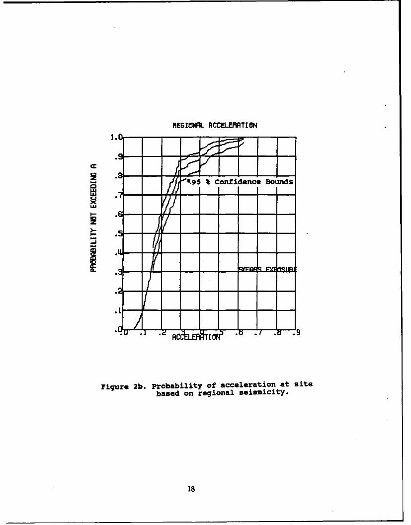
REGIONAL ACCELERFTION

1R5

E R•95 % Confidence Bounds

.5

.2

Figure 2b. Probability of acceleration at sitebased on regional seismicity.

18

Having established the magnitude recurrence relationship, a"floating" earthquake analysis is performed using a Monte Carlosimulation routine A series of events representing a 5000 yearexposure are randomly, spatially assigned with magnitude shapedby the recurrence relationship. A maximum cutoff magnitude maybe included to fit the tectonics of the region. A probabilitydistribution for a specified exposure period of acceleration atthe site location is computed. The simulation process is randomin location and includes the error associated with the earthquakeattenuation equations. A histogram of magnitude and accelerationis computed.

Use the DOWN ARROW key and then choose REVISE DATA to see theexample problem. Press RETURN to accept each value unchanged.Then select VIEW RESULTS from the window to see the output fileon screen. Selecting PRINT RESULTS or PLOT RESULTS will print orplot the sample problem.

Specify Region

From the REGIONAL STUDY window select SPECIFY REGION andpress ENTER. The following questions will appear:

Enter Mlaximum Longitiude (Degrees) 121examp le In2.a

Enter Mlinimum Longitude (Degrees) 116example 112.0

Enter Maximum Latitude (Degrees) 41examp [e 48.8

Enter Minimum Latitude (Degrees) 36example 34.0

Minimum Earthqpake Magnitude Cutoff 3example 3.8

Maximum Eartquake Magnitude Cutoff 8.5example 8.8

Enter Site Longitude (Degrees) 117example 115.0

Enter Site Latitude (Degrees) 38example 38.5

Any Chnges? Y / H

19

Enter the longitude and latitude of a rectangle to bound thestudy area. This may be a smaller than the region chosen for theEARTHQUAKE SELECTION discussed previously. Consider thetectonics of the region in selecting bounds for the study. Besure to include sufficient distance from the site so that allevents which can cause significant ground motion at the site areincluded. Enter the MINIMUM MAGNITUDE CUTOFF, usually 3 sinceevents less than 3.0 may not have been recorded and distortion ofthe recurrence estimation might result. Enter the MAXIMUMMAGNITUDE of the region.

As discussed above, enter the acceleration equation andhypocenter depth if needed, usually 10 miles. Enter the EXPOSUREPERIOD of the study in years.

I Mc Guire

2 Trifunac and Brady

3 Campbell (Western US)

4 Campbell (Eastern US)

5 Donovan and Bornstein

6 Joyner and Boore

IETER COICE FOR ACCELERATION niTION

Enter depth to hypocenter (miles) U

Enter Exposure Perion (Years) Uexample 58.9

20

At this point you will be asked whether to use theearthquake data base or to use regional recurrence, A and Bvalues. Enter Y to use the epicenter data. If N is enteredenter the values of A and B as shown here:

Do 9W wish to cnmp•te recurrence data

from the epicenter data base ()es or (H)o

If gou answer No, gou mst enter

Richter A and I values for the region

Your Choice? Y / H

Enter Richter A value 4.3exanple 4.2

Enter Richter B valueexmple -. 85

Revise Data

The user may revise data once entered by selecting REVISEDATA from the REGIONAL STUDY window. The same questions given inSPECIFY DATA are asked with the previous responses. Advancethrough the data using the DOWN ARROW. Overwrite the revisedvalue completely.

Begin Analysis


View Results


21

Print Results

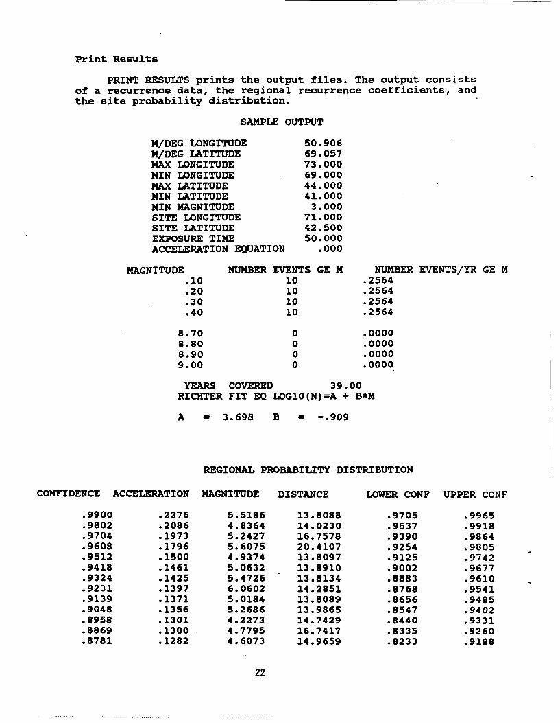
PRINT RESULTS prints the output files. The output consistsof a recurrence data, the regional recurrence coefficients, andthe site probability distribution.

SAMPLE OUTPUT

M/DEG LONGITUDE 50.906M/DEG LATITUDE 69.057MAX LONGITUDE 73.000MIN LONGITUDE 69.000MAX LATITUDE 44.000MIN LATITUDE 41.000MIN MAGNITUDE 3.000SITE LONGITUDE 71.000SITE LATITUDE 42.500EXPOSURE TIME 50.000ACCELERATION EQUATION .000

MAGNITUDE NUMBER EVENTS GE M NUMBER EVENTS/YR GE M.10 10 .2564.20 10 .2564.30 10 .2564.40 10 .2564

8.70 0 .00008.80 0 .00008.90 0 .00009.00 0 .0000

YEARS COVERED 39.00RICHTER FIT EQ LOGl0(N)-A + B*M

A = 3.698 B = -. 909

REGIONAL PROBABILITY DISTRIBUTION

CONFIDENCE ACCELERATION MAGNITUDE DISTANCE LOWER CONF UPPER CONF

.9900 .2276 5.5186 13.8088 .9705 .9965

.9802 .2086 4.8364 14.0230 .9537 .9918.9704 .1973 5.2427 16.7578 .9390 .9864.9608 .1796 5.6075 20.4107 .9254 .9805.9512 .1500 4.9374 13.8097 .9125 .9742.9418 .1461 5.0632 13.8910 .9002 .9677.9324 .1425 5.4726 13.8134 .8883 .9610.9231 .1397 6.0602 14.2851 .8768 .9541.9139 .1371 5.0184 13.8089 .8656 .9485.9048 .1356 5.2686 13.9865 .8547 .9402.8958 .1301 4.2273 14.7429 .8440 .9331.8869 .1300 4.7795 16.7417 .8335 .9260.8781 .1282 4.6073 14.9659 .8233 .9188

22

.8694 .1262 5.2475 15.1447 .8133 .9117

.8607 .1239 5.5734 15.8349 .8034 .9044

.8521 .1237 5.3539 18.6373 .7939 .8972more

HISTOGRAMS COVERING 5000.0 YEARS

NO. P(X) F(X) HISTOGRAM MAGNITUDE86 .086 .086 3.307 *

109 .109 .195 3.450 *********************************************73 .073 .268 3.593 *********************************************77 .077 .345 3.736 ************************************..........68 .068 .413 3.879 ***more

51 .051 .464 4.022 *********************************************66 .066 .530 4.165 *33 .033 .563 4.308 *34 .034 .597 4.451 **********************************36 .036 .633 4.594 ************************************35 .035 .668 4.737 ***********************************36 .036 .704 4.880 ************************************33 .033 .737 5.023 ******************31 .031 .768 5.166 *********20 .020 .788 5.309 ********************

moreNO. P(X) F(X) HISTOGRAM ACCELERATION

563 .563 .563 .007 *214 .214 .777 .021 ************************************ more

86 .086 .863 .036 *************47 .047 .910 .050 *********************************************18 .018 .928 .064 ******************13 .013 .941 .079 *************

9 .009 .950 .093 *********9 .009 .959 .107 *********6 .006 .965 .121 ******6 .006 .971 .136 ***4 .004 .975 .150 ****2 .002 .977 .164 **3 .003 .980 .179 ***2 .002 .982 .193 **2 .002 .984 .207 **1 .001 .985 .221 *0 .000 .985 .2362 .002 .987 .250 **

more

Plot File

This choice creates a plot of recurrence and siteacceleration probability for the region. Figure 2 is an exampleplot.

23

Save Results

This choice permits the user to write the input, output andplot files to a named file of the user's choice. This preventsthe files from being overwritten.

Response Plot

This choice creates a standard shaped site independentresponse plot on your plotting device, Figure 3. The user isrequested to provide the base ground motion level in g's.

24

DAMPING 2. 5, 7. AND 10 PERCENT1000.00

.1001 1 00

1010.00010

~ 10.00

.1.00

.01 .10 1.00 10.00 100.00

PERIOD (SEC)

Figure 3. Typical response spectra.

25

FAULTS STUDY

For western sites where fault locations are known in moredetail, a study can be performed by specifying the location of afault in terms of coordinates of several points defining linesegments. All earthquakes within a specified distance orboundary from the fault line under study are made a subset, andthe recurrence of the fault is calculated. A probabilityanalysis is then performed to calculate expected siteacceleration and causative earthquake magnitude and epicentraldistance for that fault. The program randomly selects theepicenter of an earthquake somewhere along the specified lengthof the fault. Using the fault recurrence data in terms ofRichter coefficients and maximum earthquake magnitude associatedwith the fault, the program determines and earthquake magnitudeand the length of fault break (assumed centered on theepicenter), and then calculates the distance of the site to thefault break (the epicentral distance and the hypocentraldistance). These distances, along with the acceleration-magnitude attenuation relationship with its uncertainty definedby the standard deviation for that level of motion, give the siteacceleration. The process is repeated using a Monte Carlo schemeto produce a list of site accelerations and related causativemagnitude and epicentral distance thus defining the site'sprobability distribution. It is important to note that theprogram is random for each and every fault in the following:

a) Location along fault length, 2 dimensionalb) Magnitude shaped by recurrence coefficientc) Acceleration level using mean and standard deviationrelationship of magnitude - distance

Provisions are included to use recurrence data from slipanalysis or regional seismicity in lieu of fault specific data.The program determines, tabulates, and plots the probability ofnot exceeding various levels of acceleration in the time periodspecified. These data are available for all individual faults, andthen are combined for all faults acting together. Thedetermination of total risk to the site is of importance forestablishing design levels.

A single recent large event may release strain built up overhundreds or thousands of years. As such, it might indicate aperiod of less activity in the immediate future. However, sincethe data base is relatively short, the return time for this eventmight be erroneously indicated as much less. For example, ifthis were a 500-year event and occurred during a 50-year database its return might be estimated at 0.02 rather than 0.002.The plotted data points and line of best fit are determined bythe computer analysis using regression analysis techniques.These should be reviewed and judgment used to adjust this type ofdatum point that will clearly plot significantly higher than thelinear portion of the recurrence data.

The procedure is intended to be repeated several times,

26

during which the engineer can compare geologic data and lines ofbest fit from historic data and converge on the best estimateusing his judgment.

The FAULTS STUDY window reveals the following choices:

bulse Data

Begin AnalEsis

view Results

Print ResultsPlot ResultsPlot faultsSaue DesultsRlesponse PlIot

Edit FaultsLst

USE ARBON MYS THE PRIMSENTER

Use the DOWN ARROW key and then choose REVISE DATA to see theexample problem. Press RETURN to accept each value unchanged.Then select VIEW RESULTS from the window to-see the-output fileon screen. Selecting PRINT RESULTS or PLOT RESULTS will print orplot the sample problem.

Specify Data

This is the data entry section for a new problem. Selectingthis choice shows the following screen:

27

Enter laximum Longitiude (egrees) lieexample 129.9

Enter Minimum Longitude (Degrees) 114examp Ie 112.9

Enter laximum Latitude (kereezs) ........example 49.9

Enter Minimum Latitude (Degrees)example 34.9

Minimum Magnitude Cutoff 3example 3.9

Enter Site Longitude (Degrees) .Texample 115.6

Enter Site Latitude (Degrees) 39example 39.9

Enter Exposure Period (Years) sail"exap le 5..9

Changes? V / N

Enter the longitude and latitude of a rectangle to bound thestudy area. This may be a smaller than the region chosen for theEARTHQUAKE SELECTION discussed previously. Consider thetectonics of the region in selecting bounds for the study. Besure to include sufficient distance from the site so that allevents which can cause significant ground motion at the site areincluded. Enter the MINIMUM MAGNITUDE CUTOFF, usually 3 sinceevents less than 3.0 may not have been recorded and distortion ofthe recurrence estimation might result. Enter the EXPOSUREPERIOD of the study in years.

28

Enter the acceleration equation to use as discussed above.

1 ftCesiz'

2 Trifwuc and Dzadi

3 Campbell (Vutemu US)

4 Canpbell (Eastern US)

S Dnovan and Uornatein

6 Joaer and Boore

I

ENTER CHOICE FOR ACCELERATION EQUATION

The user is then given a menu of known faults in the Californiaarea. This menu is NOT complete; but is meant as a vehicle toreduce data entry. The user may add to this list; this will bediscussed later.

SAM CLEMENTEPALOS VERDENEVPORT- INGLEVOODROSE CANYON

ELSINOREWITTIERSAN JACINTOCOYOTE CREEKSUPERSTITION PTSUPERSTITION HILLIMPERIALUAIINCI

SAN ANDREASXY LCCiISTIANITOSALISO

Use the ARROW KEYS or press the first letter of the fault namedesired to move throught the list. Press ENTER to select a fault;up to 15 faults may be selected.

29

The question is then asked whether to enter additional faults.If the answer is yes the following screen is shown:

Enter Fault Nam aem110example San Andreas

Enter Ilxinwu N1agnitude amexample 7.0

Enter Characteristic fanitudeexample 7.5

Enter Return Tim in Years.example 25•68

Enter Designator I or 2 or3 3I for 2 tine sevent2 for box segment3 for specification of Richter A and B

Enter Delth to Htpocenter (miles)example 5.8

Ang Changes? Y/N

Enter the name of the fault and the faults MAXIMUM MAGNITUDE.The CHARACTERISTIC MAGNITUDE is the magnitude which a geologicalevidence shows has a frequent history of occuring as a majorevent and the RETURN TIME requested is the return time of thatevent. This event is added to the seismicity computed by thehistorical data. The CHARACTERISTIC MAGNITUDE may exceed theMAXIMUM MAGNITUDE which is the cutoff for the recurrencecalculation based on the historical data or the inputcoefficients.

30

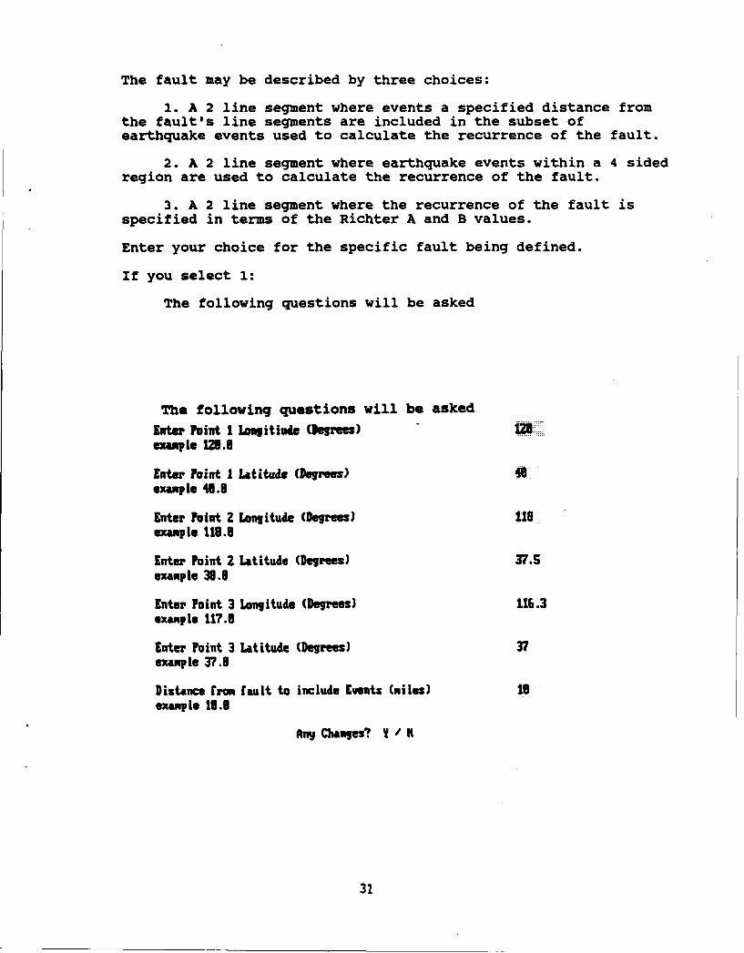
The fault may be described by three choices:

1. A 2 line segment where events a specified distance fromthe fault's line segments are included in the subset ofearthquake events used to calculate the recurrence of the fault.

2. A 2 line segment where earthquake events within a 4 sidedregion are used to calculate the recurrence of the fault.

3. A 2 line segment where the recurrence of the fault isspecified in terms of the Richter A and B values.

Enter your choice for the specific fault being defined.

If you select 1:

The following questions will be asked

The following questions will be asked

later Point I Longitiude (kirees) 123example 125.9

later Paint I Latitude (Degrees) 4example 48.8

Enter Point 2 Longitude (Degrees) 119example 118.3

Enter Point 2 Latitude (Degrees) 37.Sexamp te 39.5

Enter Point 3 Longitude (Degrees) I16.3exasp to 117.9

Enter Point 3 Latitude (Degrees) 37example 37.5

Distance from fault to include Events (miles) isexample 19.9

Am Changes? V / N

31

These define the line segments and distance away from the fault,

see Figure 4.

If you select 2:

The following questions will be asked as above.

SAW Point I Longitiue (Degrees) 123example 125.8

Enter Point I Latitude (Degrees) 48example 46.3

lnter Point 2 Lonvitude (Degrees) 119example 118.8

Enter Point 2 Latitude (Degrees) 3Sexample 39.8

Enter Point 3 Longitude (Degrees) 116!3example 117.8

Enter Point 3 Latitude (Degrees) .......example 37.3

Additionally coordinates for a 4 sided region must be entered.Start with the uppermost right point and proceed CLOCKWISE. SeeFigure 5.

ENTER 4 POINTS FOR BOX STARTING AT UIPPE RIGT IM GO CLOCVISEnter point I Lonitode (Degrees)example 128.9

Enter Point I Latitude (Degree,) 48example 46.8

Enter Point 2 Longitude (Degrees) 115.5example 118.0



Enter Point 3 Latitude (Degrees) 37.5examp le 37.8

Enter Point 4 Longitude (Degrees)example 129.5

Enter Point 4 Latitude (Degres ) 48

examp le 37.5

32

Figure 4. Two line segment model of fault with

distance from fault shown.

33

Figure 5. Two line sequent of fault with surrounding4-aided region.

34

If you select 3:

Enter the points for the 2 line segments as above.

Enter Point I Longitiude egree) 123examp le IZ.a

Enter Point I Latitude (Degrees) 48example 48.9

Enter Point 2 Longitude (Degrees) ,1texample 118.6

Enter Point 2 Latitude (Degrees) VXexample 38.5



Aug Changes? Y/fl

Then enter the A and B values.

Enter Richter A for Fault 449*example 4.8

Enter Richter B for Fault -.9example -. 89

35

Revise Data

The user may revise data once entered by selecting REVISEDATA from the FAULTS STUDY window. The same questions given inSPECIFY DATA are asked with the previous responses. The user mayrevise the data specified in the predefined faults list.

DO YOU UISH TO RE•ISE DATA FOR THE FAULTS

"U SELECTED FROM THE FIEDEFINED LIST

(Y)ES / (H)O

Selection of N for NO allows the user to accept or revisethe selection of faults from the predefined list of faults in themenu. The data for these faults can not be revised for thischoice. However, the user may revise the data for the faults heentered. Selection of Y for YES treats the predefined faults asif they were user entered and allows the user complete freedom tochange all values. In editing faults the user may skip a faultby pressing the ESCAPE KEY after the fault name appears ratherthan the ENTER or DOWN ARROW KEY. This advances to the nextfault leaving the previous fault's values unchanged.

NOTE AND WARNING

THE PREDEFINED FAULTS ARE REASONABLE FIRST ESTIMATES. THEYWILL NOT SUIT ALL CASE STUDIES. IN PARTICULAR, THE USER SHOULDPAY ATTENTION TO THE DEFINITION OF THE REGION SURROUNDING THEFAULT LINE TO INCLUDE EARTHQUAKE EPICENTERS FOR THE FAULTRECURRENCE RELATIONSHIP. THE INTENT IS TO INCLUDE ONLY THOSEEVENTS WHICH CAN BE ATTRIBUTED TO THAT FAULT AND EXCLUDE THOSEFROM OTHER FAULTS. BASED ON YOUR SPECIFIC PROBLEM IT MAY BENECESSARY TO CHANGE THE SELECTION MODE FROM A STANDARD DISTANCEAWAY FROM THE FAULT TO A QUADRILATERAL DEFINITION. AFTER APRELIMINARY ANALYSIS FIRST RUN SOLUTION, THE USER SHOULD EXAMINEEACH RECURRENCE CURVE AND INCORPORATE GEOLOGIC DATA. THE SLOPE OFTHE RECURRENCE LINE SHOULD BE CHECKED TO INSURE IT PASSES THROUGHTHE LINEAR PART OF THE EVENTS DATA. THE USER SHOULD REVISE THEFAULT DATA FOR THE ALPHA AND BETA COEFFICIENTS COMPUTED FROM THEINITIAL PRELIMINARY ANALYSIS. THIS ITERATION CONTROLS THEQUALITY OF THE ANALYSIS. THE ACCURACY OF THE ANALYSIS IS AFUNCTION OF THE EFFORT SPENT BY THE USER TO DEVELOP THE MODEL.THE PROGRAM HAS THE CAPABILITY OF PRODUCING HIGHLY ACCURATERESULTS.

36

Begin Analysis


View Result3


Print Results

PRINT RESULTS prints the output files. The output consistsof fault recurrence data, the fault recurrence coefficients,and the fault and total site probability distribution.

SAMPLE OUTPUT

M/DEG LONGITUDE 57.710M/DEG LATITUDE 69.057MAX LONGITUDE 119.000MIN LONGITUDE 115.000MAX LATITUDE 34.500MIN LATITUDE 32.000MIN MAGNITUDE 3.000SITE LONGITUDE 117.360SITE LATITUDE 33.300EXPOSURE TIME 50.000ACCELERATION EQUATION .000SAN CLEMENTE

INDIVIDUAL FAULT STUDY

FAULT COORDINATES

118.700 32.200118.300 32.800117.800 32.650

FAULT MAX CREDIBLE EARTHQUAKE 7.70

FAULT EPICENTERSLONGITUDE LATITUDE MAGNITUDE DIST ACC

117.800 32.583 4.500 55.645 .018117.833 32.800 4.000 44.015 .017117.833 32.716 4.400 48.699 .020117.866 32.800 3.100 45.221 .009

more

AVE ACCELERATION .0110MAX ACCELERATION .0378

37

EARTHQUAKE RECURRENCE

MAGNITUDE NUMBER EVENTS GE M NUMBER EVENTS/YR GE M.10 45 .6164.20 45 .6164.30 45 .6164.40 45 .6164

8.70 0 .00008.80 0 .00008.90 0 .00009.00 0 .0000

YEARS COVERED 73.00

RICHTER EQUATION LOG10(N) = A +B M

A = 1.640 B= -. 601

FAULT REGION ACCELERATION PROBABILITY

CONFIDENCE ACCELERATION MAGNITUDE DISTANCE LOWE R CONF UPPER CONF

.9900 .3014 7.2624 30.0969 .9705 .9965

.9802 .2364 6.7600 30.0901 .9537 .9918

.9704 .2084 6.0210 34.3689 .9390 .9864

.9608 .1984 7.3362 30.2334 .9254 .9805

.9512 .1799 6.7060 30.1197 .9125 .9742

.9418 .1795 5.9095 30.5953 .9002 .9677

.9324 .1606 6.6048 53.9805 .8883 .9610

.9231 .1571 7.4193 55.4437 .8768 .9541

.9139 .1548 6.9925 31.2901 .8656 .9485

.9048 .1306 6.7041 34.9663 .8547 .9402

.8958 .1292 7.5633 30.1013 .8440 .9331

.8869 .1287 5.6727 30.0893 .8335 .9260

A SIMILAR DATA TABULATION IS GIVENFOR THE TOTAL PROBABILITY ACCELERATION

FROM ALL OF THE FAULTS

Plot File

This choice creates a plot of recurrence andprobability data for each fault and the total site probability ofacceleration. Figure 6 is an example plot.

38

100.000 --- - -

10.000

LIl

j1.000 - - - - -L

.100

1 0.0101

Original line

2.0 3.• 0 1.0 2.0 3.0 q.0 5.0 6.0 7.0 8.0 9.0

MP•NITLEE

Note: The user should review the fit of the recurrence datashown by the line. This line should pass through the linearportion of the data. Sometimes when the number of events islimited or the minimum event is not specified the line maymiss that region. The user should then rerun the problemrevising the fault data by entering the A and B values froma new fit correctly through the data.

Figure 6a. Recurrence for a fault.

39

FFRULT I

.71

Figure 6b. Site acceleration probability from one fault.

40

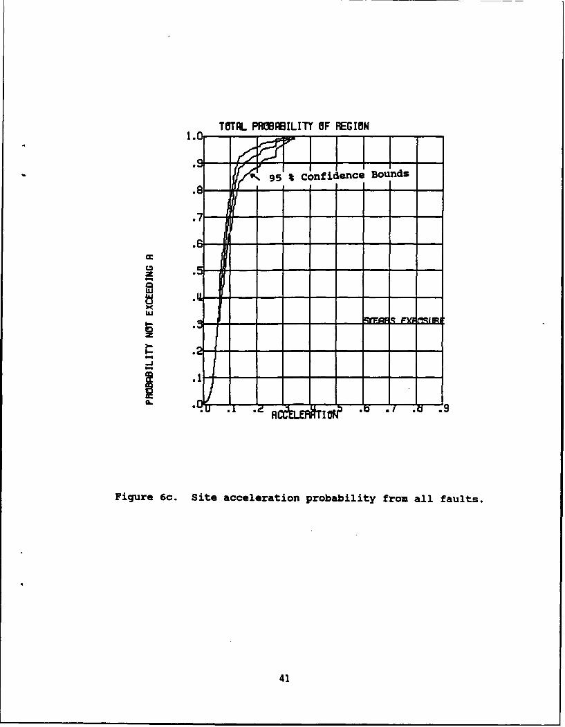
TOTAL PR1BRBILITY OF REGION1.0 2 ---

95 % Confidence Bounds

.7--

wtjUi

Il

Figure 6c. Site acceleration probability from all faults.

41

Plot Faults

This choice creates a plot of the faults entered in theSPECIFY DATA or REVISE DATA option. The epicenters in theEQUAKES file are plotted also. This choice requires that thedata be specified for the faults and the epicenter file becreated. However the analysis need not be performed, so this maybe used to check the events near faults.

The plotting procedure draws the grid of the regionspecified and then draws the faults and plots the epicenters.Often the fault extends beyond the region specified. IT IS NORMALIN SUCH CASES TO SEE AN ERROR MESSAGE STATING UNPLOTTED VECTORSOR CLIPPED VECTORS for the elements which go beyond the plotboundaries.

Save Results

This choice permits the user to write the input, output andplot files to a named file of the user's choice. This preventsthe files from being overwritten.

Response Plot

This choice creates a standard shaped site independentresponse plot on your plotting device, Figure 3. The user isrequested to provide the base ground motion level in g's.

Edit Faults.Lst

This option permits the user to change the values of thedata used to define the faults in the predefined faults listwhich appears as a menu from which the user may select faults foran analysis. Appendix A explains how to use this option and alsoexplains how to calculate the recurrence coefficients, A and Bfrom a recurrence plot. The appendix gives a list of faults andthe recurrence plots for all the faults defined in the FAULTS.LSTdata file of predefined faults. The user may add to this list.

NOTE recurrence plots for faults with predefined recurrencecoefficients are not plotted to save time; refer to Appendix Afor the plots.

42

Discussion of Faults

Seismometers have been installed near known active faults torecord microearthquakes. The events recorded range in magnitudefrom 0.5 to 1.5 and closely trace the faults. There are alsoregions where few microearthquakes occurred. The San Andreasfault north of the Sargent fault exhibits less activity thansouthern portions, perhaps indicating it is locked. However,sufficient microearthquakes have occurred to show thecontinuation of the fault. It may be reasoned that a smallfailure might occur before a major rupture occurs;alternatively,a large number of microearthquakes demonstrate active creep thatmay be sufficient to prevent sizable strain accumulation andpreclude a large event.

Since earthquakes are associated with faults, it might bethought that epicenters should precisely overlay the faultlocation. This is not the case, because the distribution ofseismometers is uneven and has changed with time. There arelimitations in the accuracy of the techniques used to locateepicenters, principally from variations in assumed propagationvelocities. Further explanation for the location of epicentersbeing off their associated fault comes from the simplified modelused to locate them. The center of earthquake energy is locatedat the focus. For an inclined fault, the surface location(epicenter) is a distance removed from the surface faultlocation. It is only in vertical faults that one might expectthe epicenter to lie on the fault.

Krinitzsky (1974) concludes that earthquakes can be relatedto existing faults and that the.possibility of formation of newfaults should not be considered in design. Large earthquakesrequire fault breaks of considerable distance. The uncertaintiesassociated with earthquakes generated from faults not previouslyknown can occur only for small events. Generally in the westernUnited States, the extent of geologic investigation precludes alarge fault from remaining unknown. However, there areuncertainties associated with eastern earthquakes. For example,causative faults responsible for the New Madrid earthquakes of1811 and 1812 have not yet been identified. This may be theresult of insufficient geologic investigations. The importanceof considering the extent and quality of geologic investigationsis evident.

A period of demonstrated quiescence over a geological timeperiod indicates inactivity of the fault and probable continuedinactivity. However, inactivity over a period of historicrecording (50 to 100 years) does not imply future inactivity.Rather it may point to a "locked" region through which a majorfault rupture may propagate. Two earthquakes to produce damagein southern California (Arvin-Tehachapi 1952; San Fernando, 1971)occurred on faults lacking major historic activity. With theexception of the San Jacinto fault system every known eventgreater than magnitude 6 in southern California has occurred on afault without prior major historic activity. It must be

43

recognized that the accuracy of an incomplete data base is verylimited when extrapolated for return period greatly exceeding thelength of the period of recorded data. Furthermore, aftershocksmust be distinguished from main shocks. An area having recentlyundergone a large event, which releases strain built up forhundreds or thousands of years, is probably safe against thatsize release in the near future. Thus a recent event on a faultmight actually indicate safety in the immediate future ratherthan an indication of activity. A single event by itself cannotgive an accurate measure of return time. The limitations of thehistoric data base can be reduced by considering the geologicdata available to assist in the definition of fault activity.

Faults are classified into several types according- to therelative displacement of the sides of the fault. Three principaltypes are normal, reverse, and strike-slip. The main fault mayappear as a single break or as a parallel series of breaks.Surface rupture may or may not occur. Variations in displacementoccur along the fault. Some fault displacement occurscontinuously at a very slow rate and is termed as "creep". Creeprates have been established for some active faults in California.Estimates of earthquake recurrence can be sometimes made byobservation of fault displacements of exposed layers. in a trench.From age dating it is possible to identify the age of variousstrata and also to identify layer displacements.

ASSESSMENT OF GROUND MOTION ATTENUATION RELATIONSHIPS

A study was performed evaluating the significance anddifference of available earthquake attenuation relationships.Data, although apparently plentiful, are actually very limited.Events are recorded by strong mot-ion accelerographs often locatedwithin structures. The effect of the response of the structureoften influences the reading. The assessment of the location andseparation distance of many early recorded events is ofquestionable accuracy. Many researchers create subsets of thedata often defining their own meanings to distance and magnitudeand often limit the inclusion of records to specific conditionssuch as rock sites or events of only a limited magnitude range.Campbell (1982) for example computes in his relationship theaverage acceleration of the two horizontal directions. Campbellstates that the maximum direction value should be 1.13 times thecomputed value. Joyner and Boore (1981) use the seismic momentas the basis for magnitude determination while Campbell useslocal magnitude for events less than 6.0 and surface wavemagnitude for events greater than 6.0. Each investigator usesjudgment and perception of the elements incorporated into theformulation. This subjective approach makes seismic attenuationprediction more of an art since the scatter in the data is large.Recent work suggests that magnitude may not have the samesignificance for ground motion levels close to a fault as it doesat greater distances. The analytical procedures generally assumemotion to be related to magnitude and distance as independentvariables. However, it is recognized that they are notindependent. At close distances to the causative fault,

44

magnitude is not a controlling factor for ground motion in eventsof sufficient size with fault breakage over tens of kilometers inlength. Local effects dominate at these close distances. It isat greater distances that magnitude assumes the usual significantrole. However, the researcher must exercise care in treatment ofthis phenomena since an untendable position might occur that datacould be extrapolated to show magnitude 7.0 events at closedistances might produce lower ground motions than magnitude 6.0events at the same distance.

It is significant that each of the researchers citedconsiders the uncertainty in the data and allows for computationof the standard deviation of the acceleration. This must beincorporated in risk analysis procedure and has been done in thecomputer programs.

A topic of discussion is the significance of peaks inaccelerograms. It may be argued that these have little effect onthe responses of a structure and that some measure of aneffective acceleration should be used. Some suggest use of 0.65times the peak represents an effective level. Others choose amore complex approach taking levels of motion which compose 90%levels of motion based on histogram distribution of all peaks ina record. Although such approaches are indeed based on fact thatstructures do not respond significantly to single peaks, theytend to ignore the usual engineering approach which utilizes aground motion level to define a spectra. The spectra performsthe function of giving an effective level of motion in thefrequency response region of the structure. It is thus suggestedthat reduction of ground motion levels for use in creation of aspectra should not be done but rather the spectra willautomatically perform this task. The risk analysis procedure inthe program makes use of mean response data and the uncertaintiessuch as occur in nature. To reduce the reported levels would beunconservative. It is substantially better to utilize a seriesof spectra from earthquake records to "average" effectiveacceleration levels rather than arbitrarily "throw away" aportion of the record. This is particularly significant sincethe engineering pract5ice for scaling spectral values is in termsof peak values and until some other value is fabricated andagreed upon it will remain the only value clearly established todefine the record. The engineer tasked with design applicationsmust exercise caution in listening to the academics postulatingimproved techniques and not offering a corresponding basis forutilization of the existing spectral data base. Without a database converted to some measured effective acceleration level theengineer would not be able to scale spectra and would be severelylimited in characterization of a site.

Data reported by Chung (1978) was used in a study to comparecomputed and measured accelerations with distance. Records onbuildings and vertical records were excluded. As can be seen,there is significant scatter. The standard deviation is:

45

Mean StandardEquation Deviation* Deviation

McGuire -. 005 .089Trifunac and Brady +.008 .105Campbell (West) -. 059 .111Campbell (East) -. 041 .101Donovan and Bornstein -. 042 .104Joyner and Boore -. 056 .111

* Minus - underestimates data.

The McGuire equation appears to have the best fit and leastbias of the data. The analysis of the variances shows that thereis a 90% confidence that the McGuire relationship shows asignificant difference from the rest, that is that within theaccuracy of the data the differences in equations is meaningful.However, strictly speaking, this comparison is not exact becausedifferences exist in the definition of distances and magnitudes.Chang uses epicentral distance. This is not significant at largedistances. In an attempt to determine the significance andsensitivity to definitions of distance and magnitude, the Joyner-Boore data base of 183 records was used for comparison (based onclosest distance).

The data set used by Joyner and Boore was also studied. Themean and standard deviation of the equations are:

Mean StandardEquation Deviation* Deviation

McGuire +.001 .0901Trifunac and Brady +.076 .1885Campbell (West) -. 027 .0936Campbell (East) -. 013 .0913Donovan and Bornstein -. 014 .0844Joyner and Boore -. 021 .0830

* Minus - underestimates data.

The McGuire equation has the least bias. The standarddeviations except for the Trifunac and Brady equations arestatistically about the same. It is not surprising that theJoyner and Boore equation fits this data best since it wasformulated from the data.

The significance of selection of the earthquake attenuationequation is primarily in the determination of separationdistances. McGuire and Donovan for example define therelationship in hypocentral distance, Trifunac and Brady in terms

46

of the epicentral distance and Campbell and Joyner and Boore interms of the closest distance to the fault. For risk analysis offaults where the site tends to be located near one end of thefault the selection of a relationship based on the shortestdistance will tend to give higher values. Caution should be usedin selecting equations like Joyner and Boore or Campbell thatutilize the shortest distance for use in regional studiesinvolving floating earthquake epicenters (and not least distanceto site). These relationships will report significantly loweraccelerations that are not correct. To illustrate thesignificance of the attenuation relationship a study was made ofa site 0.5-miles from the Hayward fault. Results for the 225-year return time are:

Joyner and Boore .535g

Campbell .540g

McGuire .396g

Donovan and Bornstein .382g

The first two use shortest distance; the last 2 usehypocentral distance. The hypocentral distance is thought to bea better representation. This example presents extremeconditions not usually encountered.

A study of the Monterey area was made. Six faults wereconsidered; results are given as follows for the 225-year returntime site acceleration composite risk from 6 faults:

McGuire 0.2802g

Joyner and Boore 0.3404g

Campbell 0.2832g

For comparison Thenhaus, et al. computes for the same site

100-year return time 0.20g

500-year return time 0.50 to 0.62g

The following projections can be made. The 100-year returntime acceleration, 0.2g, has a 61% probability of not beingexceeded in 50 years. This translates into a ratio of 0.70 ofthe 250-year return time acceleration. The projected 250-yearacceleration would be .02/.07 or 0.286g. The 500 year returntime acceleration, 0.5 - 0.62g, has a 90% probability of notbeing exceeded in 50 years. This translates into a ratio of 2.0of the 250-year return time acceleration. The projected 250-yearacceleration would be 0.5/2.0 to 0.62/2.0 or 0.25 - 0.31g. Theseresults agree favorably with those computed by the program(McGuire) and suggest a value of about 0.28g. It can be seenthat the Joyner and Boore value of 0.34, based on closest

47

distance of fault to site, produces more conservative results.

To summarize, all the above cited equations have beenimplemented into the program in a correct consistent manner aseach author intended taking account of each authors definitions.

48

PROGRAM LIMITATIONS

The EARTHQUAKE SELECTION routine can process 20,000epicenters to the file EQUAKES.

The REGIONAL STUDY can input 20,000 epicenters.

The FAULTS STUDY can input 20,000 epicenters and 30 faults.Each fault can have up to 5,000 epicenters associated with it.

To keep the computational process manageable within thelimits of a desktop computer tradeoffs had to be made in MonteCarlo process. As can be seen the 95 percent confidence boundsincrease as the probability of not exceeding the accelerationincrease. This program is intended to-give an estimation ofearthquake motions up to the 90 percent probability of not beingexceeded in 50 years with high confidence. This program is notintended to be used to predict 5,000 year or 10,000 year events.

The user constructs a model of the seismicity of a region towhich epiceters are assigned, recurrence relationships computedand ground motion probabilities determined. It should be obviousthat if the user failsto include sufficient fault definition themodel will lack those details and their contribution to thesite's expected motion. Regional studies can not be substitutedfor fault studies with the same level of accuracy. While this isa simple but accurate analytical tool in the hands of a trainedengineer it can be misused by the uninformed.

WARNING

CHECK YOUR RESULTS TO INSURE LESS THAN 20,000 EVENTS WERE SELECT-ED.The program will display the number of events selected and thenumber of events read. If 5000 events were read reduce yourarea if possible or break the analysis into 2 parts. Failure todo this will result in the omission of all events beyond the 5000event limit thus reducing the coverage.

FOR TER ADVANCED USER

Data and Output Files

The following shows the input data files created and theoutput results files for each section of the program.

INPUT OUTPUT

CONFIGURATION DEVICE.CFG

EARTHQUAKE SELECTION ONE.IN ONE.OUTEPICENTR.LST ONE.PLT

epicenters .EPC EQUAKES

49

REGIONAL STUDY TWO.IN TWO.OUTEQUAKES TWO. PLT

FAULTS STUDY THREE.IN THREE.OUTFAULTS.LST THREE.PLT

Files with the extension .EPC are epicenter files. Fileswith the extension .IN are data iiles created by the program.Files with the extension .LST are files supplied to the userwhich the user can modify; these will be discussed later. Fileswith the extension .OUT are output files to be printed. Fileswith the extension .PLT are plot files.

When files are saved the above files are copied to disk witha new name specified by the user as follows:

EARTHQUAKE SELECTIONONE.IN XXXXXXXX.1INONE. OUT XXXXXXXX. IOUONE . PLT XXXXXXXX. lPT

REGIONAL STUDYTWO. IN XXXXXXXX. 21NTWO. OUT XXXXXXXX. 20UTWO. PLT XXXXXXXX. 2PT

FAULTS STUDYTHREE.IN XXXXXXXX.31NTHREE.OUT XXXXXXXX.30UTHREE.PLT XXXXXXXX. 3PT

The program is set to use the standard names in the left column.To restore a saved data, output or plot file for use copy thefile to the standard name as follows:

COPY XXXXXXXX.1IN C:\SEISMIC\ONE.IN

COPY XXXXXXXX.IPT ONE.PLT

Note that the INPUT files are stored in the PROGRAM DIRECTORYand the OUTPUT and PLOT files are stored in the DATA/RESULTSDIRECTORY. The program will re-run or revise the last caseexecuted with the standard names. To revise or re-run a case,only the INPUT file (.IN) need be copied to the standard name.

Epicenter Files

The epicenter data base is broken down into separate filescovering small regions to minimize search time. The user may addto the list of epicenter file by editing the file EPICENTR.LSTwhich contains the number of files and for each epicenter filein the data base the file description and file name.

Number of Epicenter FilesDescription , xxxxxxx.EPC

50

The epicenter data files contain data in the followingformat:

Year Col 5 to Col 8 F4.0Latitude Col 20 to Col 24 P5.3Longitude Col 26 to Col 31 F6.3BM Body Magnitude Col 36 to Col 38 F1.2SM Surface Magnitude Col 54 to Col 55 F1.1OM Other Magnitude Col 61 to Col 63 F1.2LM Local Magnitude Col 83 to Col 85 F1.2

Note no decimal points used.

51

REFERENCES

Campbell, K.W. (1982). "A preliminary methodology for the re-gional zonation of peak ground acceleration," in Proceedings ofthe Third International Earthquake Microzonation Conference, June1982. Seattle, WA., University of Washington, 1982.

Chung, F. K. (1978). MPS73-1 State of the art for assessingearthquake hazards in the United States catalogue of strongmotion eartquake records, Wtaerways Experiment Station, Vicks-burg, MS, April 1978

Donovan, N.C. and Bornstein, A.E. (1978). "Uncertainties inseismic risk procedures," Journal of the Geotechnical EngineeringDivision, American Society of Civil Engineers, no. 103, pp 869-887.

Gutenberg, B and Richter, C.F. (1954)/ Seismicity of the earthand associated phenomena, 2nd edition. Princeton, NJ, PrincetonUniversity Press, 1954.

Joyner, W. B. and Boore, D. M. (1981). Peak horizontalacceleration and velocity from strong-motion records includingrecords from the 1979 Imperial Valley, CA, earthquake, BulletinSeismological Society of America, no. 71, pp 2017-2038.

Krinitzsky, E. (1974). Fault assessment in earthquakeengineering, Army Engineering Waterways Experiment Station,Miscellaneous Paper S-731. Vicksburg, MS', May 1974.

McGuire, R. K. (1978). "Seismic ground motion parameterrelations," in Proceedings of American Society of Civil EngineersJournal Geotechnical Engineering Division, no. 104, pp 481-490.

Richter, C. F. (1958). Elementary seismology. San Francisco,CA, W. H. Freeman Co., 1958, pp 768.

Trifunac, M. D. and Brady, A. G. (1975)/ " On the correlation ofpeak acceleration of strong motion with earthquake magnitude,epicentral distance and site conditions." in Proceedings of theU. S. National Conference on Earthquake Engineering, Ann Arbor,MI, University of Michigan, 1975.

52

Seismic Hazard Analysis

Appendix

Fault Data Base

A-1

THE FAULTS.LST FILE

The FAULTS.LST file contains a list of over 60 faults inCalifornia whose location and recurrence have been defined. Thislist is meant as a starting point and is by no means complete.The values used are based on seismicity studies conducted ofvarious regions of California. The values are best estimatesbased on the data available at the time they were made. Programusers are encouraged to review the data and change the valuesbased on more current data. To edit the data select the EDITFAULTS.LST option from the FAULTS STUDY menu.

The user may advance through the list by pressing the ESCAPEKEY; once the-fault to be revised is found, press ENTER and movethrough the data using the ARROW KEYS; enter the revised numbersand proceed through the list. The program writes the old versionof the list to a file labeled FAULTS.BAK as a precaution.

The remainder of this appendix gives a procedure tocalculate the Richer recurrence coefficients, A and B from therecurrence plots. Note the program will attempt to fit therecurrence data calculated from the fault events as best aspossible. The recurrence line should pass through the linearportion of the data and usually have a B value, slope of theline, on the order of -. 90, the minvs indicating downwarddirection. Use this as a guide in evaluating the computerresults. The computer generated recurrence line is controlled bythe minimum magnitude allowed in the analysis and the distanceparameter which controls which and how many events to include inthe calculation of recurrence for that fault. When geologic datais available, plot the data on the recurrence plot. Then movethe line upward at the proper slope to include the geologic datapoints to increase fault recurrence if the geologic data soindicates.

The program gives the user a great deal of flexibility inproducing a valid analysis. Care must be exercised to developthe correct seismic model of the earthquake activity of a region.

Format of FAULTS.LST

The format for the file is as follows

Number of Faults

For each fault Line 1Fault Name

For each fault Line 2Maximum Magnitude, Characteristic Magnitude, Return timeHypocenter depth (miles)FAULT TYPE (1 ,2 or 3)Longitude Point 1

A-2

Latitude Point 1Longitude Point 2Latitude Point 2Longitude Point 3Latitude Point 3Distance From Fault (miles) for Type 1 or A value

for Type 30 for type 1 or B value for Type 3Characteristic MagnitudeReturn Time for Characteristic Magnitude

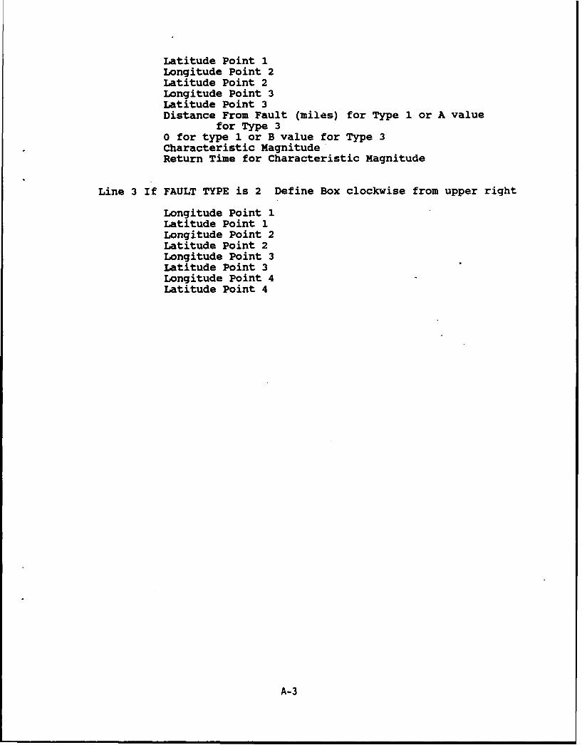
Line 3 If FAULT TYPE is 2 Define Box clockwise from upper right

Longitude Point 1Latitude Point 1Longitude Point 2Latitude Point 2Longitude Point 3Latitude Point 3Longitude Point 4Latitude Point 4

A-3

Computation of A'and B values is illustrated by the following:

log10 (N) a A + B*M

A z lolO (intercept at Mn0) H = 0 N = 112

A = lOglo (112) = 294921

B = slope of line (must be negative)

B _ 00 (112) - 10310 (.001) 2.04921 - (-3)7.77 - 0

7.=7

B = 0.65

B = -0.65 negative decreasing

B = A+3

Maguitude at .001 intercept

Value a 1U. A A - LoglO(1lll.6)

!0000J --

go .300O•SM0. 0000

- -

0~(n

Q-

Z 0 1. 000- - -- - -

tUi

7.77

3.00, F0 0 60 7. . ..0 1.0 2. MCNI iUODES' . 2

A-4

00 0

00

H0

9-4 00 0

Z44 alE- 0 0.

04 0 0 0

OH 00P-

E4 E-u r rI z hih r il Z E- 'j

EAra ZW1 O ~Z U ~ z3~CJH OM W HM-

undHo. 4mwEDW64wHN~lwCO CA' CmO

~Z Ee Z H rzZi Z sU%,Ui

a 41 0Hse

H

0a to0 zc

z in4 0 06 - 3 0

u W 1 00O 0 uUWRWZý -30w2W Z-4jNj044WUOOO0

H. ".A N4 z>x to z 09~wMr~~4

WMHI ýImm = W OX~pZ i mu m ZZ

0 - Nmv 0 % 0 0 f-Nr~mm vow r

A-5ZC

124 119

3 7

, I\"t

Fgr -1 Fut inrgo 12 19, 32-3

,ý A

I "- -

I- .1 I.-_-

Fiue32 Fut inrgo 2 1,3 -37

____ __ __ _ _-_A-6

119 \ \I _ _ _ _ _ _ _ _ _ _ _ _ 11 4

""" \31 30-

1 -S3234

ix

"50 - 23

A-7-.-J - "• - --7

0 ý7

3 A-7

124 119

41 31

II3i

I I

Figure A-3. Faults in region 124 -119, 37 -42.

77

6 I

3Kb 2

A-B

j19 114

- I

1

Ficure A-4. Faults in region 119 - 114, 37 - 42.

S543

\A-

\ A-9

100.000

Of

aX

041 10.000

a

I• 1.00

S .010

0

Fault - BANNING Maximum Maanitude 7

Fault Lonqitude /Latitude CoordinatesPT1 117.21 ,34 PT2 116.79 ,33.92 PT3 116.39 ,33.83

Figure A-S . Faullt recurre~nce.

A-10

100.000

00 10.000 --

a - - -

04

14

1 ".000

.00

0 6. 7.0 8.- 9.0

Magquitudo

Fault - BIG PIKE Maximum Maqnitude 7.6

Fault Longitude / Latitude CoordinatesPTI 119.85 °34.67 PT2 119.36 ,34.68 PT3 119 ,34.8

V i gU re A- 4 . ]Fault re curre nce.

A-11

100.000

0 10.000i"

04

0

10.000

Is .I'4

0 .101

410

.0 1.0 2.0 3.0 -. 0 5.0 6.0 7.0 8.0 9.0

Masgnitude

Fault - BLUE CUT Maximum Magnitude 7

Fault Longitude / Latitude CoordinatesPTI 116.25 ,33.9 PT2 115.79 ,33.91 PT3 115.38 ,33.93

]Pigl~e A--7 • aU3lt rec¢rrEence.

A-12

V 100.000

0- 10.000-

r4

,a

1 .00 _

R

0

1 010S.00

0 1.0 2.0 3.0 -.0 0 7.0 -.0 9.0

Magt

Fault - CAMPROCK Maximum magnitude 7

Fault Longitude /Latitude CoordinatesPTI 116.82 ,34.77 PT2 116.7 , 34.68 PT3 116.55 ,34.55

Figure A-S . Fault recurrenceo

A-13

100.000"4j

.94

010.000

0

1.000 - -i- -

P

• m

.01

64.00

Fiur - - - - -Val - -urene

A51

S100.000., \

0

S10.000 - •

a1 1.000 -

E4

4 .I00

S .100 -

Mantud

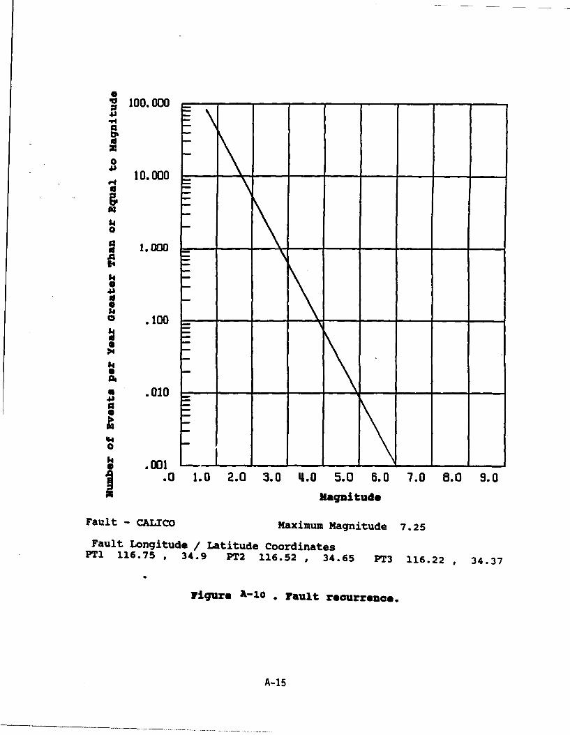
Fault - CALICO Maximum Magnitude 7.25


Figure A-10 . -au-t reaurrence.

A-15

93 100. 000

xz

10.0 -0

14

0

.00

01084

0

.1001 - -

0 . 1.0 2,.0 3.0 4.0 . 0 ,6.0 "7.0 8.0 9.0

Fault - COYOTE CREEK maximum Magnitude 7

Fault Longitude / Latitude CoordinatesPTI 116.52 ,33.46 PT2 116.27 ,33 .26 PT3 115.99 ,33.02

Figure A-11 . PaUlt recurrence.

A-16

o 100.000

*64140

I I.

.0100---

q.

0

S1.0 2.0 3.0 -5.0

. agnitude

Fault - DEATH VALLEY Maximum Magnitude 7

Fault Longitude / Latitude CoordinatesPTI 117 ,36.53 PT2 116.84 ,36, PT3 116.3 ,35.6

rigueO A-12 - IraUlt reCKrrEeco@.

A-17

E4 . .. .

100.000

•.e .

bi

041 10.000

0

S-O1.000- - - M n -.

A-1

34

.01

.00

-a0 1 1. -. -. . . . . . .

A11

S100.000

*64

0'

10.000 -

S.010

0

-1000 1.0 2.0 3.0 -.0 - -0a 6.0 7.0 8.0 -.-

Fault - EIMERON Maximum Magnitude 7.2

Fault Longitude / Latitude CoordinatesPT1 116.54 ,34.55 PT2 116.4 ,34.44 PT3 116.26 ,34.28

FigueO A-14 . Fault reaurrence.

A-19

,u 100.000"4,

0

10.000W

0

I. wOO,,

14

54

.41

Fault FURNACE CREEK Maximum Magnitude 8.25

Fault Longitude / Latitude Coordinates_PTI. 118.1 ,37.64 PT2 116.85 ,36.51 PT3 116-73 ,35.98

]PiqUrO A-I5 . PaUlt reoureonco.

A-20

"45

0

5 - --

a 1.00I ---

.010=

'4

.1 0--.0 1.0 2.0 3.0 4.0 5.0 6.0 7.0 -. 0 9.0

Magnitude

Fault - GARLOCK Maximum Magnitude 7.75


PigllZO A-16. Fault EOIEIIo

A-21

100.000

04

41.0

I .010

0

ii ~mag/nitude

Fault - GREEN VALLEY aCONCORD Maximum Magnitude 7


]PiglrS A-27 . Flault reaurreEnceo

A-22

,i oo. ooo- ----

100.I000

0

4 10.000-

0

1.000 - - - - - - - -A

646

S .100 --- - -

.01

U .0010----

-0 1.0 2.0 3.0 L.0 5.0 6.0d 7.0 8.0 9.0

Fault - HARPER Maximum Magnitude 7

Fault Longitude / Latitude CoordinatesPTl 117.59 ,35.31 PT2 117.23 ,35.1 PT3 116.92 ,34.9

Figure A-is.* Fault recurrence.

A-23

100.00043

"4,

0. 10.000I--

0

1.000 - - - - -7 - -

A4-a .100 --

34

0.

000

I .0 1.0 2.0 3.0 11.0 5.0 8.0 7.0 8.0 9.0Magnitude

Fault - HAYWARD Maximum Magnitude 7.5

Fault Longitude / Latitude CoordinatesPT1 122.37 ,38 PT2 122.15 ,37.73 PT3 121.74 ,37.27

Figure A-19 * Fault recurrence.

A-24

S100.000

04)10.000 --

1I

• 1.000 -

'4

.01

0

.00 - - -

Fault - HEALDSBURG Maximum Magnitude 6.75

Fault Longitude / Latitude CoordinatesPT1 122.89 ,38.67 PT2 122.64 , 38.37 PT3 122.45 ,38.17 |

N(

Figure A-20 - Fault recurrence.

A-25

"' •• .0 0 - --

100.00041

.010.

A

0

.10.000 - -- n -. 5

.01

6-

.41

0 .1 0 1 . 0 -. -. -. a. . . . .

6-2

'~100.000-

0

H 10.000 --

0

1.000 - - -

.14

.010

0 -

.00

0 1.0 2.0 3.0 4.0 5.0 6.0 7.0 6.0 9.0

Maqnitude

Fault - HOSGRI Maximum Magnitude 7Fault Longitude / Latitude Coordinates

PTI 121.5 , 35.9 PT2 121.1 , 35.5 PT3 120.75 , 34.9

FigUGe A-22 - Fault reaurrence.

A-27

S100.0004j".4 U\0

V 10.000

F4

540

a 1.000 - -5 -.- - - .0

A-2

•464

41

.10010 . . .0 40 50 60 . . .

A-2

'~100.000-

4A

0.0 10.000

-I "40

1 . Io0E4

04

a .010

0

.00

.O 1.0 2.0 3.0 .0 50 .0 7.0 8.0 9.0Magnitud- -

Fault - INYO MOUNTAIN Maximum Magnitude 7.5

Fault Longitude / Latitude CoordinatesPT1 117.95 ,36.92 PT2 117.81 , 36.66 PT3 117.11 ,36.2

Figure A-24- Fault reourrenceo

A-29

'~100.000 --

14j

"4

Id041 10.000 - ---

--

.100

SN..20001

.0 1.0 2.0 3.0 4.0 5.0 6.0 7.0 8.0 9.0

Kagnitude

Fault - LENWOOD MaxiimumMaqnitude 7.25

Fault Lonqitude / Latitude CoordinatesPT1 117.1 ,34.88 PT2 116.85 , 34.65 PT3 116.5 ,34.3

~Ie

F~iq~r A-23. FPault reourrgnoe.

A-30

SI00. 00,

0

a o.ooo - - ,

04'

10.000.-

54u

0

a 1.000 - -- - - - -. -

54 -

64A6

PA-3

.00

.0101 -- --

I 0 1.0 2.0 3.0 tl.0 5.0 6.0 7.0 6.10 9.0Magnitude

Fault - LIKELY FAULT Maximum Magnitude 7.5

Fault Longitude / Latitude CoordinatesPTI 121 ,41.56 PT2 120.64 ,41.25 PT3 120.27 ,40.9

1figUZO A-26 F ault reoUrrence.

A-31

100.000 .

r4

0

1.000

I/

S.100

64

0

1.001 -

- 11.0 2.01 3.01 4.0 .O. 7.0 8.0 9.01Raqnitude

Fault - LOCKAR Maximum Magnitude 7.5

Fault. Longitude /Latitude CoordinatesPT1 117.76 ,35.21 PT2 117.39 , 35-02 PT3 117.1 .34.AQ

Figure A-27. Fault recurrence,

A-32

'4• •

1 100.000

ty

0

M4 10.0m0

I.o o54

0

1.0100

- " 1. . . 40 50 60 7.0 . .

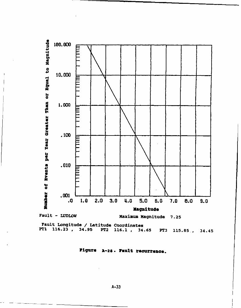
Fault - LUDLOW Maximum Magnitude 7.25

Fault Longitude / Latitude CoordinatesPTI 116.23 ,34.95 PT2 116.1 e34.65 PT3 115.85., 34.45

IPig•r A-28 • Vault: reaureEnce.

A-33

S100.00043".4a __0

1 .10.000

'-4

540

S1.000 - -

d

64

- u.100 -- - - - -

8-3

a .010 - - - - -- - -

0

I .0 1.0 2.0 3.0 I.0 5.0 6.0 7.0 8.0 9.0Magnitude

Fault - MALIBU RAYMOND maximum Magnitude 7.5

Fault Longitude / Latitude Coordinates

PT1 118.94 ,34.04 PT2 118.45 *34.04 PT3 117.45 *34.18

Figure A-29. * ault reourrenco..

A-34

100.000.,J"*4

0

10.000:-

14a1.000 - - - -- - -

$4

.01

o .1001 -F

U 00 -. 2.0 -. - -0 - -.0 70 B.3 S

Fault - mENDOCINO "Maximum Magnitude 7.5


Figure A-30. F&ult reaurrenco.

A-35

6 m

100.000

r4

1 .0100,,

*14

a

IIt

94

04

.01

Fault -MONO LAKE &HILTON Maximum Magnitude 6.75

Fault Longitude /Latitude CoordinatesPTI 119.2 ,38.16 PT2 119 , 37.73 PT3 118.56 ,37.25

719=6~ A-31 - Pault reaurrgeei0.

A-36

V 100.000

1 -X0

10.000"14

i -

$40

S1.00-

34

64

.01

0

04 1® 1\ 1 1. K I.00

A-3

U 0 0 -. -. -. -. 5.0 6.- -080 .

I~~Fgr .A1. -2032.0 Faul0 5.0 .0 70 8. .

A- 37

'~100.000--

43

010.000

.4

0

1.001 --- ~

l 0 1.0 2.0 3.0 4.0 5.0 6.0 7.0 B. 0 9.0KagnJituda

Fault - OAKRIDGE Maximum Magnitude 7.5

Fault Longitude /Latitude CoordinatesPTI. 119.•24 ,34.•23 PT2 119.•05 ,34.35 PT3 118.85 ,34.38

FiqUr* A-33* F~ault realreonceo

A-38

'• 100.0004.'

0'

• 10.000

040

1.000.0- - - -. . -. . -.

3-3

I4 I.

.010

.100 - - --

* 0 0 1- - - --. .0 50 60 7. . .

4.'iud

IT 10210 2. 3.03 T 1 1.1. 3 .0.00 7. 10 .04 36.07

Frigure A-34 - Fa&ult reaUrrenae.

A- 39

f 100.000

0

4 •10.000

0

1.000 - - -- - -

94

84

.I._

0I.00

0 1.0 2.0 3.0 -.0 5.0 6.0 7.0 -.0 9.0

Kagnitude

Fault - OWENS VALLEy Maximum Magnitude 8.25

Fault Longitude / Latitude CoordinatesPT1 118 ,36.23 PT2 118.25 , 37.06 PT3 118-36 ,37.6

FIr:UEdi J-35 - Fault reaurrEence.

A4

A-4

100.000 - - - - - - - - -

th

0Soo10.000

1.00E-4 1.00 - -- - - -

. I00

a .010

54

040

. 1

a

i 0 1.0 2.0 :3.0 4.0 5.0 6.0 7.0 8.0 9.0

M/agnitude

Fault - OZENA Maximum Magnitude 7.5


Figure A-36 • Fault reculrrence.

A-41

100.000 -

b%

0

S10.000

0

1.000 0 20 •0 0 50 . .

A

.4j

64

14

64

.001

*i r A030 -Fal- -urec.

A-4

100.000 - . -. -

0%

0j o10.000

U-'i

0

0

.1 0 00 -- - - - -

.1454j

0.01

Fault - -AAMN -ON - a u -antd -.2

Fault Longitude / Latitude CoordinatesPTI 117.4 ,36.33 PT2 117.3 ,36 PT3 116.96 ,35.6

PigUre A-34. •'r&ult reaurrenae.

A-43

Sm m m m • m m mm m m m n m m m

61 00.000

*6.

0

4 10.000

I .010

0

1.000 1-

-0 .0o . . . . 6.0 7.0 8.o 9.0Mantud

Fault - PIKE MOUNTAIN Maximum Magnitude 6.75


Figure A-39 . Fau3lt rOCUrrERoO.

A-44

100.000

043 10.000r4

$40

1.000 --

E4

S .0100di0

.1001 - -- -

0 1.0 2.0 3.0 .0 50 .0 70 80 9.0

Magnitude

Fault - PINTO MOUYNTAIN Maximum Magnitude 7.-5

Fault Longitude / Latitude CoordinatesPTI 116.6 ,34.03 PT2 116.35 , 34.13 PT3 115.88 ,34.1

FigureO A-40. Vault recurenOceO.

A-45

S100.000

04j 10.000

.4

I.541

010

U .0100 - - -- -

a

000

f Magnitude

Fault - PISGA1 Maximum Magnitude 7.25

Fault Longitude /Latitude CoordinatesPTI 116.49 ,34.85 PT2 116.23 , 34.47 PT3 115.9 ,34.1

FigEEo A-41 . Vault racsurrezice.

A-46

a

S100.000

.9_

0

10.10 20 3.0.0.0 60 700. .

Fault - PLEITO Maximum Magnitude 7


]J'g~leI A-42 . IF&Ult realrrenae.

A-47

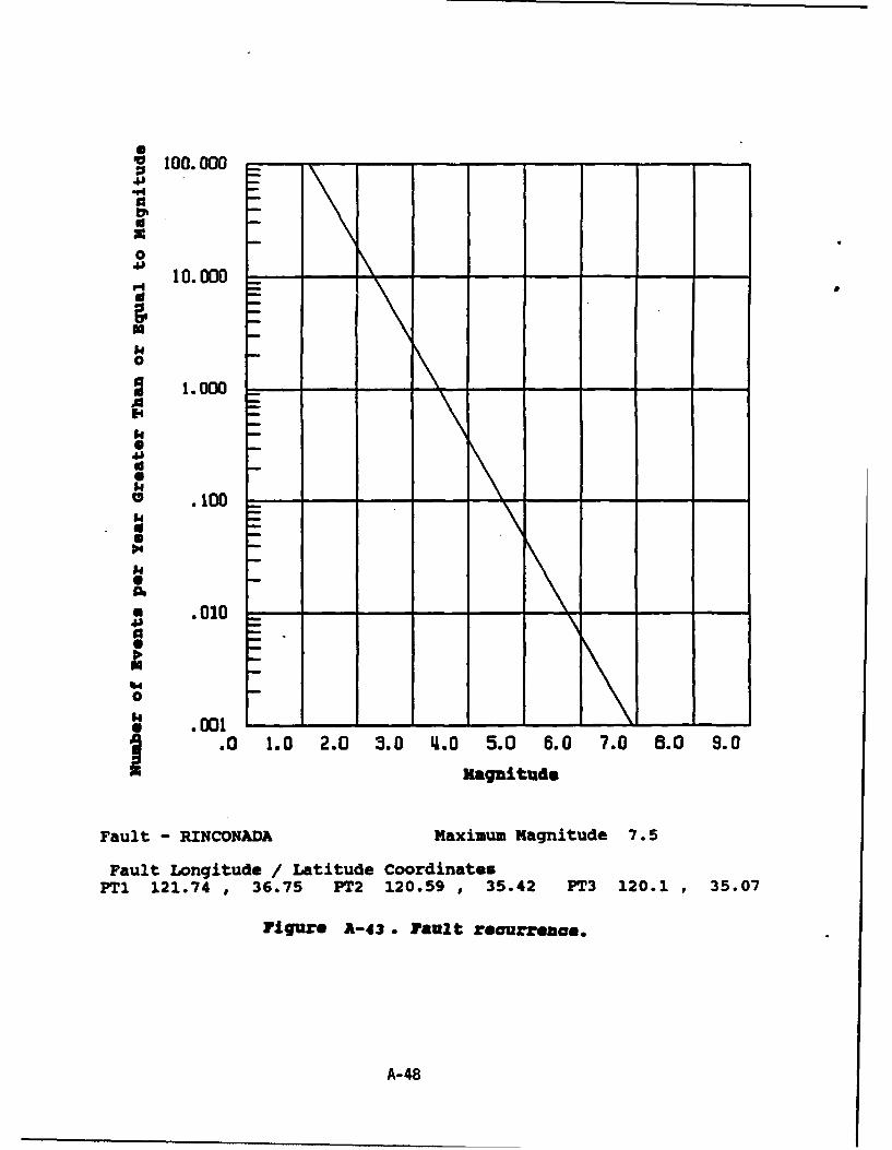
f 100.000

DO

M

0

10.000 -

S- \

S . I00

.010

0

Fault - RINCONADA Maximum Magnitude 7.5


Figure JL-43.- Pault roaurrenao.

A-48

100.000

41 1 .0

*14

0 .1000

.00

0 10 2.0 - 3.0 8.0 9.0

mtagnil.tudo

Fault - ROSE CANYON Maximum Magnitude 7.1

Fault Longitude / Latitude CoordinatesPTI 117.35 ,33 .06 PT2 117.28 , 32.87 PT3 117.05 ,32.54

Figurle A&-44.- Fault recurrence.

A-49

S100.000

Sz

4i

041 10.000P4

540

S.o1. 00

.01

164

I. e

0

410

Tiur A-45 -a eurne

A05

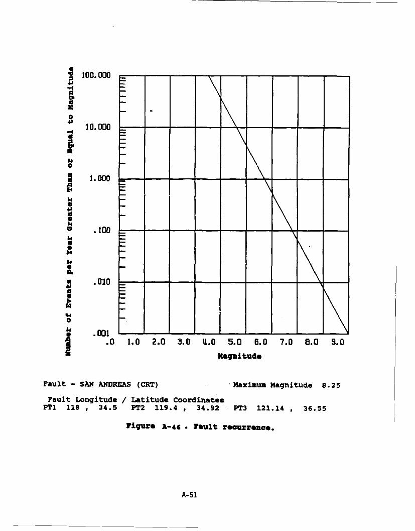
'~100.000 - - -- - - - -

010.000

E-4

II

0

1.001 -

.0 10 20 30 40 5. . . . .

A-5

S100.000

0 10

43

0

3 10.000

A40

1 .001

- . . .0 40 50 60 . . .

A-5

100.000

0V 10.000

0

S 1.000 - -

.01

5-5

a 1.0 - . -. . . .0 70 E. .

A-5

1I00.000

S o10.ooo

1.1000.• -

41

*14

.O0 1.0 2.0 3.0 4.0 5.0 6. 7.0 8.0 9.0aagi

Fault - SAN CAYETANO + MaxXmum Magnitude 6.75


rigjure A-49 • Fault recureEnce,

A-54

100.000

4J 10.000

0\S1.000 _

.r4

.00 -

I-I

1.00 ----

-. l.0 1.0 2.0 3.0 " 4•.0 5.0 6.0 7.0 8.0 9.0

Magnitude

Fault - SAN CLEMENTE Maximum Magnitude 7.7


IFigure A-SO • Fault reculrrence.

A-55

100.000

.dJ

0

01 1.000

0 .010

Q0

.000 - -. 0 5.0 6.0 7.0 8.0 9.0

Mlagnitude

Fault - SAN GABRIEL Maximum Magnitude .7.7


Figulre A-S1 o Fault recurrence,

A-56

S100.000

timx

0u 10.000""A4

a

14

.01

.14

0 1 0 1.0 -. -. -. 5. -. . . .

A-5

..0 .... -.-.--.

1 100.000 --

41

X

0

"43 10. 000

0

A

S.0101 .001

.O 1.0 2.0 -3.0 .0 5.0 7.0 8.0 -. 0

Magnitude

Fault - SAN JACINTO Maximum magnitude 7.5'

Fault Longitude / Latitude CoordinatesPT1 117-62 ,34.32 PT2 116.9 , 33.75 PT3 116.13 ,33.26

Figure A-53 . Fault recureEnce.

A-58

100.000 - -- -- - -

44

1000

1.00840

84

14

.00

Fal - SAN -UA -a' u -agniu-e-

A55

S100.000

01 0. 000 - - - - - - - - -

1

N

P .1 -

.000 --- -4101

U

0 1.0 2.0 -3.0 .0 5.0 6.0 .0 8.0 9.0

lKagnituds

Fault - SANTA CRUZ ISLAND Maximum Magnitude 7


Figure A-ss, Fault r'eaurtrenoe.

A-60

' 100.000

ON

0

10.000-

64

64

0

0 .000 1.0 2.0 3.0 4.0 5.0 6.0 7.0 8.0 9.0

magni~tude

Fault -- SANTA SUSANAI' Maxinum Magnitude 6.5

Fault Longitude / Latitude CoordinatesPT1 118.74 34.35 PT2 118.28 , 34.26 PT3 118.03 ,34.15

IrigUrO A-56 • Fault reanlrrence.

A-61

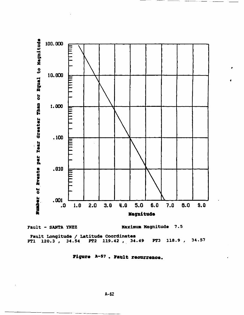
100.000

4j 10.00041.0

0

10.00-

• o .100 ,

. 010

001

.0 1.0 2.0 3.0 O4.0 Og 5.0 .0" 7.0 8.0 9.0

Fault - SANTA YNEZ maximum Magnitude 7.5

Fault Lonqitude / Latitude CoordinatesPT1 120.3 ,34.54 PT2 119.42 ,34.49 PT3 118.9 ,34.57

Figure A,-S? . Vau]lt roaU~ronce.

A-62

100.000

0

10.000

'41

54

.1000

41

0

.00

S.010 - - - - - "

mantud

Fault - SIER.RA NEVADA Maximu- Magnitude 7.5Fault Longitude / Latitude CoordinatesPT1 118.05 ,35-27 PT2 118 , 36.15 PT3 118.48 ,37.34

Figure A-58 - Vault recurrence,

.A-63

S100.000

41 1000r4'._

0

101.000

1 .0

1.0 200 3.0 .0 5 0 70 8- 0 -.0

Fault - SUPERSTITION HILL Maxinum Nagnitude 7

Fault Lonqitude / Latitude CoordinatesPTi 115.85 ,33.02 PT2 115.65 ,32.9 PT3 115.47 ,32.77

Figur~e A-sq - Fault recurrence.

A-64

S100.000 - -

001

.94

k

0

14

.00

1.0001 ---------

.0 1.0 2.0 3.0 4•.0 5.0 6.0 7.0 8.0 9. 0

Magnitude

Fault - SUPERSTITION MT Maximum Magnitude7


Figure A-60 . Fault recurrence.

A-65

-- .0m•umn .10 -- -am~mnnmnnnmn i ll - -- -

S100.000ooo

0

10.000 -

14

6 100

'4

0

1 .001 - -

0 10 20 3.0 4. 5.0 6.0 7-0 0 90

mantud

Fault - SURPISE Maximum Magnitude 7.5

Fault Longitude / Latitude CoordinatesPT1 120.15 ,41.9 PT2 120.2 , 41.53 PT3 120 ,41.15

Figure Ai-i. rauit recurrEence.

A-66

100.000tp

0 10

10.000

0

1.000 0-0-P

54

Ut

A-6

.010

0.

.001F

.0 1.0 2.0 3.0 IL.0 5.0 6.0 7.0 8.0 9.0

magnitudeFault -UNNAMED (Of fshore N of San Diego) aiu~Mgntd 7Fault Longitude / Latitude Coordinates

PT1 117.9 ,33.58 PT2 11 .7.65 , 33.35 PT3 117.35 ,33.06

Figure A-62 * Fault recuarrence,

A-67

Va 100.000-

0 10.000

54 .0100

N .0 - -- - -

.010

"00 0 1.0 2.0 3.0 4.0 5.0 6.0 7.0 8.0 9.0

Magnitude

Fault.- UN-NAMED 1 Maximum Magnitude 6.6


Figure A-63 • Fault reaurrence.

A-6

S100.000

U -

Id

0

41

640

1 . 000=•P54

.100----14

a, I

.010

54U .0o0 - -\-

0

j.0 1.0 2.0 3.0 L.0 5.0 6.0 7.0 8.0 9.0

Magnitude

Fault - UN-NAMED 2 Maximum Magnitude 6.9

Fault Longitude / Latitude CoordinatesPTl 117.05 ,' 35.47 PT2 116.58 , 35.43 PT3 116.34 , 35.38

Figure A-64 • Fault reourrenoe.

A-69

100.000DO

X

0

0

1.000E4

64

.0 1.0 2.0 3.0 4.0 5. 6.0 7.0 8.0 9.0

Fault - UN-NAMD 3 MaximumMagnitude 7

Fault Longitude / Latitude CoordinatesPTI 117.27 ,34.31 PT2 117.14 ,34.44 PT3 116.53 34.3

Figueo A-65 . Fault recurrence.

A-70

S100.000

0

014

I. .ow

0

1 0 . . :.000 - - -5. -. -. -. .

"14

41

0

A-7

14.00

0 .1 0 -. -. -. -. -. -. -. -. .

A17

100.000 --

gz0

.0-

0.0100

'---

0-

0

1.00 - - - -

0 .01"o .100 - - - -.

- , .0 2.0 3.0 4.0 5.0.. . 8.0 9.0

Fault - WHITTIER Maximum Magnitude 7.5

Fault Longitude /Latitude CoordinatesPTI 118.03 ,33.98 PT2 117.7 ,33.88 PT3 117.5 ,33.75

FigurEe A-67 . Fa~u3t recurrence.

A-72

DISTRIBUTION LIST

NAVFACENGCOM / CO, ALEXANDRIA, VANAVFACENGCOM CHESDIV / CO, WASHINGTON, DCNAVFACENGCOM LANTDIV / CO, NORFOLK, VANAVFACENGCOM NORTHDIV / CO, PHILADELPHIA, PANAVFACENGCOM PACDIV / CO, PEARL HARBOR, HINAVFACENGCOM SOUTHDIV / CO, CHARLESTON, SCNAVFACENGCOM SOUTHWESTDIV / CO, SAN DIEGO, CANAVFACENGCOM WESTDIV / CO, SAN BRUNO, CAPWC / PENSACOLA, FLPWC / GREAT LAKES, ILPWC / CO, PEARL HARBOR, HINWC / CO, FPO APPWC / CO, SAN DIEGO, CANWC / CO, OAKLAND, CANWC / CO, FPO APPWC / PHILIPPINES, FPO APPWC / YOKOSUKA, FPO AP

Documents

SEISMIC ANALYSIS - Defense Technical Information · PDF filead-a261 001 february 1993 ug-0027 dtic electe sguide feb 2 2 199311 user's gud s seismic hazard analysis by j. m. ferritto