Segregation and the Initial Provision of Water inthe United States∗

Brian Beach John Parman Martin SaavedraWilliam & Mary William & Mary Oberlin College

and NBER and NBER

September 1, 2018

Abstract

This paper asks how city demographics and segregation affected the provisionof water in 19th century America. We develop a theoretical model to illustratehow the level of segregation and the share of minorities in the city may haveaffected the extensiveness of water systems. Data from over 1700 cities andtowns show that waterworks were built earlier in large, segregated cities andin cities with fewer minorities. These results are consistent with city officialsexcluding blacks in segregated cities from water provision. Analysis of healthoutcomes further supports this interpretation. Black and white infant deathsfall when a waterworks is built in an integrated city but the extent of the declinediminishes as the degree of segregation increases. In the most segregated citiesthe benefits are zero for both whites and blacks, suggesting that by excludingblacks from access to water these cities were unable to eliminate infectious wa-terborne diseases like typhoid fever and cholera.

∗Contact information for Beach: bbbeach@wm.edu; Parman: jmparman@wm.edu; Saavedra:martin.saavedra@oberln.edu. Thanks to Francisca Antman and seminar participants at the WesternEconomic Association’s annual meeting, the American Historical Association’s annual meeting, andthe World Economic History Congress.

1 Introduction

At the dawn of the 20th century, mortality rates in the United States were much higher

in cities than in rural areas. This ‘urban mortality penalty’ was a common feature

among industrial nations during this period (Cain & Hong, 2009; Kesztenbaum &

Rosenthal, 2011). As to the causes of this penalty, the literature has settled on three

factors: infectious diseases, particularly those associated with unclean water and

improper sewage disposal, poor nutrition, and large amounts of air pollution from

the burning of coal.1 Although the precise contribution of each channel remains an

open question, the existing literature suggests that investments in water and sewerage

played an important role in reducing the urban mortality penalty in the United States

and elsewhere. As Cutler & Miller (2005) document, mortality rates fell by about 40

percent between 1900 and 1940 and roughly half of that decline can be explained by

the introduction of clean water technologies.

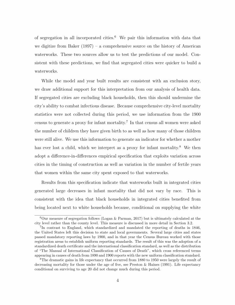
While the results are impressive, this public health movement would not have been

possible without earlier infrastructure investment. As Figure 1 illustrates, U.S. cities

built waterworks at a tremendous rate during the 1890s: by 1897 there were 3,167

waterworks in the United States with 83% built after 1880 and 46% built between

1890 and 1896.2 These investments, which occurred before effective water treatment

technologies existed, laid the necessary foundation for the elimination of infectious

waterborne diseases by connecting households to a centralized water supply. Without

these connections, future investments in water filtration would have been much less

effective at combatting waterborne disease, as residents with access to clean water

would remain at risk through their contact with residents without access.3

1On the role of waterborne diseases see (Cutler & Miller, 2005; Ferrie & Troesken, 2008; Alsan& Goldin, Forthcoming; Antman, 2015). For more on poor nutrition see (McKeown, 1976; Fogel,2004; Fogel & Costa, 1997). For air pollution see (Beach & Hanlon, Forthcoming; Clay et al., 2015).

2This statistic based on data from Baker (1897), the most comprehensive source on U.S. water-works. Section 3.1 describes this source in more detail.

3The waterborne disease Typhoid Fever, for instance, is typically spread through the consumptionof water that is tainted from the fecal waste of infected individuals. However, infection from other

1

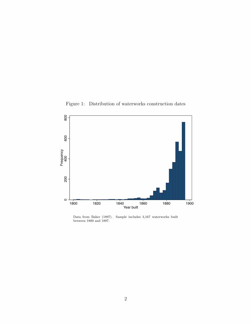
Figure 1: Distribution of waterworks construction dates

020

040

060

080

0Fr

eque

ncy

1800 1820 1840 1860 1880 1900Year built

Data from Baker (1897). Sample includes 3,167 waterworks builtbetween 1800 and 1897.

2

Given how closely these two movements are linked, it is surprising how little we

know about this initial wave of investment. Why American cities decided to build

when they did and what determines the extensiveness of the system that they built are

both open questions. These questions are also of central importance for understanding

the broader success of the movement to filter water and treat sewage. In light of this,

we ask whether the ability to exclude lower status groups played a role in shaping

investment decisions. Specifically, we examine the extent to which segregation of

black households influenced the timing of investment and, conditional on building a

waterworks, the overall extensiveness of the system.

Our motivation for considering the role of segregation stems is twofold. First,

the initial capital outlays for these waterworks were quite large: in 1890, the median

waterworks cost over $700,000 in 1890 dollars, comparable in cost to a $700,000,000

project for a modern city.4 Since these projects were financed at the local level,

investment likely depended on the political will of local residents. This brings us

to our second motivation. Since these investments were made before effective water

filtration and sewage treatment existed, taxpayers had little incentive to attempt to

internalize the future social returns that would be generated from universal access.5

We develop a theoretical model to illustrate how segregation might influence water

provision. We then draw on full count census data from 1880 to quantify the degree

forms of contact is also possible. The most well known example of this type of transmission isprobably “Typhoid Mary”, an asymptomatic carrier of typhoid who is presumed to have infectedover 50 people with typhoid fever during her career as a cook.

4Median waterworks cost is available from Baker (1897), although the figure we quote is basedon the incorporated cities that we use for our analysis. The modern project cost equivalent is basedon the economy cost of the project, the relative share of the project as a percent of total economyoutput, using the calculator at Measuring Worth.

5Cutler & Miller (2005) estimate the social rate of return on clean water technologies was greaterthan 23 to 1. This return only considers life expectancy gains, however, Beach et al. (2016) show thatearly-life exposure to waterborne disease impaired human capital development, affecting earningsand educational attainment. By helping eliminate this exposure, the authors estimate that the gainsto future income alone were enough to offset the costs of investment. Specifically, they estimate anadditional rate of return (relative to the cost of the building a waterworks) ranging from a low of 4to 1 to a high of 10 to 1.

3

of segregation in all incorporated cities.6 We pair this information with data that

we digitize from Baker (1897) – a comprehensive source on the history of American

waterworks. These two sources allow us to test the predictions of our model. Con-

sistent with these predictions, we find that segregated cities were quicker to build a

waterworks.

While the model and year built results are consistent with an exclusion story,

we draw additional support for this interpretation from our analysis of health data.

If segregated cities are excluding black households, then this should undermine the

city’s ability to combat infectious disease. Because comprehensive city-level mortality

statistics were not collected during this period, we use information from the 1900

census to generate a proxy for infant mortality.7 In that census all women were asked

the number of children they have given birth to as well as how many of those children

were still alive. We use this information to generate an indicator for whether a mother

has ever lost a child, which we interpret as a proxy for infant mortality.8 We then

adopt a difference-in-differences empirical specification that exploits variation across

cities in the timing of construction as well as variation in the number of fertile years

that women within the same city spent exposed to that waterworks.

Results from this specification indicate that waterworks built in integrated cities

generated large decreases in infant mortality that did not vary by race. This is

consistent with the idea that black households in integrated cities benefited from

being located next to white households because, conditional on supplying the white

6Our measure of segregation follows (Logan & Parman, 2017) but is ultimately calculated at thecity level rather than the county level. This measure is discussed in more detail in Section 3.2.

7In contrast to England, which standardized and mandated the reporting of deaths in 1846,the United States left this decision to state and local governments. Several large cities and statespassed mandatory reporting laws by 1900, and in that year the Census Bureau worked with thoseregistration areas to establish uniform reporting standards. The result of this was the adoption of astandardized death certificate and the international classification standard, as well as the distributionof “The Manual of International Classification of Causes of Death”, which cross referenced termsappearing in causes of death from 1890 and 1900 reports with the new uniform classification standard.

8The dramatic gains in life expectancy that occurred from 1880 to 1950 were largely the result ofdecreasing mortality for those under the age of five, see Preston & Haines (1991). Life expectancyconditional on surviving to age 20 did not change much during this period.

4

household with water, the marginal cost of supplying a black household with water

was very low. The health benefits of water investment, however, decline dramatically

as the level of segregation in the city increases. This is true for both white and black

households, which is consistent with the idea that by excluding black households

from the initial construction of waterworks, these cities were not able to effectively

eliminate waterborne diseases.

These results are largely complementary to previous work by Troesken (2002), on

which we extend in several ways. In that paper, Troesken posits that controlling wa-

terborne disease requires comprehensive access, which is more likely in an integrated

city rather than a segregated city. Troesken’s analysis, however, largely centers on

assessing the efficacy of the adoption of clean water technologies. Our paper, however,

is much more concerned with assessing the robustness of the link between segregation

and the extensiveness of a city’s waterworks. To this end, we formalize Troesken’s

intuition in order to generate a set of empirical predictions, which we subsequently

test empirically. A second point of differentiation is that, as a result of recently dig-

itized data, we are able to extend the scope of historical research on waterworks to

far more cities than previously possible. The recent release of the complete count

federal census data allows us to construct historical segregation estimates for every

city in the United States (Logan & Parman, 2017). Troesken, in contrast, was forced

to rely on a sample of 33 large cities because of the availability of both segregation

and mortality data. Our sample of over 1700 cities captures a much broader range of

city sizes, population compositions, and political environments.

5

2 Modeling the influence of segregation on local

water provision

Consider a city with two types of residents. For ease of exposition, we will define the

two groups as white and black residents; however, we could consider any minority

group that potentially faces discrimination in the provision of public goods. The city

lies on a unit interval with x = 0 being the whitest part of town and x = 1 being

the blackest. Without loss of generality, assume the city is one mile long. Each point

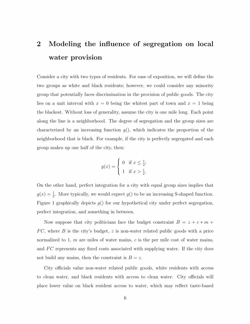
along the line is a neighborhood. The degree of segregation and the group sizes are

characterized by an increasing function g(), which indicates the proportion of the

neighborhood that is black. For example, if the city is perfectly segregated and each

group makes up one half of the city, then:

g(x) =

0 if x ≤ 12;

1 if x > 12.

On the other hand, perfect integration for a city with equal group sizes implies that

g(x) = 12. More typically, we would expect g() to be an increasing S-shaped function.

Figure 1 graphically depicts g() for our hypothetical city under perfect segregation,

perfect integration, and something in between.

Now suppose that city politicians face the budget constraint B = z + c ∗ m +

FC, where B is the city’s budget, z is non-water related public goods with a price

normalized to 1, m are miles of water mains, c is the per mile cost of water mains,

and FC represents any fixed costs associated with supplying water. If the city does

not build any mains, then the constraint is B = z.

City officials value non-water related public goods, white residents with access

to clean water, and black residents with access to clean water. City officials will

place lower value on black resident access to water, which may reflect taste-based

6

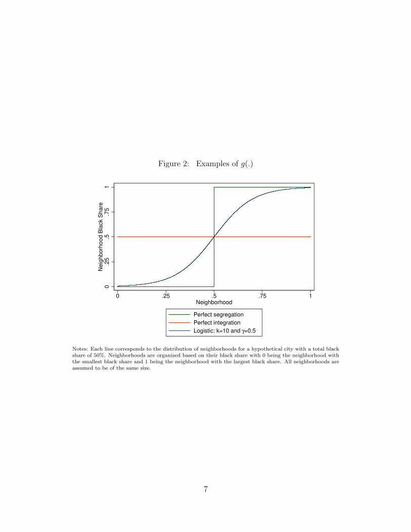
Figure 2: Examples of g(.)

0.2

5.5

.75

1N

eig

hborh

ood B

lack S

hare

0 .25 .5 .75 1Neighborhood

Perfect segregation

Perfect integration

Logistic: k=10 and γ=0.5

Notes: Each line corresponds to the distribution of neighborhoods for a hypothetical city with a total blackshare of 50%. Neighborhoods are organized based on their black share with 0 being the neighborhood withthe smallest black share and 1 being the neighborhood with the largest black share. All neighborhoods areassumed to be of the same size.

7

or statistical discrimination (e.g., the fact that black residents are more likely to be

disenfranchised and thus less likely to help keep city officials in office). Thus, if the

city builds a main, it will start at x = 0 (the whitest part of town), and keep building

the main, possibly stopping before supplying water to the whole city. If a main is

built to a particular neighborhood x, then both black and white residents of that

neighborhood have access to the main. Now let NW be the white population that is

connected to a water main, NB be the black population connected to a water main,

and m ∈ [0, 1] be where the city stops building the main. The variable m is the miles

of mains and a measure of the water system’s size. Then

NW =∫ m

0(1− g(x))dx (1)

NB =∫ m

0g(x)dx (2)

Now suppose the city’s utility function is:

U(NW , NB, Z) = αNW + (1− α)NB + βz (3)

where α ∈ (12, 1). The utility function in (Nw, Nb, z)-space is linear, but since g is

nonlinear, the utility function in (z,m)-space is non-linear.

For an interior solution, we need the ratio of marginal utilities of m and z to be

equal to the ratio of the costs of m and z. Since 1−αβ≤ MUm

MUz≤ α

β, an interior solution

will require that the per-mile cost c ∈(

1−αβ, αβ

). If c ≤ 1−α

β, then the city will provide

water to all residents. If c ≥ αβ, then the city will not provide water to any residents.

For an interior solution, taking the first-order conditions indicates that:

m∗ = g−1

(α− βc2α− 1

)(4)

Since g is an increasing function, it follows that g−1 is an increasing function.

8

Let λ = α−βc2α−1

. Then ∂λ∂c

= −β2α−1

< 0. Thus, an increase in the cost of a water

main decreases optimal main mileage. Similarly, an increase in the preferences for

non-water public goods decreases optimal main mileage. As for the preferences for

whites, ∂λ∂α

= 2βc−1(1−2α)2

, which is theoretically ambiguous.

Next, let’s characterize the function g to analyze the effects of segregation and

group size. Let

g(x) =1

1 + e−k(x−γ)(5)

This is an S-shaped curve in which k measures the degree of segregation. As k goes to

infinity, the city becomes perfectly segregated, while k = 0 implies perfect integration.

The parameter γ (the centering parameter) is the proportion of the city that is white.

Then,

g−1(x) = γ − 1

kln(

1

x− 1

). (6)

This implies that m∗ increases as white share increases. The effect of segregation on

water provision is ambiguous. If βc > 12, then segregation increases optimal main

mileage. If βc < 12, then segregation decreases optimal main mileage.

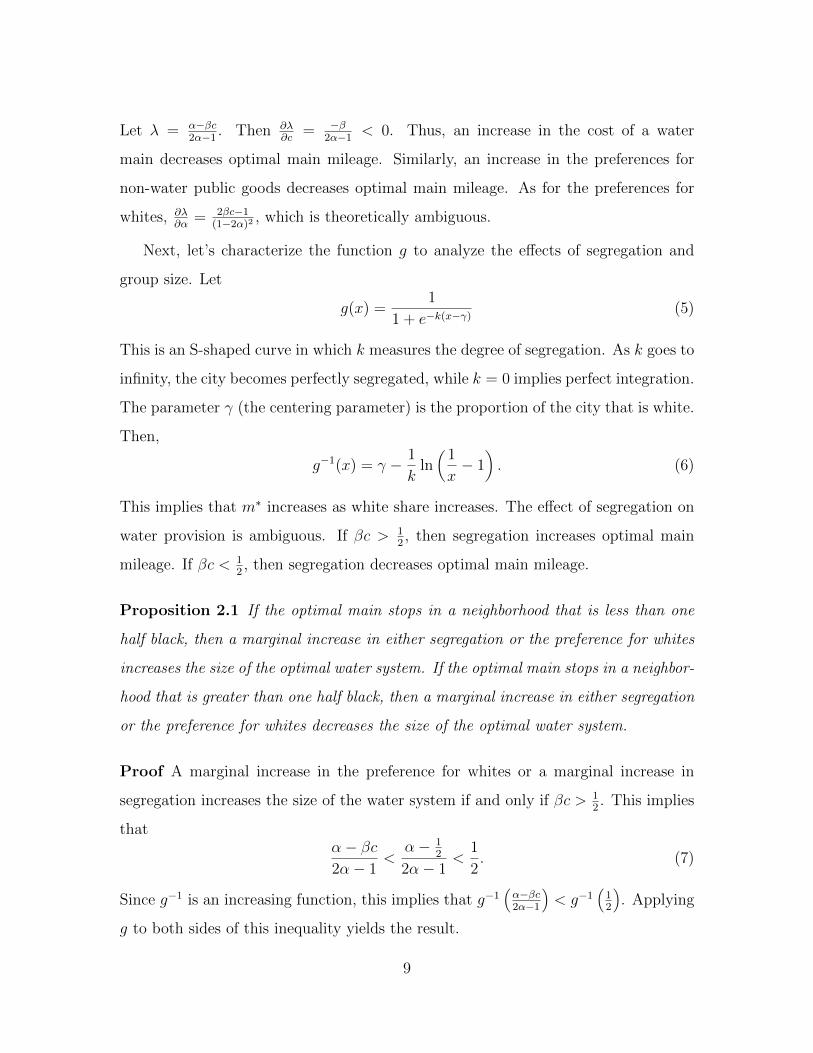
Proposition 2.1 If the optimal main stops in a neighborhood that is less than one

half black, then a marginal increase in either segregation or the preference for whites

increases the size of the optimal water system. If the optimal main stops in a neighbor-

hood that is greater than one half black, then a marginal increase in either segregation

or the preference for whites decreases the size of the optimal water system.

Proof A marginal increase in the preference for whites or a marginal increase in

segregation increases the size of the water system if and only if βc > 12. This implies

thatα− βc2α− 1

<α− 1

2

2α− 1<

1

2. (7)

Since g−1 is an increasing function, this implies that g−1(α−βc2α−1

)< g−1

(12

). Applying

g to both sides of this inequality yields the result.

9

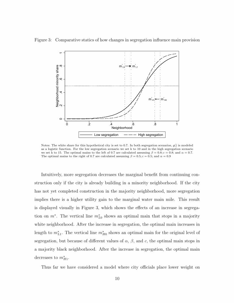
Figure 3: Comparative statics of how changes in segregation influence main provision

m*L0 m*

L1

m*H1 m*

H0

0.2

.4.6

.81

Nei

ghbo

rhoo

d m

inor

ity s

hare

0 .2 .4 .6 .8 1Neighborhood

Low segregation High segregation

Notes: The white share for this hypothetical city is set to 0.7. In both segregation scenarios, g() is modeledas a logistic function. For the low segregation scenario we set k to 10 and in the high segregation scenariowe set k to 15. The optimal mains to the left of 0.7 are calculated assuming β = 0.8; c = 0.8; and α = 0.7.The optimal mains to the right of 0.7 are calculated assuming β = 0.5; c = 0.5; and α = 0.9

Intuitively, more segregation decreases the marginal benefit from continuing con-

struction only if the city is already building in a minority neighborhood. If the city

has not yet completed construction in the majority neighborhood, more segregation

implies there is a higher utility gain to the marginal water main mile. This result

is displayed visually in Figure 3, which shows the effects of an increase in segrega-

tion on m∗. The vertical line m∗L0 shows an optimal main that stops in a majority

white neighborhood. After the increase in segregation, the optimal main increases in

length to m∗L1. The vertical line m∗

H0 shows an optimal main for the original level of

segregation, but because of different values of α, β, and c, the optimal main stops in

a majority black neighborhood. After the increase in segregation, the optimal main

decreases to m∗H1.

Thus far we have considered a model where city officials place lower weight on

10

black access to water. This is reflected in the preference parameter α, which can be

thought of as capturing local officials’ need to cater to likely voters, desire to focus

provision of public goods on those most able to finance those goods, or discrimina-

tory preferences for a particular group. Since roughly half of local waterworks were

privately owned during this period, a natural question is whether private provision

affects the predictions of our model. As private firms should be motivated by profits,

one would expect that private firms would not face the same pressure to discriminate.

In practice, however, private firms would still likely treat potential white and black

customers differently. In particular, if white residents have higher ability or willing-

ness to pay for water service on average, the firm’s profit function will effectively place

greater weight on neighborhoods with more white residents as those neighborhoods

would contain more paying customers and could thus be served with far lower average

costs per customer. Accordingly, private provision does not affect the comparative

statics of our model. These results are available in Appendix A.

3 Taking the model to the data

Our model of water provision leaves us with several testable predictions. First, the size

of the optimal water system increases with the size of the majority group. Second, in a

city in which the last water main stops in a neighborhood less than one half minority,

an increase in segregation should lead to an increase in the size of the optimal water

system. Third, in a city in which the last water main stops in a neighborhood more

than one half minority, an increase in segregation should lead to a decrease in the

size of the optimal water system.

The ideal dataset to examine these predictions would include: city-level variation

in black share, city-level variation in the segregation of the black population, and

high quality data that allows us to identify access to water and racial composition at

the neighborhood level. Our primary data constraint is that we are unaware of any

11

dataset that would allow us to take a comprehensive look at variation in access to

water at the neighborhood level. Instead, the bulk of our analysis will be conducted

at the city level.

3.1 Water provision data

Our primary source for information on water provision comes from the 1897 edition

of Moses Nelson Baker’s Manual of American Waterworks. Baker’s first volume of

the Manual of American Waterworks was published in 1888. As is made clear from

his introduction, Baker’s efforts were inspired by his frustration with the fact that

essential data on America’s waterworks (e.g., the number of waterworks, the location

of each waterworks, and when each waterworks was built) were not accurately known.

Baker attempted to remedy this situation by surveying local officials and companies

to obtain accurate histories and continuing to follow up with these individuals until he

received the requested information. Subsequent editions focused on standardizing the

information obtained from those surveys so that the information could be included in

future editions. Baker also incorporated information on works built since the initial

survey. For these reasons, we focus on digitizing the 1897 edition of the manual as it

is the most comprehensive of the four volumes.

For each waterworks, the manual includes information on “its history, general

character, the capacity of the pumps, reservoirs, stand-pipes, or filters; the extent of

the distribution system; and the most important figures relating to the finances of each

system” (Baker (1897), preface). A representative example of one these descriptions

is provided in Figure 4. The main piece of information we focus on is the year the

waterworks was built. We digitize this information for all 4,207 cities appearing in

the 1897 manual.

It is worth pointing out why we prefer to use year built instead of other mea-

sures, such as miles of mains or number of taps, which relate directly to the measures

12

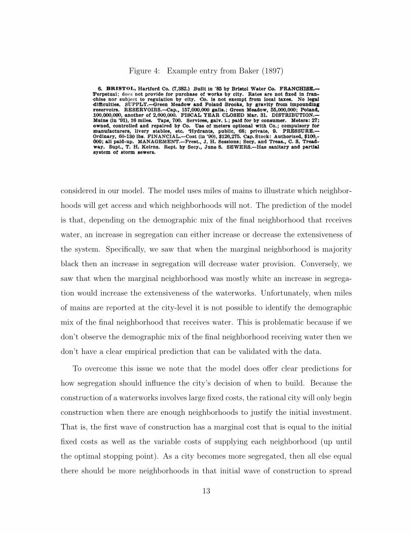
Figure 4: Example entry from Baker (1897)

considered in our model. The model uses miles of mains to illustrate which neighbor-

hoods will get access and which neighborhoods will not. The prediction of the model

is that, depending on the demographic mix of the final neighborhood that receives

water, an increase in segregation can either increase or decrease the extensiveness of

the system. Specifically, we saw that when the marginal neighborhood is majority

black then an increase in segregation will decrease water provision. Conversely, we

saw that when the marginal neighborhood was mostly white an increase in segrega-

tion would increase the extensiveness of the waterworks. Unfortunately, when miles

of mains are reported at the city-level it is not possible to identify the demographic

mix of the final neighborhood that receives water. This is problematic because if we

don’t observe the demographic mix of the final neighborhood receiving water then we

don’t have a clear empirical prediction that can be validated with the data.

To overcome this issue we note that the model does offer clear predictions for

how segregation should influence the city’s decision of when to build. Because the

construction of a waterworks involves large fixed costs, the rational city will only begin

construction when there are enough neighborhoods to justify the initial investment.

That is, the first wave of construction has a marginal cost that is equal to the initial

fixed costs as well as the variable costs of supplying each neighborhood (up until

the optimal stopping point). As a city becomes more segregated, then all else equal

there should be more neighborhoods in that initial wave of construction to spread

13

those fixed costs across. As a result, more segregated cities should begin construction

earlier than integrated cities.

3.2 Demographic data

With our empirical prediction in hand, we now set out to attach demographic charac-

teristics to our waterworks data. Our demographic data come from the complete count

1880 census as maintained by the Integrated Public Use Microdata Series (IPUMS)

(Ruggles et al., 2015). We rely on this dataset to identify: number of households

residing in the city, the black share, and the level of segregation in the city. We

begin with the sample of individuals residing in an incorporated place in 1880. By

using incorporated places we are not restricted to the sample of large cities that are

typically reported in census publications, but are instead able to obtain demographic

data for roughly 5,400 cities and villages.

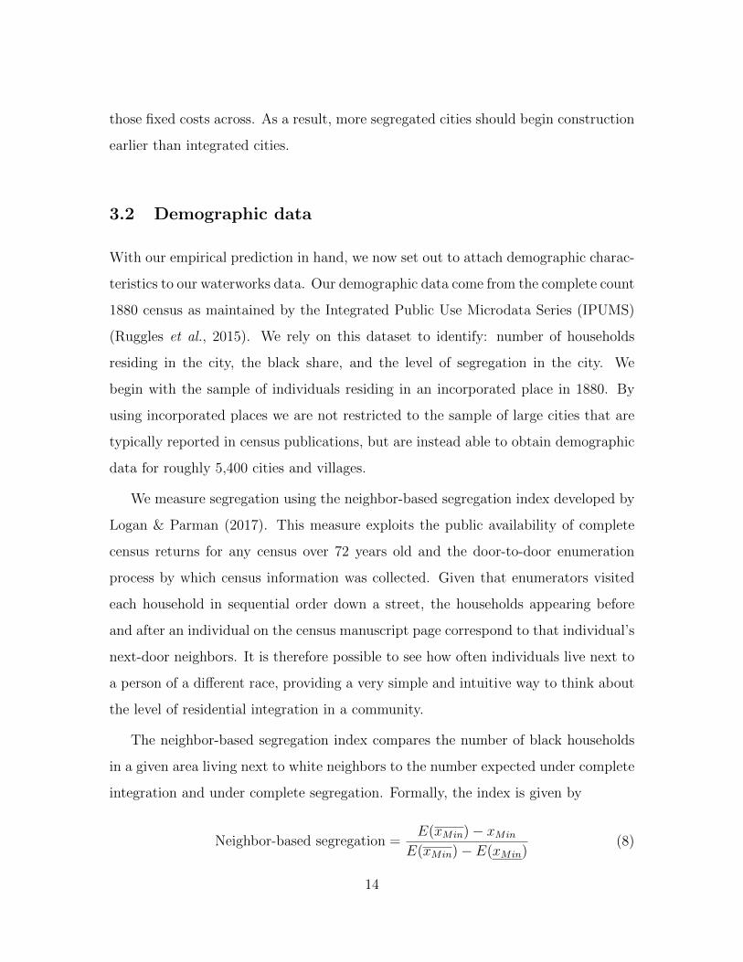
We measure segregation using the neighbor-based segregation index developed by

Logan & Parman (2017). This measure exploits the public availability of complete

census returns for any census over 72 years old and the door-to-door enumeration

process by which census information was collected. Given that enumerators visited

each household in sequential order down a street, the households appearing before

and after an individual on the census manuscript page correspond to that individual’s

next-door neighbors. It is therefore possible to see how often individuals live next to

a person of a different race, providing a very simple and intuitive way to think about

the level of residential integration in a community.

The neighbor-based segregation index compares the number of black households

in a given area living next to white neighbors to the number expected under complete

integration and under complete segregation. Formally, the index is given by

Neighbor-based segregation =E(xMin)− xMin

E(xMin)− E(xMin)(8)

14

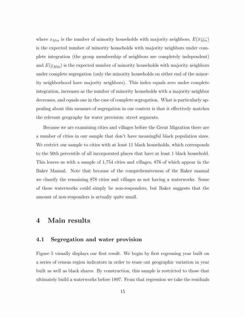
where xMin is the number of minority households with majority neighbors, E(xMin)

is the expected number of minority households with majority neighbors under com-

plete integration (the group membership of neighbors are completely independent)

and E(xMin) is the expected number of minority households with majority neighbors

under complete segregation (only the minority households on either end of the minor-

ity neighborhood have majority neighbors). This index equals zero under complete

integration, increases as the number of minority households with a majority neighbor

decreases, and equals one in the case of complete segregation. What is particularly ap-

pealing about this measure of segregation in our context is that it effectively matches

the relevant geography for water provision: street segments.

Because we are examining cities and villages before the Great Migration there are

a number of cities in our sample that don’t have meaningful black population sizes.

We restrict our sample to cities with at least 11 black households, which corresponds

to the 50th percentile of all incorporated places that have at least 1 black household.

This leaves us with a sample of 1,754 cities and villages, 876 of which appear in the

Baker Manual. Note that because of the comprehensiveness of the Baker manual

we classify the remaining 878 cities and villages as not having a waterworks. Some

of these waterworks could simply be non-responders, but Baker suggests that the

amount of non-responders is actually quite small.

4 Main results

4.1 Segregation and water provision

Figure 5 visually displays our first result. We begin by first regressing year built on

a series of census region indicators in order to tease out geographic variation in year

built as well as black shares. By construction, this sample is restricted to those that

ultimately build a waterworks before 1897. From that regression we take the residuals

15

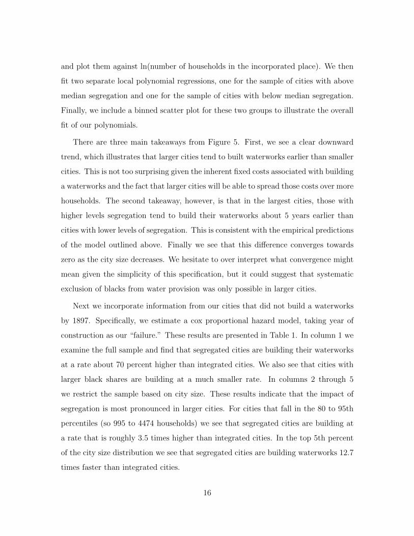
and plot them against ln(number of households in the incorporated place). We then

fit two separate local polynomial regressions, one for the sample of cities with above

median segregation and one for the sample of cities with below median segregation.

Finally, we include a binned scatter plot for these two groups to illustrate the overall

fit of our polynomials.

There are three main takeaways from Figure 5. First, we see a clear downward

trend, which illustrates that larger cities tend to built waterworks earlier than smaller

cities. This is not too surprising given the inherent fixed costs associated with building

a waterworks and the fact that larger cities will be able to spread those costs over more

households. The second takeaway, however, is that in the largest cities, those with

higher levels segregation tend to build their waterworks about 5 years earlier than

cities with lower levels of segregation. This is consistent with the empirical predictions

of the model outlined above. Finally we see that this difference converges towards

zero as the city size decreases. We hesitate to over interpret what convergence might

mean given the simplicity of this specification, but it could suggest that systematic

exclusion of blacks from water provision was only possible in larger cities.

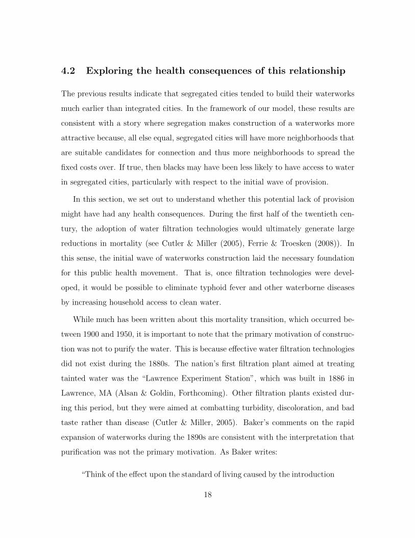
Next we incorporate information from our cities that did not build a waterworks

by 1897. Specifically, we estimate a cox proportional hazard model, taking year of

construction as our “failure.” These results are presented in Table 1. In column 1 we

examine the full sample and find that segregated cities are building their waterworks

at a rate about 70 percent higher than integrated cities. We also see that cities with

larger black shares are building at a much smaller rate. In columns 2 through 5

we restrict the sample based on city size. These results indicate that the impact of

segregation is most pronounced in larger cities. For cities that fall in the 80 to 95th

percentiles (so 995 to 4474 households) we see that segregated cities are building at

a rate that is roughly 3.5 times higher than integrated cities. In the top 5th percent

of the city size distribution we see that segregated cities are building waterworks 12.7

times faster than integrated cities.

16

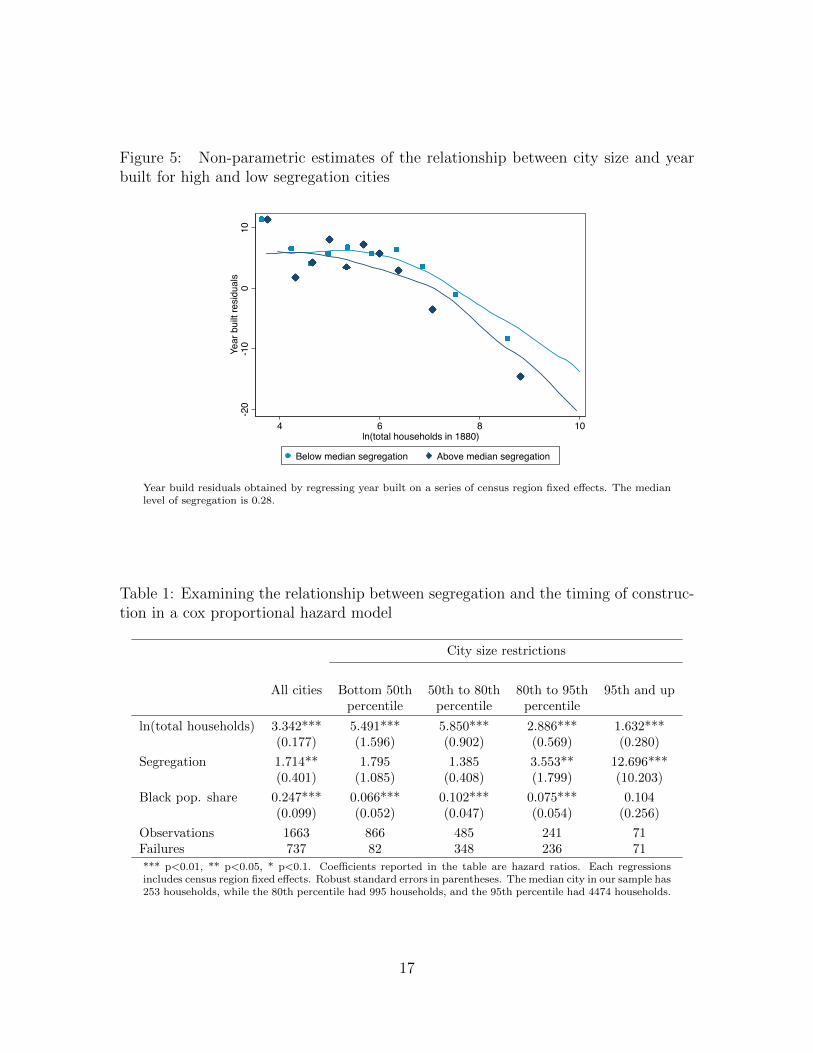
Figure 5: Non-parametric estimates of the relationship between city size and yearbuilt for high and low segregation cities

-20

-10

010

Year

bui

lt re

sidu

als

4 6 8 10ln(total households in 1880)

Below median segregation Above median segregation

Year build residuals obtained by regressing year built on a series of census region fixed effects. The medianlevel of segregation is 0.28.

Table 1: Examining the relationship between segregation and the timing of construc-tion in a cox proportional hazard model

City size restrictions

All cities Bottom 50th 50th to 80th 80th to 95th 95th and uppercentile percentile percentile

ln(total households) 3.342*** 5.491*** 5.850*** 2.886*** 1.632***(0.177) (1.596) (0.902) (0.569) (0.280)

Segregation 1.714** 1.795 1.385 3.553** 12.696***(0.401) (1.085) (0.408) (1.799) (10.203)

Black pop. share 0.247*** 0.066*** 0.102*** 0.075*** 0.104(0.099) (0.052) (0.047) (0.054) (0.256)

Observations 1663 866 485 241 71Failures 737 82 348 236 71

*** p<0.01, ** p<0.05, * p<0.1. Coefficients reported in the table are hazard ratios. Each regressionsincludes census region fixed effects. Robust standard errors in parentheses. The median city in our sample has253 households, while the 80th percentile had 995 households, and the 95th percentile had 4474 households.

17

4.2 Exploring the health consequences of this relationship

The previous results indicate that segregated cities tended to build their waterworks

much earlier than integrated cities. In the framework of our model, these results are

consistent with a story where segregation makes construction of a waterworks more

attractive because, all else equal, segregated cities will have more neighborhoods that

are suitable candidates for connection and thus more neighborhoods to spread the

fixed costs over. If true, then blacks may have been less likely to have access to water

in segregated cities, particularly with respect to the initial wave of provision.

In this section, we set out to understand whether this potential lack of provision

might have had any health consequences. During the first half of the twentieth cen-

tury, the adoption of water filtration technologies would ultimately generate large

reductions in mortality (see Cutler & Miller (2005), Ferrie & Troesken (2008)). In

this sense, the initial wave of waterworks construction laid the necessary foundation

for this public health movement. That is, once filtration technologies were devel-

oped, it would be possible to eliminate typhoid fever and other waterborne diseases

by increasing household access to clean water.

While much has been written about this mortality transition, which occurred be-

tween 1900 and 1950, it is important to note that the primary motivation of construc-

tion was not to purify the water. This is because effective water filtration technologies

did not exist during the 1880s. The nation’s first filtration plant aimed at treating

tainted water was the “Lawrence Experiment Station”, which was built in 1886 in

Lawrence, MA (Alsan & Goldin, Forthcoming). Other filtration plants existed dur-

ing this period, but they were aimed at combatting turbidity, discoloration, and bad

taste rather than disease (Cutler & Miller, 2005). Baker’s comments on the rapid

expansion of waterworks during the 1890s are consistent with the interpretation that

purification was not the primary motivation. As Baker writes:

“Think of the effect upon the standard of living caused by the introduction

18

of a public water supply! In place of the labor attendant upon lifting water

by the old oaken bucket, the more prosaic hand pump, or of carrying

water in pails from some spring or stream, only a turn of the faucet is

now necessary in hundreds of communities to secure either hot or cold

water on any floor of a dwelling. The labor saving thus secured, together

with the increase in convenience, comfort and cleanliness, is too evident to

need detailed mention, especially as both the old and the new are within

the experiences of so many.”

Largely due to the technological constraints of the time, initial water investment

decisions were motivated by convenience rather than the control of disease. The

systematic exclusion of blacks makes much more sense when the goal is to increase

convenience rather than when the goal is to combat disease. When the goal is to

combat disease, there is a stronger motivation to increase black household’s access

to water. Humans can be carriers of waterborne diseases like typhoid fever, and so

black households without access to clean water may still contract the disease and

spread it to white households. In the context of our model, local officials interested

in combating typhoid fever and other waterborne diseases may value black household

and white household access equally (α = 0.5), which would undermine any empiri-

cal predictions about how segregation should affect the city’s overall health. When

investment decisions are motivated by convenience, however, it is much more likely

that local officials will undervalue black access. This is important because it suggests

that α > 0.5, and so we should expect the level of segregation in the city to generate

variation in black vs. white household provision.

While purification was not the primary motivation, for many cities the construc-

tion of a waterworks allowed residents to access water sources that were less likely

to be tainted by improper sewage disposal, thus limiting exposure to waterborne dis-

eases (see, for instance, Alsan & Goldin (Forthcoming) on water and sewerage access

in Massachusetts). This, combined with the fact that initial provision decisions were

19

motivated by convenience rather than disease, generates the following empirical pre-

diction. In an integrated city, the construction of a waterworks will provide black

and white households with better access to clean water, which will in turn is likely

to lower the incidence of waterborne disease. In a segregated city, however, blacks

are more likely to be excluded from access to clean water, which will undermine the

city’s ability to control waterborne diseases like typhoid fever.

To test this empirical prediction, we draw on data from the IPUMS 5% sample

of the 1900 census. In that census, each woman was asked about how many children

they have had and how many of those children are still living today. As in Logan &

Parman (2018), we use this information to construct an indicator variable for whether

an individual ever lost a child, which we interpret as a proxy for infant mortality. We

rely on this proxy because comprehensive city-level data on black and white mortality

by age and cause does not exist for this time period.9

Figure 6 displays our main result with raw data. Specifically, we plot our indicator

for losing a child against city-level segregation. We plot this relationship separately

for white mothers (left panel) and black mothers (right panel). We also plot the

relationship separately for those who were less than the age of 18 when the water-

works was constructed and those who were over the age of 45 when the waterworks

constructed. We interpret those who were under the age of 18 as those who spent

all of their fertile years in the regime where the city was providing its residents with

water. Conversely, we interpret those were over the age of 45 as those who spent all

of their fertile years without a waterworks.

9In contrast to England, which standardized and mandated the reporting of deaths in 1846,the United States left this decision to state and local governments. Several large cities and statespassed mandatory reporting laws by 1900, and in that year the Census Bureau worked with thoseregistration areas to establish uniform reporting standards. The result of this was the adoption ofa standardized death certificate and the international classification standard, as well as the distri-bution of “The Manual of International Classification of Causes of Death”, which cross referencedterms appearing in causes of death from 1890 and 1900 reports with the new uniform classifica-tion standard. While the registration area would expand dramatically over the next 30 years, thecity-level tabulations simply do not include the necessary detail for our analysis.

20

The results of Figure 6 are as follows. In an integrated city, the share of mothers

that lost a child is about 5 percentage points lower for mothers who spent their

fertile years in a city with a waterworks vs mothers who spend their fertile years in

a city without a waterworks. Notably, this decline is roughly the same size for both

black and white mothers, which is consistent with black households gaining access to

water at the same rate that white households are gaining access to water. However,

we also see that these benefits decline as the level of segregation increases, which is

consistent with the exclusion of black households hindering the city’s ability to control

waterborne disease rates.

Next we analyze this relationship in a formal difference-in-differences specification.

Specifically we estimate variations of the following equation:

Lostiac = α0 + βa + γc + δ ∗ Exposureiac + ψ ∗White+ εiac (9)

where Lostiac is an indicator that equals 1 if individual i, who is age a and resides in cit

c at the time of census enumeration has ever lost a child. The parameters βa and γc are

age and city fixed effects, respectively. The variable Exposureiac captures the share of

fertile years (ages 18-45) that the individual spent in a city with water access. This is

calculated by taking the individual’s age at the time of enumeration and backing out

how old they would have been at the time the waterworks was built. If the individual

was under the age of 18 when the waterworks is built then they are assigned a 1. If

the individual was 45 or older then they are assigned zero. The remaining individuals

receive partial exposure corresponding to 45−age at time of construction45−20

. Finally, we include

an indicator for whether the individual is white or not since black and white mothers

lost children at different rates. In some specifications we will interact our exposure

variable by race and by the degree of segregation in the city. Standard errors are

clustered at the city level. Identification of δ comes from the fact that different cities

built their waterworks at different times and that, within a city, the construction of a

21

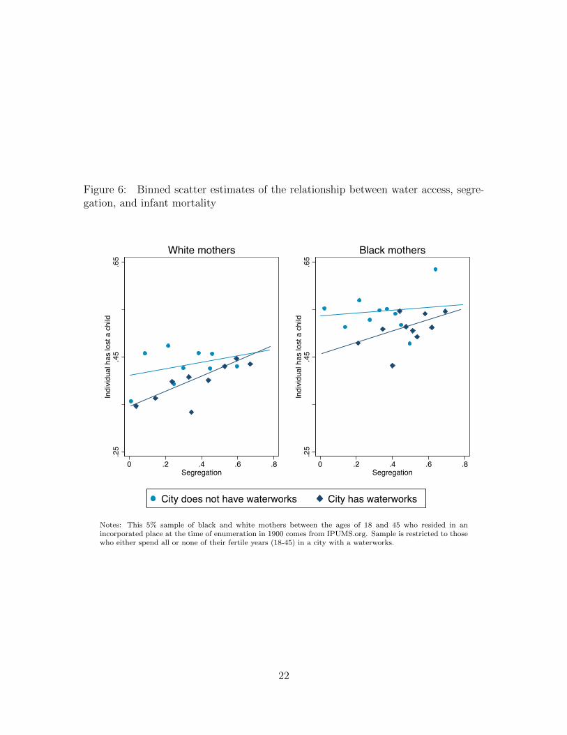
Figure 6: Binned scatter estimates of the relationship between water access, segre-gation, and infant mortality

.25

.45

.65

Indi

vidu

al h

as lo

st a

chi

ld

0 .2 .4 .6 .8Segregation

White mothers

.25

.45

.65

Indi

vidu

al h

as lo

st a

chi

ld

0 .2 .4 .6 .8Segregation

Black mothers

City does not have waterworks City has waterworks

Notes: This 5% sample of black and white mothers between the ages of 18 and 45 who resided in anincorporated place at the time of enumeration in 1900 comes from IPUMS.org. Sample is restricted to thosewho either spend all or none of their fertile years (18-45) in a city with a waterworks.

22

waterworks generates differential exposure to water access based on the individual’s

age when the waterworks was built.

Column 1 of Table 2 presents estimates of equation 9. In this specification we

find that investment in water decreased the likelihood of losing a child by roughly 4

percentage points, which is broadly similar with the results depicted in Figure 6. Note

that our estimating equation includes city fixed effects, which absorbs the average

effects of segregation, city size, and year built. In column 2 we interact our exposure

variable with an indicator for whether the mother is black. Here we see little evidence

that water investments differentially benefit white households. In column 3 we include

an interaction with our segregation variable. In this specification, “Water Exposure”

is interpreted as the effect of building a waterworks in an integrated city. There we see

that the likelihood of losing a child fell by roughly 10 percentage points for mothers

that spent their entire fertile years in a city that had a waterworks and that the

degree of segregation in the city mitigates this effect. This effect is both practically

and statistically significant such that moving from perfect integration to a segregation

index of 0.5 generates no measurable decline in infant mortality. In column 4 we

fully interact both “Water Exposure” and “Water Exposure × Segregation” with an

indicator for whether the mother is black. Again, we cannot reject that the effect for

white mothers is different from the effect for black mothers.

23

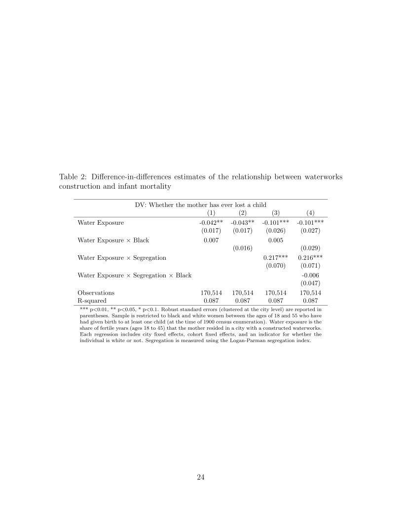
Table 2: Difference-in-differences estimates of the relationship between waterworksconstruction and infant mortality

DV: Whether the mother has ever lost a child(1) (2) (3) (4)

Water Exposure -0.042** -0.043** -0.101*** -0.101***(0.017) (0.017) (0.026) (0.027)

Water Exposure × Black 0.007 0.005(0.016) (0.029)

Water Exposure × Segregation 0.217*** 0.216***(0.070) (0.071)

Water Exposure × Segregation × Black -0.006(0.047)

Observations 170,514 170,514 170,514 170,514R-squared 0.087 0.087 0.087 0.087

*** p<0.01, ** p<0.05, * p<0.1. Robust standard errors (clustered at the city level) are reported inparentheses. Sample is restricted to black and white women between the ages of 18 and 55 who havehad given birth to at least one child (at the time of 1900 census enumeration). Water exposure is theshare of fertile years (ages 18 to 45) that the mother resided in a city with a constructed waterworks.Each regression includes city fixed effects, cohort fixed effects, and an indicator for whether theindividual is white or not. Segregation is measured using the Logan-Parman segregation index.

24

5 Concluding remarks

During the first half of the twentieth century, the United States experienced a dra-

matic decline in mortality as cities invested in clean water technologies. However, this

public health movement would not have been possible without prior infrastructure in-

vestment, which connected households to a centralized water supply. In this paper, we

ask whether the segregation of blacks might have influenced municipal investments,

and in turn influenced this public health movement. We find evidence consistent with

the narrative that segregated cities were quicker to build their waterworks and more

likely to exclude households. This exclusion may not have been rational, however, as

we also find that segregated cities experienced much smaller declines in infant mor-

tality, perhaps because by excluding black households they were unable to effectively

control waterborne disease.

References

Alsan, Marcella, & Goldin, Claudia. Forthcoming. Watersheds in infant mortality: The role of

effective water and sewerage infrastructure, 1880 to 1915. Journal of Political Economy.

Antman, Francisca M. 2015. For want of a cup: The rise of tea in England and the impact of water

quality on economic development. Tech. rept. Mimeo.

Baker, Moses Nelson. 1897. The manual of American water-works. Vol. 4. Engineering News.

Beach, Brian, & Hanlon, W. Walker. Forthcoming. Coal smoke and mortality in an early industrial

economy. The Economic Journal.

Beach, Brian, Ferrie, Joseph, Saavedra, Martin, & Troesken, Werner. 2016. Typhoid fever, water

quality, and human capital formation. Journal of Economic History, 76(01), 41–75.

Cain, Louis, & Hong, Sok Chul. 2009. Survival in 19th century cities: The larger the city, the smaller

your chances. Explorations in Economic History, 46(4), 450–463.

Clay, Karen, Lewis, Joshua, & Severnini, Edson. 2015. Canary in a Coal Mine: Impact of Mid-20th

Century Air Pollution Induced by Coal-Fired Power Generation on Infant Mortality and Property

Values. Tech. rept. Working paper.

25

Cutler, David, & Miller, Grant. 2005. The role of public health improvements in health advances:

The twentieth-century United States. Demography, 42(1), 1–22.

Ferrie, Joseph P, & Troesken, Werner. 2008. Water and Chicagos mortality transition, 1850–1925.

Explorations in Economic History, 45(1), 1–16.

Fogel, Robert W, & Costa, Dora L. 1997. A theory of technophysio evolution, with some implications

for forecasting population, health care costs, and pension costs. Demography, 34(1), 49–66.

Fogel, Robert William. 2004. The escape from hunger and premature death, 1700-2100: Europe,

America, and the Third World. Vol. 38. Cambridge University Press.

Kesztenbaum, Lionel, & Rosenthal, Jean-Laurent. 2011. The health cost of living in a city: The

case of France at the end of the 19th century. Explorations in Economic History, 48(2), 207–225.

Logan, Trevon D, & Parman, John M. 2017. The national rise in residential segregation. Journal of

Economic History, 77(1), 127–170.

Logan, Trevon D, & Parman, John M. 2018. Segregation and mortality over time and space. Social

Science & Medicine, 199, 77–86.

McKeown, Thomas. 1976. The modern rise of population.

Preston, Samuel H, & Haines, Michael R. 1991. Fatal years: Child mortality in late nineteenth-

century America. Vol. 1175. Princeton University Press.

Ruggles, Steven, Genadek, Katie, Goeken, Ronald, Grover, Josiah, & Sobek, Matthew. 2015. Inte-

grated Public Use Microdata Series: Version 6.0 [dataset]. Minneapolis: University of Minnesota.

http://doi.org/10.18128/D010.V6.0.

Troesken, Werner. 2002. The limits of Jim Crow: race and the provision of water and sewerage

services in American cities, 1880–1925. Journal of Economic History, 62(03), 734–772.

26

A Extending the model

A.1 Private provision without price discrimination

Suppose that the city is on a unit interval and the degree of segregation is described

by the g function from the previous subsection. However, instead of public officials

deciding water provision, suppose water is provided by a profit maximizing firm. The

profit maximizing firm must decide what price to charge and how many miles of mains

to build. Assume the firm cannot price discriminate, and must charge a single price

for connecting to the water system. Further assume that all whites are willing to pay

δ to connect to the water system, whereas all blacks are willing to pay θ, and that

δ > θ. Since whites are willing to pay more, the firm will start construction of the

mains in the whitest part of town, indexed by 0 on the unit interval.

The firm will either charge δ or θ to hook up to the water system. If the price were

set below δ and above θ, then the firm could raise prices without losing any customers;

the firm would never charge below θ because it is the minimum willingness to pay in

the model. If the firm charges δ, then profits are

Πδ = δ∫ m

0(1− g(x))dx− pm− C, (10)

where m is the miles of mains, p is the per unit cost of mains, C is the fixed cost of

building the mains. The first order condition yields:

m∗ = g−1(

1− p

δ

). (11)

This implies that miles of mains decrease as the price per main increases and that

miles of mains increases as the willingness of whites to pay increases. Furthermore,

mains increase with the share of whites. Segregation decreases water provision if the

27

mark up is sufficiently low (2p > δ). This is because if the mark up is low, then the

private firm will stop constructing mains when it reaches the black neighborhood.

If the mark up is sufficiently high, however, it will be worth constructing mains in

the black neighborhoods to reach the few white customers that do exist. For this

equilibrium, only whites connect to the water system.

The second possible price strategy is if the firm charges θ so that both black and

white customers connect to the main. In this case,

Πθ = θm− pm− C (12)

So long as the price per unit of main is smaller than θ, this will give us a corner

solution of providing water to the whole city. In this equilibrium, the firm is already

covering the whole city and segregation and the share of whites have no effect on

main mileage.

Letting m∗δ be the optimal miles of main under the δ pricing strategy, then the

firm will pick the δ pricing strategy so long as:

δ∫ m∗

δ

0(1− g(x)) dx− θ > pm∗

δ − p. (13)

Of course fixed cost must be sufficiently small so that profits are non-negative.

A.2 Private provision with price discrimination

Now suppose the firm can price discriminate, so that the firm charges all blacks θ and

all whites δ so long as the firm builds a main to that particular neighborhood. Then

profits become:

Π = δ∫ m

0(1− g(x))dx+ θ

∫ m

0g(x)− pm− C (14)

28

The first order conditions give us that:

m∗ = g−1

(δ − pδ − θ

)(15)

Therefore, mileage of mains decreases with costs p. The comparative statics reveal

that mileage increases with the WTP of whites if the costs per unit is greater than the

WTP of blacks (p > θ). Notice that if p > θ, then whites are effectively subsidizing

blacks. In the absence of whites in the neighborhood, building in the black neigh-

borhood would not be profitable. An increase in the WTP of blacks increases main

mileage so long as δ > p, which is necessary for the water provision to be profitable.

Water provision increases with the share of whites γ. An increase in segregation in-

creases water provision so long as δ−θ > 2(δ−p) (or, alternatively, 2p > δ−θ), which

is to say if WTP of whites over blacks is at least twice as large as the mark up for

whites. This result is similar to the role of segregation without price discrimination.

In the case of no price discrimination, if the mark up for whites is high (2p > δ), it

is worth extending mains to neighborhoods with even a small number of whites. In

the case of price discrimination, this logic still holds except except that the threshold

is lower given that the firm receives revenues from the black households (2p must be

greater than δ − θ rather than just δ).

29