Segment Good

7/30/2019 Segment Good

http://slidepdf.com/reader/full/segment-good 1/11

Image Segmentation

Segmentation

• Subdivide an image into regions or objects

– Convert an image into a representation that is more meaningful and easier to analyze

– Assign a label to every pixel such that pixels with the same label share certain visual characteristics

– One of the most difficult tasks in image processing

∗ May be simplified by use of sensors for specific applications

∗ IR sensor to detect heat signatures of objects

• Applications include

– Medical imaging (locating tumors, studying anatomical structures)

– Region classification in satellite images

– Detection of disease in crops

– Machine vision for industrial inspection

• Algorithms based on basic properties of intensity values: discontinuity and similarity

– Discontinuity

∗ Partition an image based on abrupt changes in intensity values, such as edges

∗ Boundaries of regions are sufficiently different from each other and from the background

– Similarity

∗ Partition an image into regions that are similar according to some predefined criteria

Fundamentals

• Let R be the spatial region occupied by an image

• Image segmentation is the process that partitions R into n subregions R1, R2, . . . , Rn such that

1.ni=1 Ri = R

2. Ri is a connected set, i = 1, 2, . . . , n

3. Ri ∩ Rj = ∅ ∀i,j,i = j

4. Q(Ri) = true for i = 1, 2, . . . , n

5. Q(Ri ∪ Rj) = false for any adjacent region Ri and Rj

– Q(Rk) is a logical predicate defined over the points in set Rk

– Two regions Ri and Rj are said to be adjacent if their union forms a connnected set

• Figure 10.1

Thresholding

• Simplest method for image segmentation

• Based on a threshold value to turn a grayscale image into a binary image

• Highly dependent on selection of the threshold value



Image Segmentation 2

Point, line, and edge detection

• Detection of sharp, local changes in intensity

• Interested in isolated points, lines, and edges

• Edge pixels

– pixels at which the intensity of an image function changes abruptly

• Edges

– Sets of connected edge pixels

• Edge detectors

– Local image processing methods designed to detect edge pixels

• Line

– An edge segment in which intensity of the background on either side of the line is much higher or much lower than

the intensity of line pixels

• Isolated point

– A line with length and width equal to one pixel

• Background

– Local averaging smooths an image

– Since averaging is same as integration, abrupt changes can be detected by differentiation, using first- and second-

order derivatives

– Derivatives of a digital function

∗Computed in terms of differences in neighboring pixels

∗ Approximation used for a first derivative

1. Must be zero in areas of constant intensity

2. Must be nonzero at the onset of an intensity step or ramp

3. Must be nonzero at points along an intensity ramp

∗ Approximation used for a second derivative

1. Must be zero in areas of constant intensity

2. Must be nonzero at the onset and end of an intensity step or ramp

3. Must be zero along intensity ramps

∗ The maximum possible intensity change for digital [finite] quantities is also finite

∗ Shortest distance over which a change can occur is adjacent pixels

– Approximation to the first-order derivative at point x of a 1D function f (x)∗ Expand the function f (x + ∆x) into a Taylor series about x

∗ Let ∆x = 1

∗ Keep only the digital terms

∂f

∂x= f (x) = f (x + 1) − f (x)




– Second derivative is computed by differentiating the first derivative

∂ 2f

∂x2=

∂f (x)

∂x= f (x + 1) − f (x)

= (f (x + 2)

−f (x + 1))

−(f (x + 1)

−f (x))

= f (x + 2) − 2f (x + 1) + f (x)

∗ This expression is about point x + 1

∗ Translate it to point x to get

∂ 2f

∂x2= f (x) = f (x + 1) + f (x − 1) − 2f (x)

– Verify that the expressions for first- and second-order derivatives satisfy the conditions outlined

– Figure 10.2

∗ First-order derivative is nonzero at the onset and along the entire intensity ramp, producing thick edges

∗ Second-order derivative is nonzero only at the onset and end of ramp, producing finer edges

∗ For isolated noise point, second-order derivative has a much stronger response compared to the first-orderderivative

· Second-order derivative is much more aggressive than first-order derivative in enhancing sharp changes

· Second-order derivative enhances fine detail (including noise) much more than the first-order derivative

∗ In both ramp and step edges, second-order derivative has opposite signs as it transitions into and out of an edge

· The double-edge effect is used to locate edges

– Summary of observations

1. First-order derivatives produce thicker edges in an image

2. Second-order derivatives have a stronger response to fine detail, such as thin lines, isolated points, and noise

3. Second-order derivatives produce a double-edged response at ramp and step transitions in intensity

4. Sign of second derivative can be used to determine whether the transition into an edge is from light to dark or

dark to light– Use spatial filters [convolution kernels] to compute first and second derivatives at every pixel location

∗ Response of filter at center point of a 3 × 3 region is

R = w1z1 + w2z2 + · · · + w9z9

=

9k=1

wkzk

∗ Spatial filter mask given by

w1 w2 w3

w4 w5 w6

w7 w8 w9

• Detection of isolated points

– Based on second derivative using the Laplacian

∇2f (x, y) =∂ 2f

∂x2+

∂ 2f

∂y2

– Partials are given by

∂ 2f (x, y)

∂x2= f (x + 1, y) + f (x − 1, y) − 2f (x, y)

= f (x, y + 1) + f (x, y − 1) − 2f (x, y)




– Laplacian is given by

∇2f (x, y) = f (x + 1, y) + f (x − 1, y) + f (x, y + 1) + f (x, y − 1) − 4f (x, y)

– Implemented by a 4-neighborhood mask, or can be extended to an 8-neighborhood mask

– Figure 10.4

∗ Select a point in the output image if its response to the mask exceeds a specified threshold; deselect others

g(x, y) =

1 if |R(x, y)| ≥ T 0 otherwise

– Note that in constant intensity areas, the mask response will be zero

• Line detection

– Second derivative results in a stronger response and produces thinner lines compared to first derivative

∗ Use Laplacian mask (Figure 10.4a) for line detection

∗ Handle double-line effect of the second derivative properly

–Example – Figure 10.5∗ Scale the image to handle negative values (Fig 10.5b)

∗ Using absolute values doubles the thickness of lines (Fig 10.5c)

∗ Use only positive values of Laplacian (Figure 10.5d)

∗ Thicker lines separated by a valley

– Laplacian detector is isotropic; response independent of direction

– Lines in specific directions can be detected by other masks (Fig 10.6)

∗ Example – Figure 10.7

• Edge models

– Edge detection used to segment images based on abrupt (local) change in intensity

– Edge models – classified by their intensity profiles

Step edge Figure 10.8a

∗ Transition between two intensity levels occurring over a distance of single pixel

∗ Occur in computer-generated images for solid modeling and animation

∗ Used frequently as edge models in algorithm development (Canny edge detector)

Ramp edge Figure 10.8b

∗ Practical images have blurry and noisy edges

· Blurring depends on optical focusing

· Noise depends on electronic components

∗ Slope of ramp is inversely proportional to the degree of blur

∗ Edge point is not well defined but contained in any point in the rampRoof edge Figure 10.8c

∗ Models of lines through a region

∗ Base of roof edge determined by the thickness and sharpness of line

∗ Found in range images when thin objects (pipes) are closer to the sensor than their equidistant background

(walls)

∗ Also found in digitization of line drawings and satellite imagery (roads)

– Edge models allow us to write mathematical expressions for edges to develop image processing algorithms

– Figure 10.9 to show all three edge types

– Figure 10.10




∗ Zero crossing of the second derivative

∗ Use magnitude of the first derivative to detect the presence of an edge

∗ Sign of second derivative indicates whether an edge pixel lies on the dark or bright side of the edge

∗ Additional properties of second derivative

1. Produces two values for every edge in an image (undesirable feature)

2. Zero crossing can be used to locate center of thick edges– Example 10.4

∗ Effect of noise

– Three fundamental steps in edge detection

1. Image smoothing for noise reduction

2. Detection of edge points

3. Edge localization

• Basic edge detection

– Image gradient and its properties

∗Find edge strength and direction at location (x, y) in image f

∗ Use the gradient ∇f , defined as a vector

∇f = grad(f ) =

gxgy

=

∂f ∂x∂f ∂y

· Vector ∇f points in the direction of greatest rate of change of f at (x, y)

∗ Magnitude of vector M (x, y) gives the rate of change in the direction of the gradient vector

M (x, y) = mag(∇f ) =

g2x + g2y

∗ gx, gy, and M (x, y) are images of the same size as original image

· M (x, y) known as gradient image, or gradient

∗Direction of the gradient vector with respect to

xaxis is given by

α(x, y) = tan−1

gygx

· α(x, y) is also an image of the same size as original array

∗ Figure 10.12

· Using the differences to implement partial derivatives, we get ∂f/∂x = −2 and ∂f/∂y = 2

∇f =

gxgy

=

∂f ∂x∂f ∂y

=

−22

· This gives M (x, y) = 2√

2

·Similarly,

α(x, y) = tan

−1

(gy/gx) = −45

◦

∗ Gradient vector may be called edge normal

∗ If gradient vector is normalized to unit length, the resulting vector may be called edge unit normal

– Gradient operators

∗ Computing gradient requires the computation of ∂f/∂x and ∂f/∂y at every pixel location

∗ Digital approximation of partial derivatives over a neighborhood is given by

gx =∂f (x, y)

∂x= f (x + 1, y) − f (x, y)

gy =∂f (x, y)

∂y= f (x, y + 1) − f (x, y)




∗ Implemented using 1D masks of Figure 10.13

∗ Diagonal edge direction computed by 2D mask

∗ Robert cross-gradient operator in 3 × 3 neighborhood using Figure 10.14

z1 z2 z3z4 z5 z6

z7 z8 z9

gx =∂f

∂x= z9 − z5

gy =∂f

∂y= z8 − z6

∗ Simplest digital approximations to the partial derivatives using 3 × 3 masks are given by Prewitt operators as

gx =∂f

∂x= (z7 + z8 + z9) − (z1 + z2 + z3)

gy =∂f

∂y= (z3 + z6 + z9) − (z1 + z4 + z7)

∗ Sobel’s operator uses a 2 in the center location to provide image smoothing

gx =∂f

∂x= (z7 + 2z8 + z9) − (z1 + 2z2 + z3)

gy =∂f

∂y= (z3 + 2z6 + z9) − (z1 + 2z4 + z7)

∗ Operator masks give the gradient components gx and gy at every pixel location in the image

· Used to estimate edge strength and direction

· Magnitude may be approximated by

M (x, y) ≈ |gx| + |gy|

· Resulting filters may not be isotropic (invariant to rotation)∗ Figure 10.15

· Modification of Prewitt and Sobel masks to get maximum response along the diagonal directions

∗ Example: Figure 10.16

· Directionality of horizontal and vertical component

∗ Figure 10.17: Gradient angle image

· Not very useful, but plays a key role in Canny edge detector

∗ Figure 10.18: Smoothed using a 5 × 5 averaging filter prior to edge detection

∗ Figure 10.19: Diagonal edge detection

– Combining the gradient with thresholding

∗Edge detection can be made more selective by smoothing the image before computing gradient

∗ Can also threshold the gradient image

∗ Figure 10.20: Thresholded version of gradient image

• More advanced techniques for edge detection

– Account for image noise and nature of edges

– Marr-Hildreth edge detector

∗ Arguments

1. Intensity changes are not independent of image scale and so, their detection requires the use of operators

of different sizes




2. A sudden intensity change will give rise to a peak or trough in the first derivative, or to a zero crossing in

second derivative

∗ Desired features of edge operators

1. It should be a differential operator capable of computing a digital approximation of the first or second

derivative at every point in the image

2. It should be capable of being tuned to act at any desired scale· Large operators can be used to detect any blurry edges

· Small operators can detect sharply focused fine detail

∗ Most satisfactory operator for those conditions is ∇2G, called Laplacian of a Gaussian or LoG

∇2 =∂ 2

∂x2+

∂ 2

∂y2

G(x, y) = e−x2+y2

2σ2

with standard deviation σ

∇2G(x, y) =

∂ 2G(x, y)

∂x2

+∂ 2G(x, y)

∂y2

=∂

∂x

−x

σ2e−

x2+y2

2σ2

+

∂

∂y

−y

σ2e−

x2+y2

2σ2

=

x2

σ4− 1

σ2

e−

x2+y2

2σ2 +

y2

σ4− 1

σ2

e−

x2+y2

2σ2

=

x2 + y2 − 2σ2

σ4

e−

x2+y2

2σ2

∗ Figure 10.21

· Zero crossing of the LoG occurs at x2 + y2 = 2σ2 which defines a circle of radius√

2σ centered on the

origin

·LoG is also known as the Mexican hat operator

· 5 × 5 mask

∗ Generate masks of arbitrary size by sampling and making sure that the coefficients sum to zero

∗ LoG operator

1. Gaussian part blurs the image

· Reduces the intensity of structures (including noise) at scales much smaller than σ

· Smooth in both spatial and frequency domains; less likely to introduce artifacts (ringing)

2. Laplacian (∇2)

· First derivatives are directional operators

· Laplacian is isotropic

∗ Algorithm convolves the LoG filter with an input image f (x, y)

g(x, y) = [∇2G(x, y)] f (x, y)

· Find zero crossings in g(x, y) to determine the edge locations

· Can also write the equation as (for linear processes)

g(x, y) = ∇2[G(x, y)] f (x, y)

· Smooth the image first with a Gaussian and then, apply Laplacian

∗ Summary of algorithm

1. Filter the input image with n × n Gaussian lowpass filter

2. Compute the Laplacian of the resulting image




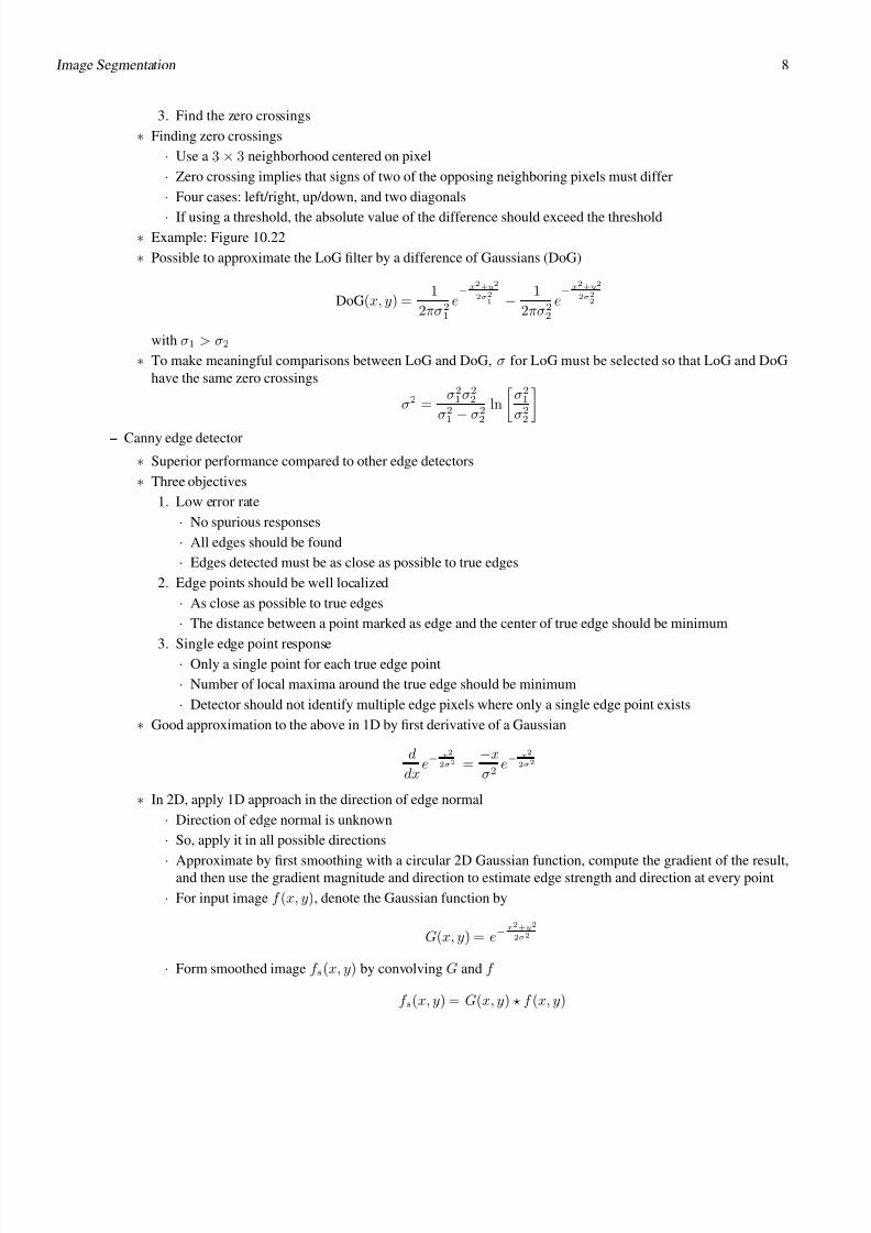
3. Find the zero crossings

∗ Finding zero crossings

· Use a 3 × 3 neighborhood centered on pixel

· Zero crossing implies that signs of two of the opposing neighboring pixels must differ

· Four cases: left/right, up/down, and two diagonals

· If using a threshold, the absolute value of the difference should exceed the threshold∗ Example: Figure 10.22

∗ Possible to approximate the LoG filter by a difference of Gaussians (DoG)

DoG(x, y) =1

2πσ21

e−x2+y2

2σ21 − 1

2πσ22

e−x2+y2

2σ22

with σ1 > σ2

∗ To make meaningful comparisons between LoG and DoG, σ for LoG must be selected so that LoG and DoG

have the same zero crossings

σ2 =σ21

σ22

σ21

−σ22

ln

σ21

σ22

– Canny edge detector

∗ Superior performance compared to other edge detectors

∗ Three objectives

1. Low error rate

· No spurious responses

· All edges should be found

· Edges detected must be as close as possible to true edges

2. Edge points should be well localized

· As close as possible to true edges

· The distance between a point marked as edge and the center of true edge should be minimum

3. Single edge point response· Only a single point for each true edge point

· Number of local maxima around the true edge should be minimum

· Detector should not identify multiple edge pixels where only a single edge point exists

∗ Good approximation to the above in 1D by first derivative of a Gaussian

d

dxe−

x2

2σ2 =−x

σ2e−

x2

2σ2

∗ In 2D, apply 1D approach in the direction of edge normal

· Direction of edge normal is unknown

· So, apply it in all possible directions

· Approximate by first smoothing with a circular 2D Gaussian function, compute the gradient of the result,and then use the gradient magnitude and direction to estimate edge strength and direction at every point

· For input image f (x, y), denote the Gaussian function by

G(x, y) = e−x2+y2

2σ2

· Form smoothed image f s(x, y) by convolving G and f

f s(x, y) = G(x, y) f (x, y)




· Compute the gradient magnitude and direction

M (x, y) =

g2x + g2y

α(x, y) = tan−1

gygx

where gx = ∂f s/∂x and gy = ∂f s/∂y

· M (x, y) typically contains wide ridges around local maxima

· Thin those ridges using nonmaxima suppression

· Specify a number of discrete orientations of the edge normal (gradient vector)

· In a 3 × 3 region, define four orientations as horizontal, vertical, and ±45◦ (Figure 10.24a)

· Define a range of directions over which an edge is considered to be horizontal (Figure 10.24b)

· Figure 10.24c: Angle ranges corresponding to four directions under consideration

· Denote four basic directions by: d1 = horizontal, d2 = −45◦, d3 = vertical, and d4 = +45◦

· Formulate the nonmaxima suppression scheme for a 3 × 3 region centered at every point (x, y) in α(x, y)

1. Find the direction dk that is closest to α(x, y)

2. If the value of M (x, y) is less than at least one of its two neighbors long dk, let gN (x, y) = 0 (suppres-sion); otherwise, let gN (x, y) = M (x, y)

· Threshold gN (x, y) to reduce false edge points

· With single thresholding

1. Threshold too low implies false positives

2. Threshold too high eliminates valid edge points (false negatives)

· Hysteresis thresholding using two thresholds – low threshold T L and high threshold T H ; T H : T L should

be 3 : 1 or 2 : 1

· Thresholding creates two additional images

gNH (x, y) = gN (x, y) ≥ T H

gNL (x, y) = gN (x, y) ≥ T L

· All the nonzero pixels in gNH are contained in gNL

· Eliminate all the nonzero pixels contained in gNH from gNL

gNL(x, y)− = gNH (x, y)

· Now, the nonzero pixels in gNH (x, y) and gNL(x, y) are considered strong and weak edge pixels

· All strong pixels are marked as valid pixels

· Edges in gNH (x, y) may have gaps that are filled by

1. Locate the next unvisited pixel p in gNH (x, y)

2. Mark as valid edge pixels all the weak pixels in gNL(x, y) that are connected to p using 8-connectivity

3. If all nonzero pixels in gNH (x, y) have been visited, go to step 4, otherwise go to step 14. Set to zero all pixels in gNL(x, y) that did not get marked as valid edge pixels

· Form the output by adding gNH (x, y) and gNL (x, y)

∗ Summary of Canny edge detector

1. Smooth the input image by a Gaussian filter

2. Compute the gradient magnitude and angle images

3. Apply nonmaxima suppression to gradient magnitude image

4. Use double thresholding and connectivity analysis to detect and link edges

∗ Typically, follow the detector by an edge-thinning algorithm

∗ Figure 10.25




∗ Example 10.9: Figure 10.26

– Quality vs speed comparisons

• Edge linking and boundary detection

– Pixels may not characterize edges completely because of noise, breaks in edges due to nonuniform illumination,

and other spurious discontinuities in intensity values– Follow edge detection by linking algorithms to assemble edge pixels into meaningful edges or region boundaries

– Local processing

Thresholding

• Central to image segmentation

• Foundation

– Partition images directly into regions based on intensity values and/or properties of these values

– Basics of intensity thresholding

∗ Figure 10.35a: Intensity histogram

∗ Light objects on a dark background

∗ Intensity values grouped into two distinct modes

∗ Select a threshold T that separates these modes

∗ The segmented image g(x, y) is given by

g(x, y) =

1 if f (x, y) > T 0 if f (x, y) ≤ T

where the points labeled 1 are called object points and other points are called background points

∗If T is constant in the above expression, the thresholding is called global thresholding

∗ When the value of T changes over an image, the thresholding is called variable thresholding

∗ Local or regional thresholding

· Variable thresholding in which the value of T at any point depends on its neighborhood

· If T depends on the location itself, the thresholding is called dynamic or adaptive thresholding

∗ Figure 10.35b

· Histogram with three dominant modes

· Possibly two types of light objects on a dark background

· Use multiple thresholding to classify some points to the background and other points to two separate

objects

g(x, y) = a if f (x, y) > T 2b if T 1 < f (x, y)

≤T 2

c if f (x, y) ≤ T 1

∗ Success of thresholding is directly related to the width and depth of valleys separating the histogram modes

∗ Key factors affecting the valley properties

1. Separation between peaks

2. Noise content of the image

3. Relative sizes of objects and background

4. Uniformity of illumination source

5. Uniformity of reflectance properties of the image

– Role of noise in image thresholding




∗ Figure 10.36

– Role of illumination and reflectance

∗ Figure 10.37

– Noise and illumination may not be easily controllable

• Basic global thresholding

– Automatic estimation of global threshold value

1. Select an initial estimate for global threshold T

2. Segment the image using T ,giving G1 as group of object pixels and G2 as group of background pixels

3. Compute average intensity m1 and m2 corresponding to G1 and G2, respectively

4. Compute a new threshold value

T =1

2(m1 + m2)

5. Repeat steps 2 to 4 until the difference between values of T in successive iterations is smaller than a predefined

parameter ∆T

– Works well when there is a reasonabley clear valley between the modes of the histogram corresponding to objects

and background

– ∆T is used to control the number of iterations

– Initial threshold value should be somewhere between the minimum and maximum intensity values in the image

∗ Average intensity of the image is a good initial value

– Figure 10.38

• Variable thresholding

– Variable thresholding based on local image properties

∗ Based on specific properties computed in a neighborhood

∗Mean mxy and standard deviation σxy of pixels in the neighborhood S xy of every point (x, y) in the image

· Descriptors of average intensity and local contrast

∗ Common forms of variable, local thresholds

T xy = aσxy + bmxy

T xy = aσxy + bmG

where a and b are nonnegative constants and mG is the global image mean

∗ Segmented image is computed as

g(x, y) =

1 if f (x, y) > T xy0 if f (x, y) ≤ T xy

∗ Can also use a predicate based on parameters in the pixel neighborhood

g(x, y) =

1 if Q(local parameters) is true

0 if Q(local parameters) is false

∗ Consider the following predicate Q(σxy, mxy) based on local mean and standard deviation

Q(σxy, mxy) =

true if f (x, y) > aσxy&&f (x, y) > bmxy

false otherwise

∗ Figure 10.48

Documents

Segment Good