segDeepM: Exploiting Segmentation and Context in Deep Neural Networks forObject Detection

Yukun Zhu Raquel Urtasun Ruslan Salakhutdinov Sanja FidlerUniversity of Toronto

{yukun,urtasun,rsalakhu,fidler}@cs.toronto.edu

Abstract

In this paper, we propose an approach that exploits ob-ject segmentation in order to improve the accuracy of objectdetection. We frame the problem as inference in a MarkovRandom Field, in which each detection hypothesis scoresobject appearance as well as contextual information usingConvolutional Neural Networks, and allows the hypothesisto choose and score a segment out of a large pool of ac-curate object segmentation proposals. This enables the de-tector to incorporate additional evidence when it is avail-able and thus results in more accurate detections. Our ex-periments show an improvement of 4.1% in mAP over theR-CNN baseline on PASCAL VOC 2010, and 3.4% over thecurrent state-of-the-art, demonstrating the power of our ap-proach.

1. Introduction

In the past two years, Convolutional Neural Networks(CNNs) have revolutionized computer vision. They havebeen applied to a variety of general vision problems, suchas recognition [15, 9], segmentation [11], stereo [18],flow [24], and even text-from-image generation [13], con-sistently outperforming past work. This is mainly due totheir high generalization power achieved by learning com-plex, non-linear dependencies across millions of labelledexamples.

It has recently been shown that increasing the depth ofthe network increases the performance by an additional im-pressive margin on the ImageNet challenge [21, 22]. It re-mains to be seen whether recognition can be solved by sim-ply pushing the limits of computation (the size of the net-works) and increasing the amount of the training data. Webelieve that the main challenge in the next few years will beto design computationally simpler and more efficient mod-els that can achieve a similar or better performance com-pared to the very deep networks.

For object detection, a successful approach has been to

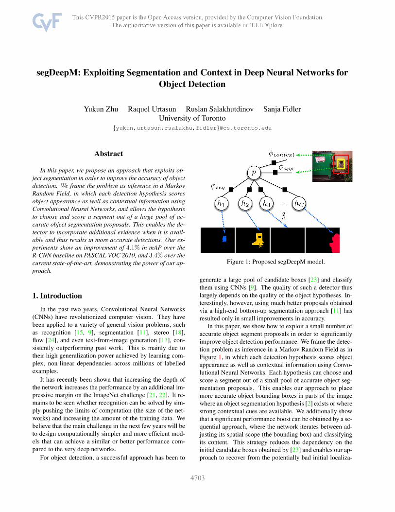
Figure 1: Proposed segDeepM model.

generate a large pool of candidate boxes [23] and classifythem using CNNs [9]. The quality of such a detector thuslargely depends on the quality of the object hypotheses. In-terestingly, however, using much better proposals obtainedvia a high-end bottom-up segmentation approach [11] hasresulted only in small improvements in accuracy.

In this paper, we show how to exploit a small number ofaccurate object segment proposals in order to significantlyimprove object detection performance. We frame the detec-tion problem as inference in a Markov Random Field as inFigure 1, in which each detection hypothesis scores objectappearance as well as contextual information using Convo-lutional Neural Networks. Each hypothesis can choose andscore a segment out of a small pool of accurate object seg-mentation proposals. This enables our approach to placemore accurate object bounding boxes in parts of the imagewhere an object segmentation hypothesis [2] exists or wherestrong contextual cues are available. We additionally showthat a significant performance boost can be obtained by a se-quential approach, where the network iterates between ad-justing its spatial scope (the bounding box) and classifyingits content. This strategy reduces the dependency on theinitial candidate boxes obtained by [23] and enables our ap-proach to recover from the potentially bad initial localiza-

1

tion.We show that our model, called segDeepM, outperforms

the baseline R-CNN [9] approach by 3.2% with almost noextra computational cost. We get a total of 5% improvementby incorporating contextual information at the cost of dou-bling the running time of the method. On PASCAL VOC2010 test, our method achieves 4.1% improvement over R-CNN and 1.4% over the current state-of-the-art.

2. Related WorkIn the past years, a variety of segmentation algorithms

that exploit object detections as a top-down cue have beenexplored. The standard approach has been to use detectionfeatures as unary potentials in an MRF [14], or as candidatebounding boxes for holistic MRFs [26, 16]. In [20], seg-mentation within the detection boxes has been performedusing a GrabCut method. In [1], object segmentations arefound by aligning the masks obtained from Poselets [1, 17].

There have been a few approaches to use segmentation toimprove object detection. [10] cast votes for the object’s lo-cation by using a Hough transform with a set of regions. [5]uses DPM to find a rough object location and refines itaccording to color information and occlusion boundaries.In [11], segmentation is used to mask-out the backgroundinside the detection, resulting in improved performance.Segmentation and detection has also been addressed in ajoint formulation in [25] by combining shape informationobtained via DPM parts as well as color and boundary cues.

Our work is inspired by the success of segDPM [8]. Byaugmenting the DPM detector [7] with very simple seg-mentation features that can be computed in constant time,segDPM improved the detection performance by 8% on thechallenging PASCAL VOC dataset. The approach usedsegments computed from the final segmentation output ofCPMC [2] in order to place accurate boxes in parts of theimage where segmentation for the object class of inter-est was available. This idea was subsequently exploitedin [19] by augmenting the DPM with an additional set ofdeformable context “parts” which scored contextual seg-mentation features around the object. In [4], the segDPMdetector [8] was augmented with part visibility reasoning,achieving state-of-the-art results for detection of articulatedclasses. In [6], the authors extended segDPM to incorporatesegmentation compatibility also at the part level.

In this paper, we build on R-CNN framework [9] andtransfer the core ideas of segDPM. We use appearance fea-tures from [15, 9], a rich contextual appearance descriptionaround the object, and a MRF model that is able to exploitsegmentation in a more efficient way than segDPM.

3. Our ApproachThe goal of our approach is to efficiently exploit segmen-

tation and contextual cues in order to facilitate object detec-

tion. Following the R-CNN setup, we compute the SelectiveSearch boxes [23] yielding approximately 2000 object can-didates per image. For each box we extract the last featurelayer of the CNN network [15], that is fine-tuned on thePASCAL dataset as proposed in [9]. We obtain object seg-ment proposals via the CPMC approach [3], although ourapproach is independent of this choice. Following [2], wetake the top 150 proposals given by an object-independentranker, and train class-specific classifiers for all classes ofinterest by the second-order pooling method O2P [2]. Weremove all segments that have less than 1500 pixels. Ourmethod will make use of these segments along with theirclass-specific scores. This is slightly different than segDPMwhich takes only 1 or 2 segments carved out from the finalO2P’s pixel-level labeling of the image.

In the remainder of this section we first define our modeland describe its segmentation and contextual features. Wenext discuss inference and learning. Finally, we detail asequential inference scheme that iterates between correctingthe input bounding boxes and scoring them with our model.

3.1. The segDeepM Model

We define our model as a Markov Random Field withrandom variables that reason about detection boxes, ob-ject segments, and context. Similar to [7, 8], we definep as a random variable denoting the location and scaleof a candidate bounding box in the image. We also de-fine h to be a set of random variables, one for each class,i.e. h = (h1, h2, . . . , hC)

T . Each random variable hc ∈{0, 1, . . . ,H(x)} represents an index into the set of all can-didate segments. Here C is the total number of objectclasses of interest andH(x) is the total number of segmentsin image x. The random variable hc allows each candidatedetection box to choose a segment for each class and scoreits confidence according to the agreement with the segment.The idea is to (1) boost the confidence of boxes that are wellaligned with a high scoring object region proposal for theclass of interest, and (2) adjust its score based on the prox-imity and confidence of region proposals for other classes,serving as context for the model. This is different fromsegDPM that only had a single random variable h whichselected a segment belonging to the detector’s class. It isalso different from [19] in that the model chooses contex-tual segments, and does not score context in a fixed segmen-tation window. Note that hc = 0 indicates that no segmentis selected for class c. This means that either no segmentfor a class of interest is in the vicinity of the detection hy-pothesis, or that none of the regions corresponding to thecontextual class c help classification of the current box. Wedefine the energy of a configuration as follows:

E(p,h;x) = ωTapp · φapp(p;x) + ωT

seg · φseg(p,h;x) (1)

+ ωTctx · φctx(p;x),

where φapp(x, p), φseg(p,h;x), and φctx(p;x) are the can-didate’s appearance, segmentation, and contextual potentialfunctions (features), respectively. We describe the poten-tials in detail below.

3.2. Details of Potential Functions

Appearance: To extract the appearance features we fol-low [9]. The image in each candidate detection’s box iswarped to a fixed size 227 × 227 × 3. We run the im-age through the CNN [15] trained on the ImageNet datasetand fine-tuned on PASCAL’s data [9]. As our appearancefeature φapp(p;x) we use the 4096-dimensional feature ex-tracted from the fc7 layer.

Segmentation: Similar to [8], our segmentation fea-tures attempt to capture the agreement between the candi-date’s bounding box and a particular segment. The featuresare complementary in nature, and, when combined withinthe model, aim at placing the box tightly around each seg-ment. We emphasize that the weights for each feature willbe learned, thus allowing the model to adjust the importanceof each feature’s contribution to the joint energy.

We use slightly more complex features tailored to ex-ploit a much larger set of segments than [8]. In particular,we use a grid feature that aims to capture a loose geometricarrangement of the segment inside the candidate’s box. Wealso incorporate class information, where the model is al-lowed to choose a different segment for each class, depend-ing on the contextual information contained in a segmentwith respect to the class of the detector.

We use multiple segmentation features, one for eachclass, thus our segmentation term decomposes:

ωTseg · φseg(p,h;x) =

∑c∈{1,...,C}

∑type

ωTtype · φtype(p, hc;x).

Specifically, we consider the following features:SegmentGrid-In: Let S(hc) denote the binary mask of

the segment chosen by hc. For a particular candidate box p,we crop the segment’s mask via the bounding box of p andcompute the SegmentGrid-in feature on a K × K grid Gplaced over the cropped mask. The kth dimension rep-resents the percentage of segment’s pixels inside the kth

block, relative to the number of all pixels in S(hc).

φseggrid−in(x, p, hc, k) =1

|S(hc)|∑

i∈G(p,k)

S(hc, i), (2)

where G(p, k) is the kth block of pixels in grid G, andS(hc, i) indexes the segment’s mask in pixel i. That is,S(hc, i) = 1 when pixel i is part of the segment andS(hc, i) = 0 otherwise. For c matching the detector’sclass, this feature will attempt to place a box slightly biggerthan the segment while at the same time trying to localize itsuch that the spatial distribution of pixels within each grid

matches the class’ expected shape. For c other than the de-tector’s class, this feature will try to place the box such thatit intersects as little as possible with the segments of otherclasses. The dimensionality of this feature is K ×K × C.

Segment-Out: This feature follows [8], and computesthe percentage of segment pixels outside the candidate box.Unlike the SegmentGrid-In, this feature computes a singlevalue for each segment/bounding box pair.

φseg−out(p, h) =1

|S(h)|∑

i 6∈B(p)

S(h, i), (3)

where B(p) is the bounding box corresponding to p. Theaim of this feature is to place boxes that are smallercompared to the segments, which, in combination withSegmentGrid-In, achieves a tight fit around the segments.

BackgroundGrid-In: This feature is also computedwith a K×K grid G for each bounding box p. We computethe percentage of pixels in each grid cell that are not part ofthe segment:

φback−in(p, h, k) =1

M − |S(h)|∑

i∈G(p,k)

(1− S(h, i)) ,

(4)with M the area of the largest segment for the image.

Background-Out: This scalar feature measures the %of segment’s background outside of the candidate’s box:

φback−out(p, h) =1

M − |S(h)|∑

i6∈B(p)

(1− S(h, i)) . (5)

Overlap: Similarly to [8], we use another feature tomeasure the alignment of the candidate’s box and the seg-ment S(h). It is computed as the intersection-over-union(IOU) between the box or p and a tightly fit bounding boxaround the segment S(h).

φoverlap(x, p, h) =B(p) ∩ B(S(x, h))B(p) ∪ B(S(x, h))

− λ, (6)

where B(S(x, h)) is tight box around S(x, h), and λ a biasterm which we set to λ = −0.7 in our experiments.

SegmentClass: Since we are dealing with many seg-ments per image, we add an additional feature to our model.We train the O2P [2] rankers for each class which uses sev-eral region-aware features as input into our segmentationfeatures. Each ranker is trained to predict the IOU over-lap of the given segment with the ground-truth object’s seg-ment. The output of all the class-specific rankers defines thefollowing feature:

φpotential(h, c) =1

1 + e−s(h,c), (7)

where s(h, c) is the score of class c for segment S(h).

SegmentGrid-in, segment-out, backgroundGrid-in, andbackground-out can be efficiently computed via integral im-ages [8]. Note that [8]’s features are a special case of thesefeatures with a grid size K = 1. Overlap and segment fea-tures can also be quickly computed using matrix operations.

Context: CNNs are typically trained for the task of im-age classification where in most cases an input image ismuch larger than the object. This means that part of theirsuccess may be due to learning complex dependencies be-tween the objects and their contextual information (e.g. skyfor aeroplane, road for car and bus). However, the appear-ance features that we use are only computed based on thecandidate’s box, thus hardly capturing useful informationfrom the scene. We thus add an additional feature that looksat a bigger scope than the candidate’s box.

In particular, we enlarge each input candidate box by afixed percentage ρ along its horizontal and vertical direc-tion. For big boxes, or those close to the image boundary,we clip the enlarged region to be fully inside the image. Wekeep the object labels for each expanded box the same asthat for the original boxes, even if the expanded box nowencloses objects of other classes. We then warp the imagein each enlarged box to 227×227 and fine-tune the originalImageNet-trained CNN using these images and labels. Wecall the fine-tuned network the expanded CNN. For our con-textual features φctx(x, p) we extract the fc7 layer featuresof the expanded CNN by running the warped image in theenlarged window through the network.

3.3. Inference

In the inference stage of our model, we score each can-didate box p as follows:

fw(x, p) = maxh

(ωTapp · φapp(x, p) + ωT

ctx · φctx(x, p)

+ ωTseg · φseg(x, p,h)

). (8)

Observe that the first two terms in Eq. 8 can be computedefficiently by matrix multiplication, and the only part thatdepends on h is its last term. Although there could be expo-nential number of candidates for h, we can greedily searcheach dimension of h and find the best segment S(hc) w.r.t.model parameters ωseg for each class c. Since our segmen-tation features do not depend on the pairwise relationshipsin h, this greedy approach is guaranteed to find the globalmaximum of ωT

seg · φseg(x, p,h). Finally, we sum the threeterms to obtain the score of each bounding box location p.

3.4. Learning

Given a set of images with N candidate boxes {pn} andtheir annotations {y(xn, pn)}, together with a collection ofsegments for each image {S(xn, hn)} and associated po-tentials {φ(xn, hn)} with n = 1, .., N , training our model

can be written as follows:

minω‖ω‖2 + C

N∑n=1

max (0, 1− y(xn, pn)fw(xn, pn)) ,

(9)where ω is a vector of all the weights in our model.

The learning problem in (9) is a latent SVM [7] wherewe treat the assignment variable h as a latent variable foreach training instance. To optimize Equation (9), we iteratetwo steps following [7]:

1. label each positive example: for each (x, p) withy(x, p) = 1, we compute h∗ = argmaxh fw(x, p)with current the model parameters ω;

2. update the weights: we do hard-negative mining over aset of negative instances until reaching a certain mem-ory limit. We then use stochastic gradient descent tooptimize the weights ω.

Latent SVM is guaranteed to converge to a local min-imum only, thus we need to carefully pick a good initial-ization for positive examples at the first iteration. We usethe overlap feature φoverlap as the indicator and set eachdimension of h∗ as h∗ = argmaxh φoverlap(p,h). Thisencourages the method to pick segments that best overlapswith the candidate’s box.

Although our segmentation features are efficient to com-pute, we need to recompute them for all positive examplesduring the first step and for all hard negative examples dur-ing the second step of training. In our implementation, wecache a pool of segmentation features φseg(x, p,h) for alltraining instances to avoid computing them in every itera-tion. With the compact segmentation feature, our methodachieves similar running speed with that of R-CNN [9].

3.5. Iterative Bounding Box Prediction

As a typical postprocessing step, object detection ap-proaches usually perform bounding box prediction on theirfinal candidate set [7, 9]. This typically results in a few per-cent improvement in accuracy, since the approach is able tomake an informative re-localization based on complex fea-tures. Following [9], we also use pool5 layer features inorder to do bounding box prediction.

In this paper we take this idea one step further by doingbounding box prediction and scoring the model in an itera-tive fashion. Our motivation is that better localization canlead to improved predictions. In particular, we first extractthe CNN features and regress to a corrected set of boxes. Wethen re-extract the features on the new boxes and score ourmodel. We only re-extract the features on the boxes whichhave changed by more than 20% percent from the originalset. We can then repeat this process, by doing bounding boxprediction again, re-extracting the features, and re-scoring.

seg exp ibr br plane bike bird boat bottle bus car cat chair cow table dog horse motor person plant sheep sofa train tv mAP

RCNN 69.9 64.2 48.0 30.2 26.9 63.3 56.0 67.6 26.8 44.7 29.6 61.7 55.7 69.8 56.4 26.6 56.7 35.6 54.4 57.7 50.1RCNN+CPMC 71.5 65.3 48.6 31.5 27.9 64.3 57.2 67.6 26.7 46.2 33.6 62.8 57.8 70.7 57.9 26.6 54.0 37.8 57.0 57.6 51.1segDPM+CNN

√72.8 64.1 50.7 32.1 28.2 64.9 55.9 72.4 27.7 50.6 31.7 65.9 59.3 71.1 57.1 26.5 59.4 38.8 57.1 57.6 52.2

segDeepM√

73.8 64.0 52.4 32.7 28.2 66.4 56.7 73.1 28.1 51.4 34.0 66.1 59.9 71.0 56.6 29.5 59.5 43.9 61.6 58.0 53.3segDeepM

√72.2 65.2 52.4 36.3 29.4 67.3 59.0 71.0 28.9 49.1 30.6 67.6 59.3 72.6 59.1 28.7 60.6 38.6 58.2 60.3 53.3

segDeepM√

71.4 64.3 50.2 31.8 30.6 66.0 57.5 68.7 25.6 49.7 30.5 64.7 58.3 69.9 60.7 26.9 54.4 35.0 57.1 55.5 51.4segDeepM

√ √74.5 64.8 55.3 36.3 31.2 69.0 59.0 73.8 29.7 53.3 33.7 68.8 62.3 73.1 59.3 29.8 63.1 41.3 63.4 60.0 55.1

segDeepM√ √ √

77.1 67.4 58.2 36.9 37.4 71.3 61.1 74.4 29.3 56.3 34.8 69.8 64.1 72.7 64.1 31.5 60.0 39.7 64.8 58.2 56.4RCNN

√72.9 65.8 54.0 34.5 31.2 68.0 59.8 72.3 26.6 51.3 35.0 65.7 59.7 71.7 60.7 28.0 60.6 37.1 60.3 59.9 53.7

segDeepM√ √

76.9 66.8 57.8 36.2 32.2 71.4 60.0 75.4 27.7 53.8 38.6 68.6 64.4 72.6 61.1 30.4 61.5 43.2 64.1 60.9 56.2segDeepM

√ √76.7 68.7 58.0 39.9 34.6 71.1 62.1 75.9 30.3 54.6 36.2 69.6 63.3 74.0 63.5 31.3 62.5 37.9 66.3 61.0 56.9

segDeepM√ √

77.2 66.6 55.2 34.5 34.6 67.5 60.0 70.4 27.1 53.4 35.9 66.4 63.4 71.9 63.0 32.0 55.7 38.5 62.0 58.0 54.7segDeepM

√ √ √77.2 67.6 59.8 40.2 35.7 72.0 62.1 75.7 30.4 58.1 37.2 69.9 64.8 73.9 63.4 32.4 63.9 43.1 68.4 61.6 57.9

segDeepM√ √ √ √

79.0 70.6 61.9 40.4 39.0 71.6 61.9 74.7 31.3 56.6 39.2 70.4 66.5 73.5 65.6 35.3 60.7 44.3 68.0 58.7 58.5

Table 1: Detection results (in % AP) on PASCAL VOC 2010 val for R-CNN and segDeepM detectors..

seg exp ibr br plane bike bird boat bottle bus car cat chair cow table dog horse motor personplant sheep sofa train tv mAP

RCNN 74.4 69.0 55.6 34.5 35.2 70.8 63.0 81.4 35.0 57.9 39.3 77.7 70.2 75.8 61.7 29.1 66.9 56.7 63.8 58.7 58.8segDeepM

√77.5 67.7 59.0 33.4 35.9 71.3 62.4 82.8 35.6 61.4 42.7 79.1 70.7 76.7 62.3 31.3 67.1 54.0 65.5 60.0 59.8

segDeepM√

77.4 72.9 62.6 36.8 39.4 71.5 64.9 83.7 37.1 62.0 40.4 81.0 73.1 77.9 65.7 34.7 68.0 59.1 70.0 58.7 61.8segDeepM

√ √79.2 69.8 63.6 36.4 39.5 72.9 65.2 83.5 38.4 63.6 43.8 80.8 75.1 78.3 66.2 33.3 68.6 56.0 70.7 60.2 62.2

RCNN√

78.6 72.1 62.1 40.4 40.0 71.2 65.0 84.2 36.7 59.5 41.8 80.3 74.5 78.0 65.8 33.0 67.3 59.9 68.7 61.3 62.0segDeepM

√ √79.0 71.3 63.0 38.9 40.0 72.8 63.4 84.9 36.7 62.1 44.3 80.2 76.0 78.7 66.0 35.8 68.3 57.8 67.5 62.0 62.4

segDeepM√ √

81.6 74.6 66.6 41.6 44.6 70.7 68.0 84.9 39.7 62.5 44.2 84.1 77.1 79.2 69.9 35.7 67.6 60.9 72.7 61.3 64.4segDeepM

√ √ √81.5 73.4 66.6 40.4 44.7 71.3 67.5 85.1 40.9 62.9 46.0 83.5 76.9 80.0 70.0 37.1 68.9 60.4 72.2 61.1 64.5

Table 2: Detection results (in % AP) on PASCAL VOC 2010 val for RCNN and segDeepM using 16 layer OxfordNet CNN..

plane bike bird boat bottle bus car cat chair cow table dog horse motor person plant sheep sofa train tv mAP

segDeepM-16 layers 82.3 75.2 67.1 50.7 49.8 71.1 69.5 88.2 42.5 71.2 50.0 85.7 76.6 81.8 69.3 41.5 71.9 62.2 73.2 64.6 67.2segDeepM-8 layers 75.3 69.7 57.6 44.2 42.1 62.2 64.7 74.8 30.1 55.6 43.1 70.7 66.4 72.6 63.5 31.9 61.9 46.1 64.4 58.1 57.8BabyLearning 77.7 73.8 62.3 48.8 45.4 67.3 67.0 80.3 41.3 70.8 49.7 79.5 74.7 78.6 64.5 36.0 69.9 55.7 70.4 61.7 63.8R-CNN (breg)-16 ly. 79.3 72.4 63.1 44.0 44.4 64.6 66.3 84.9 38.8 67.3 48.4 82.3 75.0 76.7 65.7 35.8 66.2 54.8 69.1 58.8 62.9R-CNN-16 layers 76.5 70.4 58.0 40.2 39.6 61.8 63.7 81.0 36.2 64.5 45.7 80.5 71.9 74.3 60.6 31.5 64.7 52.5 64.6 57.2 59.8Feature Edit 74.8 69.2 55.7 41.9 36.1 64.7 62.3 69.5 31.3 53.3 43.7 69.9 64.0 71.8 60.5 32.7 63.0 44.1 63.6 56.6 56.4R-CNN (breg) 71.8 65.8 53.0 36.8 35.9 59.7 60.0 69.9 27.9 50.6 41.4 70.0 62.0 69.0 58.1 29.5 59.4 39.3 61.2 52.4 53.7R-CNN 67.1 64.1 46.7 32.0 30.5 56.4 57.2 65.9 27.0 47.3 40.9 66.6 57.8 65.9 53.6 26.7 56.5 38.1 52.8 50.2 50.2

Table 3: State-of-the-art detection results (in %AP) on PASCAL VOC 2010 test. The 16 layer models adopt OxforNet, therest use 8-layer AlexNet..

seg exp ibr br plane bike bird boat bottle bus car cat chair cow table dog horse motor personplant sheep sofa train tv mAP

RCNN 68.9 63.5 45.6 29.1 26.7 64.4 55.6 69.5 26.3 50.3 36.1 62.2 55.6 68.7 56.0 27.6 54.8 40.2 54.0 60.5 50.8segDeepM

√ √ √75.1 67.6 56.6 37.9 34.6 73.8 60.8 76.1 27.6 55.4 39.1 68.9 63.7 72.4 63.8 33.5 60.8 45.9 65.7 60.9 57.0

RCNN√

74.0 66.7 50.4 32.9 31.5 68.0 58.4 74.7 26.9 52.9 39.3 67.0 59.2 71.5 59.1 29.9 56.8 44.2 63.1 63.7 54.5segDeepM

√ √ √ √77.3 70.2 60.2 39.8 38.3 75.2 62.3 76.1 29.4 55.7 40.8 70.5 66.4 72.4 65.8 35.6 60.9 46.1 66.7 63.5 58.7

Table 4: Detection results (in % AP) on PASCAL VOC 2012 val for RCNN and segDeepM detectors..

Our experiments show that this procedure converges to a setof stable boxes after two iterations.

4. Experimental EvaluationWe evaluate our method on the main object detection

benchmark PASCAL VOC. We provide a details ablativestudy of different potentials and choices in our model inSubsec. 4.1. In Subsec. 4.2 we test our method on PAS-CAL’s held-out test set and compare it to the current state-of-the-art methods.

4.1. A Detailed Analysis of Our Model on Val

We first evaluate our detection performance on V al setof the PASCAL VOC 2010 detection dataset. We train allmethods on the train subset and evaluate the detection per-formance using the standard PASCAL criterion. We provide

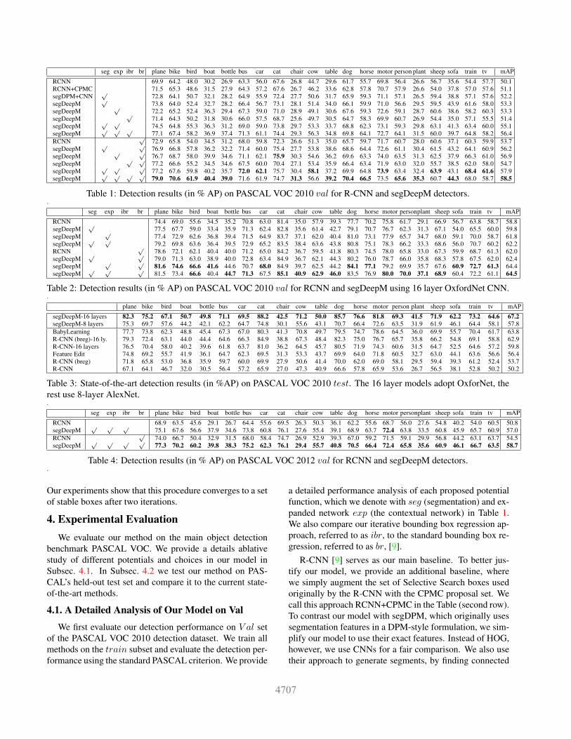
a detailed performance analysis of each proposed potentialfunction, which we denote with seg (segmentation) and ex-panded network exp (the contextual network) in Table 1.We also compare our iterative bounding box regression ap-proach, referred to as ibr, to the standard bounding box re-gression, referred to as br, [9].

R-CNN [9] serves as our main baseline. To better jus-tify our model, we provide an additional baseline, wherewe simply augment the set of Selective Search boxes usedoriginally by the R-CNN with the CPMC proposal set. Wecall this approach RCNN+CPMC in the Table (second row).To contrast our model with segDPM, which originally usessegmentation features in a DPM-style formulation, we sim-plify our model to use their exact features. Instead of HOG,however, we use CNNs for a fair comparison. We also usetheir approach to generate segments, by finding connected

recall0 0.2 0.4 0.6 0.8 1

pre

cis

ion

0

0.2

0.4

0.6

0.8

1 class: aeroplane, subset: val

RCNN, AP=69.9RCNN(br), AP=72.9segDeepM, AP=77.1segDeepM(br), AP=79.0

(a) PR curve for plane

recall0 0.2 0.4 0.6 0.8 1

pre

cis

ion

0

0.2

0.4

0.6

0.8

1 class: bicycle, subset: val

RCNN, AP=64.2RCNN(br), AP=65.8segDeepM, AP=67.4segDeepM(br), AP=70.6

(b) PR curve for bicycle

recall0 0.2 0.4 0.6 0.8

pre

cis

ion

0

0.2

0.4

0.6

0.8

1 class: bird, subset: val

RCNN, AP=48.0RCNN(br), AP=54.0segDeepM, AP=58.1segDeepM(br), AP=61.9

(c) PR curve for bird

recall0 0.2 0.4 0.6 0.8

pre

cis

ion

0

0.2

0.4

0.6

0.8

1 class: boat, subset: val

RCNN, AP=30.2RCNN(br), AP=34.5segDeepM, AP=36.9segDeepM(br), AP=40.3

(d) PR curve for boat

recall0 0.2 0.4 0.6 0.8

pre

cis

ion

0

0.2

0.4

0.6

0.8

1 class: bottle, subset: val

RCNN, AP=26.9RCNN(br), AP=31.2segDeepM, AP=37.4segDeepM(br), AP=39.0

(e) PR curve for bottle

recall0 0.2 0.4 0.6 0.8 1

pre

cis

ion

0

0.2

0.4

0.6

0.8

1 class: bus, subset: val

RCNN, AP=63.3RCNN(br), AP=68.0segDeepM, AP=71.3segDeepM(br), AP=71.6

(f) PR curve for bus

recall0 0.2 0.4 0.6 0.8

pre

cis

ion

0

0.2

0.4

0.6

0.8

1 class: car, subset: val

RCNN, AP=56.0RCNN(br), AP=59.8segDeepM, AP=61.1segDeepM(br), AP=61.9

(g) PR curve for car

recall0 0.2 0.4 0.6 0.8 1

pre

cis

ion

0

0.2

0.4

0.6

0.8

1 class: cat, subset: val

RCNN, AP=67.6RCNN(br), AP=72.3segDeepM, AP=74.4segDeepM(br), AP=74.7

(h) PR curve for cat

recall0 0.2 0.4 0.6 0.8

pre

cis

ion

0

0.2

0.4

0.6

0.8

1 class: chair, subset: val

RCNN, AP=26.8RCNN(br), AP=26.6segDeepM, AP=29.2segDeepM(br), AP=31.3

(i) PR curve for chair

recall0 0.2 0.4 0.6 0.8

pre

cis

ion

0

0.2

0.4

0.6

0.8

1 class: cow, subset: val

RCNN, AP=44.7RCNN(br), AP=51.3segDeepM, AP=56.3segDeepM(br), AP=56.5

(j) PR curve for cow

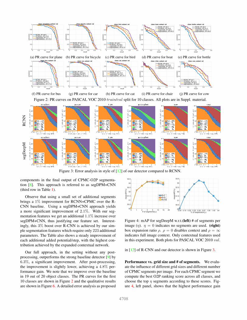
Figure 2: PR curves on PASCAL VOC 2010 train/val split for 10 classes. All plots are in Suppl. material.

RC

NN

segD

eepM

Figure 3: Error analysis in style of [12] of our detector compared to RCNN.

components in the final output of CPMC-O2P segmenta-tion [8]. This approach is referred to as segDPM+CNN(third row in Table 1).

Observe that using a small set of additional segmentsbrings a 1% improvement for RCNN+CPMC over the R-CNN baseline. Using a segDPM+CNN approach yieldsa more significant improvement of 2.1%. With our seg-mentation features we get an additional 1.1% increase oversegDPM+CNN, thus justifying our feature set. Interest-ingly, this 3% boost over R-CNN is achieved by our sim-ple segmentation features which require only 223 additionalparameters. The Table also shows a steady improvement ofeach additional added potential/step, with the highest con-tribution achieved by the expanded contextual network.

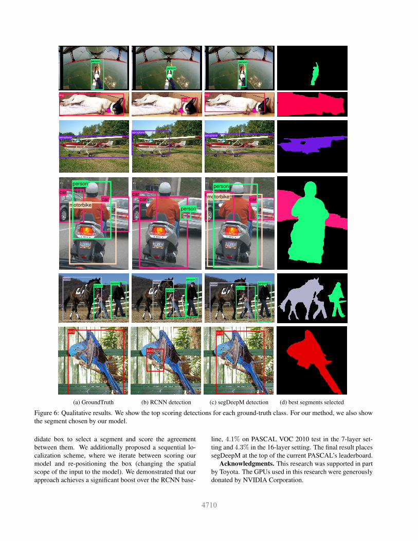
Our full approach, in the setting without any post-processing, outperforms the strong baseline detector [9] by6.3%, a significant improvement. After post-processing,the improvement is slightly lower, achieving a 4.8% per-formance gain. We note that we improve over the baselinein 19 out of 20 object classes. The PR curves for the first10 classes are shown in Figure 2 and the qualitative resultsare shown in Figure 6. A detailed error analysis as proposed

# of segments(η)0 1 2 3 5 10 15 20

mea

nAP(

%)

50

50.5

51

51.5

52

52.5

53

53.5

K=1K=3K=10

% of expansion(ρ)0.00 0.10 0.20 0.33 0.50 0.67 1.00 1.43 Inf

mea

nAP(

%)

50

50.5

51

51.5

52

52.5

53

53.5

Figure 4: mAP for segDeepM w.r.t.(left) # of segments perimage (η). η = 0 indicates no segments are used. (right)box expansion ratio ρ. ρ = 0 disables context and ρ = ∞indicates full image context. Only contextual features usedin this experiment. Both plots for PASCAL VOC 2010 val.

in [12] of R-CNN and our detector is shown in Figure 3.

Performance vs. grid size and # of segments. We evalu-ate the influence of different grid sizes and different numberof CPMC segments per image. For each CPMC segment wecompute the best O2P ranking score across all classes, andchoose the top η segments according to these scores. Fig-ure 4, left panel, shows that the highest performance gain

is due to the few best scoring segments. The differencesare minor across different values of K and η. Interestingly,the model performs worse with more segments and a coarsegrid, as additional low-quality segments add noise and makeL-SVM training more difficult. When using a finer grid,the performance peaks when more segments are use, andachieves an overall improvement over a single-cell grid.

Performance w.r.t. expansion ratio. We evaluate the in-fluence of the box expansion ratio ρ used in our contextualmodel. The results for varying values of ρ are illustrated inFigure 4, right panel. Note that even a small expansion ratio(10% in each direction) can boost the detection performanceby a significant 1.5%, and the performance reaches its peakat ρ = 0.5. This indicates that richer contextual informa-tion leads to a better object recognition. Notice also that thedetection performance decreases beyond ρ = 0.5. This ismost likely due to the fact that most contextual boxes ob-tained this way will cover most or even the full image, andthus the positive and negative training instances in the sameimage will share the identical contextual features. This con-fuses our classifier and results in a performance loss. If wetake the full image as context, the gain is less than 1%.

Iterative bounding box prediction. We next study theeffect of iterative bounding box prediction. We report a1.4% gain over the original R-CNN by starting with ourset of re-localized boxes (one iteration). Note that re-localization in the first iteration only affects 52% of boxes(only 52% of boxes change more than 20% from the orig-inal set, thus feature re-computation only affects half ofthe boxes). This performance gain persists when combinedwith our full model. If we apply another bounding boxprediction as a post-processing step, this approach still ob-tains a 0.6% improvement over R-CNN with bounding boxprediction. In this iteration, re-localization affects 42% ofboxes. We have noticed that the performance saturates aftertwo iterations. The second iteration improves mAP by onlya small margin (about 0.1%). The interesting side result isthat, the mean Average Best Overlap (mABO) measure usedby bottom-up proposal generation techniques [23] to bench-mark their proposals, remains exactly the same (85.6%)with or without our bounding box prediction, but has a sig-nificant impact on the detection performance. This may in-dicate that mABO is not the best or at least not the onlyindicator of a good bottom-up grouping technique.

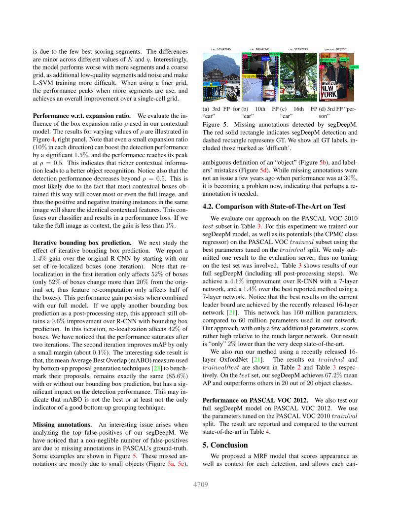
Missing annotations. An interesting issue arises whenanalyzing the top false-positives of our segDeepM. Wehave noticed that a non-neglible number of false-positivesare due to missing annotations in PASCAL’s ground-truth.Some examples are shown in Figure 5. These missed an-notations are mostly due to small objects (Figure 5a, 5c),

chairchairdiningtablechairchair

car: 165/47245.

(a) 3rd FP for“car”

diningtable

person personpersoncar

bottle

car: 266/47245.

(b) 10th FP“car”

bicycle

car: 312/47245.

(c) 16th FP“car”

personpersonperson

persondog

person: 86/32061.

(d) 3rd FP “per-son”

Figure 5: Missing annotations detected by segDeepM.The red solid rectangle indicates segDeepM detection anddashed rectangle represents GT. We show all GT labels, in-cluded those marked as ’difficult’.

ambiguous definition of an “object” (Figure 5b), and label-ers’ mistakes (Figure 5d). While missing annotations werenot an issue a few years ago when performance was at 30%,it is becoming a problem now, indicating that perhaps a re-annotation is needed.

4.2. Comparison with State-of-The-Art on Test

We evaluate our approach on the PASCAL VOC 2010test subset in Table 3. For this experiment we trained oursegDeepM model, as well as its potentials (the CPMC classregressor) on the PASCAL VOC trainval subset using thebest parameters tuned on the train/val split. We only sub-mitted one result to the evaluation server, thus no tuningon the test set was involved. Table 3 shows results of ourfull segDeepM (including all post-processing steps). Weachieve a 4.1% improvement over R-CNN with a 7-layernetwork, and a 1.4% over the best reported method using a7-layer network. Notice that the best results on the currentleader board are achieved by the recently released 16-layernetwork [21]. This network has 160 million parameters,compared to 60 million parameters used in our network.Our approach, with only a few additional parameters, scoresrather high relative to the much larger network. Our resultis “only” 2% lower than the very deep state-of-the-art.

We also run our method using a recently released 16-layer OxfordNet [21]. The results on train/val andtrainval/test are shown in Table 2 and Table 3 respec-tively. On the test set, our segDeepM achieves 67.2% meanAP and outperforms others in 20 out of 20 object classes.

Performance on PASCAL VOC 2012. We also test ourfull segDeepM model on PASCAL VOC 2012. We usethe parameters tuned on the PASCAL VOC 2010 train/valsplit. The result are reported and compared to the currentstate-of-the-art in Table 4.

5. ConclusionWe proposed a MRF model that scores appearance as

well as context for each detection, and allows each can-

person

person

person

dog

dog

dog

aeroplane

aeroplaneaeroplane

car

car

motorbike

person

car

car

person

carcarmotorbike

person

horse

personperson

horseperson

person

horse person

person

bird

(a) GroundTruth

bird

(b) RCNN detection

bird

(c) segDeepM detection (d) best segments selected

Figure 6: Qualitative results. We show the top scoring detections for each ground-truth class. For our method, we also showthe segment chosen by our model.

didate box to select a segment and score the agreementbetween them. We additionally proposed a sequential lo-calization scheme, where we iterate between scoring ourmodel and re-positioning the box (changing the spatialscope of the input to the model). We demonstrated that ourapproach achieves a significant boost over the RCNN base-

line, 4.1% on PASCAL VOC 2010 test in the 7-layer set-ting and 4.3% in the 16-layer setting. The final result placessegDeepM at the top of the current PASCAL’s leaderboard.

Acknowledgments. This research was supported in partby Toyota. The GPUs used in this research were generouslydonated by NVIDIA Corporation.

References[1] L. Bourdev, S. Maji, T. Brox, and J. Malik. Detecting peo-

ple using mutually consistent poselet activations. In ECCV,2010. 2

[2] J. Carreira, R. Caseiro, J. Batista, and C. Sminchisescu. Se-mantic segmentation with second-order pooling. In ECCV,pages 430–443. Springer, 2012. 1, 2, 3

[3] J. Carreira and C. Sminchisescu. Constrained parametricmin-cuts for automatic object segmentation. In CVPR, pages3241–3248. IEEE, 2010. 2

[4] X. Chen, R. Mottaghi, X. Liu, N.-G. Cho, S. Fidler, R. Ur-tasun, and A. Yuille. Detect what you can: Detecting andrepresenting objects using holistic models and body parts. InCVPR, 2014. 2

[5] Q. Dai and D. Hoiem. Learning to localize detected objects.In CVPR, 2012. 2

[6] J. Dong, Q. Chen, S. Yan, and A. Yuille. Towards unifiedobject detection and semantic segmentation. In ECCV, pages299–314. Springer, 2014. 2

[7] P. F. Felzenszwalb, R. B. Girshick, D. McAllester, and D. Ra-manan. Object detection with discriminatively trained part-based models. TPAMI, 32(9):1627–1645, 2010. 2, 4

[8] S. Fidler, R. Mottaghi, A. Yuille, and R. Urtasun. Bottom-upsegmentation for top-down detection. In CVPR, 2013. 2, 3,4, 6

[9] R. Girshick, J. Donahue, T. Darrell, and J. Malik. Rich fea-ture hierarchies for accurate object detection and semanticsegmentation. arXiv preprint arXiv:1311.2524, 2013. 1, 2,3, 4, 5, 6

[10] C. Gu, J. Lim, P. Arbelaez, and J. Malik. Recognition usingregions. In CVPR, 2009. 2

[11] B. Hariharan, P. Arbelaez, R. Girshick, and J. Malik. Simul-taneous detection and segmentation. In ECCV, 2014. 1, 2

[12] D. Hoiem, Y. Chodpathumwan, and Q. Dai. Diagnosing errorin object detectors. In ECCV, 2014. 6

[13] R. Kiros, R. Salakhutdinov, and R. Zemel. Multimodal neu-ral language models. In ICML, 2014. 1

[14] P. Krahenbuhl and V. Koltun. Efficient inference in fullyconnected crfs with gaussian edge potentials. In NIPS, 2011.2

[15] A. Krizhevsky, I. Sutskever, and G. E. Hinton. Imagenetclassification with deep convolutional neural networks. InNIPS, pages 1097–1105, 2012. 1, 2, 3

[16] L. Ladicky, P. Sturgess, K. Alahari, C. Russell, and P. H. Torr.What, where and how many? combining object detectors andcrfs. In ECCV, 2010. 2

[17] M. Maire, S. X. Yu, and P. Perona. Object detection andsegmentation from joint embedding of parts and pixels. InICCV, 2011. 2

[18] R. Memisevic and C. Conrad. Stereopsis via deep learning.In NIPS, 2011. 1

[19] R. Mottaghi, X. Chen, X. Liu, N.-G. Cho, S.-W. Lee, S. Fi-dler, R. Urtasun, and A. Yuille. The role of context for ob-ject detection and semantic segmentation in the wild. CVPR,2014. 2

[20] O. Parkhi, A. Vedaldi, C. V. Jawahar, and A. Zisserman. Thetruth about cats and dogs. In ICCV, 2011. 2

[21] K. Simonyan and A. Zisserman. Very deep convolu-tional networks for large-scale image recognition. InarXiv:1409.1556, 2014. 1, 7

[22] C. Szegedy, W. Liu, Y. Jia, P. Sermanet, S. Reed,D. Anguelov, D.Erhan, V. Vanhoucke, and A. Rabi-novich. Going deeper with convolutions. arXiv preprintarXiv:1409.4842, 2014. 1

[23] K. E. Van de Sande, J. R. Uijlings, T. Gevers, and A. W.Smeulders. Segmentation as selective search for objectrecognition. In ICCV, pages 1879–1886. IEEE, 2011. 1,2, 7

[24] P. Weinzaepfel, J. Revaud, Z. Harchaoui, and C. Schmid.DeepFlow: Large displacement optical flow with deepmatching. In ICCV, 2013. 1

[25] Y. Yang, S. Hallman, D. Ramanan, and C. Fowlkes. Layeredobject models for image segmentation. PAMI, 2011. 2

[26] J. Yao, S. Fidler, and R. Urtasun. Describing the scene asa whole: Joint object detection, scene classification and se-mantic segmentation. In CVPR, 2012. 2