0

The Sea Ice Experiment: Dynamic Nature of the Arctic (SEDNA)

Applied Physics Laboratory Ice Station (APLIS) 2007

Field Report Editor: Jennifer K. Hutchings

Sedna by Brenda Jones

1

Table of Contents Participant List 2 1. Introduction 4 2. Remote Sensing Support 18 3. Buoy Deployments 45 4. Ice Thickness Campaign 56 5. Ridge Study 85 6. Perimeter Survey 96 7. Meteorology 106 8. Oceanography 115 9. Outreach 119 Acknowledgements 126 Appendix 1 128 Appendix 2 129 Appendix 3 130 Appendix 4 131 Appendix 5 134 Appendix 6 138 Appendix 7 140 References 143

2

Field Campaign Participants SEDNA Field Participants (incl. remote sensing groups and home support) Rob Chadwell chadwell@iarc.uaf.edu Pablo Clemente-Colon Pablo.clemente-colon@natice.noaa.gov Martin Doble m.j.doble@damtp.cam.ac.uk Bruce Elder bruce.c.elder@erdc.usace.army.mil Rene Forsberg rf@spacecenter.dk Cathy Geiger cgeiger@udel.edu Katharine Giles k.giles@cpom.ucl.ac.uk Scott Grauer-Gray sgrauerg@gmail.com Christian Haas chaas@awi.de Stephan Hendriks Steffan.Hendricks@awi.de Ben Holt ben@pacific.jpl.nasa.gov Nick Hughes nick.hughes@sams.ac.uk Jenny Hutchings jenny@iarc.uaf.edu Chandra Kambhamettu chandrak@UDel.Edu M. McGregor mac.mcgregor@sympatico.ca Eggert Jon Magnusson eggert@gavia.is Torge Martin tmartin@awi-bremerhaven.de Alice Orlich fsaro1@uaf.edu Mitch Osborne Mitch_Osborne@fws.gov Jackie Richter-Menge jacqueline.a.richter-menge@erdc.usace.army.mil Andrew Roberts aroberts@uaf.edu Henriette Skourup hsk@spacecenter.dk Mani Thomas mani@udel.edu Adrian Turner akt@cpom.ucl.ac.uk Peter Wadhams p.wadhams@damtp.cam.ac.uk Jeremy Wilkinson jeremy.wilkinson@sams.ac.uk Richard Yeo richard@gavia.is Jay Zwally zwally@icesat2.gsfc.nasa.gov Other Science Participants Bill Simpson ffwrs@uaf.edu Dan Carlson fsdac8@uaf.edu Matt Pruis matt@nwra.com Skip Echert Media and Education participants Richard Bond Tigress Productions Barney Revill Tigress Productions BarnyRevill@tigressproductions.co.uk Doug Allan Tigress Productions Josh Bernstien Discovery Channel Art Howard PolarPalozza Geoff Haines-Stiles PolarPalozza ghs@passporttoknowledge.com Robert Harris PolarTrec harrisr@hartfordschools.net

3

APLIS Logistics Crew Fred Karig fred@apl.washington.edu Fran Olson Patrick McKeown Kevin Parkhurst Kieth Van Thiel Victoria Simms Stephanie Shawn Lambert

Photo Credit: Art Howard

4

1. Introduction

The mass balance of sea ice, which can be thought of as the evolution of the thickness distribution of the ice cover, is controlled by thermodynamic ice growth and melt, mechanical redistribution through ridging and rafting, and transport. For simplicity, we consider a regional Lagrangian frame of reference, and track the evolution of a region of ice, eliminating the need to consider transport. Thermodynamic forcing is typically modeled as uniform across a region or smoothly varying with latitude, snow cover and cloud cover. The impact of forcing on the growth or melt rate of level ice is dominated by heterogeneity at the meter scale, associated with spatial variability of ice thickness, snow depth and surface conditions [Perovich et al., 2003]. The heterogeneity of sea ice is controlled by the super-position of the thermodynamic response (growth/melt) on an icescape created by mechanical redistribution (leads, ridging, and rafting). Relatively speaking, thermodynamically-driven change over a highly variable (meter scale) ice cover occurs gradually with thermodynamic processes controlled by the annual solar radiation cycle. On the other hand, mechanical redistribution of the ice cover occurs abruptly and predominantly in the winter with linear regions of deformation manifested in leads and ridges. Leads are kilometers long, 10s to 100s of meters wide, and are often aligned into systems of leads. Analysis of RADARSAT SAR imagery [Kwok, 2001], shows that lead systems often extend 100s of kilometers across the Arctic Basin, and these "linear kinematic features" (LKFs) display strain rates an order of magnitude higher than the surrounding ice pack. Ice growth in leads results in level ice, which is often ridged or rafted when these leads close. Ridges and rafts introduce meter-scale heterogeneity into the spatial distribution of ice thickness. These processes constantly rework the surface morphology on sub-daily and synoptic time scales. Thus, sea ice deformation serves as the initial sculptor of spatial variability of sea ice thickness and surface morphology. It is the process of ice deformation and its impact on the mass balance of the sea ice cover that is the focus of this project. Global Climate Models (GCM) projections of future ice extent show ice receding, and loss of the perennial ice zone, though models disagree on the rate of recession [ACIA, 2005]. Models used in the ACIA study all have very different constitutive models, thermodynamic models and atmospheric dynamics. As the sensitivity of ice thickness to thermodynamic parameterizations, dynamic parameterizations, and ocean/wind forcing variability are comparable (see for example [Steele and Flato, 1999; Kreyscher et al., 2000]), it is not possible to isolate the cause of the difference between these models. One way to improve these models is to identify the magnitude and direction of feedbacks on the ice mass balance, and build accurate parameterizations of ocean-ice-atmosphere coupling described by these feedbacks. We do not know whether dynamic effects result in negative or positive feedback

5

to sea ice mass decrease in a warming climate. For example, in a weakening ice pack, we could expect divergence to increase as resistance to closure decreases. Hence the ice ridging rate could increase (a negative feedback). On the other hand, large scale changes in ice drift and increased surface wave activity from an associated increase in fetch length might result in less compression against the coast and multi-year ice zone, hence reducing the ridging yet increasing new ice growth (potentially a positive feedback). To determine the sign and magnitude of this feedback we must improve our understanding of how new ice growth, ridging and rafting will respond to such things as: (a) increasing storminess in the Arctic; (b) a seasonal ice pack of reduced thickness; and (c) large scale changes in drift modifying ice stress. 1.1 Objectives Central Hypothesis High frequency spatial and temporal variability of sea ice mass balance is primarily driven by pack ice-ocean dynamical response to changes in wind forcing. Questions we address to determine the temporal and spatial distribution of lead and ridging events and establish appropriate constitutive and mechanical redistribution models are:

• Do popular parameterizations of ridging, rafting and open water fraction, coupled with popular constitutive models for pack ice, reproduce observed thickness distribution?

• Is deformation coherent in time across 10 - 100km spatial scales, with a power law scaling?

The first goal of our proposed project is to improve our understanding of the relationship between sea ice thickness variability and sea ice motion variability by investigating stress and strain-rate relations with a comprehensive suite of spatiotemporal coincident observations. We wish to characterize how sea ice deformation controls the spatial variability of pack ice from the kilometer scale up. Our second goal is to determine if the viscous-plastic sea ice model, in a configuration used in current and next generation climate models, can realistically simulate the impact of ice dynamics on sea ice mass balance. An additional goal is to determine optimal sets of measurements with which to monitor pan-Arctic sea ice mass balance, utilizing model sensitivity studies to determine model uncertainties and identify key monitoring needs To accomplish these goals, we focus on the following objectives.

1. Characterize the relationship between strain rate and changes in the regional thickness distribution.

2. Characterize the relationship between, and coherence of, stress and strain rate at 10km and 100km.

3. Test theoretical relationships between stress, strain rate, and regional

6

thickness distribution. 4. Validate models of ice dynamics: How well do they reproduce observed

sea ice mass balance given known strain rates or realistic wind stress fields?

We address these objectives with a joint field-remote sensing-modeling campaign, taking advantage of the location and season of the U.S. Navy Ice Camp in spring 2007. Our campaign built upon previous individual efforts, by coordinating modeling, remote sensing and field expertise to provide an integrated view of the spatiotemporal variability of sea ice deformation and its impact on the sea ice mass balance. By synchronizing an ice thickness measurement campaign with deformation measurements, we will be able to perform a detailed analysis of the inter-relation between sea ice stress, strain and mass balance. 1.2 Justification This project brings the above research threads in sea ice field work, remote sensing and modelling, to provide a holistic view of sea ice failure and thickness redistribution on geophysical scales. A comprehensive set of sea ice measurements will be taken to develop and validate models of both thermodynamic and dynamic processes for sea ice, across all the scales that dynamic and thermodynamic processes vary. This enables us to design and assess optimal measurement methods for Arctic-wide monitoring of sea ice mass balance utilizing models, remote sensing and in situ measurements. 1.2.1 Basis for the campaign

Table 1.1: The scales and methods of measurement for variables in Eqn. 1, with link to the

section where measurement campaign is discussed.

Variable Point 1km 10km 100km Regional Sec. Growth/

Melt f IMB buoy Forsberg,E

M-bird, submarine

Forsberg,EM-bird Model 3.3, 4.2.3, 4.2.2

Surface stress

FO

FA Wind tower, ADCP

NCAR/NCEP, ECMWF,NARR

reanalysis

NCAR/NCEP, ECMWF,NARR

reanalysis

7,8

Internal ice stress

σ stress sensor

Stress Senor Array

Stress Senor Array

Stress Senor Array

3.2

Strain rate ε& SAR GPS, SAR GPS, SAR SAR, IABP 2.1, 3.1

Ridge parameters

φ On foot, diving

transects

UAV/Forsberg

Forsberg Forsberg Model 5, 6

Thickness distribution

g Drill holes Calibration transects

EM-bird, Forsberg, submarine

EM-bird, Forsberg ICEsat, Model 4, 2.5

7

To meet our goals, we have designed a field campaign that will provide information about all phenomena that control the sea ice mass balance (Table 1). These measurements must allow separation of thermodynamic and dynamic effects on the ice thickness distribution, and determine the relative effect of dynamic processes on new ice growth, ridging and rafting. Let us take a look at the equations governing sea ice mass balance. Consider a region of ice of area A described by a thickness distribution function )(hg , such that ∫ = 1gdh and the ice mass in the region is ∫= Aghdhm . Following this region of ice in a Lagrangian frame of reference, the thickness distribution will evolve according to φ+

∂∂

=∂∂

hfg

tg , (1)

where is the thermodynamic rate of change of thickness (ice growth or melt) and is the mechanical redistribution function (leads, ridging and rafting). The growth or melt rate is determined from the energy balance over the ice sheet, given by EFLSFF wswlw =++++ , (2) where is the energy available for melt or growth of ice. The other terms are downwelling longwave flux absorbed (Flw), downwelling shortwave flux absorbed (Fsw), sensible heat flux (S), latent heat flux (L), and heat flux from the ocean to ice respectively (Fw). We can estimate for a region of ice by (a) measuring the rate of change of ice thickness for all thicknesses of level and ridged ice in the region; or by (b) measuring the individual terms in the energy balance to estimate, and determining how much ice grows or melts. The second option is complicated by the facts that: the ice/snow surface is heterogeneous in space and time, resulting in non-uniform absorption of shortwave and longwave radiation; and leads strongly influence the magnitude of S, L and Fw. As the focus of this project is to understand the effect of dynamics on the mass balance we opt to characterize f with the first option (see Sec. 3.3). The redistribution function is directly related to the divergence of ice in the region. There are a variety of models for redistribution of sea ice thickness, and they typically have the form fraction opening opening mode + fraction ridging/rafting closing mode).

(εφ &= fraction opening ∗ opening mode + fraction ridging/rafting ∗ closing mode). (3)

First consider the strain rate, ε& , a tensor with components of velocity gradients, which is related to the internal stress of the ice pack. We can measure strain rate with SAR-derived products (see Sec. 2.1) and buoy drift (see Sec. 3.1). The strain rate is modeled by considering the momentum balance on the ice given by

,σ⋅∇++++= GCAO FFFFdt

dmu (4)

where σ⋅∇ is the divergence of the internal ice stress. This stress is related to

8

strain by a constitutive relation for the material. Relationships between sea ice stress and strain rate are viscous-plastic [Hibler, 1979], elasto-plastic [Pritchard, 1976] or Mohr-Coulomb [Trembley and Mysak, 1997]. There is debate over what scales particular constitutive relations and plastic yield criteria apply [Overland et al., 1995; Schulson and Hibler, 2004] It is thought that the constitutive model for sea ice might be scale invariant, though this is not proven for geophysical scales. Marsden et al. [2004] show strain rate follows a power law spatial scaling relation. SEDNA includes a campaign to investigate the relationship between sea ice stress and strain rate using SAR (Sec. 2.1), GPS buoys( Sec 3.1), and stress gauges (Sec 3.2). The other components in the momentum balance are ocean stress ( OF ), wind stress ( AF ), Coriolis force ( CF ) and gravitational potential down the sea surface slope ( GF ). Of these, OF and AF are the same magnitude as σ⋅∇ . Not surprisingly then, the sensitivities of model ice thickness to variability of surface stresses and variations in constitutive relation are of comparable magnitude [Hutchings, 2001]. To simulate the sea ice stress, strain rate and lead behavior, we need surface forcing fields that accurately represent direction, spatial gradient and position of winds and currents (see Sec. 7 and Sec. 8). Our measurements will provide validation of model forcing fields and an estimation of the stress loading on the ice pack. Next, we consider the other components in the redistribution function, namely the parameterization of the ridging and rafting behavior. In large scale mechanical redistribution models: (1) ridges are parameterized with a simple shape (triangular [Hibler, 1980], level [Rothrock, 1975]); (2) mechanical redistribution is assumed to be volume conserving (i.e., ridges contain no voids); (3) ridging occurs under shear (an exception being the Roberts [2005] scheme designed for high resolution continuum models); and (4) it is often assumed a fixed fraction of open water always exists in the "closed mode". These models have been developed with concepts derived from statistical analysis of a wide variety of thickness data. Our proposed campaign will observe all variables required to investigate the physical process of ridge building, relating deformation to mechanical redistribution. To validate ridging models we require information about: how ice blocks are incorporated into ridges and ridge porosity; the mean ridge shape and thickness variability; and open water fraction. To validate large scale mechanical redistribution models, we require information about the evolution of the thickness distribution on 10-100km scales. A measurement campaign to characterize ridge shape and density is presented in Sec. 5. These measurements will be used in analysis of aerial laser profiling of freeboard combined with underwater ice draft surveys, to determine volume of ridges created during specific redistribution events. The thin ice end of the ice

9

thickness distribution will be measured (Sec. 4), to relate the area of open leads to strain rate. All measurements will be used in direct validation of strain constrained mechanical redistribution models. To close the system of measurements, we need to monitor the evolution of the sea ice thickness distribution in the region. We present a thickness monitoring campaign over connected scales,1km - regional (see Table 1), in Sec. 4. 1.3 Overview of the field campaign The Applied Physics Laboratory Ice Station (APLIS) was set up in February 2007, and run for Naval operations during March 2007. APLIS was handed over to the National Science Foundation (NSF) for scientific field work on April 1st. NSF funded scientists occupied the camp until April 15th, and the camp was disbanded on April 16th. The camp was initially located 190 miles north of Prudhoe Bay, and was serviced by Cessna Caravan flights during April. A Bell 212 helicopter was present between April 1st and March 13th. The helicopter was used for all remote buoy deployments and to collect ice thickness data with EM-bird. We also used the helicopter to provide three aerial surveys of the ice camp and transport to the remote location where the HMS HMS Tireless recorded multi-beam sonar data. On March 13th the helicopter flew to Barrow, recording EM-bird data along track. The ice camp was also visited by the Canadian Ice Service Dash-8 reconnaissance aircraft on April 2nd, and by a Danish National Space Center Twin Otter on April 12th. Three snow machines where available for transportation to field sites around the camp. There was a heavy need for the machines, so their use was carefully managed and shared between groups. The majority of the SEDNA in-situ survey work was done on foot. Snow machines where only used for transportation to the Ridge Survey site (sec. 5), and to perform Perimeter surveys (sec. 6). In the previous section we describe measurements required to resolve redistribution-stress-strain rate processes on scales of 1km, 10km, 100km and Regional. To tie our measurements together into a campaign that provides the necessary information at each scale (see Table 1.1), required considerable coordination between research groups. This coordination was provided by developing the structure of the field campaign around nested buoy arrays. Two hexagonal buoy arrays defined the 10km and 100km scales. The measurement campaign followed a wheel and spoke design, to resolve ice thickness distribution along lines that radiated out from the camp to GPS drifting buoy and between buoys. The 1km scale was in rigid motion, and its thickness distribution was resolved in a set of calibration lines that mirrored the hexagonal structure of the two buoy arrays.

10

Over the calibration transects (sec 4.1) and at one ridge study site (sec. 5), all ice thickness measurement methods available at the camp were inter-compared. The AWI EM-bird was flown along 10km transects, and Rene Forsberg provided laser altimetry data over roughly half the area of the 10km array. Peter Wadhams performed sonar surveys from the HMS Tireless within the 10km array. Unfortunately, due to difficulty in communication with the classified camp, the submarine tracks do not align exactly with the 10km buoy array. We included an extra 1km calibration line to provide direct validation of submarine sonar ice draft data. The transects of the 70km array were flown by EM-bird. One line of this array was surveyed by Rene Forsberg’s laser altimeter. It was not possible, during the Navy time allotted, to survey ice draft by submarine over the 70km array. We augmented strain rate and meteorological measurements on the regional scale by deploying 3 IABP buoys 100 miles from the ice camp in the North, East and West directions. Spatial coverage of sea ice deformation will be extended across the Beaufort Sea region through analysis of RADARSat ScanSAR-B imagery (see sec. 2.1). IceSat and EnviSat Altimetry provided pan-Arctic coverage of sea ice thickness throughout the field campaign. Unfortunatly, during the short two week period of the camp, there were no IceSat or EnviSat orbits falling close enough to the camp to allow direct validation of the satellite ice thickness products. Additional surveys with EM-bird, submarine and the Danish Twin Otter provided ice thickness information on long (>100mile) transects in the Beaufort Sea.

11

Figure 1.1: Buoy positions over plotted on a RADARSat ScanSAR-B scene, showing the location of the ice camp in the Beaufort Sea (buoy array center) on April 5th. (Red diamonds: meteorological beacons; green diamonds: GPS drifters; yellow dots: stress sensors; blue dot: ice mass balance buoy; pink dots: GPS drifters clusted along individual leads). Red lines show discontinuities in ice motion field, calculated between two SAR images on April 5th and 8th.

12

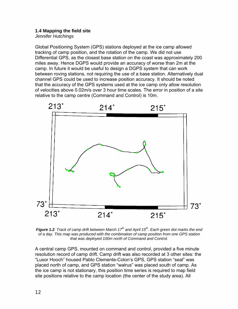
1.4 Mapping the field site Jennifer Hutchings Global Positioning System (GPS) stations deployed at the ice camp allowed tracking of camp position, and the rotation of the camp. We did not use Differential GPS, as the closest base station on the coast was approximately 200 miles away. Hence DGPS would provide an accuracy of worse than 2m at the camp. In future it would be useful to design a DGPS system that can work between roving stations, not requiring the use of a base station. Alternatively dual channel GPS could be used to increase position accuracy. It should be noted that the accuracy of the GPS systems used at the ice camp only allow resolution of velocities above 0.02m/s over 3 hour time scales. The error in position of a site relative to the camp centre (Command and Control) is 10m.

Figure 1.2: Track of camp drift between March 17th and April 15th. Each green dot marks the end

of a day. This map was produced with the combination of camp position from one GPS station that was deployed 100m north of Command and Control.

A central camp GPS, mounted on command and control, provided a five minute resolution record of camp drift. Camp drift was also recorded at 3 other sites: the “Luxor Hooch” housed Pablo Clemente-Colon’s GPS, GPS station “seal” was placed north of camp, and GPS station “walrus” was placed south of camp. As the ice camp is not stationary, this position time series is required to map field site positions relative to the camp location (the center of the study area). All

13

position measurements were recorded with a time stamp, at minute resolution. Hence we are able to build a map of survey sites around the camp, for sites that were in rigid motion with the camp. The map in figure 1.3 was produced using walrus as the reference station. Locations were translated so that Command and Control falls at the center of the camp coordinate system. Note that the camp was rotating, so the camp coordinate system would rotate in geographical space over time.

Figure 1.3: Map of continuous ice around the APLIS 2007 camp. The active ridge/cracks shown

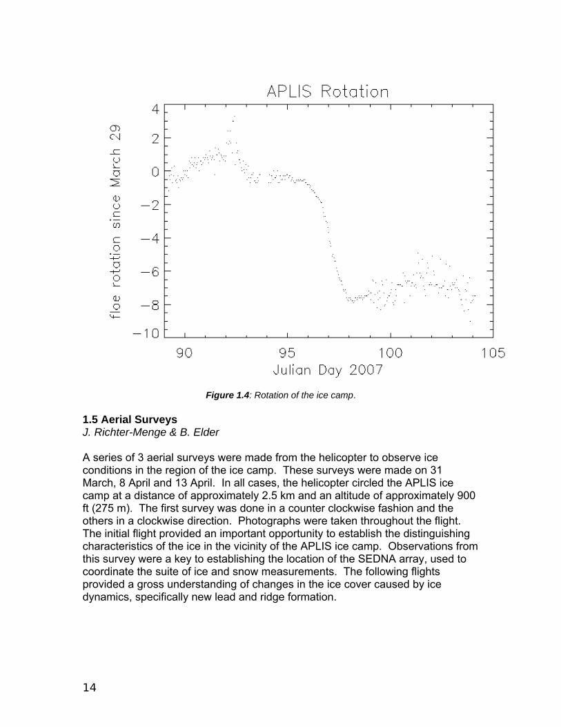
on the map defined the perimeter of our in-situ survey area. In order to map the position of the ice floe in relation to surrounding ice, it is important to know the rotation of the ice floe. To calculate rotation to better than 2o resolution, requires that 2 GPS receivers be placed at least 100m apart. We placed two receivers 200m North (seal) and 200m South (walrus) of the camp. Floe rotation was calculated for the seal to walrus, walrus to command&control, and seal to command&control baselines. The ice floe rotation is shown in figure 1.3. Note the 8o rotation event that occurred on April 6th and 7th. This corresponded to shear ridging in roughly the North-South direction, close to the camp to both the East and West. At this point in time the ice camp was surrounded by active ridges on all sides, which probably allowed for this unusual rotation event.

14

Figure 1.4: Rotation of the ice camp.

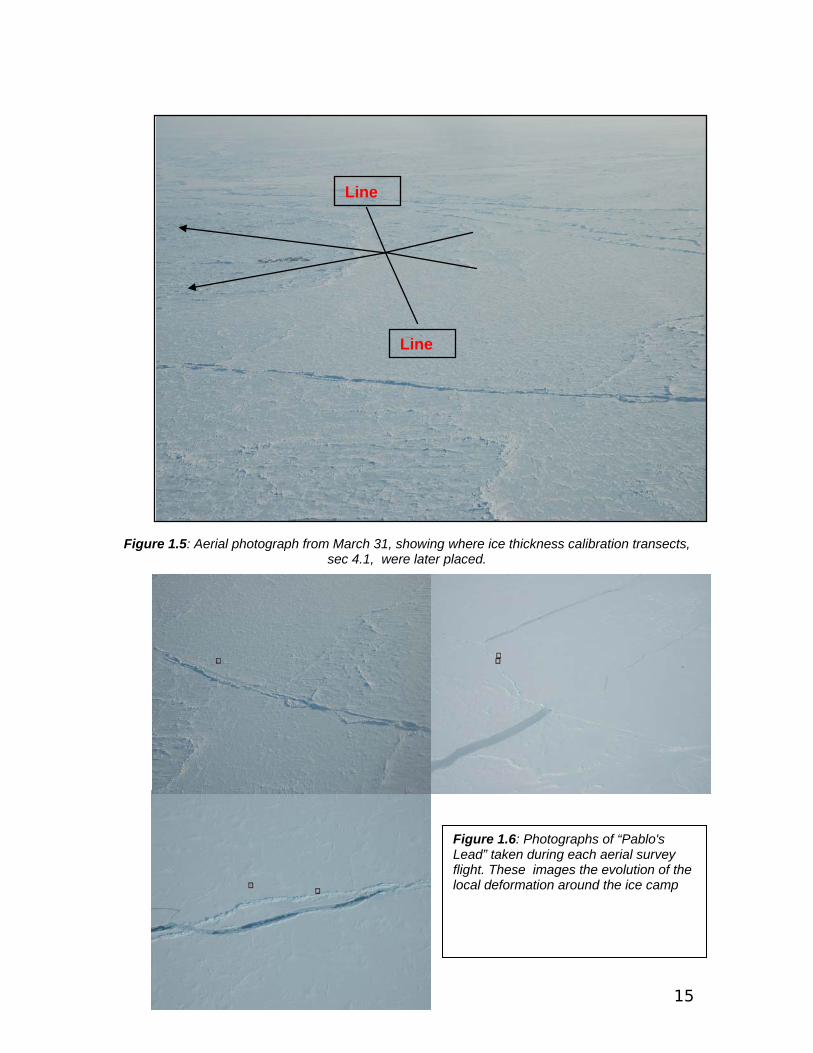
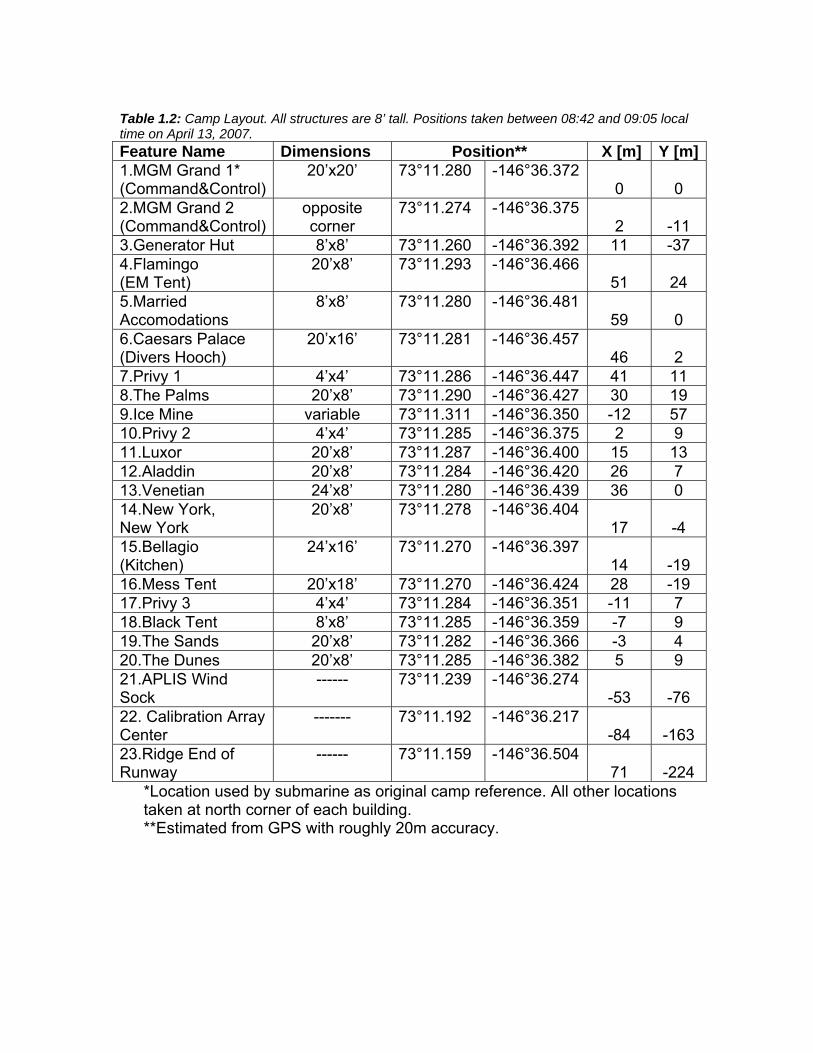
1.5 Aerial Surveys J. Richter-Menge & B. Elder A series of 3 aerial surveys were made from the helicopter to observe ice conditions in the region of the ice camp. These surveys were made on 31 March, 8 April and 13 April. In all cases, the helicopter circled the APLIS ice camp at a distance of approximately 2.5 km and an altitude of approximately 900 ft (275 m). The first survey was done in a counter clockwise fashion and the others in a clockwise direction. Photographs were taken throughout the flight. The initial flight provided an important opportunity to establish the distinguishing characteristics of the ice in the vicinity of the APLIS ice camp. Observations from this survey were a key to establishing the location of the SEDNA array, used to coordinate the suite of ice and snow measurements. The following flights provided a gross understanding of changes in the ice cover caused by ice dynamics, specifically new lead and ridge formation.

15

Figure 1.5: Aerial photograph from March 31, showing where ice thickness calibration transects,

sec 4.1, were later placed.

Figure ??:.

Line

Line

Figure 1.6: Photographs of “Pablo's Lead” taken during each aerial survey flight. These images the evolution of the local deformation around the ice camp

16

1.6 Camp Layout Cathleen Geiger

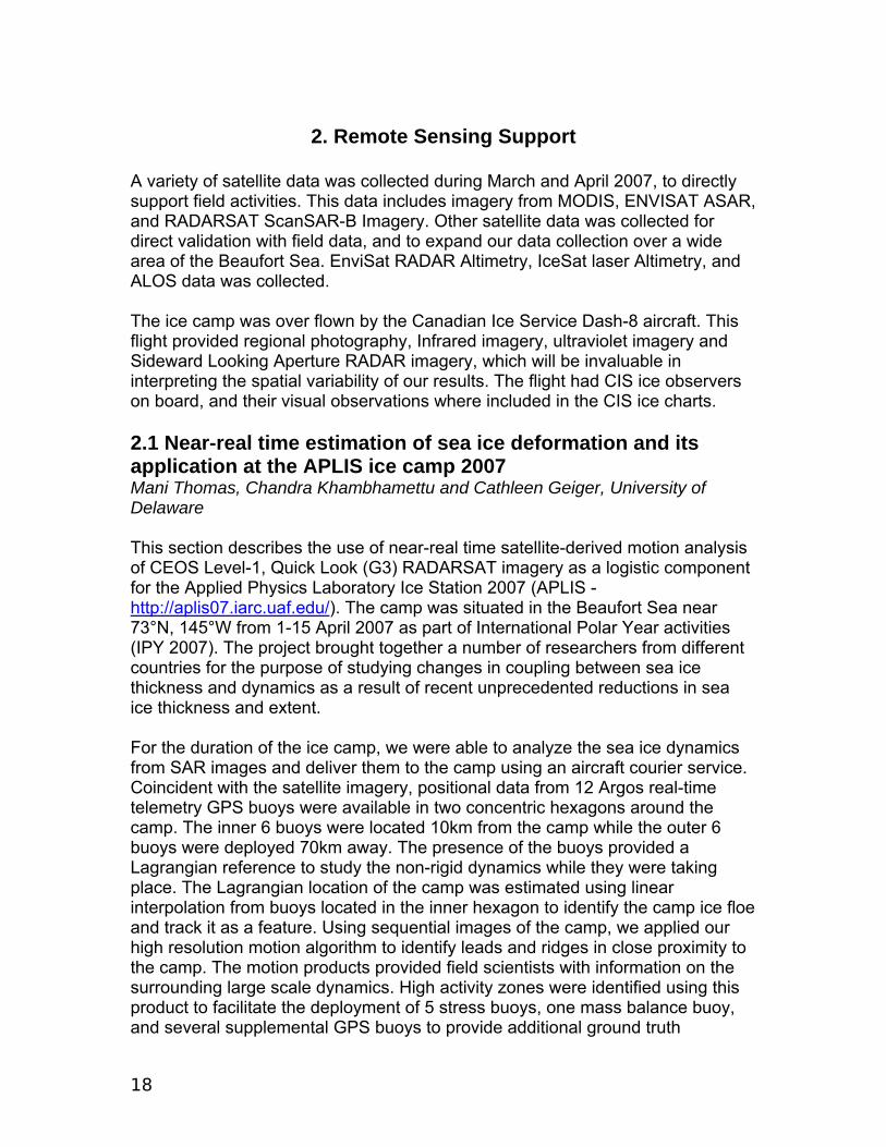
A handheld GPS survey was made of the ice camp, mapping the location of each building. Figure 1.7 shows the map created. The labels on figure 1.7 are expanded in table 1.2. Sample Preliminary Results Show example pictures left and right view of one detailed shot pair (frost flowers) and larger view pair (big ridge). Summary Summarize based on the figures to be added in results section

1

2

3

4

5

6

17

10

7CampPole

8

9

11

12

13

14

15

16

1918

20 1

2

1

2

3

4

5

6

1717

1010

77CampPole

8

99

11

12

13

14

15

16

15

16

191818

20

Figure 1.7: Overview of camp layout

17

Table 1.2: Camp Layout. All structures are 8’ tall. Positions taken between 08:42 and 09:05 local time on April 13, 2007. Feature Name Dimensions Position** X [m] Y [m]1.MGM Grand 1* (Command&Control)

20’x20’ 73°11.280 -146°36.372 0 0

2.MGM Grand 2 (Command&Control)

opposite corner

73°11.274 -146°36.375 2 -11

3.Generator Hut 8’x8’ 73°11.260 -146°36.392 11 -37 4.Flamingo (EM Tent)

20’x8’ 73°11.293 -146°36.466 51 24

5.Married Accomodations

8’x8’ 73°11.280 -146°36.481 59 0

6.Caesars Palace (Divers Hooch)

20’x16’ 73°11.281 -146°36.457 46 2

7.Privy 1 4’x4’ 73°11.286 -146°36.447 41 11 8.The Palms 20’x8’ 73°11.290 -146°36.427 30 19 9.Ice Mine variable 73°11.311 -146°36.350 -12 57 10.Privy 2 4’x4’ 73°11.285 -146°36.375 2 9 11.Luxor 20’x8’ 73°11.287 -146°36.400 15 13 12.Aladdin 20’x8’ 73°11.284 -146°36.420 26 7 13.Venetian 24’x8’ 73°11.280 -146°36.439 36 0 14.New York, New York

20’x8’ 73°11.278 -146°36.404 17 -4

15.Bellagio (Kitchen)

24’x16’ 73°11.270 -146°36.397 14 -19

16.Mess Tent 20’x18’ 73°11.270 -146°36.424 28 -19 17.Privy 3 4’x4’ 73°11.284 -146°36.351 -11 7 18.Black Tent 8’x8’ 73°11.285 -146°36.359 -7 9 19.The Sands 20’x8’ 73°11.282 -146°36.366 -3 4 20.The Dunes 20’x8’ 73°11.285 -146°36.382 5 9 21.APLIS Wind Sock

------ 73°11.239 -146°36.274 -53 -76

22. Calibration Array Center

------- 73°11.192 -146°36.217 -84 -163

23.Ridge End of Runway

------ 73°11.159 -146°36.504 71 -224

*Location used by submarine as original camp reference. All other locations taken at north corner of each building. **Estimated from GPS with roughly 20m accuracy.

18

2. Remote Sensing Support

A variety of satellite data was collected during March and April 2007, to directly support field activities. This data includes imagery from MODIS, ENVISAT ASAR, and RADARSAT ScanSAR-B Imagery. Other satellite data was collected for direct validation with field data, and to expand our data collection over a wide area of the Beaufort Sea. EnviSat RADAR Altimetry, IceSat laser Altimetry, and ALOS data was collected. The ice camp was over flown by the Canadian Ice Service Dash-8 aircraft. This flight provided regional photography, Infrared imagery, ultraviolet imagery and Sideward Looking Aperture RADAR imagery, which will be invaluable in interpreting the spatial variability of our results. The flight had CIS ice observers on board, and their visual observations where included in the CIS ice charts. 2.1 Near-real time estimation of sea ice deformation and its application at the APLIS ice camp 2007 Mani Thomas, Chandra Khambhamettu and Cathleen Geiger, University of Delaware This section describes the use of near-real time satellite-derived motion analysis of CEOS Level-1, Quick Look (G3) RADARSAT imagery as a logistic component for the Applied Physics Laboratory Ice Station 2007 (APLIS - http://aplis07.iarc.uaf.edu/). The camp was situated in the Beaufort Sea near 73°N, 145°W from 1-15 April 2007 as part of International Polar Year activities (IPY 2007). The project brought together a number of researchers from different countries for the purpose of studying changes in coupling between sea ice thickness and dynamics as a result of recent unprecedented reductions in sea ice thickness and extent. For the duration of the ice camp, we were able to analyze the sea ice dynamics from SAR images and deliver them to the camp using an aircraft courier service. Coincident with the satellite imagery, positional data from 12 Argos real-time telemetry GPS buoys were available in two concentric hexagons around the camp. The inner 6 buoys were located 10km from the camp while the outer 6 buoys were deployed 70km away. The presence of the buoys provided a Lagrangian reference to study the non-rigid dynamics while they were taking place. The Lagrangian location of the camp was estimated using linear interpolation from buoys located in the inner hexagon to identify the camp ice floe and track it as a feature. Using sequential images of the camp, we applied our high resolution motion algorithm to identify leads and ridges in close proximity to the camp. The motion products provided field scientists with information on the surrounding large scale dynamics. High activity zones were identified using this product to facilitate the deployment of 5 stress buoys, one mass balance buoy, and several supplemental GPS buoys to provide additional ground truth

19

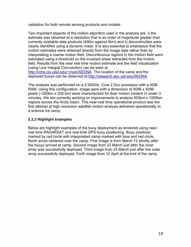
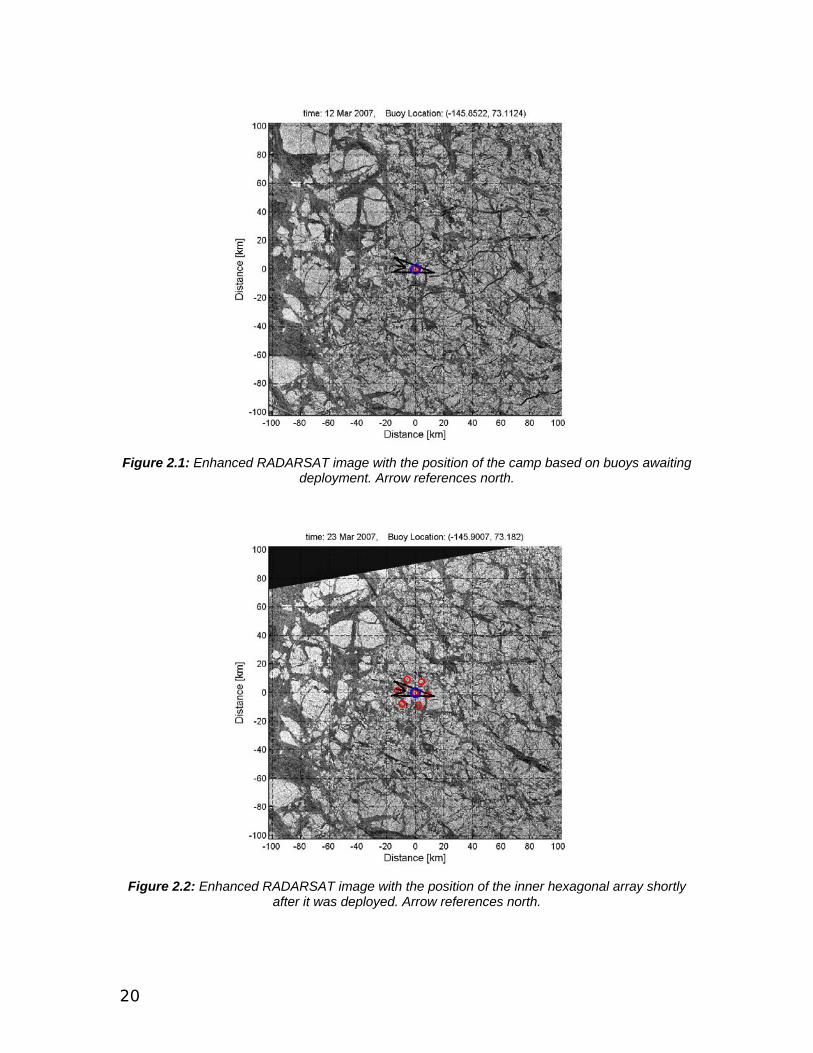
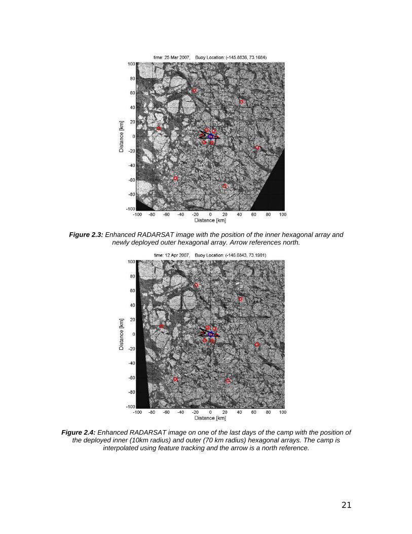
validation for both remote sensing products and models. Two important aspects of the motion algorithm used in the analysis are, i) the estimate was obtained at a resolution that is an order of magnitude greater than currently available data products (400m against 5km) and ii) discontinuities were clearly identified using a dynamic mask. It is also essential to emphasize that the motion estimates were obtained directly from the image data rather than by interpolating a coarse motion field. Discontinuous regions in the motion field were estimated using a threshold on the invariant shear extracted from the motion field. Results from the near real time motion estimate and the field visualization (using Line Integral Convolution) can be seen at http://vims.cis.udel.edu/~mani/SEDNA. The location of the camp and the deployed buoys can be observed at http://research.iarc.uaf.edu/SEDNA. The analysis was performed on a 2.93GHz, Core 2 Duo processor with a 4GB RAM. Using this configuration, image pairs with a dimension of 4096 x 4096 pixels (~200km x 200 km) were characterized for their motion content in under 3 minutes. We are currently working on improvements to analyze 500km x 1000km regions across the Arctic basin. This near-real time operational product was the first attempt at high resolution satellite motion analysis delivered operationally to a science ice camp. 2.1.2 Highlight examples Below are highlight examples of the buoy deployment as rendered using near-real time RADARSAT and real-time GPS buoy positioning. Buoy positions marked by red circle with interpolated camp marked with blue and red circle. North arrow centered over the camp. First image is from March 12 shortly after the buoys arrived at camp. Second image from 23 March just after the inner array was successfully deployed. Third image from 25 March just after the outer array successfully deployed. Forth image from 12 April at the end of the camp.

20

Figure 2.1: Enhanced RADARSAT image with the position of the camp based on buoys awaiting

deployment. Arrow references north.

Figure 2.2: Enhanced RADARSAT image with the position of the inner hexagonal array shortly

after it was deployed. Arrow references north.

21

Figure 2.3: Enhanced RADARSAT image with the position of the inner hexagonal array and

newly deployed outer hexagonal array. Arrow references north.

Figure 2.4: Enhanced RADARSAT image on one of the last days of the camp with the position of

the deployed inner (10km radius) and outer (70 km radius) hexagonal arrays. The camp is interpolated using feature tracking and the arrow is a north reference.

22

2.1.2 Near-real time motion

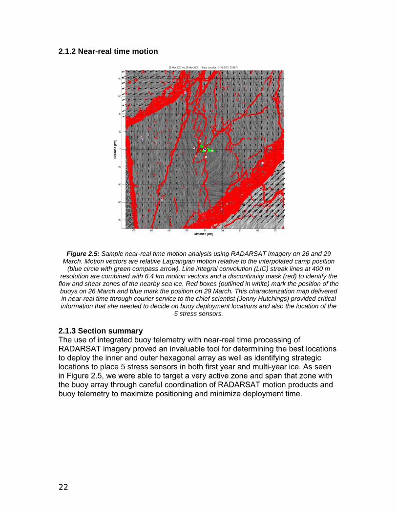
Figure 2.5: Sample near-real time motion analysis using RADARSAT imagery on 26 and 29

March. Motion vectors are relative Lagrangian motion relative to the interpolated camp position (blue circle with green compass arrow). Line integral convolution (LIC) streak lines at 400 m

resolution are combined with 6.4 km motion vectors and a discontinuity mask (red) to identify the flow and shear zones of the nearby sea ice. Red boxes (outlined in white) mark the position of the buoys on 26 March and blue mark the position on 29 March. This characterization map delivered in near-real time through courier service to the chief scientist (Jenny Hutchings) provided critical information that she needed to decide on buoy deployment locations and also the location of the

5 stress sensors. 2.1.3 Section summary The use of integrated buoy telemetry with near-real time processing of RADARSAT imagery proved an invaluable tool for determining the best locations to deploy the inner and outer hexagonal array as well as identifying strategic locations to place 5 stress sensors in both first year and multi-year ice. As seen in Figure 2.5, we were able to target a very active zone and span that zone with the buoy array through careful coordination of RADARSAT motion products and buoy telemetry to maximize positioning and minimize deployment time.

23

2.2 MODIS Nick Hughes, SAMS

2.2.1 Summary This is a report on MODIS satellite image acquisitions for the SEDNA project which covered the period between the surfacing of the submarine HMS Tireless in the area on 16 March 2007 through to the end of the ice camp on 15 April. MODIS provides a medium resolution visible image suitable for providing sea ice information during cloud-free periods. It can also be processed to yield data on surface temperature and albedo. This data is particularly useful when used in conjunction with images from SAR satellite sensors.

2.2.2 Background MODIS (or Moderate Resolution Imaging Spectroradiometer) is a key instrument aboard the Terra (EOS AM) and Aqua (EOS PM) satellites. Terra's orbit around the Earth is timed so that it passes from north to south across the equator in the morning, while Aqua passes south to north over the equator in the afternoon. Terra MODIS and Aqua MODIS are viewing the entire Earth's surface every 1 to 2 days, acquiring data in 36 spectral bands, or groups of wavelengths (see MODIS Technical Specifications). These data will improve our understanding of global dynamics and processes occurring on the land, in the oceans, and in the lower atmosphere. MODIS is playing a vital role in the development of validated, global, interactive Earth system models able to predict global change accurately enough to assist policy makers in making sound decisions concerning the protection of our environment.

2.2.3 Processing Daily raw MODIS data files (Level 1-B) in Hierarchical Data Format (HDF) were acquired for the SEDNA project for the period 15 March through to 16 April 2007. This allowed generation of quick-look images from a selection of the 36 channels available on MODIS and will allow further processing by sea ice, oceanographic and atmospheric parameter retrieval algorithms later in the SEDNA project. The data was ordered through NASA Goddard Space Flight Center (GSFC) Level 1 and Atmosphere Archive and Distribution System (LAADS Web) (http://ladsweb.nascom.nasa.gov/). The data period covers the period when the area was visited by the Royal Navy submarine HMS Tireless as part of ICEX-07 through to the end of the APLIS ice camp. The initial stage of processing was to generate single channel geo-referenced images to provide a consistent daily coverage. The projection used for SEDNA MODIS images is Polar Stereographic with a central longitude at 145°W and latitude of true scale at 90°N on the WGS84 datum. Resolution was increased to 100 metres, from the 250 metres maximum acquired by MODIS, by cubic convolution interpolation to aid comparison with the Envisat ASAR wide swath images also acquired for SEDNA. The software used was the MODIS Swath Reprojection Tool (MRT Swath) supplied by the NASA/USGS Land Processes

24

Distributed Active Archive Center (LP DAAC) (http://edcdaac.usgs.gov/landdaac/tools/mrtswath/). This takes the raw data from the HDF files and outputs single channel geo-referenced images in GeoTIFF format. This format is the result of an effort by over 160 different remote sensing, GIS, cartographic, and surveying related companies and organisations to establish an interchange format for geo-referenced raster imagery based on the common Tag Image File Format (TIFF). Further information can be found at http://remotesensing.org/geotiff/geotiff.html. GeoTIFF format was then used for all further image processing and archiving. Generation of quick-look images was performed using OpenEV software. This is an open source software library and application for viewing and analysing raster and vector geospatial data. More information on OpenEV can be found, and the software downloaded, at http://openev.sourceforge.net/. However the version used for the SEDNA MODIS images was supplied as part of the FWTools open source GIS binary kit (http://fwtools.maptools.org/) which also includes other free applications including the Geospatial Data Abstraction Library (GDAL) and the PROJ.4 cartographic projections library. The individual channel images in GeoTIFF format were loaded into OpenEV. This allows the generation of a multi-channel image through the ‘Compose’ option on the ‘Image’ menu. Three images corresponding to different channels were then selected to produce an RGB (red-green-blue) colour image corresponding to either a visible or false colour composite (FCC) quick-look image. Visible images were created using reflective channels 1, 4 and 3. These correspond to 620-670 (red), 545-565 (green), 459-479 (blue) nm (nanometre) light bandwidths. False colour composite images were created using channels 31, 2 and 3. These provide a low resolution (1,000 metre) thermal infrared image at 10.78-11.28 µm (micrometre), a high resolution (250 metre) 841-876 nm near-infrared image, and the medium resolution (500 metre) 459-479 nm (blue) visible image. This follows a method used by [Schneider and Budéus 1997] for Landsat images to improve discrimination of sea ice from open water. Cold snow and ice surfaces appear as blue and the relatively warm, thermally emitting, open water is bright red.

After composing the image in OpenEV it was exported to a GeoTIFF file. As OpenEV does not apply compression to an image this was done using the gdal_translate utility from GDAL.Image Assessment A full list of the images acquired is shown in appendix 1. A selection of some of the clearer images is presented here with a brief initial evaluation of the main features. The visible image is on the left and false colour composite on the right.

25

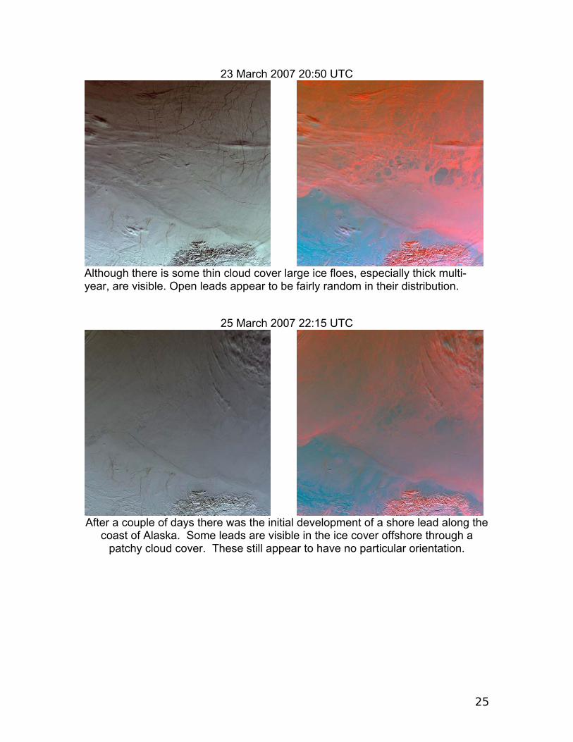
23 March 2007 20:50 UTC

Although there is some thin cloud cover large ice floes, especially thick multi-year, are visible. Open leads appear to be fairly random in their distribution.

25 March 2007 22:15 UTC

After a couple of days there was the initial development of a shore lead along the

coast of Alaska. Some leads are visible in the ice cover offshore through a patchy cloud cover. These still appear to have no particular orientation.

26

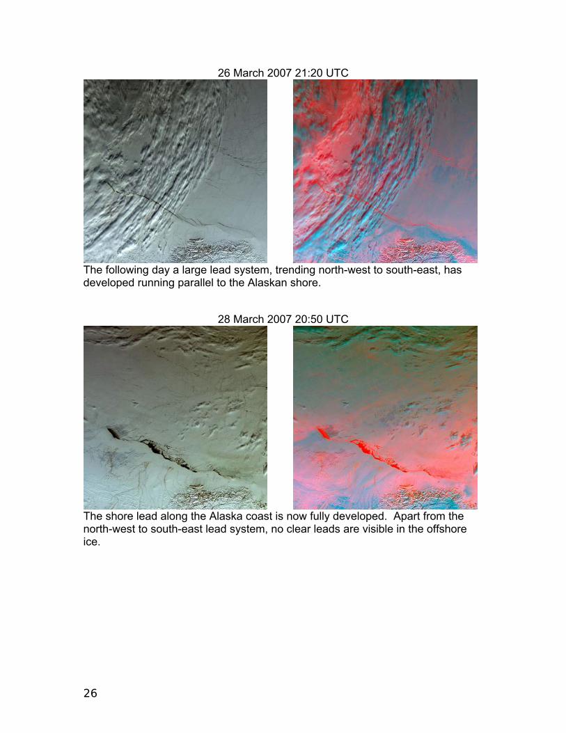
26 March 2007 21:20 UTC

The following day a large lead system, trending north-west to south-east, has developed running parallel to the Alaskan shore.

28 March 2007 20:50 UTC

The shore lead along the Alaska coast is now fully developed. Apart from the north-west to south-east lead system, no clear leads are visible in the offshore ice.

27

31 March 2007 21:20 UTC

A number of lead systems have developed. These run north-south in the northern part of the image and then trend towards the west as they run towards the shore lead.

10 April 2007 23:35 UTC

After a number of days in which cloud obscured the ice it was visible again on 8 April 2007 22:10 UTC image. During this time the ice cover continued to break up with a multitude of small leads fracturing the cover. Around Point Barrow the ice cover has broken away to start forming an embayment. Leads running north-north-west to south-south-east are dominant. These are crossed by smaller leads running north-west to south-east forming a lattice pattern. The shore lead east of Point Barrow appears to be closed

28

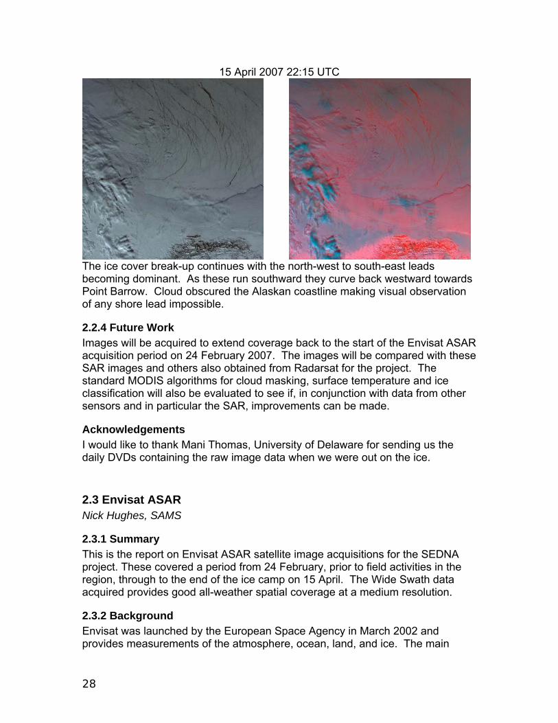
15 April 2007 22:15 UTC

The ice cover break-up continues with the north-west to south-east leads becoming dominant. As these run southward they curve back westward towards Point Barrow. Cloud obscured the Alaskan coastline making visual observation of any shore lead impossible.

2.2.4 Future Work Images will be acquired to extend coverage back to the start of the Envisat ASAR acquisition period on 24 February 2007. The images will be compared with these SAR images and others also obtained from Radarsat for the project. The standard MODIS algorithms for cloud masking, surface temperature and ice classification will also be evaluated to see if, in conjunction with data from other sensors and in particular the SAR, improvements can be made.

Acknowledgements I would like to thank Mani Thomas, University of Delaware for sending us the daily DVDs containing the raw image data when we were out on the ice.

2.3 Envisat ASAR Nick Hughes, SAMS

2.3.1 Summary This is the report on Envisat ASAR satellite image acquisitions for the SEDNA project. These covered a period from 24 February, prior to field activities in the region, through to the end of the ice camp on 15 April. The Wide Swath data acquired provides good all-weather spatial coverage at a medium resolution.

2.3.2 Background Envisat was launched by the European Space Agency in March 2002 and provides measurements of the atmosphere, ocean, land, and ice. The main

29

objective of the Envisat programme is to provide Europe with an enhanced capability for remote sensing observation of Earth from space, with the aim of further increasing the capacity of participating states to take part in the studying and monitoring of the Earth and its environment. Envisats primary objectives are: • to provide for continuity of the observations started with the ERS satellites,

including those obtained from radar-based observations; • to enhance the ERS mission, notably the ocean and ice mission; • to extend the range of parameters observed to meet the need of

increasing knowledge of the factors determining the environment; • to make a significant contribution to environmental studies, notably in the

area of atmospheric chemistry and ocean studies (including marine biology).

Envisat flies in a sun-synchronous polar orbit of about 800-km altitude. The repeat cycle of the reference orbit is 35 days, and for most sensors, being wide swath, it provides a complete coverage of the globe within one to three days. The exceptions are the profiling instruments MWR and RA-2 which do not provide real global coverage, but span a tight grid of measurements over the globe. This grid is the same 35-day repeat pattern which has been well established by ERS-1 and ERS-2. In order to ensure an efficient and optimum use of the system resources and to guarantee the achievement of the mission objectives Envisat reference mission operation profiles are established and used for mission and system analyses to define the instrument operational strategies, the command and control, and the data transmission, processing and distribution scenarios. Mission and operation requirements • Sun-synchronous polar orbit (SSO): Nominal reference orbit of mean

altitude 800 km, 35 days repeat cycle, 10:00 AM mean local solar time (MLST) descending node, 98.55 deg. inclination.

• The orbit is controlled to a maximum deviation of +/- 1 km from ground track and +/- 5 minutes on the equator crossing MLST.

• Recording of payload data over each orbit for low bit rate (4.6 Mps) on tape recorders or solid state recorder (SSR).

• High rate data (ASAR and MERIS) to be accessible by direct telemetry or recording on SSR.

A number of scenes in medium resolution (150 metre) Wide Swath mode were ordered for the APLIS ice camp to coincide with the visit by the submarine HMS Tireless and to cover the activities of the SEDNA fieldwork. Wide Swath or WSM mode provides scenes covering 406 km across-track.

2.3.3 Processing Envisat ASAR wide swath scenes were ordered from ESA in January 2007 using the EOLI SA software tool (http://eoli.esa.int/geteolisa/index.html). This provides a means of visually ensuring the correct area coverage is chosen and sends the

30

necessary ordering parameters (orbit, time, type of product, etc.) to the ESA order desk. The requests of all the users are then evaluated and tasking of the satellite takes place according to the priority given to particular users. Data is then delivered on CD- ROM or DVD after processing by various production facilities, or can be downloaded directly from the ESA Rolling Archive. Frames were processed with scripts using the Basic ERS & Envisat (A)ATSR and Meris Toolbox (BEAM). This is freely available through http://www.brockmann-consult.de/beam/ and consists of a desktop application called VISAT and a number of command line tools written in open source Java code. BEAM converts the raw ESA data format into a GeoTIFF image file. This format is an interchange format for geo-referenced raster imagery based on the common Tag Image File Format (TIFF). Further information can be found at http://remotesensing.org/geotiff/geotiff.html. GeoTIFF format was then used for all further image processing and archiving. The images were reprojected to provide a consistent coverage. The projection used for SEDNA Envisat ASAR images is Polar Stereographic with a central longitude at 145°W and latitude of true scale at 90°N on the WGS84 datum. Resolution was increased to 100 metres, from the 150 metres maximum acquired by Envisat ASAR in Wide Swath mode, by cubic convolution interpolation to aid comparison with the MODIS images also acquired for SEDNA. The gdal_translate utility provided as part of the Geospatial Data Abstraction Library (GDAL) (http://www.gdal.org/) was used to apply data compression to the GeoTIFF image. GDAL is supplied in the FWTools open source GIS binary kit (http://fwtools.maptools.org/) which also includes other free applications including OpenEV and the PROJ.4 cartographic projections library.

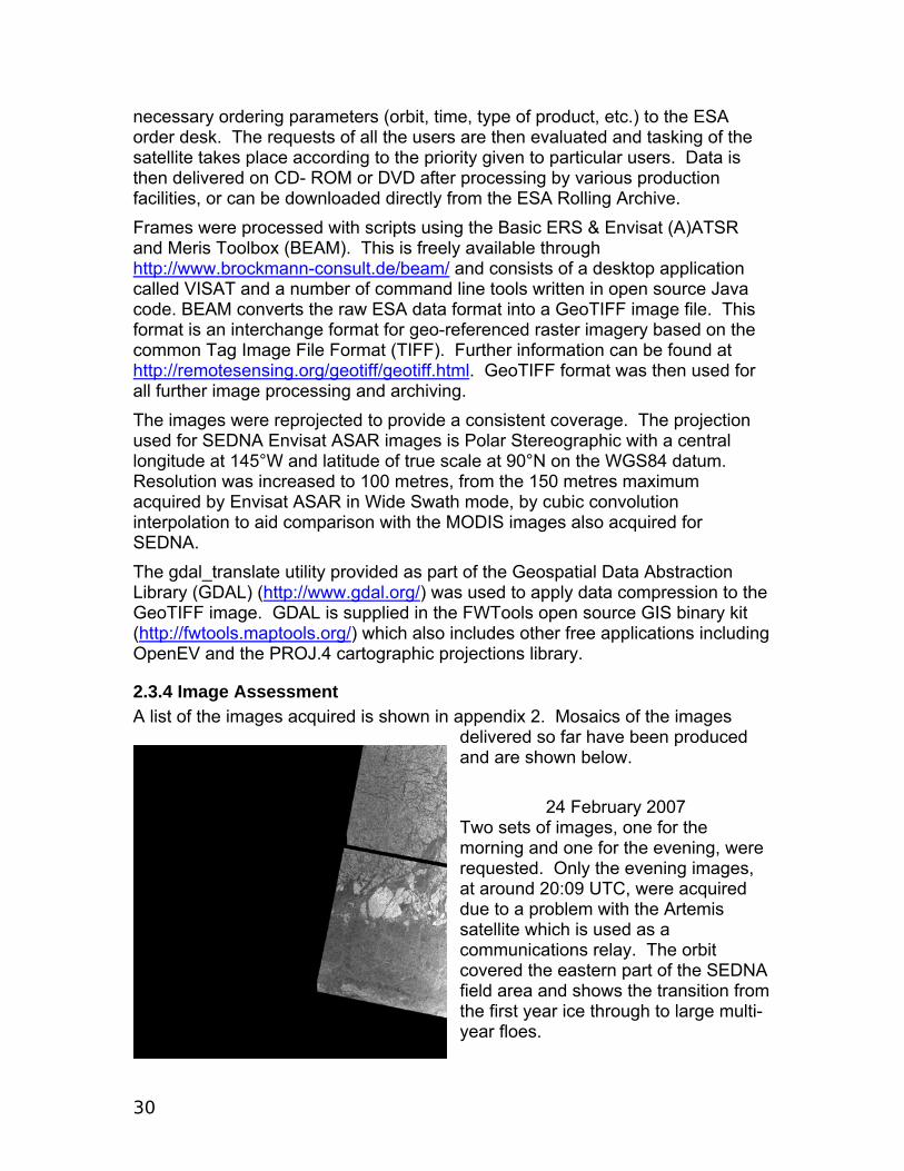
2.3.4 Image Assessment A list of the images acquired is shown in appendix 2. Mosaics of the images

delivered so far have been produced and are shown below.

24 February 2007

Two sets of images, one for the morning and one for the evening, were requested. Only the evening images, at around 20:09 UTC, were acquired due to a problem with the Artemis satellite which is used as a communications relay. The orbit covered the eastern part of the SEDNA field area and shows the transition from the first year ice through to large multi-year floes.

31

Gaps between frames exist due to insufficient overlap being requested at the time of ordering. The amount of overlap required seems to vary according to which processing centre deals with the order. The missing data can be recovered as the data from the orbit segment is held in the ESA archive.

5 March 2007

Data from a morning orbit, at 06:54 UTC, and an evening orbit, at 20:27 UTC, were acquired. These provide good coverage of the SEDNA field area with overlap in the central region of interest. This set of images also suffers from gaps

between frames.

20 March 2007 The next set of available images is from 20 March. Images were also acquired on 10 March but at the time of writing had yet to be delivered. The morning orbit occurred at 07:22 UTC and the evening orbit at 20:55 UTC. The images cover the central and western part of the SEDNA field area and occur during the time the submarine HMS Tireless was in the area conducting under-ice surveys. Image frames from these orbits are continuous with no gaps.

32

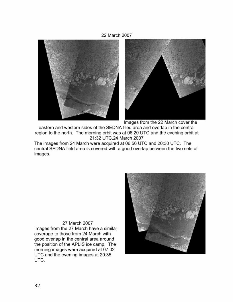
22 March 2007

Images from the 22 March cover the eastern and western sides of the SEDNA filed area and overlap in the central

region to the north. The morning orbit was at 06:20 UTC and the evening orbit at 21:32 UTC.24 March 2007

The images from 24 March were acquired at 06:56 UTC and 20:30 UTC. The central SEDNA field area is covered with a good overlap between the two sets of images.

27 March 2007 Images from the 27 March have a similar coverage to those from 24 March with good overlap in the central area around the position of the APLIS ice camp. The morning images were acquired at 07:02 UTC and the evening images at 20:35 UTC.

33

Further images were acquired, as listed in appendix 2. Delivery of these is on-going and will be reported on in a later report.

2.3.5 Future Work Once delivery of images is complete and any gaps in coverage recovered the images will be compared with MODIS images of the area and other SAR images obtained from Radarsat for the project. Various methods for classifying SAR images for sea ice will be evaluated to see if, in conjunction with data from other sensors and in particular MODIS, improvements can be made.

Acknowledgements The Envisat ASAR images were acquired as part of Professor Peter Wadham’s ESA Envisat Announcement of Opportunity project #208 ‘The Use of ASAR, AATSR and Altimeter Data Products for the study of Sea Ice Response to Climatic Change’. 2.4 Envisat RA-2 measurements over the SEDNA ice camp Katharine Giles, University Collage London For the duration of the ice camp (1st to 14th April) data from the radar altimeter (RA-2) onboard the European Space Agency Satellite (ESA) Envisat, was used to calculate the sea ice freeboard over the camp and surrounding ice. Altimeters measure the two way travel time of a pulse of radiation from the instrument to the surface, and use this to calculate the elevation of the surface above a reference surface. The technique used to calculate sea ice freeboard utilises the fact that different radar returns are received over sea ice and over leads, therefore allowing us to distinguish between the ice elevation and the ocean elevation. Sea ice freeboard can then be calculated by subtracting the ice elevation from the ocean elevation (Laxon et al., 2003, Peacock & Laxon, 2004). Figure 2.6 show a selection of days of Envisat freeboard estimates with the camp location shown by the red triangles. The three examples in figure 2.6 were chosen to show those days where there were a relatively large proportion of RA-2 freeboard estimates very close to the ice camp (b and c) and the day with the lowest amount of coincident data (c). The average offset between the camp location and the centre of the closet freeboard estimate is 135 km1. As radar returns are noisy, the satellite data have been averaged to produce the freeboard estimates shown in figure 2.6. Each point represents the integrated response of the radar over a distance of 2-5 Km, depending on the surface roughness.

1 This average includes all of the data, 18th March to the 15th April.

34

Figure 2.6: Examples of the freeboard estimates derived from RA-2 data during the SEDNA ice camp. The red triangle marks the position of the ice camp. There are gaps in the satellite data as freeboard estimates can only be made when the whole of the radar footprint is filled with consolidated sea ice. In a) SEDNA is located at a latitude of 73.171930� N and longitude of -145.833447� W, and the centre of the nearest RA-2 freeboard estimate is 324 km away. In b) SEDNA is located at a latitude of 73.299722� N and longitude of -145.408895� W, and the centre of the nearest RA-2 freeboard estimate is 25 km away. In c) SEDNA is located at a latitude of 73.189283� N and longitude of -146.699528� W, and the centre of the nearest RA-2 freeboard estimate is 26 km away. Ideally, to validate estimates of ice freeboard, the ice needs to be surveyed over the averaging area of the estimate. However, the data latency between the satellite acquiring the data, and the data being delivered by ESA to the Centre for Polar Observation and Modelling (CPOM), University College London, for

35

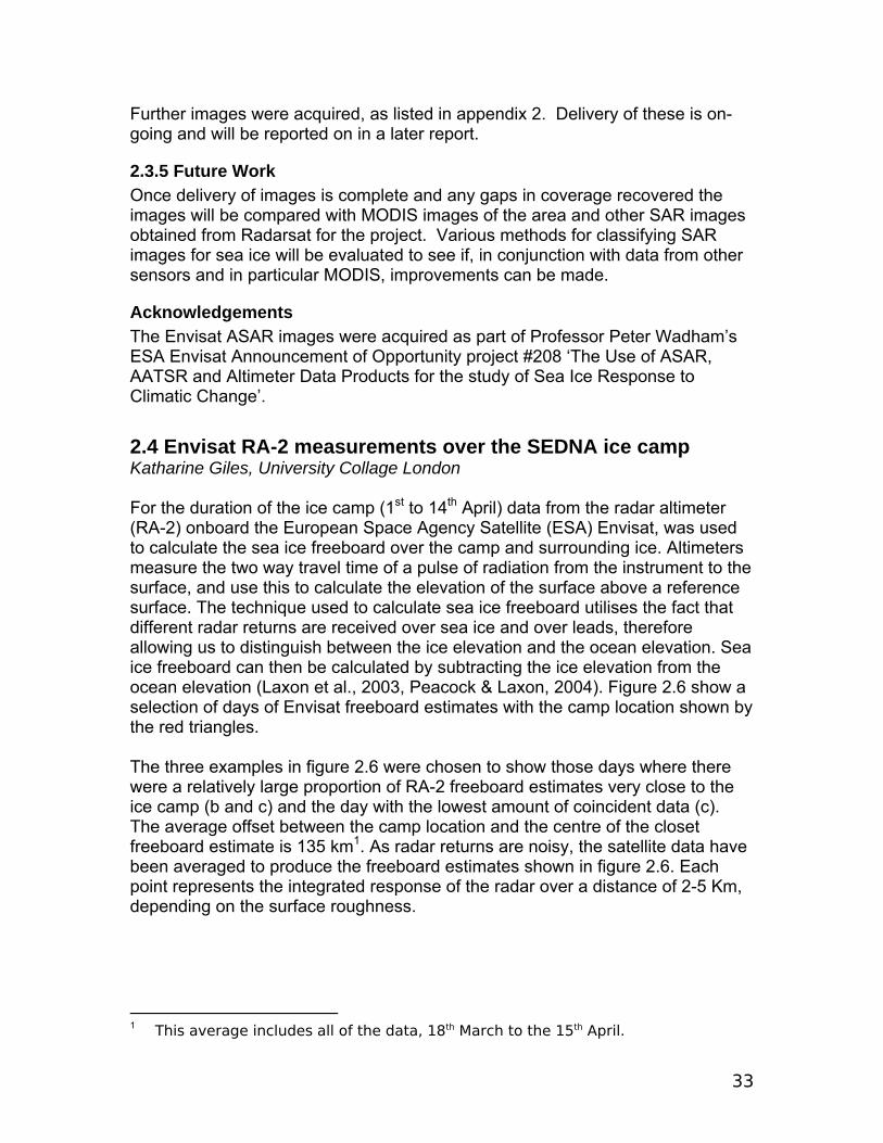
freeboard processing, is about 5 days2. Therefore, once the data has been processed and areas of ice freeboard estimates identified, one must estimate how much the ice has moved since the satellite measurements were taken (5 days) and then survey the shifted ice. The likelihood of the surveying the same ice measured by the satellite could be improved by: (1) shortening the data latency, this is a recommendation we plan to discuss with ESA; (2) improving the freeboard processing algorithm to reduce the data gaps, thereby increasing the chance that an area of ice that has been surveyed will match the location of a freeboard estimate. Improving the freeboard processing algorithm is an on going process at CPOM. Figure 2.6 shows the potential for using near real-time satellite data to locate satellite validation sites. To validate the satellite measurements we would envisage surveying an area where we have a series of freeboard estimates close to the camp, such as in figure 2.6(c), using primarily airborne surveys (e.g. EM bird towed by a helicopter and airborne altimetry measurements). Acknowledgements Andy Ridout and Seymour Laxon, from CPOM, for processing and sending the freeboard estimates to the ice camp. ESA for the Intermediate Special Geophysical Data Record. 2.5 IceSat Jay Zwally & Cathleen Geiger Jay Zwally, and the NASA IceSat team, arranged for the spring 2007 IceSat mission to be shifted 16 days later than planned. This ensured IceSat could provide coverage of the Arctic during the entire time period of the APLIS 2007 ice camp. The IceSat mission ran from March 12th until April 14th 2007. We had hoped that an IceSat orbit would fall within survey distance of the ice camp. Survey distance was the range of the Bell 212 helicopter, and an orbit would have to have fallen within 100km of the ice camp to allow sufficient survey length along the track with EM-bird. Due to the short duration of the ice camp (2 weeks), the possibility of surveying an IceSat orbit was small. Figure 2.7 shows orbits that fell in the Beaufort Sea during the ice camp. The green line shows the camp track, with dates labeled as julian days. The dates of each orbit are labeled along the top of the plot. Only the orbit on day 84 (March 14th) came close to the camp. Rene Forsberg attempted to survey the March 14th orbit on April 12th by Twin Otter.

2 Once the data has arrived at CPOM, it can be processed in less than a day.

36

Figure 2.7: IceSat Orbits, red dotted lines, superimposed on the ice camp track, green solid line. Dates on the camp track, corresponding to orbit date, are labeled as Julian Days. Orbit dates are labeled along the top of the plot.

2.6 ALOS PALSAR and ERS-2 SAR Imagery Ben Holt, JPL This section summarizes additional SAR imagery obtained during the SEDNA project. ALOS PALSAR was obtained through requests to the ALOS America Data Node at the Alaska Satellite Facility (ASF), to support an approved ALOS data proposal. PALSAR is an L-band SAR (1.2 GHz) with several modes including fine beam, polarimetry and wide swath modes over multiple incidence angles. This sensor is operated by the Japanese Space Agency JAXA. ERS-2 SAR data was also requested through ASF. This SAR operates at C-band frequency (5.4 GHz) with a 25 m resolution and a 100 km swath width at a fixed single range of incidence angles. Both data sets will provide finer resolution capabilities over the camp region than that available from Radarsat however with reduced spatial and temporal sampling. Figure 1 provides examples of all three sensors over the camp region and illustrates the different radar response between C-band and L-band particularly with respect to ice types and deformed ice. To obtain any of these data, please contact ben.holt@jpl.nasa.gov directly or ASF (asf.alaska.edu). 2.6.1 ALOS PALSAR

37

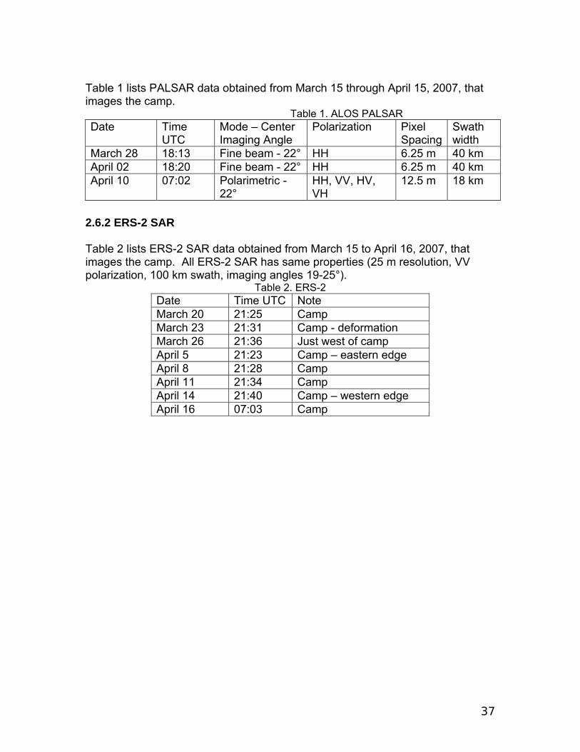
Table 1 lists PALSAR data obtained from March 15 through April 15, 2007, that images the camp. Table 1. ALOS PALSAR Date Time

UTC Mode – Center Imaging Angle

Polarization Pixel Spacing

Swath width

March 28 18:13 Fine beam - 22° HH 6.25 m 40 km April 02 18:20 Fine beam - 22° HH 6.25 m 40 km April 10 07:02 Polarimetric -

22° HH, VV, HV, VH

12.5 m 18 km

2.6.2 ERS-2 SAR Table 2 lists ERS-2 SAR data obtained from March 15 to April 16, 2007, that images the camp. All ERS-2 SAR has same properties (25 m resolution, VV polarization, 100 km swath, imaging angles 19-25°).

Table 2. ERS-2 Date Time UTC Note March 20 21:25 Camp March 23 21:31 Camp - deformation March 26 21:36 Just west of camp April 5 21:23 Camp – eastern edge April 8 21:28 Camp April 11 21:34 Camp April 14 21:40 Camp – western edge April 16 07:03 Camp

38

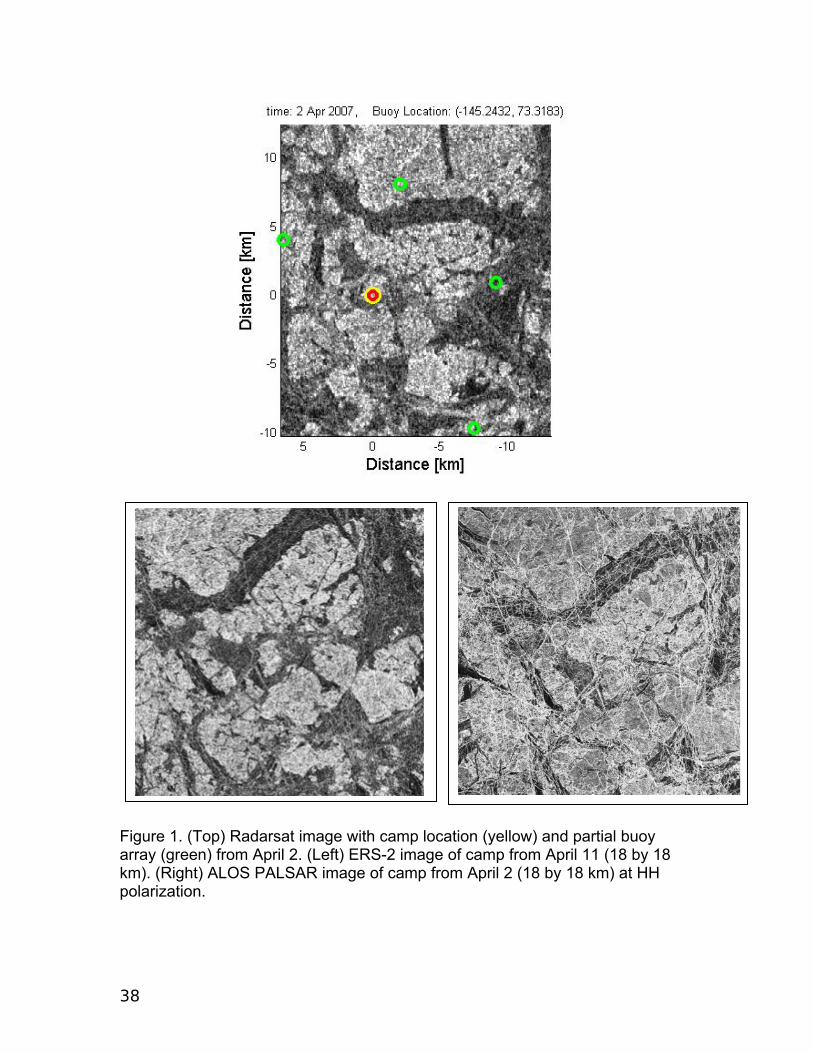
Figure 1. (Top) Radarsat image with camp location (yellow) and partial buoy array (green) from April 2. (Left) ERS-2 image of camp from April 11 (18 by 18 km). (Right) ALOS PALSAR image of camp from April 2 (18 by 18 km) at HH polarization.

39

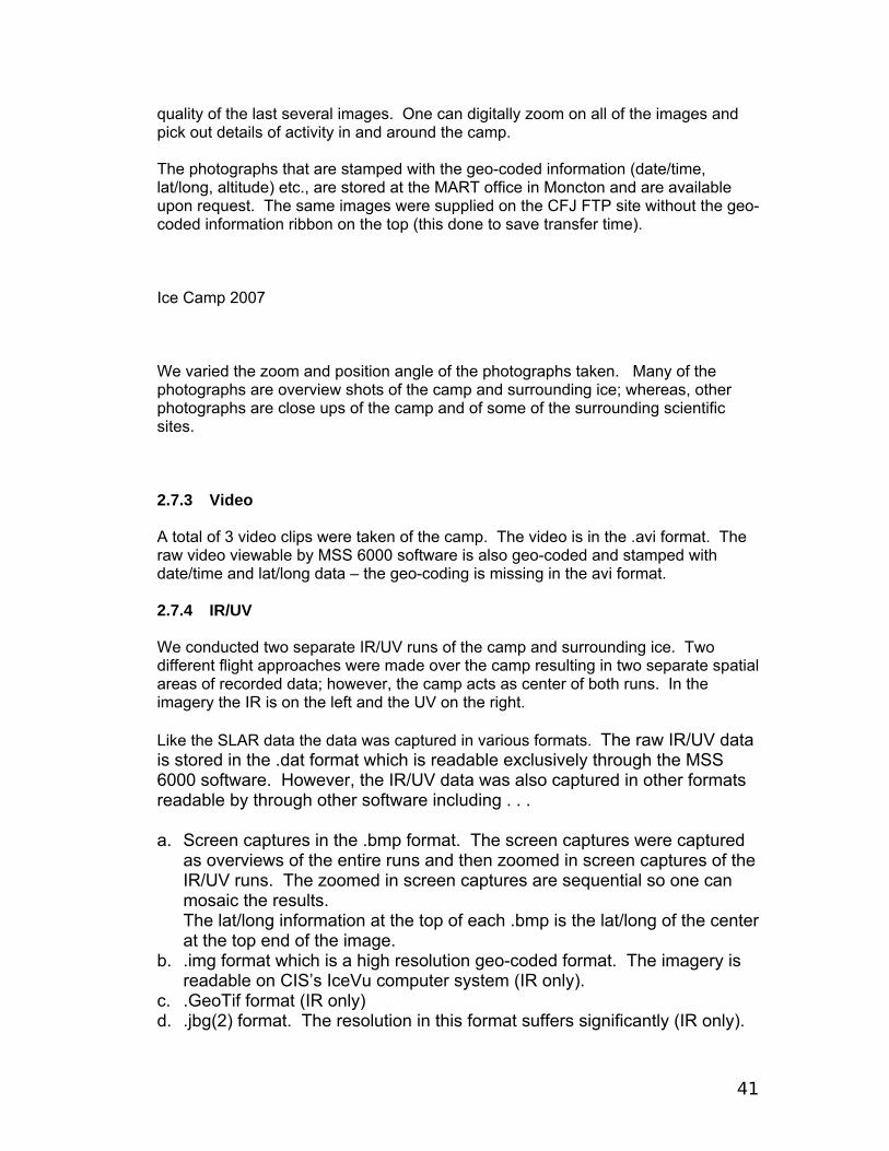
2.7 Report on mission by C-GCFJ, DASH 8 Mac McGregor On 02 April 2007, C-GCFJ (Dash 8) was tasked to support Ice Camp 2007 situated at approximately 7321N 14517W. We flew high level from Fairbanks Alaska and picked up our track at Prudhoe Bay at which point we commenced reconnaissance of ice conditions from the shore to the camp. The following data captures were completed as part of this mission

2.7.1 Side Looking Airborne Radar

This SLAR is manufactured by Ericson that operates on X-band and produces 60 metre resolution imagery.

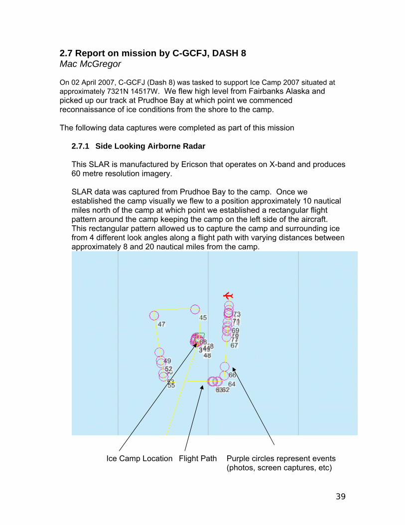
SLAR data was captured from Prudhoe Bay to the camp. Once we established the camp visually we flew to a position approximately 10 nautical miles north of the camp at which point we established a rectangular flight pattern around the camp keeping the camp on the left side of the aircraft. This rectangular pattern allowed us to capture the camp and surrounding ice from 4 different look angles along a flight path with varying distances between approximately 8 and 20 nautical miles from the camp.

Ice Camp Location Flight Path Purple circles represent events (photos, screen captures, etc)

40

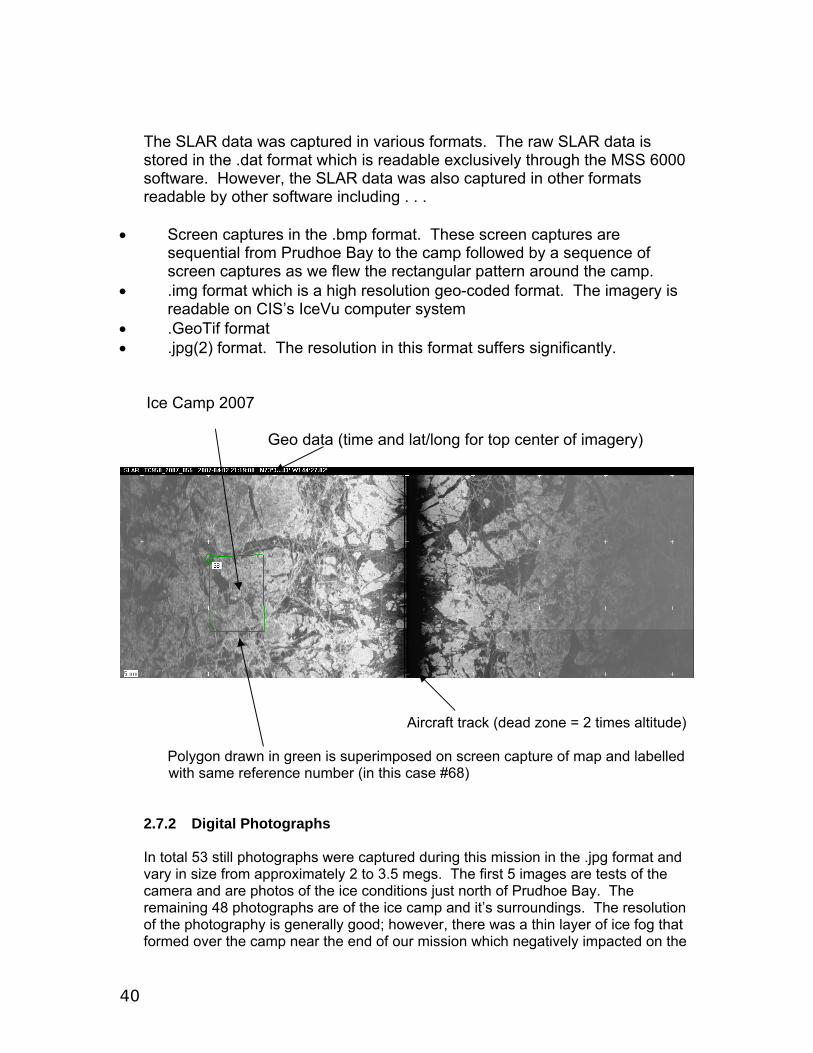
The SLAR data was captured in various formats. The raw SLAR data is stored in the .dat format which is readable exclusively through the MSS 6000 software. However, the SLAR data was also captured in other formats readable by other software including . . .

• Screen captures in the .bmp format. These screen captures are sequential from Prudhoe Bay to the camp followed by a sequence of screen captures as we flew the rectangular pattern around the camp.

• .img format which is a high resolution geo-coded format. The imagery is readable on CIS’s IceVu computer system

• .GeoTif format • .jpg(2) format. The resolution in this format suffers significantly. Ice Camp 2007 Geo data (time and lat/long for top center of imagery)

Aircraft track (dead zone = 2 times altitude) Polygon drawn in green is superimposed on screen capture of map and labelled with same reference number (in this case #68)

2.7.2 Digital Photographs

In total 53 still photographs were captured during this mission in the .jpg format and vary in size from approximately 2 to 3.5 megs. The first 5 images are tests of the camera and are photos of the ice conditions just north of Prudhoe Bay. The remaining 48 photographs are of the ice camp and it’s surroundings. The resolution of the photography is generally good; however, there was a thin layer of ice fog that formed over the camp near the end of our mission which negatively impacted on the

41

quality of the last several images. One can digitally zoom on all of the images and pick out details of activity in and around the camp. The photographs that are stamped with the geo-coded information (date/time, lat/long, altitude) etc., are stored at the MART office in Moncton and are available upon request. The same images were supplied on the CFJ FTP site without the geo-coded information ribbon on the top (this done to save transfer time). Ice Camp 2007 We varied the zoom and position angle of the photographs taken. Many of the photographs are overview shots of the camp and surrounding ice; whereas, other photographs are close ups of the camp and of some of the surrounding scientific sites. 2.7.3 Video

A total of 3 video clips were taken of the camp. The video is in the .avi format. The raw video viewable by MSS 6000 software is also geo-coded and stamped with date/time and lat/long data – the geo-coding is missing in the avi format. 2.7.4 IR/UV

We conducted two separate IR/UV runs of the camp and surrounding ice. Two different flight approaches were made over the camp resulting in two separate spatial areas of recorded data; however, the camp acts as center of both runs. In the imagery the IR is on the left and the UV on the right. Like the SLAR data the data was captured in various formats. The raw IR/UV data is stored in the .dat format which is readable exclusively through the MSS 6000 software. However, the IR/UV data was also captured in other formats readable by through other software including . . . a. Screen captures in the .bmp format. The screen captures were captured

as overviews of the entire runs and then zoomed in screen captures of the IR/UV runs. The zoomed in screen captures are sequential so one can mosaic the results. The lat/long information at the top of each .bmp is the lat/long of the center at the top end of the image.

b. .img format which is a high resolution geo-coded format. The imagery is readable on CIS’s IceVu computer system (IR only).

c. .GeoTif format (IR only) d. .jbg(2) format. The resolution in this format suffers significantly (IR only).

42

Ice Camp (IR left, UV right)

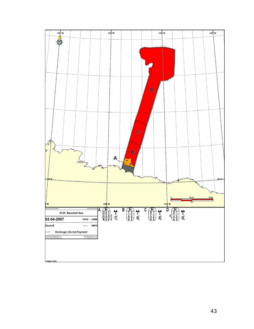
2.7.5 Visual Ice Chart

A visual ice chart of the ice conditions from Prudhoe Bay to and around the camp was constructed. The ice is coded in standard Ice Egg code. This chart was saved as a .gif file so that it could be readable by most standard viewers.Visual Ice Reconnaissance Chart – 02 April 2007

43

44

2.7.6 MX-15 Data

Throughout our time on site we actively used the MX-15 to observe the camp and surrounding ice and activity on the ice. We activated all three modes of this sensor including Electric Optical Wide (EOW), Electric Optical Narrow (EON) and Infra Red (both NIR and IR). This sensor had not yet been fully integrated into the MSS 6000 and as such we were unable to record any of this data.

2.7.7 Data Storage All data in the various formats has been archived and is stored at the Marine Aerial Reconnaissance Team (MART) Atlantic office in Moncton New Brunswick. Excerpts of this data set that would be readable by most commercial software viewers has been place in the CFJ ftp site under the folder Ice Camp 2007 This data does not include the .dat format readable by the MSS 6000 software; however, the .dat data is available upon request.

45

3. Buoy Deployments

Buoys were deployed as early as possible during March and April 2007, in an array about the ice camp. The array was embedded into the International Arctic Buoy Program buoy distribution, and was designed to monitor ice pack deformation over 20km, 140km and regional scales. Stress buoys were deployed at 10km about camp, and these monitor stress propagation through the pack ice over a variety of scales. An ice mass balance buoy was deployed at the ice camp, providing information about thermodynamic changes to the ice pack. Additionally two SAMS tilt meter buoys were deployed, which may be used to estimate regional ice thickness. Five buoys were deployed for the IABP. 3.1 GPS buoy deployments Jennifer Hutchings Randy Ray and Doug Anderson, both from the Arctic Submarine Laboratory, assisted in early deployment of 12 GPS-ARGOS ice drifting buoys in two hexagons about the ice camp. The buoys were Oceanetic Measurement, model 406, with Trimble Lassen IQ, 12 channel, GPS engines. 12 buoys were deployed in two nested hexagon arrays. The inner ring of buoys was deployed on March 23, with a radius of 10km. The outer, 70km radius ring, was deployed on March 24. All buoys were placed on multi-year ice, paying attention to choosing sites that were older than surrounding ice. Deployment position relative to camp

10km array buoy (ARGOS ID)

70km array buoy (ARGOS ID)

North 74358 74360 North-East-East 74359 74361 South-East-East 74363 74357 South 74364 74362 South-West-West 74356 74355 North-West-West 74354 74353

Table 3.1: Directions from camp in which buoys where deployed.

46

150 W

150 W

148 W

148 W

146 W

146 W

144 W

144 W

142 W

142 W

72 00 N72 00 N

72 12 N72 12 N

72 24 N72 24 N

72 36 N72 36 N

72 48 N72 48 N

73 00 N73 00 N

73 12 N73 12 N

73 24 N73 24 N

73 36 N73 36 N

73 48 N73 48 N

74 00 N74 00 N

150 W

150 W

148 W

148 W

146 W

146 W

144 W

144 W

142 W

142 W

72 00 N72 00 N

72 12 N72 12 N

72 24 N72 24 N

72 36 N72 36 N

72 48 N72 48 N

73 00 N73 00 N

73 12 N73 12 N

73 24 N73 24 N

73 36 N73 36 N

73 48 N73 48 N

74 00 N74 00 N

150 W

150 W

148 W

148 W

146 W

146 W

144 W

144 W

142 W

142 W

72 00 N72 00 N

72 12 N72 12 N

72 24 N72 24 N

72 36 N72 36 N

72 48 N72 48 N

73 00 N73 00 N

73 12 N73 12 N

73 24 N73 24 N

73 36 N73 36 N

73 48 N73 48 N

74 00 N74 00 N

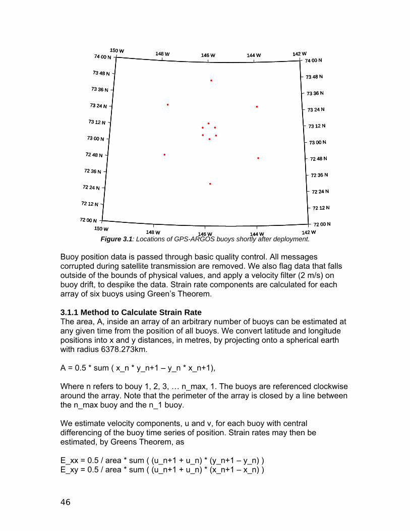
Figure 3.1: Locations of GPS-ARGOS buoys shortly after deployment.

Buoy position data is passed through basic quality control. All messages corrupted during satellite transmission are removed. We also flag data that falls outside of the bounds of physical values, and apply a velocity filter (2 m/s) on buoy drift, to despike the data. Strain rate components are calculated for each array of six buoys using Green’s Theorem. 3.1.1 Method to Calculate Strain Rate The area, A, inside an array of an arbitrary number of buoys can be estimated at any given time from the position of all buoys. We convert latitude and longitude positions into x and y distances, in metres, by projecting onto a spherical earth with radius 6378.273km. A = 0.5 * sum ( x_n * y_n+1 – y_n * x_n+1), Where n refers to bouy 1, 2, 3, … n_max, 1. The buoys are referenced clockwise around the array. Note that the perimeter of the array is closed by a line between the n_max buoy and the n_1 buoy. We estimate velocity components, u and v, for each buoy with central differencing of the buoy time series of position. Strain rates may then be estimated, by Greens Theorem, as E_xx = 0.5 / area * sum ( (u_n+1 + u_n) * (y_n+1 – y_n) ) E_xy = 0.5 / area * sum ( (u_n+1 + u_n) * (x_n+1 – x_n) )

47

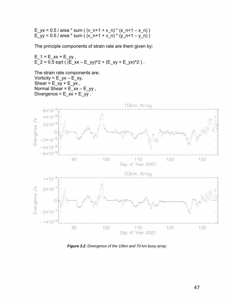
E_yx = 0.5 / area * sum ( (v_n+1 + v_n) * (x_n+1 – x_n) ) E_yy = 0.5 / area * sum ( (v_n+1 + v_n) * (y_n+1 – y_n) ) The principle components of strain rate are them given by: E_1 = E_xx + E_yy , E_2 = 0.5 sqrt ( (E_xx – E_yy)^2 + (E_xy + E_yx)^2 ) . The strain rate components are: Vorticity = E_yx – E_xy, Shear = E_xy + E_yx , Normal Shear = E_xx – E_yy , Divergence = E_xx + E_yy .

Figure 3.2: Divergence of the 10km and 70 km buoy array.

48

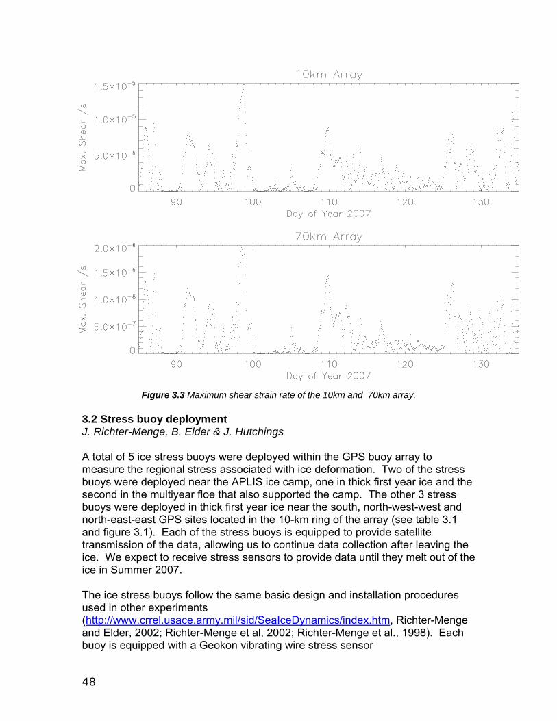
Figure 3.3 Maximum shear strain rate of the 10km and 70km array.

3.2 Stress buoy deployment J. Richter-Menge, B. Elder & J. Hutchings A total of 5 ice stress buoys were deployed within the GPS buoy array to measure the regional stress associated with ice deformation. Two of the stress buoys were deployed near the APLIS ice camp, one in thick first year ice and the second in the multiyear floe that also supported the camp. The other 3 stress buoys were deployed in thick first year ice near the south, north-west-west and north-east-east GPS sites located in the 10-km ring of the array (see table 3.1 and figure 3.1). Each of the stress buoys is equipped to provide satellite transmission of the data, allowing us to continue data collection after leaving the ice. We expect to receive stress sensors to provide data until they melt out of the ice in Summer 2007. The ice stress buoys follow the same basic design and installation procedures used in other experiments (http://www.crrel.usace.army.mil/sid/SeaIceDynamics/index.htm, Richter-Menge and Elder, 2002; Richter-Menge et al, 2002; Richter-Menge et al., 1998). Each buoy is equipped with a Geokon vibrating wire stress sensor

49

(http://www.geokon.com/products/datasheets/4300.pdf; Cox and Johnson, 1983), frozen into the ice cover at a depth that is near the top of the ice cover, but below freeboard. These sensors are designed to provide measurements of the magnitude and direction of the major and minor principal stresses in the ice cover. Other instruments on the buoy provide information on the location of the buoy, surface air temperature and sea level pressure. New to this series of buoys is the installation of a compass to measure the rotation of the buoy. With the compass we look to establish a reference system for determining the principal stress direction relative to the driving forces and deformation fields. In previous experiments, we have deployed the stress sensors in the fall. This necessitated that the buoys be located in multiyear ice, understanding that the inherent non-uniformity in the thickness and ice structure characteristics of the of this ice type complicate the interpretation of the data. Working from the APLIS 2007 ice camp provided the first opportunity to establish the ice stress measurements in thick first year ice. Knowing that the thick first year ice has more uniform characteristics than multiyear ice and, since it is thinner than the multiyear ice, may concentrate the stress signal we decided to take advantage of this situation and deployed most of the sensors in thick first year ice. The one sensor located in the multiyear ice floe that support the APLIS base camp will help us assess these assumptions and provide continuity with our previous stress data. 3.3 Ice Mass Balance Buoy (IMB) J. Richter-Menge & B. Elder An IMB was also deployed as part of the SEDNA experiment to monitor thermodynamically-driven changes in the mass balance of the sea ice cover. As described in Richter-Menge et al. (2006), the IMB is an autonomous instrument package equipped with sensors to measure snow accumulation and ablation, ice growth and melt, and internal ice temperature plus a satellite transmitter. The IMB is unique in its ability to determine whether changes in the thickness of the ice cover occur at the top or bottom of the ice cover and, hence, provide insight on the driving forces behind the change. The IMB buoys are also equipped to measure position (via ARGOS), sea level pressure , and surface air temperature. The SEDNA IMB was deployed on 8 April on the floe that served as a base for the APLIS Ice Camp. It was installed in a region of undeformed multiyear ice. Data from the IMB can be retrieved at http://www.crrel.usace.army.mil/sid/IMB/index.htm. 3.4 Tilt Meter Buoys Jeremy Wilkinson The Arctic is warming faster than any other region of the globe. Over the past few decades this warming has been accompanied by a reduction of perennial ice

50

within the Arctic Basin; a decrease in the extent of sea ice of about 15% as well as a decline by some 40% in the thickness of summer sea ice. Moreover, accelerated change is predicted including a temperature rise of more than 4ºC over the next 50 years and the disappearance of summer sea ice by 2040. The disappearance of summer sea ice in the Arctic is a climatic event that has not been seen before. If predictions prove right, and later the century the Arctic does indeed become ice free, then this change will have enormous consequences on both the local and global environment, as well as the associated socio-economic impacts affecting human beings, human health and human activities. The Arctic Ocean represents one of the most serious challenges for the monitoring and measurement of the physical environment. One of the hardest parameters to obtain on a synoptic scale is the measurement of sea ice thickness. This can only be achieved with satellite-mounted sensors; however there are at present no sensors that can measure the thickness of sea ice directly. The only satellite-borne technique that shows promise is radar and laser altimetry, which measures the height of the sea ice above the ocean’s surface, this is known as freeboard. However this technique uses a number of broad assumptions to change ice freeboard to ice thickness, and has not yet been fully validated in comparative experiments. Other satellite-based techniques using SAR or passive microwave involve inference of ice thickness from other measured parameters. Airborne techniques (laser altimetry for freeboard; electromagnetic sounding for thickness) are expensive for obtaining data over large areas, while through-ice techniques (hole drilling, surface sounding) are purely local. At present the only way to map the sea ice thickness over large regions is with upward looking sonars mounted on nuclear powered submarines. Due to military operations most parts of the Arctic Ocean have now been mapped at various times by under-ice sonar. It is from the sonar profiling of the sea ice during these missions that the main information on sea ice thinning over the past decades has come. However with the end of the Cold war the deployment of British and US submarines in the Arctic has become more sporadic and their operations have been severely reduced in scope. The number of submarines obtaining ice thickness data from the Arctic has diminished to the point where we are no longer acquiring enough data to show us what spatial and temporal trends are occurring. Until satellite sensors are able to obtain accurate ice thickness data we need another method to obtain continuous, synoptic, and long-term monitoring of ice thickness. Recently developed theory suggests that the propagation of flexural-gravity waves in ice have a spectral peak at a frequency which is a function of ice thickness. In other words, if we measure the oscillation spectrum on the ice

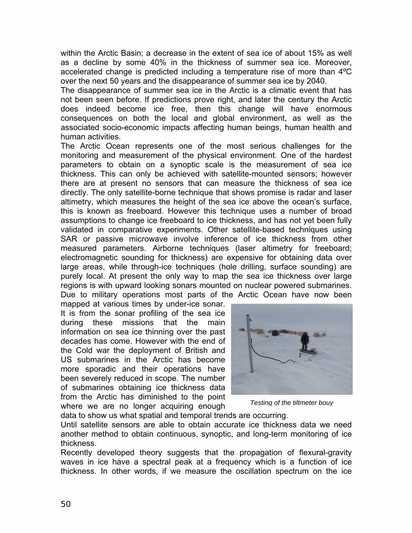
Testing of the tiltmeter bouy

51

surface, we can derive information on ice thickness. In fact this technique has the potential to measure and monitor the evolution of the modal multiyear ice thickness along the whole wave propagation path, from the open ocean to the measurement site. Flexural gravity waves originate as open ocean swell in the Greenland Sea, but evolve as they cross they pass through sea ice into a spectrum where the peak energy is concentrated at longer periods, usually around 30 seconds. These tiny oscillations can be detected in the central Arctic by very sensitive instruments such as tiltmeters and strainmeters. For decades sea-ice researchers have used different methods to measure the propagation of waves, originating from ocean swell, through sea ice. Most of these instruments were delicate to transport, maintain and labour intensive to install. Furthermore they required constant attention to ensure that the sensors were always in range, and due to the relatively high recording frequency, data was recorded internally. This in turn demanded that the instrument be revisited for data recovery. Recently scientists from the Scottish Association for Marine Science in partnership with the University of Cambridge developed an autonomous system to measure and transmit information on the propagation of flexural gravity waves in sea ice. During our participation in the APLIS/SEDNA ice camp we were able to deploy 2 of these systems in the Beaufort Sea region of the Arctic Ocean (D10 and D14). A further 3 were deployed as part of the EU funded DAMOCLES programme; one at the North Pole (D11); one east of the North Pole (D9); and one between Greenland and the North Pole (D12). This enabled good coverage of the entire Arctic Ocean with respect to gravity wave propagation. The following shows the location of the buoys at the start of the experiment. Details are summarised in table 3.2. Buoy

ID Date Latitude

(deg) Longitude

(deg) Distance to

ice edge (km)

Mechanism for Deployment

D12 30th April 84.6 -1.1 ~1000 Twin Otter landing on sea ice D11 24th April 89.5 139.5 ~1400 Twin Otter landing on sea ice near

NP D 9 24th April 87.8 129.6 ~1600 Deployed at TARA ice camp D14 9th April 74.7 -146.6 ~3000 Helicopter landing on sea ice D10 10th April 73.2 -146.7 ~3200 Deployed at SEDNA ice camp Table 3.2. Table showing the deployment details for each buoy. Also included is the distance from the ice edge to each buoy. The table is arranged with respect to distance to the ice edge i.e. buoy closest to the ice edge at the top of the table.

52

3.5 IABP deployments Ignatius Rigor, Pablo Clemente-Colon, Bruce Elder and Jennifer Hutchings Three Met Ocean ice beacons were deployed, each 100 miles from the ice camp, to the North, East and West. They fill in gaps in the IABP buoy distribution, and will provide improvements to estimates of large scale meteorological and ice motion data in the region. Each beacon measures sea level pressure and surface air temperature (at 2m). They are designed to float. Data from these is being streamed onto the WMO GTS, hence the buoys are included in routine weather analyses and reanalyses. This was the first deployment of these buoys by helicopter. Some problems with the Met Ocean design were discovered. Namely 1) The buoy can not be transported in an active state by Bell 212 helicopter, as the 2m mast does not in fit the aircraft. 2) A variety of small nuts and bolts make it very difficult to assemble the buoy in extreme cold conditions. Bruce Elder has addressed these issues with the manufacture. Two SVP buoys were also deployed. These are being tested by the International Arctic Buoy Program for Arctic use. IABP is also investigating if the sea surface temperature sensor on the SVP buoy provides useful information on sea ice. One was placed next to the Ice Mass Balance buoy, allowing validation of the temperature sensor data and investigation of how this relates to SAT. Another was placed in an active lead, to observe how it responded to ice deformation forces and refreezing. This buoy stopped reporting shortly after a ridging event in the lead, and we were unable to relocate the buoy to investigate the damage. 3.6 High density buoy deployment Cathleen Geiger, Mani Thomas & Jennifer Hutchings Seven high temporal sampling (10 second interval) non-telemetry buoys were deployed across a highly deformed area spanning roughly 7 km in anticipation of a large shear event. The large shear event did not occur but layout enabled us to characterize different types of motion to test elements of a high resolution SAR processing system. The instruments were without telemetry but were pulled together as an extra set of GPS units intended for validation points and quality control studies. The cluster was arranged into two sub-clusters in groups of 4 and 3 (Figure 3.4) with the group of 4 spanning a slowly deforming small and local ridge event to test the finescale tracking capabilities of the SAR at high resolution (cluster of 4 closest to the camp). The second cluster was located along a multi-year floe edge right next to a refrozen lead to test characterizations of backscatter, tracking, and speckle effects. In combination (Figures 3.5&3.6), the collection of highly clustered buoys together with the 10 km hexagonal array will be used to characterize a hierarchy of motion types in detail from 10 km down to 400 m to test the processing of the SAR motion tracking system used in this field

53

experiment. Example figures provided below.

Figure 3.4: Position of a non-telemetry high density array of 7 buoys deployed on either side of a highly deformed region. The cluster of 4 buoys spanning a ridged area near the camp (located at 0,0) and the cluster of three buoys in a row along the right hand side will be used to validate the high resolution product as will the uppermost buoy which is located right next to a narrow active

shear zone that developed and actively moved in shear during the camp. 3.6.1 High resolution motion estimate

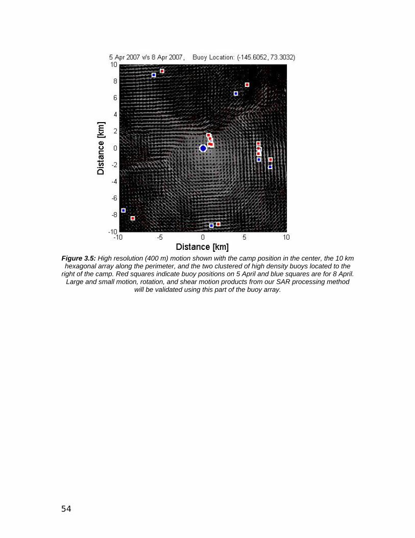
54

Figure 3.5: High resolution (400 m) motion shown with the camp position in the center, the 10 km hexagonal array along the perimeter, and the two clustered of high density buoys located to the

right of the camp. Red squares indicate buoy positions on 5 April and blue squares are for 8 April. Large and small motion, rotation, and shear motion products from our SAR processing method

will be validated using this part of the buoy array.

55

Figure 3.6: Zoomed in region showing the high density arrays of buoys.

3.6.2 Section summary This data set will be used to quality control and further validate the SAR motion tracking system developed at the University of Delaware Video/Image Modeling and Synthesis Laboratory. The range of scales tracked by the different types of buoys will be used as a quality control for differential motion types of shear, rotation, divergence, and large and small differential motion.

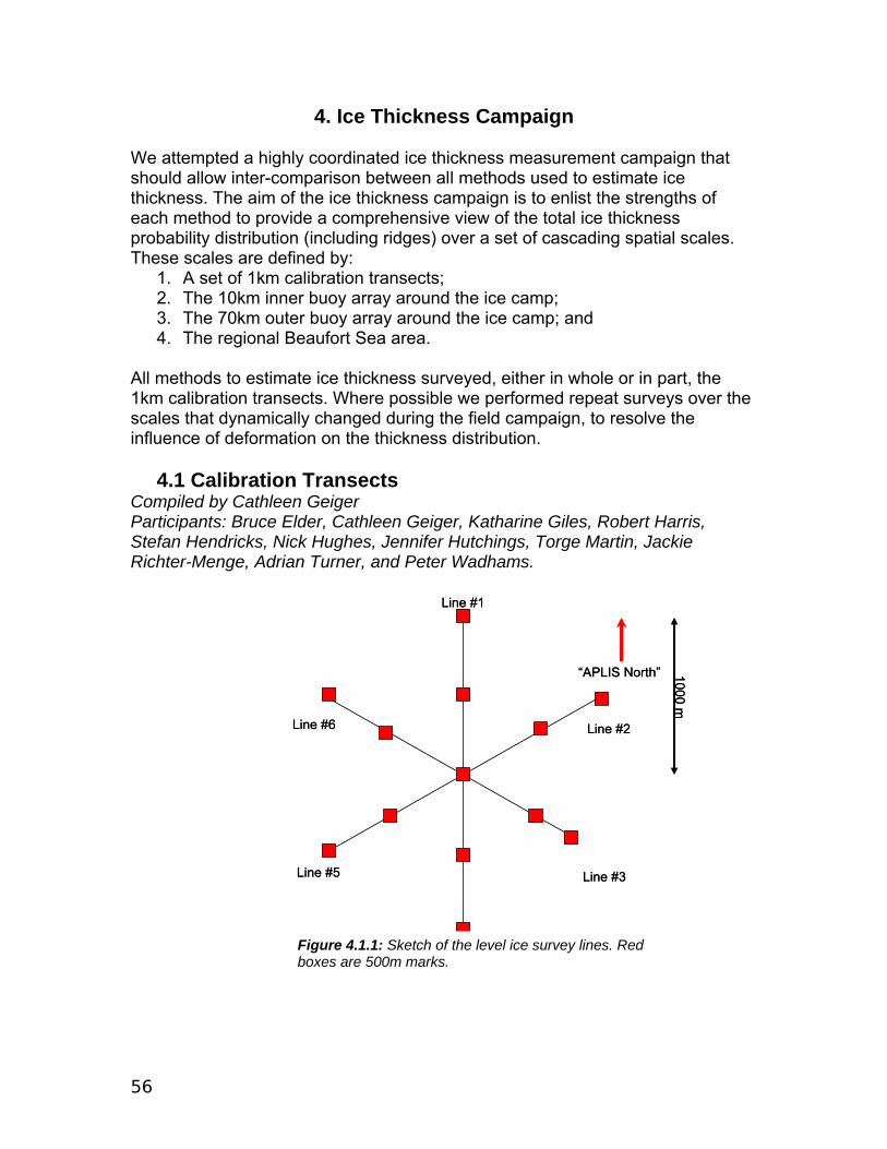
56

4. Ice Thickness Campaign We attempted a highly coordinated ice thickness measurement campaign that should allow inter-comparison between all methods used to estimate ice thickness. The aim of the ice thickness campaign is to enlist the strengths of each method to provide a comprehensive view of the total ice thickness probability distribution (including ridges) over a set of cascading spatial scales. These scales are defined by:

1. A set of 1km calibration transects; 2. The 10km inner buoy array around the ice camp; 3. The 70km outer buoy array around the ice camp; and 4. The regional Beaufort Sea area.

All methods to estimate ice thickness surveyed, either in whole or in part, the 1km calibration transects. Where possible we performed repeat surveys over the scales that dynamically changed during the field campaign, to resolve the influence of deformation on the thickness distribution.

4.1 Calibration Transects Compiled by Cathleen Geiger Participants: Bruce Elder, Cathleen Geiger, Katharine Giles, Robert Harris, Stefan Hendricks, Nick Hughes, Jennifer Hutchings, Torge Martin, Jackie Richter-Menge, Adrian Turner, and Peter Wadhams.

“APLIS North” 1000 m

Line #1

Line #2

Line #3

Line #4

Line #5

Line #6

“APLIS North” 1000 m

Line #1

Line #2

Line #3

Line #4

Line #5

Line #6

Figure 4.1.1: Sketch of the level ice survey lines. Red boxes are 500m marks.

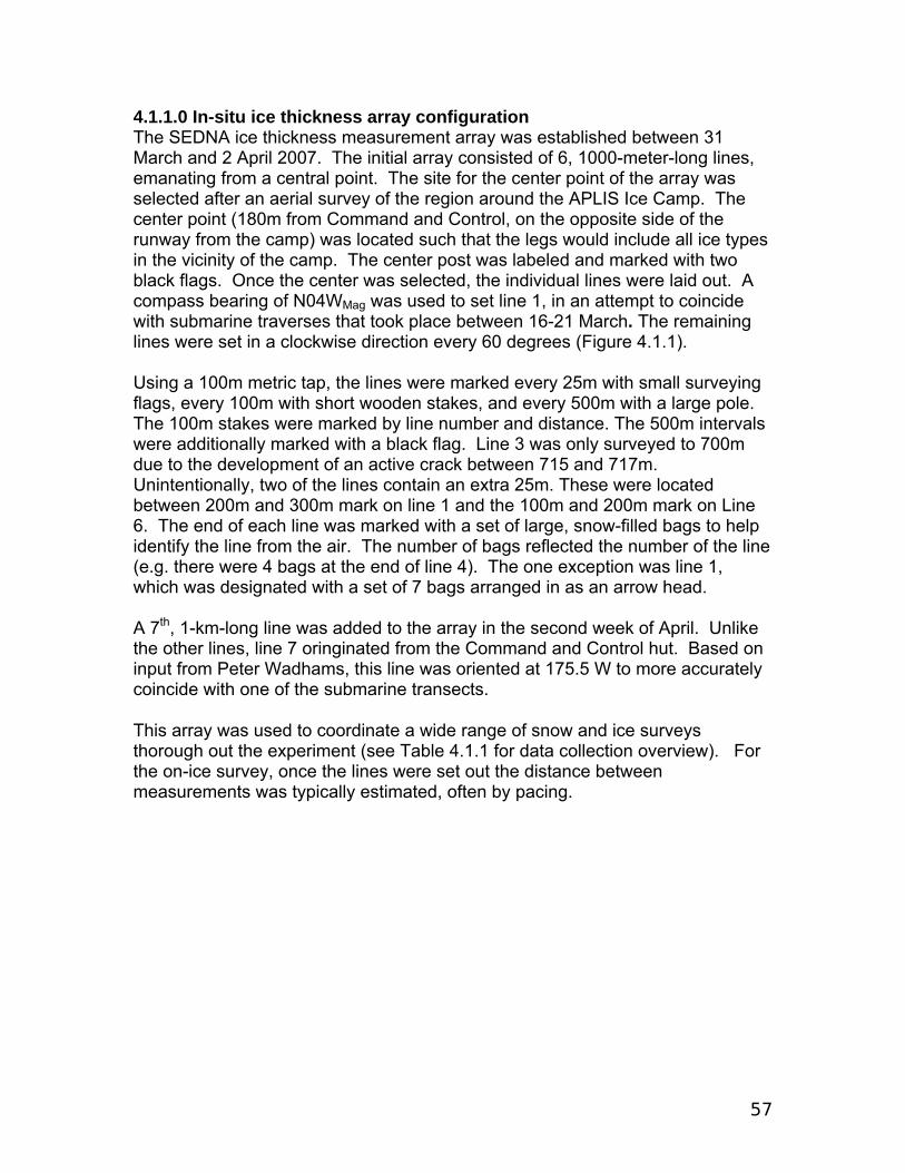
57

4.1.1.0 In-situ ice thickness array configuration The SEDNA ice thickness measurement array was established between 31 March and 2 April 2007. The initial array consisted of 6, 1000-meter-long lines, emanating from a central point. The site for the center point of the array was selected after an aerial survey of the region around the APLIS Ice Camp. The center point (180m from Command and Control, on the opposite side of the runway from the camp) was located such that the legs would include all ice types in the vicinity of the camp. The center post was labeled and marked with two black flags. Once the center was selected, the individual lines were laid out. A compass bearing of N04WMag was used to set line 1, in an attempt to coincide with submarine traverses that took place between 16-21 March. The remaining lines were set in a clockwise direction every 60 degrees (Figure 4.1.1). Using a 100m metric tap, the lines were marked every 25m with small surveying flags, every 100m with short wooden stakes, and every 500m with a large pole. The 100m stakes were marked by line number and distance. The 500m intervals were additionally marked with a black flag. Line 3 was only surveyed to 700m due to the development of an active crack between 715 and 717m. Unintentionally, two of the lines contain an extra 25m. These were located between 200m and 300m mark on line 1 and the 100m and 200m mark on Line 6. The end of each line was marked with a set of large, snow-filled bags to help identify the line from the air. The number of bags reflected the number of the line (e.g. there were 4 bags at the end of line 4). The one exception was line 1, which was designated with a set of 7 bags arranged in as an arrow head. A 7th, 1-km-long line was added to the array in the second week of April. Unlike the other lines, line 7 oringinated from the Command and Control hut. Based on input from Peter Wadhams, this line was oriented at 175.5 W to more accurately coincide with one of the submarine transects. This array was used to coordinate a wide range of snow and ice surveys thorough out the experiment (see Table 4.1.1 for data collection overview). For the on-ice survey, once the lines were set out the distance between measurements was typically estimated, often by pacing.

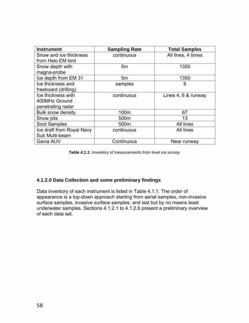
58

Instrument Sampling Rate Total Samples Snow and ice thickness from Helo EM bird

continuous All lines, 4 times

Snow depth with magna-probe

5m 1350

Ice depth from EM 31 5m 1350 Ice thickness and freeboard (drilling)

samples 9

Ice thickness with 400MHz Ground penetrating radar

continuous Lines 4, 6 & runway

Bulk snow density 100m 67 Snow pits 500m 13 Soot Samples 500m All lines Ice draft from Royal Navy Sub Multi-beam

continuous All lines

Gavia AUV Continuous Near runway

Table 4.1.1: Inventory of measurements from level ice survey. 4.1.2.0 Data Collection and some preliminary findings Data inventory of each instrument is listed in Table 4.1.1. The order of appearance is a top-down approach starting from aerial samples, non-invasive surface samples, invasive surface samples, and last but by no means least underwater samples. Sections 4.1.2.1 to 4.1.2.6 present a preliminary overview of each data set.

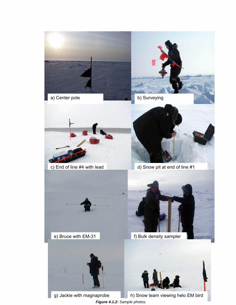
59

a) Center pole b) Surveying

c) End of line #4 with lead d) Snow pit at end of line #1

e) Bruce with EM-31 f) Bulk density sampler

g) Jackie with magnaprobe h) Snow team viewing helo EM bird Figure 4.1.2: Sample photos.

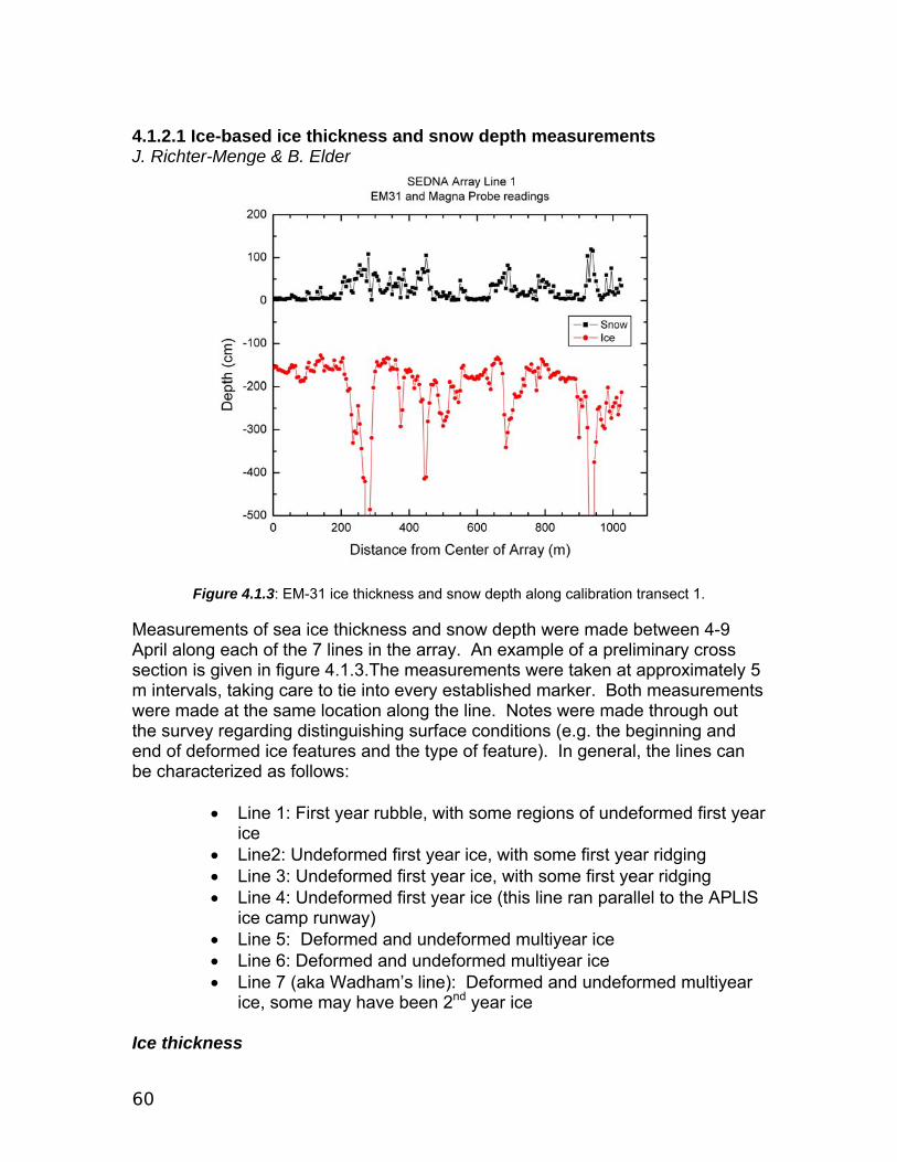
60

4.1.2.1 Ice-based ice thickness and snow depth measurements J. Richter-Menge & B. Elder

Figure 4.1.3: EM-31 ice thickness and snow depth along calibration transect 1.

Measurements of sea ice thickness and snow depth were made between 4-9 April along each of the 7 lines in the array. An example of a preliminary cross section is given in figure 4.1.3.The measurements were taken at approximately 5 m intervals, taking care to tie into every established marker. Both measurements were made at the same location along the line. Notes were made through out the survey regarding distinguishing surface conditions (e.g. the beginning and end of deformed ice features and the type of feature). In general, the lines can be characterized as follows:

• Line 1: First year rubble, with some regions of undeformed first year ice

• Line2: Undeformed first year ice, with some first year ridging • Line 3: Undeformed first year ice, with some first year ridging • Line 4: Undeformed first year ice (this line ran parallel to the APLIS

ice camp runway) • Line 5: Deformed and undeformed multiyear ice • Line 6: Deformed and undeformed multiyear ice • Line 7 (aka Wadham’s line): Deformed and undeformed multiyear

ice, some may have been 2nd year ice Ice thickness

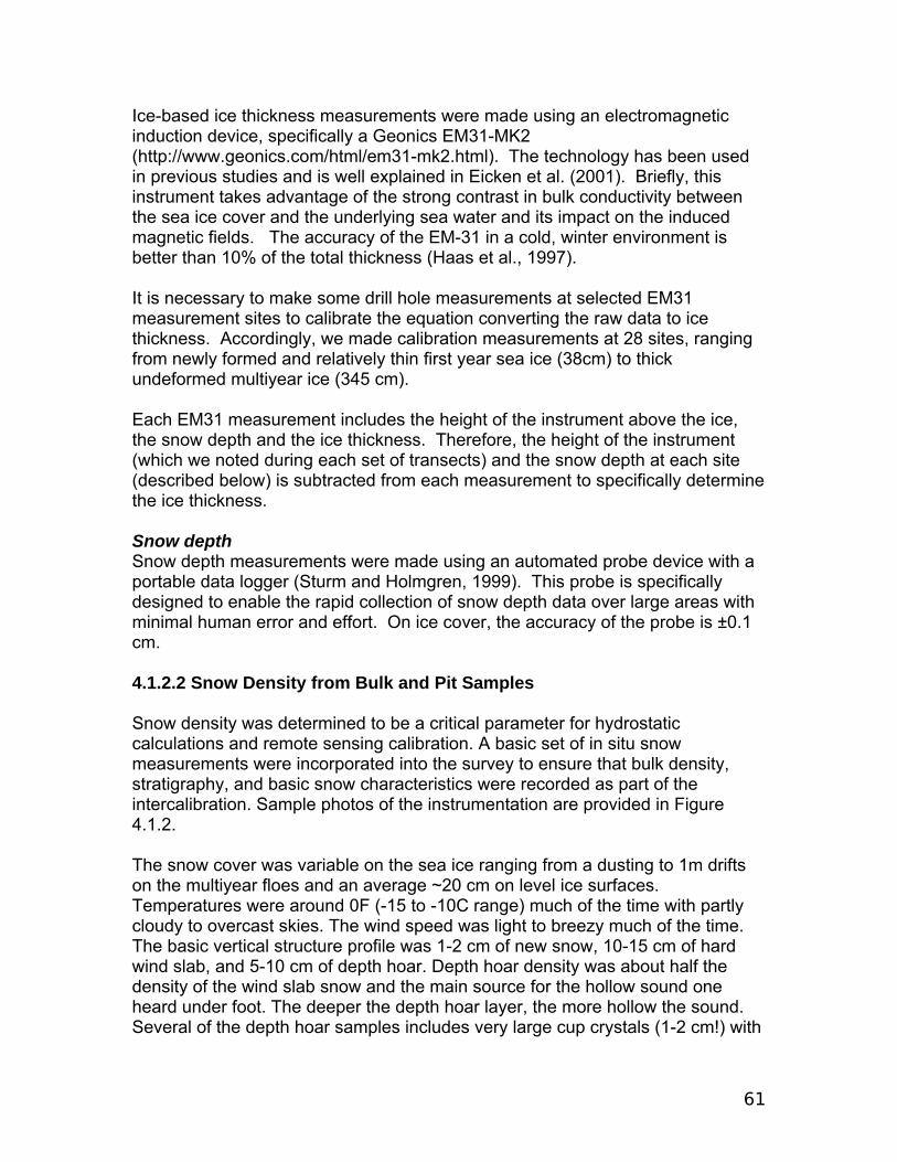
61

Ice-based ice thickness measurements were made using an electromagnetic induction device, specifically a Geonics EM31-MK2 (http://www.geonics.com/html/em31-mk2.html). The technology has been used in previous studies and is well explained in Eicken et al. (2001). Briefly, this instrument takes advantage of the strong contrast in bulk conductivity between the sea ice cover and the underlying sea water and its impact on the induced magnetic fields. The accuracy of the EM-31 in a cold, winter environment is better than 10% of the total thickness (Haas et al., 1997). It is necessary to make some drill hole measurements at selected EM31 measurement sites to calibrate the equation converting the raw data to ice thickness. Accordingly, we made calibration measurements at 28 sites, ranging from newly formed and relatively thin first year sea ice (38cm) to thick undeformed multiyear ice (345 cm). Each EM31 measurement includes the height of the instrument above the ice, the snow depth and the ice thickness. Therefore, the height of the instrument (which we noted during each set of transects) and the snow depth at each site (described below) is subtracted from each measurement to specifically determine the ice thickness.

Snow depth Snow depth measurements were made using an automated probe device with a portable data logger (Sturm and Holmgren, 1999). This probe is specifically designed to enable the rapid collection of snow depth data over large areas with minimal human error and effort. On ice cover, the accuracy of the probe is ±0.1 cm. 4.1.2.2 Snow Density from Bulk and Pit Samples Snow density was determined to be a critical parameter for hydrostatic calculations and remote sensing calibration. A basic set of in situ snow measurements were incorporated into the survey to ensure that bulk density, stratigraphy, and basic snow characteristics were recorded as part of the intercalibration. Sample photos of the instrumentation are provided in Figure 4.1.2. The snow cover was variable on the sea ice ranging from a dusting to 1m drifts on the multiyear floes and an average ~20 cm on level ice surfaces. Temperatures were around 0F (-15 to -10C range) much of the time with partly cloudy to overcast skies. The wind speed was light to breezy much of the time. The basic vertical structure profile was 1-2 cm of new snow, 10-15 cm of hard wind slab, and 5-10 cm of depth hoar. Depth hoar density was about half the density of the wind slab snow and the main source for the hollow sound one heard under foot. The deeper the depth hoar layer, the more hollow the sound. Several of the depth hoar samples includes very large cup crystals (1-2 cm!) with

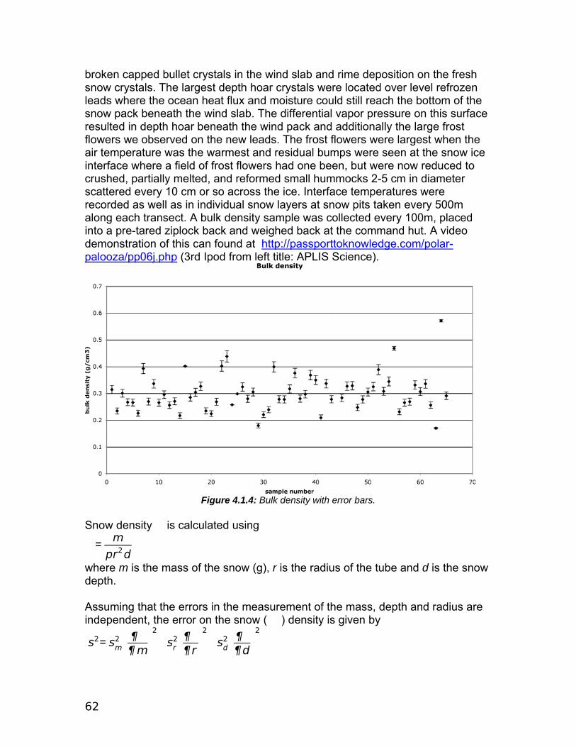
62

broken capped bullet crystals in the wind slab and rime deposition on the fresh snow crystals. The largest depth hoar crystals were located over level refrozen leads where the ocean heat flux and moisture could still reach the bottom of the snow pack beneath the wind slab. The differential vapor pressure on this surface resulted in depth hoar beneath the wind pack and additionally the large frost flowers we observed on the new leads. The frost flowers were largest when the air temperature was the warmest and residual bumps were seen at the snow ice interface where a field of frost flowers had one been, but were now reduced to crushed, partially melted, and reformed small hummocks 2-5 cm in diameter scattered every 10 cm or so across the ice. Interface temperatures were recorded as well as in individual snow layers at snow pits taken every 500m along each transect. A bulk density sample was collected every 100m, placed into a pre-tared ziplock back and weighed back at the command hut. A video demonstration of this can found at http://passporttoknowledge.com/polar-palooza/pp06j.php (3rd Ipod from left title: APLIS Science).

Figure 4.1.4: Bulk density with error bars.

Snow density � is calculated using

�= m

pr2d

where m is the mass of the snow (g), r is the radius of the tube and d is the snow depth. Assuming that the errors in the measurement of the mass, depth and radius are independent, the error on the snow (��) density is given by

s�2= sm

2 �¶�¶m�2�sr

2�¶�¶r�

2

�sd2�¶�

¶d�2

63

s�2= sm

2 �1pr2d�

2

�sr2�−2m

pr3d�2

�sd2�−m

pr2d2�2

where �m is the error in the measurement of the snow mass (± 0.5 g), �r is the error in the measurement of the tube radius (± 0.1 cm) and �d is the error in the measurement of the snow depth (± 1 cm). r equals 4.15 cm and d and m vary with each sample. Figure 4.1.4 shows the bulk snow density measurements with error bars for each measurement (± �s). These initial findings and associated uncertainties give us confidence that we were consistent in our data collection methods. 4.1.2.3 Soot Samples for Tom Grenfell and Steve Warren Soot samples were collected for Tom Grenfell and Steve Warren as part of the snow pit measurement effort. Samples were collected to a depth of 20 cm or the upper half whenever possible. When only a dusting of snow was available, the whole sample was used as this was usually fresh snow on multiyear. We followed a set of prescribed instructions set up by Tom Grenfell which included putting on a pair of food grade clean plastic gloves (2 pairs) over our glove liners; facing into the wind; collecting a clean snow sample with a clean sampling spoon; and marking the package. When we collected samples we were on foot pulling our sleds to minimize contamination. Sources of contamination for this type of sampling included the aircraft runway, generator hut, and helicopter. We tried to sample away from these except for two control sites on either side of the runway which we marked clearly for testing elevated contamination. We quality controlled our efforts through discussions and cross check with Bill Simson from the snow chemistry team to collect this data to the best ability given the team composition available on the ice. See appendix 3 for the list of samples collected. 4.1.2.4 Ground Penetrating RADAR A 400 MHz ground penetrating radar (GPR) antenna and recording unit from Geophysical Survey Systems, Inc (GSSI) was used to collect 100 KHz samples in continuous mode. The GPR was used to survey the six survey lines of the hexagonal array, the Wad1 survey line and the perimeter of Peter Wadhams 100 m square survey area, over which ice thickness, ice freeboard and snow depth measurements have been made every 10 meters. The radar antenna was pulled in a sledge along the ground while the control unit was carried along side. Each line was walked at a steady pace so that the time elapsed between marked points can be converted into a distance. Single markers were added to the data to indicate when the radar antenna passed a distance marker every 25 m (every 10 m for Peter Wadhams Survey area). Double check marks in the data indicate stopping and restarting walking during the survey (data with in the double stop – re-start check marks are ignored). Triple check marks indicate the start and end of each survey. After each line was surveyed, notes were taken describing the features along the line such as snowdrifts, ridges, missing marker flags, along with explanations of double check marks. Initial inspection of the data showed a

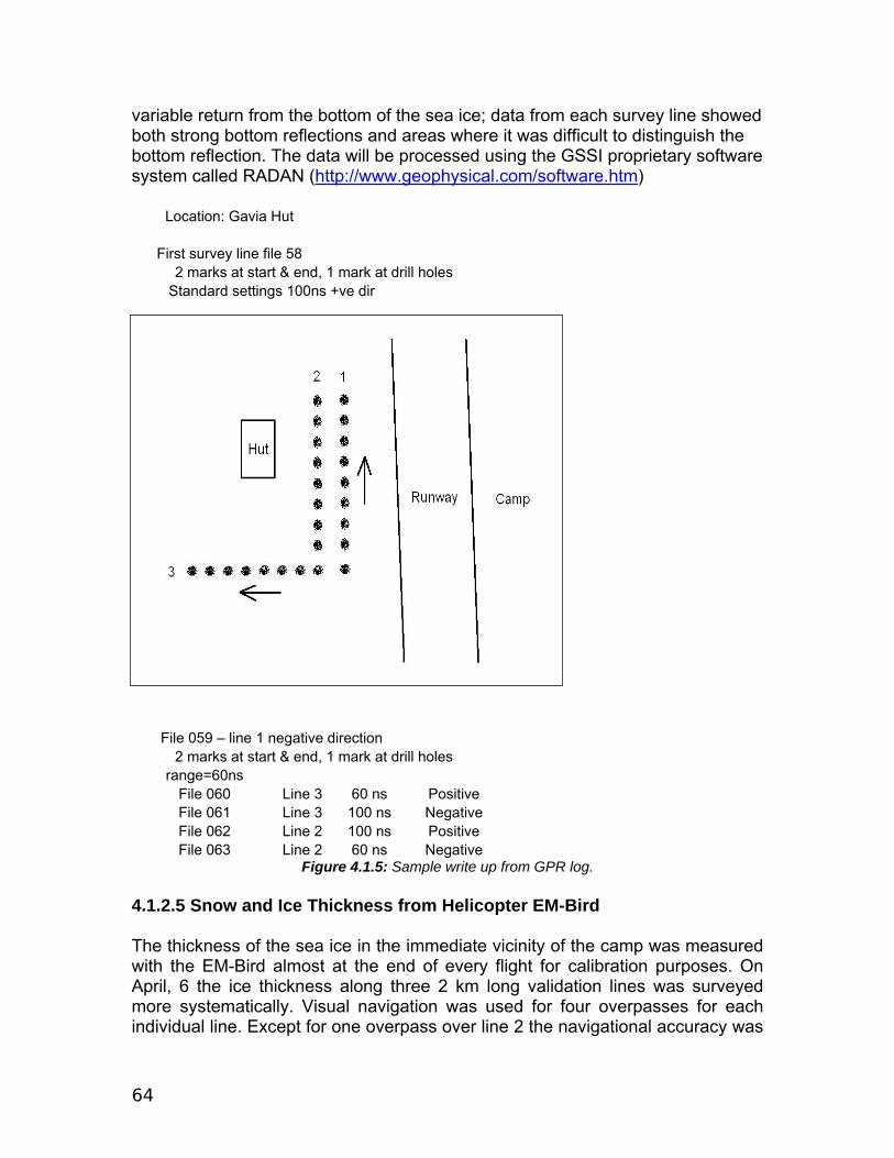
64

variable return from the bottom of the sea ice; data from each survey line showed both strong bottom reflections and areas where it was difficult to distinguish the bottom reflection. The data will be processed using the GSSI proprietary software system called RADAN (http://www.geophysical.com/software.htm)

Location: Gavia Hut

First survey line file 58 2 marks at start & end, 1 mark at drill holes

Standard settings 100ns +ve dir

File 059 – line 1 negative direction 2 marks at start & end, 1 mark at drill holes

range=60ns File 060 Line 3 60 ns Positive File 061 Line 3 100 ns Negative File 062 Line 2 100 ns Positive File 063 Line 2 60 ns Negative

Figure 4.1.5: Sample write up from GPR log. 4.1.2.5 Snow and Ice Thickness from Helicopter EM-Bird The thickness of the sea ice in the immediate vicinity of the camp was measured with the EM-Bird almost at the end of every flight for calibration purposes. On April, 6 the ice thickness along three 2 km long validation lines was surveyed more systematically. Visual navigation was used for four overpasses for each individual line. Except for one overpass over line 2 the navigational accuracy was

65

sufficient to align the EM-Bird data with in situ measurements (Figure 2.1.1). To compensate for sea ice drift the latitude/longitude positions are converted in a cartesian APLIS reference frame, which is defined by the GPS of the camp as origin and a northward pointing y-axis.

Figure 4.1.6: Sea ice thickness map for three validation lines close to the ice camp on April, 6

The thickness profiles of the individual lines are displayed in Figures 4.1.7-4.1.9. The black squares indicate the position where the operator has marked the beginning and end of the line manually in the data. These positions can deviate from each other since the position of the bird relative to the helicopter is not precisely known during the flight. Additionally, three transects southwest of the camp were flown to sample sea ice thickness on a data acquisition site of a submarine multi-beam sonar. These three transects have a spacing of approximately 50 m. The sea ice thickness distribution of the entire profile is displayed in Figure 4.1.10. The distribution is dominated by a modal thickness of 1.6-1.7 m, which is in good agreement with auger drill-hole measurements. The mean ice thickness amounts to 2.59 m (median: 2.30 m) with a standard deviation of 1.18 m. Line 1 includes two important features of the measurements. First, it mainly covers the runway next to the camp, which was built on pure level ice (see Figure 4.1.7, distances ca. 800–1100 m). At position 2050 m one can see the ridge site that has been in focus of extensive thickness measurements by drilling, diving, EM-Bird and AUV flying. Lines 2 and 3 show impressively the high

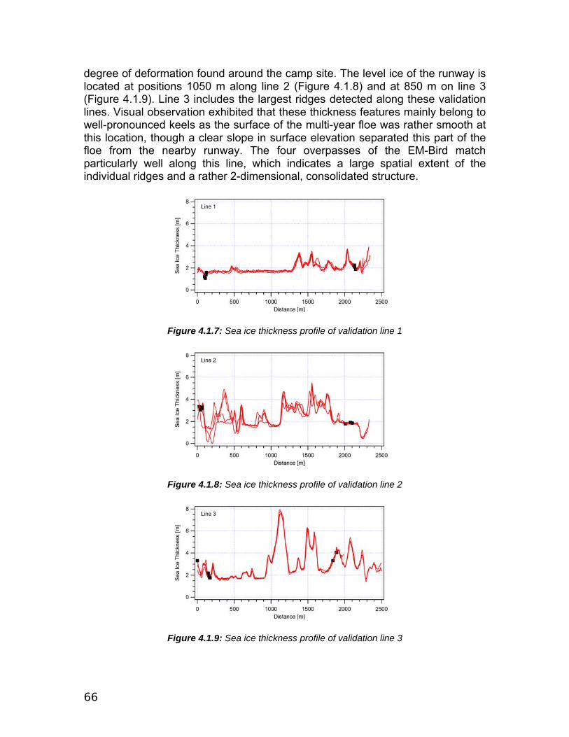
66

degree of deformation found around the camp site. The level ice of the runway is located at positions 1050 m along line 2 (Figure 4.1.8) and at 850 m on line 3 (Figure 4.1.9). Line 3 includes the largest ridges detected along these validation lines. Visual observation exhibited that these thickness features mainly belong to well-pronounced keels as the surface of the multi-year floe was rather smooth at this location, though a clear slope in surface elevation separated this part of the floe from the nearby runway. The four overpasses of the EM-Bird match particularly well along this line, which indicates a large spatial extent of the individual ridges and a rather 2-dimensional, consolidated structure.

Figure 4.1.7: Sea ice thickness profile of validation line 1

Figure 4.1.8: Sea ice thickness profile of validation line 2

Figure 4.1.9: Sea ice thickness profile of validation line 3

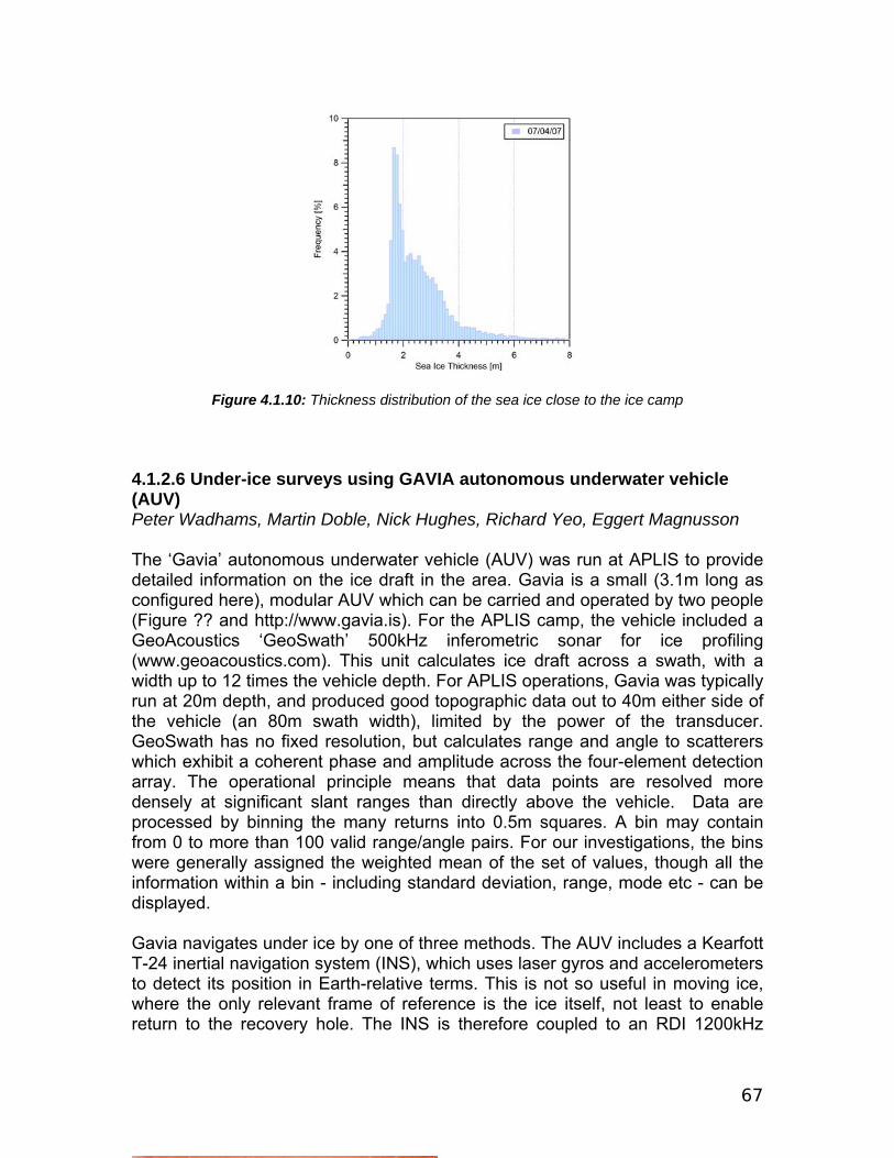
67

Figure 4.1.10: Thickness distribution of the sea ice close to the ice camp 4.1.2.6 Under-ice surveys using GAVIA autonomous underwater vehicle (AUV) Peter Wadhams, Martin Doble, Nick Hughes, Richard Yeo, Eggert Magnusson The ‘Gavia’ autonomous underwater vehicle (AUV) was run at APLIS to provide detailed information on the ice draft in the area. Gavia is a small (3.1m long as configured here), modular AUV which can be carried and operated by two people (Figure ?? and http://www.gavia.is). For the APLIS camp, the vehicle included a GeoAcoustics ‘GeoSwath’ 500kHz inferometric sonar for ice profiling (www.geoacoustics.com). This unit calculates ice draft across a swath, with a width up to 12 times the vehicle depth. For APLIS operations, Gavia was typically run at 20m depth, and produced good topographic data out to 40m either side of the vehicle (an 80m swath width), limited by the power of the transducer. GeoSwath has no fixed resolution, but calculates range and angle to scatterers which exhibit a coherent phase and amplitude across the four-element detection array. The operational principle means that data points are resolved more densely at significant slant ranges than directly above the vehicle. Data are processed by binning the many returns into 0.5m squares. A bin may contain from 0 to more than 100 valid range/angle pairs. For our investigations, the bins were generally assigned the weighted mean of the set of values, though all the information within a bin - including standard deviation, range, mode etc - can be displayed. Gavia navigates under ice by one of three methods. The AUV includes a Kearfott T-24 inertial navigation system (INS), which uses laser gyros and accelerometers to detect its position in Earth-relative terms. This is not so useful in moving ice, where the only relevant frame of reference is the ice itself, not least to enable return to the recovery hole. The INS is therefore coupled to an RDI 1200kHz

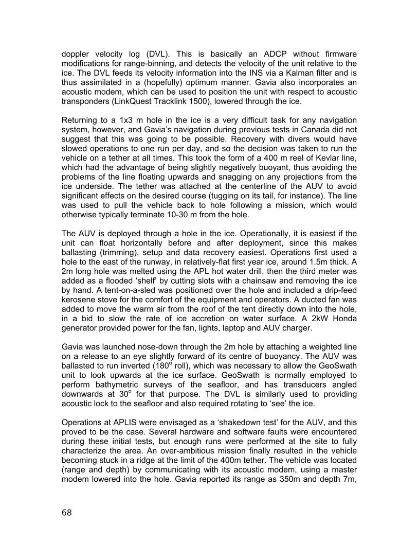
68

doppler velocity log (DVL). This is basically an ADCP without firmware modifications for range-binning, and detects the velocity of the unit relative to the ice. The DVL feeds its velocity information into the INS via a Kalman filter and is thus assimilated in a (hopefully) optimum manner. Gavia also incorporates an acoustic modem, which can be used to position the unit with respect to acoustic transponders (LinkQuest Tracklink 1500), lowered through the ice. Returning to a 1x3 m hole in the ice is a very difficult task for any navigation system, however, and Gavia’s navigation during previous tests in Canada did not suggest that this was going to be possible. Recovery with divers would have slowed operations to one run per day, and so the decision was taken to run the vehicle on a tether at all times. This took the form of a 400 m reel of Kevlar line, which had the advantage of being slightly negatively buoyant, thus avoiding the problems of the line floating upwards and snagging on any projections from the ice underside. The tether was attached at the centerline of the AUV to avoid significant effects on the desired course (tugging on its tail, for instance). The line was used to pull the vehicle back to hole following a mission, which would otherwise typically terminate 10-30 m from the hole. The AUV is deployed through a hole in the ice. Operationally, it is easiest if the unit can float horizontally before and after deployment, since this makes ballasting (trimming), setup and data recovery easiest. Operations first used a hole to the east of the runway, in relatively-flat first year ice, around 1.5m thick. A 2m long hole was melted using the APL hot water drill, then the third meter was added as a flooded ‘shelf’ by cutting slots with a chainsaw and removing the ice by hand. A tent-on-a-sled was positioned over the hole and included a drip-feed kerosene stove for the comfort of the equipment and operators. A ducted fan was added to move the warm air from the roof of the tent directly down into the hole, in a bid to slow the rate of ice accretion on water surface. A 2kW Honda generator provided power for the fan, lights, laptop and AUV charger. Gavia was launched nose-down through the 2m hole by attaching a weighted line on a release to an eye slightly forward of its centre of buoyancy. The AUV was ballasted to run inverted (180o roll), which was necessary to allow the GeoSwath unit to look upwards at the ice surface. GeoSwath is normally employed to perform bathymetric surveys of the seafloor, and has transducers angled downwards at 30o for that purpose. The DVL is similarly used to providing acoustic lock to the seafloor and also required rotating to ‘see’ the ice. Operations at APLIS were envisaged as a ‘shakedown test’ for the AUV, and this proved to be the case. Several hardware and software faults were encountered during these initial tests, but enough runs were performed at the site to fully characterize the area. An over-ambitious mission finally resulted in the vehicle becoming stuck in a ridge at the limit of the 400m tether. The vehicle was located (range and depth) by communicating with its acoustic modem, using a master modem lowered into the hole. Gavia reported its range as 350m and depth 7m,

69

with 21o of pitch (nose down). Range and bearing were confirmed using a Datasonics LXT transponder, loaned by APL. Attempts to free the vehicle by commanding the propellor over the modem link proved unsuccessful. A further 300m of line was therefore added to the spool and a 2.5kg lead weight fixed to the mid-point of the lines, in a bid to pull the vehicle downwards out of the ridge and allow it to be pulled back on the line. This was initially unsuccessful, but pulling the weight back to the hole – to add more weight – freed the vehicle and it was pulled back to the hole without further drama. The ice drafts calculated by the GeoSwath were validated by a dense grid of holes drilled in a 100x100m grid around the hole, at 10m spacing (Figure 4.1.11). It can be seen from the drilling results that the ice consisted of generally undeformed first-year ice, nowhere exceeding 2 m in draft, with a typical draft of 1.3 – 1.6 m but with occasional point defects (small pointed pinnacles, probably formed from minor deformations when the ice was young) extending to 1.9 m. Of necessity this picture is a smeared-out one because of the 10 m hole spacing, but it does bear a remarkable resemblance to the picture generated by the Geoswath (see also photograph Figure 4.1.12) which likewise shows drafts in the 1-2 m range and point defects rather than linear ridges.

Figure 4.1.11: Contour map of ice drafts near first AUV site, from holes drilled in 10 m grid. Drafts in cm.

“North” on grid is 015º True.

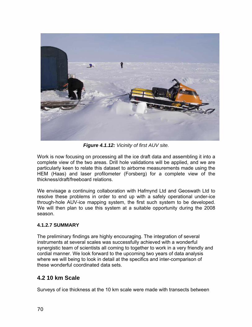
70

Figure 4.1.12: Vicinity of first AUV site. Work is now focusing on processing all the ice draft data and assembling it into a complete view of the two areas. Drill hole validations will be applied, and we are particularly keen to relate this dataset to airborne measurements made using the HEM (Haas) and laser profilometer (Forsberg) for a complete view of the thickness/draft/freeboard relations. We envisage a continuing collaboration with Hafmynd Ltd and Geoswath Ltd to resolve these problems in order to end up with a safely operational under-ice through-hole AUV-ice mapping system, the first such system to be developed. We will then plan to use this system at a suitable opportunity during the 2008 season. 4.1.2.7 SUMMARY The preliminary findings are highly encouraging. The integration of several instruments at several scales was successfully achieved with a wonderful synergistic team of scientists all coming to together to work in a very friendly and cordial manner. We look forward to the upcoming two years of data analysis where we will being to look in detail at the specifics and inter-comparison of these wonderful coordinated data sets. 4.2 10 km Scale Surveys of ice thickness at the 10 km scale were made with transects between

71

buoys in the inner buoy array. We ensured that the most recent position of buoys, emailed to the ice camp at 7am every morning, was used to calculate Helicopter flight tracks. This worked very well for the 10km surveys, where buoys were located visually at the end of all flight lines taken on April 9th. It was not so simple to align the submarine tracks with buoy position, as the submarine surveys were performed before the start of the NSF science camp. We aligned submarine tracks to the APL sonar range. This range was aligned 5.5 degrees to the west of true north during the surveys. Due to this 5 degree mismatch between buoy deployment location and the sonar range, submarine and helicopter tracks do not exactly match. As we can not ensure the same ice was sampled close to the camp with both, we will need to rely on statistical comparisons between the two methods.

4.2.1 Data collection plans for the US Alexandria Plans for a submarine survey of the 10km region around the ice camp were provided by Jennifer Hutchings to Jeff Gosset, Arctic Submarine Laboratory. These plans where drawn up from discussions between Dr. Hutchings, Mark Wednesham (Applied Physics Laboratory) and Peter Wadhams. There were two scenarios considered: either 6 hours or 20 hours of cruising time.

Figure 4.2.1: Proposed tracks for submarine

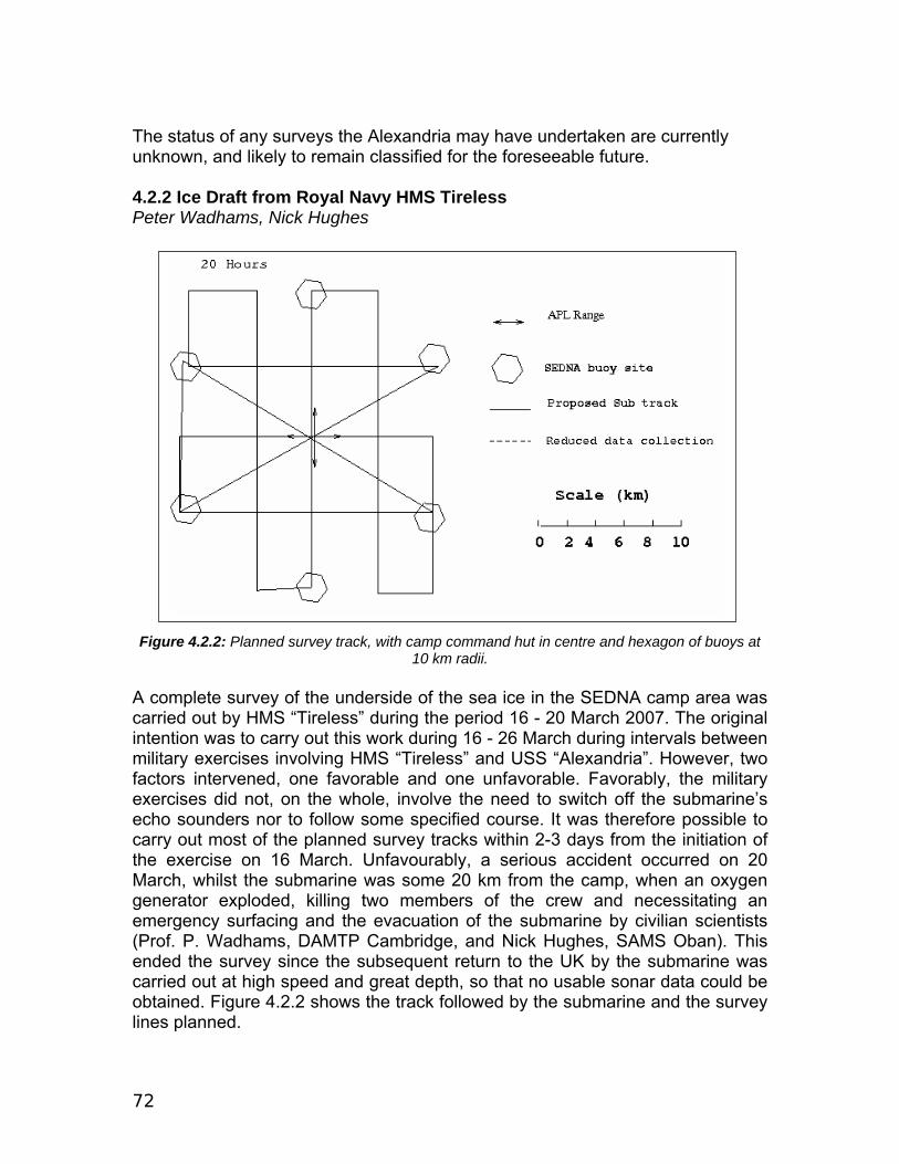
72

The status of any surveys the Alexandria may have undertaken are currently unknown, and likely to remain classified for the foreseeable future. 4.2.2 Ice Draft from Royal Navy HMS Tireless Peter Wadhams, Nick Hughes

Figure 4.2.2: Planned survey track, with camp command hut in centre and hexagon of buoys at

10 km radii. A complete survey of the underside of the sea ice in the SEDNA camp area was carried out by HMS “Tireless” during the period 16 - 20 March 2007. The original intention was to carry out this work during 16 - 26 March during intervals between military exercises involving HMS “Tireless” and USS “Alexandria”. However, two factors intervened, one favorable and one unfavorable. Favorably, the military exercises did not, on the whole, involve the need to switch off the submarine’s echo sounders nor to follow some specified course. It was therefore possible to carry out most of the planned survey tracks within 2-3 days from the initiation of the exercise on 16 March. Unfavourably, a serious accident occurred on 20 March, whilst the submarine was some 20 km from the camp, when an oxygen generator exploded, killing two members of the crew and necessitating an emergency surfacing and the evacuation of the submarine by civilian scientists (Prof. P. Wadhams, DAMTP Cambridge, and Nick Hughes, SAMS Oban). This ended the survey since the subsequent return to the UK by the submarine was carried out at high speed and great depth, so that no usable sonar data could be obtained. Figure 4.2.2 shows the track followed by the submarine and the survey lines planned.

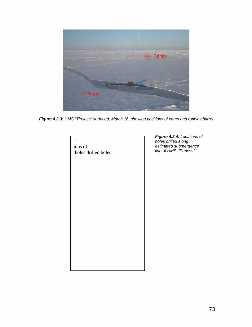
73

Figure 4.2.3: HMS “Tireless” surfaced, March 16, showing positions of camp and runway barrel

� ions of holes drilled holes

Figure 4.2.4: Locations of holes drilled along estimated submergence line of HMS “Tireless”.

74

The submarine was equipped with the following sonar systems:- • A Kongsberg Simrad EM3002 multibeam sonar operating at 300 kHz,

generating a 3-D digital terrain map of the ice underside, of swath width typically 100-120 m. This had already begun to malfunction before reaching the ice camp, due to water leakage into the sonar head and subsequently through the main cable connecting this to the interior of the submarine.

• An Admiralty 2077-pattern integrated sonar system, comprising an upward-looking sonar recording digitally, a sidescan sonar and a forward-looking “iceberg detector” sonar. The upward-looking sonar had begun to malfunction, but the sidescan sonar was operational throughout the survey and produced a continuous digital record to a range of 300 m either side of the submarine track, which is of great value for locating the submarine track on overall grids and ice maps of the area. The iceberg detector did not generate data of general scientific value.

• An Admiralty 780-pattern upward looking sonar of approximately 3º beamwidth recording on electrically sensitive paper at 48 kHz. This is a “traditional” system used on many previous submarine voyages back to 1976. It operated well throughout the survey and is the main source of quantitative ice thickness data.

Because of its water leakage the EM3002 system did not work during the survey, except for a few minutes of data which were obtained when the submarine submerged after spending 6 hours on the surface on 16 March 2007 near the ice camp, which presumably allowed the cable to temporarily dry out. As this record was especially valuable, an effort was made to reconstruct the boat’s track and to measure ice thickness at the surface along the first 1 km or so after the boat submerged. Data are still being analyzed and will be released as soon as possible. The analysis routine for 780 data, which is labor-intensive, involves:-

• digitization of envelope of sonar record using scanner with installed 780 software;

• removal of boat depth variations and porpoising by connecting open water stretches and generating, and subtracting, smooth curve;

• correction for boat speed variations using SNAPS (Ship’s Navigation and Positioning System) tapes;

• Generation of corrected draft-distance record and production of statistics from individual legs of survey, as per chapter 5 of “Ice in the Ocean” (P. Wadhams: Taylor and Francis, 2000).

This analysis is being carried out under ONR grant N00014-07-1-0517 to DAMTP, Cambridge.

75

4.2.3 Airborne laser scanner survey around the APLIS07 icecamp H. Skourup and R. Forsberg, Danish National Space Center, hsk@space.dtu.dk, rf@space.dtu.dk In connection with DAMOCLES field work 2007 the Danish National Space Center (DNSC) contributed with an extensive airborne survey in the area around APLIS07 ice camp on April 12, 2007. The main task was to collect high resolution laser scanner data in order to estimate the sea ice freeboard. The DNSC laser scanner system provides ice height data at a resolution of approx. 1 m in a 250 m wide swath. The flight tracks were chosen to be coincident to other ongoing sea ice activities in order to compare the results, giving deeper insight into various measurement methods and sea ice processes. In Figure 4.2.5 (left) all the flight tracks are mapped. An approximate 100 km long track was flown parallel to an ICESat track, and an approximate 70 km long line was flown coincident to earlier flown AWI helicopter borne EM-bird thickness measurements. The GPS ice drift information available at the flight epoch was used for waypoint definition. The small red inner box is shown in details in upper right corner of Fig. 1. It shows the flight tracks of a detailed mow-the-lawn pattern to survey the ice floe at which the ice camp was located and the adjacent runway area. An area of approx. 5 x 2 km was covered, centered on the APLIS camp. The spacing between the lines were narrower than the width of the laser scanner, and thus the entire area should be fully covered. Finally the large red outer box, shown in details in the lower right figure, maps the survey pattern corresponding to track lines (1-6) surveyed by a British nuclear submarine, which maps the sea ice from below by upward looking sonar (ULS). The return flight line no. 7 represents a survey line measured by EM. The laser scanner data from the survey has not yet been processed. The final product will be delivered as freeboard maps with a horizontal resolution ~1x1m. For an example see Figure 4.2.6. The width of the laser scanner is approximately the same as the flight altitude (~250 m), and the vertical precision are primarily determined by the errors of the GPS solutions in the order of decimeters, due to the long baselines. There is in total 3 scanner files (each ~200 Mb) each representing 1hr of data, and also scanner data flying into camp from Inuvik, Canada, on April 12, and leaving for Sachs Harbour, Canada, on April 13.

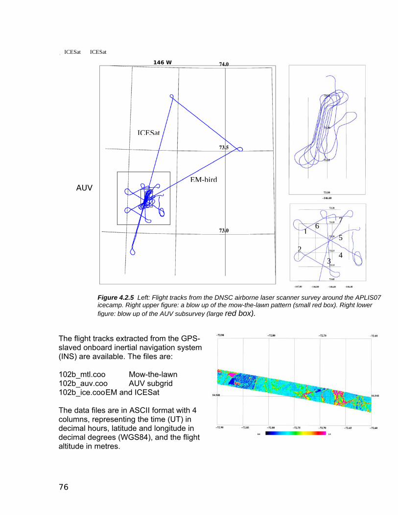
76

1 ICESat ICESat

The flight tracks extracted from the GPS-slaved onboard inertial navigation system (INS) are available. The files are: 102b_mtl.coo Mow-the-lawn 102b_auv.coo AUV subgrid 102b_ice.coo EM and ICESat The data files are in ASCII format with 4 columns, representing the time (UT) in decimal hours, latitude and longitude in decimal degrees (WGS84), and the flight altitude in metres.

AUV

Figure 4.2.5 Left: Flight tracks from the DNSC airborne laser scanner survey around the APLIS07 icecamp. Right upper figure: a blow up of the mow-the-lawn pattern (small red box). Right lower figure: blow up of the AUV subsurvey (large red box).

ICESat

EM-bird

1

23

4

5 6

7

146 W

77

4.2.3 Helicopter EM-bird Surveys Steffan Hendriks & Torge Martin Sea ice thickness within the inner buoy array was measured with the EM-Bird on two days: April, 5 (Figure 4.2.7) and April, 9 (Figure 4.2.8). The flight profile is characterized by three successive triangles with a side length of 10 km. The waypoints were calculated by buoy positions of the respective morning then using the current position of the ice camp to estimate the recent buoy positions at take-off time. On April, 9, the second flight, all buoys were spotted by the crew during the flight.

Figure 4.2.7 : Sea ice thickness map of the inner buoy array on April, 5

An example of how ice thickness has changed along the inner buoy array is displayed in Figure 4.2.9. Despite the fact that not exactly the same ice was profiled during the two flights the typical characteristics of the region, such as large leads and ridges, first and multi-year ice, known from the first flight were observed again in the second profile. This can also be seen from the mean and standard deviations given in Table 4.2.1 and the frequency distributions of ice thickness in Figure 4.2.10 (left). The change of the ice thickness distribution is displayed in Figure 4.2.10. A bin width of 10 cm is chosen for both histograms. The differences in ice thickness between the two profiles amount to less than 2 % for all bins. This confirms that the calibration of the EM-Bird was stable during both flights. The comparison of

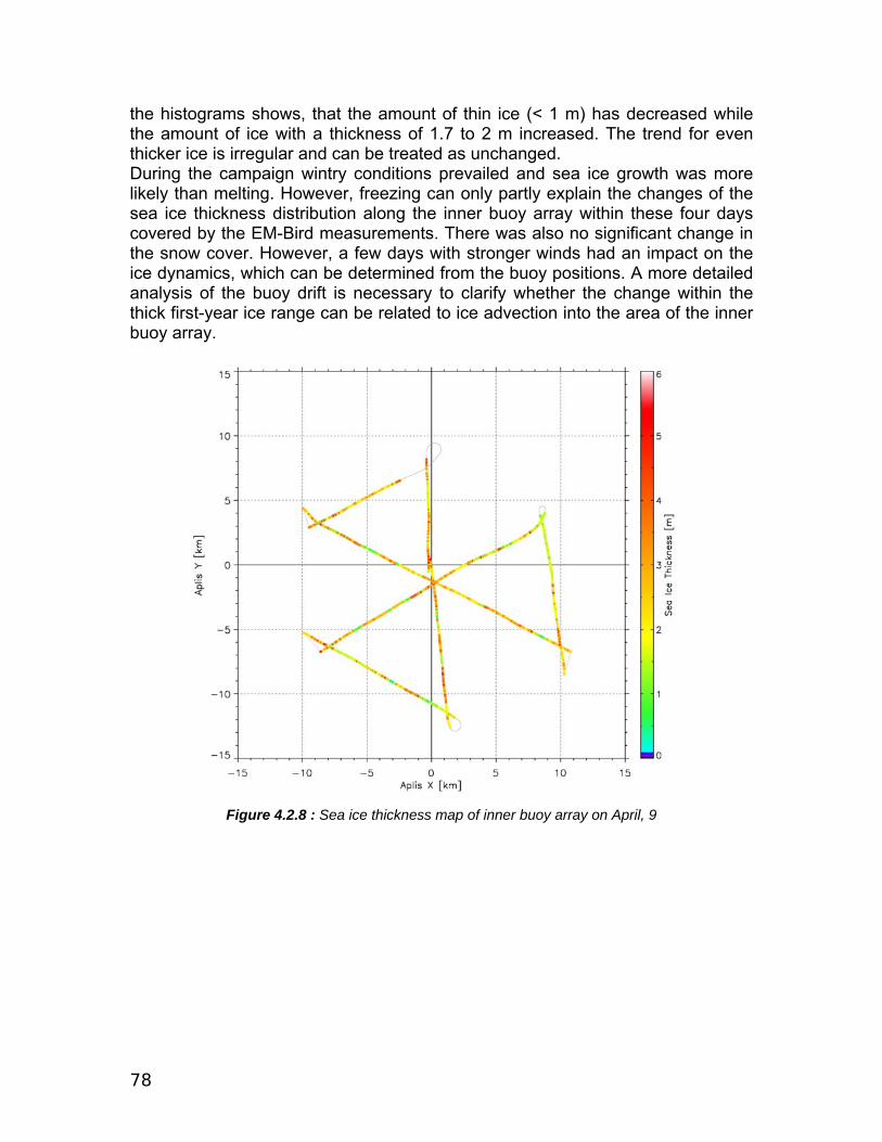
78

the histograms shows, that the amount of thin ice (< 1 m) has decreased while the amount of ice with a thickness of 1.7 to 2 m increased. The trend for even thicker ice is irregular and can be treated as unchanged. During the campaign wintry conditions prevailed and sea ice growth was more likely than melting. However, freezing can only partly explain the changes of the sea ice thickness distribution along the inner buoy array within these four days covered by the EM-Bird measurements. There was also no significant change in the snow cover. However, a few days with stronger winds had an impact on the ice dynamics, which can be determined from the buoy positions. A more detailed analysis of the buoy drift is necessary to clarify whether the change within the thick first-year ice range can be related to ice advection into the area of the inner buoy array.

Figure 4.2.8 : Sea ice thickness map of inner buoy array on April, 9

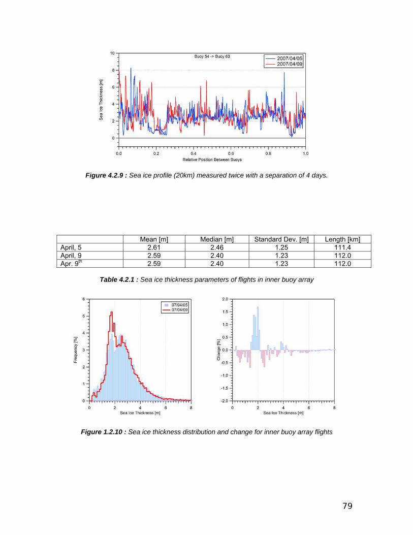
79

Figure 4.2.9 : Sea ice profile (20km) measured twice with a separation of 4 days. Mean [m] Median [m] Standard Dev. [m] Length [km] April, 5 2.61 2.46 1.25 111.4 April, 9 2.59 2.40 1.23 112.0 Apr. 9th 2.59 2.40 1.23 112.0

Table 4.2.1 : Sea ice thickness parameters of flights in inner buoy array

Figure 1.2.10 : Sea ice thickness distribution and change for inner buoy array flights

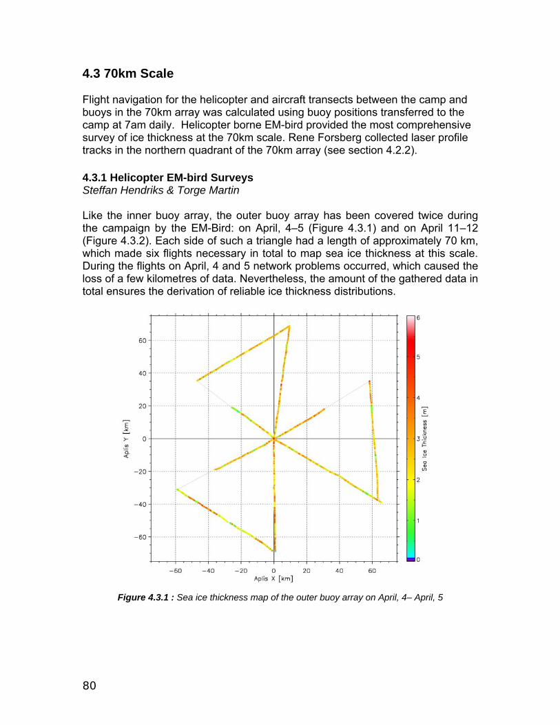
80

4.3 70km Scale Flight navigation for the helicopter and aircraft transects between the camp and buoys in the 70km array was calculated using buoy positions transferred to the camp at 7am daily. Helicopter borne EM-bird provided the most comprehensive survey of ice thickness at the 70km scale. Rene Forsberg collected laser profile tracks in the northern quadrant of the 70km array (see section 4.2.2). 4.3.1 Helicopter EM-bird Surveys Steffan Hendriks & Torge Martin Like the inner buoy array, the outer buoy array has been covered twice during the campaign by the EM-Bird: on April, 4–5 (Figure 4.3.1) and on April 11–12 (Figure 4.3.2). Each side of such a triangle had a length of approximately 70 km, which made six flights necessary in total to map sea ice thickness at this scale. During the flights on April, 4 and 5 network problems occurred, which caused the loss of a few kilometres of data. Nevertheless, the amount of the gathered data in total ensures the derivation of reliable ice thickness distributions.

Figure 4.3.1 : Sea ice thickness map of the outer buoy array on April, 4– April, 5

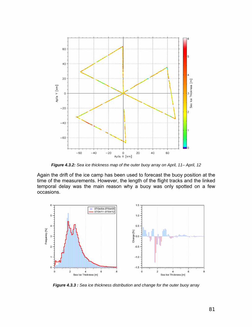
81

Figure 4.3.2: Sea ice thickness map of the outer buoy array on April, 11– April, 12

Again the drift of the ice camp has been used to forecast the buoy position at the time of the measurements. However, the length of the flight tracks and the linked temporal delay was the main reason why a buoy was only spotted on a few occasions.

Figure 4.3.3 : Sea ice thickness distribution and change for the outer buoy array

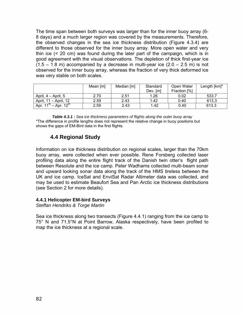
82

The time span between both surveys was larger than for the inner buoy array (6-8 days) and a much larger region was covered by the measurements. Therefore, the observed changes in the sea ice thickness distribution (Figure 4.3.4) are different to those observed for the inner buoy array. More open water and very thin ice (< 20 cm) was found during the later part of the campaign, which is in good agreement with the visual observations. The depletion of thick first-year ice (1.5 – 1.8 m) accompanied by a decrease in multi-year ice (2.0 – 2.5 m) is not observed for the inner buoy array, whereas the fraction of very thick deformed ice was very stable on both scales. Mean [m] Median [m] Standard

Dev. [m] Open Water Fraction [%]

Length [km]*

April, 4 – April, 5 2.70 2.51 1.26 0.02 533.7 April, 11 – April, 12 2.59 2.43 1.42 0.40 613.3 Apr. 11th – Apr. 12th 2.59 2.43 1.42 0.40 613.3

Table 4.3.1 : Sea ice thickness parameters of flights along the outer buoy array *The difference in profile lengths does not represent the relative change in buoy positions but shows the gaps of EM-Bird data in the first flights. 4.4 Regional Study Information on ice thickness distribution on regional scales, larger than the 70km buoy array, were collected when ever possible. Rene Forsberg collected laser profiling data along the entire flight track of the Danish twin otter’s flight path between Resolute and the ice camp. Peter Wadhams collected multi-beam sonar and upward looking sonar data along the track of the HMS tireless between the UK and ice camp. IceSat and EnviSat Radar Altimeter data was collected, and may be used to estimate Beaufort Sea and Pan Arctic ice thickness distributions (see Section 2 for more details). 4.4.1 Helicopter EM-bird Surveys Steffan Hendriks & Torge Martin Sea ice thickness along two transects (Figure 4.4.1) ranging from the ice camp to 75° N and 71.5°N at Point Barrow, Alaska respectively, have been profiled to map the ice thickness at a regional scale.

83

Figure 4.4.1 : Sea ice thickness map of two transects ranging from 75°N to 71.5°N on April, 10

and April, 13 The dataset can roughly be divided into two parts: one north (April, 10) and one south (April, 13) of the camp site. The flight to the north was a two-way profile, while the transect to Barrow was planed to transfer personnel and equipment from the camp to shore and additionally used for measurements. A quick look on the two profiles and the respective frequency distributions (Figure 4.4.2) exhibits a few distinct differences. While the modal thickness of the first-year ice is basically the same (two modes at 1.1 and 1.7 m), more open water and thick deformed ice (> 3 m) is present in the sea ice close to the coast. These differences between the two profiles can be explained by the large-scale motion of the Arctic sea ice cover, which forms a huge shear zone parallel to the Alaskan coastline. This enhances dynamic processes such as open water formation and deformation in this region. The ice camp was located in a region where the near-coast first-year ice cover changed into multi-year ice, where the latter has stronger resistive forces against deformation.

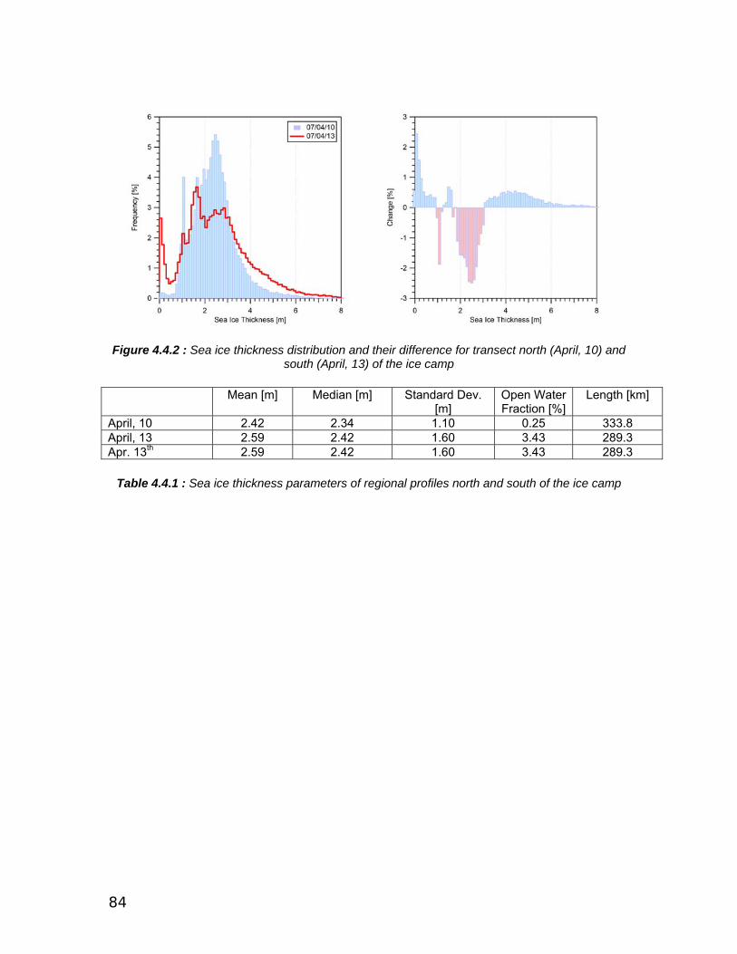
84

Figure 4.4.2 : Sea ice thickness distribution and their difference for transect north (April, 10) and south (April, 13) of the ice camp

Mean [m] Median [m] Standard Dev.

[m] Open Water Fraction [%]

Length [km]

April, 10 2.42 2.34 1.10 0.25 333.8 April, 13 2.59 2.42 1.60 3.43 289.3 Apr. 13th 2.59 2.42 1.60 3.43 289.3

Table 4.4.1 : Sea ice thickness parameters of regional profiles north and south of the ice camp

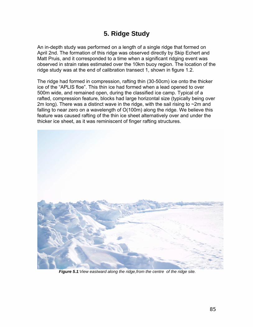
85

5. Ridge Study An in-depth study was performed on a length of a single ridge that formed on April 2nd. The formation of this ridge was observed directly by Skip Echert and Matt Pruis, and it corresponded to a time when a significant ridging event was observed in strain rates estimated over the 10km buoy region. The location of the ridge study was at the end of calibration transect 1, shown in figure 1.2. The ridge had formed in compression, rafting thin (30-50cm) ice onto the thicker ice of the “APLIS floe”. This thin ice had formed when a lead opened to over 500m wide, and remained open, during the classified ice camp. Typical of a rafted, compression feature, blocks had large horizontal size (typically being over 2m long). There was a distinct wave in the ridge, with the sail rising to ~2m and falling to near zero on a wavelength of O(100m) along the ridge. We believe this feature was caused rafting of the thin ice sheet alternatively over and under the thicker ice sheet, as it was reminiscent of finger rafting structures.

Figure 5.1:View eastward along the ridge,from the centre of the ridge site.

86

Figure 5.2: [top] Ridge crossing transect r6. [bottom] Ridge crossing transect r3. The red/yellow/block post was painted in 10cm segments.

Figure 5.3: Pat McKeown (6’1”) under the ridge. Photo by Mitch Osborne.

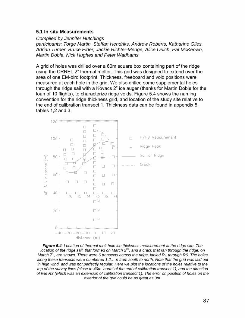
87

5.1 In-situ Measurements Compiled by Jennifer Hutchings participants: Torge Martin, Steffan Hendriks, Andrew Roberts, Katharine Giles, Adrian Turner, Bruce Elder, Jackie Richter-Menge, Alice Orlich, Pat McKeown, Martin Doble, Nick Hughes and Peter Wadhams A grid of holes was drilled over a 60m square box containing part of the ridge using the CRREL 2” thermal melter. This grid was designed to extend over the area of one EM-bird footprint. Thickness, freeboard and void positions were measured at each hole in the grid. We also drilled some supplemental holes through the ridge sail with a Kovacs 2” ice auger (thanks for Martin Doble for the loan of 10 flights), to characterize ridge voids. Figure 5.4 shows the naming convention for the ridge thickness grid, and location of the study site relative to the end of calibration transect 1. Thickness data can be found in appendix 5, tables 1,2 and 3.

Figure 5.4: Location of thermal melt hole ice thickness measurement at the ridge site. The

location of the ridge sail, that formed on March 2nd, and a crack that ran through the ridge, on March 7th, are shown. There were 6 transects across the ridge, labled R1 through R6. The holes along these transects were numbered 1,2,…n from south to north. Note that the grid was laid out in high wind, and was not perfectly regular. Here we plot the locations of the holes relative to the top of the survey lines (close to 40m ‘north’ of the end of calibration transect 1), and the direction of line R3 (which was an extension of calibration transect 1). The error on position of holes on the

exterior of the grid could be as great as 3m.

88

5.2 Block size statistics Jennifer Hutchings & Alice Orlich Block dimensions were measured for all ridge blocks, in the ridge sail, that fell across transect lines r1, r2, r3, r4, r5 and r6. As the larger blocks were greatly submerged in the ridge keel, it was not always possible to get an accurate measurement of each block’s dimensions. Block sizes are recorded in appendix 5, table IV. The majority of blocks were rectangular in shape, having been formed during a rafting event. We found the mean dimensions of blocks to be 39+/-16cm deep, 100+/-60cm perpendicular to ridge direction, and140+/-100cm along the ridge direction. 5.3 Dive Profiling Alice Orlich Dive Report for April 7th & 10th, 2007 Pat McKeown – Lead diver, coordinator Keith van Thiel – Lead diver, coordinator Mitch Osborne - Diver, photographer Doug Allen - Diver, photographer Kevin Parkhurst - Dive-tender Robert Chadwell – Dive-tender Alice Orlich – Research Assistant One of the field methods employed by the SEDNA project at the APLIS 2007 camp to observe and record dynamic ice features was to utilize a dive team. The divers were deployed to traverse a portion of a pressure ridge located north of camp. The goal of the multiple dives was to better understand the sub-surface features of a ridge by documenting characteristics like the depth and shape of the blocks composing the keel which forms beneath the ice surface. In addition to a Sea-Bird Electronics 37-SM MicroCAT used to collect pressure, salinity and temperature data, personal underwater cameras and professional video equipment were helpful in capturing visual records of the expeditions. To prepare for the dives, two dive holes were surveyed then melted out to create an ice-free access to the ocean. For the purposes of the report, the hole located closer to the ridge is known as the “North Hole,” whereas the one more distant is referred to as the “South Hole.” Plywood and foam board covered the holes when no diving activity was scheduled, therefore slowing the formation of new ice. A series of marker lines set into the ice along one of the camp’s calibration transects guided the divers to the ridge and beyond and was meant to provide a reference for the dive plan as well as later offer corresponding data points. The teams of divers were supported by dive tenders on the ice surface who were assisting with gear maintenance, diver preparations, and feeding or pulling in

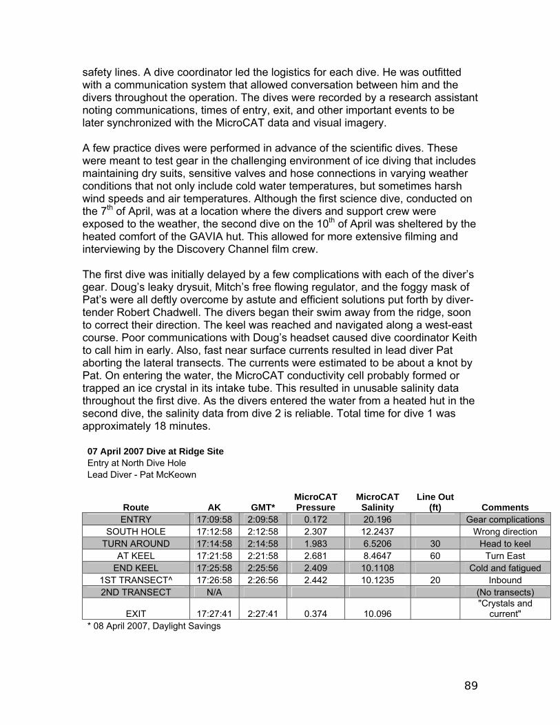
89

safety lines. A dive coordinator led the logistics for each dive. He was outfitted with a communication system that allowed conversation between him and the divers throughout the operation. The dives were recorded by a research assistant noting communications, times of entry, exit, and other important events to be later synchronized with the MicroCAT data and visual imagery. A few practice dives were performed in advance of the scientific dives. These were meant to test gear in the challenging environment of ice diving that includes maintaining dry suits, sensitive valves and hose connections in varying weather conditions that not only include cold water temperatures, but sometimes harsh wind speeds and air temperatures. Although the first science dive, conducted on the 7th of April, was at a location where the divers and support crew were exposed to the weather, the second dive on the 10th of April was sheltered by the heated comfort of the GAVIA hut. This allowed for more extensive filming and interviewing by the Discovery Channel film crew. The first dive was initially delayed by a few complications with each of the diver’s gear. Doug’s leaky drysuit, Mitch’s free flowing regulator, and the foggy mask of Pat’s were all deftly overcome by astute and efficient solutions put forth by diver-tender Robert Chadwell. The divers began their swim away from the ridge, soon to correct their direction. The keel was reached and navigated along a west-east course. Poor communications with Doug’s headset caused dive coordinator Keith to call him in early. Also, fast near surface currents resulted in lead diver Pat aborting the lateral transects. The currents were estimated to be about a knot by Pat. On entering the water, the MicroCAT conductivity cell probably formed or trapped an ice crystal in its intake tube. This resulted in unusable salinity data throughout the first dive. As the divers entered the water from a heated hut in the second dive, the salinity data from dive 2 is reliable. Total time for dive 1 was approximately 18 minutes. 07 April 2007 Dive at Ridge Site Entry at North Dive Hole Lead Diver - Pat McKeown

Route AK GMT* MicroCAT Pressure

MicroCAT Salinity

Line Out (ft) Comments

ENTRY 17:09:58 2:09:58 0.172 20.196 Gear complications SOUTH HOLE 17:12:58 2:12:58 2.307 12.2437 Wrong direction

TURN AROUND 17:14:58 2:14:58 1.983 6.5206 30 Head to keel AT KEEL 17:21:58 2:21:58 2.681 8.4647 60 Turn East

END KEEL 17:25:58 2:25:56 2.409 10.1108 Cold and fatigued 1ST TRANSECT^ 17:26:58 2:26:56 2.442 10.1235 20 Inbound 2ND TRANSECT N/A (No transects)

EXIT 17:27:41 2:27:41 0.374 10.096 "Crystals and

current" * 08 April 2007, Daylight Savings

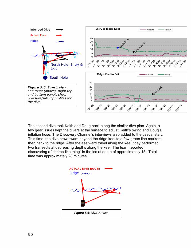
90

ACTUAL DIVE ROUTE

Ridge

The second dive took Keith and Doug back along the similar dive plan. Again, a few gear issues kept the divers at the surface to adjust Keith’s o-ring and Doug’s inflation hose. The Discovery Channel’s interviews also added to the casual start. This time, the dive crew swam beyond the ridge keel to a few green line markers, then back to the ridge. After the eastward travel along the keel, they performed two transects at decreasing depths along the keel. The team reported discovering a “shrimp-like thing” in the ice at depth of approximately 15’. Total time was approximately 28 minutes.

South Hole

North Hole, Entry & Exit

4

15

5

Intended Dive

Actual Dive

Ridge

Entry to Ridge Keel

Turn Arou

ndSou

th Hole

05

10152025

2:09:5

8

2:10:3

8

2:11:1

8

2:11:5

8

2:12:3

8

2:13:1

8

2:13:5

8

2:14:3

8

2:15:1

8

2:15:5

8

2:16:3

8

2:17:1

8

2:17:5

8

2:18:3

8

2:19:1

8

2:19:5

8

2:20:3

8

2:21:1

8

2:21:5

8

Pressure Salinity

Ridge Keel to Exit

End Kee

l

05

10152025

2:21:5

8

2:22:2

3

2:22:4

8

2:23:1

3

2:23:4

8

2:24:3

8

2:25:2

6

2:25:5

1

2:26:1

6

2:26:4

1

2:27:0

6

2:27:3

1

Pressure Salinity

Figure 5.5: Dive 1 plan, and route (above). Right top and bottom panels show pressure/salinity profiles for the dive.

Figure 5.6: Dive 2 route.

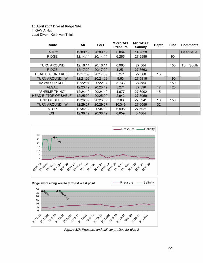
91

10 April 2007 Dive at Ridge Site In GAVIA Hut Lead Diver - Keith van Thiel

Route AK GMT MicroCAT Pressure

MicroCAT Salinity Depth Line Comments

ENTRY 12:09:19 20:09:19 0.064 14.7828 Gear issue RIDGE 12:14:14 20:14:14 6.265 27.5586 90

TURN AROUND 12:16:14 20:16:14 0.963 27.564 150 Turn South

RIDGE 12:17:29 20:17:29 4.251 27.5663 HEAD E ALONG KEEL 12:17:59 20:17:59 5.271 27.568 16

TURN AROUND - W 12:21:09 20:21:09 9.63 27.5816 190 1/2 WAY UP KEEL 12:22:04 20:22:04 5.733 27.584 150

ALGAE 12:23:49 20:23:49 5.271 27.596 17 120 "SHRIMP THING" 12:24:19 20:24:19 4.677 27.6002 15

HEAD E, "TOP OF SHELF" 12:25:09 20:25:09 2.942 27.5959 END OF SHELF 12:26:09 20:26:09 3.03 27.5941 10 150

TURN AROUND - W 12:29:27 20:29:27 10.349 27.6056 32 STOP 12:34:12 20:34:12 6.995 27.6021 EXIT 12:38:42 20:38:42 0.059 0.4064

Ridge

05

1015202530

20:09

:19

20:09

:44

20:10

:09

20:10

:34

20:10

:59

20:11

:24

20:11

:49

20:12

:14

20:12

:39

20:13

:04

20:13

:29

20:13

:54

20:14

:19

20:14

:44

20:15

:09

20:15

:34

20:15

:59

Pressure Salinity

RidgeSwim East

05

1015202530

20:17

:29

20:17

:44

20:17

:59

20:18

:14

20:18

:29

20:18

:44

20:18

:59

20:19

:14

20:19

:29

20:19

:44

20:19

:59

20:20

:14

20:20

:29

20:20

:44

20:20

:59

Pressure SalinityRidge swim along keel to farthest West point

Figure 5.7: Pressure and salinity profiles for dive 2

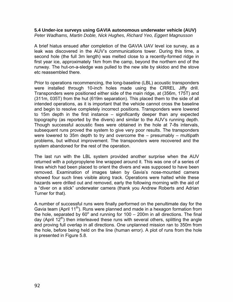
92

5.4 Under-ice surveys using GAVIA autonomous underwater vehicle (AUV) Peter Wadhams, Martin Doble, Nick Hughes, Richard Yeo, Eggert Magnusson A brief hiatus ensued after completion of the GAVIA UAV level ice survey, as a leak was discovered in the AUV’s communications tower. During this time, a second hole (the full 3m length) was melted close to a recently-formed ridge in first year ice, approximately 1km from the camp, beyond the northern end of the runway. The hut-on-a-sledge was pulled to the new site by skidoo and the stove etc reassembled there. Prior to operations recommencing, the long-baseline (LBL) acoustic transponders were installed through 10-inch holes made using the CRREL Jiffy drill. Transponders were positioned either side of the main ridge, at (356m, 175T) and (311m, 035T) from the hut (619m separation). This placed them to the side of all intended operations, as it is important that the vehicle cannot cross the baseline and begin to resolve completely incorrect positions. Transponders were lowered to 15m depth in the first instance – significantly deeper than any expected topography (as reported by the divers) and similar to the AUV’s running depth. Though successful acoustic fixes were obtained in the hole at 7-8s intervals, subsequent runs proved the system to give very poor results. The transponders were lowered to 35m depth to try and overcome the – presumably – multipath problems, but without improvement. The transponders were recovered and the system abandoned for the rest of the operation. The last run with the LBL system provided another surprise when the AUV returned with a polypropylene line wrapped around it. This was one of a series of lines which had been placed to orient the divers and was supposed to have been removed. Examination of images taken by Gavia’s nose-mounted camera showed four such lines visible along track. Operations were halted while these hazards were drilled out and removed, early the following morning with the aid of a “diver on a stick” underwater camera (thank you Andrew Roberts and Adrian Turner for that). A number of successful runs were finally performed on the penultimate day for the Gavia team (April 11th). Runs were planned and made in a hexagon formation from the hole, separated by 60o and running for 100 – 200m in all directions. The final day (April 12th) then interleaved these runs with several others, splitting the angle and proving full overlap in all directions. One unplanned mission ran to 350m from the hole, before being held on the line (human error). A plot of runs from the hole is presented in Figure 5.8.

93

An example of the resulting ice draft swath from one of these runs (22159, NE from the hole) is shown below in Figure 5.9.

Figure 5.9: An example swath of ice draft data, showing the main study ridge at the top of the picture and a thin, cracked, refrozen lead (draft =

0.6m) to the right.

Figure 5.8: Tracks of ice profiling runs done from the ridge site. The main study ridge lies approximately NW-

SE across the diagram

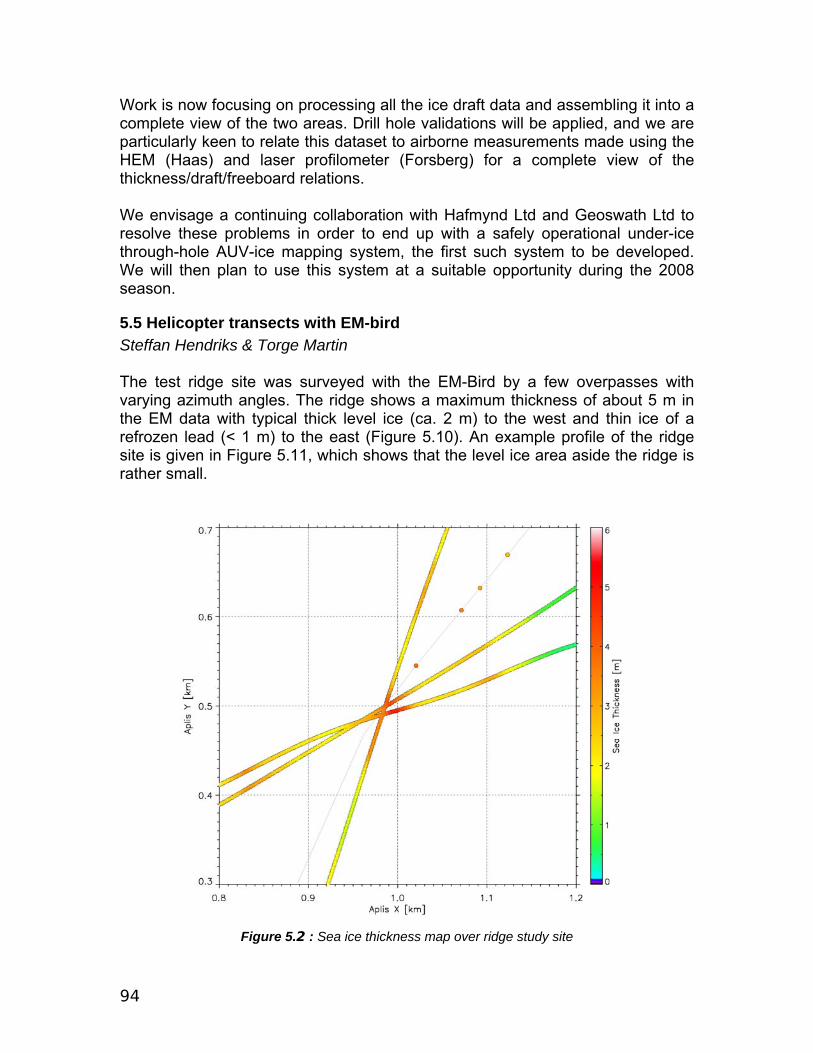
94

Work is now focusing on processing all the ice draft data and assembling it into a complete view of the two areas. Drill hole validations will be applied, and we are particularly keen to relate this dataset to airborne measurements made using the HEM (Haas) and laser profilometer (Forsberg) for a complete view of the thickness/draft/freeboard relations. We envisage a continuing collaboration with Hafmynd Ltd and Geoswath Ltd to resolve these problems in order to end up with a safely operational under-ice through-hole AUV-ice mapping system, the first such system to be developed. We will then plan to use this system at a suitable opportunity during the 2008 season.

5.5 Helicopter transects with EM-bird Steffan Hendriks & Torge Martin The test ridge site was surveyed with the EM-Bird by a few overpasses with varying azimuth angles. The ridge shows a maximum thickness of about 5 m in the EM data with typical thick level ice (ca. 2 m) to the west and thin ice of a refrozen lead (< 1 m) to the east (Figure 5.10). An example profile of the ridge site is given in Figure 5.11, which shows that the level ice area aside the ridge is rather small.

Figure 5.2 : Sea ice thickness map over ridge study site

95

Figure 5.3 : Example ridge profile with test ridge in the center of the figure

96

6. Perimeter Survey The ice camp was located on a multi-year ice floe, with a region of flat first year ice to the southwest where the runway was located. During the non-science camp large, kilometre wide leads opened to the North and South of the ice camp. These diverged and refroze. Later they became the sites of ridging and cracking, working throughout the science camp. A ridge formed, from the refrozen lead ice rafting onto thicker ice, to the north of camp on the evening of April 2nd. Part of this ridge became the ‘ridge study site’. Ridges formed to the east and west of the camp, just during the science camp. The ridge to the east of camp continuously worked, forming cracks on it’s east side. The other two ridges where less active. A lead (a.k.a. Pablo’s lead) close to the end of survey line 4, worked continuously throughout the science camp, closing, ridging and reopening several times. These four active features (cracks, leads and ridges) surrounded the camp, at times confined travel to within the area circumscribed by the leads and ridges. Hence they were defined as the perimeter of our in-situ study area. In the second week of camp, the first year ice the runway was situated on began to crack up, forming cracks and ridges between the APLIS camp and “Pablo’s lead” at the end of calibration transect line 3. There were numerous cracks in the first year ice between camp and Pablo’s lead that were not surveyed. In the short, 2 week, period of the ice camp it was not possible to do an in-depth survey of all the deformation features within snowmobile distance from camp. However, we were able to perform photographic surveys of all the active leads and ridges that surrounded the camp. These surveys will be used to estimate ridge volume and to pinpoint modes of dynamic activity we observe in satellite and buoy data. To expand results to the 10km scale, we may make the assumption that the ridges and leads at the “camp perimeter” were representative of similar features within the 10km buoy array. Satellite imagery will help us assess this assumption. 6.1 Photographic Survey of Dynamic ice Andrew Roberts & Jacqueline Richter-Menge A photographic survey of active sea ice features (leads, cracks & ridges) accessible from the ice camp (within a 2 mile radius), was performed. On April 6th, 20 survey sites were set up. Each site was chosen as it contained an interesting deformation feature that we expected would evolve dynamically. A whippy flag was place to mark the photographic subject, and a second whippy flag place 10 meters in front of the subject to mark the position of photographer. This ensured that repeat photographs of the same site where comparable. A 2m, 10cm marked post was held at the subject point in each photograph.

97

An example of a set of photographs for one site is shown in fig 6.1. Sites were visited every few days, if possible. Some site became inaccessible due to lead activity between the sites and camp. In particular some sites to the south of camp were only accessible once, as the first year ice in this vicinity started to break up in the first week of camp. Some other sites were put in later than April 6th, to compensate for the inaccessible sites. See appendix 6, table I for a list of available photographs for each site. These photographs may be viewed at http://research.iarc.uaf.edu/SEDNA/perimeter.php. Figure 6.2 shows the position of sites in appendix 6, table I, relative to command and control at the ice camp.

Figure 6.1: Example of Photographic survey for active site 2.0, which was located near the end of calibration transect line 2.

98

Figure 6.2: Photographic Sites for dynamic ice survey. Active sites are labled clockwise from

Ridge Site. The Active Site at the Ridge Site is labled 1.0, and sites between survey lines 1 and 2 are labled 1.1, 1.2, 1.3. Sites at the end of each Calibration Transect are labled x.0 where x is the calibration transect line number (1-6 clockwise from Ridge site), and a similar clockwise notation

is used for labelling active sites between calibration transects (x.1, x.2 etc.). These photographs will be analysed by an undergraduate summer student, to provide a detailed timeline of dynamic sea ice behaviour around the ice camp. The photographs are useful as anecdotal evidence for the nature and magnitude of specific deformation events we observed visually, in buoy track data and RADARSat image analysis. 6.2 Ridge Block Size Surveys Jennifer Hutchings & Alice Orlich Photographic surveys of the ridges to the north and east of camp were performed by Jennifer Hutchings, Pat McKeown, and Alice Orlich. We used a digital camera body (Olympus Evolt-500) with a 30mm Seiko lens and OM-10 to O/S lens adapter ring. In the centre of each photograph a 2m wooden post was placed close to the ridge. The post was painted with 10cm intervals. The intent of the photographs is to serve as a method of expediting block size data collection. Presumably, the photos will archive more block size dimensions than could be measured in-situ during a brief field campaign. The blocks can be measured later by viewing the image on a computer, using the painted 2m pole as a reference. Back at UAF, Alice Orlich analyzed the photographs, measuring the dimensions

99

of each visible block or portion thereof, in the image. The dimensions recorded were width(x), length(y), and depth(z) for each measurable block, as well as block volume, when (x), (y), and (z) for a block made it possible. Ridge height was also interpreted for the Ridge Site Calibration Survey. In relation to the ridge, (x) is the axis of the ridge, (y) is the axis crossing the ridge, and (z) accounts for the thickness of the block. 6.2.1 Ridge Site Calibration Survey Alice Orlich A series of photographs were taken on the 7th, 8th, and 10th of April at the first flag away from the ridge on each of site transects R1 through R6 (Figure 5.4.To estimate the accuracy of the photo-based data collection method, photographic measurements were compared to actual in-situ block size measurements at the Ridge Site (See 5.1 and Appendix 5, Table IV). As each photo was analyzed, comments were recorded as to the quality of the photo, perspective compared to others taken at same flag, and condition of ridge material, i.e rubble, blocks, snow cover, and dynamics. Block dimensions were taken only once for blocks appearing in multiple photographs so as not to include duplicate data points. Duplicate photos were only used for reference, but were counted into the Photo Efficiency Report (detailed below). The Ridge Site photo collection includes surveys for each day, facing both North (away from APLIS) and South (towards APLIS), so care was taken to not include the same blocks from different directions, but it was discovered that the photos sometimes revealed previously unseen blocks or provided better image quality due to varied sun position. Few blocks were immediate to the 2m measuring pole, so most of the measurements are estimated taking into account the distance from the pole. The photos were arranged by Ridge Site Line to compare with the in-situ measurements. It should be noted that the in-situ block measurements account for only the blocks that fell along where the transect line crossed, whereas the photos were taken at a distance away from the ridge, therefore including blocks between each line. For example, a photo of Ridge Site Line 2 would include blocks between Line 1 and Line 3. As noted earlier, duplicate blocks were attributed to only one Line data set. Due to the increase in blocks available in the photos, there was an average of 30% more data points found in the photos in comparison to the in-situ measurements. We found the mean dimensions of all blocks to vary between in-situ and photos by 42cm (x), 26cm (y), and 8cm (z). In addition, a Photo Efficiency Report was created to determine the effectiveness of the photo method to extract block size data. For evaluation purposes, a “data point” refers to any block dimension or ridge height measurable in a photo. The report concluded that of the 110 photos involved, 50.91% of them provided at least 1 data point, while 20.91% yielded multiple data points, implying that 49.09% were either duplicates or of poor quality. The complete block size comparison can be found at the following website: ??.

100

6.2.2 Perimeter Ridge Survey Alice Orlich This survey was conducted on two outlying ridges that appeared North (Jenny’s Ridge) and East (East Shear Ridge) of APLIS. Due to the distance involved in accessing the ridges, and the dynamic forces at work, the data collected was only photos, with no in-situ measurements accompanying them. The sites were visited on the 9th, 10th, 11th, 13th, and 14th of April. On any given day, one or both ridges were photographed at various locations . Photographs were taken at approximately 100m intervals along the ridges, the distance estimated by eye. The photographer took the image standing 10m in front of the 2m pole. The images were fewer in respect to distance covered when compared to the Ridge Site Calibration Survey. The photo collections for each ridge illustrated a great spectrum of features in both, considering that Jenny’s Ridge (JR) was a compression ridge, where large cube-shaped blocks would be expected, and the East Shear Ridge (ESR) was a shear ridge and therefore would be likely to produce more rubble and indiscernible block forms. In fact, when investigating the number of photos that included blocks, rubble, or snow cover or drifts, surprisingly both ridges had nearly equal amounts of blocks(JR=81%, ESR=88%) and rubble (JR= 36%, ESR=35%). Snow cover and drifts had a greater presence in the East Shear Ridge, with 58% of the photos hampered by it, where JR had only 12%. Very few blocks were immediate to the 2m measuring pole, so most of the measurements are estimated taking into account the distance from the pole. We found that the block size dimensions were not significantly different between the two ridges. The mean dimensions of all blocks vary between Jenny’s Ridge and the East Shear Ridge by 15cm (x), 16cm (y), and 6cm (z). A Photo Efficiency Report was also generated here, and it concluded that of the 50 photos involved, 32% of them provided at least 1 data point, while 20% yielded multiple data points, implying that 68% were either duplicates or of poor quality. The complete block size comparison can be found in Appendix 6, Table Ib. 6.2.3 Future Work After reviewing the data and statistics produced by the experiment, some new methods are proposed. Although the in-situ measurements provide a great sample for a ridge study, the method is time consuming and not entirely complete, as it was discovered that some blocks can not be measured on all axes due to overlap or submersion. It best serves as a quick, intense practice to gather a sample of a portion of a ridge. The photo survey proved to be helpful in yielding many additional data points, but which are subjective to the analyst’s perception. We suggest that the two methods continued to be administered in the field, but with a few modifications. When performing any ridge study, like was done on the Ridge Site portion of

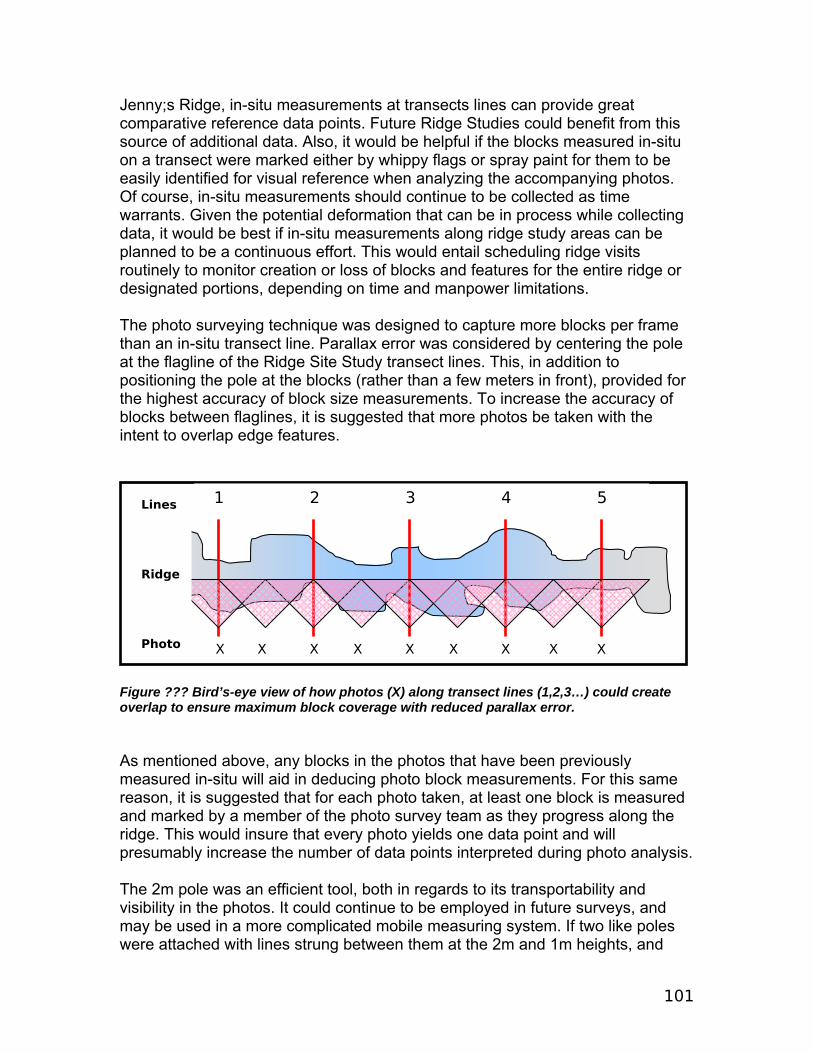
101

Jenny;s Ridge, in-situ measurements at transects lines can provide great comparative reference data points. Future Ridge Studies could benefit from this source of additional data. Also, it would be helpful if the blocks measured in-situ on a transect were marked either by whippy flags or spray paint for them to be easily identified for visual reference when analyzing the accompanying photos. Of course, in-situ measurements should continue to be collected as time warrants. Given the potential deformation that can be in process while collecting data, it would be best if in-situ measurements along ridge study areas can be planned to be a continuous effort. This would entail scheduling ridge visits routinely to monitor creation or loss of blocks and features for the entire ridge or designated portions, depending on time and manpower limitations. The photo surveying technique was designed to capture more blocks per frame than an in-situ transect line. Parallax error was considered by centering the pole at the flagline of the Ridge Site Study transect lines. This, in addition to positioning the pole at the blocks (rather than a few meters in front), provided for the highest accuracy of block size measurements. To increase the accuracy of blocks between flaglines, it is suggested that more photos be taken with the intent to overlap edge features.

Figure ??? Bird’s-eye view of how photos (X) along transect lines (1,2,3…) could create overlap to ensure maximum block coverage with reduced parallax error. As mentioned above, any blocks in the photos that have been previously measured in-situ will aid in deducing photo block measurements. For this same reason, it is suggested that for each photo taken, at least one block is measured and marked by a member of the photo survey team as they progress along the ridge. This would insure that every photo yields one data point and will presumably increase the number of data points interpreted during photo analysis. The 2m pole was an efficient tool, both in regards to its transportability and visibility in the photos. It could continue to be employed in future surveys, and may be used in a more complicated mobile measuring system. If two like poles were attached with lines strung between them at the 2m and 1m heights, and

1 2 3 4 5 Lines Ridge Photos

X X X X X X X X X

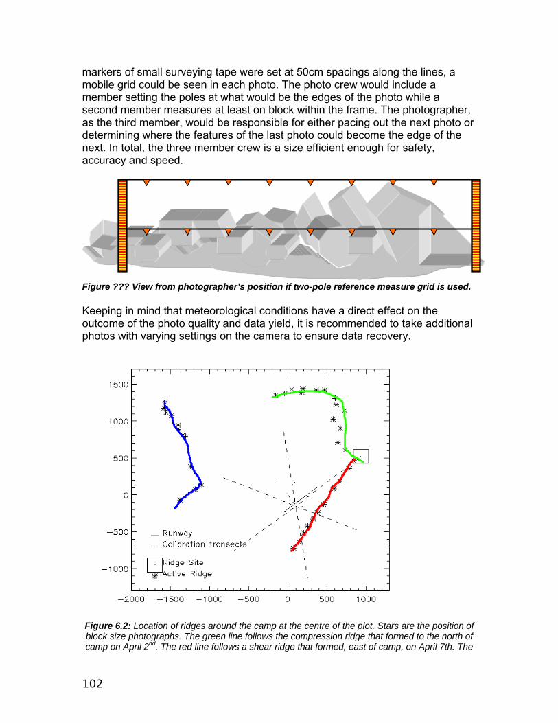
102

markers of small surveying tape were set at 50cm spacings along the lines, a mobile grid could be seen in each photo. The photo crew would include a member setting the poles at what would be the edges of the photo while a second member measures at least on block within the frame. The photographer, as the third member, would be responsible for either pacing out the next photo or determining where the features of the last photo could become the edge of the next. In total, the three member crew is a size efficient enough for safety, accuracy and speed.

Figure ??? View from photographer’s position if two-pole reference measure grid is used. Keeping in mind that meteorological conditions have a direct effect on the outcome of the photo quality and data yield, it is recommended to take additional photos with varying settings on the camera to ensure data recovery.

Figure 6.2: Location of ridges around the camp at the centre of the plot. Stars are the position of block size photographs. The green line follows the compression ridge that formed to the north of camp on April 2nd. The red line follows a shear ridge that formed, east of camp, on April 7th. The

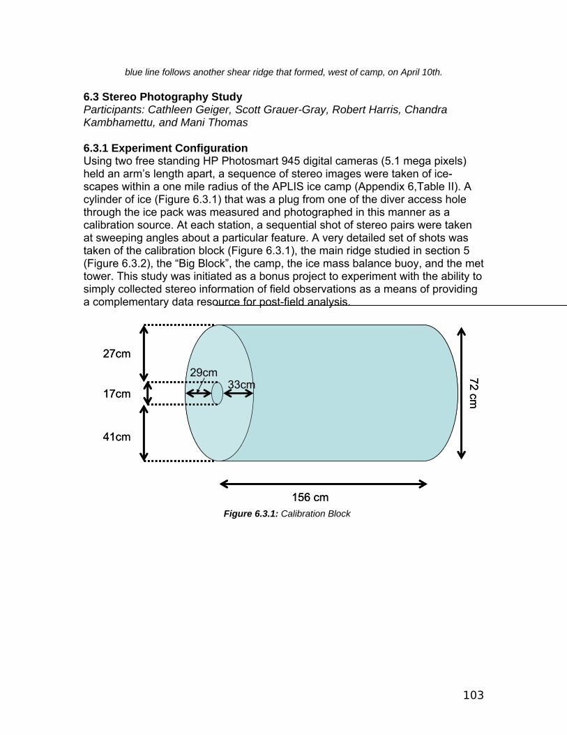
103

blue line follows another shear ridge that formed, west of camp, on April 10th. 6.3 Stereo Photography Study Participants: Cathleen Geiger, Scott Grauer-Gray, Robert Harris, Chandra Kambhamettu, and Mani Thomas 6.3.1 Experiment Configuration Using two free standing HP Photosmart 945 digital cameras (5.1 mega pixels) held an arm’s length apart, a sequence of stereo images were taken of ice-scapes within a one mile radius of the APLIS ice camp (Appendix 6,Table II). A cylinder of ice (Figure 6.3.1) that was a plug from one of the diver access hole through the ice pack was measured and photographed in this manner as a calibration source. At each station, a sequential shot of stereo pairs were taken at sweeping angles about a particular feature. A very detailed set of shots was taken of the calibration block (Figure 6.3.1), the main ridge studied in section 5 (Figure 6.3.2), the “Big Block”, the camp, the ice mass balance buoy, and the met tower. This study was initiated as a bonus project to experiment with the ability to simply collected stereo information of field observations as a means of providing a complementary data resource for post-field analysis.

156 cm

72 cm17cm

27cm

41cm

33cm29cm

156 cm

72 cm17cm

27cm

41cm

33cm29cm

Figure 6.3.1: Calibration Block

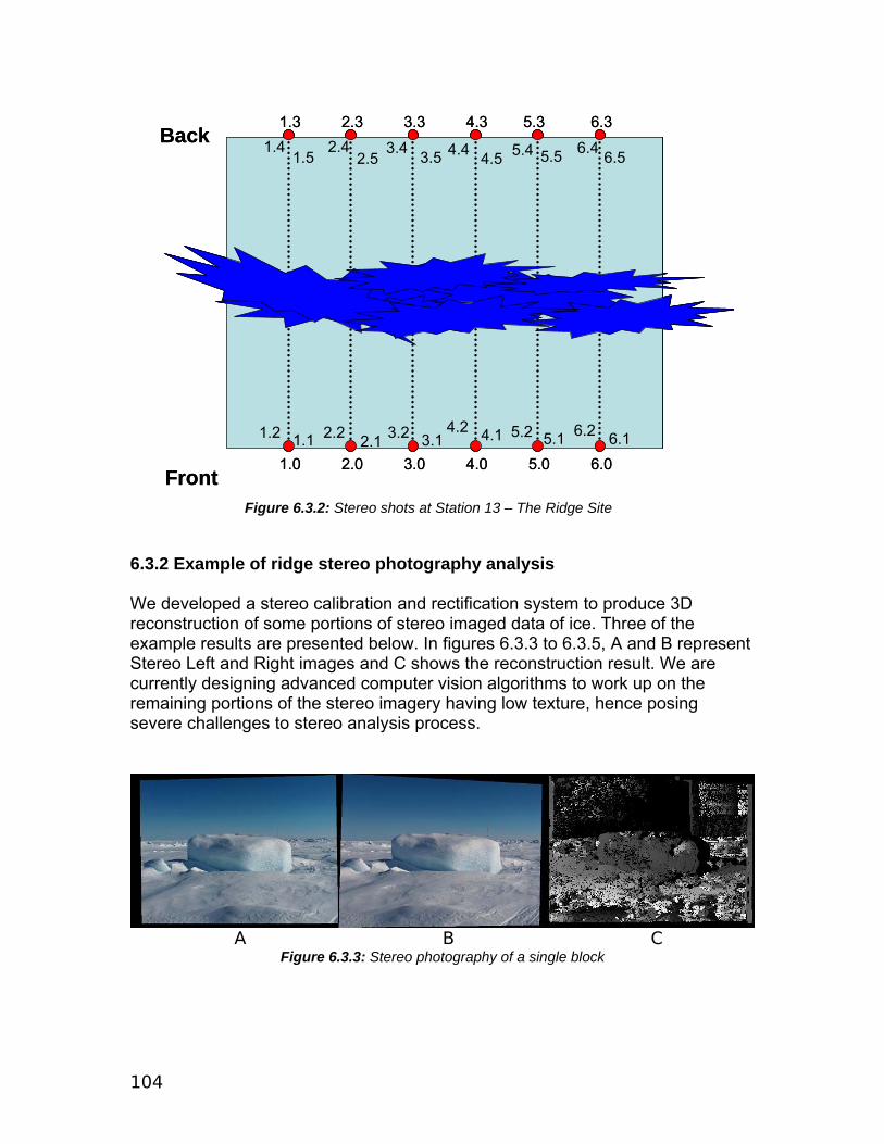
104

6.3.2 Example of ridge stereo photography analysis We developed a stereo calibration and rectification system to produce 3D reconstruction of some portions of stereo imaged data of ice. Three of the example results are presented below. In figures 6.3.3 to 6.3.5, A and B represent Stereo Left and Right images and C shows the reconstruction result. We are currently designing advanced computer vision algorithms to work up on the remaining portions of the stereo imagery having low texture, hence posing severe challenges to stereo analysis process.

A B C

Figure 6.3.3: Stereo photography of a single block

1.0

1.2 1.1 2.2 2.12.0 3.0 4.0 5.0 6.0

1.3 2.3 3.3 4.3 5.3 6.3

3.2 3.14.2 4.1 5.2 5.1 6.2 6.1

1.41.5

2.42.5

3.4 3.5 4.4 4.5 5.4 5.5 6.4 6.5

Front

Back

1.0

1.2 1.1 2.2 2.12.0 3.0 4.0 5.0 6.0

1.3 2.3 3.3 4.3 5.3 6.3

3.2 3.14.2 4.1 5.2 5.1 6.2 6.1

1.41.5

2.42.5

3.4 3.5 4.4 4.5 5.4 5.5 6.4 6.5

Front

Back

Figure 6.3.2: Stereo shots at Station 13 – The Ridge Site

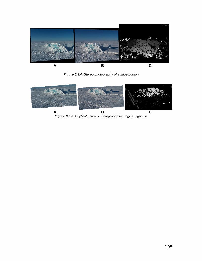
105

A B C

Figure 6.3.4: Stereo photography of a ridge portion

A B C

Figure 6.3.5: Duplicate stereo photographs for ridge in figure 4.

106

7. Meteorology

There were three separate groups of meteorological data collected during the SEDNA field campaign. Firstly, a weather station was erected at commencement of the SEDNA fieldwork and removed at the end of the campaign. This forms the most reliable and continuous set of atmospheric observations from the campaign. Secondly, observers recorded a rough set of cloud and precipitation observations to assist in the interpretation of satellite images and data from the SEDNA weather station. Finally, the Applied Physics Laboratory ice camp logged observations using an anemometer, wind vane, barometer and temperature sensors mounted approximately 6m above the command and control hut. Information on each of these data sources follows. 7.1 The SEDNA weather station Andrew Roberts

7.1.1 Introduction A SEDNA weather station was operated during the April 2007 field campaign to measure surface atmospheric variables necessary to estimate atmosphere-ice momentum fluxes. An annotated image of the station configuration appears in Figure 7.4. Wind speed and direction were measured with temperature and humidity 3.1 and 1.9 m above ground, in addition to barometric pressure and surface temperature. These were logged every ten minutes between April 2 2007, 05:50 and April 15 2007, 02:50 UTC. The weather station’s short 3m mast provided a robust instrument platform in strong winds, but the maximum measurement height of 3.1m precluded its use for estimating buoyant turbulent fluxes in the vicinity of leads, based on model results of Dare and Atkinson (1999) and Esau (2007). However the station was never within 400 meters of a lead and was of sufficient height to detect stably stratified surface conditions. Downward shortwave and longwave radiation fluxes were not measured because they are not of direct relevance to the sea ice momentum budget which was the focus of SEDNA campaign.

7.1.2 Weather Station Site The station was located on flat, multi-year sea ice more than 100m from recent ridge formations. No ridges formed within the vicinity during the field camp (Figure 7.4). Ice camp structures up to 4 meters high were more than 170 meters from the weather station, easily surpassing minimum WMO (2006) guidelines for structure and obstacle distances from a weather tower. The surface surrounding the weather station was covered with a mean snow depth of about 10cm during the recording period, varying spatially between bare ice and drifts approximately 30cm deep. Instrument heights quoted here were measured from the mean snow

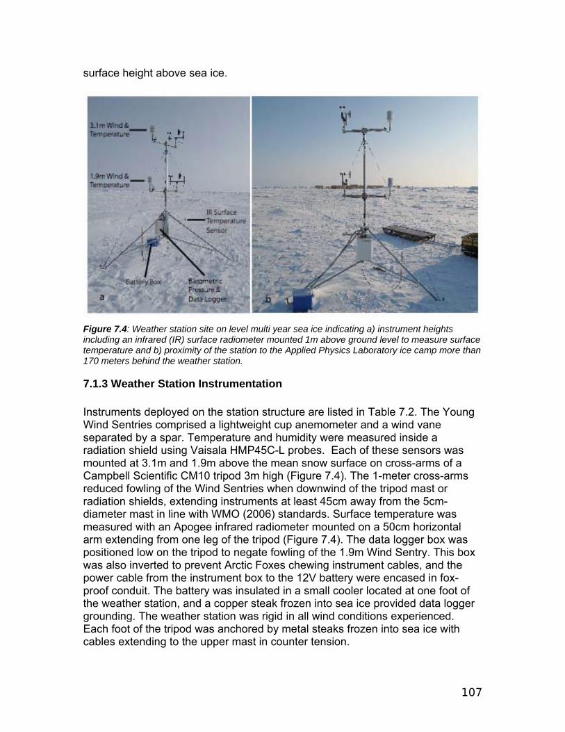
107

surface height above sea ice.

Figure 7.4: Weather station site on level multi year sea ice indicating a) instrument heights including an infrared (IR) surface radiometer mounted 1m above ground level to measure surface temperature and b) proximity of the station to the Applied Physics Laboratory ice camp more than 170 meters behind the weather station.

7.1.3 Weather Station Instrumentation Instruments deployed on the station structure are listed in Table 7.2. The Young Wind Sentries comprised a lightweight cup anemometer and a wind vane separated by a spar. Temperature and humidity were measured inside a radiation shield using Vaisala HMP45C-L probes. Each of these sensors was mounted at 3.1m and 1.9m above the mean snow surface on cross-arms of a Campbell Scientific CM10 tripod 3m high (Figure 7.4). The 1-meter cross-arms reduced fowling of the Wind Sentries when downwind of the tripod mast or radiation shields, extending instruments at least 45cm away from the 5cm-diameter mast in line with WMO (2006) standards. Surface temperature was measured with an Apogee infrared radiometer mounted on a 50cm horizontal arm extending from one leg of the tripod (Figure 7.4). The data logger box was positioned low on the tripod to negate fowling of the 1.9m Wind Sentry. This box was also inverted to prevent Arctic Foxes chewing instrument cables, and the power cable from the instrument box to the 12V battery were encased in fox-proof conduit. The battery was insulated in a small cooler located at one foot of the weather station, and a copper steak frozen into sea ice provided data logger grounding. The weather station was rigid in all wind conditions experienced. Each foot of the tripod was anchored by metal steaks frozen into sea ice with cables extending to the upper mast in counter tension.

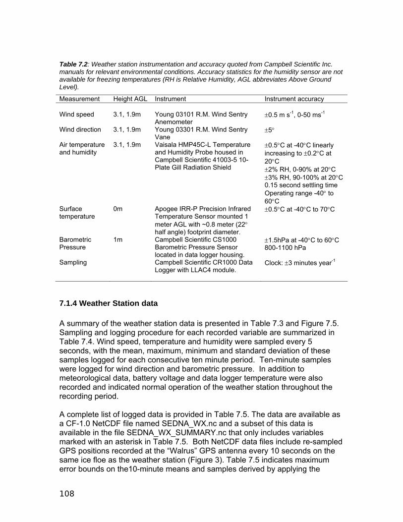
108

Table 7.2: Weather station instrumentation and accuracy quoted from Campbell Scientific Inc. manuals for relevant environmental conditions. Accuracy statistics for the humidity sensor are not available for freezing temperatures (RH is Relative Humidity, AGL abbreviates Above Ground Level).

Measurement Height AGL Instrument Instrument accuracy Wind speed 3.1, 1.9m Young 03101 R.M. Wind Sentry

Anemometer ±0.5 m s-1, 0-50 ms-1

Wind direction 3.1, 1.9m Young 03301 R.M. Wind Sentry Vane

±5°

Air temperature and humidity

3.1, 1.9m Vaisala HMP45C-L Temperature and Humidity Probe housed in Campbell Scientific 41003-5 10-Plate Gill Radiation Shield

±0.5°C at -40°C linearly increasing to ±0.2°C at 20°C ±2% RH, 0-90% at 20°C ±3% RH, 90-100% at 20°C 0.15 second settling time Operating range -40° to 60°C

Surface temperature

0m Apogee IRR-P Precision Infrared Temperature Sensor mounted 1 meter AGL with ~0.8 meter (22° half angle) footprint diameter.

±0.5°C at -40°C to 70°C

Barometric Pressure

1m Campbell Scientific CS1000 Barometric Pressure Sensor located in data logger housing.

±1.5hPa at -40°C to 60°C 800-1100 hPa

Sampling Campbell Scientific CR1000 Data Logger with LLAC4 module.

Clock: ±3 minutes year-1

7.1.4 Weather Station data A summary of the weather station data is presented in Table 7.3 and Figure 7.5. Sampling and logging procedure for each recorded variable are summarized in Table 7.4. Wind speed, temperature and humidity were sampled every 5 seconds, with the mean, maximum, minimum and standard deviation of these samples logged for each consecutive ten minute period. Ten-minute samples were logged for wind direction and barometric pressure. In addition to meteorological data, battery voltage and data logger temperature were also recorded and indicated normal operation of the weather station throughout the recording period. A complete list of logged data is provided in Table 7.5. The data are available as a CF-1.0 NetCDF file named SEDNA_WX.nc and a subset of this data is available in the file SEDNA_WX_SUMMARY.nc that only includes variables marked with an asterisk in Table 7.5. Both NetCDF data files include re-sampled GPS positions recorded at the “Walrus” GPS antenna every 10 seconds on the same ice floe as the weather station (Figure 3). Table 7.5 indicates maximum error bounds on the10-minute means and samples derived by applying the

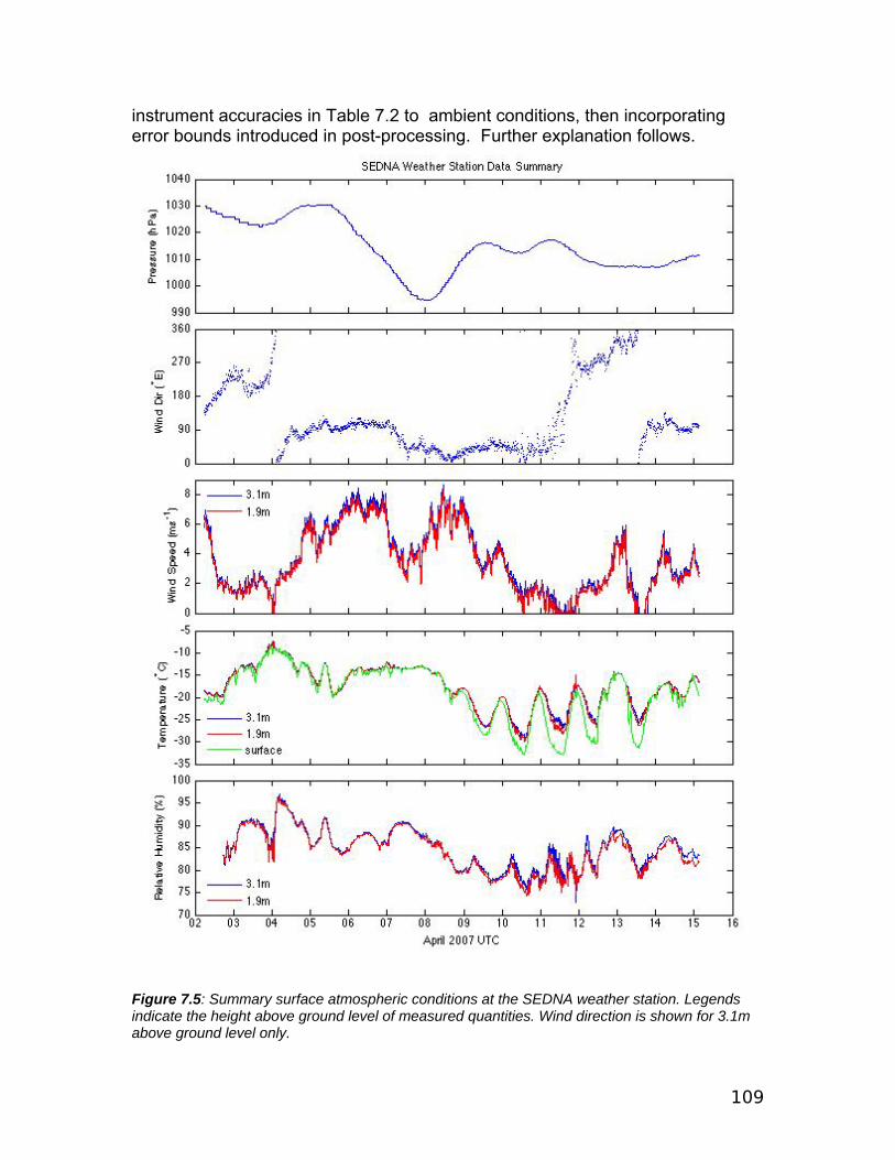
109

instrument accuracies in Table 7.2 to ambient conditions, then incorporating error bounds introduced in post-processing. Further explanation follows.

Figure 7.5: Summary surface atmospheric conditions at the SEDNA weather station. Legends indicate the height above ground level of measured quantities. Wind direction is shown for 3.1m above ground level only.

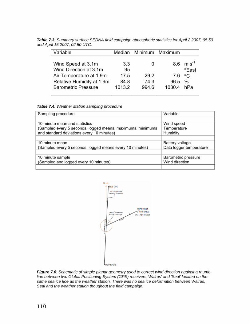
110

Table 7.3: Summary surface SEDNA field campaign atmospheric statistics for April 2 2007, 05:50 and April 15 2007, 02:50 UTC.

Variable Median Minimum Maximum Wind Speed at 3.1m 3.3 0 8.6 m s-1

Wind Direction at 3.1m 95 °East Air Temperature at 1.9m -17.5 -29.2 -7.6 °C Relative Humidity at 1.9m 84.8 74.3 96.5 % Barometric Pressure 1013.2 994.6 1030.4 hPa

Table 7.4: Weather station sampling procedure

Sampling procedure Variable 10 minute mean and statistics (Sampled every 5 seconds, logged means, maximums, minimums and standard deviations every 10 minutes)

Wind speed Temperature Humidity

10 minute mean (Sampled every 5 seconds, logged means every 10 minutes)

Battery voltage Data logger temperature

10 minute sample (Sampled and logged every 10 minutes)

Barometric pressure Wind direction

Figure 7.6: Schematic of simple planar geometry used to correct wind direction against a rhumb line between two Global Positioning System (GPS) receivers 'Walrus' and 'Seal' located on the same sea ice floe as the weather station. There was no sea ice deformation between Walrus, Seal and the weather station thoughout the field campaign.

111

The weather station was neither equipped with a Global Positioning System (GPS) receiver nor with a compass for determining absolute wind direction. Instead, the wind vane 0° reference direction was corrected against two fixed GPS receivers as illustrated in Figure 7.6. These two receivers, named ‘Walrus’ and ‘Seal’, sampled geographic position every 10 seconds throughout weather station operation. A 170m reference line was used to calculate a bearing of ~245°E for the 0° wind vane direction at 1900Z on April 3 2007. This was then used to correct the entire wind direction time series. There was a 4.6m error in handheld GPS position when establishing the 170m-reference line, resulting in directional error of ±3°. The positional error to the Walrus-Seal rhumb line introduces an additional error of ±2° (see introductory chapter of this report). The wind vane instrument error is ±5° (Table 7.2) giving a total wind direction error of ±10°. A more complicated wind direction correction is unlikely to yield significantly different results. Riming occurred on April 4 UTC and is evident in the sharp increase in relative humidity in Figure 7.5. Thin rime ice was deposited on all weather station instruments during this event. The affect of this was closely monitored by visual inspection, but did not appear to adversely affect any instrument’s operation. Both the wind vane and anemometer continued to rotate at the time of the riming event, even in light wind conditions (Figure 7.5). Rime ice gradually sublimed from instruments during the course of the day via solar heating. It is difficult to gauge the extent to which extra weight of rime affected recorded wind speed, but it is suggested instrument error bounds of ±0.5 m s-1 still apply for this segment of the data. Temperature retrievals from the Apogee radiometer could be adversely affected by blowing snow. However a brief analysis suggests there is no discernable correlation between 10-minute standard deviation of surface-temperature and 10-minute mean wind speed. Moreover, in windy conditions, surface temperature closely tracked air temperature (Figure 7.5), and blowing snow was infrequently observed more than 50cm above the surface. For this reason it is suggested the error bounds for surface temperature are within the instrument limits of ±0.5°C for the given environmental conditions. Due to a coding error, barometric pressure was logged to integer precision in hPa between 02-Apr-2007 05:50 and 03-Apr-2007 19:00 UTC, but was reset to log to three decimal places after this time. This affects the accuracy of relative humidity calculated from dew point; Relative humidity was not calculated and logged onboard until 02-Apr-2007 17:30, although dew point records extend throughout the time series. For this reason post-processed relative humidity values prior to 02-April 17:30 UTC have not been included in the station dataset to avoid publishing time series with variable quotable accuracy. Published relative humidity values have the same level of accuracy as quoted in Table 7.2.

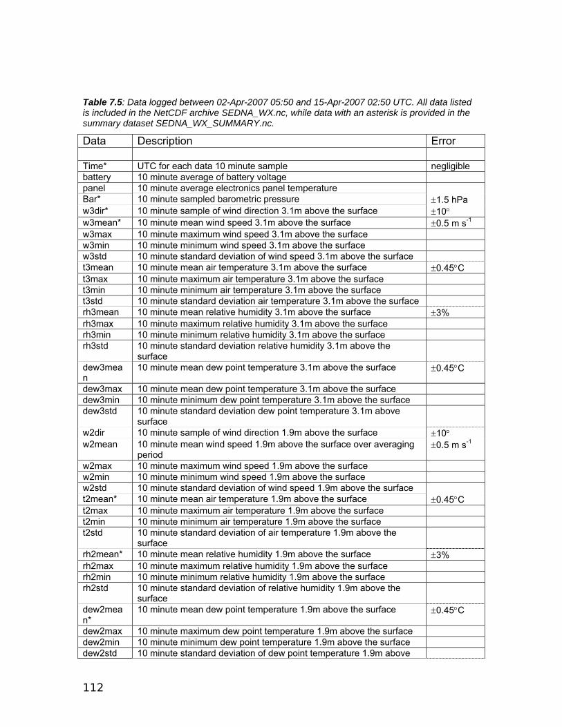
112

Table 7.5: Data logged between 02-Apr-2007 05:50 and 15-Apr-2007 02:50 UTC. All data listed is included in the NetCDF archive SEDNA_WX.nc, while data with an asterisk is provided in the summary dataset SEDNA_WX_SUMMARY.nc.

Data Description Error Time* UTC for each data 10 minute sample negligible battery 10 minute average of battery voltage panel 10 minute average electronics panel temperature Bar* 10 minute sampled barometric pressure ±1.5 hPa w3dir* 10 minute sample of wind direction 3.1m above the surface ±10° w3mean* 10 minute mean wind speed 3.1m above the surface ±0.5 m s-1

w3max 10 minute maximum wind speed 3.1m above the surface w3min 10 minute minimum wind speed 3.1m above the surface w3std 10 minute standard deviation of wind speed 3.1m above the surface t3mean 10 minute mean air temperature 3.1m above the surface ±0.45°C t3max 10 minute maximum air temperature 3.1m above the surface t3min 10 minute minimum air temperature 3.1m above the surface t3std 10 minute standard deviation air temperature 3.1m above the surface rh3mean 10 minute mean relative humidity 3.1m above the surface ±3% rh3max 10 minute maximum relative humidity 3.1m above the surface rh3min 10 minute minimum relative humidity 3.1m above the surface rh3std 10 minute standard deviation relative humidity 3.1m above the

surface

dew3mean

10 minute mean dew point temperature 3.1m above the surface ±0.45°C

dew3max 10 minute mean dew point temperature 3.1m above the surface dew3min 10 minute minimum dew point temperature 3.1m above the surface dew3std 10 minute standard deviation dew point temperature 3.1m above

surface

w2dir 10 minute sample of wind direction 1.9m above the surface ±10° w2mean 10 minute mean wind speed 1.9m above the surface over averaging

period ±0.5 m s-1

w2max 10 minute maximum wind speed 1.9m above the surface w2min 10 minute minimum wind speed 1.9m above the surface w2std 10 minute standard deviation of wind speed 1.9m above the surface t2mean* 10 minute mean air temperature 1.9m above the surface ±0.45°C t2max 10 minute maximum air temperature 1.9m above the surface t2min 10 minute minimum air temperature 1.9m above the surface t2std 10 minute standard deviation of air temperature 1.9m above the

surface

rh2mean* 10 minute mean relative humidity 1.9m above the surface ±3% rh2max 10 minute maximum relative humidity 1.9m above the surface rh2min 10 minute minimum relative humidity 1.9m above the surface rh2std 10 minute standard deviation of relative humidity 1.9m above the

surface

dew2mean*

10 minute mean dew point temperature 1.9m above the surface ±0.45°C

dew2max 10 minute maximum dew point temperature 1.9m above the surface dew2min 10 minute minimum dew point temperature 1.9m above the surface dew2std 10 minute standard deviation of dew point temperature 1.9m above

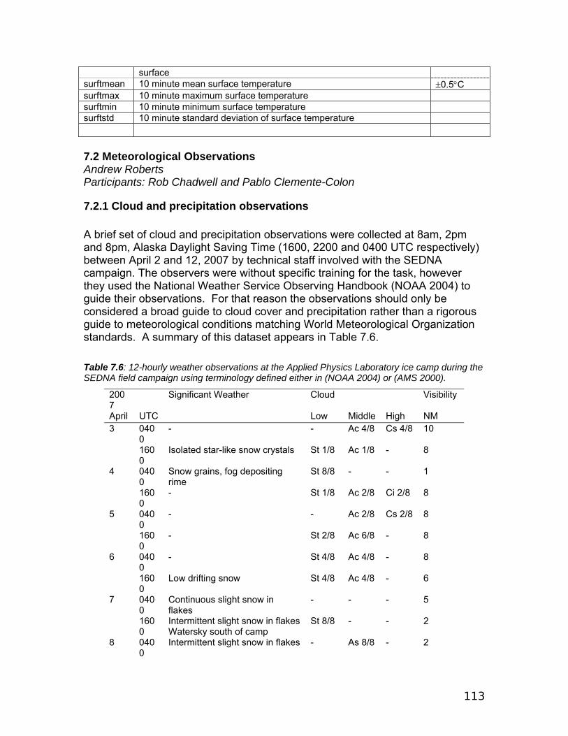
113

surface surftmean 10 minute mean surface temperature ±0.5°C surftmax 10 minute maximum surface temperature surftmin 10 minute minimum surface temperature surftstd 10 minute standard deviation of surface temperature 7.2 Meteorological Observations Andrew Roberts Participants: Rob Chadwell and Pablo Clemente-Colon

7.2.1 Cloud and precipitation observations A brief set of cloud and precipitation observations were collected at 8am, 2pm and 8pm, Alaska Daylight Saving Time (1600, 2200 and 0400 UTC respectively) between April 2 and 12, 2007 by technical staff involved with the SEDNA campaign. The observers were without specific training for the task, however they used the National Weather Service Observing Handbook (NOAA 2004) to guide their observations. For that reason the observations should only be considered a broad guide to cloud cover and precipitation rather than a rigorous guide to meteorological conditions matching World Meteorological Organization standards. A summary of this dataset appears in Table 7.6. Table 7.6: 12-hourly weather observations at the Applied Physics Laboratory ice camp during the SEDNA field campaign using terminology defined either in (NOAA 2004) or (AMS 2000).

2007

Significant Weather Cloud Visibility

April UTC Low Middle High NM 3 040

0 - - Ac 4/8 Cs 4/8 10

1600

Isolated star-like snow crystals St 1/8 Ac 1/8 - 8

4 0400

Snow grains, fog depositing rime

St 8/8 - - 1

1600

- St 1/8 Ac 2/8 Ci 2/8 8

5 0400

- - Ac 2/8 Cs 2/8 8

1600

- St 2/8 Ac 6/8 - 8

6 0400

- St 4/8 Ac 4/8 - 8

1600

Low drifting snow St 4/8 Ac 4/8 - 6

7 0400

Continuous slight snow in flakes

- - - 5

1600

Intermittent slight snow in flakes Watersky south of camp

St 8/8 - - 2

8 0400

Intermittent slight snow in flakes - As 8/8 - 2

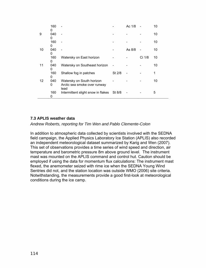
114

1600

- - Ac 1/8 - 10

9 0400

- - - - 10

1600

- - - - 10

10 0400

- - As 8/8 - 10

1600

Watersky on East horizon - - Ci 1/8 10

11 0400

Watersky on Southeast horizon - - - 10

1600

Shallow fog in patches St 2/8 - - 1

12 0400

Watersky on South horizon Arctic sea smoke over runway lead

- - - 10

1600

Intermittent slight snow in flakes St 8/8 - - 5

7.3 APLIS weather data Andrew Roberts, reporting for Tim Wen and Pablo Clemente-Colon In addition to atmospheric data collected by scientists involved with the SEDNA field campaign, the Applied Physics Laboratory Ice Station (APLIS) also recorded an independent meteorological dataset summarized by Karig and Wen (2007). This set of observations provides a time series of wind speed and direction, air temperature and barometric pressure 8m above ground level. The instrument mast was mounted on the APLIS command and control hut. Caution should be employed if using the data for momentum flux calculations: The instrument mast flexed, the anemometer seized with rime ice when the SEDNA Young Wind Sentries did not, and the station location was outside WMO (2006) site criteria. Notwithstanding, the measurements provide a good first-look at meteorological conditions during the ice camp.

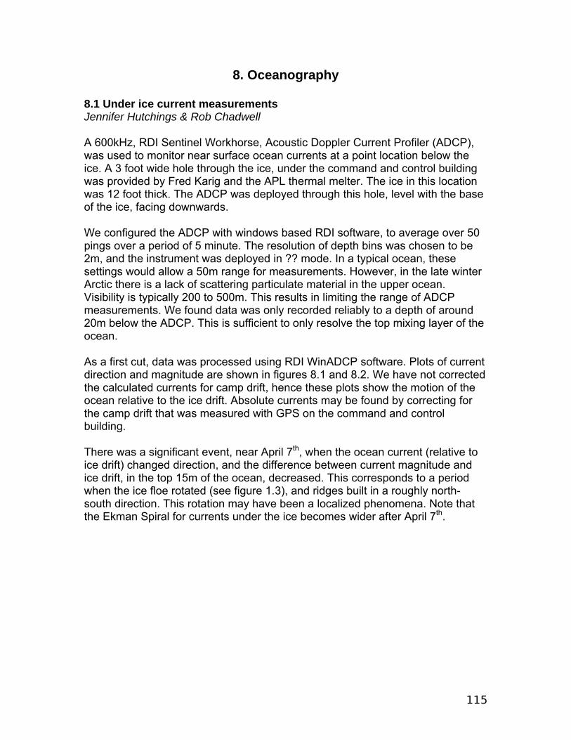
115

8. Oceanography

8.1 Under ice current measurements Jennifer Hutchings & Rob Chadwell A 600kHz, RDI Sentinel Workhorse, Acoustic Doppler Current Profiler (ADCP), was used to monitor near surface ocean currents at a point location below the ice. A 3 foot wide hole through the ice, under the command and control building was provided by Fred Karig and the APL thermal melter. The ice in this location was 12 foot thick. The ADCP was deployed through this hole, level with the base of the ice, facing downwards. We configured the ADCP with windows based RDI software, to average over 50 pings over a period of 5 minute. The resolution of depth bins was chosen to be 2m, and the instrument was deployed in ?? mode. In a typical ocean, these settings would allow a 50m range for measurements. However, in the late winter Arctic there is a lack of scattering particulate material in the upper ocean. Visibility is typically 200 to 500m. This results in limiting the range of ADCP measurements. We found data was only recorded reliably to a depth of around 20m below the ADCP. This is sufficient to only resolve the top mixing layer of the ocean. As a first cut, data was processed using RDI WinADCP software. Plots of current direction and magnitude are shown in figures 8.1 and 8.2. We have not corrected the calculated currents for camp drift, hence these plots show the motion of the ocean relative to the ice drift. Absolute currents may be found by correcting for the camp drift that was measured with GPS on the command and control building. There was a significant event, near April 7th, when the ocean current (relative to ice drift) changed direction, and the difference between current magnitude and ice drift, in the top 15m of the ocean, decreased. This corresponds to a period when the ice floe rotated (see figure 1.3), and ridges built in a roughly north-south direction. This rotation may have been a localized phenomena. Note that the Ekman Spiral for currents under the ice becomes wider after April 7th.

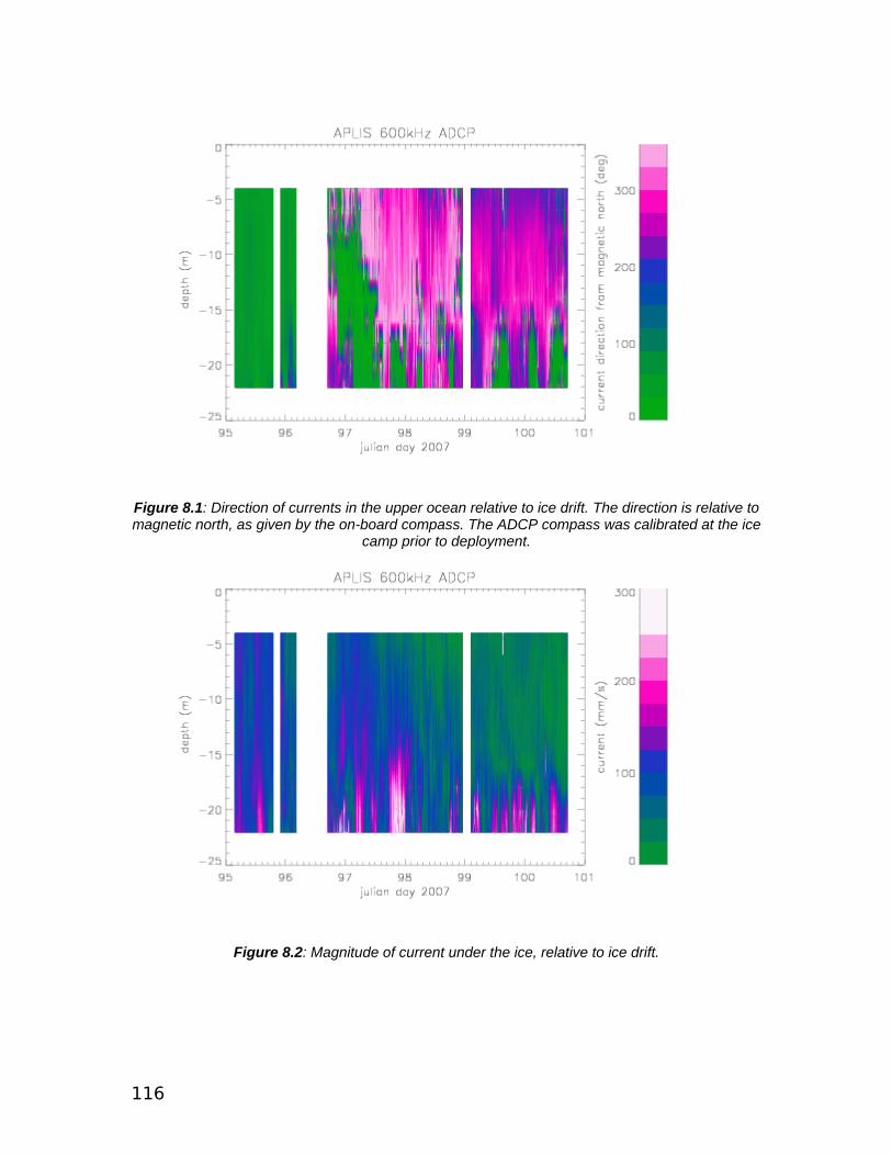
116

Figure 8.1: Direction of currents in the upper ocean relative to ice drift. The direction is relative to magnetic north, as given by the on-board compass. The ADCP compass was calibrated at the ice

camp prior to deployment.

Figure 8.2: Magnitude of current under the ice, relative to ice drift.

117

8.2 CTD casts Jeremy Wilkison

As mentioned previously, in the section entitled Tilt Meter Buoys, significant and accelerated change is occurring with respect to the sea ice in the Arctic Ocean. Coupled to these changes are modifications to the ocean structure. Therefore as part of the comprehensive data collection strategy at SEDNA/APLIS the structure of upper ocean of the Beaufort Sea was monitored. CTD casts were performed at approximately 6 hour intervals. The CTD used was the battery powered SEABIRD 19 which logs data to internal memory at 2Hz and carries its own internal clock. A pump-fed conductivity probe within the CTD carries out measurement of conductivity and temperature.

Once ‘on station’ the CTD was untied and readied for lowering through the

hydro-hole. Before entering the water the logging was initiated by positioning the switch to ‘on’ position. The lowering of the CTD into the water was generally a 2 person operation with one person operating the hand-winch, and the other ensuring the unit descended at a constant rate (< 1m/s). As it was not possible to ‘see’ the data in real time, all data was logged internally within the CTD, we performed two casts of the CTD at each station; just in case there was a malfunction in the unit during the first cast.

At the end of a station the CTD was lifted out of the water and stowed

away from the hydro-hole. The standard procedure for pumped SBE19 data processing, as recommended by SBE, was followed (cf. SBE SEASOFT manual). The table in appendix 7 lists the position, date, time and depth all CTD stations made during SEDNA.

An example of the data obtained can be seen in the figure below (up-and-down cast included).

Figure 8.3: Image of the hydro-hole used by the CTD to obtain the upper ocean structure

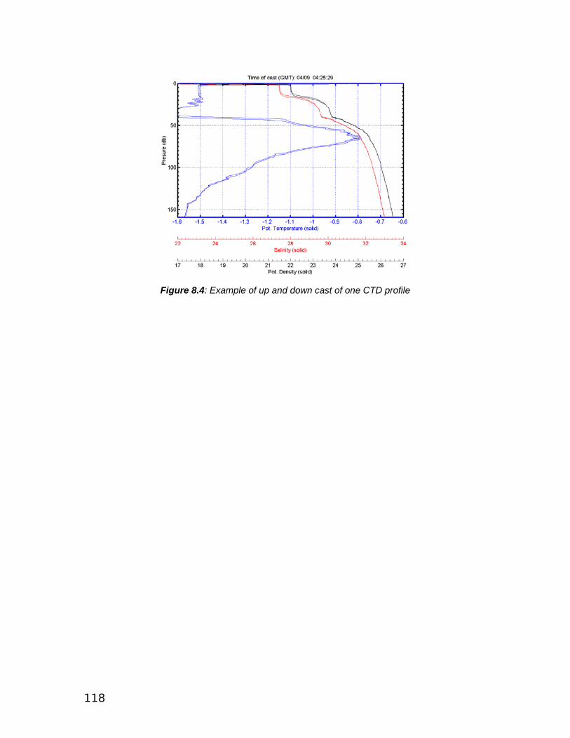
118

Figure 8.4: Example of up and down cast of one CTD profile

119

9. Outreach 9.1 PolarTrec Educational Outreach Robert Harris Part of the educational outreach program for the SEDNA Ice Camp consisted of embedding a high school science teacher, Robert Harris, from Hartford High School in White River Junction, Vermont into the camp. Mr. Harris participated as part of the PolarTREC program funded by the National Science Foundation. 9.1.1 Accomplishments: Prior to the ice camp. • Attended American Geophysical Union Annual meeting in San Francisco as a

guest of the SEDNA research team. • Mentioned in a newspaper article in the Connecticut Valley Spectator. • Contacted teachers in five Upper Connecticut Valley school districts

explaining the PolarTREC program and inviting their participation. • Presentations about the program and life in Alaska to Hartford School District.

Hour long presentations: 3/16 57 7th graders Hartford Middle School, 52 2nd graders Dothan Brook Elementary, 38 2nd graders Ottawaquechee Elementary, 3/19 65 1st & 2nd graders White River Elementary. 15 min long presentations: 3/19 17 High School Biology (Harris-Block 4 Grade 9), 3/20 18 (Archambault-Block 1 Grade 10),17 (Harris-Block 1 Grade 10), 18 (Harris-Block 2 Grade 10), 20 (Archambault-Block 3 Grade 10), 22 Physical Science (Archambault-Block 4 Grade 9).

• Travel to Alaska and attend the PolarTREC orientation and training (3/21-

25). • Bear Training and Firearms instruction (3/26). • Travel to Fort Yukon to do educational outreach (3/27-29). Met with Ms.

Jones, who invited us to Fort Yukon and visited her math classes. Met and talked with three of the village elders. Invited to attend the Spring Carnival, and crowning of the queen and court. Dr. Geiger and Mr. Harris both presented to 25 high school students and teachers.

• Worked at ARCUS, solving computer problems and up grading computer skills (3/30).

At the Ice Camp

• Arrived at the Ice camp (3/31) and actively participated to support the scientific mission as a member of the scientific party.

•

120

Wrote 14+ Journal entries and took a number of pictures about life at camp, which were down loaded via iridium satellite phone to be included in the PolarTREC website.

• Participated in a “Live event from IPY”, conference call from the ice. Which included Peggy Foletta, CA, Grade 10 Honors Biology, 25 students Bandon Gillette, KS, Grade 8 Earth Science, 25 students Jo Dodds, ID, Grade 9 Earth Science, 27 students Linda Cassassa, AK, Grade 7-12, 23 students Geoff Haines Stiles, NJ Hans Mueller, NH Lollie Garay, TX, Grade 5 science, 28 students Tania Giberyen, Luxembourg Lollie Garay, TX, Grade 5 science, 28 students Tania Giberyen, Luxembourg Kirk Beckendorf, TX, Grade and # students unknown

9.2 Sea Ice 101 9.2.1 Course Description: This is an upper level graduate and post doctoral level course (Mani and Scott being the only graduates and others being far more advanced), intended to give an idea of the various aspects of sea ice. In this course you will be given hands-on description of various kinds of ice and also have a chance to visit locations with different deformations. The lab section would be held in tandem with the lecture class. As part of the lab section, you would have a chance to play around on the ridges and drive the ski-doo. BE SURE TO DRESS WARM!!! Instructor: Jackie Richter-Menge Co-Instructor: Bruce Elder Class Hours: 8:30 am - 11:30 am, April 10th, 2007 Location: On the ice camp (within a 2 km radius) Office Hours: Maybe at CRREL, Hanover, but only by appointment... Textbook: Through word of mouth, so be sure to take notes since these things will not be repeated 9.2.2 Student’s Perspective by Mani Thomas Lecture 1:

The class covered the various formations that take place in the ice. The first thing that Jackie pointed out was the basic observational difference between first year and multi year ice. First year ice has a typical flat structure while multi year ice has significant undulations in them. Thus the air strip was built on first year ice while the camp in itself was located on multi year ice.

121

The first pit stop was at a lead that was due south west of the camp. A lead is an ice formation where a crack causes the ice to move apart. This lead was a significantly new one that had formed a couple of weeks ago. When observing leads, one thing that is typically observed is the presence of frost flowers. Frost flowers are structures that grow on frozen leads due to presence of superficial dents on the surface.

Lecture 2:

The next stop was at a multi year ice ridge. Ridges, unlike leads are formed due to ice hitting each other and creating a structure that is visible above the surface. Due to the properties of ice, the ratio of amount of ice that exists above the water to the ice that is below the water is about 1:4. This means that for every foot of ice that is visible above the surface, there is 4 feet of ice that is below the surface.

The crystals from multi year ice can be used for human consumption,

122

since the brine that is present in the water would have percolated into the water below, through the years of formation. When we observe the ice crystal, we can see a number of orifices within, where the brine percolated through.

When we look at the ridges present in multi year ice, they are found to

occur in two forms. The first is the compression ridge, which is created ice floes collides in a head-on fashion. Compression ridges typically have no shape and exist in a “cauliflower” kind of structure. The second type of ridge is the shearing ridge, which is created when floes move in opposite directions, rubbing against each other. Due to the rubbing motion, shearing ridges typically have a lot of polygonal structure associated with them.

The multi year ice contains many interspersed leads and ridges. In many

cases, leads drive right into a ridge dissipating their energy. This termination of a lead might create a brand new lead moving away from the ridge in a totally different direction. Also observable in close proximity to a ridge is the presence of basin-like structures on the ice. The creation of a ridge typically causes ice to start piling on top of one another and this causes a cantilever kind of conditions pushing one of the sides of the ridge down creating the basins.

123

A very interesting phenomenon that can be observed in the structures

present in the ice is the presence of brine stalactites (structures found hanging from the surface). These stalactites are created when the salt water trickles through the ice and freeze up when in contact with the -40F air.

Lecture 3:

From the location of the ridge, we proceeded to the region that was identified as the active zone for measurement purposes. This was the location where a significant amount of instrumentation was installed to obtain ground truth data regarding the ridge such as ridge height, water temperature and ridge keel shape.

Most of the measurements were collected by a combination of human divers and an Autonomous Underwater Vehicle (AUV). Prior to undertaking a dive, the human divers need to take a lot of precautionary steps. Typically, the

124

water under the ice is at -2F while the air is at -20F, so any water freezes up when it comes in contact with the air. To handle all these, the divers actually wear a suit (the red suit in the picture) that has an air insulation layer over and above the regular deep sea diving attire. This combination suit protects the divers from the severe cold temperature. I am not exactly sure how the buoyancy factor is tackled by the divers once they are inflated.

To handle the freezing up of water when in contact with the cold air, there is a "prep-hut" (the wooden box to the right) where the divers prepare themselves for the dive and thaw down after the dive.

The autonomous underwater vehicle is a robotic submarine manufactured

by Gavia in Ireland. The device is composed of multiple segments with a processor in each segment. Each segment performs the tack of capturing specific data such as side SAR, visible imagery, GPS information. The vehicle is released into the water through the hole (shown in the figure below) and specific way points are provided. The device autonomously visits the various waypoints, collecting data and once everything is accomplished would return to the “homing” location.

The first release for data collection went well but on its return journey it got stuck in a keel. To finally get it free, they had to release weights along the rope to which the AUV was tethered and pull it down from the keel. During this extraction, the GPS sensor and the central control were slightly damaged. In some cases, the AUV could get stuck pretty tightly and that would require divers to get in to the water so as to shake it loose.

125

9.3 Participating in Field Work – A remote sensors view point Katharine Giles The invitation to participate in the SEDNA project provided me with my first experience of seeing sea ice up close. As a remote sensor this was a truly invaluable experience. My work as a Post Doctoral Research Fellow, at University College London, involves studying Arctic and Antarctic sea ice by analysing data from the European Space Agency (ESA) satellites, ENVISAT and ERS 1 and 2. Living and working on the sea ice allowed me to see the range of ice types, ice thickness’ and snow depths that are present in relatively small area and provided inspiration for ideas to increase understanding of how a representative a satellite measurement of sea ice is, of the ice within its footprint. In addition I have also been involved with the Calibration/Validation discussions for the ESA satellite CryoSat. Participating in field work allowed me to get a real feel for what is and is not achievable in the field and the logistics of field work in a hostile environment, which I feel will be a very useful with regards to planning future calibration activities. Over all I am extremely grateful for this unique opportunity I have been given to live in such an amazing environment for two weeks and I feel that I have truly enhanced my understanding of sea ice and snow thanks to the enthusiasm of the PI’s and other scientists involved with SEDNA.

126

Acknowledgements SEDNA is an international collaboration funded by the National Science Foundation (NSF ARC 0612527, 0612105, 0611991). Matt Pruis is funded through NSF ARC 0612402. Robert Harris was supported by the ARCUS Polar-TREC program, funded by NSF. The Arctic Submarine Laboratory provided access to the Applied Physics Laboratory Ice Station, reducing field costs considerably. We express extensive thanks to Fred Karig and the team from the Applied Physics Laboratory who built and maintained the APLIS ice camp. The Alaska Satellite Facility (ASF) and National Ice Center facilitated near real time transfer of RADARSAT-1 ScanSAR-B imagery, provided by the Canadian Space Agency. We especially thank Melanie Engram at ASF for her enormous support during the near-real time portion of data acquisition. We thank NASA and ASF for providing this data for a full year, with full coverage of the Beaufort Sea. Airborne Lidar measurements was sponsored by the EU Damocles project. The Dash-8 overflight was supported by the Canadian Ice Service. Pablo Clemente-Colon provided scientific support and helped transition between the Navy and NSF periods of the ice camp. The International Arctic Buoy Program provided 3 meteorological buoys to enhance coverage in the Beaufort Sea, and is the central archive for all SEDNA buoy data.

127

128

APPENDIX 1

MODIS Images Acquired

Date Julian Day

TimeUTC

Satellite

Comments

15 March 2007 074 21:40 Aqua 16 March 2007 075 23:40 Terra 17 March 2007 076 22:45 Terra 18 March 2007 077 23:30 Terra 19 March 2007 078 22:35 Terra 20 March 2007 079 23:15 Terra 21 March 2007 080 22:20 Terra 22 March 2007 081 21:25 Terra 23 March 2007 082 20:50 Aqua Small leads, fairly random orientation. 24 March 2007 083 19:55 Aqua 25 March 2007 084 22:15 Aqua Initial development of shore lead along

Alaskan coast. Thin cloud. 26 March 2007 085 21:20 Aqua Major lead system running NW-SE parallel to

coast. 27 March 2007 086 22:35 Aqua 28 March 2007 087 20:50 Terra Shore lead at maximum state of development. 29 March 2007 088 21:50 Aqua NW-SE lead system closed. Curved lead

system in NW. 30 March 2007 089 22:35 Aqua Further curved lead systems running outward

from origin N of image. 31 March 2007 090 21:20 Terra Leads closing. 1 April 2007 091 22:00 Terra 2 April 2007 092 21:05 Terra 3 April 2007 093 21:50 Terra NW-SE lead reactivated. 4 April 2007 094 20:55 Terra Cloud 5 April 2007 095 23:15 Terra Cloud 6 April 2007 096 22:20 Terra More leads running NW-SE. 7 April 2007 097 21:25 Terra Cloud 8 April 2007 098 22:10 Terra Ice cover much more broken. Curved lead

systems. 9 April 2007 099 22:50 Terra Further ice break-up 10 April 2007 100 23:35 Terra Lattice pattern created by two sets of lead

orientations. 11 April 2007 101 22:40 Terra 12 April 2007 102 21:45 Terra Further break-up. Curved leads from open

water near Point Barrow. 13 April 2007 103 21:10 Aqua Cloud 14 April 2007 104 23:10 Terra Cloud cover over shore lead. Ice offshore very

broken. 15 April 2007 105 22:15 Terra Cloud cover over shore lead. Ice offshore very

broken.

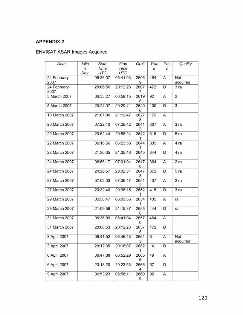
129

APPENDIX 2

ENVISAT ASAR Images Acquired

Date Julian

Day

Start Time UTC

Stop Time UTC

Orbit Track

Pass

Quality

24 February 2007

06:36:07 06:41:03 26069

464 A Not acquired

24 February 2007

20:06:56 20:12:26 26077

472 D 3 ra

5 March 2007 06:53:27 06:58:15 26198

92 A 2

5 March 2007 20:24:07 20:29:41 26206

100 D 3

10 March 2007 21:07:06 21:12:47 26278

172 A

20 March 2007 07:22:10 07:26:42 26413

307 A 3 ra

20 March 2007 20:52:44 20:58:24 26421

315 D 5 ra

22 March 2007 06:18:56 06:23:58 26441

335 A 4 ra

22 March 2007 21:30:05 21:35:46 26450

344 D 4 ra

24 March 2007 06:56:17 07:01:04 26470

364 A 2 ra

24 March 2007 20:26:57 20:32:31 26478

372 D 5 ra

27 March 2007 07:02:03 07:06:47 26513

407 A 2 ra

27 March 2007 20:32:40 20:38:15 26521

415 D 3 ra

29 March 2007 05:58:47 06:03:56 26541

435 A ra

29 March 2007 21:09:56 21:15:37 26550

444 D ra

31 March 2007 06:36:09 06:41:04 26570

464 A

31 March 2007 20:06:53 20:12:23 26578

472 D

3 April 2007 06:41:52 06:46:45 26613

6 A Not acquired

3 April 2007 20:12:35 20:18:07 26621

14 D

6 April 2007 06:47:38 06:52:29 26656

49 A

6 April 2007 20:18:20 20:23:53 26664

57 D

9 April 2007 06:53:23 06:58:11 26699

92 A

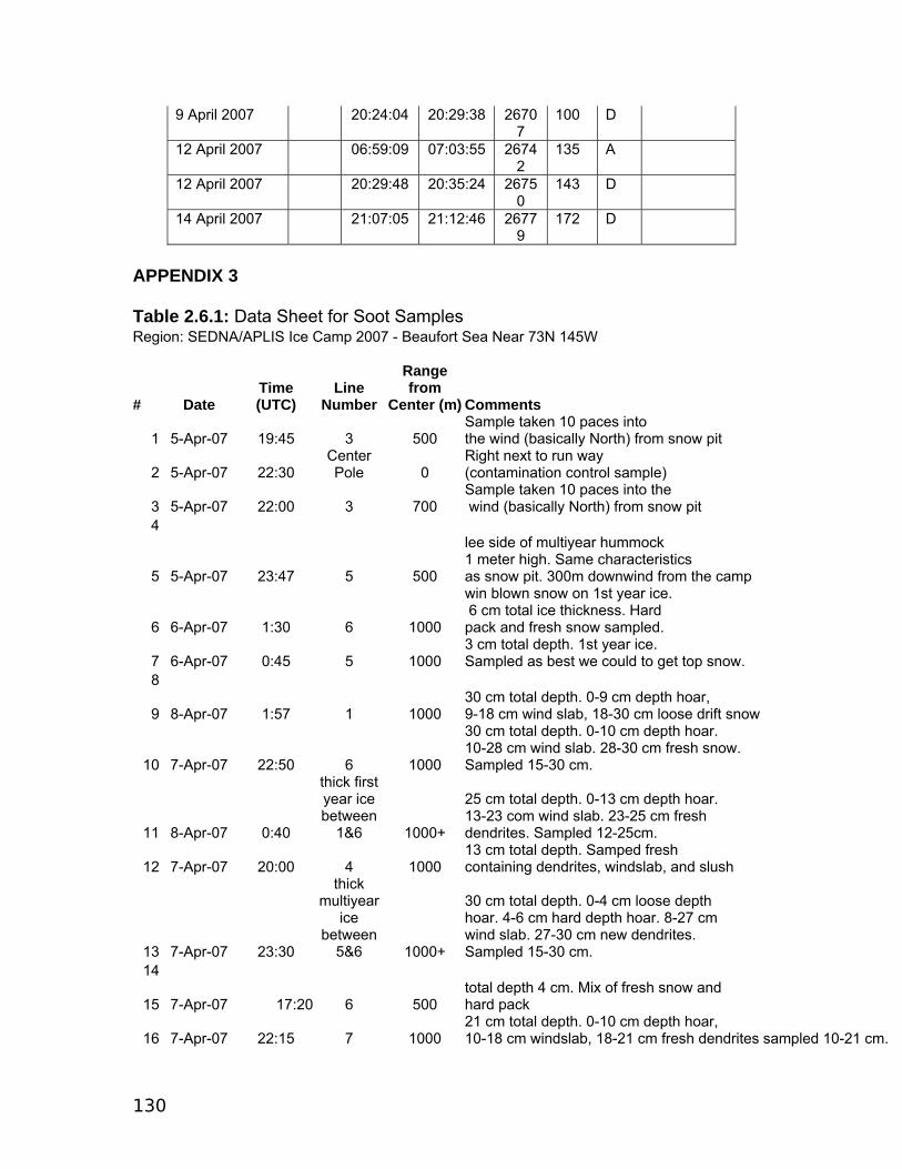
130

9 April 2007 20:24:04 20:29:38 26707

100 D

12 April 2007 06:59:09 07:03:55 26742

135 A

12 April 2007 20:29:48 20:35:24 26750

143 D

14 April 2007 21:07:05 21:12:46 26779

172 D

APPENDIX 3 Table 2.6.1: Data Sheet for Soot Samples Region: SEDNA/APLIS Ice Camp 2007 - Beaufort Sea Near 73N 145W

# Date Time (UTC)

Line Number

Range from

Center (m) Comments

1 5-Apr-07 19:45 3 500 Sample taken 10 paces into the wind (basically North) from snow pit

2 5-Apr-07 22:30 Center Pole 0

Right next to run way (contamination control sample)

3 5-Apr-07 22:00 3 700 Sample taken 10 paces into the wind (basically North) from snow pit

4

5 5-Apr-07 23:47 5 500

lee side of multiyear hummock 1 meter high. Same characteristics as snow pit. 300m downwind from the camp

6 6-Apr-07 1:30 6 1000

win blown snow on 1st year ice. 6 cm total ice thickness. Hard pack and fresh snow sampled.

7 6-Apr-07 0:45 5 1000 3 cm total depth. 1st year ice. Sampled as best we could to get top snow.

8

9 8-Apr-07 1:57 1 1000 30 cm total depth. 0-9 cm depth hoar, 9-18 cm wind slab, 18-30 cm loose drift snow

10 7-Apr-07 22:50 6 1000

30 cm total depth. 0-10 cm depth hoar. 10-28 cm wind slab. 28-30 cm fresh snow. Sampled 15-30 cm.

11 8-Apr-07 0:40

thick first year ice between

1&6 1000+

25 cm total depth. 0-13 cm depth hoar. 13-23 com wind slab. 23-25 cm fresh dendrites. Sampled 12-25cm.

12 7-Apr-07 20:00 4 1000 13 cm total depth. Samped fresh containing dendrites, windslab, and slush

13 7-Apr-07 23:30

thick multiyear

ice between

5&6 1000+

30 cm total depth. 0-4 cm loose depth hoar. 4-6 cm hard depth hoar. 8-27 cm wind slab. 27-30 cm new dendrites. Sampled 15-30 cm.

14

15 7-Apr-07 17:20 6 500 total depth 4 cm. Mix of fresh snow and hard pack

16 7-Apr-07 22:15 7 1000 21 cm total depth. 0-10 cm depth hoar, 10-18 cm windslab, 18-21 cm fresh dendrites sampled 10-21 cm.

131

17 8-Apr-07 19:00 2 500 3-4 cm total depth. 1 cm new snow, 2 cm hard pack. Sampling to 2 cm depth

18 7-Apr-07 22:00 7 500

Snow is a drift behind a hummock ~ 30cm total depth sampled top 15 cm. Top 3-4 cm is current snow. 15 cm thick windslab. 12 cm depth hoar. Sampled fresh snow and wind slab.

19 8-Apr-07 18:30 1 500

total depth > 20cm. Taking upper 10 cm upwind 60 paces from stake to avoid snow machine contamination. Sampled from 3 cm new snow and 7 cm hard pack.

20 8-Apr-07 19:20 2 1000 snow depth 20cm. 2-3 cm new snow, hard pack below. Sampling the upper 7cm.

APPENDIX 4: Wadhams et~al. thickness calibration data TABLE 1 Holes drilled along line of submarine submergence. For locations see fig. 3. Hole ice thickness Snow thicknesses Freeboard Distance

m nearby cm cm along line 1 1.63 6 5 4 24 0 2 1.94 28 18 27 7 50 3 6.81 9 8 13 38 125 4 3.73 4 3 4 50 150 5 1.83 7 10 1 14 200 6 1.79 2 3 2 18 250 7 4.48 28 26 44 26 300 8 2.29 70 -4 350 9 1.86 40 -2 400 10 2.85 21 19 18 30 450 11 1.85 25 8 500 12 3.92 11 10 8 38 550 13 2.00 34 33 30 1 625 14 2.60 52 50 0 650 15 1.70 40 9 700 16 0.79 28 27 30 10 800 17 2.67 38 21 850 18 1.31 13 11 12 11 At barrel 19 1.40 12 12 10 13 At barrel 20 1.35 10 8 10 10 At barrel 21 1.39 8 7 13 11 At barrel Notes: 1. Hole numbers begin with hole 1 which is estimated to be 23 m down-track

132

from surfacing location of submarine’s bow. 2. Holes 18 – 21 were a quadrilateral (3-4 m side) drilled neat the marker barrel to give ice thickness on what was the south side of the lead at the time of surfacing. 3. Where distances between holes are irregular it is because a ridge or rubble field intervened – see map. 4. Negative freeboard indicates flooded ice. TABLE II Grid of holes drilled around Gavia hut at first position. Holes are numbered by row and column in same orientation as the map in fig. 5, and are 10 m apart. Three snow depths were sampled at each hole position. ICE THICKNESS (To Ice-Snow Interface) 1 2 3 4 5 6 7 8 9 10 11

1 156 160 150 139 150 146 149 140 114 170 138 2 142 152 158 163 144 156 163 154 160 147 166 3 142 152 149 161 149 160 172 145 128 136 168 4 159 146 146 164 148 164 157 131 181 139 154 5 133 155 175 163 151 172 164 143 157 144 137 6 148 162 162 154 161 167 164 140 166 221 132 7 138 158 151 152 122 152 167 132 167 131 132 8 137 116 146 139 145 163 170 140 128 145 137 9 136 145 147 168 196 153 169 148 163 141 136

10 119 143 158 170 162 154 177 147 147 137 150 11 129 113 174 163 161 150 167 160 151 148 129 12 149 129 183 183 154 135 172 143 147 129 13 139

FREEBOARD Top of Ice - Ice-Snow Interface 1 2 3 4 5 6 7 8 9 10 11

1 21 22 18 13 19 16 18 15 11 22 12 2 13 13 14 13 14 14 11 18 13 11 17 3 13 13 14 13 14 14 13 11 6 8 30 4 13 11 12 13 14 14 14 4 10 4 16 5 10 11 18 12 14 15 16 12 12 4 5 6 13 15 14 12 15 14 10 9 6 27 8 7 8 11 9 7 4 11 10 7 20 3 9 8 9 6 2 3 11 14 12 10 3 12 12 9 9 9 4 2 26 14 14 12 17 10 13

10 8 7 5 16 15 14 16 12 10 11 14 11 10 5 18 8 16 15 5 12 15 11 8

133

12 14 8 11 16 14 9 13 13 15 12 13 10

SNOW DEPTH 1 1 2 3 4 5 6 7 8 9 10 11

1 4.5 9 5 12 8 17 16 14 40 29 7 2 8 7 6 4 14 9 5 7 8 9 4 3 6 6 7 8 8 6 5 10 19 35 1 4 12 13 24 5 9 18 2 40 28 35 8 5 16 6 6 12 6 7 6 8 16 55 23 6 4 8 5 12 25 2 12 10 35 36 19 7 9 14 19 15 16 11 14 20 24 10 12 8 5 33 30 31 21 10 10 13 22 10 17 9 12 16 15 9 16 11 7 10 10 8 13

10 18 13 5 9 10 7 16 13 20 8 7 11 8 31 28 22 6 7 16 23 9 9 14 12 13 14 18 14 12 4 20 4 7 16 13 14

SNOW DEPTH 2 1 2 3 4 5 6 7 8 9 10 11

1 4.5 11 5 11 8 20 14 10 36 29 12 2 8 6 5 5 15 8 5 7 12 12 3 3 5 5 9 8 9 6 4 8 18 30 1 4 12 21 25 6 9 13 9 40 28 32 19 5 20 7 5 12 6 9 4 7 16 49 22 6 7 5 4 14 26 7 11 11 38 33 19 7 8 13 21 14 17 11 14 14 24 18 11 8 4 31 30 33 27 7 11 6 26 10 20 9 13 16 15 7 0 9 10 11 12 8 15

10 23 16 7 19 13 5 16 8 20 9 7 11 8 30 20 21 8 7 21 14 9 7 13 12 15 14 18 9 11 6 14 6 7 18 13 12

SNOW DEPTH 3 1 2 3 4 5 6 7 8 9 10 11

1 5 11 5 10 7 10 8 9 34 22 7

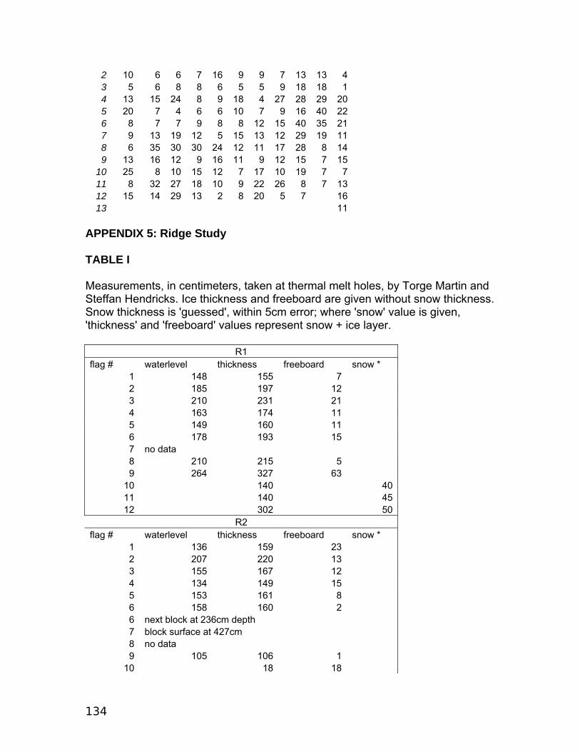
134

2 10 6 6 7 16 9 9 7 13 13 4 3 5 6 8 8 6 5 5 9 18 18 1 4 13 15 24 8 9 18 4 27 28 29 20 5 20 7 4 6 6 10 7 9 16 40 22 6 8 7 7 9 8 8 12 15 40 35 21 7 9 13 19 12 5 15 13 12 29 19 11 8 6 35 30 30 24 12 11 17 28 8 14 9 13 16 12 9 16 11 9 12 15 7 15

10 25 8 10 15 12 7 17 10 19 7 7 11 8 32 27 18 10 9 22 26 8 7 13 12 15 14 29 13 2 8 20 5 7 16 13 11

APPENDIX 5: Ridge Study TABLE I Measurements, in centimeters, taken at thermal melt holes, by Torge Martin and Steffan Hendricks. Ice thickness and freeboard are given without snow thickness. Snow thickness is 'guessed', within 5cm error; where 'snow' value is given, 'thickness' and 'freeboard' values represent snow + ice layer.

R1 flag # waterlevel thickness freeboard snow *

1 148 155 7 2 185 197 12 3 210 231 21 4 163 174 11 5 149 160 11 6 178 193 15 7 no data 8 210 215 5 9 264 327 63

10 140 4011 140 4512 302 50

R2 flag # waterlevel thickness freeboard snow *

1 136 159 23 2 207 220 13 3 155 167 12 4 134 149 15 5 153 161 8 6 158 160 2 6 next block at 236cm depth 7 block surface at 427cm 8 no data 9 105 106 1

10 18 18

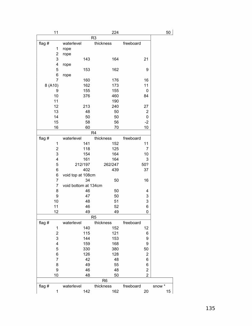
135

11 224 50R3

flag # waterlevel thickness freeboard 1 rope 2 rope 3 143 164 21 4 rope 5 153 162 9 6 rope 7 160 176 16

8 (A10) 162 173 11 9 155 155 0

10 376 460 84 11 190 12 213 240 27 13 48 50 2 14 50 50 0 15 58 56 -2 16 60 70 10

R4 flag # waterlevel thickness freeboard

1 141 152 11 2 118 125 7 3 154 164 10 4 161 164 3 5 212/197 262/247 50? 6 402 439 37 6 void top at 108cm 7 34 50 16 7 void bottom at 134cm 8 46 50 4 9 47 50 3

10 48 51 3 11 46 52 6 12 49 49 0

R5 flag # waterlevel thickness freeboard

1 140 152 12 2 115 121 6 3 144 153 9 4 159 168 9 5 330 380 50 6 126 128 2 7 42 48 6 8 49 55 6 9 46 48 2

10 48 50 2 R6

flag # waterlevel thickness freeboard snow * 1 142 162 20 15

136

2 130 169 39 253 194 219 25 204 231 239 8 205 22 30 8 5 126 125 -1 6 147 147 0 7 132 144 12 8 132 145 13 8 block of 10cm thickness rafted ontop

TABLE II Two inch auger holes were drill for three locations (a,b,c on figure ??) that extended calibration transect 1 to ridge transect R3. Peter Wadhams recorded thickness measurements at these points. Hole Snow freeboard thcknessa 24,17,19 12 2.51b 3,2,2 15 1.6c 5,5,4 13 1.63

TABLE III Two inch auger holes were drilled through ridge, to augment measurements made with the CRREL thermal melter. The holes were drilled along 4m lines perpendicular to thermal melt holes through the ridge along transects R1, R3 and R6. These measurements were performed by Katharine Giles, Alice Orlich, Adrian Turner, Jennifer Hutchings and Pablo Clemente-Colon. Voids hole number dist. To bottom of void dist. To top of void snow depth total depth comments

6.1 2.3 2.5 0.5 5.1 6.2 1.54 0.76 0.56 6.3 6.3 2.2 1.85 0.46 7.64 6.4 0.01 7.8 no voids 6.5 1.8 1.4 0.01

7.8 7.57 8.0 - 8.5

could not measure bottodepth estimated using drfilghts

3.1 0.51 0.5 0.01 2.54

3.2 2.7 1.8 3.0 - 3.50

could not measure bottodepth estimated using drfilghts

3.3 3 2.67 0.03 4.82 3.4 2.5 2.3 0.01 4.3 3.5 0.08 0.6 0.01 4.52 3.6 0.9 0.52 0.01 4.83 3.7 3.27 no voids 3.8 1.3 1.13 0.14 2.92

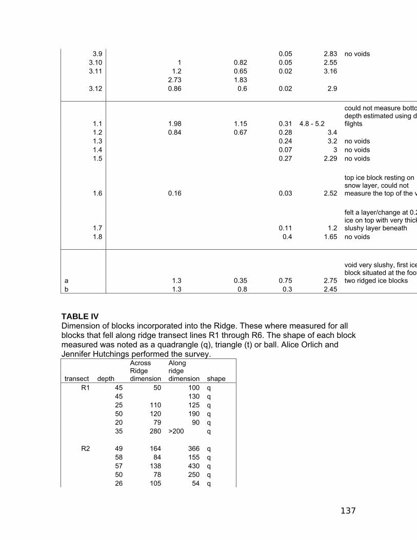
137

3.9 0.05 2.83 no voids 3.10 1 0.82 0.05 2.55 3.11 1.2 0.65 0.02 3.16

2.73 1.83 3.12 0.86 0.6 0.02 2.9

1.1 1.98 1.15 0.31 4.8 - 5.2

could not measure bottodepth estimated using drfilghts

1.2 0.84 0.67 0.28 3.4 1.3 0.24 3.2 no voids 1.4 0.07 3 no voids 1.5 0.27 2.29 no voids

1.6 0.16 0.03 2.52

top ice block resting on snow layer, could not measure the top of the v

1.7 0.11 1.2

felt a layer/change at 0.2ice on top with very thickslushy layer beneath

1.8 0.4 1.65 no voids

a 1.3 0.35 0.75 2.75

void very slushy, first iceblock situated at the foottwo ridged ice blocks

b 1.3 0.8 0.3 2.45

TABLE IV Dimension of blocks incorporated into the Ridge. These where measured for all blocks that fell along ridge transect lines R1 through R6. The shape of each block measured was noted as a quadrangle (q), triangle (t) or ball. Alice Orlich and Jennifer Hutchings performed the survey.

transect depth

Across Ridge dimension

Along ridge dimension shape

R1 45 50 100 q 45 130 q 25 110 125 q 50 120 190 q 20 79 90 q 35 280 >200 q

R2 49 164 366 q 58 84 155 q 57 138 430 q 50 78 250 q 26 105 54 q

138

R3 37 34 25 q

44 143 144 t 15 56 40 q 60 190 230 q 48 57 49 q 8 32 36 q 10 46 33 q 54 145 200 q 60 60 58 t 18 24 40 q 48 50 70 ball 55 128 154 q

R4 50 160 270 q 30 42 40 q 35 55 93 q 50 129 90 t

R5 10 60 160 q 40 61 q 48 220 235 q

R6 36 115 150 q 33 167 190 q

APPENDIX 6: Perimeter survey TABLE I All photographs available in active site survey around camp. Site Lable date

time (gmt)

lat (deg N)

lat (min N)

long (deg W)

long (deg W) photographer

1.0 4/6 19:04 73 20.422 145 57.751 JRM 1.0 4/14 0:00 73 11.631 146 35.399 AR 1.1 4/11 3:48 73 11.564 146 40.227 JH 1.1 4/6 19:40 73 20.274 145 58.475 JRM 1.1 4/14 0:02 73 11.469 146 35.62 AR 1.2 4/6 20:21 73 20.089 145 59.305 JRM 1.2 4/14 0:06 73 11.264 146 35.887 AR 1.3 4/6 20:57 73 19.985 145 59.094 JRM 2 4/12 0:58 73 11.11 146 39.993 JH 2.0 4/7 2:52 73 20.222 146 5.01 JRM 2.1 4/12 1:54 73 11.116 146 39.893 JH 2.1 4/7 2:43 73 20.222 146 5.005 JRM 2.2 4/12 2:05 73 11.304 146 39.08 JH 2.2 4/12 0:49 73 11.055 146 40.516 JH 2.2 4/7 2:26 73 20.154 146 5.338 JRM 2.2A 4/12 0:49 73 11.055 146 40.516 JH 3 4/12 0:42 73 11.034 146 40.998 JH 3.0 4/7 2:07 73 20.125 146 5.648 JRM

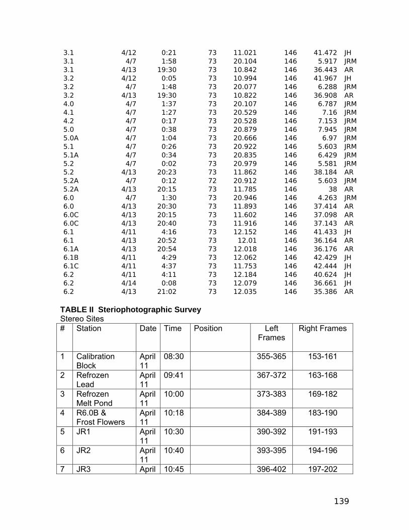
139

3.1 4/12 0:21 73 11.021 146 41.472 JH 3.1 4/7 1:58 73 20.104 146 5.917 JRM 3.1 4/13 19:30 73 10.842 146 36.443 AR 3.2 4/12 0:05 73 10.994 146 41.967 JH 3.2 4/7 1:48 73 20.077 146 6.288 JRM 3.2 4/13 19:30 73 10.822 146 36.908 AR 4.0 4/7 1:37 73 20.107 146 6.787 JRM 4.1 4/7 1:27 73 20.529 146 7.16 JRM 4.2 4/7 0:17 73 20.528 146 7.153 JRM 5.0 4/7 0:38 73 20.879 146 7.945 JRM 5.0A 4/7 1:04 73 20.666 146 6.97 JRM 5.1 4/7 0:26 73 20.922 146 5.603 JRM 5.1A 4/7 0:34 73 20.835 146 6.429 JRM 5.2 4/7 0:02 73 20.979 146 5.581 JRM 5.2 4/13 20:23 73 11.862 146 38.184 AR 5.2A 4/7 0:12 72 20.912 146 5.603 JRM 5.2A 4/13 20:15 73 11.785 146 38 AR 6.0 4/7 1:30 73 20.946 146 4.263 JRM 6.0 4/13 20:30 73 11.893 146 37.414 AR 6.0C 4/13 20:15 73 11.602 146 37.098 AR 6.0C 4/13 20:40 73 11.916 146 37.143 AR 6.1 4/11 4:16 73 12.152 146 41.433 JH 6.1 4/13 20:52 73 12.01 146 36.164 AR 6.1A 4/13 20:54 73 12.018 146 36.176 AR 6.1B 4/11 4:29 73 12.062 146 42.429 JH 6.1C 4/11 4:37 73 11.753 146 42.444 JH 6.2 4/11 4:11 73 12.184 146 40.624 JH 6.2 4/14 0:08 73 12.079 146 36.661 JH 6.2 4/13 21:02 73 12.035 146 35.386 AR

TABLE II Steriophotographic Survey Stereo Sites # Station Date Time Position Left

Frames

Right Frames

1 Calibration Block

April 11

08:30 355-365 153-161

2 Refrozen Lead

April 11

09:41 367-372 163-168

3 Refrozen Melt Pond

April 11

10:00 373-383 169-182

4 R6.0B & Frost Flowers

April 11

10:18 384-389 183-190

5 JR1 April 11

10:30 390-392 191-193

6 JR2 April 11

10:40 393-395 194-196

7 JR3 April 10:45 396-402 197-202

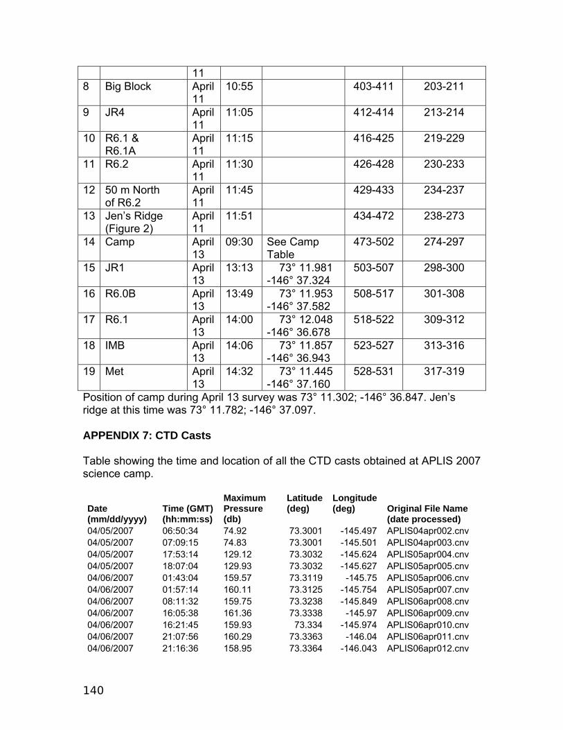
140

11 8 Big Block April

11 10:55 403-411 203-211

9 JR4 April 11

11:05 412-414 213-214

10 R6.1 & R6.1A

April 11

11:15 416-425 219-229

11 R6.2 April 11

11:30 426-428 230-233

12 50 m North of R6.2

April 11

11:45 429-433 234-237

13 Jen’s Ridge (Figure 2)

April 11

11:51 434-472 238-273

14 Camp April 13

09:30 See Camp Table

473-502 274-297

15 JR1 April 13

13:13 73° 11.981 -146° 37.324

503-507 298-300

16 R6.0B April 13

13:49 73° 11.953 -146° 37.582

508-517 301-308

17 R6.1 April 13

14:00 73° 12.048 -146° 36.678

518-522 309-312

18 IMB April 13

14:06 73° 11.857 -146° 36.943

523-527 313-316

19 Met April 13

14:32 73° 11.445 -146° 37.160

528-531 317-319

Position of camp during April 13 survey was 73° 11.302; -146° 36.847. Jen’s ridge at this time was 73° 11.782; -146° 37.097. APPENDIX 7: CTD Casts Table showing the time and location of all the CTD casts obtained at APLIS 2007 science camp.

Date (mm/dd/yyyy)

Time (GMT) (hh:mm:ss)

Maximum Pressure (db)

Latitude(deg)

Longitude(deg) Original File Name

(date processed) 04/05/2007 06:50:34 74.92 73.3001 -145.497 APLIS04apr002.cnv 04/05/2007 07:09:15 74.83 73.3001 -145.501 APLIS04apr003.cnv 04/05/2007 17:53:14 129.12 73.3032 -145.624 APLIS05apr004.cnv 04/05/2007 18:07:04 129.93 73.3032 -145.627 APLIS05apr005.cnv 04/06/2007 01:43:04 159.57 73.3119 -145.75 APLIS05apr006.cnv 04/06/2007 01:57:14 160.11 73.3125 -145.754 APLIS05apr007.cnv 04/06/2007 08:11:32 159.75 73.3238 -145.849 APLIS06apr008.cnv 04/06/2007 16:05:38 161.36 73.3338 -145.97 APLIS06apr009.cnv 04/06/2007 16:21:45 159.93 73.334 -145.974 APLIS06apr010.cnv 04/06/2007 21:07:56 160.29 73.3363 -146.04 APLIS06apr011.cnv 04/06/2007 21:16:36 158.95 73.3364 -146.043 APLIS06apr012.cnv

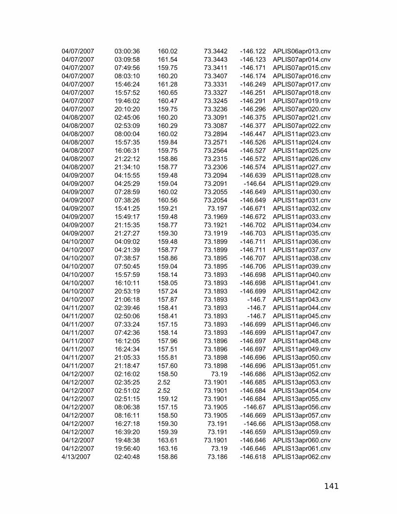
141

04/07/2007 03:00:36 160.02 73.3442 -146.122 APLIS06apr013.cnv 04/07/2007 03:09:58 161.54 73.3443 -146.123 APLIS07apr014.cnv 04/07/2007 07:49:56 159.75 73.3411 -146.171 APLIS07apr015.cnv 04/07/2007 08:03:10 160.20 73.3407 -146.174 APLIS07apr016.cnv 04/07/2007 15:46:24 161.28 73.3331 -146.249 APLIS07apr017.cnv 04/07/2007 15:57:52 160.65 73.3327 -146.251 APLIS07apr018.cnv 04/07/2007 19:46:02 160.47 73.3245 -146.291 APLIS07apr019.cnv 04/07/2007 20:10:20 159.75 73.3236 -146.296 APLIS07apr020.cnv 04/08/2007 02:45:06 160.20 73.3091 -146.375 APLIS07apr021.cnv 04/08/2007 02:53:09 160.29 73.3087 -146.377 APLIS07apr022.cnv 04/08/2007 08:00:04 160.02 73.2894 -146.447 APLIS11apr023.cnv 04/08/2007 15:57:35 159.84 73.2571 -146.526 APLIS11apr024.cnv 04/08/2007 16:06:31 159.75 73.2564 -146.527 APLIS11apr025.cnv 04/08/2007 21:22:12 158.86 73.2315 -146.572 APLIS11apr026.cnv 04/08/2007 21:34:10 158.77 73.2306 -146.574 APLIS11apr027.cnv 04/09/2007 04:15:55 159.48 73.2094 -146.639 APLIS11apr028.cnv 04/09/2007 04:25:29 159.04 73.2091 -146.64 APLIS11apr029.cnv 04/09/2007 07:28:59 160.02 73.2055 -146.649 APLIS11apr030.cnv 04/09/2007 07:38:26 160.56 73.2054 -146.649 APLIS11apr031.cnv 04/09/2007 15:41:25 159.21 73.197 -146.671 APLIS11apr032.cnv 04/09/2007 15:49:17 159.48 73.1969 -146.672 APLIS11apr033.cnv 04/09/2007 21:15:35 158.77 73.1921 -146.702 APLIS11apr034.cnv 04/09/2007 21:27:27 159.30 73.1919 -146.703 APLIS11apr035.cnv 04/10/2007 04:09:02 159.48 73.1899 -146.711 APLIS11apr036.cnv 04/10/2007 04:21:39 158.77 73.1899 -146.711 APLIS11apr037.cnv 04/10/2007 07:38:57 158.86 73.1895 -146.707 APLIS11apr038.cnv 04/10/2007 07:50:45 159.04 73.1895 -146.706 APLIS11apr039.cnv 04/10/2007 15:57:59 158.14 73.1893 -146.698 APLIS11apr040.cnv 04/10/2007 16:10:11 158.05 73.1893 -146.698 APLIS11apr041.cnv 04/10/2007 20:53:19 157.24 73.1893 -146.699 APLIS11apr042.cnv 04/10/2007 21:06:18 157.87 73.1893 -146.7 APLIS11apr043.cnv 04/11/2007 02:39:46 158.41 73.1893 -146.7 APLIS11apr044.cnv 04/11/2007 02:50:06 158.41 73.1893 -146.7 APLIS11apr045.cnv 04/11/2007 07:33:24 157.15 73.1893 -146.699 APLIS11apr046.cnv 04/11/2007 07:42:36 158.14 73.1893 -146.699 APLIS11apr047.cnv 04/11/2007 16:12:05 157.96 73.1896 -146.697 APLIS11apr048.cnv 04/11/2007 16:24:34 157.51 73.1896 -146.697 APLIS11apr049.cnv 04/11/2007 21:05:33 155.81 73.1898 -146.696 APLIS13apr050.cnv 04/11/2007 21:18:47 157.60 73.1898 -146.696 APLIS13apr051.cnv 04/12/2007 02:16:02 158.50 73.19 -146.686 APLIS13apr052.cnv 04/12/2007 02:35:25 2.52 73.1901 -146.685 APLIS13apr053.cnv 04/12/2007 02:51:02 2.52 73.1901 -146.684 APLIS13apr054.cnv 04/12/2007 02:51:15 159.12 73.1901 -146.684 APLIS13apr055.cnv 04/12/2007 08:06:38 157.15 73.1905 -146.67 APLIS13apr056.cnv 04/12/2007 08:16:11 158.50 73.1905 -146.669 APLIS13apr057.cnv 04/12/2007 16:27:18 159.30 73.191 -146.66 APLIS13apr058.cnv 04/12/2007 16:39:20 159.39 73.191 -146.659 APLIS13apr059.cnv 04/12/2007 19:48:38 163.61 73.1901 -146.646 APLIS13apr060.cnv 04/12/2007 19:56:40 163.16 73.19 -146.646 APLIS13apr061.cnv 4/13/2007 02:40:48 158.86 73.186 -146.618 APLIS13apr062.cnv

142

4/13/2007 02:53:56 158.41 73.186 -146.617 APLIS13apr063.cnv 4/13/2007 07:42:11 158.86 73.1863 -146.607 APLIS13apr064.cnv 4/13/2007 07:57:08 157.87 73.1863 -146.607 APLIS13apr065.cnv

143

References Arctic Climate Impact Assesment (ACIA) (2005). Impacts of a warming climate: Arctic climate impact assessment, Hassol, S.J., University of Cambridge Press, 139 pp. Babko, O., D.A. Rothrock, and G.A. Maykut (2002). Role of rafting in the mechanical redistribution of sea ice thickness, J. Geophys. Res., 107(C8), 10.1029/1999JC000190.

Cox, G.F.N. and J.B. Johnson (1983). Stress measurements in ice. USA Cold Regions Research and Engineering Laboratory, CRREL Report 83–23.

Eicken, H., W.B. Tucker III and D.K. Perovich (2001) Indirect measurements of the mass balance of summer Arctic sea ice with an electromagnetic induction technique. Annals of Glaciology, 33: 194-200. Haas, C., S. Gerland, H. Eicken and H. Miller (1997) Comparison of sea-ice thickness measurements under summer and winter conditions in the Arctic using a small electromagnetic induction device. Geophysics, 62(3):749-757. Hibler, W.D., III (1980). Modeling a variabile thickness sea ice cover, Monthly Weather Review, 108, 1943-1973. Hibler, W.D., III (1979). A dynamic-thermodynamic sea ice model, J. Phys. Oc., 9, 815-846. Hutchings, J.K. (2001). On modelling the mass of Arctic sea ice, Ph.D. Thesis, University of London, 153 pp. Kreyscher, M., M. Harder, P. Lemke, and G. Flato (2000). Results of the sea ice model intercomparison project: Evaluation of sea ice rheology shemes for use in climate simulations, J. Geophys. Res.,105(C5), 11,299-11,320. Kwok, R. (2001). Deformation of the Arctic Ocean ice cover between November 1996 and April 1997: A survey. In: IUTAM Symposium on Scaling Laws in Ice Mechanics and Ice Dynamics, Dempsey, J.P. and H.H. Shen (eds.), Kluwer Academic Publishers, 315-323. Laxon, S. W., Peacock, N., and Smith, D. (2003). High Interannual Variability of Sea Ice Thickness in the Arctic Region, Nature, Vol. 425, pp 947-950, doi: 10.1038/nature02050, October 30. Marsden, D., H. Stern, R. Lindsay, and J. Weiss (2004). Scale dependence and localization of the deformation of Arctic sea ice, Phys. Rev. Lett, 93, 17.

144

Overland, J.E., B.A. Walter, T.B. Curtin, and P. Turet (1995). Hierarchy and sea ice mechanics: A case study from the Beaufort Sea, J. Geophys. Res., 100, 4559-4571. Peacock, N. R., and Laxon, S. W. (2004). Sea surface height determination in the Arctic Ocean from ERS altimetry, Journal of Geophysical Research, Vol. 109, C07001, doi:10.1029/2001JC001026. Perovich, D.K., T.C. Grenfell, J.A. Richter-Menge, B. Light, W.B. Tucker, and H. Eicken (2003). Thin and thinner: Sea ice mass balance measurements during SHEBA, J. Geophys. Res., doi: 10.1029/2001JC001079. Pritchard, R.S. (1976). An elastic-plastic constitutive law for sea ice, J. Appl. Mech., 42(2), 379-384. Richter-Menge, J.A. and B.C. Elder (1998). Characteristics of pack ice in the Alaskan Beaufort Sea. Journal of Geophysical Research 103 (C10): 21,817–21,829.

Richter-Menge, J., B. Elder, K. Claffey, J. Overland and S. Salo (2002). In situ sea ice stresses in the western arctic during the winter of 2001-2002. Proceedings of the 16 th IAHR International Symposium on Ice, New Zealand, 2-6 December 2002, International Association of Hydraulic Engineering and Research, 131-138.

Richter-Menge, J.A, D.K. Perovich, B.C. Elder, K. Calffey, I. Rigor and M. Ortmeyer (2006) Ice Mass Balance Buoys: A tool for measuring and attributing changes in the thickness of the Arctic sea ice cover, Annals of Glaciol., 44: 205-210.

Richter-Menge, J. A., S. L. McNutt, J. E. Overland, and R. Kwok (2002) Relating arctic pack ice stress and deformation under winter conditions, J ournal of Geophysical Research , 107(C10), 8040.

Roberts, A. (2005). Medium-range numerical prediction of Antarctic sea ice, Postgraduate University of Hobart, Tasmania, Australia, 220 pp. Rothrock, D.A. (1975). The energetics of the plastic deformation of pack ice by ridging, J. Geophys. Res., 80(33), 4514-4519. Schneider, W. and G. Budéus (1997). A note on Norske Ø Ice Barrier (Northeast Greenland, viewed by Landsat 5 TM. J. Mar. Sys., 10, 99-106. Schulson, E.M. and W.D. Hibler, III (2004). Fracture of the winter sea ice cover of the Arctic Ocean, J. Geophys. Res.,109, B09207, 10 pp.

145

Steele, M. and G.M. Flato (1999). Sea ice growth, melt, and modeling: A survey. In: The Arctic Ocean Freshwater Budget, NATO ARW, 70, 549-587. Sturm, M. and J. Holmgren (1999) Self-recording snow depth probe. U.S. Patent 5,864,059. (Assigned to U.S. Army Corps of Engineers, Cold Regions Research and Engineering Laboratory) Trembley, L.B. and L.A. Mysak (1997). Modeling sea ice as a granular plastic, including the dilatancy effect, J. Phys. Oc., 27(11), 2342-2360.