Embed Size (px)
Citation preview
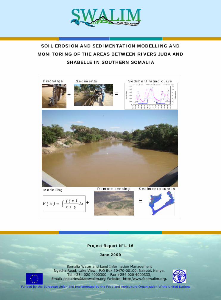
SOIL EROSION AND SEDIMENTATION MODELLING AND
MONITORING OF THE AREAS BETWEEN RIVERS JUBA AND
SHABELLE IN SOUTHERN SOMALIA
Project Report N°L-16
June 2009
Somalia Water and Land Information Management Ngecha Road, Lake View. P.O Box 30470-00100, Nairobi, Kenya.
Tel +254 020 4000300 - Fax +254 020 4000333, Email: [email protected] Website: http//www.faoswalim.org.
Funded by the European Union and implemented by the Food and Agriculture Organization of the United Nations
0
2 0 0 0
4 0 0 0
6 0 0 0
8 0 0 0
1 0 0 0 0
1 2 0 0 0
Nov
-89
Dec
-89
Jan-
90
Feb-
90
Mar
-90
Apr
-90
May
-90
Jun-
90
Jul-9
0
Aug
-90
Sep-
90
Oct
-90
Nov
-90
Dec
-90
Sed.
Con
c. (p
pm)
0
2 0
4 0
6 0
8 0
1 0 0
1 2 0
Disc
harg
e (m
3/s)
S e d . C o n c . ra in fa l l se a s o n D is c h a r g e
D is c h a rg e S e d im e n ts
+ =
∫ += d x
yx)x(f)x(F + =
M o d e llin g R e m o te s e n s in g S e d im e n t s o u rc e s
S e d im e n t ra t in g c u rv e

ii
Disclaimer
The designations employed and the presentation of material in this information product
do not imply the express opinion whatsoever on the part of the Food and Agriculture
Organization of the United Nations concerning the legal status of any country, territory,
city or area or of its authorities, or concerning the delimitation of its frontiers or
boundaries.
This document should be cited as follows:
FA0-SWALIM Technical Report No. L-16: Omuto, C.T., Vargas, R. R., Paron, P. 2009. Soil
erosion and sedimentation modelling and monitoring framework of the areas between
rivers Juba and Shabelle in southern Somalia. Nairobi, Kenya.

iii
Acknowledgements
We wish to acknowledge the considerable support and guidance given by FAO-
SWALIM’s CTA Dr. Zoltan Balint.
A special acknowledge also goes to all field officers who collected the samples used
in this study.
The XRD analysis could not have been performed without the support of Prof. Ciriaco
Giampaolo of the Department of Geological Sciences of University Roma TRE, in
Rome, Italy. We do appreciate the support given.
Finally we express our acknowledgment to all FAO-SWALIM staff for their input
during data collection and analysis.
iv
Table of contents
Disclaimer....................................................................................................ii
Acknowledgements ..................................................................................... iii
List of figure ...............................................................................................vi
List of tables ............................................................................................. viii
List of acronyms..........................................................................................ix
1. INTRODUCTION................................................................................. 1
1.1 Background ..................................................................................... 1
1.2 Definition of terms associated with soil erosion and sedimentation ........... 2
1.2.1 Soil erosion................................................................................... 2
1.2.2 Sedimentation............................................................................... 4
1.3 Modelling of soil erosion and sediment flux ........................................... 5
1.4 Approach for preliminary study of soil erosion and sedimentation study in
south Somalia ................................................................................... 8
2. STUDY AREA.....................................................................................11
2.1 Rainfall distribution ..........................................................................11
2.2 Geology and soil ..............................................................................12
2.3 Land cover and land use ...................................................................14
3. MATERIALS AND METHODS ..............................................................15
3.1 Data sources...................................................................................15
3.1.1 Sediment sampling and river discharge measurements ......................15
3.1.2 Other datasets .............................................................................20
3.2. X-Ray Diffractometry (XRD)..............................................................21
v
3.3 Soil erosion modelling and estimation of sediment yields .......................24
4. RESULTS AND DISCUSSIONS ............................................................28
4.1 Modelling of topsoil loss ....................................................................28
4.2 Comparison of modelling and rating curve estimates of sediment yield ....30
4.3 X-Ray diffractometry ........................................................................33
4.4 Potential sites for monitoring sediments ..............................................36
5. RECOMMENDATIONS FOR MONITORING EROSION AND
SEDIMENTATION IN SOUTH SOMALIA ............................................38
5.1 Theoretical framework for monitoring soil erosion and sedimentation ......38
5.1.1 Monitoring soil erosion ..................................................................39
5.1.2 Monitoring sediment sources ..........................................................42
5.1.3 Monitoring suspended sediment discharge........................................44
5.2 Practical steps towards monitoring soil erosion and sedimentation in south
Somalia...........................................................................................46
6. CONCLUSIONS AND RECOMMENDATIONS ..........................................48
6.1 Conclusions ....................................................................................48
6.1.1 Potential sources of sediments........................................................48
6.1.2 Techniques and opportunities for monitoring sediments yields.............48
6.2 Recommendations ...........................................................................48
REFERENCES ..............................................................................................51
APPENDICES ..............................................................................................54
Appendix 1: Input data preparation for soil erosion modelling...........................54
Appendix 2: Mineral glossary .......................................................................59
vi
List of figures
Figure 1.1: Schematic view of soil erosion types in a basin................................... 3
Figure 1.2: Typical hysteresis effect observable in suspended sediments................ 7
Figure 1.3: Approach for preliminary study of soil erosion and sedimentation.......... 9
Figure 2.1: Study area...................................................................................11
Figure 2.2: Soil map of the study area .............................................................13
Figure 3.1: Sampler for sediment sampling.......................................................15
Figure 3.2: Location of sediment and river discharge measurements in 2007 and
2008 ...........................................................................................16
Figure 3.3: Sediment and river discharge sampling in Jowhar, south Somalia ........17
Figure 3.4: Example of laboratory report of analysis of sediment sample from Johwar
sampling station............................................................................18
Figure 3.5: Example of sediment and discharge patterns in Belet Wyne in 2008 .....19
Figure 3.6: Average monthly rainfall for 19 stations in the study area in 2008 .......20
Figure 3.7: Location of soil samples and summary of soil physical properties .........21
Figure 3.8: Electromagnetic spectrum and X-Ray window. ..................................23
Figure 3.9: X-Ray diffractometer and the goniometer principle. T is transmitter of X-
Ray and C is cathode detector .........................................................23
Figure 3.10: A typical X-ray Diffractogram........................................................24
Figure 3.11: Sediment rating curve for river Juba and Shabelle in Somalia ............27
Figure 4.1: Example of MUSLE topsoil loss estimate in 2007 and 2008..................29
Figure 4.2: Comparison of sediment yield by rating curve and MUSLE model .........32
Figure 4.3: spectra of XRD from the samples of Belet Weyne and Buale. ...............33
Figure 4.4: Simplified geologic map of the Juba and Shabelle watershed. ..............35
Figure 4.5: Potential sediments sources and monitoring sites in the study area......37
Figure 4.6: Landscape cross-section from river Shabelle to the Indian Ocean near
Mogadishu....................................................................................38

vii
Figure 5.1: Theoretical framework for soil erosion and sedimentation monitoring in
south Somalia ...............................................................................39
Figure 5.2: Field-measurement method for monitoring soil erosion.......................41
Figure 5.3: Framework for spatial monitoring of soil erosion................................42
Figure 5.4: Soil-sample collection from the field ................................................43
Figure 5.5: River gauging stations in the study area...........................................45
Figure 5.6: Field sampling for periodic monitoring of sediment flux.......................46
viii
List of tables
Table 1.1: Soil erosion model selection.............................................................. 5
Table 3.1: River discharge for river Juba and Shabelle in 2007 and 2008 ..............18
Table 3.2: Models for estimating overland sediment yield ...................................25
Table 3.3: Summary of sediment concentration in 2007 and 2008 .......................26
Table 4.1: Soil loss estimates between sediment measuring stations ....................28
Table 4.2: Sediment yield from the rating curve compared with modelling.............30
Table 5.1: Practical steps towards monitoring soil erosion and sedimentation in south
Somalia .......................................................................................47
Table 5.2: Potential requirements for implementing soil erosion and sedimentation
monitoring framework....................................................................47
Table A.1: Guidelines for determining runoff curve numbers................................55

ix
List of acronyms
CN - Curve Number
CTA - Chief Technical Advisor
FAO - Food and Agriculture Organisation
ITCZ - Inter-Tropical Convergence Zone
MODIS - Moderate Resolution Imaging Spectrometer
MUSLE - Modified Universal Soil Loss Equation
PVC - Polyvinyl Chloride
RUSLE - Revised Universal Soil Loss Equation
SDR - Sediment Delivery Ratio
SCS - Soil Conservation Service
SSC - Suspended Sediment Concentration
SWALIM - Somalia Water and Land Information Management
TSS - Total Suspended Solids
XRD - X-Ray Diffractometry
1
1. INTRODUCTION
1.1 Background
Soil erosion is a complex dynamic process by which the productive soil surface is
detached, transported, and accumulated at a distant place. It produces exposed sub-
surface where the soil has been detached and the detached deposited in low-lying
areas of the landscape or in water bodies downstream in a process known as
sedimentation. Soil erosion and sedimentation are concurring environmental
processes with varied negative and positive impacts. The negative impacts include
the removal of nutrient rich topsoil in upland areas and subsequent reduction of
agricultural productivity in those areas. In irrigation projects, soil erosion and
sedimentation cause reduction of irrigation conveyance capacities and reservoir
storage volumes. They also reduce irrigation water quality by increasing water
turbidity. In the lowlands, deposition of soil from eroded uplands causes changes in
river channels and subsequent increase in flood vulnerability of the floodplain
farmlands and residential areas.
Soil erosion and sedimentation is not also always a negative environmental process.
Whenever soil erosion occurs, there may be downstream benefits such as deposition
of rich sediments for promotion of agricultural activities. Examples include Nile basin
irrigation systems in Egypt, Juba and Shabelle irrigation projects in Somalia, etc.
In south Somalia, rivers Juba and Shabelle are the main rivers supplying irrigation
water for many agricultural activities in the region. However, over many years and
more specifically in the last 20 years, the irrigation projects have experienced high
sediment loads which hamper their operation. Upland soil erosion is believed to be
the major cause for this high sediment load [11]. Generally, upland areas with high
soil erosion rates tend to contribute more sediment compared to areas with low soil
erosion rates. In order to reduce the sediment plume into the two rivers, contributing
areas with high soil erosion rates need to be identified and targeted for soil erosion
control measures. Many Somalia development partners are currently putting special
attention towards rehabilitating irrigation schemes in south Somalia and even initiate
soil erosion control in the upland areas. However, this desire and anticipated
initiative lack sufficient information on soil erosion and sedimentation rates, potential
sediment sources, and sediment flow-rate in the two rivers.
2
The present study by FAO-SWALIM was initiated with the general objective of
preparing an assessment of soil erosion and sedimentation of the riverine areas
between rivers Juba and Shabelle and to provide input into soil erosion-
sedimentation monitoring framework which will contribute to improved management
of the irrigation systems in south Somalia. The study identified areas prone to high
soil erosion rates and sediment flux into river Juba and Shabelle in south Somalia. It
also proposed a comprehensive monitoring framework which will support routine
identification of soil erosion and sedimentation problems for quick and targeted
interventions. The methods and main findings of this study are documented in
technical report.
1.2 Definition of terms associated with soil erosion and sedimentation
1.2.1 Soil erosion
Soil erosion may be defined as detachment, transportation, and deposition of soil
particles from one place to another under the influence of wind, water or
gravitational forces. In broad sense, soil erosion process can be classified into two
categories: geologic and accelerated erosion. Geologic erosion refers to the
simultaneous formation and loss of soil which maintain the balance between soil
forming processes and soil loss. It is a natural process. Accelerated erosion includes
deterioration and loss of soil by human activities. It is called “accelerated” because it
speeds up the geologic soil erosion; thus upsetting the balance between soil forming
processes and soil loss. Accelerated soil erosion occurs in various forms (e.g. splash,
sheet, rill, and gullies) depending on the stage of progress in the erosion cycle and
the position in the landscape. Some types of accelerated erosion may be used to
refer to where the erosion process occurs (e.g. trail erosion, riverbank/riverbed
erosion, road slope erosion, cropland erosion).
The main factors influencing soil erosion include climate (rainfall/precipitation or
wind), landscape relief, soil and bedrock properties, vegetation cover, and human
activity [7, 22]. Of these factors, the climate has been used to further define other
forms of soil erosion such as erosion by wind, raindrop, wind etc. Erosion by rainfall
is induced by when raindrops strike the surface and overcome the forces holding soil
particle together. This is commonly referred to as “rain splash” or “raindrop splash”
3
[27]. As the rainfall process continue, water infiltrates into the soil at a rate
controlled by the intensity of the water hitting the surface and the infiltration
capacity of the vertical soil profile. Water that does not infiltrate begins to pond on
the surface and then flows along the steepest descent after achieving a sufficient
ponding depth. This hydrological process is referred to as “overland flow” or “runoff”
[22]. In the upland areas of a landscape, overland flow is conceptually divided into
rill flow and inter-rill flow mechanisms. As overland flow converges from various
portions of the upland area and becomes more concentrated, it becomes sufficiently
erosive to form shallow channels, referred to as “rills” (Figure 1.1). Additional soil
particles may become detached as water flows through these rills. In the inter-rill
areas, runoff may occur as a very thin broad sheet, sometimes referred to as “sheet
flow”. Both detachment and transport may occur in the rill and inter-rill areas. As
erosive power increases, the small rills converge to form a large and deep surface
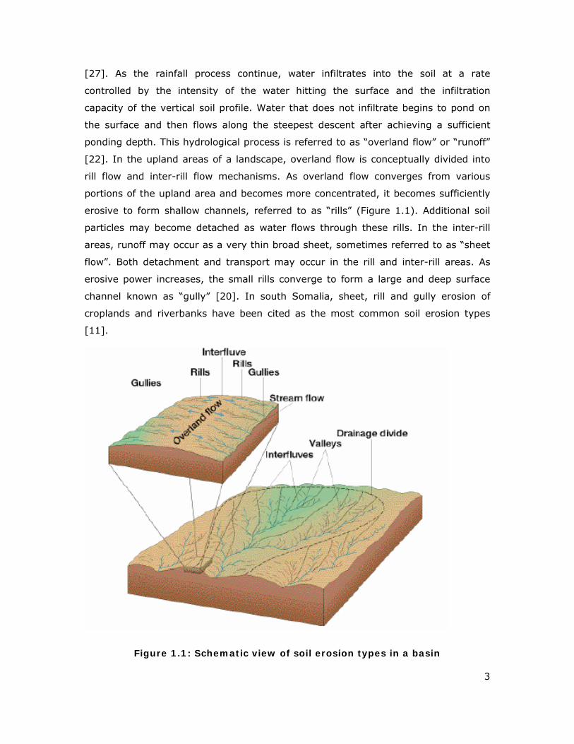
channel known as “gully” [20]. In south Somalia, sheet, rill and gully erosion of
croplands and riverbanks have been cited as the most common soil erosion types
[11].
Figure 1.1: Schematic view of soil erosion types in a basin
4
1.2.2 Sedimentation
The entrained soil materials carried in water or air is known as sediment. The main
sources of sediments are soil erosion of upland areas or river channel, mass
movement due to landslides, soil creeps etc, and from mining or dumps lefts as
waste material. In south Somalia, soil erosion is the major source of sediments into
rivers Juba and Shabelle.
Sediment transport is a direct function of water or wind movement. With respect to
water movement in a river, during sediment transport, sediment particles become
separated into three categories: suspended material which includes silt + clay +
sand; the coarser, relatively inactive bedload and the saltation load. Suspended load
comprises sand + silt + clay-sized particles that are held in suspension because of
the turbulence of the water. The suspended load is further divided into the wash load
which is generally considered to be the silt + clay-sized material (< 62 µm in particle
diameter) and is often referred to as “fine-grained sediment”. The wash load is
mainly controlled by the supply of this material (usually by means of erosion). The
amount of sand (>62 µm in particle size) in the suspended load is directly
proportional to the turbulence and mainly originates from erosion of the bed and
banks of the river. In many rivers, suspended sediment (i.e. the mineral fraction)
forms most of the transported load. Bedload is stony material, such as gravel and
cobbles that moves by rolling along the bed of a river because it is too heavy to be
lifted into suspension by the current of the river. Bedload is especially important
during periods of extremely high discharge and in landscapes of large topographical
relief, where the river gradient is steep (such as in mountains). It is rarely important
in low-lying areas such as lower parts of river Juba and Shabelle in south Somalia.
Saltation load is a term used by sedimentologists to describe material that is
transitional between bedload and suspended load. Saltation means “bouncing” and
refers to particles that are light enough to be picked off the river bed by turbulence
but too heavy to remain in suspension and, therefore, sink back to the river bed.
Saltation load is never measured in operational hydrology [10, 22].
Sediment transport is facilitated when there is sufficient energy to carry the
sediments. The mass rate of transport is known as “sediment discharge”. If at any
point during the transport the velocity of the water is reduced, some sediment will be
deposited. The process is known as sedimentation. Sediment yield is the amount of
eroded soil that is delivered to a point in the catchment [22].
5
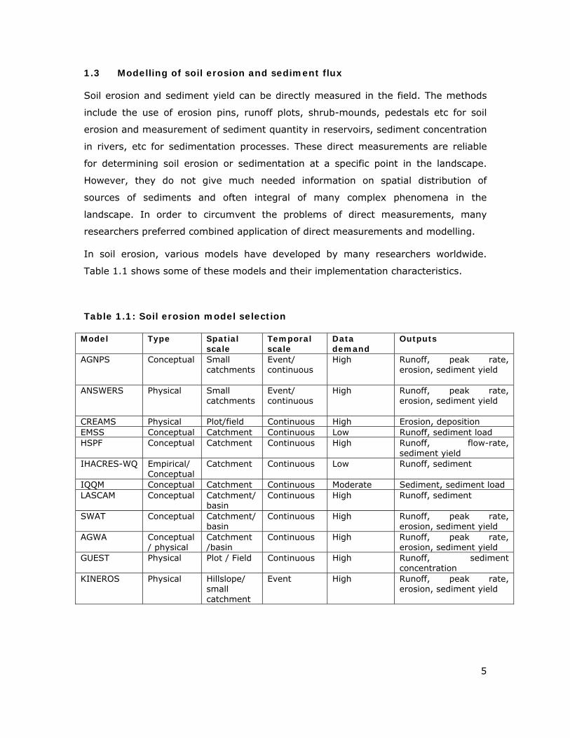
1.3 Modelling of soil erosion and sediment flux
Soil erosion and sediment yield can be directly measured in the field. The methods
include the use of erosion pins, runoff plots, shrub-mounds, pedestals etc for soil
erosion and measurement of sediment quantity in reservoirs, sediment concentration
in rivers, etc for sedimentation processes. These direct measurements are reliable
for determining soil erosion or sedimentation at a specific point in the landscape.
However, they do not give much needed information on spatial distribution of
sources of sediments and often integral of many complex phenomena in the
landscape. In order to circumvent the problems of direct measurements, many
researchers preferred combined application of direct measurements and modelling.
In soil erosion, various models have developed by many researchers worldwide.
Table 1.1 shows some of these models and their implementation characteristics.
Table 1.1: Soil erosion model selection
Model Type Spatial scale
Temporal scale
Data demand
Outputs
AGNPS Conceptual Small catchments
Event/ continuous
High Runoff, peak rate, erosion, sediment yield
ANSWERS Physical Small catchments
Event/ continuous
High Runoff, peak rate, erosion, sediment yield
CREAMS Physical Plot/field Continuous High Erosion, deposition EMSS Conceptual Catchment Continuous Low Runoff, sediment load HSPF Conceptual Catchment Continuous High Runoff, flow-rate,
sediment yield IHACRES-WQ Empirical/
Conceptual Catchment Continuous Low Runoff, sediment
IQQM Conceptual Catchment Continuous Moderate Sediment, sediment load LASCAM Conceptual Catchment/
basin Continuous High Runoff, sediment
SWAT Conceptual Catchment/ basin
Continuous High Runoff, peak rate, erosion, sediment yield
AGWA Conceptual/ physical
Catchment /basin
Continuous High Runoff, peak rate, erosion, sediment yield
GUEST Physical Plot / Field Continuous High Runoff, sediment concentration
KINEROS Physical Hillslope/ small catchment
Event High Runoff, peak rate, erosion, sediment yield
6
Table 1.1 Cont.
Model Type Spatial scale
Temporal scale
Data demand
Outputs
LISEM Physical Small catchment
Event High Runoff, sediment
EUROSEM Physical Small catchment
Event High Runoff, erosion, sediment
TOPOG Physical Hillslope High Erosion hazard USLE Empirical Hillslope Annual Low Erosion RUSLE Empirical Hillslope Annual Low Erosion USPED Empirical/
conceptual Catchment Event/
annual Moderate Erosion, deposition
Thornes Conceptual/ empirical
Hillslope/ catchment
Event Moderate Runoff, erosion
WATEM Conceptual Catchment Annual Moderate Erosion WEPP Physical Hillslope/
catchment Continuous High Runoff, sediment yield,
soil loss SHETRAN Physical Catchment Event High Runoff, peak rate,
erosion, sediment yield SEAGIS Empirical/
conceptual Catchment Annual High Erosion, sediment yield
PESERA Physical Hillslope Continuous High Runoff, erosion, sediment SPL Empirical/
conceptual Catchment/ river basin
Annual Moderate Fluvial erosion, river incision
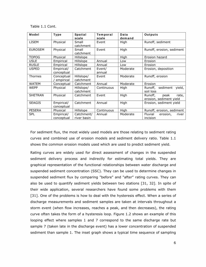
For sediment flux, the most widely used models are those relating to sediment rating
curves and combined use of erosion models and sediment delivery ratio. Table 1.1
shows the common erosion models used which are used to predict sediment yield.
Rating curves are widely used for direct assessment of changes in the suspended
sediment delivery process and indirectly for estimating total yields. They are
graphical representation of the functional relationships between water discharge and
suspended sediment concentration (SSC). They can be used to determine changes in
suspended sediment flux by comparing "before" and "after" rating curves. They can
also be used to quantify sediment yields between two stations [31, 32]. In spite of
their wide application, several researchers have found some problems with them
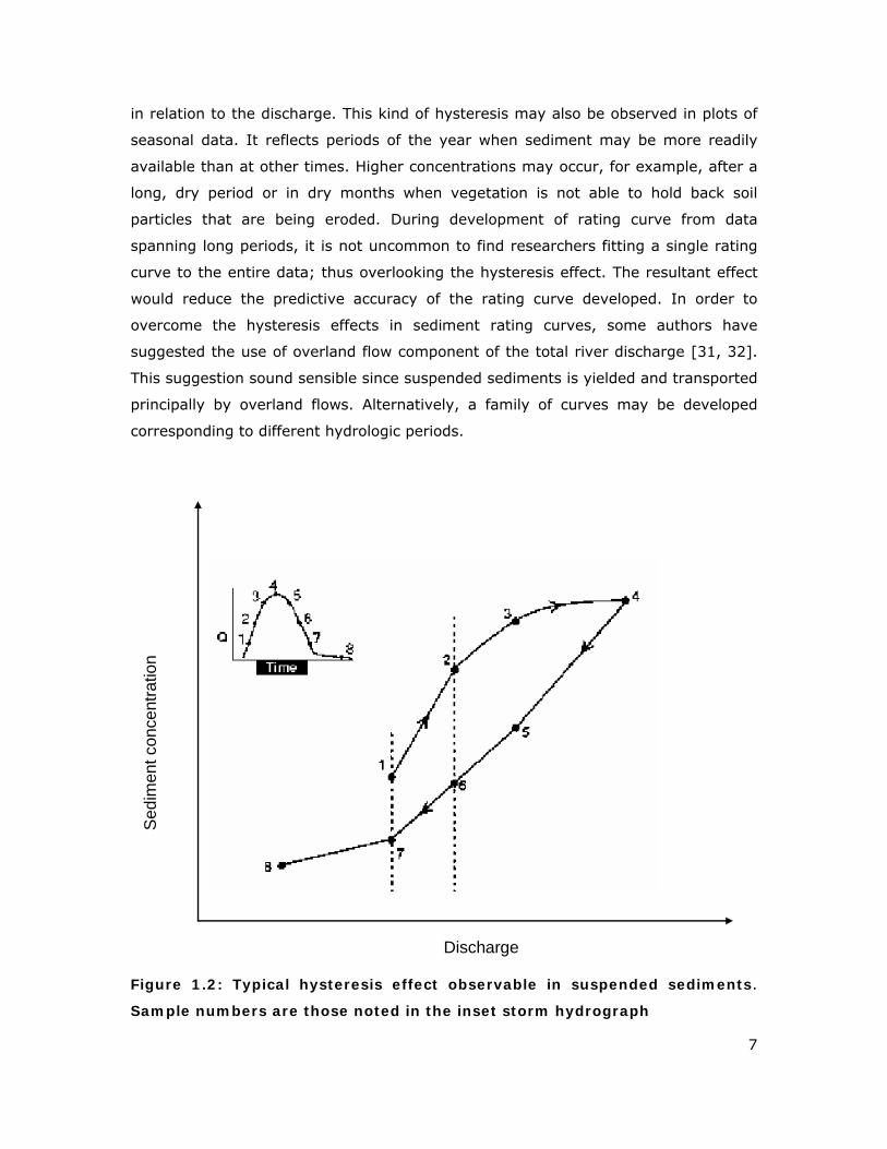
[31]. One of the problems is how to deal with the hysteresis effect. When a series of
discharge measurements and sediment samples are taken at intervals throughout a
storm event (when flow increases, reaches a peak, and then decreases), the rating
curve often takes the form of a hysteresis loop. Figure 1.2 shows an example of this
looping effect where samples 1 and 7 correspond to the same discharge rate but
sample 7 (taken late in the discharge event) has a lower concentration of suspended
sediment than sample 1. The inset graph shows a typical time sequence of sampling
7
in relation to the discharge. This kind of hysteresis may also be observed in plots of
seasonal data. It reflects periods of the year when sediment may be more readily
available than at other times. Higher concentrations may occur, for example, after a
long, dry period or in dry months when vegetation is not able to hold back soil
particles that are being eroded. During development of rating curve from data
spanning long periods, it is not uncommon to find researchers fitting a single rating
curve to the entire data; thus overlooking the hysteresis effect. The resultant effect
would reduce the predictive accuracy of the rating curve developed. In order to
overcome the hysteresis effects in sediment rating curves, some authors have
suggested the use of overland flow component of the total river discharge [31, 32].
This suggestion sound sensible since suspended sediments is yielded and transported
principally by overland flows. Alternatively, a family of curves may be developed
corresponding to different hydrologic periods.
Sed
imen
t con
cent
ratio
n
Discharge
Figure 1.2: Typical hysteresis effect observable in suspended sediments.
Sample numbers are those noted in the inset storm hydrograph
8
1.4 Approach for preliminary study of soil erosion and sedimentation
study in south Somalia
Due to the current fragile security situation in southern Somalia which prevented
detailed field survey, this study basically focused on desk analysis of soil erosion and
sedimentation of the riverine areas along rivers Juba and Shabelle. In addition to
lack of field survey, there was also the lack of comprehensive and consistent
historical data on sediment concentration of the two rivers. Because of these
limitations, this study focused on what could be feasible in designing a monitoring
framework for soil erosion and sedimentation into river Juba and Shabelle. Its main
thrust was therefore to use the available information in developing a versatile
method for assessing soil erosion and sedimentation rates into river Juba and
Shabelle in south Somalia. It also developed a framework for obtaining future
comprehensive data for guiding decisions on river basin management of rivers Juba
and Shabelle. In effect, the study was an input for designing future monitoring of soil
erosion and sedimentation into the two rivers. Its results should therefore be seen
within this context.
The major inputs for the study were remote sensing and archived data at FAO-
SWALIM, on the one hand for erosion, and limited sediment samples and river
discharge in 2007 and 2008, on the other hand for sedimentation (Figure 1.2). The
approach used included three steps: soil erosion modelling, prediction of sediment
flux, and determination of potential monitoring sites and framework for soil erosion
and sedimentation (Figure 1.3).
9
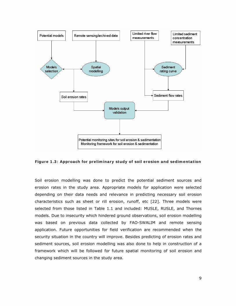
Figure 1.3: Approach for preliminary study of soil erosion and sedimentation
Soil erosion modelling was done to predict the potential sediment sources and
erosion rates in the study area. Appropriate models for application were selected
depending on their data needs and relevance in predicting necessary soil erosion
characteristics such as sheet or rill erosion, runoff, etc [22]. Three models were
selected from those listed in Table 1.1 and included: MUSLE, RUSLE, and Thornes
models. Due to insecurity which hindered ground observations, soil erosion modelling
was based on previous data collected by FAO-SWALIM and remote sensing
application. Future opportunities for field verification are recommended when the
security situation in the country will improve. Besides predicting of erosion rates and
sediment sources, soil erosion modelling was also done to help in construction of a
framework which will be followed for future spatial monitoring of soil erosion and
changing sediment sources in the study area.
10
Sediment flux was predicted using sediment rating curve. The rating curve method
was adopted due to lack of continuous sediment sampling of river Juba and Shabelle
in the study area. The discrete temporal measurements of sediment concentrations
were calibrated with daily measurements of river discharge and the resultant
relationship used to determine annual sediment flux into the two rivers. This
approach was successfully used in this study was to: 1) support the formulation of a
framework for assessing and future monitoring of potential sediment flux into the
two rivers, 2) give insight into the best soil erosion model for predicting sediment
flux in the study area. It is important to note that the focus on the use of sediment
rating curves was not to get decimal digits of accuracy but rather to give insight into
appropriate monitoring methods and potential rates of sedimentation in rivers Juba
and Shabelle in south Somalia.
11
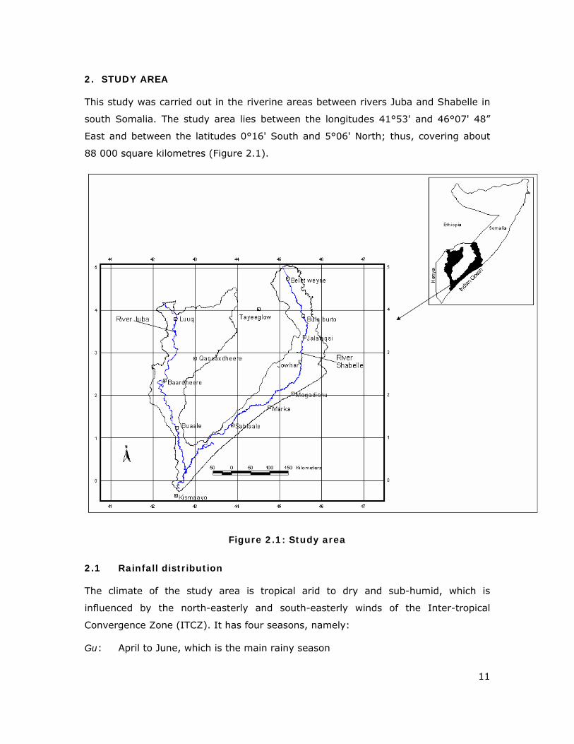
2. STUDY AREA
This study was carried out in the riverine areas between rivers Juba and Shabelle in
south Somalia. The study area lies between the longitudes 41°53' and 46°07' 48”
East and between the latitudes 0°16' South and 5°06' North; thus, covering about
88 000 square kilometres (Figure 2.1).
Figure 2.1: Study area
2.1 Rainfall distribution
The climate of the study area is tropical arid to dry and sub-humid, which is
influenced by the north-easterly and south-easterly winds of the Inter-tropical
Convergence Zone (ITCZ). It has four seasons, namely:
Gu: April to June, which is the main rainy season
12
Xagaa: July to September, which is dry and cool
Deyr: October to December, which is second rainy season
Jilaal: January to March, which is the longest dry season
Rainfall in the study area is erratic, with a bimodal pattern except in the southern
parts close to the Indian Ocean where some showers may occur even during the
Xagaa. Rainfall varies considerably, with the Gu delivering about 60% of the total
mean annual rainfall, which ranges from 200 - 400 mm in areas bordering Ethiopia,
between 400 - 500 mm in the central areas, and above 500 in the southern areas.
2.2 Geology and soil
The study area is characterized by outcropping of the metamorphic basement
complex, which are made up of migmatites and granites. Sedimentary rocks such as
limestones, sandstones, and gypsiferous limestones are also present, as well as an
extensive and wide system of coastal sand dunes. Basaltic flows are present in the
north-western part of the study area. From a tectonic point of view, the study area is
characterized by a fault system lying parallel to the coast and by a system of
northwest-southeast oriented faults in the metamorphic basement complex.
Some late tertiary fluvio-lagunal deposits also occur on the Lower Juba floodplain
and part of the southern Shabelle. This latter part consists of clay, sandy clay, sand,
silt and gravel. Recent fluvial deposits are common alongside the two rivers and
mainly consisting of sand, gravel, clay and sandy clay. Other recent alluvial deposits
in small valleys can be found here. They mainly consist of gravely sand or red sandy
loam materials. A wide coastal dune system also occurs along the coast of Indian
Ocean.
In terms of the landscape features, the study area can be characterized as follows:
• The two main river valleys (river Juba and Shabelle) that traverse the area.
• Hilly topography in the middle of the study area, which is cut by wadis flowing
towards the Indian Ocean.
• A coastal dune complex known as the Marka red dunes, which fringes the
coast from beyond the Kenyan border and separating the narrow coastal plain
from the Webi Shebeli alluvial plain [3].
13
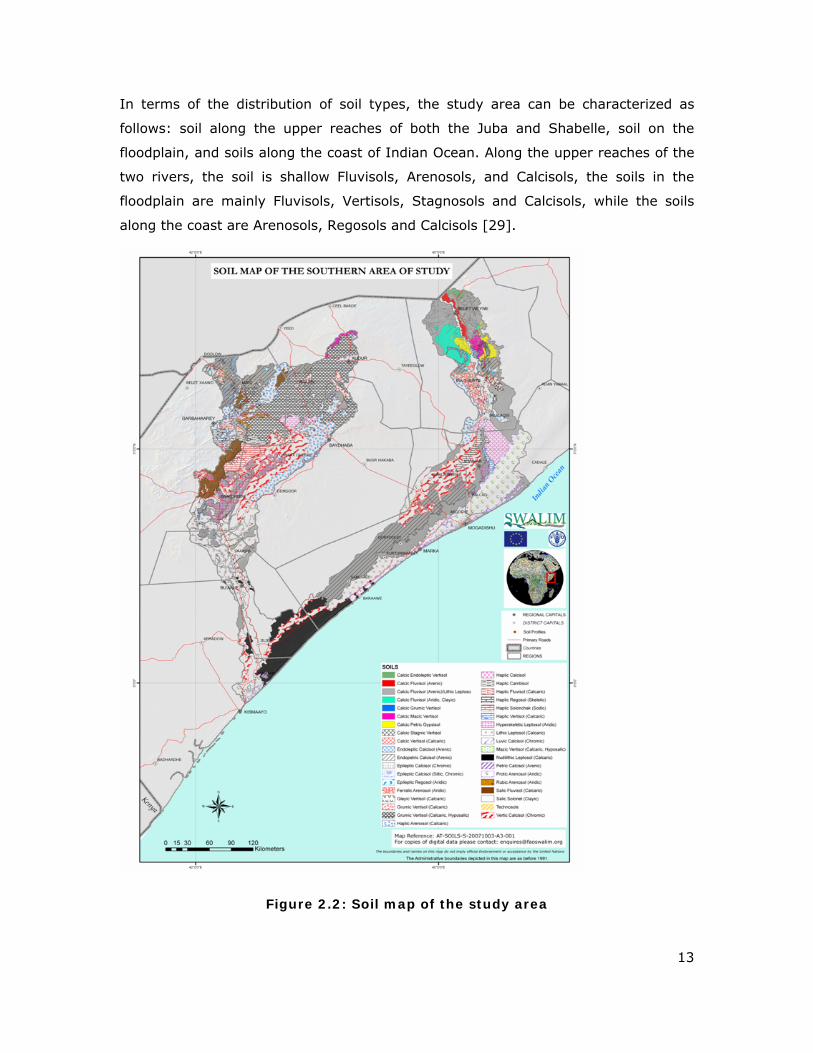
In terms of the distribution of soil types, the study area can be characterized as
follows: soil along the upper reaches of both the Juba and Shabelle, soil on the
floodplain, and soils along the coast of Indian Ocean. Along the upper reaches of the
two rivers, the soil is shallow Fluvisols, Arenosols, and Calcisols, the soils in the
floodplain are mainly Fluvisols, Vertisols, Stagnosols and Calcisols, while the soils
along the coast are Arenosols, Regosols and Calcisols [29].
Figure 2.2: Soil map of the study area
14
2.3 Land cover and land use
Land cover of the study area consists mainly of natural vegetation. Other cover types
include crop fields (both rainfed and irrigated), built-up areas (settlement/towns and
airport), sand dunes and bare lands, and natural water bodies. The natural
vegetation consists of riparian forest, bush lands and grasslands, and woody
vegetation. Woody and herbaceous species include Acacia bussei, A. seyal, A.
nilotica, A. tortilis, A. senegal, Commiphora spp., Chrysopogon auchieri var.
quinqueplumis, Suaeda fruticosa and Salsola foetida etc.
The land use is mainly of grazing and wood collection for fuelwood and building
material. Rangelands in the Juba and Shabelle catchments support livestock such as
goats, sheep, cattle and camels. Livestock ownership is private but grazing lands
have been traditionally communal, making it difficult to regulate the use of
rangeland. Rangelands are utilised by herders using transhumance strategies [1].
Land covers associated with this land use include forest, wooded bushland,
bushlands, shrubland and grasslands [12].
Most farmers in the study area are sedentary who practice animal husbandry in
conjunction with crop production. They tend to keep lactating cattle and a few sheep
and goats near their homes while non-lactating animals are kept further away in
nomadic life pattern. Along the rivers, there are rainfed and irrigation farms where
there are farmers who also keep relatively small numbers of livestock (mainly cattle
and small ruminants). Small-scale irrigated fields (some with pumps and some by
gravity) are also found along the Shabelle and Juba river valleys. Crops grown
include maize, sesame, fruit trees and vegetables. Large-scale plantations sugar
cane, bananas were originally found in these areas prior to the civil war in 1990s.
These plantations have since collapsed during the civil war. However, remnant large-
scale production of guava, lemon, mango and papaya may be spotted in a few
places. Flood recession cultivation in desheks (natural depressions) on the Juba River
floodplain is common. Crops grown include sesame, maize, sesame, tobacco, beans,
peas and vegetables, watermelon, sometime groundnuts.
15
3. MATERIALS AND METHODS
3.1 Data sources
The data used in this study included daily rainfall amounts for 2007 and 2008,
sediment concentration (Total Suspended Sediment, TSS) samples for some stations
in river Juba and Shabelle for certain periods in 2007 and 2008, and daily river flow
measurements at four stations in 2007 and 2008.
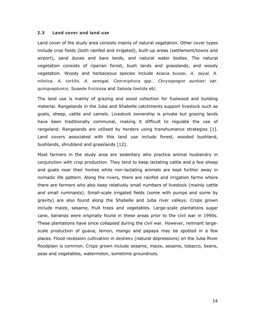
3.1.1 Sediment sampling and river discharge measurements
Sediment samples were collected using instantaneous sampling method. In this
method, a sampler consisting of a horizontal tube with water-tight doors (Figure 3.1)
was lowered into the river. The doors were then opened by triggering an opening
mechanism using suspension cords to allow sediments and water to enter the
sampling bottle (Figure 3.1). The doors were held open long enough for the flow
within the tube to become equal with that outside the tube. They were then suddenly
shut to trap the sediment suspensions inside the bottle.
Sampling bottle
Suspension cord
Nozzle
Horizontal tube
Figure 3.1: Sampler for sediment sampling
16
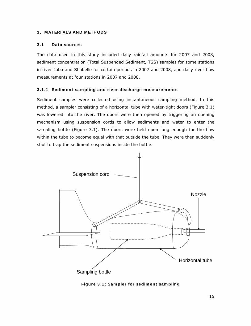
Sediment sampling was done in seven locations (Figure 3.2). Three of these
locations had river gauging equipment for measuring water discharge. Collection of
sediment was done by lowering the sample into the river from the same spot as for
river flow-gauge (Figure 3.3).
#
#
#
#
#
#
S
S
S
S
Luuq
Baardheere
Bu'ale
Audegle
Afgooye
Jowhar
Bulo burti
Belet weyne
River Juba
River Shabelle
Indian Oce
an
50 0 50 100 Kilometers
N
# Sediment sampling locationS River flow measurement location
0°30'30" 0°30'30"
2°1'00" 2°1'00"
3°31'30" 3°31'30"
5°2'00" 5°2'00"
42 °30'30"
42 °30'30"
44°1'00"
44°1'00"
45°31'30"
45°31'30"42
42
43
43
44
44
45
45
46
46
0 0
1 1
2 2
3 3
4 4
5 5
Figure 3.2: Location of sediment and river discharge measurements in 2007
and 2008
17
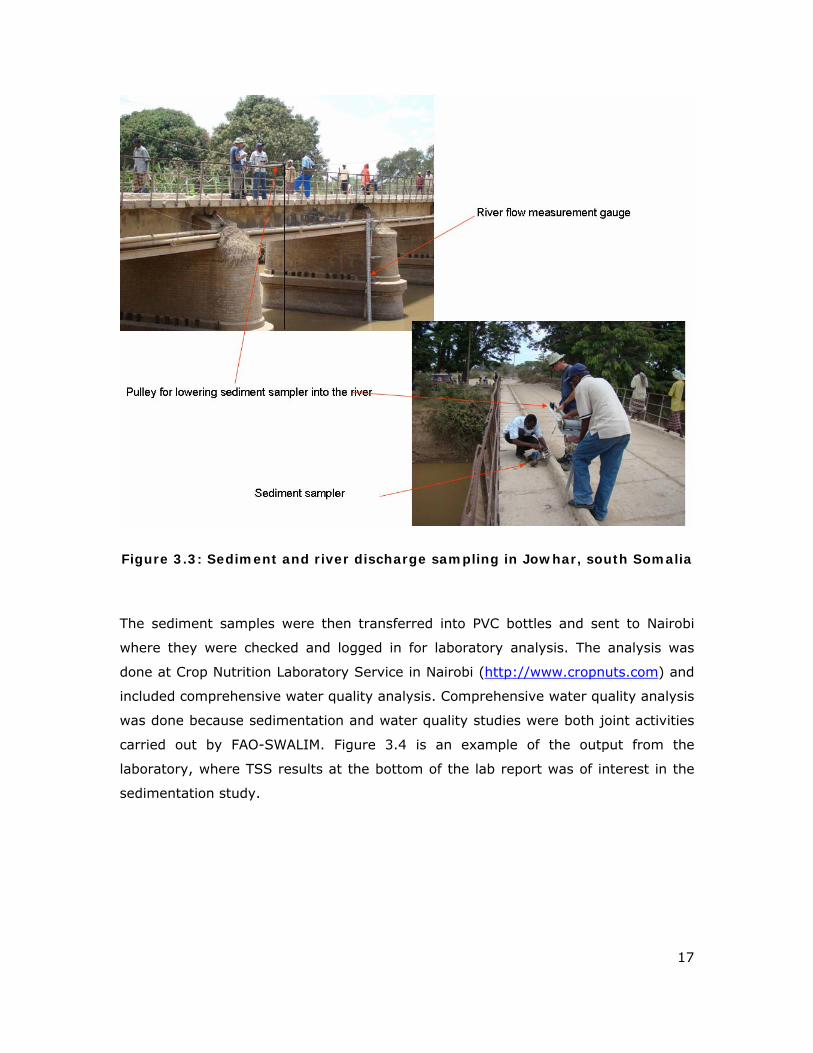
Figure 3.3: Sediment and river discharge sampling in Jowhar, south Somalia
The sediment samples were then transferred into PVC bottles and sent to Nairobi
where they were checked and logged in for laboratory analysis. The analysis was
done at Crop Nutrition Laboratory Service in Nairobi (http://www.cropnuts.com) and
included comprehensive water quality analysis. Comprehensive water quality analysis
was done because sedimentation and water quality studies were both joint activities
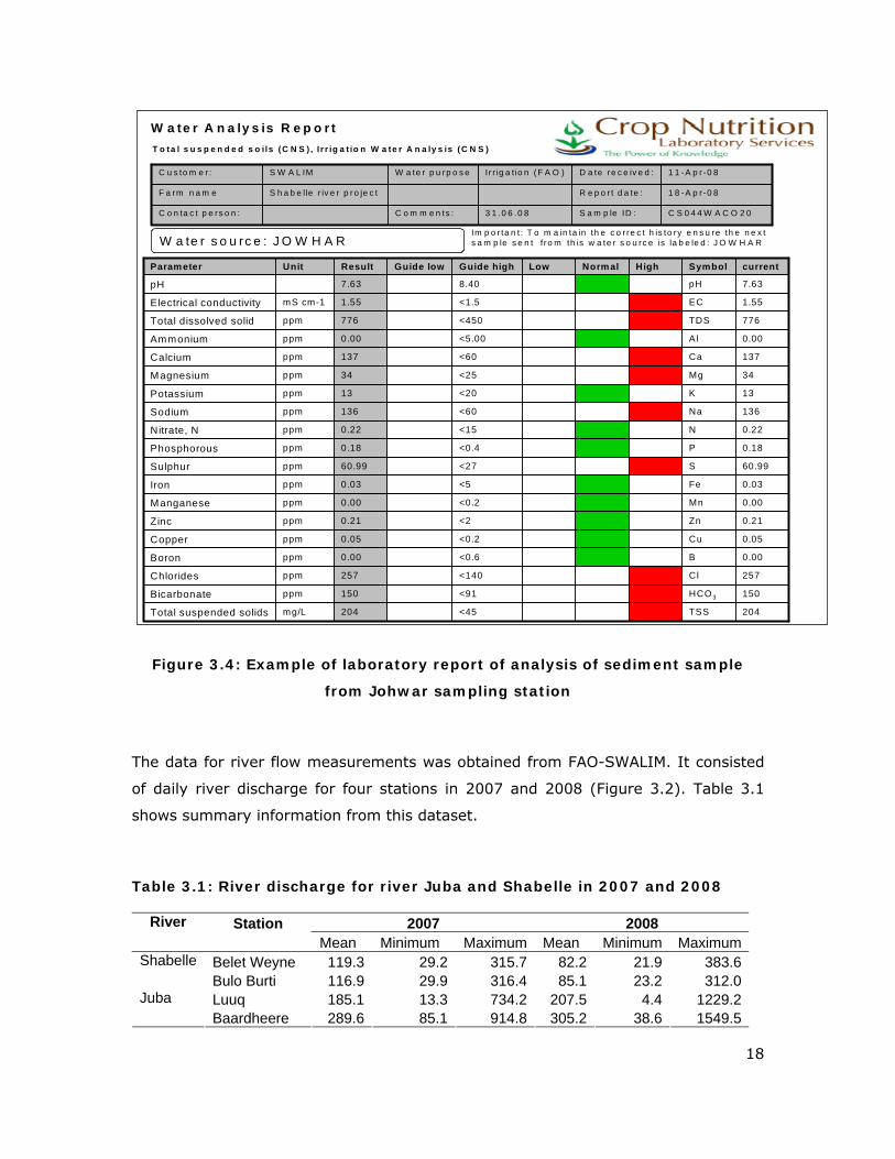
carried out by FAO-SWALIM. Figure 3.4 is an example of the output from the
laboratory, where TSS results at the bottom of the lab report was of interest in the
sedimentation study.
18
7.63pH8.407.63pH
204TSS<45204mg/LTotal suspended solids
150HCO3<91150ppmBicarbonate
257Cl<140257ppmChlorides
0.00B<0.60.00ppmBoron
0.05Cu<0.20.05ppmCopper
0.21Zn<20.21ppmZinc
0.00Mn<0.20.00ppmManganese
0.03Fe<50.03ppmIron
60.99S<2760.99ppmSulphur
0.18P<0.40.18ppmPhosphorous
0.22N<150.22ppmNitrate, N
136Na<60136ppmSodium
13K<2013ppmPotassium
34Mg<2534ppmMagnesium
137Ca<60137ppmCalcium
0.00Al<5.000.00ppmAmmonium
776TDS<450776ppmTotal dissolved solid
1.55EC<1.51.55mS cm-1Electrical conductivity
currentSymbolHighNormalLowGuide highGuide lowResultUnitParameter
W a te r A n a ly s is R e p o r tT o ta l s u s p e n d e d s o i ls (C N S ) , I r r ig a t io n W a te r A n a ly s is (C N S )
C S 0 4 4 W A C O 2 0S a m p le ID :3 1 .0 6 .0 8C o m m e n ts :C o n ta c t p e rs o n :
1 8 -A p r -0 8R e p o r t d a te :S h a b e lle r iv e r p ro je c tF a rm n a m e
1 1 -A p r -0 8D a te re c e iv e d :I r r ig a t io n (F A O )W a te r p u rp o s eS W A L IMC u s to m e r :
W a te r s o u rc e : J O W H A RIm p o r ta n t : T o m a in ta in th e c o r re c t h is to ry e n s u re th e n e x t s a m p le s e n t f ro m th is w a te r s o u rc e is la b e le d : J O W H A R
Figure 3.4: Example of laboratory report of analysis of sediment sample
from Johwar sampling station
The data for river flow measurements was obtained from FAO-SWALIM. It consisted
of daily river discharge for four stations in 2007 and 2008 (Figure 3.2). Table 3.1
shows summary information from this dataset.
Table 3.1: River discharge for river Juba and Shabelle in 2007 and 2008
River Station 2007 2008 Mean Minimum Maximum Mean Minimum Maximum
Belet Weyne 119.3 29.2 315.7 82.2 21.9 383.6Shabelle Bulo Burti 116.9 29.9 316.4 85.1 23.2 312.0Luuq 185.1 13.3 734.2 207.5 4.4 1229.2Juba Baardheere 289.6 85.1 914.8 305.2 38.6 1549.5
19
The summary shows that the flow rate in river Juba was higher than the flow rate in
river Shabelle in 2007 and 2008. Also, on average river Juba had higher flow in 2008
than in 2007 while river Shabelle had higher flow rate in 2007 than in 2008 (Table
3.1).
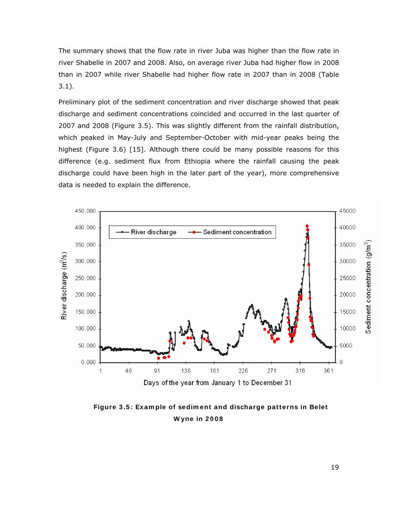
Preliminary plot of the sediment concentration and river discharge showed that peak
discharge and sediment concentrations coincided and occurred in the last quarter of
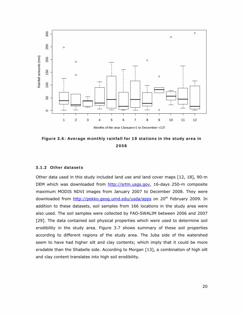
2007 and 2008 (Figure 3.5). This was slightly different from the rainfall distribution,
which peaked in May-July and September-October with mid-year peaks being the
highest (Figure 3.6) [15]. Although there could be many possible reasons for this
difference (e.g. sediment flux from Ethiopia where the rainfall causing the peak
discharge could have been high in the later part of the year), more comprehensive
data is needed to explain the difference.
Figure 3.5: Example of sediment and discharge patterns in Belet
Wyne in 2008
20
1 2 3 4 5 6 7 8 9 10 11 12
050
100
150
200
250
300
Months of the year (January=1 to December =12)
Rai
nfal
l am
ount
s (m
m)
Figure 3.6: Average monthly rainfall for 19 stations in the study area in
2008
3.1.2 Other datasets
Other data used in this study included land use and land cover maps [12, 18], 90-m
DEM which was downloaded from http://srtm.usgs.gov, 16-days 250-m composite
maximum MODIS NDVI images from January 2007 to December 2008. They were
downloaded from http://pekko.geog.umd.edu/usda/apps on 20th February 2009. In
addition to these datasets, soil samples from 166 locations in the study area were
also used. The soil samples were collected by FAO-SWALIM between 2006 and 2007
[29]. The data contained soil physical properties which were used to determine soil
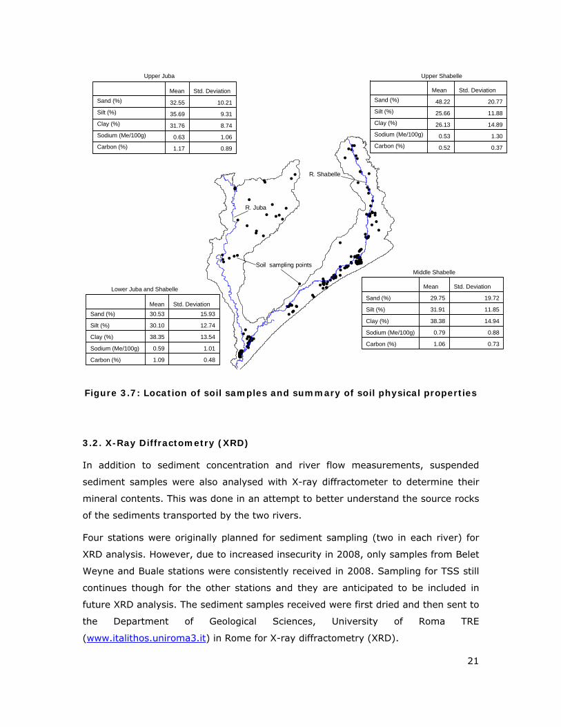
erodibility in the study area. Figure 3.7 shows summary of these soil properties
according to different regions of the study area. The Juba side of the watershed
seem to have had higher silt and clay contents; which imply that it could be more
erodable than the Shabelle side. According to Morgan [13], a combination of high silt
and clay content translates into high soil erodibility.
21
0.891.17Carbon (%)1.060.63Sodium (Me/100g)8.7431.76Clay (%)9.3135.69Silt (%)
10.2132.55Sand (%)Std. DeviationMean
0.370.52Carbon (%)1.300.53Sodium (Me/100g)
14.8926.13Clay (%)11.8825.66Silt (%)20.7748.22Sand (%)
Std. DeviationMean
0.731.06Carbon (%)
0.880.79Sodium (Me/100g)
14.9438.38Clay (%)
11.8531.91Silt (%)
19.7229.75Sand (%)
Std. DeviationMean
0.481.09Carbon (%)
1.010.59Sodium (Me/100g)
13.5438.35Clay (%)
12.7430.10Silt (%)
15.9330.53Sand (%)Std. DeviationMean
Lower Juba and Shabelle
Middle Shabelle
Upper ShabelleUpper Juba
########################
#
#######
##
#
###
######
####
#
####
###
###
#
#
##
#####
###
#
##
#
##
#
#
#########
#
#
#
####
#
#
# ##
#
#
###
##
####
##
### ##
#######################
##
##
##
## ##
#
###
###
###
#
#
#
#
#
#
#
##
#
#
###
##
##
#
#
###
# #
##
#
###
###
#
###
##
##
#
#
R. Juba
R. Shabelle
Soil sampling points
Figure 3.7: Location of soil samples and summary of soil physical properties
3.2. X-Ray Diffractometry (XRD)
In addition to sediment concentration and river flow measurements, suspended
sediment samples were also analysed with X-ray diffractometer to determine their
mineral contents. This was done in an attempt to better understand the source rocks
of the sediments transported by the two rivers.
Four stations were originally planned for sediment sampling (two in each river) for
XRD analysis. However, due to increased insecurity in 2008, only samples from Belet
Weyne and Buale stations were consistently received in 2008. Sampling for TSS still
continues though for the other stations and they are anticipated to be included in
future XRD analysis. The sediment samples received were first dried and then sent to
the Department of Geological Sciences, University of Roma TRE
(www.italithos.uniroma3.it) in Rome for X-ray diffractometry (XRD).
22
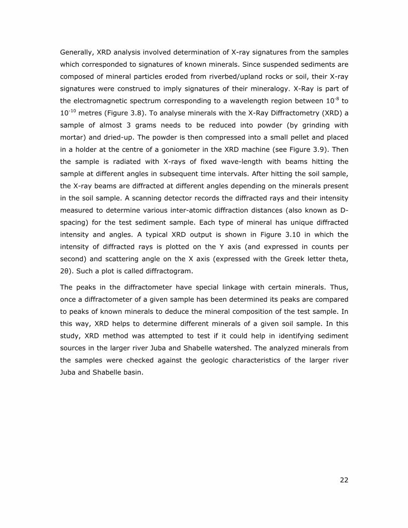
Generally, XRD analysis involved determination of X-ray signatures from the samples
which corresponded to signatures of known minerals. Since suspended sediments are
composed of mineral particles eroded from riverbed/upland rocks or soil, their X-ray
signatures were construed to imply signatures of their mineralogy. X-Ray is part of
the electromagnetic spectrum corresponding to a wavelength region between 10-8 to
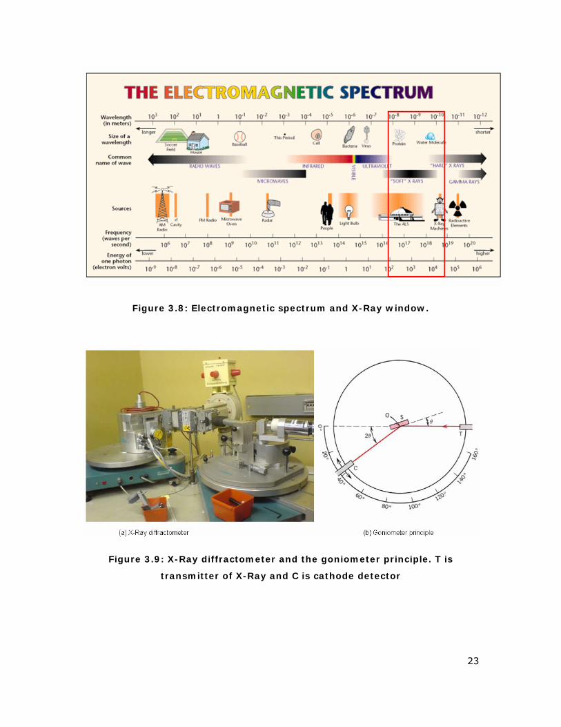
10-10 metres (Figure 3.8). To analyse minerals with the X-Ray Diffractometry (XRD) a
sample of almost 3 grams needs to be reduced into powder (by grinding with
mortar) and dried-up. The powder is then compressed into a small pellet and placed
in a holder at the centre of a goniometer in the XRD machine (see Figure 3.9). Then
the sample is radiated with X-rays of fixed wave-length with beams hitting the
sample at different angles in subsequent time intervals. After hitting the soil sample,
the X-ray beams are diffracted at different angles depending on the minerals present
in the soil sample. A scanning detector records the diffracted rays and their intensity
measured to determine various inter-atomic diffraction distances (also known as D-
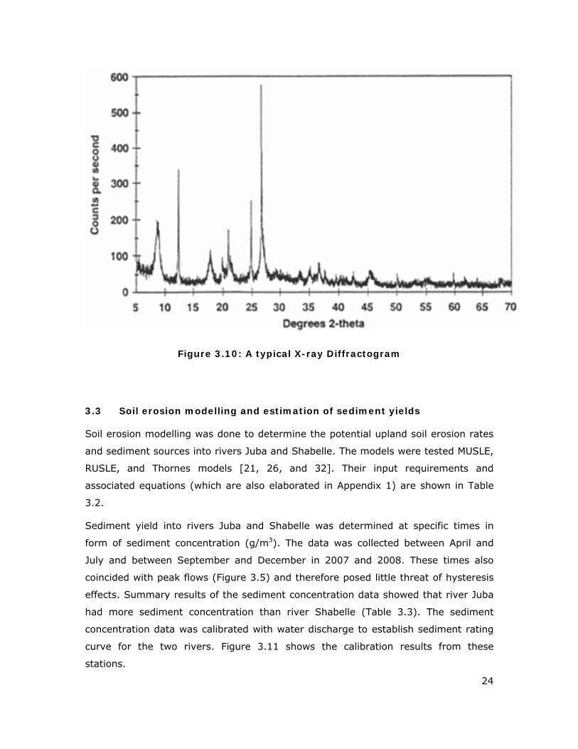
spacing) for the test sediment sample. Each type of mineral has unique diffracted
intensity and angles. A typical XRD output is shown in Figure 3.10 in which the
intensity of diffracted rays is plotted on the Y axis (and expressed in counts per
second) and scattering angle on the X axis (expressed with the Greek letter theta,
2θ). Such a plot is called diffractogram.
The peaks in the diffractometer have special linkage with certain minerals. Thus,
once a diffractometer of a given sample has been determined its peaks are compared
to peaks of known minerals to deduce the mineral composition of the test sample. In
this way, XRD helps to determine different minerals of a given soil sample. In this
study, XRD method was attempted to test if it could help in identifying sediment
sources in the larger river Juba and Shabelle watershed. The analyzed minerals from
the samples were checked against the geologic characteristics of the larger river
Juba and Shabelle basin.
23
Figure 3.8: Electromagnetic spectrum and X-Ray window.
Figure 3.9: X-Ray diffractometer and the goniometer principle. T is
transmitter of X-Ray and C is cathode detector
24
Figure 3.10: A typical X-ray Diffractogram
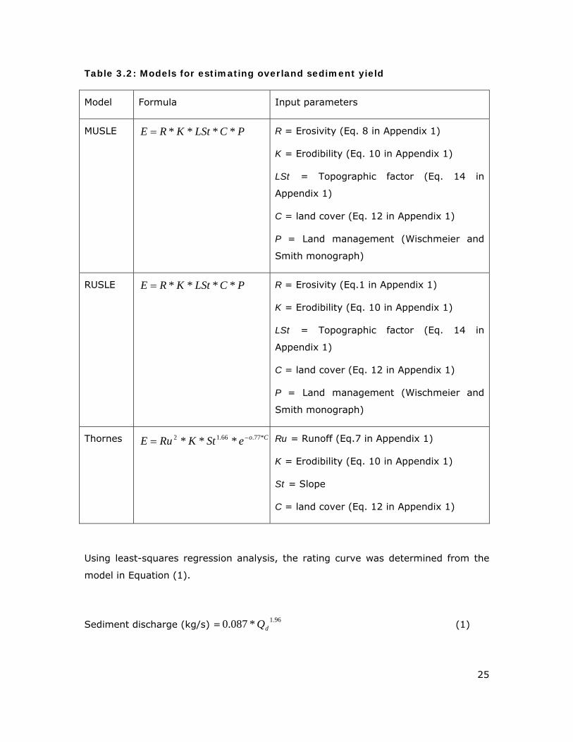
3.3 Soil erosion modelling and estimation of sediment yields
Soil erosion modelling was done to determine the potential upland soil erosion rates
and sediment sources into rivers Juba and Shabelle. The models were tested MUSLE,
RUSLE, and Thornes models [21, 26, and 32]. Their input requirements and
associated equations (which are also elaborated in Appendix 1) are shown in Table
3.2.
Sediment yield into rivers Juba and Shabelle was determined at specific times in
form of sediment concentration (g/m3). The data was collected between April and
July and between September and December in 2007 and 2008. These times also
coincided with peak flows (Figure 3.5) and therefore posed little threat of hysteresis
effects. Summary results of the sediment concentration data showed that river Juba
had more sediment concentration than river Shabelle (Table 3.3). The sediment
concentration data was calibrated with water discharge to establish sediment rating
curve for the two rivers. Figure 3.11 shows the calibration results from these
stations.
25
Table 3.2: Models for estimating overland sediment yield
Model Formula Input parameters
MUSLE
PCLStKRE ****= R = Erosivity (Eq. 8 in Appendix 1)
K = Erodibility (Eq. 10 in Appendix 1)
LSt = Topographic factor (Eq. 14 in
Appendix 1)
C = land cover (Eq. 12 in Appendix 1)
P = Land management (Wischmeier and
Smith monograph)
RUSLE
PCLStKRE ****= R = Erosivity (Eq.1 in Appendix 1)
K = Erodibility (Eq. 10 in Appendix 1)
LSt = Topographic factor (Eq. 14 in
Appendix 1)
C = land cover (Eq. 12 in Appendix 1)
P = Land management (Wischmeier and
Smith monograph)
Thornes
CoeStKRuE *77.66.12 *** −=
Ru = Runoff (Eq.7 in Appendix 1)
K = Erodibility (Eq. 10 in Appendix 1)
St = Slope
C = land cover (Eq. 12 in Appendix 1)
Using least-squares regression analysis, the rating curve was determined from the
model in Equation (1).
Sediment discharge (kg/s) =96.1*087.0 dQ (1)
26
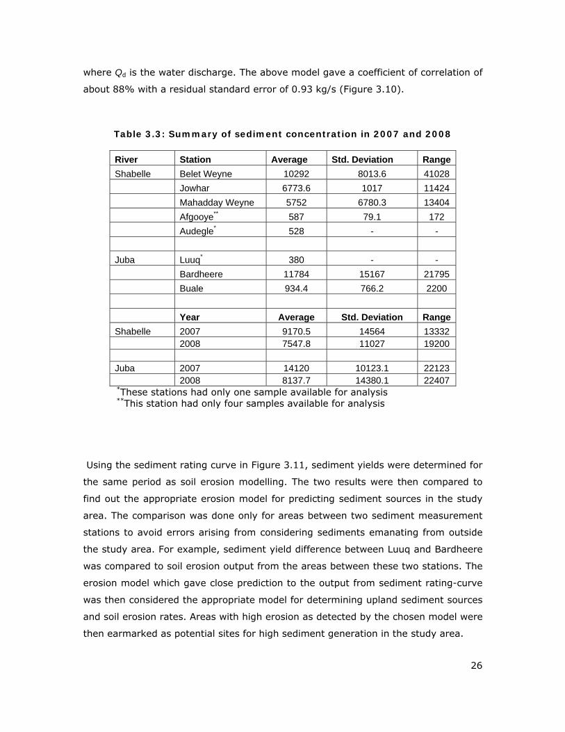
where Qd is the water discharge. The above model gave a coefficient of correlation of
about 88% with a residual standard error of 0.93 kg/s (Figure 3.10).
Table 3.3: Summary of sediment concentration in 2007 and 2008
River Station Average Std. Deviation Range Shabelle Belet Weyne 10292 8013.6 41028 Jowhar 6773.6 1017 11424 Mahadday Weyne 5752 6780.3 13404 Afgooye** 587 79.1 172 Audegle* 528 - - Juba Luuq* 380 - - Bardheere 11784 15167 21795 Buale 934.4 766.2 2200 Year Average Std. Deviation Range Shabelle 2007 9170.5 14564 13332 2008 7547.8 11027 19200 Juba 2007 14120 10123.1 22123 2008 8137.7 14380.1 22407
*These stations had only one sample available for analysis **This station had only four samples available for analysis
Using the sediment rating curve in Figure 3.11, sediment yields were determined for
the same period as soil erosion modelling. The two results were then compared to
find out the appropriate erosion model for predicting sediment sources in the study
area. The comparison was done only for areas between two sediment measurement
stations to avoid errors arising from considering sediments emanating from outside
the study area. For example, sediment yield difference between Luuq and Bardheere
was compared to soil erosion output from the areas between these two stations. The
erosion model which gave close prediction to the output from sediment rating-curve
was then considered the appropriate model for determining upland sediment sources
and soil erosion rates. Areas with high erosion as detected by the chosen model were
then earmarked as potential sites for high sediment generation in the study area.
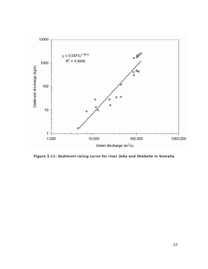
27
Figure 3.11: Sediment rating curve for river Juba and Shabelle in Somalia
28
4. RESULTS AND DISCUSSIONS
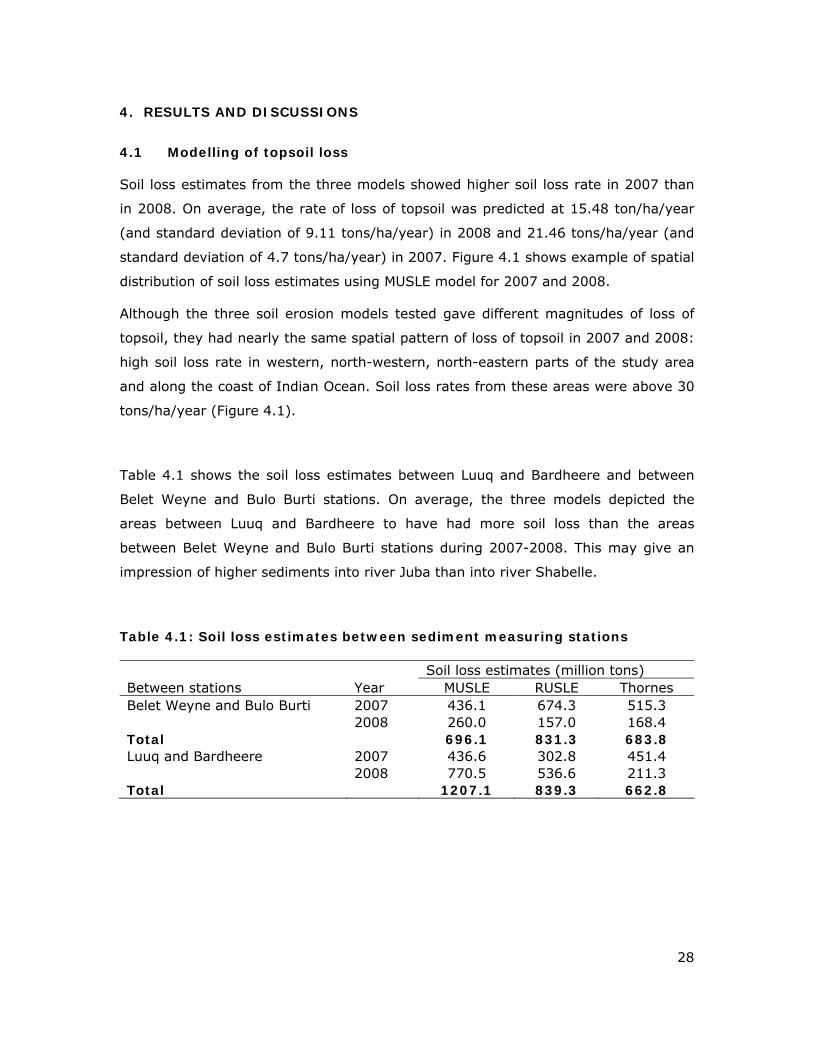
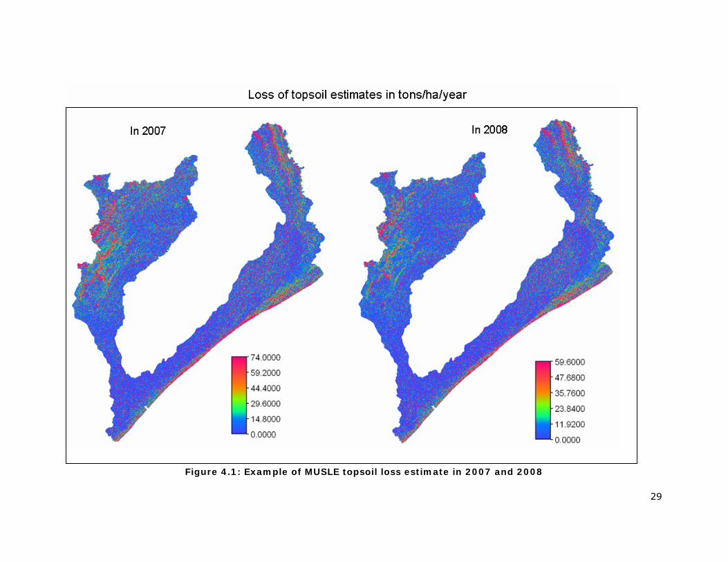
4.1 Modelling of topsoil loss
Soil loss estimates from the three models showed higher soil loss rate in 2007 than
in 2008. On average, the rate of loss of topsoil was predicted at 15.48 ton/ha/year
(and standard deviation of 9.11 tons/ha/year) in 2008 and 21.46 tons/ha/year (and
standard deviation of 4.7 tons/ha/year) in 2007. Figure 4.1 shows example of spatial
distribution of soil loss estimates using MUSLE model for 2007 and 2008.
Although the three soil erosion models tested gave different magnitudes of loss of
topsoil, they had nearly the same spatial pattern of loss of topsoil in 2007 and 2008:
high soil loss rate in western, north-western, north-eastern parts of the study area
and along the coast of Indian Ocean. Soil loss rates from these areas were above 30
tons/ha/year (Figure 4.1).
Table 4.1 shows the soil loss estimates between Luuq and Bardheere and between
Belet Weyne and Bulo Burti stations. On average, the three models depicted the
areas between Luuq and Bardheere to have had more soil loss than the areas
between Belet Weyne and Bulo Burti stations during 2007-2008. This may give an
impression of higher sediments into river Juba than into river Shabelle.
Table 4.1: Soil loss estimates between sediment measuring stations
Soil loss estimates (million tons) Between stations Year MUSLE RUSLE Thornes Belet Weyne and Bulo Burti 2007 436.1 674.3 515.3 2008 260.0 157.0 168.4 Total 696.1 831.3 683.8 Luuq and Bardheere 2007 436.6 302.8 451.4 2008 770.5 536.6 211.3 Total 1207.1 839.3 662.8
29
Figure 4.1: Example of MUSLE topsoil loss estimate in 2007 and 2008
30
4.2 Comparison of modelling and rating curve estimates of sediment yield
Sediment yield from the rating curve was determined every six months from January
2007 to December 2008. In order to try to account for sediment yield within the
study area alone, the sediment yield at upstream locations were subtracted from
sediment yield at the downstream stations (e.g. sediment yield at Bulo Burti minus
sediment yield at Belet Weyne). The outputs were then compared to topsoil loss
modelling estimates for the areas between these stations. Table 4.2 shows the
results of this comparison.
Table 4.2: Sediment yield from the rating curve compared with modelling
Estimation method (million tons) Between stations Period Rating curve MUSLE RUSLE Thornes
Belet Weyne - Bulo Burti 1st half 2007 580.0 256.1 471.2 402.5 2nd half 2007 211.2 180.0 203.1 112.9 1st half 2008 182.1 169.8 45.8 101.2 2nd half 2008 123.8 90.2 111.2 67.2 Luuq - Bardheere 1st half 2007 186.5 44.6 68.0 150.3 2nd half 2007 534.7 332.1 234.8 301.1 1st half 2008 951.7 785.5 523.8 118.1 2nd half 2008 123.7 45.0 12.8 93.2 Sum of Squared Error (SEE) 202166 431780 995277
The sediment yield by rating curve gave higher estimates between Luuq and
Bardheere than between Belet Weyne and Bulo Burti. The other three soil loss
models also gave similar estimate; thus, corroborating the impression depicted by
the rating curve that sediments into river Juba were higher than sediments into river
Shabelle. Before concluding that there could be higher sediments into river Juba than
Shabelle, a number of possible facts were considered: the area, river flow rate, and
topography of the areas between the gauging stations. In terms of areas, the area
between Belet Weyne and Bulo Burti was 22% of the area between Luuq and
Baardheere; which imply that sediment contributing areas in river Juba was larger
than in river Shabelle. In Table 3.1 it was shown that river Juba flow rate was higher
than river Shabelle; again indicating that river Juba had potentially more energy to
31
carry more sediment than river Shabelle. In terms of topography, the area between
Luuq and Baardheere is flanking to highly eroding plateau and had high content of
easily erodable soil material (Figure 3.7). The topography of the area between Belet
Weyne and Bulo Burti is mainly rocky ridges on the eastern side of the river with less
eroding soil material. These characteristics show that the sediment yield between
Luuq and Bardheere should be higher than between Belet Weyne and Bulo Burti. This
was in fact confirmed from the sediment yield results (Table 4.2) where the average
six-month sediment yield between Belet Weyne and Bulo Burti was 82% of the
sediment yield between Luuq and Bardheere.
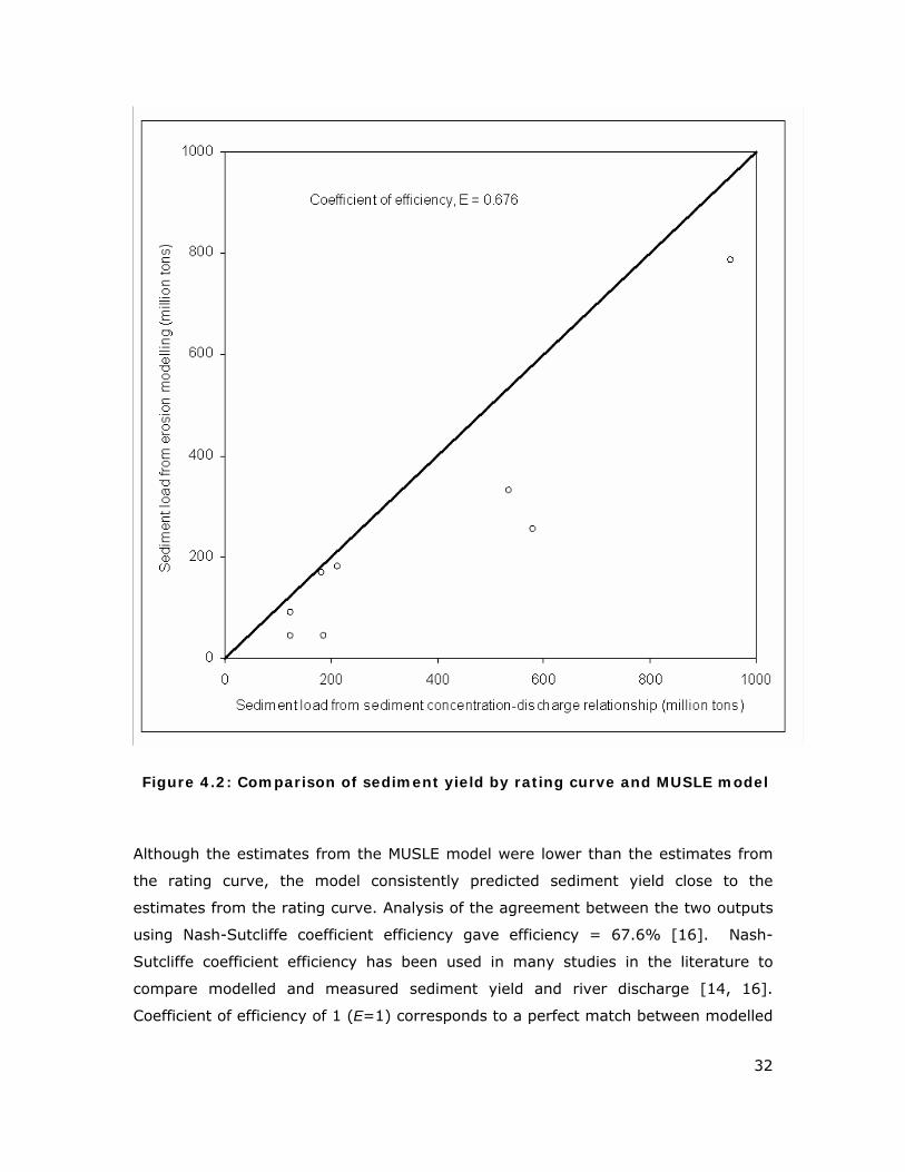
Comparison of the sediment yield from the rating curve and modelling estimates
showed that MUSLE model had the closest estimates to the rating curve outputs
(Table 4.2). Figure 4.2 shows the relationship between the estimates from the rating
curve and MUSLE outputs. The bold diagonal line in the figure is a 1:1 comparison
line (i.e. where the two estimates of sediment yields would ideally fall if they were
similar). As it is, sediment yield from the rating curve was higher than sediment yield
from erosion modelling. Perhaps this was because erosion modelling did not account
for channel erosion and bedload which were already included in the rating curve
outputs.
32
Figure 4.2: Comparison of sediment yield by rating curve and MUSLE model
Although the estimates from the MUSLE model were lower than the estimates from
the rating curve, the model consistently predicted sediment yield close to the
estimates from the rating curve. Analysis of the agreement between the two outputs
using Nash-Sutcliffe coefficient efficiency gave efficiency = 67.6% [16]. Nash-
Sutcliffe coefficient efficiency has been used in many studies in the literature to
compare modelled and measured sediment yield and river discharge [14, 16].
Coefficient of efficiency of 1 (E=1) corresponds to a perfect match between modelled
33
and observed data. Efficiency of 0 (E=0) indicates that the model predictions are as
accurate as the mean of the observed data, whereas an efficiency less than zero (-
∞<E<0) occurs when the observed mean is a better predictor than the model [14].
In the case of sediment yield in rivers Juba and Shabelle, the soil loss modelling by
MUSLE can be said to have had fairly close approximation to sediment yield
measurements in 2007 and 2008. Hence, MUSLE soil loss estimate could be regarded
as a good predictor of sediment yield in the study area.
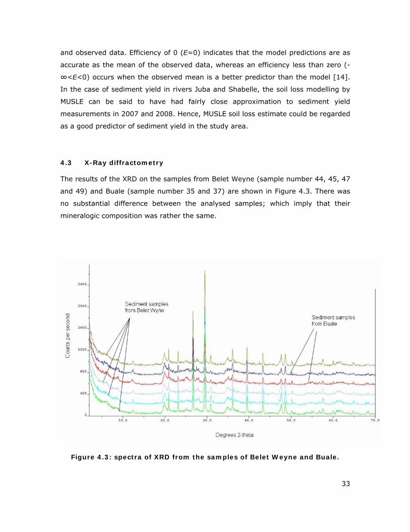
4.3 X-Ray diffractometry
The results of the XRD on the samples from Belet Weyne (sample number 44, 45, 47
and 49) and Buale (sample number 35 and 37) are shown in Figure 4.3. There was
no substantial difference between the analysed samples; which imply that their
mineralogic composition was rather the same.
Figure 4.3: spectra of XRD from the samples of Belet Weyne and Buale.
34
The XRD laboratory report also specified that there was no major difference between
the sediment samples analysed. The report also showed that all the sediment
samples analysed had residual minerals such as calcite, quartz, and feldspar and
neo-formation minerals such as chlorite, kaolinite, smectite, illite. See Appendix 2 for
definition of these minerals.
Te XRD results shown in Figure 4.3 were quite uniform since they come from one
sample for each river only (due to field inaccessibility). Having one sample at each
river means that the suspended sediment contains minerals from most of the rocks
outcropping upstream of the sampling point.
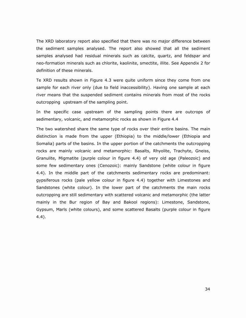
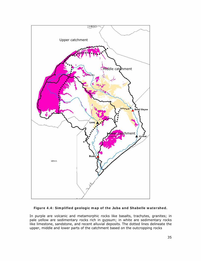
In the specific case upstream of the sampling points there are outcrops of
sedimentary, volcanic, and metamorphic rocks as shown in Figure 4.4
The two watershed share the same type of rocks over their entire basins. The main
distinction is made from the upper (Ethiopia) to the middle/lower (Ethiopia and
Somalia) parts of the basins. In the upper portion of the catchments the outcropping
rocks are mainly volcanic and metamorphic: Basalts, Rhyolite, Trachyte, Gneiss,
Granulite, Migmatite (purple colour in figure 4.4) of very old age (Paleozoic) and
some few sedimentary ones (Cenozoic): mainly Sandstone (white colour in figure
4.4). In the middle part of the catchments sedimentary rocks are predominant:
gypsiferous rocks (pale yellow colour in figure 4.4) together with Limestones and
Sandstones (white colour). In the lower part of the catchments the main rocks
outcropping are still sedimentary with scattered volcanic and metamorphic (the latter
mainly in the Bur region of Bay and Bakool regions): Limestone, Sandstone,
Gypsum, Marls (white colours), and some scattered Basalts (purple colour in figure
4.4).
35
Figure 4.4: Simplified geologic map of the Juba and Shabelle watershed.
In purple are volcanic and metamorphic rocks like basalts, trachytes, granites; in pale yellow are sedimentary rocks rich in gypsum; in white are sedimentary rocks like limestone, sandstone, and recent alluvial deposits. The dotted lines delineate the upper, middle and lower parts of the catchment based on the outcropping rocks
Upper catchment
Middle catchment
Lower catchment
36
analysed samples were few and were collected during low river flows. It was
therefore unlikely that they could show major differences with respect to potential
geologic composition of upland areas. However, the XRD results carry some potential
for scientifically objective method for determining sediments sources in a watershed.
It is anticipated that in future more samples will be taken and detailed XRD analysis
done for comprehensive identification of sediment sources in the study area.
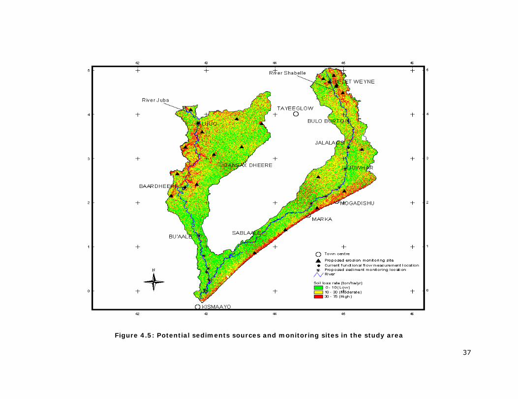
4.4 Potential sites for monitoring sediments
The potential sources of sediments into river Juba and Shabelle were identified from
the MUSLE modelling of upland topsoil loss. Figure 4.5 shows areas which were
consistently modelled by MUSLE as having high topsoil loss rates (> 30
tons/ha/year). They were therefore considered as potential sites contributing to high
sedimentation of rivers Juba and Shabelle.
Majority of the areas identified with high rate of topsoil loss (Figure 4.5) were also
found to belong to areas with low vegetation cover where transhumance
pastoralism/wood collection was the dominant type of land use [18]. It was therefore
possible to posit that overgrazing and deforestation were the major contributors to
high sediment yield from these areas. Along the coastline, sand dunes, pastoralism,
and negative effects of urbanization were the dominant land use types in areas with
high rates of topsoil loss. Again, the major contributors of high sediment yield from
these areas could have been transhumance pastoralism, urban centres, and
prevalent sand dunes.
If a quantitative analysis of land cover and land use change over time (at least the
last 10 years) would be available then more detailed considerations about the links
between land use/cover and soil erosion could be established.
37
Figure 4.5: Potential sediments sources and monitoring sites in the study area
38
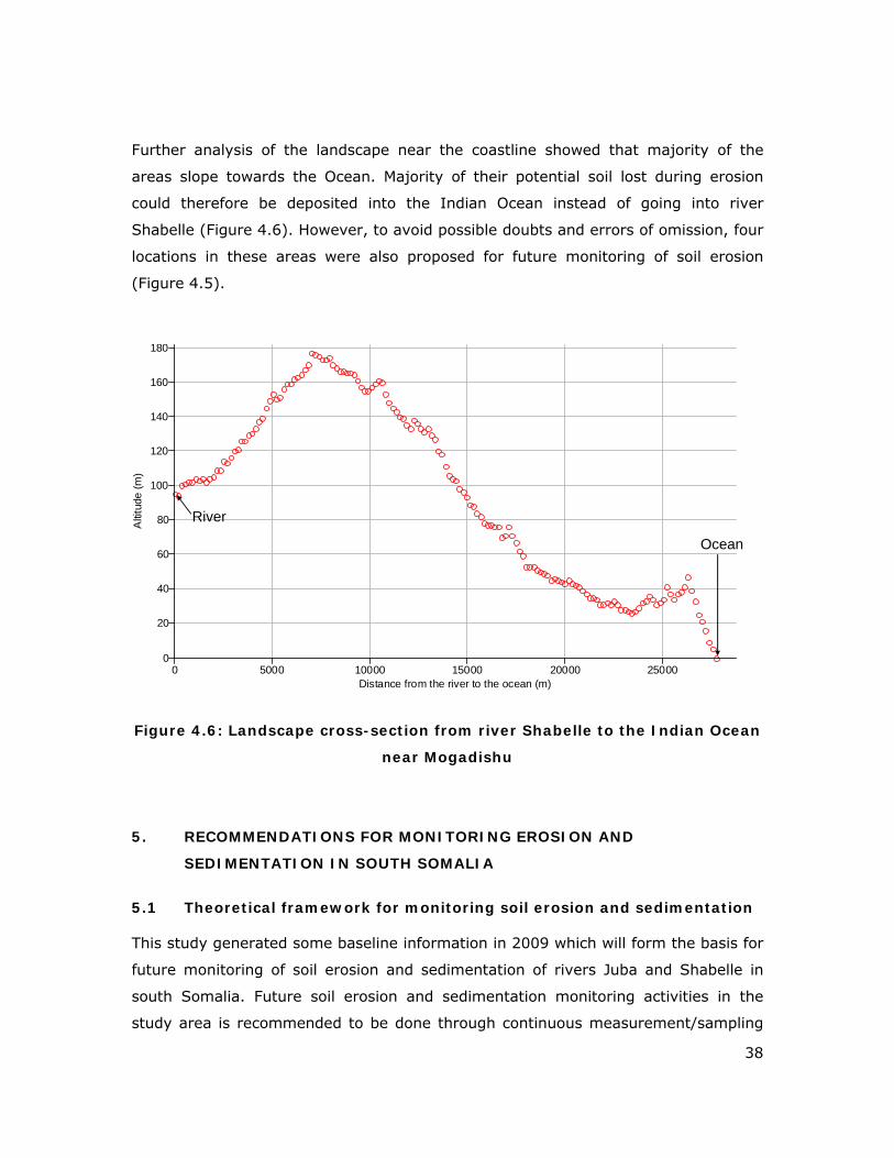
Further analysis of the landscape near the coastline showed that majority of the
areas slope towards the Ocean. Majority of their potential soil lost during erosion
could therefore be deposited into the Indian Ocean instead of going into river
Shabelle (Figure 4.6). However, to avoid possible doubts and errors of omission, four
locations in these areas were also proposed for future monitoring of soil erosion
(Figure 4.5).
0 5000 10000 15000 20000 25000Distance from the river to the ocean (m)
0
20
40
60
80
100
120
140
160
180
Alti
tude
(m)
River
Ocean
Figure 4.6: Landscape cross-section from river Shabelle to the Indian Ocean
near Mogadishu
5. RECOMMENDATIONS FOR MONITORING EROSION AND
SEDIMENTATION IN SOUTH SOMALIA
5.1 Theoretical framework for monitoring soil erosion and sedimentation
This study generated some baseline information in 2009 which will form the basis for
future monitoring of soil erosion and sedimentation of rivers Juba and Shabelle in
south Somalia. Future soil erosion and sedimentation monitoring activities in the
study area is recommended to be done through continuous measurement/sampling
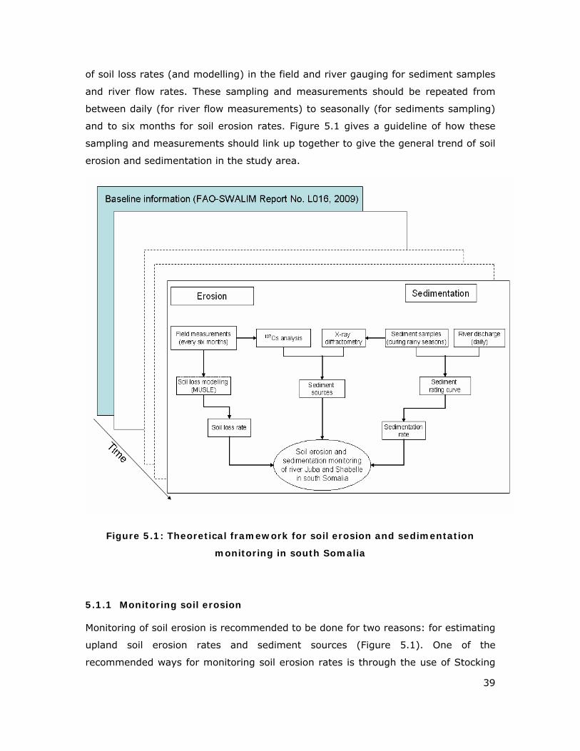
39
of soil loss rates (and modelling) in the field and river gauging for sediment samples
and river flow rates. These sampling and measurements should be repeated from
between daily (for river flow measurements) to seasonally (for sediments sampling)
and to six months for soil erosion rates. Figure 5.1 gives a guideline of how these
sampling and measurements should link up together to give the general trend of soil
erosion and sedimentation in the study area.
Figure 5.1: Theoretical framework for soil erosion and sedimentation
monitoring in south Somalia
5.1.1 Monitoring soil erosion
Monitoring of soil erosion is recommended to be done for two reasons: for estimating
upland soil erosion rates and sediment sources (Figure 5.1). One of the
recommended ways for monitoring soil erosion rates is through the use of Stocking
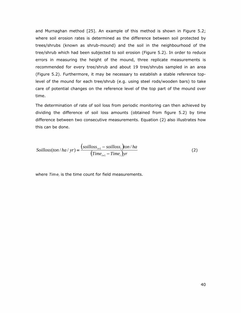
40
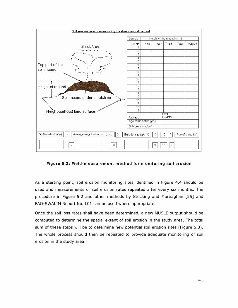
and Murnaghan method [25]. An example of this method is shown in Figure 5.2;
where soil erosion rates is determined as the difference between soil protected by
trees/shrubs (known as shrub-mound) and the soil in the neighbourhood of the
tree/shrub which had been subjected to soil erosion (Figure 5.2). In order to reduce
errors in measuring the height of the mound, three replicate measurements is
recommended for every tree/shrub and about 19 tree/shrubs sampled in an area
(Figure 5.2). Furthermore, it may be necessary to establish a stable reference top-
level of the mound for each tree/shrub (e.g. using steel rods/wooden bars) to take
care of potential changes on the reference level of the top part of the mound over
time.
The determination of rate of soil loss from periodic monitoring can then achieved by
dividing the difference of soil loss amounts (obtained from figure 5.2) by time
difference between two consecutive measurements. Equation (2) also illustrates how
this can be done.
( )( )yrTimeTime
hatonsoillosssoillossyrhatonSoilloss
ii
ii
−−
=+
+
1
1 /)//( (2)
where Timei is the time count for field measurements.
41
Figure 5.2: Field-measurement method for monitoring soil erosion
As a starting point, soil erosion monitoring sites identified in Figure 4.4 should be
used and measurements of soil erosion rates repeated after every six months. The
procedure in Figure 5.2 and other methods by Stocking and Murnaghan [25] and
FAO-SWALIM Report No. L01 can be used where appropriate.
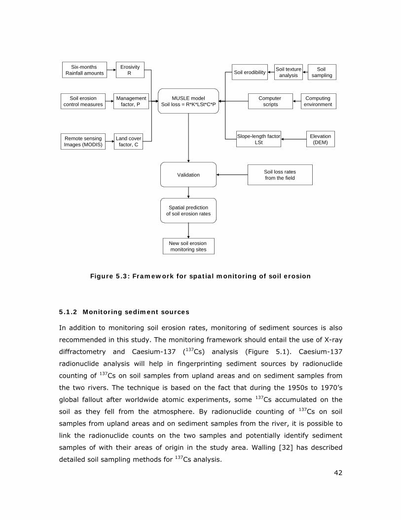
Once the soil loss rates shall have been determined, a new MUSLE output should be
computed to determine the spatial extent of soil erosion in the study area. The total
sum of these steps will be to determine new potential soil erosion sites (Figure 5.3).
The whole process should then be repeated to provide adequate monitoring of soil
erosion in the study area.
42
Soil loss ratesfrom the field
MUSLE modelSoil loss = R*K*LSt*C*P
ErosivityR
Six-months Rainfall amounts
Soil textureanalysisSoil erodibility Soil
sampling
Land coverfactor, C
Remote sensingImages (MODIS)
Managementfactor, P
Soil erosioncontrol measures
Elevation(DEM)
Slope-length factorLSt
Spatial predictionof soil erosion rates
New soil erosion monitoring sites
Computing environment
Computer scripts
Validation
Figure 5.3: Framework for spatial monitoring of soil erosion
5.1.2 Monitoring sediment sources
In addition to monitoring soil erosion rates, monitoring of sediment sources is also
recommended in this study. The monitoring framework should entail the use of X-ray
diffractometry and Caesium-137 (137Cs) analysis (Figure 5.1). Caesium-137
radionuclide analysis will help in fingerprinting sediment sources by radionuclide
counting of 137Cs on soil samples from upland areas and on sediment samples from
the two rivers. The technique is based on the fact that during the 1950s to 1970’s
global fallout after worldwide atomic experiments, some 137Cs accumulated on the
soil as they fell from the atmosphere. By radionuclide counting of 137Cs on soil
samples from upland areas and on sediment samples from the river, it is possible to
link the radionuclide counts on the two samples and potentially identify sediment
samples of with their areas of origin in the study area. Walling [32] has described
detailed soil sampling methods for 137Cs analysis.
43
Similarly, XRD may also be done on sediment samples to augment the results from 137Cs analysis. XRD analysis can detect sediment samples from a wider region
compared to 137Cs since it relates the minerals in the sediments samples to rock
materials in the wider river basin. Co-analysis of sediment samples by XRD and 137Cs
is recommended since the same sediment samples can be used for both methods;
hence there will be no need for separate sampling for XRD tests. In addition,
collaboration between FAO-SWALIM and institutions in Europe with specialized
laboratories for XRD and 137Cs is currently underway and is anticipated to benefit
sediment analysis by these two methods.
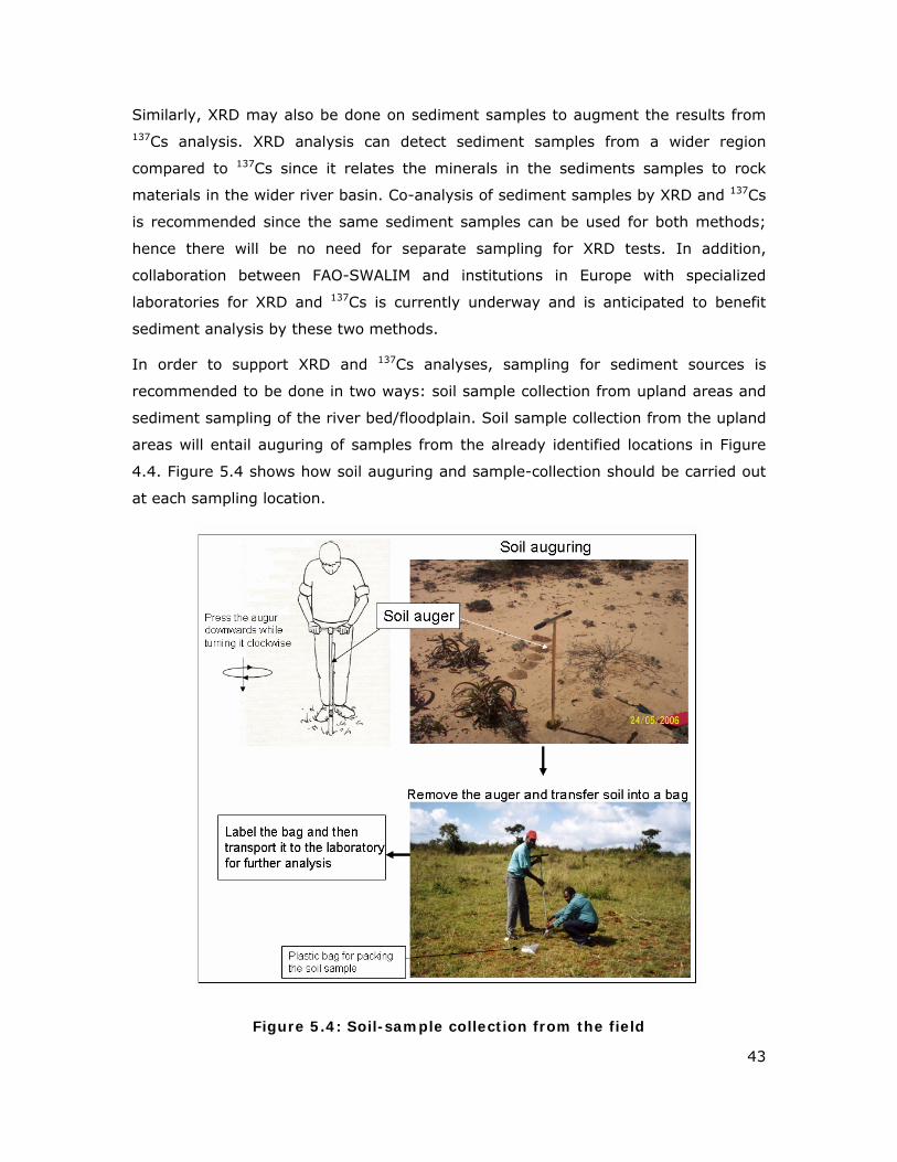
In order to support XRD and 137Cs analyses, sampling for sediment sources is
recommended to be done in two ways: soil sample collection from upland areas and
sediment sampling of the river bed/floodplain. Soil sample collection from the upland
areas will entail auguring of samples from the already identified locations in Figure
4.4. Figure 5.4 shows how soil auguring and sample-collection should be carried out
at each sampling location.
Figure 5.4: Soil-sample collection from the field
44
Sediment sampling of the river bed/floodplain will involve coring of floodplain and/or
river bed up to almost 1 m of depth and collecting samples of at least 50 g every 1
or 2 cm (depending on the rate of accretion). Soil augurs such as shown in Figure
5.4 can also be used for sediment coring. An estimate of the bulk density of the
sediment should also be done in the field in order to calculate the soil volume needed
to reach 50 g sample. Once the samples are collected, they will be transported to
specialized laboratories for XRD and 137Cs analysis.
5.1.3 Monitoring suspended sediment discharge
Due to cost of analysis for sampling and processing suspended sediment samples,
targeted sampling is recommended. The proposed locations chosen for suspended
sediment sampling in Figure 4.4 were those which coincided with locations for river
flow measurements. However, some of the river flow measurement locations have
been non-operational (see Figure 5.5) but are currently under consideration for
rehabilitation by FAO-SWALIM. It is recommended that the sediment samples from
these stations be taken and analysed alongside samples from the other operational
stations once the rehabilitation of non-operational gauging stations shall have been
completed. This will improve the sediment rating curve developed during this study.
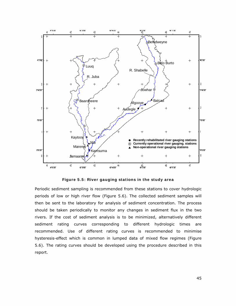
45
$
$
$
$
$
$
#Y
#Y
#Y
#Y
#Y
#Y
#
#
Afgooye
Audegle
Luuq
Baardheere
Jowhar
Bulo Burto
Beledweyne
KaytooyJilib
MarereyKamsuma
Jamaame
Balcad
R. Juba
R. Shabelle
$ Non-operational river gauging stations#Y Currently operational river gauging. stations# Recently rehabilitated river gauging stations
0°15'30" 0°15'30"
1°31'00" 1°31'00"
2°46'30" 2°46'30"
4°2'00" 4°2'00"
41°15'30"
41°15'30"
42°31'00"
42°31'00"
43°46'30"
43°46'30"
45°2'00"
45°2'00"
46°17'30"
46°17'30"41
41
42
42
43
43
44
44
45
45
46
46
47
47
0 0
1 1
2 2
3 3
4 4
5 5
Figure 5.5: River gauging stations in the study area
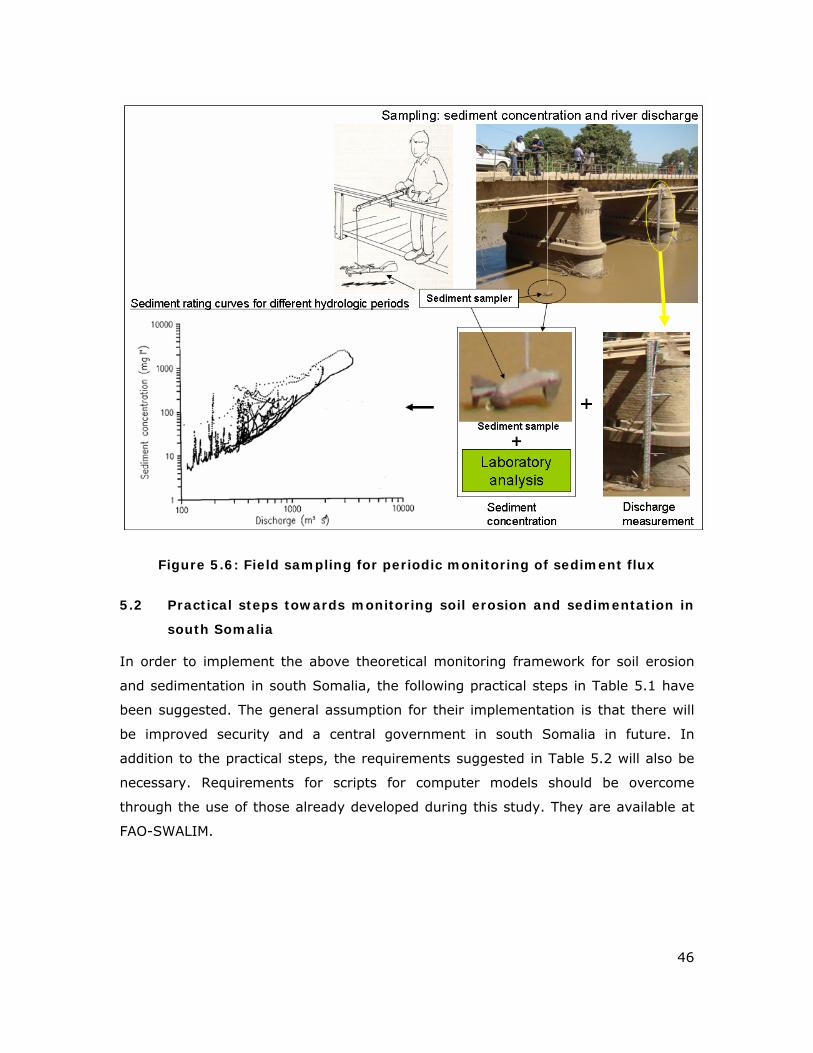
Periodic sediment sampling is recommended from these stations to cover hydrologic
periods of low or high river flow (Figure 5.6). The collected sediment samples will
then be sent to the laboratory for analysis of sediment concentration. The process
should be taken periodically to monitor any changes in sediment flux in the two
rivers. If the cost of sediment analysis is to be minimized, alternatively different
sediment rating curves corresponding to different hydrologic times are
recommended. Use of different rating curves is recommended to minimise
hysteresis-effect which is common in lumped data of mixed flow regimes (Figure
5.6). The rating curves should be developed using the procedure described in this
report.
46
Figure 5.6: Field sampling for periodic monitoring of sediment flux
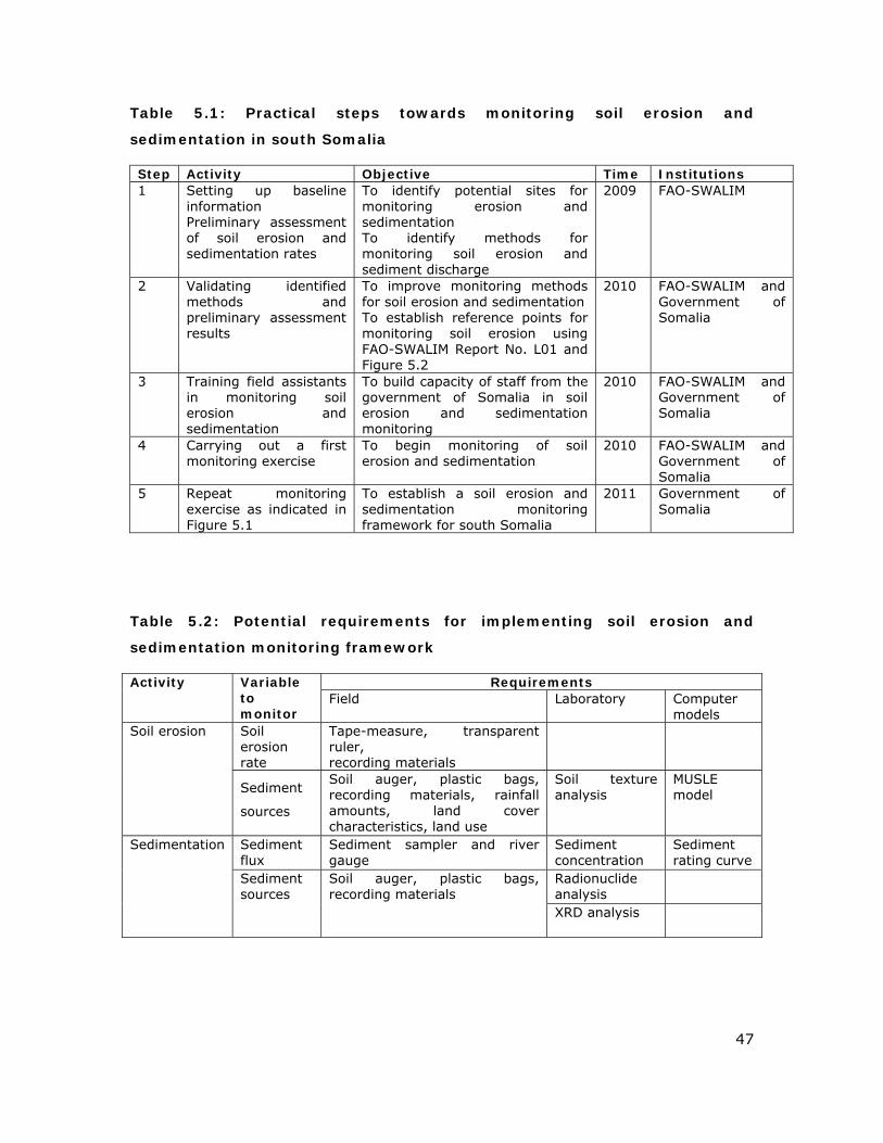
5.2 Practical steps towards monitoring soil erosion and sedimentation in
south Somalia
In order to implement the above theoretical monitoring framework for soil erosion
and sedimentation in south Somalia, the following practical steps in Table 5.1 have
been suggested. The general assumption for their implementation is that there will
be improved security and a central government in south Somalia in future. In
addition to the practical steps, the requirements suggested in Table 5.2 will also be
necessary. Requirements for scripts for computer models should be overcome
through the use of those already developed during this study. They are available at
FAO-SWALIM.
47
Table 5.1: Practical steps towards monitoring soil erosion and
sedimentation in south Somalia
Step Activity Objective Time Institutions 1 Setting up baseline
information Preliminary assessment of soil erosion and sedimentation rates
To identify potential sites for monitoring erosion and sedimentation To identify methods for monitoring soil erosion and sediment discharge
2009 FAO-SWALIM
2 Validating identified methods and preliminary assessment results
To improve monitoring methods for soil erosion and sedimentation To establish reference points for monitoring soil erosion using FAO-SWALIM Report No. L01 and Figure 5.2
2010 FAO-SWALIM and Government of Somalia
3 Training field assistants in monitoring soil erosion and sedimentation
To build capacity of staff from the government of Somalia in soil erosion and sedimentation monitoring
2010 FAO-SWALIM and Government of Somalia
4 Carrying out a first monitoring exercise
To begin monitoring of soil erosion and sedimentation
2010 FAO-SWALIM and Government of Somalia
5 Repeat monitoring exercise as indicated in Figure 5.1
To establish a soil erosion and sedimentation monitoring framework for south Somalia
2011 Government of Somalia
Table 5.2: Potential requirements for implementing soil erosion and
sedimentation monitoring framework
Requirements Activity Variable to monitor
Field Laboratory Computer models
Soil erosion rate
Tape-measure, transparent ruler, recording materials
Soil erosion
Sediment
sources
Soil auger, plastic bags, recording materials, rainfall amounts, land cover characteristics, land use
Soil texture analysis
MUSLE model
Sediment flux
Sediment sampler and river gauge
Sediment concentration
Sediment rating curve
Radionuclide analysis
Sedimentation
Sediment sources
Soil auger, plastic bags, recording materials
XRD analysis
48
6. CONCLUSIONS AND RECOMMENDATIONS
6.1 Conclusions
6.1.1 Potential sources of sediments
This study showed that river Juba which has higher discharge than Shabelle is
potentially carrying more sediments than river Shabelle. The sediment load into river
Juba in 2007 and 2008 was found to be about four times the sediment load in river
Shabelle in the same period. Some of this sediment load was found to originate from
the upland areas of the riverine areas of river Juba and Shabelle in south Somalia.
Analysis of potential soil erosion rates in the upland areas showed that annual loss of
topsoil in 2007 and 2008 was about 18 ton/ha. The major land use types driving this
rate of topsoil loss are livestock grazing, fuelwoood collection, and negative effects of
expansion of urban centres. These land use characteristics should be further
investigated and targeted for proper management to reduce the high soil erosion
rates in the study area.
6.1.2 Techniques and opportunities for monitoring sediments yields
Field measurement, modelling of soil erosion, and targeted sediment sampling of
river Juba and Shabelle were found in this study to be able to provide reliable
estimation of soil erosion and sedimentation rates. Their continuous measurement is
one way for monitoring soil erosion and sedimentation of the two rivers in south
Somalia. In addition to modelling and measurements, XRD and 137Cs radio-isotope
analysis are also potential indicators for identifying upland sediment sources. Their
analyses are potentially possible especially with the collaboration and support FAO-
SWALIM can get from the specialized laboratories in Europe who normally do such
analyses.
6.2 Recommendations
The following recommendations have been proposed as a way-forward for
implementing successful monitoring of soil erosion and sedimentation of river Juba
and Shabelle:
49
1. To carry out field validation of erosion modelling baseline generated during
this study. This should be done as soon as the security situation improves in
south Somalia.
2. To establish soil erosion monitoring reference sites and develop geodetic
survey protocol for insuring accuracy in measuring soil erosion rates.
3. Strengthening of the agreement and collaboration between FAO-SWALIM and
the government of Somalia and Ethiopia to support soil erosion and sediment
sampling of the greater river Juba and Shabelle watershed.
4. Rehabilitation of non-operational river gauging stations and incorporation of
sediment sampling alongside river flow measurements.
5. Establishment of routine and structured sample recording and processing
steps for sediment and soil samples for future laboratory analysis. A login
form is important for samples from the field to detail sample characteristics
(e.g. sampling date, georeference, etc).
6. Capacity building for the staff members of the relevant government ministries
in Somalia and Ethiopia with respect to soil erosion and sedimentation
monitoring of river Juba and Shabelle.
7. Follow up on 137Cs isotope and XRD analysis of more samples from the study
area and strengthening of collaboration between FAO-SWALIM, Somalia
government and institutions in Europe who are specialized in 137Cs and XRD
analysis of sediment samples.
8. More future support for continuation and implementation of soil erosion and
sedimentation monitoring within river Juba and Shabelle in Somalia and
Ethiopia.
9. Implementation of the proposed monitoring framework proposed in this
study.
Although all the above mentioned steps will be needed to put in place a thorough
scientific monitoring of soil erosion and sedimentation, some urgent measures to
prevent or reduce soil erosion should be adopted as soon as possible. This will
50
prevent further loss of fertile topsoil and increase soil productivity especially in
agricultural areas of the lower part of the river catchments.
Furthermore the not regulated tree cutting activity for charcoal production increases
the loss of top soil.
For this reason simple and cheap measure of soil conservation should be adopted
with immediate effect at least in the agricultural areas. For instance, on a short term,
properly designed soil bunds (soil and/or rock bunds) -in both the higher sloping
rainfed crop areas of Bay and Bakool regions and the low sloping irrigated areas
along the floodplains- should be created to allow accumulation of colluvium and
reduction of the erosive power of running waters. On a medium term, intervention
for mitigating the floods should be considered, in order to reduce the erosive power
of flooding waters over the prevalent clay soils of the study area. On a longer term,
and after adequate field assessment, the practice of agroforestry could be introduced
in the irrigated areas of the floodplains. In addition to this, in the few mechanized
farms of Lower and Middle Shabelle and along the Juba, contour stripping cropping
should be adopted to slow down the formation of straight runoff lines.
All the above mentioned counter measures, although probably not the most durable
in the long term, are efficient in the short terms, relatively cheap to put in practice
and culturally accepted and used in the Somali context as demonstrated by their
successful practice in other regions.
A proper flood control management and the rehabilitation of the canal system will
also allow for a better management of the moisture in the soil and of its drainage,
during both flood times and normal flows.
51
REFERENCES
1. Alim, A.S. 1997. Inventory report for Somalia. GCP/RAF/287/ITA Internal
Report No.1. FAO
2. Alonso, C.V., Bingner, R.L. and Kuhnle, R.A. 1995. Sediment yield from
watersheds with eroding channels. In: W.H. Espey and P.G. Combs (Editors),
Water Resources Engineering: Proceedings of the First International
Conference. American Society of Civil Engineers, pp. 1183-1187
3. Carbone, F. and Accordi, G. 2000. The Indian Ocean coast of Somalia.
Marine Pollution Bulletin 41:141-59. (Univ La Sapienza, CNR, Ctr Studio
Quaternario and Evoluz Ambientale, Dipartimento Sci Terra, P Aldo Moro, 5I-
00185 Rome, Italy
4. Collins, A.L. and Walling, D.E. 2002. Selecting fingerprint properties for
discriminating potential suspended sediment sources in river basins. J. of
Hydrology, 261(1-4): 218-244
5. Collins, A.L. and Walling, D.E. 2004. Documenting catchment suspended
sediment sources: problems, approaches and prospects. Progress in Physical
Geography, 28(2): 159-196
6. Collins, A.L., Walling, D.E., Sichingabula, H.M. and Leeks, G.J.L. 2001. Using
137 Cs measurements to quantify soil erosion and redistribution rates for
areas under different land use in the Upper Kaleya River Basin, Southern
Zambia. Geoderma, 104: 299-323.
7. Foster, G.R., 1982. Modelling the erosion processes. In: C.T. Haan (Editor),
Hydrologic Modelling of Small Watersheds. ASAE Monograph, pp. 297-380.
8. GTZ, 1990. Master plan for Juba Valley Development. Main Report. Somali
Democratic Republic
9. Hamin, R.S. and Doe, W.W. 2001. Landscape Erosion and Evolution
Modelling. Kluwer Academic / Plenum Publishers, New York, USA, 540 pp
10. Lu, X. and Higgitt, D.L. 2001. Sediment delivery to the Three Gorges. 2: local
response. Geomorphology, 41: 157-169.
11. McDonald and Partners in collaboration with Institute of Hydrology. 1991.
Hydrometry Project – Somalia. Final Report, Phase 3.
52
12. Monaci, L., Downie, M. And Oduori, S. 2007. Land Cover of Selected Study
Areas in Somaliland and Southern Somalia. FAO-SWALIM. Project Report No
L-03. , Nairobi, Kenya.
13. Morgan, R.P.C. 1986. Soil Erosion and Conservation. Longman Scientific &
Technical: Hong Kong
14. Moriasi, D. N. 2007. Model Evaluation Guidelines for Systematic Quantification
of Accuracy in Watershed Simulations. Transactions of the ASABE, 50(3):
885–900.
15. FAO-SWALIM Technical Report No W-01: Muchiri, P.W. 2007. Climate of
Somalia. Nairobi, Kenya.
16. Nash, J. E. and Sutcliffe, J. V. 1970. River flow forecasting through conceptual
models part I — A discussion of principles. Journal of Hydrology, 10 (3): 282–
290.
17. Nichols, M.H. and Renard, K.G. 1999. Sediment yield from semi-arid
watersheds, Agricultural Research Service, Southwest Watershed Research
Center, Tucson, USA
18. FAO-SWALIM Technical Report No L-07: Oduori, S.M., Vargas, R.R. and Alim,
M.S. 2007. Land use characterization of the Juba and Shabelle riverine areas
in Southern Somalia. Nairobi, Kenya
19. Omuto, C.T. and Vargas, R.R. 2009. Combining pedometrics, remote sensing
and field observations for assessing soil loss in challenging drylands: a case
study of North-western Somalia. Land Degradation and Development 20:
101-115.
20. Poesen, J., Nachtergaele, J., Verstraeten, G. and Valentin, C., 2003. Gully
erosion and environmental change: Importance and research needs. Catena,
50: 91-113
21. Renard, K.G., Foster, G.R., Weesies, G.A., McCool, D.K. and Yoder, D.C.
1997. Predicting Soil Erosion by Water: A Guide to Conservation Planning
With the Revised Universal Soil Loss Equation (RUSLE). USDA Agricultural
Handbook 703
53
22. Saavedra, C. 2005. Estimating spatial patterns of soil erosion and deposition
in the Andean region using geo-information techniques. A case study in
Cochabamba, Bolivia. PhD Thesis, ITC, Enschede
23. Soil Conservation Service (SCS), 1972. U.S.D.A., National Engineering
Handbook, Section 4: Hydrology. Washington DC.
24. Springer, G.S., Dowdy, H.S. and Eaton, L.S. 2001. Sediment budgets for two
mountainous basins affected by a catastrophic storm: Blue Ridge Mountains,
Virginia. Geomorphology, 37: 135-148
25. Stocking, M. and Murnaghan, N. 2001. Land degradation-Guidelines for field
assessment. University of East Anglia. Norwich, UK
26. Thornes, J. B. 1985. The ecology of erosion. Geography, 70, 222–234.
27. Thornes, J.B. 1990. Vegetation and Erosion: Processes and Environments.
Wiley, Chichester, London, UK
28. Torri, D., Poessen, J. and Borselli, L. 1997. Predictability and uncertainty of
the soil erodibility factor using global dataset. Catena 31: 1–22.
29. FAO-SWALIM Technical Report No L-08: Vargas, R.R., Omuto, C.T. and Alim,
M.S. 2007. Soil survey of the Juba and Shabelle riverine areas in Southern
Somalia. Nairobi, Kenya
30. Walling, D.E. 2005. Tracing suspended sediments sources in catchments and
river system. Science of the Total Environment, 344: 159-184
31. Walling, D.E. and Collins, A.L. 2000. Integrated Assessment of Catchment
Sediment Budgets: A Technical Manual. University of Exeter: Exeter, UK;
32. Williams, J.R. 1975. Sediment routing for agricultural watersheds. Water
Resources Bulletin 11(5): 965–974.
33. Wischmeier, W.H. and Smith, D.D. 1978. Predicting Rainfall Erosion Losses—A
Guide to Conservation Planning. USDA Agriculture Handbook No. 537
34. Zhang, X., Drake, N. A., Wainwright, J. and Mulligan, M. 1999. Comparison of
slope estimates from low resolution DEMs: scaling issues and a fractal method
for their solution. Earth Surface Processes and Landforms, 24, 763–779
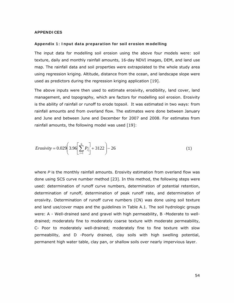
54
APPENDICES
Appendix 1: Input data preparation for soil erosion modelling
The input data for modelling soil erosion using the above four models were: soil
texture, daily and monthly rainfall amounts, 16-day NDVI images, DEM, and land use
map. The rainfall data and soil properties were extrapolated to the whole study area
using regression kriging. Altitude, distance from the ocean, and landscape slope were
used as predictors during the regression kriging application [19].
The above inputs were then used to estimate erosivity, erodibility, land cover, land
management, and topography, which are factors for modelling soil erosion. Erosivity
is the ability of rainfall or runoff to erode topsoil. It was estimated in two ways: from
rainfall amounts and from overland flow. The estimates were done between January
and June and between June and December for 2007 and 2008. For estimates from
rainfall amounts, the following model was used [19]:
26312296.3029.06
1−⎟⎟
⎠
⎞⎜⎜⎝
⎛+⎥
⎦
⎤⎢⎣
⎡= ∑
=iiPErosivity (1)
where P is the monthly rainfall amounts. Erosivity estimation from overland flow was
done using SCS curve number method [23]. In this method, the following steps were
used: determination of runoff curve numbers, determination of potential retention,
determination of runoff, determination of peak runoff rate, and determination of
erosivity. Determination of runoff curve numbers (CN) was done using soil texture
and land use/cover maps and the guidelines in Table A.1. The soil hydrologic groups
were: A - Well-drained sand and gravel with high permeability, B -Moderate to well-
drained; moderately fine to moderately coarse texture with moderate permeability,
C- Poor to moderately well-drained; moderately fine to fine texture with slow
permeability, and D -Poorly drained, clay soils with high swelling potential,
permanent high water table, clay pan, or shallow soils over nearly impervious layer.
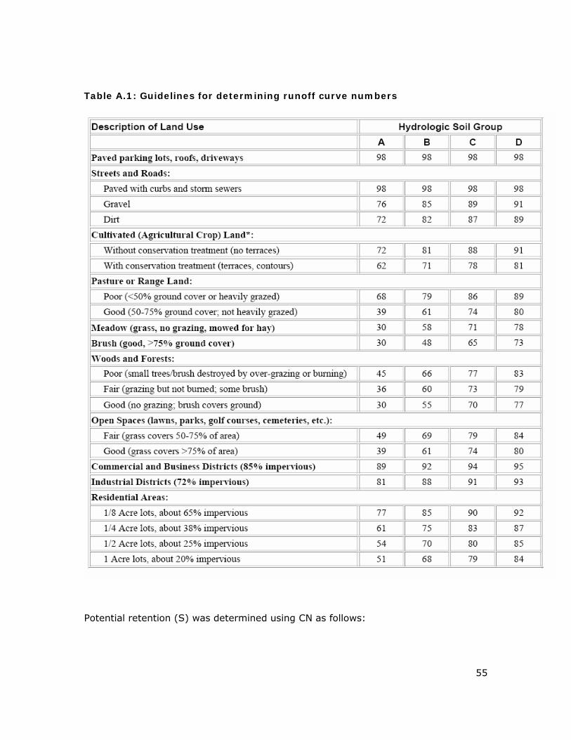
55
Table A.1: Guidelines for determining runoff curve numbers
Potential retention (S) was determined using CN as follows:
56
⎟⎠⎞
⎜⎝⎛ −= 1100254CN
S (2)
For example, around Marka town in the South of the study area, the land cover is
less than 50% on clay soil of poor drainage (hydrologic soil group D). Hence, the CN
= 89. Its potential retention using Equation (2) is 31.4.
Runoff amount was determined from the SCS equation as follows [23]:
( )( )
⎪⎪⎪
⎩
⎪⎪⎪
⎨
⎧
<
>+−
=
a
aa
i
IP
IPSP
IP
Runoff0
8.0
2
(3)
where Ia = 20% of retention potential S in Equation (2) and P is the daily rainfall
amount. In order to use the monthly rainfall data for the six-month duration, the
runoff estimate was summed for the six-month period using an exponential
relationship as shown in Equation (4), (5), (6), and (7) [34].
( ) [ ]mmmnA ii exp= (4)
mSmi Δ+= 2.0 (5)
Smm 2.0max −=Δ (6)
∑=
Δ=6
1**
iii AmrunoffRunoff (7)
where A is the rain-day frequency density, n is the number of rain days in the six-
month period, mmax is the maximum daily rainfall amount in the six-month duration,
and mi is the mean rainfall amount per day (intensity in amount/day). Erosivity from
the above runoff was then determined using Equation (8) and (9).
57
( ) 56.0**8.11 pQrunoffErosivity = (8)
( )017.0*903.0
16.07.0
4.25*_**97.3
pixel
prunofflengthpixelpixelQ ⎟
⎠⎞
⎜⎝⎛= (9)
where pixel is the area of the pixels in km2 and pixel_length is the length of the pixel
along the slope (m/km).
Soil erodibility was determined from soil texture as follows:
( )⎥⎥⎦
⎤
⎢⎢⎣
⎡ +−+=
57517.0519.1log
*5.0exp*00388.00035.02
gDyErodibilit (10)
where Dg is mean soil particle diameter and which is estimated by Equation (11)
[28].
⎥⎦
⎤⎢⎣
⎡= ∑
iiiig ddfD 21ln**01.0exp (11)
where fi is the particle fraction in percent, d1 is the maximum diameter (mm) of the
soil fraction, and d2 is the minimum diameter (mm) of the soil fraction. The inputs
for these estimations included fi from interpolated soil textural fractions, d1 taken as
2 mm for sand, 0.05 mm for silt, and 0.002 mm for clay, and d2 taken as 0.05 mm
for sand, 0.002 mm for silt, and 0.0005 mm for clay [28].
The land cover was determined using Equation (12).
⎟⎟⎠
⎞⎜⎜⎝
⎛−
−=NDVI
NDVIlandcβ
α *exp (12)
58
where landc is the land cover factor, NDVI is the mean NDVI from MODIS for the six-
month duration, α and β are constants taken as 2 and 1, respectively [19].
The land management factor represents the effect of soil and water conservation
practices for controlling loss of topsoil. Wischmeier and Smith [33] developed a
monograph for allocating indices to different land management. In this study, land
management practises were extracted from the land use map and assigned indices
according to Wischmeier and Smith [33] monograph.
The topographic factor of soil erosion was determined from slope and length of slope.
The length of slope was determined using Equation (13).
( )mmm
min
min
pixelApixelAL
)13.22(*)cossin(*2
112
αα +−+
= +
++
(13)
where Ain is the drainage contributing area at the inlet of a grid for which L is being
estimated, pixel is the DEM grid resolution, α is the flow direction within the grid, and
m is the exponent that addresses the ratio of rill-to-inter-rill soil loss. The value of m
was taken as 0.4 for slope angle St > 3°, 0.3 for 2° < St ≤ 3°, 0.2 for 1° < St ≤ 2°,
and 0.1 for St ≤ 1° [13]. The length of slope and slope were then combined to
produce slope-length factor which indexes topographic factor for soil erosion as
shown in Equation (14).
( )StStLLStm
2sin*41.65sin*56.4065.013.22
++⎟⎠⎞
⎜⎝⎛= (14)
where St is slope in degrees.
59
Appendix 2: Mineral glossary
Calcite: is a carbonate mineral and the most stable polymorph of calcium carbonate
(CaCO3). The other polymorphs are the minerals aragonite and vaterite.
Chlorites: is a group of phyllosilicate minerals. The typical general formula is:
(Mg,Fe)3(Si,Al)4O10(OH)2·(Mg,Fe)3(OH)6. This formula emphasises the structure of
the group.
Feldspar: is a huge family with very similar diffractometric properties. Chemical
formula is a-AlSi3O8 with a being either K, Na or Ca (in the latter case it will be
CaAl2Si2O8) .
Illite: is a non-expanding, clay-sized, micaceous mineral. Illite is a phyllosilicate or
layered alumino-silicate. The chemical formula is given as KyAl4(Si8y,Aly)O20(OH)4
usually with 1 < y < 1.5, but always with y < 2, but there is considerable ion
substitution.
Kaolinite: is a clay mineral with the chemical composition Al2Si2O5(OH)4. It is a
layered silicate mineral.
Quartz: is the most abundant mineral in the Earth's continental crust. It is made up
of a lattice of silica (SiO2) tetrahedral. Quartz is very hard (grade 7 on the Mohs
scale) and a density of 2.65 g/cm³.SiO2, density of 2.65 g/cm³.
Smectite: is a group of minerals including dioctahedral smectites such as
montmorillonite ((Na,Ca)0.33(Al,Mg)2Si4O10(OH)2nH2O) and nontronite
(Na0.3Fe2(Si,Al)4Si4O10(OH)2nH2O) and trioctahedral smectites for example saponite
(Ca0.25(Mg,Fe)3(Si,Al)4O10(OH)2nH2O).
ROCK GLOSSARY
Basalt: A dark, fine-grained, extrusive (volcanic) igneous rock with low silica content
(40% to 50%), but rich in iron, magnesium and calcium. Generally occurs in lava
flows, but also as dikes. Basalt makes up most of the ocean floor and is the most
abundant volcanic rock in the Earth’s crust.
Gneiss, Migmatite, Granulite: Gneiss is coarse-grained, foliated metamorphic rock
that commonly has alternating bands of light and dark-coloured minerals (gneiss).
Migmatites are metamorphic rock that are heated enough to partially melt, but not
60
completely. The molten minerals resolidify within the metamorphic rock, producing a
rock that incorporates both metamorphic and igneous features. Migmatites can also
form when metamorphic rock experiences multiple injections of igneous rock that
solidify to form a network of cross-cutting dikes (migmatite).
Granite: A coarse-grained intrusive igneous rock with at least 65% silica. Quartz,
plagioclase feldspar and potassium feldspar make up most of the rock and give it a
fairly light colour. Granite has more potassium feldspar than plagioclase feldspar.
Usually with biotite, but also may have hornblende.
Gypsum (or anhydrite,): It is the commonest sulphate mineral and is frequently
associated with halite and anhydrite in evaporites, forming thick, extensive beds
Limestone: A sedimentary rock made mostly of the mineral calcite (calcium
carbonate). Limestone is usually formed from shells of once-living organisms or
other organic processes, but may also form by inorganic precipitation.
Marbles: Marble is a metamorphic rock resulting from regional or rarely contact
metamorphism of sedimentary carbonate rocks, either limestone or dolomite rock, or
metamorphism of older marble. This metamorphic process causes a complete
recrystallization of the original rock into an interlocking mosaic of calcite, aragonite
and/or dolomite crystals. The temperatures and pressures necessary to form marble
usually destroy any fossils and sedimentary textures present in the original rock.
Marl and other mixtures: Consolidated and unconsolidated earthy deposits
consisting chiefly of an intimate mixture of clay and calcium carbonate, usually
including shell fragments and sometimes glauconite.
Rhyolite: Extrusive rock typically porphyritic and commonly it exhibits flow texture,
with phenocrystals of quartz and alkali feldspar in a glassy to cryptocrystalline
groundmass. It is an extrusive equivalent of granite (rhyolite).
Sandstone: Sedimentary rock made of sand-sized grains of different nature
Schist: Metamorphic rock usually derived from fine-grained sedimentary rock such
as shale. Individual minerals in schist have grown during metamorphism so that they
are easily visible to the naked eye. Schists are named for their mineral constituents.
For example, mica schist is conspicuously rich in mica such as biotite or muscovite.
Trachyte: is an igneous, volcanic rock with an aphanitic to porphyritic texture. The
mineral assemblage consists of essential alkali feldspar; relatively minor plagioclase

61
and quartz or a feldspathoid such as nepheline may also be present. (See the QAPF
diagram). Biotite, clinopyroxene and olivine are common accessory minerals.