Sections 6-1 and 6-2

Overview

Estimating a Population Proportion

INFERENTIAL STATISTICS

This chapter presents the beginnings of inferential statistics. The two major applications of inferential statistics involve the use of sample data to:

1. estimate the value of a population parameter, and

2. test some claim (or hypothesis) about a population.

INFERENTIAL STATISTICS (CONTINUED)

This chapter deals with the first of these.

1. We introduce methods for estimating values of these important population parameters: proportions and means.

2. We also present methods for determining sample sizes necessary to estimate those parameters.

ASSUMPTIONS FOR ESTIMATING A PROPORTION

We begin this chapter by estimating a population proportion. We make the following assumptions:

1. The sample is simple random.

2. The conditions for the binomial distribution are satisfied. (See Section 4-3.)

3. The normal distribution can be used to approximate the distribution of sample proportions because np ≥ 5 and nq ≥ 5 are

both satisfied.

NOTATION FOR PROPORTIONS

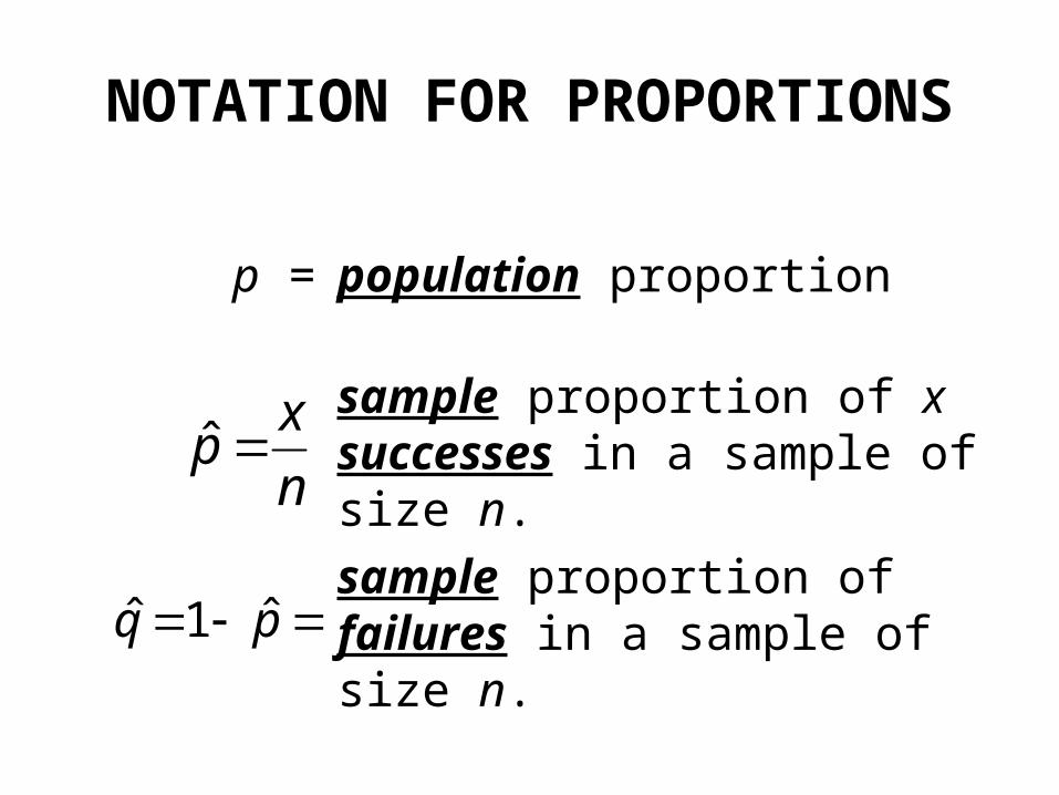
p = population proportion

sample proportion of x successes in a sample of size n.

sample proportion of failures in a sample of size n.

n

xp ˆ

pq ˆ1ˆ

POINT ESTIMATE

A point estimate is a single value (or point) used to approximate a population parameter.

The sample proportion is the best point estimate of the population proportion p.

p̂

CONFIDENCE INTERVALS

A confidence interval (or interval estimate) is a range (or an interval) of values used to estimate the true value of a population parameter. A confidence interval is sometimes abbreviated as CI.

CONFIDENCE LEVEL

A confidence level is the probability 1 − α (often expressed as the equivalent percentage value) that is the proportion of times that the confidence interval actually does contain the population parameter, assuming that the estimation process is repeated a large number of times. This is usually

90%, 95%, or 99%

(α = 10%) (α = 5%) (α = 1%)

CONFIDENCE LEVEL (CONCLUDED)

The confidence level is also called the degree of confidence or the confidence coefficient.

CRITICAL VALUES

1. Under certain conditions, the sampling distribution of sample proportions can be approximated by a normal distribution. (See Figure 6-2.)

2. Sample proportions have a relatively small chance (with probability denoted by α) of falling into one of the red tails of Figure 6 2.

3. Denoting the area of each shaded tail by α/2, we see that there is a total probability of α that a sample proportion will fall in either of the two red tails.

CRITICAL VALUES (CONCLUDED)

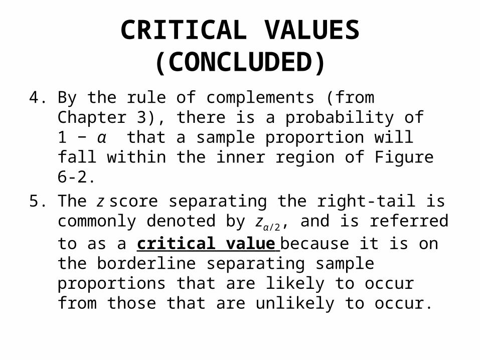
4. By the rule of complements (from Chapter 3), there is a probability of 1 − α that a sample proportion will fall within the inner region of Figure 6-2.

5. The z score separating the right-tail is commonly denoted by zα/2, and is referred to as a critical value because it is on the borderline separating sample proportions that are likely to occur from those that are unlikely to occur.

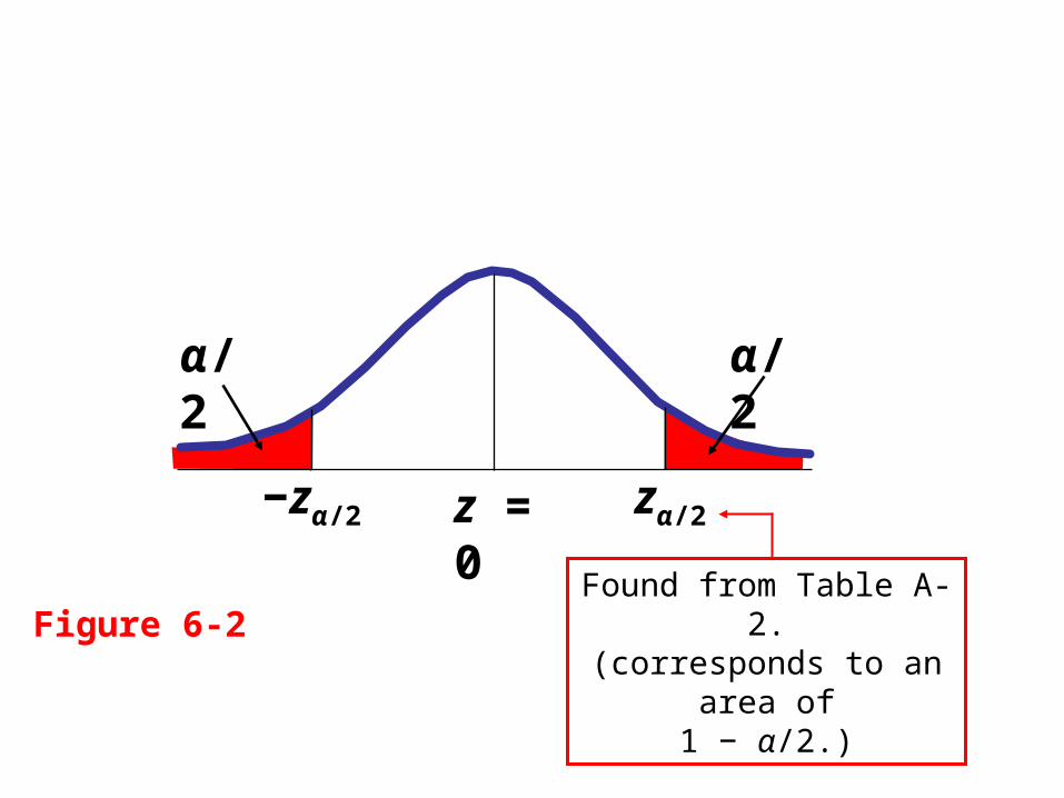
z = 0

Figure 6-2Found from Table A-2.

(corresponds to an area of1 − α/2.)

−zα/2 zα/2

α/2 α/2

CRITICAL VALUE

A critical value is the number on the borderline separating sample statistics that are likely to occur from those that are unlikely to occur. The number zα/2 is a critical value that is a z score with the property that it separates an area of α/2 in the right tail of the standard normal distribution. (See Figure 6-2).

NOTATION FOR CRITICAL VALUE

The critical value zα/2 is the positive z value that is at the vertical boundary separating an area of α/2 in the right tail of the standard normal distribution. (The value of –zα/2 is at the vertical boundary for the area of α/2 in the left tail). The subscript α/2 is simply a reminder that the z score separates an area of α/2 in the right tail of the standard normal distribution.

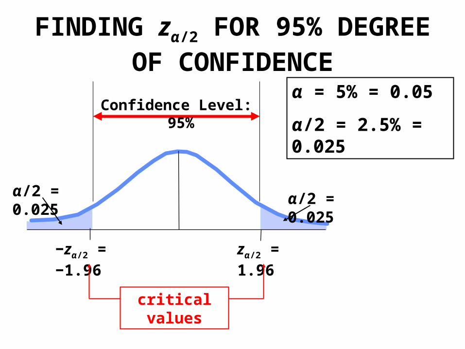
FINDING zα/2 FOR 95% DEGREE OF CONFIDENCE

−zα/2 = −1.96 zα/2 = 1.96

α = 5% = 0.05

α/2 = 2.5% = 0.025

α/2 = 0.025α/2 = 0.025

Confidence Level: 95%

critical values

MARGIN FOR ERROR

When data from a simple random sample are used to estimate a population proportion p, the margin of error, denoted by E, is the maximum likely (with probability 1 – α) difference between the observed proportion p and the true value of the population proportion p.

ˆ

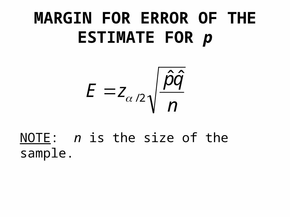
MARGIN FOR ERROR OF THE ESTIMATE FOR p

n

qpzE

ˆˆ2/

NOTE: n is the size of the sample.

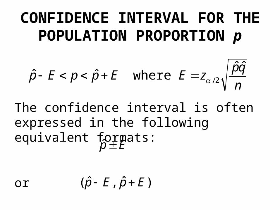
The confidence interval is often expressed in the following equivalent formats:

or

CONFIDENCE INTERVAL FOR THE POPULATION PROPORTION p

n

qpzEEppEp

ˆˆwhereˆˆ 2/

)ˆ,ˆ(

ˆ

EpEp

Ep

ROUND-OFF RULE FOR CONFIDENCE INTERVALS

Round the confidence interval limits to

three significant digits.

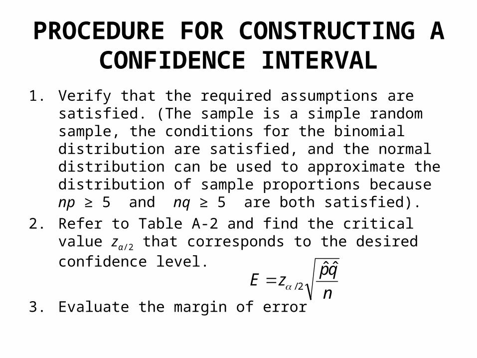
PROCEDURE FOR CONSTRUCTING A CONFIDENCE INTERVAL

1. Verify that the required assumptions are satisfied. (The sample is a simple random sample, the conditions for the binomial distribution are satisfied, and the normal distribution can be used to approximate the distribution of sample proportions because np ≥ 5 and nq ≥ 5 are both satisfied).

2. Refer to Table A-2 and find the critical value zα/2 that corresponds to the desired confidence level.

3. Evaluate the margin of errorn

qpzE

ˆˆ2/

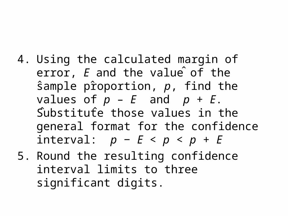
4. Using the calculated margin of error, E and the value of the sample proportion, p, find the values of p – E and p + E. Substitute those values in the general format for the confidence interval: p − E < p < p + E

5. Round the resulting confidence interval limits to three significant digits.

ˆ ˆ

ˆˆˆ

CONFIDENCE INTERVAL LIMITS

The two values are called confidence interval limits.

EpEp ˆandˆ

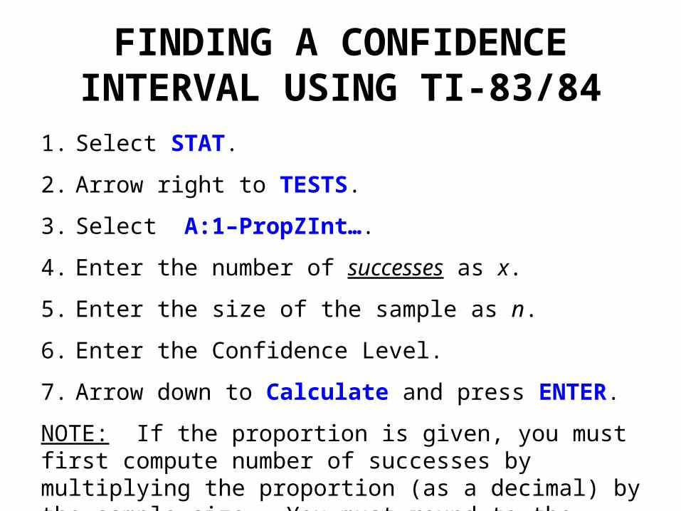
FINDING A CONFIDENCE INTERVAL USING TI-83/84

1. Select STAT.

2. Arrow right to TESTS.

3. Select A:1–PropZInt….

4. Enter the number of successes as x.

5. Enter the size of the sample as n.

6. Enter the Confidence Level.

7. Arrow down to Calculate and press ENTER.

NOTE: If the proportion is given, you must first compute number of successes by multiplying the proportion (as a decimal) by the sample size. You must round to the nearest integer.

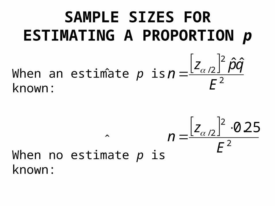
SAMPLE SIZES FOR ESTIMATING A PROPORTION p

When an estimate p is known:

When no estimate p is known:

ˆ

ˆ

2

22/

2

22/

25.0

ˆˆ

E

zn

E

qpzn

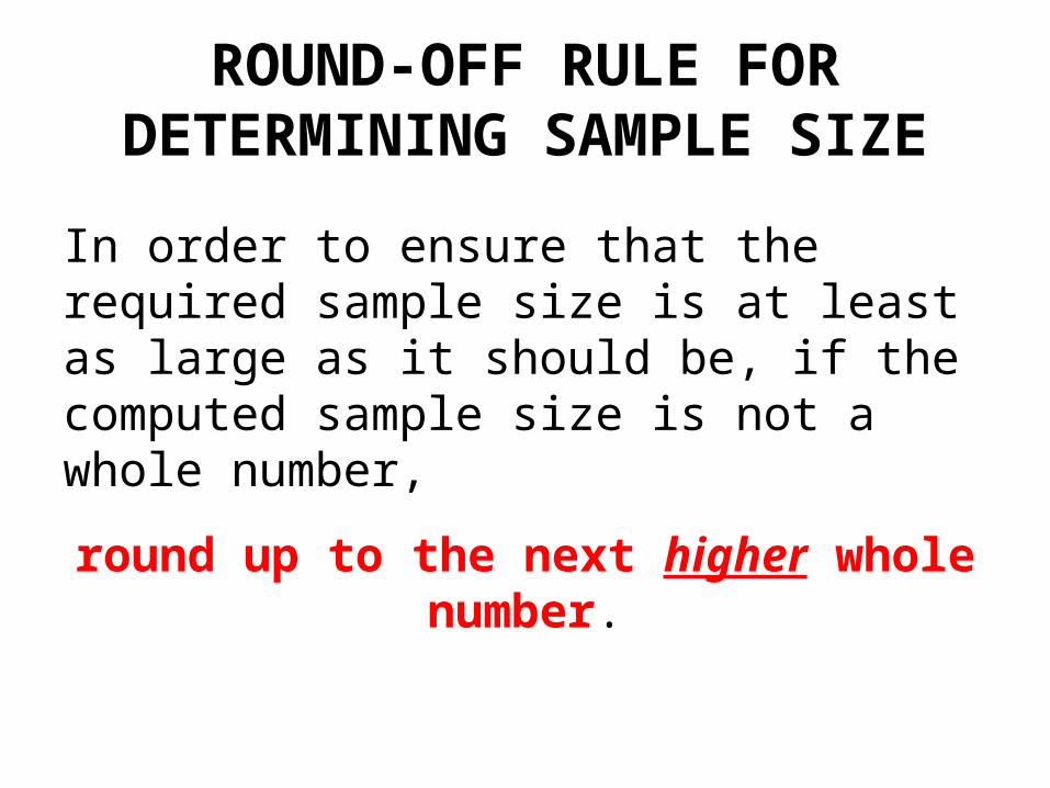
ROUND-OFF RULE FOR DETERMINING SAMPLE SIZE

In order to ensure that the required sample size is at least as large as it should be, if the computed sample size is not a whole number,

round up to the next higher whole number.

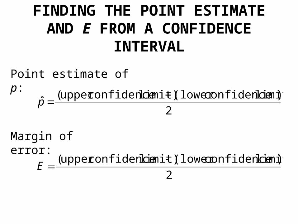
FINDING THE POINT ESTIMATE AND E FROM A CONFIDENCE INTERVAL

2

)limitconfidence(lowerlimit)confidenceupper(

2

)limitconfidence(lowerlimit)confidenceupper(ˆ

E

p

Point estimate of p:

Margin of error: