Section1: Introduction,ProbabilityConcepts andDecisions · CourseOverview Section 1: Introduction,ProbabilityConceptsandDecisions Section 2: LearningfromData: Estimation,ConﬁdenceIntervals

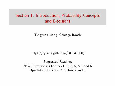
Section 1: Introduction, Probability Conceptsand Decisions

Tengyuan Liang, Chicago Booth

https://tyliang.github.io/BUS41000/

Suggested Reading:Naked Statistics, Chapters 1, 2, 3, 5, 5.5 and 6

OpenIntro Statistics, Chapters 2 and 3

https://tyliang.github.io/BUS41000/

Getting Started

I SyllabusI General Expectations

1. Read the notes2. Work on homework assignments3. Be on schedule

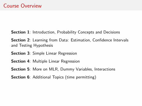
Course Overview

Section 1: Introduction, Probability Concepts and Decisions

Section 2: Learning from Data: Estimation, Confidence Intervalsand Testing Hypothesis

Section 3: Simple Linear Regression

Section 4: Multiple Linear Regression

Section 5: More on MLR, Dummy Variables, Interactions

Section 6: Additional Topics (time permitting)

Course Schedule

Week 1 Section 1

Week 2 Section 1

Week 3 Section 2

Week 4 Section 2

Week 5 Section 3

Week 6 Section 3 and Review

Week 7 Midterm

Week 8 Section 4

Week 9 Section 5

Week 10 Section 6 and Review

Finals Week Final

Let’s start with a question. . .

My entire portfolio is in U.S. equities. How would you describe thepotential outcomes for my returns in 2018?

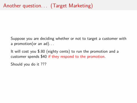
Another question. . . (Target Marketing)

Suppose you are deciding whether or not to target a customer witha promotion(or an ad). . .

It will cost you $.80 (eighty cents) to run the promotion and acustomer spends $40 if they respond to the promotion.

Should you do it ???

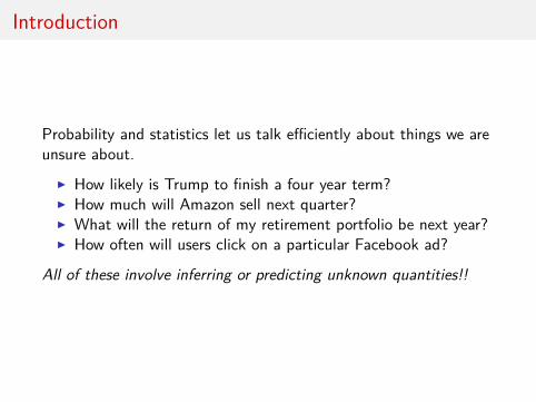
Introduction

Probability and statistics let us talk efficiently about things we areunsure about.

I How likely is Trump to finish a four year term?I How much will Amazon sell next quarter?I What will the return of my retirement portfolio be next year?I How often will users click on a particular Facebook ad?

All of these involve inferring or predicting unknown quantities!!

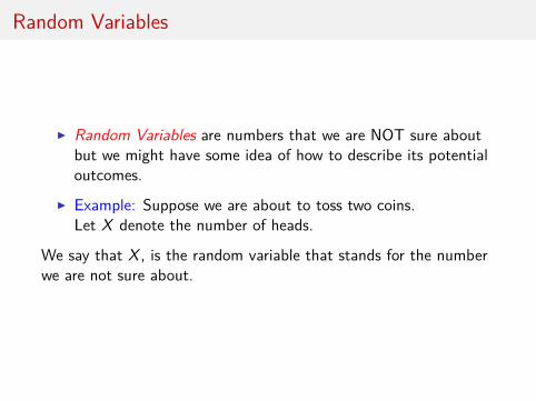
Random Variables

I Random Variables are numbers that we are NOT sure aboutbut we might have some idea of how to describe its potentialoutcomes.

I Example: Suppose we are about to toss two coins.Let X denote the number of heads.

We say that X , is the random variable that stands for the numberwe are not sure about.

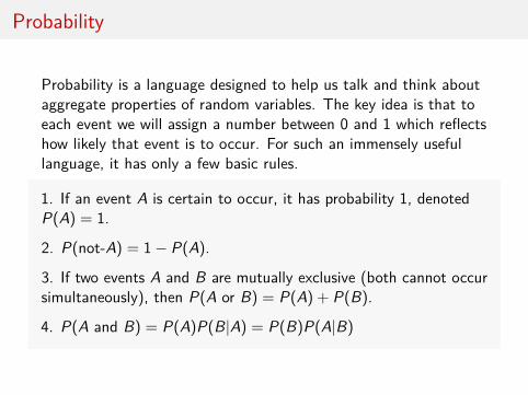
Probability

Probability is a language designed to help us talk and think aboutaggregate properties of random variables. The key idea is that toeach event we will assign a number between 0 and 1 which reflectshow likely that event is to occur. For such an immensely usefullanguage, it has only a few basic rules.

1. If an event A is certain to occur, it has probability 1, denotedP(A) = 1.

2. P(not-A) = 1− P(A).

3. If two events A and B are mutually exclusive (both cannot occursimultaneously), then P(A or B) = P(A) + P(B).

4. P(A and B) = P(A)P(B|A) = P(B)P(A|B)

Probability Distribution

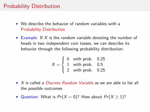
I We describe the behavior of random variables with aProbability Distribution

I Example: If X is the random variable denoting the number ofheads in two independent coin tosses, we can describe itsbehavior through the following probability distribution:

X =

0 with prob. 0.251 with prob. 0.52 with prob. 0.25

I X is called a Discrete Random Variable as we are able to list allthe possible outcomes

I Question: What is Pr(X = 0)? How about Pr(X ≥ 1)?

Pete Rose Hitting Streak

Pete Rose of the Cincinnati Reds set a National League record ofhitting safely in 44 consecutive games. . .

I Rose was a 300 hitter.

I Assume he comes to bat 4 times each game.

I Each at bat is assumed to be independent, i.e., the current atbat doesn’t affect the outcome of the next.

What probability might reasonably be associated with a hittingstreak of that length?

Pete Rose Hitting Streak

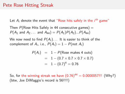
Let Ai denote the event that “Rose hits safely in the i th game”

Then P(Rose Hits Safely in 44 consecutive games) =P(A1 and A2 . . . and A44) = P(A1)P(A2)...P(A44)

We now need to find P(Ai). . . It is easier to think of thecomplement of Ai , i.e., P(Ai) = 1− P(not Ai)

P(Ai) = 1− P(Rose makes 4 outs)= 1− (0.7× 0.7× 0.7× 0.7)= 1− (0.7)4 = 0.76

So, for the winning streak we have (0.76)44 = 0.0000057!!! (Why?)(btw, Joe DiMaggio’s record is 56!!!!)

New England Patriots and Coin Tosses

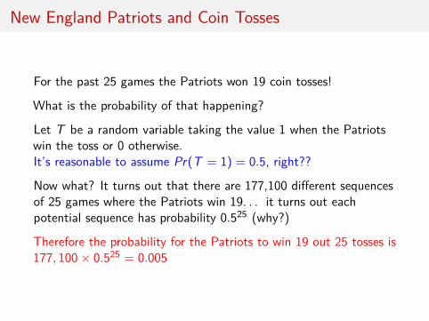
For the past 25 games the Patriots won 19 coin tosses!

What is the probability of that happening?

Let T be a random variable taking the value 1 when the Patriotswin the toss or 0 otherwise.It’s reasonable to assume Pr(T = 1) = 0.5, right??

Now what? It turns out that there are 177,100 different sequencesof 25 games where the Patriots win 19. . . it turns out eachpotential sequence has probability 0.525 (why?)

Therefore the probability for the Patriots to win 19 out 25 tosses is177, 100× 0.525 = 0.005

Conditional, Joint and Marginal Distributions

In general we want to use probability to address problems involvingmore than one variable at the time

Think back to our first question on the returns of my portfolio... ifwe know that the economy will be growing next year, does thatchange the assessment about the behavior of my returns?

We need to be able to describe what we think will happen to onevariable relative to another. . .


Here’s an example: we want to answer questions like: How are mysales impacted by the overall economy?

Let E denote the performance of the economy next quarter. . . forsimplicity, say E = 1 if the economy is expanding and E = 0 if theeconomy is contracting (what kind of random variable is this?)Let’s assume pr(E = 1) = 0.7


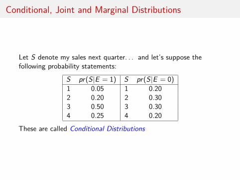
Let S denote my sales next quarter. . . and let’s suppose thefollowing probability statements:

S pr(S|E = 1) S pr(S|E = 0)1 0.05 1 0.202 0.20 2 0.303 0.50 3 0.304 0.25 4 0.20

These are called Conditional Distributions


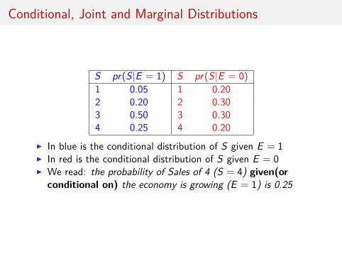
S pr(S|E = 1) S pr(S|E = 0)1 0.05 1 0.202 0.20 2 0.303 0.50 3 0.304 0.25 4 0.20

I In blue is the conditional distribution of S given E = 1I In red is the conditional distribution of S given E = 0I We read: the probability of Sales of 4 (S = 4) given(or

conditional on) the economy is growing (E = 1) is 0.25


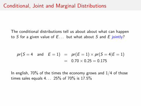
The conditional distributions tell us about about what can happento S for a given value of E . . . but what about S and E jointly?

pr(S = 4 and E = 1) = pr(E = 1)× pr(S = 4|E = 1)= 0.70× 0.25 = 0.175

In english, 70% of the times the economy grows and 1/4 of thosetimes sales equals 4. . . 25% of 70% is 17.5%


>IJP37Q

>IKP&$6%Q

AIX

AI

AIW

AIJ

AIX

AI

AIW

AIJ

/0

/1

/2

/2

/1

/1

/23

/3

/2

/43

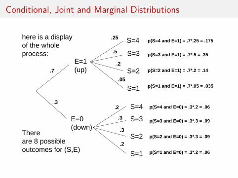
5"#$%&'()&*$+,&$&/0-/23&$&/+03&

5"#$1&'()&*$+,&$&/0-/3&$&/13

5"#$2&'()&*$+,&$&/0-/2&$&/+%&

5"#$+&'()&*$+,&$&/0-/43&$&/413&

5"#$%&'()&*$4,&$&/1-/2&$&/46

5"#$1&'()&*$4,&$&/1-/1 $&/47

5"#$2&'()&*$4,&$&/1-/1 $&/47

5"#$+&'()&*$4,&$&/1-/2&$&/46

49)("'1"(95"'()*"#(% ]PAIXQ"M

95.5"'1")"&'17*)8$B"(95"69$*57.$<511@

N95.5").5"^"7$11'2*5$3(<$=51"B$."PA+>Q

!JRV_!K`


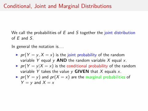
We call the probabilities of E and S together the joint distributionof E and S.

In general the notation is. . .

I pr(Y = y ,X = x) is the joint probability of the randomvariable Y equal y AND the random variable X equal x .

I pr(Y = y |X = x) is the conditional probability of the randomvariable Y takes the value y GIVEN that X equals x .

I pr(Y = y) and pr(X = x) are the marginal probabilities ofY = y and X = x


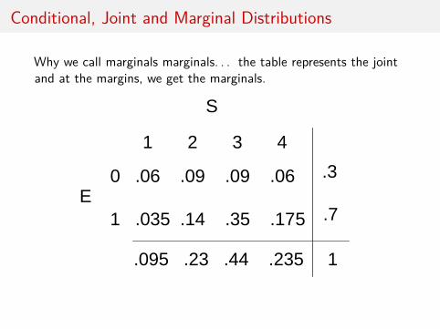
Why we call marginals marginals. . . the table represents the jointand at the margins, we get the marginals.

>?)=7*5"A")%&">")/)'%

45"<)%"&'17*)8"(95"a$'%("&'1(.'23('$%"$B"A")%&">"31'%/)"(6$"6)8"()2*5!

N95"5%(.8"'%"(95"1"<$*3=%")%&"5".$6"/';51"]PAI1")%&">I5Q!

A

J"""""""W""""""" """""""X

>K"""!K`""""!Kb""""!Kb !K`

J"""!K V""!JX""""! V""""!JRV

!

!R

!KbV"""!W """!XX""""!W V J

T$6"8$3"<)%155"698"(95=)./'%)*1).5"<)**5&(95"=)./'%)*1!


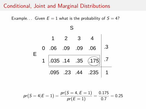
Example. . . Given E = 1 what is the probability of S = 4?

A

J"""""""W""""""" """""""X

>K"""!K`""""!Kb""""!Kb !K`

J"""!K V""!JX""""! V""""!JRV

!

!R

!KbV"""!W """!XX""""!W V J

>?)=7*5

! !"# ! $#! "

7PA +> Q !7PA U> Q !

7P> Q !

i';5%">"3769)("'1"(957.$2 A)*51IXM

PB.$="(95"a$'%(&'1(.'23('$%Q

pr(S = 4|E = 1) = pr(S = 4,E = 1)pr(E = 1) = 0.175

0.7 = 0.25


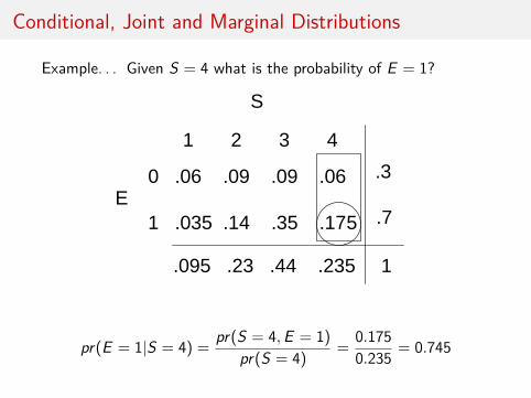
Example. . . Given S = 4 what is the probability of E = 1?

A

J"""""""W""""""" """""""X

>K"""!K`""""!Kb""""!Kb !K`

J"""!K V""!JX""""! V""""!JRV

!

!R

!KbV"""!W """!XX""""!W V J

! !"#! " # $%#

7PA +> Q !7P> U A Q !

7PA Q !

i';5%"1)*51IX+69)("'1"(957.$2)2'*'(8(95%">"'1"37M

pr(E = 1|S = 4) = pr(S = 4,E = 1)pr(S = 4) = 0.175

0.235 = 0.745

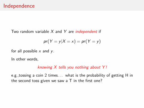
Independence

Two random variable X and Y are independent if

pr(Y = y |X = x) = pr(Y = y)

for all possible x and y .

In other words,

knowing X tells you nothing about Y !

e.g.,tossing a coin 2 times. . . what is the probability of getting H inthe second toss given we saw a T in the first one?

Trump’s victory

Let’s try to figure out why were people so confused on November8th 2016. . .

I am simplifying things a bit, but starting the day, Trump had to win5 states to get the presidency: Florida, North Carolina,Pennsylvania, Michigan and Wisconsin. One could also say thateach of these states had a 50-50 change for Trump and Hillary.

So, based on this information, what was the probability of a Trumpvictory? (Homework: make sure to revisit this at home. )

[FiveThirtyEight article on 2016 election, further reading]

http://fivethirtyeight.com/features/why-fivethirtyeight-gave-trump-a-better-chance-than-almost-anyone-else/

Disease Testing Example

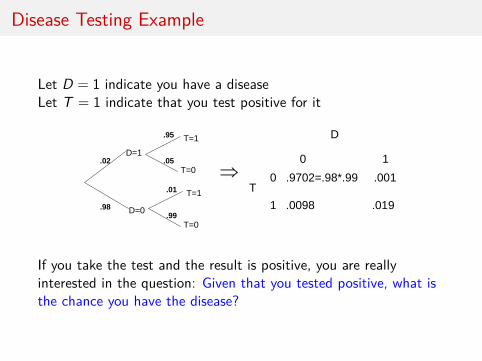
Let D = 1 indicate you have a diseaseLet T = 1 indicate that you test positive for it

>?)=7*5

0'15)15"(51('%/!

H5("0"IJ"'%&'<)(5"8$3"9);5"(95"&'15)15!H5("NIJ"'%&'<)(5"(9)("8$3"(51("7$1'(';5"B$."'(!

-$1("&$<($.1"(9'%:"'%"(5.=1"$B"7P&Q")%&"7P(U&Q!

/42

/7G

0IJ

0IK

NIJ

NIK

/73

/43

NIJ

NIK

/4+

/77

"

0

K""""""""""""""""""""""""J

NK"""!bRKWI!b^Z!bb"""""!KKJ

J"""!KKb^""""""""""""""""""!KJb

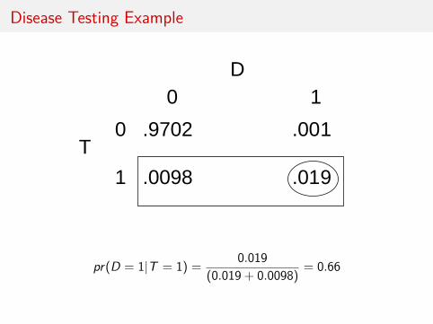
If you take the test and the result is positive, you are reallyinterested in the question: Given that you tested positive, what isthe chance you have the disease?

Disease Testing Example

F3("'B"8$3").5"(95"7)('5%("69$"(51(1"7$1'(';5"B$.)"&'15)15"8$3"<).5")2$3("]P0IJUNIJQ"P7P&U(QQ!

0K""""""""""""""""""""""""J

NK"""!bRKW""""""""""""""""""!KKJ

J"""!KKb^""""""""""""""""""!KJb

]P0IJUNIJQ"I"!KJb¥P!KJb_!KKb^Q"I"K!``

+,"-.#/&!0/$.1$/2!1"$"-.3/45($61/$5./75(#7./&!05(-./$5./8"1.(1.9+

pr(D = 1|T = 1) = 0.019(0.019 + 0.0098) = 0.66

Bayes Theorem (aside)

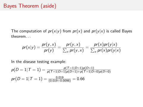
The computation of pr(x |y) from pr(x) and pr(y |x) is called Bayestheorem. . .

pr(x |y) = pr(y , x)pr(y) = pr(y , x)∑

x pr(y , x) = pr(x)pr(y |x)∑x pr(x)pr(y |x)

In the disease testing example:

p(D = 1|T = 1) = p(T=1|D=1)p(D=1)p(T=1|D=1)p(D=1)+p(T=1|D=0)p(D=0)

pr(D = 1|T = 1) = 0.019(0.019+0.0098) = 0.66

Bayes Theorem (aside)

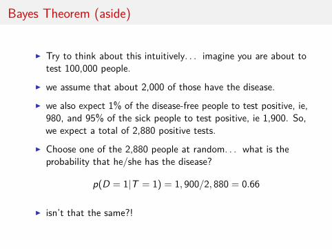
I Try to think about this intuitively. . . imagine you are about totest 100,000 people.

I we assume that about 2,000 of those have the disease.

I we also expect 1% of the disease-free people to test positive, ie,980, and 95% of the sick people to test positive, ie 1,900. So,we expect a total of 2,880 positive tests.

I Choose one of the 2,880 people at random. . . what is theprobability that he/she has the disease?

p(D = 1|T = 1) = 1, 900/2, 880 = 0.66

I isn’t that the same?!

Probability and Decisions

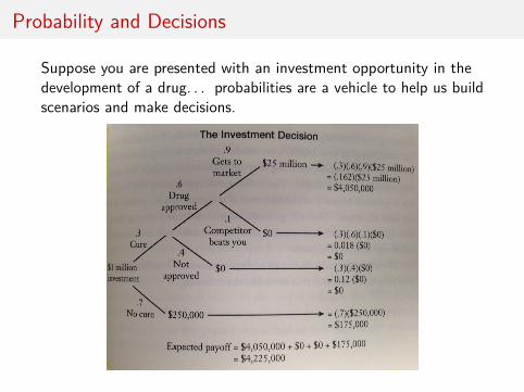
Suppose you are presented with an investment opportunity in thedevelopment of a drug. . . probabilities are a vehicle to help us buildscenarios and make decisions.


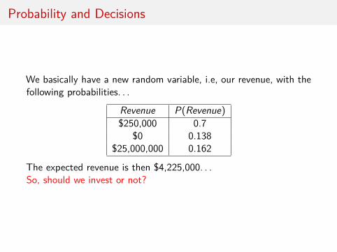
We basically have a new random variable, i.e, our revenue, with thefollowing probabilities. . .

Revenue P(Revenue)$250,000 0.7

$0 0.138$25,000,000 0.162

The expected revenue is then $4,225,000. . .So, should we invest or not?

Back to Target Marketing

Should we send the promotion ???

Well, it depends on how likely it is that the customer will respond!!

If they respond, you get 40-0.8=$39.20.

If they do not respond, you lose $0.80.

Let’s assume your “predictive analytics” team has studied theconditional probability of customer responses given customercharacteristics. . . (say, previous purchase behavior, demographics,etc)

Back to Target Marketing

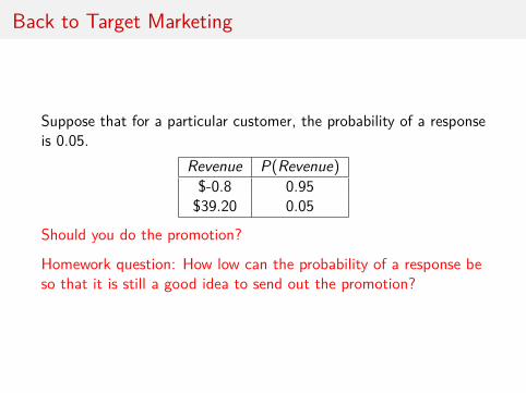
Suppose that for a particular customer, the probability of a responseis 0.05.

Revenue P(Revenue)$-0.8 0.95$39.20 0.05

Should you do the promotion?

Homework question: How low can the probability of a response beso that it is still a good idea to send out the promotion?


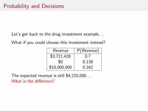
Let’s get back to the drug investment example. . .

What if you could choose this investment instead?

Revenue P(Revenue)$3,721,428 0.7

$0 0.138$10,000,000 0.162

The expected revenue is still $4,225,000. . .What is the difference?

Mean and Variance of a Random Variable

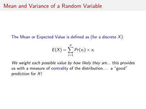
The Mean or Expected Value is defined as (for a discrete X ):

E (X ) =n∑

i=1Pr(xi)× xi

We weight each possible value by how likely they are... this providesus with a measure of centrality of the distribution. . . a “good”prediction for X !


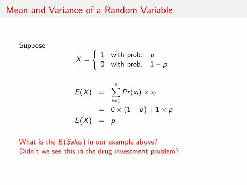
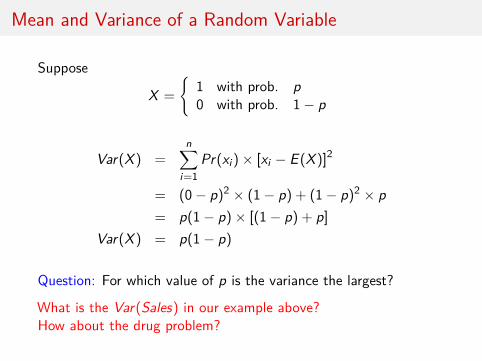
Suppose

X ={

1 with prob. p0 with prob. 1− p

E (X ) =n∑

i=1Pr(xi)× xi

= 0× (1− p) + 1× pE (X ) = p

What is the E (Sales) in our example above?Didn’t we see this in the drug investment problem?


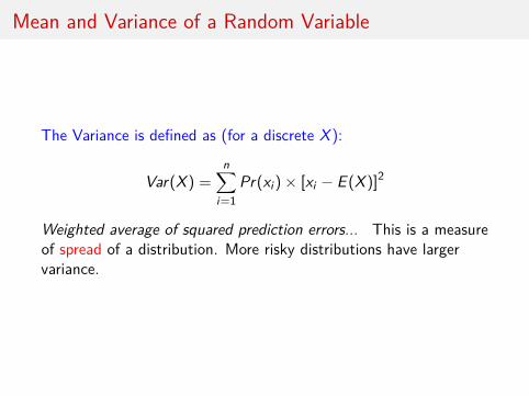
The Variance is defined as (for a discrete X ):

Var(X ) =n∑

i=1Pr(xi)× [xi − E (X )]2

Weighted average of squared prediction errors... This is a measureof spread of a distribution. More risky distributions have largervariance.


Suppose

X ={

1 with prob. p0 with prob. 1− p

Var(X ) =n∑

i=1Pr(xi)× [xi − E (X )]2

= (0− p)2 × (1− p) + (1− p)2 × p= p(1− p)× [(1− p) + p]

Var(X ) = p(1− p)

Question: For which value of p is the variance the largest?

What is the Var(Sales) in our example above?How about the drug problem?

The Standard Deviation

I What are the units of E (X )? What are the units of Var(X )?

I A more intuitive way to understand the spread of a distributionis to look at the standard deviation:

sd(X ) =√Var(X )

I What are the units of sd(X )?

Covariance

I A measure of dependence between two random variables. . .

I It tells us how two unknown quantities tend to move together

The Covariance is defined as (for discrete X and Y ):

Cov(X ,Y ) =n∑

i=1

m∑j=1

Pr(xi , yj)× [xi − E (X )]× [yj − E (Y )]

I What are the units of Cov(X ,Y ) ?

I What is the Cov(Sales,Economy) in our example above?

Ford vs. Tesla

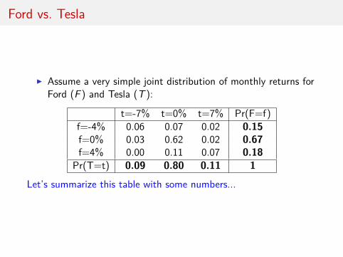
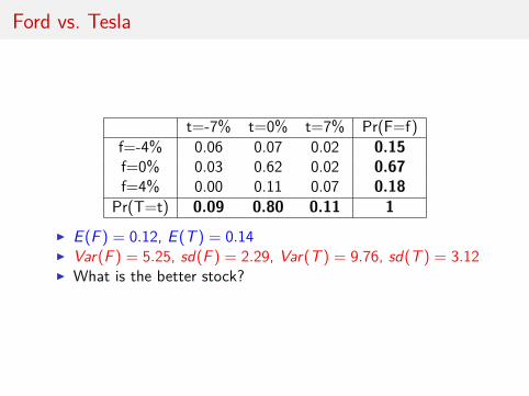
I Assume a very simple joint distribution of monthly returns forFord (F ) and Tesla (T ):

t=-7% t=0% t=7% Pr(F=f)f=-4% 0.06 0.07 0.02 0.15f=0% 0.03 0.62 0.02 0.67f=4% 0.00 0.11 0.07 0.18

Pr(T=t) 0.09 0.80 0.11 1

Let’s summarize this table with some numbers...

Ford vs. Tesla

t=-7% t=0% t=7% Pr(F=f)f=-4% 0.06 0.07 0.02 0.15f=0% 0.03 0.62 0.02 0.67f=4% 0.00 0.11 0.07 0.18

Pr(T=t) 0.09 0.80 0.11 1

I E (F ) = 0.12, E (T ) = 0.14I Var(F ) = 5.25, sd(F ) = 2.29, Var(T ) = 9.76, sd(T ) = 3.12I What is the better stock?

Ford vs. Tesla

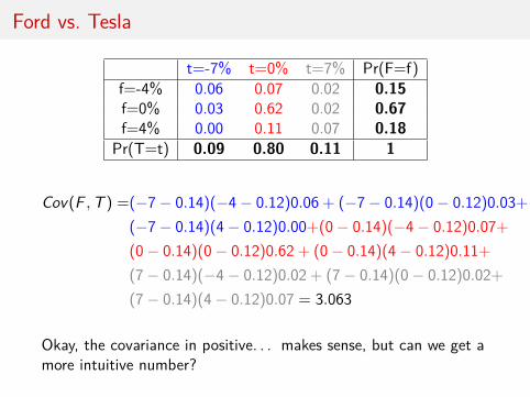
t=-7% t=0% t=7% Pr(F=f)f=-4% 0.06 0.07 0.02 0.15f=0% 0.03 0.62 0.02 0.67f=4% 0.00 0.11 0.07 0.18

Pr(T=t) 0.09 0.80 0.11 1

Cov(F ,T ) =(−7− 0.14)(−4− 0.12)0.06 + (−7− 0.14)(0− 0.12)0.03+(−7− 0.14)(4− 0.12)0.00+(0− 0.14)(−4− 0.12)0.07+(0− 0.14)(0− 0.12)0.62 + (0− 0.14)(4− 0.12)0.11+(7− 0.14)(−4− 0.12)0.02 + (7− 0.14)(0− 0.12)0.02+(7− 0.14)(4− 0.12)0.07 = 3.063

Okay, the covariance in positive. . . makes sense, but can we get amore intuitive number?

Correlation

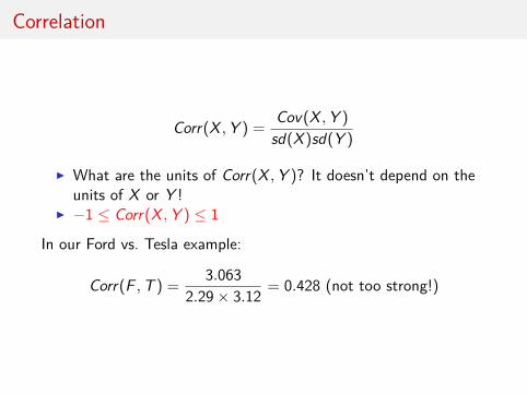
Corr(X ,Y ) = Cov(X ,Y )sd(X )sd(Y )

I What are the units of Corr(X ,Y )? It doesn’t depend on theunits of X or Y !

I −1 ≤ Corr(X ,Y ) ≤ 1

In our Ford vs. Tesla example:

Corr(F ,T ) = 3.0632.29× 3.12 = 0.428 (not too strong!)

Linear Combination of Random Variables

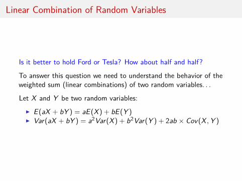
Is it better to hold Ford or Tesla? How about half and half?

To answer this question we need to understand the behavior of theweighted sum (linear combinations) of two random variables. . .

Let X and Y be two random variables:

I E (aX + bY ) = aE (X ) + bE (Y )I Var(aX + bY ) = a2Var(X ) + b2Var(Y ) + 2ab × Cov(X ,Y )


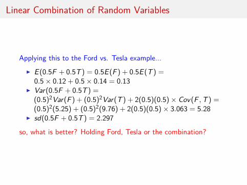
Applying this to the Ford vs. Tesla example...

I E (0.5F + 0.5T ) = 0.5E (F ) + 0.5E (T ) =0.5× 0.12 + 0.5× 0.14 = 0.13

I Var(0.5F + 0.5T ) =(0.5)2Var(F ) + (0.5)2Var(T ) + 2(0.5)(0.5)× Cov(F ,T ) =(0.5)2(5.25) + (0.5)2(9.76) + 2(0.5)(0.5)× 3.063 = 5.28

I sd(0.5F + 0.5T ) = 2.297

so, what is better? Holding Ford, Tesla or the combination?


More generally. . .

I E (w1X1 + w2X2 + ...wpXp) =w1E (X1) + w2E (X2) + ...+ wpE (Xp) =

∑pi=1 wiE (Xi)

I Var(w1X1 +w2X2 + ...wpXp) = w21Var(X1) +w2

2Var(X2) + ...+w2

pVar(Xp)+2w1w2×Cov(X1,X2)+2w1w3Cov(X1,X3)+ ... =∑pi=1 w2

i Var(Xi) +∑p

i=1∑

j 6=i wiwjCov(Xi ,Xj)

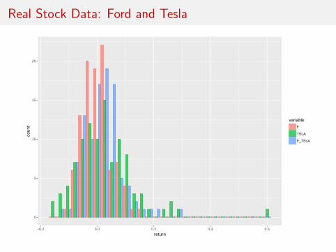
Real Stock Data: Ford and Tesla

0

5

10

15

20

−0.2 0.0 0.2 0.4 0.6

return

coun

t

variable

F

TSLA

F_TSLA

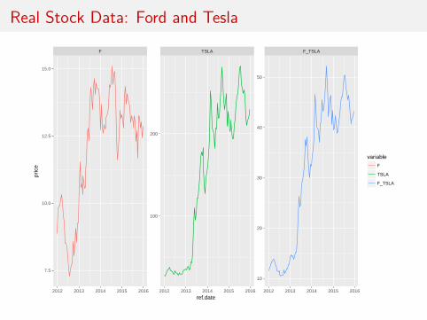
Real Stock Data: Ford and Tesla

F TSLA F_TSLA

2012 2013 2014 2015 2016 2012 2013 2014 2015 2016 2012 2013 2014 2015 2016

10

20

30

40

50

100

200

7.5

10.0

12.5

15.0

ref.date

pric

e

variable

F

TSLA

F_TSLA

Portfolio vs. Single Project (from Misbehaving)

In a meeting with 23 executives plus the CEO of a major companyeconomist Richard Thaler poses the following question:

Suppose you were offered an investment opportunity for yourdivision (each executive headed a separate/independent division)that will yield one of two payoffs. After the investment is made,there is a 50% chance it will make a profit of $2 million, and a 50%chance it will lose $1 million. Thaler then asked by a show of handswho of the executives would take on this project. Of thetwenty-three executives, only three said they would do it.

Anything wrong with that?


Then Thaler asked the CEO a question. If these projects wereindependent, that is, the success of one was unrelated to thesuccess of another, how many of the projects would he want toundertake? His answer: all of them! By taking on twenty threeprojects, the firm expects to make $11.5 million (since each of themis worth an expected half million), and a bit of mathematics revealsthat the chance of losing any money overall is less than 10%.(Homework: why? trick one... dont worry too much about it...)

Homework: compare the “sharpe ratio” of a single project vs.taking on all the projects


Companies, CEO’s, managers have to be careful in settingincentives that avoid what psychologist and behavior economists call“narrow framing”. . . otherwise, what can be perceived to be bad forone manager may be very good for the entire company!

Continuous Random Variables

I Suppose we are trying to predict tomorrow’s return on theS&P500. . .

I Question: What is the random variable of interest?I Question: How can we describe our uncertainty about

tomorrow’s outcome?I Listing all possible values seems like a crazy task. . . we’ll work

with intervals instead.I These are call continuous random variables.I The probability of an interval is defined by the area under the

probability density function.

The Normal Distribution

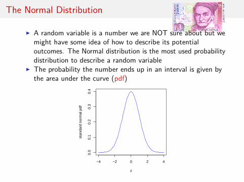
I A random variable is a number we are NOT sure about but wemight have some idea of how to describe its potentialoutcomes. The Normal distribution is the most used probabilitydistribution to describe a random variable

I The probability the number ends up in an interval is given bythe area under the curve (pdf)

−4 −2 0 2 4

0.0

0.1

0.2

0.3

0.4

z

stan

dard

nor

mal

pdf

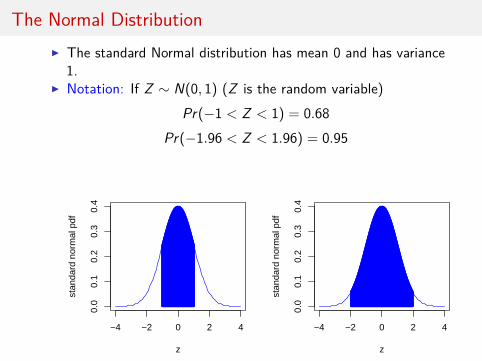
The Normal DistributionI The standard Normal distribution has mean 0 and has variance

1.I Notation: If Z ∼ N(0, 1) (Z is the random variable)

Pr(−1 < Z < 1) = 0.68Pr(−1.96 < Z < 1.96) = 0.95

−4 −2 0 2 4

0.0

0.1

0.2

0.3

0.4

z

stan

dard

nor

mal

pdf

−4 −2 0 2 4

0.0

0.1

0.2

0.3

0.4

z

stan

dard

nor

mal

pdf


Note:

For simplicity we will often use P(−2 < Z < 2) ≈ 0.95

Questions:

I What is Pr(Z < 2) ? How about Pr(Z ≤ 2)?I What is Pr(Z < 0)?


I The standard normal is not that useful by itself. When we say“the normal distribution”, we really mean a family ofdistributions.

I We obtain pdfs in the normal family by shifting the bell curvearound and spreading it out (or tightening it up).

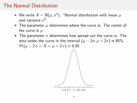
The Normal DistributionI We write X ∼ N(µ, σ2). “Normal distribution with mean µ

and variance σ2.I The parameter µ determines where the curve is. The center of

the curve is µ.I The parameter σ determines how spread out the curve is. The

area under the curve in the interval (µ− 2σ, µ+ 2σ) is 95%.Pr(µ− 2σ < X < µ+ 2σ) ≈ 0.95

x

µµ µµ ++ σσ µµ ++ 2σσµµ −− σσµµ −− 2σσ


I For the normal family of distributions we can see that theparameter µ talks about “where” the distribution is located orcentered.

I We often use µ as our best guess for a prediction.

I The parameter σ talks about how spread out the distribution is.This gives us and indication about how uncertain or how riskyour prediction is.

I If X is any random variable, the mean will be a measure of thelocation of the distribution and the variance will be a measureof how spread out it is.

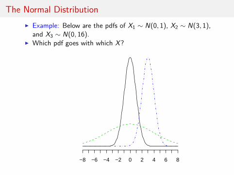
The Normal DistributionI Example: Below are the pdfs of X1 ∼ N(0, 1), X2 ∼ N(3, 1),

and X3 ∼ N(0, 16).I Which pdf goes with which X?

−8 −6 −4 −2 0 2 4 6 8

The Normal Distribution – Example

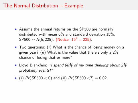
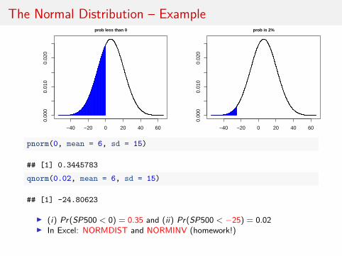
I Assume the annual returns on the SP500 are normallydistributed with mean 6% and standard deviation 15%.SP500 ∼ N(6, 225). (Notice: 152 = 225).

I Two questions: (i) What is the chance of losing money on agiven year? (ii) What is the value that there’s only a 2%chance of losing that or more?

I Lloyd Blankfein: “I spend 98% of my time thinking about 2%probability events!”

I (i) Pr(SP500 < 0) and (ii) Pr(SP500 <?) = 0.02

The Normal Distribution – Example

−40 −20 0 20 40 60

0.00

00.

010

0.02

0

sp500

prob less than 0

−40 −20 0 20 40 60

0.00

00.

010

0.02

0

sp500

prob is 2%

pnorm(0, mean = 6, sd = 15)

## [1] 0.3445783

qnorm(0.02, mean = 6, sd = 15)

## [1] -24.80623

I (i) Pr(SP500 < 0) = 0.35 and (ii) Pr(SP500 < −25) = 0.02I In Excel: NORMDIST and NORMINV (homework!)


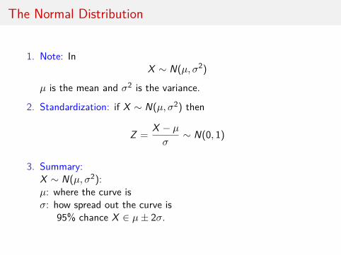
1. Note: InX ∼ N(µ, σ2)

µ is the mean and σ2 is the variance.

2. Standardization: if X ∼ N(µ, σ2) then

Z = X − µσ∼ N(0, 1)

3. Summary:X ∼ N(µ, σ2):µ: where the curve isσ: how spread out the curve is

95% chance X ∈ µ± 2σ.

The Normal Distribution – Another Example

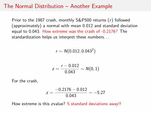
Prior to the 1987 crash, monthly S&P500 returns (r) followed(approximately) a normal with mean 0.012 and standard deviationequal to 0.043. How extreme was the crash of -0.2176? Thestandardization helps us interpret these numbers. . .

r ∼ N(0.012, 0.0432)

z = r − 0.0120.043 ∼ N(0, 1)

For the crash,

z = −0.2176− 0.0120.043 = −5.27

How extreme is this zvalue? 5 standard deviations away!!

The Normal Distribution – Approximating repeated trials

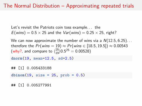
Let’s revisit the Patriots coin toss example. . . theE (wins) = 0.5× 25 and the Var(wins) = 0.25× 25, right?

We can now approximate the number of wins via a N(12.5, 6.25). . .therefore the Pr(wins = 19) ≈ Pr(wins ∈ [18.5, 19.5]) ≈ 0.00543(why?, and compare to

(2519)0.525 = 0.00528)

dnorm(19, mean=12.5, sd=2.5)

## [1] 0.005433188dbinom(19, size = 25, prob = 0.5)

## [1] 0.005277991

The Normal Distribution – Approximating repeated trials

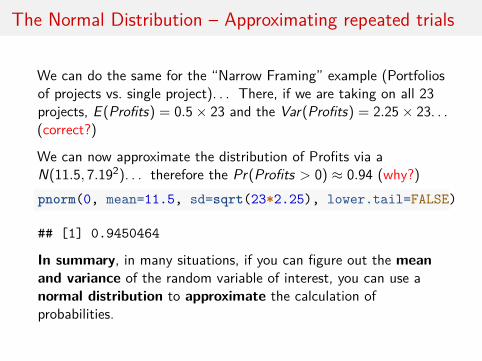
We can do the same for the “Narrow Framing” example (Portfoliosof projects vs. single project). . . There, if we are taking on all 23projects, E (Profits) = 0.5× 23 and the Var(Profits) = 2.25× 23. . .(correct?)

We can now approximate the distribution of Profits via aN(11.5, 7.192). . . therefore the Pr(Profits > 0) ≈ 0.94 (why?)pnorm(0, mean=11.5, sd=sqrt(23*2.25), lower.tail=FALSE)

## [1] 0.9450464

In summary, in many situations, if you can figure out the meanand variance of the random variable of interest, you can use anormal distribution to approximate the calculation ofprobabilities.

Portfolios, once again. . .

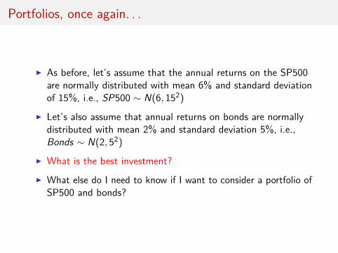
I As before, let’s assume that the annual returns on the SP500are normally distributed with mean 6% and standard deviationof 15%, i.e., SP500 ∼ N(6, 152)

I Let’s also assume that annual returns on bonds are normallydistributed with mean 2% and standard deviation 5%, i.e.,Bonds ∼ N(2, 52)

I What is the best investment?

I What else do I need to know if I want to consider a portfolio ofSP500 and bonds?

Portfolios once again. . .

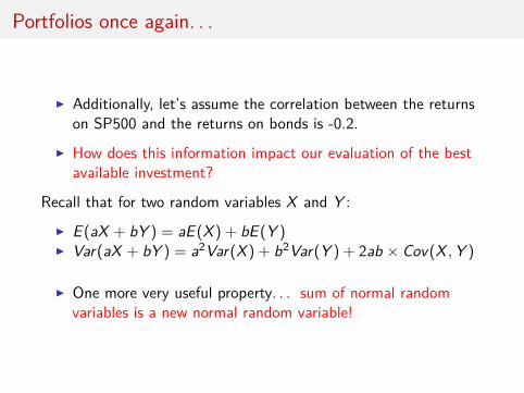
I Additionally, let’s assume the correlation between the returnson SP500 and the returns on bonds is -0.2.

I How does this information impact our evaluation of the bestavailable investment?

Recall that for two random variables X and Y :

I E (aX + bY ) = aE (X ) + bE (Y )I Var(aX + bY ) = a2Var(X ) + b2Var(Y ) + 2ab × Cov(X ,Y )

I One more very useful property. . . sum of normal randomvariables is a new normal random variable!

Portfolios once again. . .

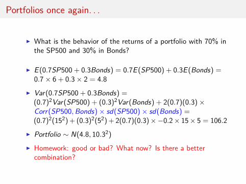
I What is the behavior of the returns of a portfolio with 70% inthe SP500 and 30% in Bonds?

I E (0.7SP500 + 0.3Bonds) = 0.7E (SP500) + 0.3E (Bonds) =0.7× 6 + 0.3× 2 = 4.8

I Var(0.7SP500 + 0.3Bonds) =(0.7)2Var(SP500) + (0.3)2Var(Bonds) + 2(0.7)(0.3)×Corr(SP500,Bonds)× sd(SP500)× sd(Bonds) =(0.7)2(152) + (0.3)2(52) + 2(0.7)(0.3)×−0.2× 15× 5 = 106.2

I Portfolio ∼ N(4.8, 10.32)

I Homework: good or bad? What now? Is there a bettercombination?

Median, Skewness

I The median of a random variable X is the point such thatthere is 50% chance X is above it, and hence a 50% chance Xis below it.

I For symmetric distributions, the expected value (mean) and themedian are always the same. . . look at all of our normaldistribution examples.

I But sometimes, distributions are skewed, i.e., not symmetric.In those cases the median becomes another helpful summary!

Median, Skewness

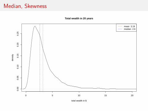
I Let’s think of an example. . . imagine you invest $1 in theSP500 today and want to know how much money you aregoing to have in 20 years. We can assume, once again, thatthe returns on the SP500 on a given year follow N(6, 152)

I Let’s also assume returns are independent year after year. . .

I Are my total returns just the sum of returns over 20 years?Not quite. . . compounding gets in the way.

Let’s simulate potential “futures”

Median, Skewness

0 5 10 15 20

0.00

0.05

0.10

0.15

0.20

0.25

Total wealth in 20 years

total wealth in $

dens

ity

mean 3.19median 2.6

Median, Skewness: R Code

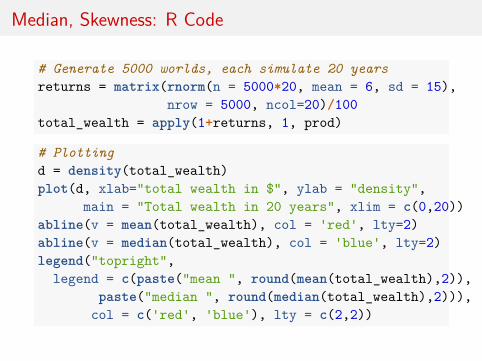
# Generate 5000 worlds, each simulate 20 yearsreturns = matrix(rnorm(n = 5000*20, mean = 6, sd = 15),

nrow = 5000, ncol=20)/100total_wealth = apply(1+returns, 1, prod)

# Plottingd = density(total_wealth)plot(d, xlab="total wealth in $", ylab = "density",

main = "Total wealth in 20 years", xlim = c(0,20))abline(v = mean(total_wealth), col = 'red', lty=2)abline(v = median(total_wealth), col = 'blue', lty=2)legend("topright",

legend = c(paste("mean ", round(mean(total_wealth),2)),paste("median ", round(median(total_wealth),2))),

col = c('red', 'blue'), lty = c(2,2))

The Berkeley gender bias case


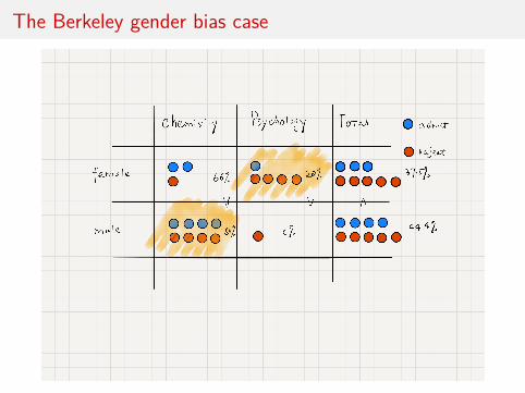
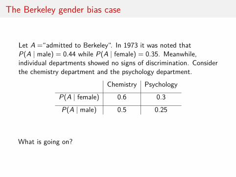
Let A =“admitted to Berkeley“. In 1973 it was noted thatP(A | male) = 0.44 while P(A | female) = 0.35. Meanwhile,individual departments showed no signs of discrimination. Considerthe chemistry department and the psychology department.

Chemistry Psychology

P(A | female) 0.6 0.3

P(A | male) 0.5 0.25

What is going on?


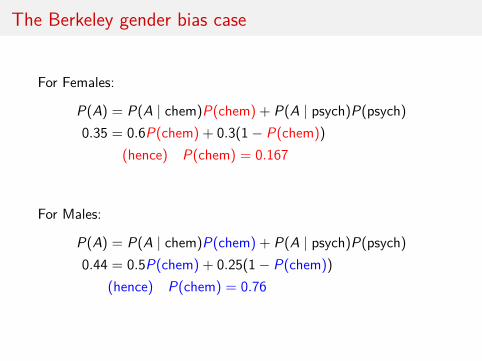
For Females:

P(A) = P(A | chem)P(chem) + P(A | psych)P(psych)0.35 = 0.6P(chem) + 0.3(1− P(chem))

(hence) P(chem) = 0.167

For Males:

P(A) = P(A | chem)P(chem) + P(A | psych)P(psych)0.44 = 0.5P(chem) + 0.25(1− P(chem))

(hence) P(chem) = 0.76


The explanation for the apparent overall bias was that women havea higher probability of applying to Psychology than to Chemistry(assuming for simplicity that these are the only two options) andoverall Psychology has a lower admissions rate!

This is a cautionary tale! Before we can act on a apparentassociation between two variables (for example, sue Berkeley) weneed to account for potential lurking variables that are the realcause of the relationship. We will talk a lot more about this. . . butkeep in mind, association is NOT causation!

Documents

Section1: Introduction,ProbabilityConcepts andDecisions · CourseOverview Section 1: Introduction,ProbabilityConceptsandDecisions Section 2: LearningfromData: Estimation,ConﬁdenceIntervals