TOMSK POLYTECHNIC UNIVERSITY

Timur R. Rakhimov

Financial Management

Textbook

Tomsk 2009

2

UDС

T. R. Rakhimov. Financial Management. Textbook. Tomsk: TPU Press, 2009, 75 pp.

This textbook consists of 3 sections devoted to the subject of Financial Management

The textbook is developed and prepared at the TPU Economic Engi-neering Department. It is recommended (intended) for foreign students following the Bachelor Degree Program in Management at Tomsk Poly-technic University.

Reviewed by: I.E. Nikulina, Head of Management Chair of Eco-nomic Engineering Department, TPU, C.E.Sc.

© Tomsk Polytechnic University, 2009

3

PREFACE

This Textbook is devoted to essential aspects of Financial Management on the micro level (company level). It is helpful in conveying lectures and training classes in Financial Management Course for students going through the Bachelor Degree Program in Management.

Financial Management is a part of Management that deals with Fin-ances of a company. This textbook is designed as a study book and in-cludes sections that cover the following topics

- Financial Statements Evaluation,

- Financial Planning and Forecasting

- Capital Budgeting Analysis.

Here you may find answers to questions concerning financial ratios, their essence and ways of calculation; stages of financial planning; types of budgets in the company; basis for capital investment decision etc.

There is a Workbook that supplements the Textbook. The Workbook presents a set of financial problems for each section of the Textbook and is focused on obtaining practical experience and developing skills in solving of problems concerning regarded aspects of financial manage-ment.

The Workbook contains assignments, which the student must fulfil. The material in Work book is presented in accordance with sections and chapters of the Textbook.

The author welcomes yours suggestions for improvements of future edi-tions of this textbook.

4

Contents

PREFACE ...................................................................................................... 3

Contents ......................................................................................................... 4

Section I: Evaluating Financial Performance ............................................ 5

Chapter 1: Return on Equity ..................................................................... 5

Chapter 2: Liquidity Ratios ....................................................................... 7

Chapter 3: Asset Management Ratios ..................................................... 10

Chapter 4: Profitability Ratios ................................................................ 12

Chapter 5: Leverage Ratios ..................................................................... 13

Chapter 6: Market Value Ratios ............................................................. 15

Chapter 7: Comparing Financial Statements ......................................... 17

Chapter 8: Summary ................................................................................ 18

Terminology Section I: Evaluating Financial Performance ................. 20

Questions Section I: Evaluating Financial Performance...................... 24

True or False Section I: Evaluating Financial Performance ............... 25

Section II: Financial Planning and Forecasting ....................................... 26

Chapter 1: The First Steps ....................................................................... 26

Chapter 2: Detail Budgets ....................................................................... 28

Chapter 3: Budgeted Financial Statements ............................................ 31

Chapter 4: Additional Concepts in Budgeting ........................................ 38

Chapter 5: Making the Budgeting Process Work ................................... 42

Chapter 6: Summary ................................................................................ 45

Terminology Section II: Financial Planning and Forecasting ............. 46

Questions Section II: Evaluating Financial Performance .................... 50

True or False Section II: Financial Planning and Forecasting ........... 51

Section III: Capital Budgeting Analysis ................................................... 52

Chapter 1: The Overall Process .............................................................. 52

Chapter 2: Calculating the Discounted Cash Flows of Projects ........... 58

Chapter 3: Three Economic Criteria for Evaluating Capital Projects.. 62

Chapter 4: Additional Considerations in Capital Budgeting Analysis .. 66

Chapter 5: Course Summary ................................................................... 67

Terminology Section III: Capital Budgeting Analysis ........................... 69

Questions Section III: Capital Budgeting Analysis ............................... 72

True or False Section III: Capital Budgeting Analysis ......................... 73

Sources and References .............................................................................. 74

5

Section I: Evaluating Financial Perfor-

mance

Chapter 1: Return on Equity

Ratios

It is said that you must measure what you expect to manage and ac-complish. Without measurement, you have no reference to work with and thus, you tend to operate in the dark. One way of establishing refer-ences and managing the financial affairs of an organization is to use ra-tios. Ratios are simply relationships between two financial balances or financial calculations. These relationships establish our references so we can understand how well we are performing financially. Ratios also extend our traditional way of measuring financial performance; i.e. rely-ing on financial statements. By applying ratios to a set of financial statements, we can better understand financial performance.

Calculating Return on Equity

For publicly traded companies, the relationship of earnings to equity or Return on Equity is of prime importance since management must pro-vide a return for the money invested by shareholders. Return on Equity is a measure of how well management has used the capital invested by shareholders. Return on Equity tells us the percent returned for each dollar (or other monetary unit) invested by shareholders. Return on Eq-uity is calculated by dividing Net Income by Average Shareholders Equi-ty (including Retained Earnings).

EXAMPLE — Net Income for the year was $60,000, total sharehold-er equity at the beginning of the year was $315,000 and ending shareholder equity for the year was $285,000. Return on Equity is calculated by dividing $60,000 by $300,000 (average shareholders equity which is ($315,000 + $285,000) / 2). This gives us a Return on Equity of 20%. For each dollar invested by shareholders, 20% was returned in the form of earnings.

SUMMARY — Return on Equity is one of the most widely used ra-tios for publicly traded companies. It measures how much return

6

management was able to generate for the shareholders. The formula for calculating Return on Equity is:

Net Income / Average Shareholders Equity

Components of Return on Equity

Return on Equity has three ratio components. The three ratios that make up Return on Equity are:

1. Profit Margin = Net Income / Sales

2. Asset Turnover = Sales / Assets

3. Financial Leverage = Assets / Equity

Profit Margin measures the percent of profits you generate for each dol-lar of sales. Profit Margin reflects your ability to control costs and make a return on your sales. Profit Margin is calculated by dividing Net Income by Sales. Management is interested in having high profit margins.

EXAMPLE — Net Income for the year was $60,000 and Sales were $480,000. Profit Margin is $60,000 / $480,000 or 12.5%. For each dollar of sales, we generated $0.125 of profits.

Asset Turnover measures the percent of sales you are able to generate from your assets. Asset Turnover reflects the level of capital we have tied-up in assets and how much sales we can squeeze out of our as-sets. Asset Turnover is calculated by dividing Sales by Average Assets. A high asset turnover rate implies that we can generate strong sales from a relatively low level of capital. Low turnover would imply a very capital-intensive organization.

EXAMPLE — Sales for the year were $480,000, beginning total as-sets were $505,000 and year-end total assets are $495,000. The Asset Turnover Rate is $480,000 / $500,000 (average total assets which is ($505,000 + $495,000) / 2) or 0.96. For every $1.00 of as-sets, we were able to generate $0.96 of sales.

Financial Leverage is the third and final component of Return on Equity. Financial Leverage is a measure of how much we use equity and debt

7

to finance our assets. As debt increases, The financial leverage in-creases. Generally, management tends to prefer equity financing over debt since it carries less risk. The Financial Leverage Ratio is calculated by dividing Assets by Shareholder Equity.

EXAMPLE — Average assets are $500,000 and average share-holder equity is $320,000. Financial Leverage Ratio is $500,000 / $20,000 or 1.56. For each $1.56 in assets, we are using $1.00 in eq-uity financing.

Now let us compare our Return on Equity to a combination of three component ratios:

From our example, Return on Equity = $60,000 / $320,000 or 18.75% or we can combine the three components of Return on Equity from our examples:

Profit Margin x Asset Turnover x Financial Leverage = Return on Equity or 0.125 x 0.96 x 1.56 = 18.75%.

Now that we understand the basic ratio structure, we can move down to a more detail analysis with ratios. Four common groups of detail ratios are: Liquidity, Asset Management, Profitability and Leverage. We will al-so look at market value ratios.

Chapter 2: Liquidity Ratios

Liquidity Ratios help us understand if we can meet our obligations over the short-run. Higher liquidity levels indicate that we can easily meet our current obligations. We can use several types of ratios to monitor liquidi-ty.

Current Ratio

Current Ratio is simply current assets divided by current liabilities. Cur-rent assets include cash, accounts receivable, marketable securities, in-ventories, and prepaid items. Current liabilities include accounts paya-ble, notes payable, salaries payable, taxes payable, current maturities of long-term obligations and other current accruals.

C urrent AssetsC urrent Liquidity R atio =

C urrent Liabilities

8

C AC LR

C L

EXAMPLE — Current Assets are $200,000 and Current Liabilities are $80,000. The Current Ratio is $200,000 / $80,000 or 2.5. We have 2.5 times more current assets than current liabilities.

A low current ratio would imply possible insolvency problems. A very high current ratio might imply that management is not investing idle as-sets productively. Generally, we want to have a current ratio that is pro-portional to our operating cycle. We will look at the Operating Cycle as part of asset management ratios.

Acid Test (Quick Ratio)

Since certain current assets (such as inventories) may be difficult to convert into cash, we may want to modify the Current Ratio. Also, if we use the LIFO (Last In First Out) Method for inventory accounting, our current ratio will be understated. Therefore, we will remove certain cur-rent assets from our previous calculation. This new ratio is called the Ac-id Test or Quick Ratio; i.e. assets that are quickly converted into cash will be compared to current liabilities. The Acid Test Ratio measures our ability to meet current obligations based on the liquid assets. Liquid as-sets include cash, marketable securities, and accounts receivable. The Acid Test Ratio is calculated by dividing the sum of our liquid assets by current liabilities.

C ash + M arketable Securities + Accounts PayableQ uick R atio =

C urrent Liabilities

C M S ARQ R

C L

EXAMPLE — Cash is $5,000, Marketable Securities are $15,000, Accounts Receivable are $40,000, and Current Liabilities are $80,000. The Acid Test Ratio is ($5,000 + $15,000 + $40,000) / $80,000 or 0.75. We have $0.75 in liquid assets for each $1.00 in current liabilities.

9

Cash Ratio

Sometimes it may be necessary to measure our ability to meet current obligations based on the most liquid assets, which include only cash and marketable securities. Therefore Cash Ratio will be calculated by dividing the sum of most liquid assets by current liabilities

C ash + M arketable SecuritiesC ash R atio =

C urrent Liabilities

C M SC R

C L

EXAMPLE — The Cash Ratio from a previous example is ($5,000 + $15,000) / $80,000 or 0.25. We have $0.25 in most liquid assets for each $1.00 in current liabilities.

It is desirable, that this ratio is more than 0.2

Defensive Interval

Defensive Interval is the sum of liquid assets compared to our expected daily cash outflows. The Defensive Interval is calculated as follows:

(Cash + Marketable Securities + Receivables) / Daily Operating Cash Outflow

EXAMPLE — Referring back to our last example, we have total quick assets of $60,000 and we have estimated that our daily operat-ing cash outflow is $1,200. This would give us a 50 day defensive in-terval ($60,000 / $1,200). We have 50 days of liquid assets to cover our cash outflows.

Ratio of Operating Cash Flow to Current Debt Obligations

The Ratio of Operating Cash Flow to Current Debt Obligations places emphasis on cash flows to meet fixed debt obligations. Current maturi-ties of long-term debts along with notes payable comprise our current debt obligations. We can refer to the Statement of Cash Flows for oper-ating cash flows. Therefore, the Ratio of Operating Cash Flow to Cur-rent Debt Obligations is calculated as follows:

Operating Cash Flow / (Current Maturity of Long-Term Debt + Notes Payable)

10

EXAMPLE — We have operating cash flow of $100,000, notes pay-able of $20,000 and we have $5,000 in current obligations related to our long-term debt. The Operating Cash Flow to Current Debt Obli-gations Ratio is $100,000 / ($20,000 + $5,000) or 4.0. We have 4 times the cash flow to cover our current debt obligations.

Chapter 3: Asset Management Ratios

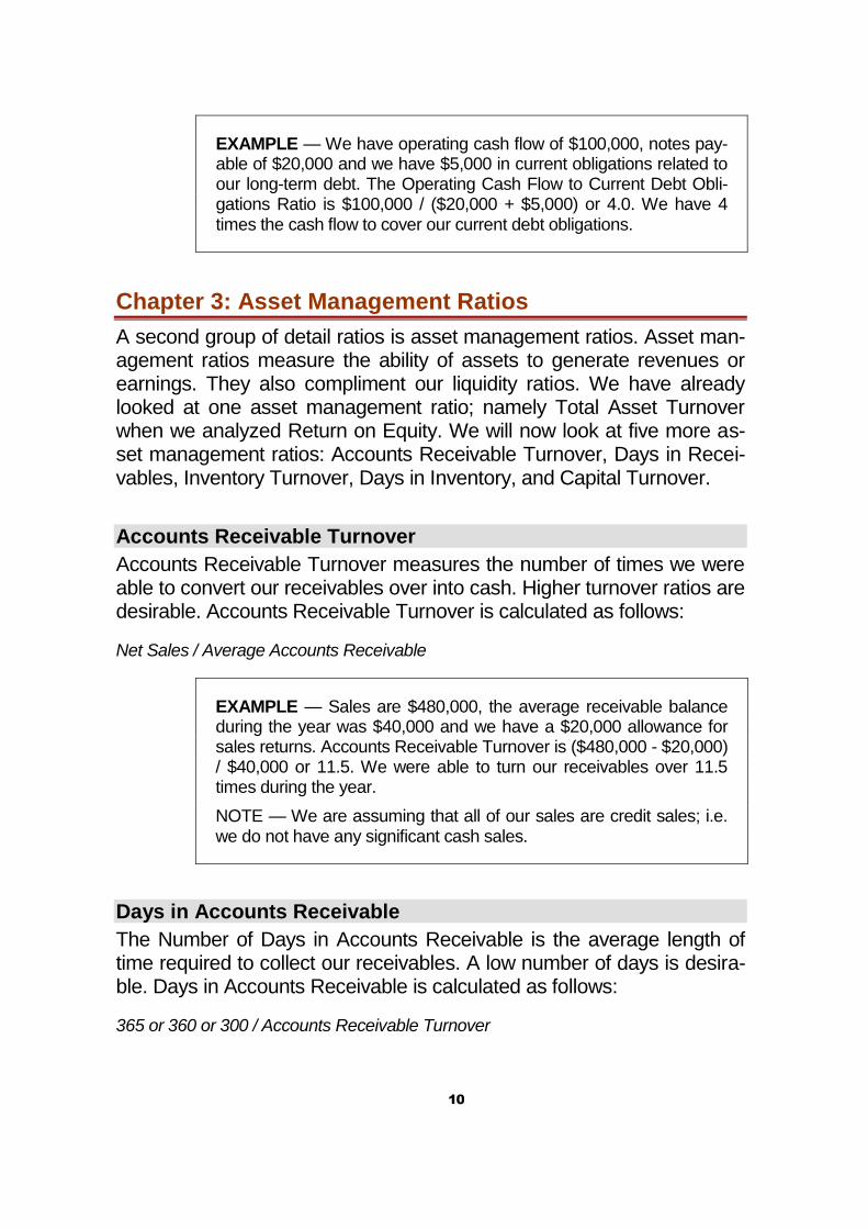
A second group of detail ratios is asset management ratios. Asset man-agement ratios measure the ability of assets to generate revenues or earnings. They also compliment our liquidity ratios. We have already looked at one asset management ratio; namely Total Asset Turnover when we analyzed Return on Equity. We will now look at five more as-set management ratios: Accounts Receivable Turnover, Days in Recei-vables, Inventory Turnover, Days in Inventory, and Capital Turnover.

Accounts Receivable Turnover

Accounts Receivable Turnover measures the number of times we were able to convert our receivables over into cash. Higher turnover ratios are desirable. Accounts Receivable Turnover is calculated as follows:

Net Sales / Average Accounts Receivable

EXAMPLE — Sales are $480,000, the average receivable balance during the year was $40,000 and we have a $20,000 allowance for sales returns. Accounts Receivable Turnover is ($480,000 - $20,000) / $40,000 or 11.5. We were able to turn our receivables over 11.5 times during the year.

NOTE — We are assuming that all of our sales are credit sales; i.e. we do not have any significant cash sales.

Days in Accounts Receivable

The Number of Days in Accounts Receivable is the average length of time required to collect our receivables. A low number of days is desira-ble. Days in Accounts Receivable is calculated as follows:

365 or 360 or 300 / Accounts Receivable Turnover

11

EXAMPLE — If we refer to our previous example and we base our calculation on the full calendar year, we would require 32 days on average to collect our receivables. 365 / 11.5 = 32 days.

Inventory Turnover

Inventory Turnover is similar to accounts receivable turnover. We are measuring how many times did we turn our inventory over during the year. Higher turnover rates are desirable. A high turnover rate implies that management does not hold onto excess inventories and our inven-tories are highly marketable. Inventory Turnover is calculated as follows:

Cost of Sales / Average Inventory

EXAMPLE — Cost of Sales were $192,000 and the average inven-tory balance during the year was $120,000. The Inventory Turnover Rate is 1.6 or we were able to turn our inventory over 1.6 times dur-ing the year.

Days in Inventory

Days in Inventory is the average number of days we held our inventory before a sale. A low number of inventory days is desirable. A high num-ber of days implies that management is unable to sell existing inventory stocks. Days in Inventory is calculated as follows:

365 or 360 or 300 / Inventory Turnover

EXAMPLE — If we refer back to the previous example and we use the entire calendar year for measuring inventory, then on average we are holding our inventories 228 days before a sale. 365 / 1.6 = 228 days.

Operating Cycle

Now that we have calculated the number of days for receivables and the number of days for inventory, we can estimate our operating cycle. Op-erating Cycle = Number of Days in Receivables + Number of Days in Inventory. In our previous examples, this would be 32 + 228 = 260 days.

12

So on average, it takes us 260 days to generate cash from our current assets.

If we look back at our Current Ratio, we found that we had 2.5 times more current assets than current liabilities. We now want to compare our Current Ratio to our Operating Cycle. Our turnover within the Oper-ating Cycle is 365 / 260 or 1.40. This is lower than our Current Ratio of 2.5. This indicates that we have additional assets to cover the turnover of current assets into cash. If our current ratio were below that of the Operating Cycle Turnover Rate, this would imply that we do not have sufficient current assets to cover current liabilities within the Operating Cycle. We may have to borrow short-term debt to pay our expenses.

Capital Turnover

One final turnover ratio that we can calculate is Capital Turnover. Capi-tal Turnover measures our ability to turn capital over into sales. Re-member, we have two sources of capital: Debt and Equity. Capital Turnover is calculated as follows:

Net Sales / Interest Bearing Debt + Shareholders Equity

EXAMPLE — Net Sales are $460,000, we have $50,000 in Debt and $200,000 of Equity. Capital Turnover is $460,000 / ($50,000 + $200,000) = 1.84. For each $1.00 of capital invested (both debt and equity), we are able to generate $1.84 in sales.

Chapter 4: Profitability Ratios

A third group of ratios that we can use are profitability ratios. Profitability Ratios measure the level of earnings in comparison to a base, such as assets, sales, or capital. We have already reviewed two profitability ra-tios: Return on Equity and Profit Margin. Two other ratios we can use to measure profitability are Operating Income to Sales and Return on As-sets.

Operating Income to Sales

Operating Income to Sales compares Earnings Before Interest and Taxes (EBIT) to Sales. By using EBIT, we place more emphasis on op-

13

erating results and follow cash flow concepts more closely. Operating Income to Sales is calculated as follows:

EBIT / Net Sales

EXAMPLE — Net Sales are $460,000 and Earnings Before Interest and Taxes is $100,000. This gives us a return of 22% on sales, $100,000 / $460,000 = 0.22. For every $1.00 of sales, we generated $0.22 in Operating Income.

Return on Assets

Return on Assets measures the net income returned on each dollar of assets. This ratio measures overall profitability from our investment in assets. Higher rates of return are desirable. Return on Assets is calcu-lated as follows:

Net Income / Average Total Assets

EXAMPLE — Net Income is $60,000 and average total assets for the year are $500,000. This gives us a 12% return on assets, $60,000 / $500.000 = 0.12.

Return on Assets is often modified to ensure accurate measurement of returns. For example, we may want to deduct out preferred dividends from Net Income or maybe we should include operating assets only and exclude intangibles, investments, and other assets not managed for an overall rate of return.

Chapter 5: Leverage Ratios

Another important group of detail ratios are Leverage Ratios. Leverage Ratios measure the use of debt and equity for financing of assets. We previously looked at the Financial Leverage Ratio as part of Return on Equity. Three other leverage ratios that we can use are Debt to Equity, Debt Ratio, and Times Interest Earned.

Debt to Equity

Debt to Equity is the ratio of Total Debt to Total Equity. It compares the funds provided by creditors to the funds provided by shareholders. As

14

more debt is used, the Debt to Equity Ratio will increase. Since we incur more fixed interest obligations with debt, risk increases. On the other hand, the use of debt can help improve earnings since we get to deduct interest expense on the tax return. So we want to balance the use of debt and equity such that we maximize our profits, but at the same time manage our risk. The Debt to Equity Ratio is calculated as follows:

Total Liabilities / Shareholders Equity

EXAMPLE — We have total liabilities of $75,000 and total share-holders equity of $200,000. The Debt to Equity Ratio is 37.5%, $75,000 / $200,000 = 0.375. When compared to our equity re-sources, 37.5% of our resources are in the form of debt.

KEY POINT — As a general rule, it is advantageous to increase our use of debt (trading on the equity) if earnings from borrowed funds exceeds the costs of borrowing.

Debt Ratio

The Debt Ratio measures the level of debt in relation to our investment in assets. The Debt Ratio tells us the percent of funds provided by credi-tors and to what extent our assets protect us from creditors. A low Debt Ratio would indicate that we have sufficient assets to cover our debt load. Creditors and management favor a low Debt Ratio. The Debt Ratio is calculated as follows:

Total Liabilities / Total Assets

EXAMPLE — Total Liabilities are $75,000 and Total Assets are $500,000. The Debt Ratio is 15%, $75,000 / $500,000 = 0.15. 15% of our funds for assets comes from debt.

NOTE — We use Total Liabilities to be conservative in our assess-ment.

Times Interest Earned

Times Interest Earned is the number of times our earnings (before inter-est and taxes) covers our interest expense. It represents our margin of safety in making fixed interest payments. A high ratio is desirable from

15

both creditors and management. Times Interest Earned is calculated as follows:

Earnings Before Interest and Taxes / Interest Expense

EXAMPLE — Earnings Before Interest Taxes is $100,000 and we have $10,000 in Interest Expense. Times Interest Earned is 10 times, $100,000 / $10,000. We are able to cover our interest ex-penses 10 times with operating income.

Chapter 6: Market Value Ratios

One final group of detail ratios that warrants some attention is Market Value Ratios. These ratios attempt to measure the economic status of the organization within the marketplace. Investors use these ratios to evaluate and monitor the progress of their investments.

Earnings Per Share

Growth in earnings is often monitored with Earnings per Share (EPS). The EPS expresses the earnings of a company on a "per share" basis. A high EPS in comparison to other competing firms is desirable. The EPS is calculated as:

Earnings Available to Common Shareholders / Number of Common Shares Out-standing

EXAMPLE — Earnings are $100,000 and preferred stock dividends of $20,000 need to be paid. There are a total of 80,000 common shares outstanding. Earnings per Share (EPS) is ($100,000 - $20,000) / 80,000 shares outstanding or $1.00 per share.

P/E Ratio

The relationship of the price of the stock in relation to EPS is expressed as the Price to Earnings Ratio or P/E Ratio. Investors often refer to the P/E Ratio as a rough indicator of value for a company. A high P/E Ratio would imply that investors are very optimistic (bullish) about the future of the company since the price (which reflects market value) is selling for well above current earnings. A low P/E Ratio would imply that investors view the company's future as poor and thus, the price the company sells

16

for is relatively low when compared to its earnings. The P/E Ratio is cal-culated as follows:

Price of Stock / Earnings per Share *

* Earnings per Share are fully diluted to reflect the conversion of securities into com-mon stock.

EXAMPLE — Earnings per share is $3.00 and the stock is selling for $36.00 per share. The P/E Ratio is $36 / $3 or 12. The company is selling for 12 times earnings.

Book Value per Share

Book Value per Share expresses the total net assets of a business on a per share basis. This allows us to compare the book values of a busi-ness to the stock price and gauge differences in valuations. Net Assets available to shareholders can be calculated as Total Equity less Pre-ferred Equity. Book Value per Share is calculated as follows:

Net Assets Available to Common Shareholders * / Outstanding Common Shares

* Calculated as Total Equity less Preferred Equity.

EXAMPLE — Total Equity is $5,000,000 including $400,000 of pre-ferred equity. The total number of common shares outstanding is 80,000 shares. Book Value per Share is ($5,000,000 - $400,000) / 80,000 or $57.50

Dividend Yield

The percentage of dividends paid to shareholders in relation to the price of the stock is called the Dividend Yield. For investors interested in a source of income, the dividend yield is important since it gives the inves-tor an indication of how much dividends are paid by the company. Divi-dend Yield is calculated as follows:

Dividends per Share / Price of Stock

17

EXAMPLE — Dividends per share are $2.10 and the price of the stock is $30.00 per share. The Dividend Yield is $2.10 / $30.00 or 7%

Chapter 7: Comparing Financial Statements

One final way of evaluating financial performance is simply to compare financial statements from period to period and to compare financial statements with other companies. This can be facilitated by vertical and horizontal analysis.

Vertical Analysis

Vertical analysis compares line items on a financial statement over an extended period of time. This helps us spot trends and restate financial statements to a common size for quick analysis. For the Balance Sheet, we will use total assets as our base (100%) and for the Income State-ment, we will use Sales as our base (100%). We will compare different line items on the financial statements to these bases and express the line items as a percentage of the base.

EXAMPLE — Income Statements for the last three years are sum-marized below: 1990 1991 1992 Sales $300,000 $310,000 $330,000 Cost of Goods Sold (110,000) (105,000) (110,000) G & A Expenses ( 80,000) (100,000) (105,000) Net Income $110,000 $105,000 $115,000 < - - - - - - - Vertical Analysis - - - - - - - - - > Sales 100% 100% 100% Cost of Goods Sold 37% 34% 33% G & A Expenses 27% 32% 32% Net Income 37% 34% 35% By expressing balances as percentages, we can easily notice that G

& A Expenses are trending up while Cost of Goods Sold is moving down. This may require further analysis to determine what is behind these trends.

18

Horizontal Analysis

Horizontal analysis looks at the percentage change in a line item from one period to the next. This helps us identify trends from the financial statements. Once we spot a trend, we can dig deeper and investigate why the change has occurred. The percentage change is calculated as:

(Dollar Amount in Year 2 - Dollar Amount in Year 1) / Dollar Amount in Year 1

EXAMPLE — Sales were $310,000 in 1991 and $330,000 in 1992. The percentage change in sales is:

($330,000 - $310,000) / $310,000 = 6.5%

We can apply this analysis "horizontally" down the financial state-ment for the year 1992:

Sales 6.5% Cost of Goods Sold 4.8% G & A Expenses 5.0% Net Income 9.5%

Chapter 8: Summary

We started our look at ratio analysis with Return on Equity since this one ratio is at the heart of financial management; namely we want to maxim-ize returns for the shareholders of the company. Secondly, we have three ways of influencing Return on Equity. We can change our profit margins, we can change our turnover of assets, or we can change our use of financial leverage. Next, we looked at how we can influence the three components of Return on Equity.

There are several detail ratios that we can monitor, such as acid test, inventory turnover, and debt to equity. Detail ratios help us monitor spe-cific financial conditions, such as liquidity or profitability.

Ratios are best used when compared or benchmarked against another reference, such as an industry standard or "best in class" within our in-dustry. This type of comparison helps us establish financial goals and identify problem areas.

19

We can also use vertical and horizontal analysis for easy identification of changes within financial balances.

It should be noted that ratios do have limitations. After all, ratios are usually derived from financial statements and financial statements have serious limitations. Additionally, comparisons are usually difficult be-cause of operating and financial differences between companies. None-the-less, if you want to analyze a set of financial statements, ratio analy-sis is probably one of the most popular approaches to understanding fi-nancial performance.

20

Terminology Section I: Evaluating Financial Performance

Chapter 1

Financial ratios ............................ = финансовые коэффициенты Financial balances ....................... = финансовые сальдо Financial statement ..................... = финансовая отчетность Earnings ...................................... = доход, прибыль, поступления. Equity ........................................... = собственный (акционерный)

капитал Return .......................................... = прибыль, доход, выручка Net Income .................................. = Чистый доход Average Shareholders Equity ...... = Средний Акционерный

Капитал Retained Earnings ....................... = Нераспределенная прибыль Profit margin ................................ = Уровень прибыли или Рента-

бельность Sales ............................................ = Объем продаж Asset turnover .............................. = Оборачиваемость всех акти-

вов Financial Leverage ....................... = Финансовый левередж или по-

казатель использования заем-ных средств

Chapter 2

Liquidity Ratios ............................ = Коэффициенты ликвидности Current Liquidity Ratio ................. = Коэффициент текущей

ликвидности Current Assets ............................. = оборотные фонды, оборотные

средства (денежные средства, вложенные в запасы сырья, материалов, топлива, готовой продукции, а также счета в банках)

Current Liabilities ......................... = Краткосрочные обязательства Cash ............................................ = наличные денежные средства

(средства в кассе) Accounts Receivable ................... = дебиторская задолженность

21

Marketable securities ................... = легко реализуемые ценные бумаги

Inventories ................................... = наличные товары, материально производствен-ные запасы

Prepaid items ............................... = авансируемые средства (предоплаченные средства)

Accounts payable ......................... = кредиторская задолженность (счета к оплате)

Notes payable .............................. = Векселя к оплате = bill, bill of credit, paper, loan note

Salaries Payable .......................... = Задолженность по оплате тру-да

Taxes Payable ............................. = Налоги подлежащие к уплате в бюджет

Maturity ........................................ = Срок платежа по векселю Current Accruals .......................... = Текущие начисления Insolvency problems .................... = банкротство, несостоятель-

ность Acid Test Ratio (Quick Ratio) ....... = Коэффициент критической

оценки (отношение ликвидно-сти фирмы к сумме долговых обязательств) = коэффициент быстрой ликвидности.

i.e. ............................................... = (id est; лат) = that is = то есть e.g. ............................................... = (exemli gratia; лат) = for exam-

ple = например Operating Cash Flow ................... = текущий поток наличности

(денежных средств) Current Debt Obligations .............. = текущие долговые обязатель-

ства Cash Flow Statement ................... = отчет об оборотных средствах

(баланс оборотных средств)

Chapter 3

Asset Management Ratios ........... = Коэффициенты управления активами

Accounts Receivable Turnover .... = Оборачиваемость дебитор-ской задолженности

Sales Return ................................ = доход от продаж Sales Returns .............................. = возвращенный товар

22

Allowance for Sales Returns ........ = норма возвращенного товара (поправка на возвращенный товар)

Days in Accounts Receivable ....... = Период оборота дебиторской задолженности

Inventory Turnover ....................... = Оборачиваемость материаль-ных запасов

Excess Inventories ....................... = излишние запасы Cost of Sales ............................... = Себестоимость реализован-

ной продукции Days in Inventory ......................... = Период оборота материаль-

ных запасов Inventory Stocks .......................... = Запасы товаров на складе Operating Cycle ........................... = Операционный цикл Receivables ................................. = Дебиторы Debtor .......................................... = Дебитор Debtee ......................................... = Creditor, Lender, Tenderer =

Кредитор Capital Turnover .......................... = Оборачиваемость капитала

Chapter 4

Profitability Ratios ........................ = Коэффициенты рентабельно-сти (доходности)

Operating Income ........................ = Операционная прибыль (до-ход)

EBIT (Earnings Before Interest and Taxes) = Прибыль до уп-латы процентов и налогов (Балансовая прибыль)

Return on Assets ......................... = Рентабельность активов

Chapter 5

Leverage Ratios ........................... = Коэффициенты левереджа Interest Earned ............................ = Полученные проценты Times Interest Earned .................. = Отношение балансовой при-

были к процентным издержкам (Балансовая рентабельность процентных издержек)

Chapter 6

Market Value Ratios ..................... = Коэффициенты рыночной стоимости

23

EPS ............................................. = Earnings per Share Preferred stock Dividends ............ = Дивиденды по

привилегированным акциям Common Shares Outstanding ...... = Обыкновенные акции, выпу-

щенные в оборот P/E Ratio...................................... = Price to Earnings Ratio Bullish .......................................... = Играющий на повышение

(Bearish = играющий на пони-жение, снижающийся) о рынке ценных бумаг

Book Value .................................. = нетто-капитал, остаточная стоимость капитала

Book Value per Share .................. = доля нетто-капитала на одну акцию

face / nominal value ..................... = номинальная стоимость depreciated value ......................... = остаточная стоимость replacement value ........................ = восстановительная стоимость balance sheet value ..................... = балансовая стоимость salvage value ............................... = ликвидационная стоимость Dividend Yield .............................. = доходность акций (дивиденды

/ стоимость акций) G & A Expenses........................... = (General & Administrative Ex-

penses) Общие и административные расходы

24

Questions Section I: Evaluating Financial Performance

NOTE: The following questions are based on the material of the section and imply answers in a form of discussion

1. How would you explain what a financial ratio is?

2. What is the benefit of using financial ratios in financial manage-ment?

3. What does Return on Equity Ratio show?

4. How do you understand Liquidity of a company?

5. What is included in current assets?

6. What is included in current liabilities?

7. What does defensive interval show?

8. What does Operating Cycle show?

9. What does Capital Turnover show?

10. How do you understand Leverage?

25

True or False Section I: Evaluating Financial Performance

Mark the following statements True if you agree with it or False if you don’t agree with the statement?

1. Ratio is a relationship between two financial balances or finan-cial calculations. _________

2. Return on Equity tells the percent returned on each dollar in-vested in total assets _________

3. High liquidity levels show that we can easily meet our obliga-tions. _________

4. Acid test and Current Ratio mean the same thing. _________ 5. Liquidity Ratios help us understand whether a company may

face insolvency problems. _________ 6. Accounts receivable show what creditors are supposed to re-

ceive from the company. _________ 7. Accounts payable show what the company has to pay to its

creditors _________ 8. The higher inventory turnover rate is the better. _________ 9. Capital turnover measures our ability to turn sales over into capi-

tal. _________ 10. Leverage Ratios measure the use of equity and debt for financ-

ing assets. _________ 11. Earnings per share is calculated as follows: Earnings divided by

Number of Common shares outstanding. _________ 12. High P/E ratio indicates that investors are bullish (optimistic)

about the future of a company. _________ 13. Dividend yield for preferred shareholders is usually fixed and

doesn’t depend on the profit that the company earns._________ 14. Vertical analysis compares line item dynamics on a financial

statement over an extended period of time. _________

26

Section II: Financial Planning and Fore-

casting

Chapter 1: The First Steps

Introduction

Financial planning is a continuous process of directing and allocating fi-nancial resources to meet strategic goals and objectives. The output from financial planning takes the form of budgets. The most widely used form of budgets is Pro Forma or Budgeted Financial Statements. The foundation for Budgeted Financial Statements is Detail Budgets. Detail Budgets include sales forecasts, production forecasts, and other esti-mates in support of the Financial Plan. Collectively, all of these budgets are referred to as the Master Budget.

We can also break financial planning down into planning for operations and planning for financing. Operating people focus on sales and produc-tion while financial planners are interested in how to finance the opera-tions. Therefore, we can have an Operating Plan and a Financial Plan. However, to keep things simple and to make sure we integrate the process fully, we will consider financial planning as one single process that encompasses both operations and financing.

Start with Strategic Planning

Financial Planning starts at the top of the organization with strategic planning. Since strategic decisions have financial implications, you must start your budgeting process within the strategic planning process. Fail-ure to link and connect budgeting with strategic planning can result in budgets that are "dead on arrival."

Strategic planning is a formal process for establishing goals and objec-tives over the long run. Strategic planning involves developing a mission statement that captures why the organization exists and plans for how the organization will thrive in the future. Strategic objectives and corres-ponding goals are developed based on a very thorough assessment of the organization and the external environment. Finally, strategic plans are implemented by developing an Operating or Action Plan. Within this

27

Operating Plan, we will include a complete set of financial plans or budgets.

Financial Plans (Budgets) Operating Plan Strategic Plan

The Sales Forecast

In order to develop budgets, we will start with a forecast of what drives much of our financial activity; namely sales. Therefore, the first forecast we will prepare is the Sales Forecast. In order to estimate sales, we will look at past sales histories and various factors that influence sales. For example, marketing research may reveal that future sales are expected to stabilize. Maybe we cannot meet growing sales because of limited production capacities or maybe there will be a general economic slow down resulting in falling sales. Therefore, we need to look at several fac-tors in arriving at our sales forecast.

After we have collected and analyzed all of the relevant information, we can estimate sales volumes for the planning period. It is very important that we arrive at a good estimate since this estimate will be used for several other estimates in our budgets. The Sales Forecast has to take into account what we expect to sell and at what sales price.

EXHIBIT 1 — SALES FORECAST Product Volume Price Total Sales Lace Shoes 16,000 $45.00 $720,000

Percent of Sales

Now we need to estimate account changes because of estimated sales. One way to estimate and forecast certain account balances is by means of the Percent of Sales Method. By looking at past account balances and past changes in sales, we can establish a percentage relationship. For example, all variable costs and most current assets and current lia-bilities will vary as sales change.

EXAMPLE 1 — ESTIMATED ACCOUNTS RECEIVABLE

Past history shows that accounts receivable runs around 30% of sales. We have estimated that next year's sales will be $160,000.

28

Therefore, our estimated accounts receivable is $48,000 ($160,000 x 0.30).

Chapter 2: Detail Budgets

We also need to prepare several detail budgets for developing a Bud-geted Income Statement. For example, production must be planned for our estimated sales of 16,000 units from Exhibit 1. The Production De-partment will need to budget for materials, labor, and overhead based on what we expect to sell and what we expect in inventory.

EXHIBIT 2 — PRODUCTION BUDGET Planned Sales (Exhibit 1) ........................................... 16,000 Desired Ending Inventory ........................................... 1,500 Total Units ................................................................... 17,500 Less Beginning Inventory .......................................... ( 3,000) Planned Production ................................................. 14,500

Once we have established our level of production (Exhibit 2), we can prepare a Materials Budget. The Materials Budget attempts to forecast the level of purchases required, taking into account materials required for production and inventory levels. We can summarize the materials to be purchased as:

Materials Purchased = Materials Required + Ending Inventory - Begin-ning Inventory

EXHIBIT 3 — MATERIALS BUDGET Lace Shoes require 0.25 square yards of leather and leather is esti-mated to costs $5.00 per yard next year. Materials Required = 14,500 (Exhibit 2) x 0.25 = 3,625 yards. Materials Required for Production ............................... 3,625 Desired Ending Inventory ............................................. 375 Total Materials .............................................................. 4,000 Less Beginning Inventory ............................................ ( 500) Total Materials Required .............................................. 3,500 Unit Cost for Materials .............................................. x $5.00

29

Total Materials Purchased .................................. $17,500

The second component of production is labor. We need to forecast our labor needs based on expected production. The Labor Budget arrives at expected labor cost by applying an expected labor rate to required labor hours.

EXHIBIT 4 — LABOR BUDGET Lace Shoes require 0.50 hours to produce one unit. 14,500 units x 0.50 = 7,250 hours. The expected hourly labor rate next year is $12.00. Estimated Production Hours ........................................ 7,250 Hourly Labor Rate .................................................... x 12.00 Total Labor Costs .................................................. $87,000

As production moves up or down, support services and other costs re-lated to production will also change. These overhead costs represent the third major costs of production. Each item that comprises overhead may warrant independent analysis so that we can determine what drives the specific cost. For example, production of rental equipment may be driven by production orders while depreciation is driven by levels of capital investment spending.

EXHIBIT 5 — OVERHEAD BUDGET (Based on Unique Drivers) Estimated for each line item as follows: Indirect Labor Costs * ............................................... $12,000 Utilities .......................................................................... 5,000 Depreciation.................................................................. 3,000 Maintenance ................................................................. 1,000 Insurance and Taxes ................................................... 4,000 Total Overhead Costs ............................................ $25,000 *Production Supervision and Inspection

30

Once production costs (direct materials, direct labor, and overhead) have been budgeted, we can work these numbers into our beginning in-ventory levels for Direct Materials, Work In Progress, and Finished In-ventory. Beginning inventory levels are actual amounts from the last re-porting period. We need to apply our costs based on what we want end-ing inventory to be. The end-result is a Budget for Cost of Goods Sold, which we will use for our Forecasted Income Statement.

EXHIBIT 6 — COST OF GOODS SOLD BUDGET Direct Work In Finished Materials Progress Inventory Beginning Inventory ................. $2,500 ........ $16,000 ........ $46,000 Purchases (Exhibit 3) .............. 17,500 Less Ending Inventory ............. (1,875) Materials Required .................. 18,125 Direct Labor (Exhibit 4) ............ 87,000 Overhead (Exhibit 5) ............... 25,000 Total Manufacturing Costs .. $130,125 ........ 130,125 Total Work In Progress ........................ ........ 146,125 Less Ending Inventory ......................... ........ (12,000) Cost of Goods Manufactured .............. ...... $134,125 ........ 134,125 Cost of Goods Available for Sale ........ ...................... ........ 180,125 Less Ending Inventory ......................... ...................... ........ (36,000) Cost of Goods Sold ........................... ...................... ...... $144,125

We can now finish our estimate of expenses by looking at all remaining operating expenses. The first major type of operating expense is mar-keting. Marketing and Sales Managers will prepare and submit a Mar-keting Budget to upper level management for approval.

EXHIBIT 7 — MARKETING BUDGET Estimated for each line item per the Marketing Department: Marketing Personnel ................................................ $75,000 Advertising & Promotion ............................................. 42,000 Marketing Research ................................................... 12,000 Travel & Personal Expenses ........................................ 6,500 Total Marketing Expenses ................................... $135,500

31

The final area of operating expenses is the administrative costs of run-ning the overall business. These types of expenses will be estimated based on past trends and what we expect to happen in the future. For example, if the company has plans for a new computer system, then we should budget for additional technology related expenses. Several de-partment managers will be involved in preparing the General and Ad-ministrative Expense Budget.

EXHIBIT 8 — GENERAL & ADMINISTRATIVE BUDGET Estimated for each line item per Department Managers: Management Personnel ......................................... $110,000 Accounting Personnel ............................................... 55,000 Legal Personnel.......................................................... 40,000 Technology Personnel ............................................... 45,000 Rent & Utilities ............................................................ 25,000 Supplies ...................................................................... 15,000 Miscellaneous ............................................................... 7,500 Total G & A Expenses .......................................... $297,500

Chapter 3: Budgeted Financial Statements

Based on the detail budgets we have prepared (Exhibits 1 through 8), we can finalize our budgets in the form of a Budgeted Income State-ment. A few new line items are added to account for non-operating items, such as income received on investments and financing costs. The Finance and Tax Departments will assist in estimating items like fi-nancing expenses and income tax expenses. The Budgeted Income Statement will pull together all revenue and expense estimates from our previously prepared detail budgets.

EXHIBIT 9 — BUDGETED INCOME STATEMENT Revenues (Exhibit 1) .............................................. $720,000 Less Cost of Goods Sold (Exh 6) ...........................(144,125) Gross Profit ............................................................... 575,875 Less Marketing (Exhibit 7) ......................................(135,500) Less G & A (Exhibit 8) ............................................(297,500) Operating Income ..................................................... 142,875 Less Interest on Debt .............................................. ( 8,000) Income Before Taxes ............................................... 134,875

32

Taxes @ 37.5% ...................................................... ( 50,578) Net Income .............................................................. $84,297

EXAMPLE 2 — BUDGETED INCOME STATEMENT Halton Company has compiled the following information: Planned sales are 50,000 units at a price of $110.00 per unit. Beginning Inventory consists of 5,000 units at a cost of $60.00 per unit. Planned production is 55,000 units with the following production cost: Direct Materials are $18.50 per unit Direct Labor required is 4 hours per unit @ $12.00 per hour Overhead is estimated at 20% of Direct Labor Cost Desired Ending Inventory is 5,000 units under the LIFO Method. Marketing Expenses are budgeted at $350,000 General & Administrative Expenses are budgeted at $400,000 < - - - - - - - - - - - - - - - Budgeted Income Statement - - - - - - - - - - - - - - > Sales (50,000 x $110) .................................................. $5,500,000 Less Cost of Goods Sold: Beginning Inventory (5,000 x $60.00) .......................... $300,000 Direct Materials (55,000 x $18.50) .............................. 1,017,500 Direct Labor (55,000 x 4 hours x $12.00) ................... 2,640,000 Overhead ($2,640,000 x 0.20) ....................................... 528,000 Cost of Available Sales ............................................... 4,485,500 Less Ending Inventory (1) ......................................... ( 380,500) Cost of Goods Sold ................................................... (4,105,000) Gross Profits .................................................................. 1,395,000 Less Operating Expenses: Marketing Expenses ................................................. ( 350,000) General & Administrative .......................................... ( 400,000) Operating Income ........................................................... $645,000 (1) Under LIFO, last costs in are: $1,017,500 + $2,640,000 + $528,000 =

$4,185,500 / 55,000 = $76.10 x 5,000 = $380,500.

Now that we have a Budgeted Income Statement, we can prepare a Budgeted Balance Sheet. The Budgeted Balance Sheet will provide us with an estimate of how much external financing is required to support our estimated sales.

The main link between the Income Statement and the Balance Sheet is Retained Earnings. Therefore, preparation of the Budgeted Balance Sheet starts with an estimate of the ending balance for Retained Earn-

33

ings. In order to estimate ending Retained Earnings, we need to project future dividends based on current dividend policies and what manage-ment expects to pay in the next planning period.

EXHIBIT 10 — ESTIMATED RETAINED EARNINGS Beginning Balance ................................................ $270,000 Budgeted Net Income (Exhibit 9) ............................... 84,297 Less Estimated Dividends ....................................... (55,000) Ending Retained Earnings .................................. $299,297

Next, we need to account for the acquisition of fixed assets. As a busi-ness depletes its assets base, it must re-invest to sustain assets which are the basis for generating revenues. For example, do we need to pur-chase new machinery or computer equipment? Do we plan to expand our production facilities? Operating personnel and upper-level manage-ment will decide on future capital spending. Future capital expenditures are summarized on the Capital Expenditures Budget.

EXHIBIT 11 — CAPITAL EXPENDITURES BUDGET Purchase New Office Equipment ............................ $16,000 Replace Leather Cutting Machine............................... 8,500 Total Capital Expenditures ................................... $24,500

Based on the beginning balance in assets and the budget for capital as-sets (Exhibit 11), we can estimate an ending assets balance for the Budgeted Balance Sheet.

EXHIBIT 12 — CHANGE IN FIXED ASSETS Beginning Balance ................................................ $886,000 New Acquisitions (Exhibit 11) .................................... 24,500 Less Depreciation for the Year ................................. (33,500) Ending Fixed Assets ............................................ $877,000

We will assume that liabilities and interest expense will remain the same. However, after we have determined our level of external financ-ing, we will need to revise these amounts. Additionally, we need to ana-

34

lyze trends and ratios in order to ascertain accounts that do not fluctuate with sales. For example, prepaid expense is a current asset that has lit-tle to do with sales.

Since the Balance Sheet is a year-end estimate, it assumes that all oth-er estimates have been met. In a world of rapid change, annual fore-casts are rarely close. Therefore, we will simplify our preparation of the Budgeted Balance Sheet by relying on relationships. Stable relation-ships over the last five years are particularly helpful. The Budgeted Bal-ance Sheet will show either a surplus (excess financing over assets) or a deficit (additional financing needed to cover assets). This difference is derived from the Accounting Equation: Assets = Liabilities + Equity.

EXHIBIT 13 — BUDGETED BALANCE SHEET Cash ................................................. $36,000 5% of Sales Accounts Receivable ........................... 86,400 12% of Sales Inventory .............................................. 50,400 7% of Sales Prepaid Expenses ............................... 11,000 5 year trend analy-sis Fixed Assets ..................................... 877,000 Exhibit 12

Total Assets ..................... $1,060,800 Accounts Payable ................................ 79,200 11% of Sales Current Portion of LT Debt .................... 6,000 Principal Paid Long Term Debt .................................. 60,000 Subject to Revision

Total Liabilities ...................... 145,200 Common Stock .................................. 450,000 unchanged Retained Earnings ............................ 299,297 Exhibit 10

Total Equity ........................... 749,297 Total Liab & Equity ................ 894,497

External Financing Required ....... $166,303

We can also calculate External Financing Required (EFR) based on the relationships between assets, liabilities, and sales. The following formula can be used:

EFR = (A / S x Sales) - (L / S x Sales) - (PM x FS x (1 - d))

35

A / S: - Assets that change given a change in sales, expressed as a percentage of sales.

Sales: - Change in sales between the last reporting period and the fo-recasted sales.

L / S: - Liabilities that change given a change in sales, expressed as a percentage of sales.

PM: - Profit Margin on Sales; i.e. net income / sales.

FS: - Forecasted Sales

(1 - d): - Percent of earnings retained after paying out dividends; d is the dividend payout ratio.

EXAMPLE 3 — CALCULATE EXTERNAL FINANCING NEEDED Falcon Company has compiled the following information: Assets of $900 (mostly current assets) from the last period change with sales. Liabilities of $300 from the last period change with sales. Sales were $3,000 for the last period. Forecasted sales are $3,900. Profit margins on sales are 6% and 40% of earnings are paid-out as dividends. A / S = $900 / $3,000 = 0.30 L / S = $300 / $3,000 = 0.10 Change in Sales = $3,900 - $3,000 = $900 EFR = 0.30($900) - 0.10($900) - 0.06($3,900)(1-.40) = $270 - $90 - $140.4 = $39.6

EXAMPLE 4 — PREPARE BUDGETED BALANCE SHEET Gilmer Company has compiled the following information: Sales for the last reporting period were ... $600,000 Projected sales are ................................... $800,000 Profit Ratio is ....................................................... 5% of sales Dividend Payout Ratio is .................................. 40% Current Balance in Retained Earnings is . $200,000 Cash as a % of sales is ...................................... 4% Accounts Receivable as a % of sales .............. 10% Inventory as a % of sales is .............................. 30%

36

Net Fixed Assets are budgeted at ............ $300,000 Accounts Payable as a % of sales is ................. 7% Accrued Liabilities as a % of sales is ............... 15% Common Stock will remain at ................... $220,000

Budgeted Balance Sheet Cash ($800,000 x 0.04) ...................................... $32,000 Accounts Receivable ($800,000 x 0.10) .............. 80,000 Inventory ($800,000 x 0.30) ............................... 240,000 Net Fixed Assets ................................................ 300,000

Total Assets ............................................... $652,000 Accounts Payable ($800,000 x 0.07) ................. $56,000 Accrued Liabilities ($800,000 x 0.15) ................. 120,000 Common Stock ................................................... 220,000 Retained Earnings (1) ........................................ 224,000

Total Liabilities & Equity .............................. 620,000 Total Additional Financing Required ............. 32,000 Total Liabilities & Equity after financing .... $652,000

(1): Beginning Balance .................................... $200,000

Increase for New Income: $800,000 x 0.05 (profit margin) ........... 40,000

Less Dividends: 0.40 x $40,000 Net Income ................ (16,000)

Ending Balance ........................................ $224,000

After we have prepared budgeted financial statements, it is very impor-tant to carefully review these statements with management. For exam-ple, can we truly expect to raise $166,303 in capital as indicated in Ex-hibit 13? Will the budgeted financial statements meet the expectations of shareholders? Several critical questions must be asked before we final-ize our budgeted financial statements.

Additionally, our budgets were prepared on an annual basis. Many un-planned events can take place during the year, making our annual budgets extremely inaccurate. Therefore, financial planning is often im-proved by simply forecasting on a monthly or quarterly basis as op-posed to an annual basis.

The Cash Budget

A good example of short-term financial planning is the Cash Budget. The Cash Budget is an estimate of future cash inflows and outflows.

37

Cash Budgets are often included with the Budgeted Balance Sheet. However, it should be noted that Cash Budgets are not widely used as a general forecasting tool since they are specific to one account, namely cash. Instead, Cash Budgets are often used by Cash Managers and Treasury personnel for managing cash.

We can use our previous forecasts to help us prepare a Cash Budget. For example, we can get an idea of payable disbursements for manu-facturing by looking at the Materials Budget (Exhibit 3), Labor Budget (Exhibit 4), and the Overhead Budget (Exhibit 5). We can start preparing a Cash Budget by simply looking at our stable cash flow patterns, such as accounts receivable, accounts payable, payroll, etc. We also have several predictable transactions, such as insurance payments, loan payments, etc.

EXHIBIT 14 — CASH BUDGET FOR JANUARY Beginning Cash Balance ................................. $28,000 Cash Collections on Sales (60 day lag) .......... $47,000 Sold old machine in January ............................. 3,000 Investment Revenues ....................................... 2,000

Total Cash Inflows ................................... 52,000 Disbursements for Manufacturing (30 day lag) . 12,400 Marketing Expenses .......................................... 10,000 General & Administrative Expenses ................. 26,000 Capital Expenditures .............................................. - 0 - Repayments on Debt ............................................. 750 Debt Interest Payments .......................................... 450 Dividend Payments ................................................ - 0 - Taxes Paid .............................................................. - 0 -

Total Cash Outflows ................................ 49,600 Net Cash Inflow (Outflow).......................... 2,400 .......... 2,400

Ending Cash Balance .................................................... ........30,400 Minimum Desired Cash Balance .................................. ........10,000 Cash Surplus or (Deficit) ......................................... ..... $20,400

Summary of the Budgeting Process

We started our budgeting process by looking at strategic planning. Stra-tegic Planning should always be the starting point for financial planning. From the Strategic Plan, we develop a Plan of Action so we can imple-ment the Strategic Plan. This is often called an Operating Plan. Within the Operating Plan, we will include a set of budgets for successful im-

38

plementation of the Strategic Plan. The entire set of budgets can be ca-tegorized as follows:

< - - - - - - - - - - - - - - - - - - - - - Master Budget - - - - - - - - - - - - - - - - - - - >

< - - - - - -Operating Plan - - - - - -> < - - - - - - - Financial Plan - - - - - ->

Sales Forecast (Exhibit 1)

Budgeted Retained Earnings (Exhibit 10)

Budgeted Production (Exhibit 2)

Budgeted Capital Expenditures (Exhibit 11)

Budgeted Production Costs (Exhibits 3-5)

Change in Fixed Assets (Exhibit 12)

Budgeted Cost of Goods Sold (Exhibit 6)

Budgeted Balance Sheet (Exhibit 13)

Budgeted Operating Expenses (Exhibits 7-8)

Cash Budget (Exhibit 14)

Budgeted Income Statement (Exhibit 9)

Chapter 4: Additional Concepts in Budgeting

So far, we have emphasized simple approaches to preparing budgets, such as looking at relationships between account balances and sales. We also should have a clear understanding of past financial perfor-mance to help us predict future financial performance. Extending past trends and adjusting for what is expected is a common approach to pre-paring a forecast. However, we can improve forecasting by using sever-al techniques. The first step is recognize certain fundamentals about fo-recasting:

1. Forecasting relies on past relationships and existing historical information. If these relationships change, forecasting becomes increasingly inaccurate.

2. Since forecasting can be inaccurate due to uncertainty, we should consider developing several forecasts under different sce-narios. We can assign probabilities to each scenario and arrive at our expected forecast.

3. The longer the planning period, the more inaccurate the fore-cast. If we need to increase reliability in forecasting, we should consider a shorter planning period. The planning period depends

39

upon how often existing plans need to be evaluated. This will de-pend upon stability in sales, business risk, financial conditions, etc.

4. Forecasting of large inter-related items is more accurate than forecasting a specific itemized amount. When a large group of items is forecast together, errors within the group tend to cancel out. For example, an overall economic forecast will be more accu-rate than a specific industry forecast.

Quantitative and Qualitative Techniques

You should forecast for a specific reason – in order to make better deci-sions. Forecasting is extremely difficult and you must pull from all rele-vant sources. We previously discussed the Percent of Sales Method and Trend Analysis as a way of forecasting. These forecasting tech-niques are quantitative. Quantitative techniques of forecasting are best used when changes are infrequent. In today's world of rapid change, quantitative techniques tend to be of little use.

We need to add more qualitative techniques into the budgeting process. Qualitative techniques include surveys, interviews with people who are "in the know", market reports, articles, and other information sources that allow us to make a better judgement. Qualitative or Judgmental Fo-recasting can help to improve the budgeting process, especially if we are operating in a rapidly changing environment.

The Delphi Method is an example of a qualitative technique where a group of experts gets together and reaches a consensus on what will happen in the future. A questionnaire is sometimes used to facilitate the process. Two disadvantages of the Delphi Method are low reliability with the consensus and inability to reach a clear consensus.

Smoothing out the Numbers

One simple approach to forecasting is to setup a model that relies on averages from past historical data. For example, we can take an aver-age of the last five years. As we move forward to the next planning pe-riod, a new moving average is calculated and used as the forecast for the next planning period. Exponential smoothing can be used whereby we place more weight on the most recent set of actual numbers. This

40

can be important where changes have occurred, making older data less reliable.

Regression Analysis

A statistical approach can be used for forecasting. We can rely on the average relationships between a dependent variable and an indepen-dent variable. Simple regressions look at one independent variable (such as sales pricing or advertising expenses) whereas multiple re-gressions consider two or more variables (such as sales pricing and ad-vertising expenses together). Regression analysis is very popular for fo-recasting sales since it helps us find the right fit over a range of observa-tions. For example, if we plot out the following observations, we can prepare a scatter graph and find the right fit:

Advertising Expenses Sales Dollars

$100 $1,500

150 1,560

180 1,610

220 1,655

270 1,685

Scatter G raph for

F ive O bservations

$1 450

$1 500

$1 550

$1 600

$1 650

$1 700

$0 $100 $200 $300

Advertising Dollars

Sa

les

Do

lla

rs

Sensitivity Analysis

We can measure how sensitive our forecast is to changes in certain va-riables. We can develop a range of possibilities under different assump-tions and prepare alternative plans. If Plan A fails, we can quickly move to Plan B. Sensitivity analysis also tells us which assumptions have the biggest impact on the forecast. Managers can concentrate most of their

41

resources on the biggest impact areas for improving the forecast. The main benefit of sensitivity analysis is to measure the possibility of errors in the forecast.

Financial Models

Budgets can be prepared with the use of formal models which take ad-vantage of techniques like regressions and sensitivity analysis. Models are built around the collection of equations, logic, and data that flows according to the relationships between operating variables and financial outputs. Financial variables (costs, sales, investments, taxes, etc.) can be manipulated by the user so that the user can see the outcome of a decision before it is made. This can help facilitate strategic thinking with-in the budgeting process. The two types of financial models are simula-tion and optimization. Simulation attempts to duplicate the effects of a decision and show its impact. Optimization seeks to optimize (maximize or minimize) a forecast objective (revenues, production costs, etc.).

Financial models provide decision support services for improvements within budgeting. Some of the benefits of financial models include the ability:

To show the results of planning under a variety of assumptions, al-lowing the user to assess the impacts of estimates that have been used.

To generate the Budgeted Income Statement and Budgeted Balance Sheet as well as forecasted financials by business unit or depart-ment.

In order to build a financial model, we need to establish variables, para-meters, and relationships. Additionally, we can divide variables into three types:

1. Control Variables: The inputs that the company can control, such as the level of debt financing or the level of capital spending.

2. External Variables: Inputs that the company cannot control, such as economic conditions, consumer spending, interest rates, etc.

3. Policy Variables: Goals and objectives of the company can impact the expected outcomes. For example, management may set targets for sales, profitability, and costs.

42

Parameters are the baselines or boundaries for the financial model. For example, the level of debt may have a minimum and maximum value. We will also set our beginning account balances within the financial model.

Relationships are the logic and specifications required for making things work. For example, the Budgeted Balance Sheet will require that Assets = Liabilities + Equity. Several equations will be used within the financial model. Many of these equations will be relational; i.e. if we change sales prices, total revenues will change. Equations are tested and added to the financial model to make it complete. Equations can be expanded in-to business and decision rules so that users do not have to worry about calculating things like return on equity. The financial model takes care of critical rules for running the business or making decisions.

EXHIBIT 15 — FINANCIAL MODEL FOR CASH Relationships (Equations): Cash(t) = Cash(t-1) + Cash Receipts(t) + Cash Disbursements(t) Cash Receipts(t) = (a) x Sales(t) + (b) x Sales(t-1) + (c) x Sales(t-2) + Loan(t) Cash Disbursements(t) = Accounts Payable(t+1) + Interest(t) + Loan Pay-ment(t) Input Variables in Dollars: Sales(t-1), Sales(t-2), Sales(t-3) Loan(t), Loan Payment(t) (a): Accounts Receivable Collection Pattern in current period (b): Accounts Receivable Collection Pattern one period ago (c): Accounts Receivable Collection Pattern two periods ago (a) + (b) + (c) < 1.0 Parameters (Initial Values in Dollars): Cash(t-1), Sales(t-1), Sales(t-2), Bank Loan(t-1), Accounts Payable(t-1)

Chapter 5: Making the Budgeting Process Work

Now that we understand what goes into financial planning, it is time to focus on how to turn the process into a value-added activity. Many or-ganizations are attempting to re-engineer budgeting practices since budgeting is usually a non-value added activity; i.e. it does not add value to the decision making process. The goal is to make the entire financial planning process into a decision support service within the organization whereby the benefits of the process exceed the costs.

43

In order to fully comprehend the problems associated with budgeting, let's quickly list the top ten problems with budgeting according to Con-troller Magazine:

1. Takes too long to prepare.

2. Doesn't help us run our business.

3. Budgets are out-of-date by the time we get them.

4. Too much playing with the numbers.

5. Too many iterations / repetitive tasks within the process.

6. Budgets are cast in stone in a constantly changing business environment.

7. Too many people are involved in the budgeting process.

8. Unable to control budget allocations.

9. By the time budgets are complete, I don't recognize the num-bers.

10. Budgets do not match the strategic goals and objectives of the organization.

We will now discuss several ways of making budgeting into a value-added activity within the organization.

Automate the Process

In order for budgeting to be value-added, it must accept revisions quick-ly and easily. A highly automated budgeting process can help streamline the process for quick and easy updating. As a minimum, budgets should be maintained on spreadsheets. A spreadsheet (such as Excel, Lotus 1-2-3, etc.) can have an input panel for entering variables and automatic generation of budgets within a fully integrated set of spreadsheets. For example, we can use a formula to calculate interest expense as:

Interest Rate x (Beginning Long Term Debt + Current Portion of Long Term Debt + External Financing Using Long Term Debt)

44

Also spreadsheets allow us to perform sensitivity analysis. We can simply enter new variables into the input panel and review the impact on our budgets.

We can also use more formal software programs for budgeting. The best software programs will give us the option of controlling the level of detail. For example, do we want a cash budget by customer or do we want cash budgets by account or can we simply enter the cash flow da-ta ourselves? It is very important that we have control over the detail since commercial programs sometimes over-analyze transactions and provide way too much detail. This is why many financial planners prefer spreadsheets over commercial programs.

Ten Best Practices in Budgeting

Finally, here are some best practices that can transform budgeting into a value-added activity:

1. Budgeting must be linked to strategic planning since strategic decisions usually have financial implications.

2. Make budgeting procedures part of strategic planning. For ex-ample, strategic assessments should include historical trends, competitive analysis, and other procedures that might other-wise take place within the budgeting process.

3. The Budgeting Process should minimize the time spent col-lecting and gathering data and spend more time generating in-formation for strategic decision making.

4. Get agreement on summary budgets before you spend time preparing detail budgets.

5. Automate the collection and consolidation of budgets within the entire organization. Users should have access to budget-ing systems for easy updating.

6. Budgets need to accept changes quickly and easily. Budgeting should be a continuous process that encourages alternative thinking.

7. Line item detail in budgets should be based on material thre-sholds and not rely on a system of general ledger accounts.

45

8. Budgets should give lower level managers some form of fiscal control over what is going on.

9. Leverage your financial systems by establishing a data ware-house that can be used for both financial reporting and budget-ing.

10. Multi-National Companies should have a budgeting system that can handle inter-company eliminations and foreign cur-rency conversions.

Chapter 6: Summary

Financial Planning is a continuous process that flows with strategic de-cision making. The Operating Plan and the Financial Plan will both sup-port the Strategic Plan. The best place to start in preparing a budget is with sales since this is a driving force behind much of our financial activi-ty. However, we have to take into account numerous factors before we can finalize our budgets.

Budgeting should be flexible, allowing modification when something changes. For example, the following will impact budgeting:

Life cycle of the business

Financial conditions of the business

General economic conditions

Competitive situation

Technology trends

Availability of resources

Budgeting should be both top down and bottom up; i.e. upper level management and middle level management will both work to finalize a budget. We can streamline the budgeting process by developing a fi-nancial model. Financial models can facilitate "what if" analysis so we can assess decisions before they are made. This can dramatically im-prove the budgeting process.

46

One of the biggest challenges within financial planning and budgeting is how do we make it value-added. Budgeting requires clear channels of communication, support from upper-level management, participation from various personnel, and predictive characteristics. Budgeting should not strive for accuracy, but should strive to support the decision making process. If we focus too much on accuracy, we will end-up with a bud-geting process that incurs time and costs in excess of the benefits de-rived. The challenge is to make financial planning a value-added activity that helps the organization achieve its strategic goals and objectives.

Terminology Section II: Financial Planning and Forecasting

Chapter 1

Allocate ........................................ = распределять, размещать. Goal ............................................. = objective, aim Pro Forma .................................... = Проформа Budgeted Financial Statements ... = Бюджетный Финансовый отчет Operating Plan ............................. = Производственный план Financial Plan .............................. = Финансовый план to encompass .............................. = to include = включать в себя,

заключать financial implications .................... = fin. consequences =

финансовые последствия Failure .......................................... = incapability = Неспособность,

неудача, провал to thrive ........................................ = to prosper, to flourish =

процветать, преуспевать thorough assessment ................... = estimation = глубокая оценка to implement ................................ = to fulfill, to accomplish, to carry

out, to enforce economic slow down .................... = экономический спад economic slump ........................... = economic crisis, depression =

экономический кризис economic stagnation .................... = экономический застой economic boom ........................... = экономический бум economic stabilization .................. = экономическая стабилизация economic collapse ....................... = экономический крах lace shoes .................................... = shoes with strings Account Balances ........................ = Остатки на счетах

47

variable cost ................................. = cost that depends on sales to vary .......................................... = to change

Chapter 2

Income Statement ........................ = Отчет о прибылях и убытках Overhead (costs, expenses, charges) = Накладные расходы Leather ........................................ = dead skin of an animal Beginning Inventory ..................... = материально-товарные запасы

на начало периода Ending Inventory .......................... = МТЗ на конец периода Less Beginning Inventory ............. = За вычетом запасов на начало

периода to comprise .................................. = to encompass, to be included in

= содержать, заключать в себе.

production rental equipment ......... = арендуемое производственное оборудование

Depreciation ................................. = Износ, амортизация (amortiza-tion)

Wear and tear .............................. = Износ основного капитала Accumulated depreciation ............ = Накопленный износ /

амортизация Direct Materials ............................ = Основные материалы Direct Labor ................................. = Труд основных (производст-

венных) рабочих Beginning inventory level ............. = начальный уровень запасов Work in Progress ......................... = Незавершенная продукция,

производство Finished inventory ........................ = Конечные запасы reporting period ............................ = period under review = отчетный

период Operating Expenses .................... = Текущие (операционные) из-

держки Miscellaneous .............................. = разный, смешанный, разнооб-

разный

Chapter 3

to account for ............................... = объяснять, являться причиной financing expenses ...................... = финансовые расходы (ex.

процентные платежи) Acquisition ................................... = Приобретение

48

Fixed Assets ................................ = Основные средства Circulating Assets ........................ = Оборотные средства to deplete ..................................... = истощать, изнашивать to sustain ..................................... = to support, to uphold =

поддерживать expenditure ................................. = тратта, расходование денег trend ............................................ = курс, направление, тенденция

(syn: vogue) to ascertain .................................. = to clear up, to find out, to deter-

mine = выяснять, обнаруживать, определять

to fluctuate with sales ................... = to depend on sales = зависеть от продаж

Prepaid Expense.......................... = Предварительно оплаченные расходы

annual .......................................... = ежегодный Surplus ........................................ = Излишек Deficit ........................................... = Недостаток (Дефицит) excess ......................................... = Чрезмерность, превышение,

избыток access ......................................... = Доступ Principal Paid ............................... = Оплаченная основная сумма

долга Subject to revision ........................ = подлежит пересмотру EFR (External Financing Required) = Необходимые источники

внешнего финансирования to compile .................................... = to quilt, to pile up = собирать,

накапливать treasury ........................................ = казначейство, (сокровищница

в храме) disbursement ............................... = расходы, издержки Payroll .......................................... = Платежная ведомость

Chapter 4

To extend ..................................... = удлинять, продолжать, продлевать

Fundamentals .............................. = basics = основы inaccurate .................................... = incorrect, erroneous, faulty,

wrong = неточный, ошибочный to assign probabilities .................. = назначать, определять, уста-

навливать вероятность

49

relevant sources........................... = Надежные источники Survey ......................................... = обзор, исследование questionnaire ............................... = вопросник, анкета to smooth ..................................... = сглаживать impact .......................................... = influence = влияние output ........................................... = выпуск, производительность,

мощность производства input ............................................. = ввоз, расход, входящий пара-

метр baseline ....................................... = basis, foundation = база, осно-

вание Boundaries ................................... = border, limit = граница

Chapter 5

Value added ................................. = Добавленная стоимость Value Added tax........................... = Налог на добавленную стои-

мость Whereby ...................................... = посредством чего to cast in ...................................... = выражать в чем-либо budget allocation .......................... = ассигнования, отчисления из

бюджета Update ......................................... = обновление, корректировка,

модернизация Otherwise ..................................... = иначе, в противном случае Spreadsheets ............................... = крупноформатные таблицы Thresholds ................................... = Порог, Нижняя граница, поро-

говое значение Material Thresholds ..................... = Фактические нижние границы

и пороговые значения Ledger ......................................... = Главная книга (бухгалтерская) General ledger accounts .............. = Счета главной бухгалтерской

книги To streamline the budgeting process = Чтобы упростить (модерни-

зировать, рационализировать) процесс составления бюдже-тов

top down and bottom up............... = Сверху вниз и снизу вверх

50

Questions Section II: Evaluating Financial Performance

NOTE: The following questions are based on the material of the section and imply answers in a form of discussion

1. What is Financial Planning? In what form are the results of financial planning usually presented?

2. What are Budgeted Financial Statements based on?

3. What is Strategic Planning and what is it comprised of?

4. What methods of Sales forecast do you know?

5. What detail budgets are prepared for Budgeted Financial State-ments?

6. What is the procedure of calculating Net Income in the Budgeting In-come Statement?

7. What is EFR? What does it show?

8. What are the two main components of Master Budget?

9. What is included in the Operating Plan?

10. What is included in Financial Plan?

51

True or False Section II: Financial Planning and Forecasting

Mark the following statements True if you agree with it or False if you don’t agree with the statement?

1) Financial Planning is a periodical activity in the organization. ___________

2) Strategic Planning helps to establish goals and objectives in the long run. ___________

3) Production budget, materials budget, labor budget and overhead budget are prepared by production department. __________

4) G/A budget stands for Government and Administration budget. __________

5) Budgeted Operating Expenses include Marketing Budget and G/A Budget. __________

6) Budgeted Income Statement and Budgeted Retained Earnings are included in Financial Plan. __________

7) Fixed Assets are assets that don’t change over a certain period of time. __________

8) Percent of Sales Method and Trend Analysis are examples of Quantitative forecasting techniques. __________

9) Quantitative forecasting techniques are also called Judgmental Forecasting. __________

10) The Delphi Method is an example of a qualitative technique. _________

52

Section III: Capital Budgeting Analysis

Chapter 1: The Overall Process

Capital Expenditures

Whenever we make an expenditure that generates a cash flow benefit for more than one year, this is a capital expenditure. Examples include the purchase of new equipment, expansion of production facilities, buy-ing another company, acquiring new technologies, launching a research & development program, etc., etc., etc. Capital expenditures often in-volve large cash outlays with major implications on the future values of the company. Additionally, once we commit to making a capital expendi-ture it is sometimes difficult to back-out. Therefore, we need to analyze and evaluate proposed capital expenditures carefully.

The Three Stages of Capital Budgeting Analysis

Capital Budgeting Analysis is a process of evaluating how we invest in capital assets; i.e. assets that provide cash flow benefits for more than one year. We are trying to answer the following question:

Will the future benefits of this project be large enough to justify the in-vestment given the risk involved?

It has been said that how we spend our money today determines what our value will be tomorrow. Therefore, we will focus much of our atten-tion on present values so that we can understand how expenditures to-day influence values in the future. A very popular approach to looking at present values of projects is discounted cash flows or DCF. However, we will learn that this approach is too narrow for a proper evaluation of a project. We will include three stages within Capital Budgeting Analysis:

1. Decision Analysis for Knowledge Building 2. Option Pricing to Establish Position 3. Discounted Cash Flow (DCF) for making the Investment Decision

KEY POINT Do not force decisions to fit into Discounted Cash Flows! You need to go through a three-stage process: Decision

53

Analysis, Option Pricing, and Discounted Cash Flow. This is one of the biggest mistakes made in financial management.

T hree S tages of Capita l B udgeting

Decision

Analysis

O ption

P ric ing

DCF

0%

20%

40%

60%

80%

100%

$1,00 $2,00 $3,00

Investm ent Am ount

Le

ve

l o

f U

nc

ert

ain

ty

Stage 1: Decision Analysis

Decision-making is increasingly more complex today because of uncer-tainty. Additionally, most capital projects will involve numerous variables and possible outcomes. For example, estimating cash flows associated with a project involves working capital requirements, project risk, tax considerations, expected rates of inflation, and disposal values. We have to understand existing markets to forecast project revenues, as-sess competitive impacts of the project, and determine the life cycle of the project. If our capital project involves production, we have to under-stand operating costs, additional overheads, capacity utilization, and start-up costs. Consequently, we can not manage capital projects by simply looking at the numbers; i.e. discounted cash flows. We must look at the entire decision and assess all relevant variables and outcomes within an analytical hierarchy.

In financial management, we refer to this analytical hierarchy as the Mul-tiple Attribute Decision Model (MADM). Multiple attributes are involved in capital projects and each attribute in the decision needs to be weighed differently. We will use an analytical hierarchy to structure the decision and derive the importance of attributes in relation to one another. We can think of MADM as a decision tree which breaks down a complex decision into component parts. This decision tree approach offers sev-eral advantages:

1. We systematically consider both financial and non-financial crite-ria.

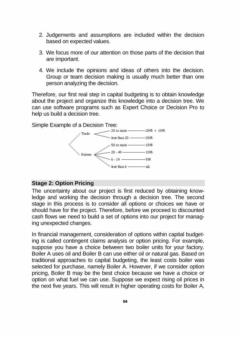
54

2. Judgements and assumptions are included within the decision based on expected values.

3. We focus more of our attention on those parts of the decision that are important.

4. We include the opinions and ideas of others into the decision. Group or team decision making is usually much better than one person analyzing the decision.

Therefore, our first real step in capital budgeting is to obtain knowledge about the project and organize this knowledge into a decision tree. We can use software programs such as Expert Choice or Decision Pro to help us build a decision tree.

Simple Example of a Decision Tree:

Stage 2: Option Pricing

The uncertainty about our project is first reduced by obtaining know-ledge and working the decision through a decision tree. The second stage in this process is to consider all options or choices we have or should have for the project. Therefore, before we proceed to discounted cash flows we need to build a set of options into our project for manag-ing unexpected changes.

In financial management, consideration of options within capital budget-ing is called contingent claims analysis or option pricing. For example, suppose you have a choice between two boiler units for your factory. Boiler A uses oil and Boiler B can use either oil or natural gas. Based on traditional approaches to capital budgeting, the least costs boiler was selected for purchase, namely Boiler A. However, if we consider option pricing, Boiler B may be the best choice because we have a choice or option on what fuel we can use. Suppose we expect rising oil prices in the next five years. This will result in higher operating costs for Boiler A,

55

but Boiler B can switch to a second fuel to better control operating costs. Consequently, we want to assess the options of capital projects.

Options can take many forms; ability to delay, defer, postpone, alter, change, etc. These options give us more opportunities for creating value within capital projects. We need to think of capital projects as a bundle of options. Three common sources of options are:

1. Timing Options: The ability to delay our investment in the project.

2. Abandonment Options: The ability to abandon or get out of a project that has gone bad.

3. Growth Options: The ability of a project to provide long-term growth despite negative values. For example, a new research program may appear negative, but it might lead to new product innovations and market growth. We need to consider the growth options of projects.

Option pricing is the additional value that we recognize within a project because it has flexibilities over similar projects. These flexibilities help us manage capital projects and therefore, failure to recognize option values can result in an under-valuation of a project.

Stage 3: Discounted Cash Flows

So we have completed the first two stages of capital budgeting analysis: (1) Build and organize knowledge within a decision tree and (2) Recog-nize and build options within our capital projects. We can now make an investment decision based on Discounted Cash Flows or DCF.

Unlike accounting, financial management is concerned with the values of assets today; i.e. present values. Since capital projects provide bene-fits into the future and since we want to determine the present value of the project, we will discount the future cash flows of a project to the present.

Discounting refers to taking a future amount and finding its value today. Future values differ from present values because of the time value of money. Financial management recognizes the time value of money be-cause:

1. Inflation reduces values over time; i.e. $1,000 today will have less value five years from now due to rising prices (inflation).

56

2. Uncertainty in the future; i.e. we think we will receive $1,000 five years from now, but a lot can happen over the next five years.

3. Opportunity Costs of money; $1,000 today is worth more to us than $1,000 five years from now because we can invest $1,000 today and earn a return.

One way present values are calculated is by referring to tables. The dis-count rate we will use is the opportunity costs of the investment; i.e. the rate of return we require on any other project with similar risks.

EXHIBIT 1 — Present Value of $1.00, year = n, rate = k Year (n) k = 10% k = 11% k = 12%

1 0.909 0.901 0.893 2 0.826 0.812 0.797 3 0.751 0.731 0.712 4 0.683 0.659 0.636 5 0.621 0.593 0.567

EXAMPLE 1 — Calculate the Present Value of Cash Flows You will receive $500 at the end of next year. If you could invest the $500 today, you estimate that you could earn 12%. What is the Present Value of this future cash inflow? $500 x 0.893 (Exhibit 1) = $446.50

If we were to receive the same cash flows year after year in the future, then we could use the present value tables for an annuity.

EXHIBIT 2 — Present Value of Annuity for $1.00, year = n, rate = k Year (n) k = 10% k = 11% k = 12% 1 0.909 0.901 0.893 2 1.736 1.713 1.690 3 2.487 2.444 2.402 4 3.170 3.102 3.037 5 3.791 3.696 3.605

EXAMPLE 2 — Calculate the Present Value of Annuity Type Cash Flows You will receive $500 each year for the next five years. Your opportuni-ty costs for this investment is 10%. What is the present value of this in-vestment?

57

$500 x 3.791 (Exhibit 2) = $1,895.50

Another way to calculate Present values of future cash flows is using fi-nancial formula:

ti

FVPV

)1(

where

PV – Present Value of Cash Flows

FV – Future Value of Cash Flows

i – Discount rate for the period

t – Period under review

In case of annuity we may use the following financial formula to calcu-late present value of future cash flows:

n

t

tnAi

PMTPV

1 )1(

1

,

Where

PVA – Present Value of Annuity

PMT – Annuity Payment

n – Number of periods

i – Discount rate for the period

t – Period under review

We now understand discounting of cash flows (DCF) and the three rea-sons why we discount future cash flows: Inflation, Uncertainty, and Op-portunity Costs.

58

Chapter 2: Calculating the Discounted Cash Flows of Projects

In capital budgeting analysis we want to determine the after tax cash flows associated with capital projects. We are concerned with all rele-vant changes or differences in cash flows once we invest in the project.

Understanding "Relevancy"

One question that we must ask in capital budgeting is what is relevant. Here are some examples of what is relevant to project cash flows:

1. Depreciation: Capital assets are subject to depreciation and we need to account for depreciation twice in our calculations of cash flows. We deduct depreciation once to calculate the taxes we pay on project revenues and we add back depreciation to arrive at cash flows be-cause depreciation is a non-cash item.

2. Working Capital: Major investments may require increases to working capital. For example, new production facilities often require more in-ventories and higher salaries payable. Therefore, we need to consid-er the net change in working capital associated with our project. Changes in net working capital will sometimes reverse themselves at the end of the project.

3. Overhead: Many capital projects can result in increases to allocated overheads, such as computer support services. However, the subjec-tive nature of overhead allocations may not make any difference at all. Therefore, you need to assess the impact of your capital project on overhead and determine if these costs are relevant.

Financing Costs: If we plan on financing a capital project, this will involve additional cash flows to investors. The best way to account for financing costs is to include them within our discount rate. This eliminates the possibility of double-counting the financing costs by deducting them in our cash flows and discounting at our cost of capital which also includes our financing costs. We also need to ignore costs that are sunk; i.e. costs that will not change if we invest in the project. For example, a new product line may require some preliminary marketing research. This research is done re-

59

gardless of the project and thus, it is sunk. The concept of sunk costs and relevant costs applies to all types of financing decisions.

EXAMPLE 3 — Make or Buy Decision You have the option to manufacture your own parts or purchase them from outside suppliers. If we purchase the parts, it will cost $50.00 per part. Our factory is operating at 70% of capacity and our total costs to manufacture parts is: Direct Materials $15.00 / part Direct Labor $19.00 / part Overhead - Variable $14.00 / part Overhead - Fixed $12.00 / part Total Costs $60.00 / part Since we are operating at 70% capacity, we do not expect an increase in fixed overhead; this is a sunk cost. We would manufacture the parts since it is $2.00 / part cheaper: Purchase $50.00 vs. Manufacture $48.00 ($15.00 + $19.00 + $14.00)

EXAMPLE 4 — Discontinue a Product You are considering dropping product GX-4 from your product line be-cause the Income Statement for GX-4 shows the following: Traditional Relevant Sales Revenues $10,000 $10,000 Cost of Goods Sold - Variable ( 6,000) ( 6,000) Cost of Goods Sold - Fixed ( 2,000) Operating Expenses - Variable ( 2,500) (2,500) Operating Expenses - Fixed ( 600) Income (Loss) $( 1,100) $1,500 Conclusion: We should continue selling GX-4 since it earns $1,500 of Income.

EXAMPLE 5 — Accept a Special Offer A customer has offered you $15.00 for 5,000 units of your product. You normally sell your product for $25.00. Should you accept this of-fer? You currently produce and sell 40,000 units with a maximum capacity of 50,000 units. Total manufacturing costs are $18.00 per unit, consist-ing of $12.50 variable and $5.50 fixed.

60

Change in Revenues $75,000 (5,000 x $15.00) Change in Expenses ( 62,500) (5,000 x $12.50) Net Change $12,500 Conclusion: You should accept the special offer since it results in $12,500 of additional income.

So far, we have covered present values and relevancy within capital budgeting. We now can proceed to calculate the present value of rele-vant cash flows. Once we have determined the present value of cash flows, we will have a basis for comparing our initial investment. Both values (future cash flows and initial investment) will be expressed in cur-rent values. The net of these two amounts will tell us how much value we will create or destroy by investing in a project.

EXAMPLE 6 — Calculate Relevant Cash Flows for Capital Project We plan on purchasing a new assembly machine for $25,000.. It will cost $2,000 to have the new machine installed and we expect a $1,000 net increase in working capital. By making the investment, we will reduce our annual operating costs by $7,000 and we expect to save $500 a year in maintenance. The new machine will require $750 each year for technical support. We will depreciate the machine over 5 years under the straight-line method of depreciation with an expected salvage value of $5,000. The effective tax rate is 35%. Annual Savings in Operating Costs $7,000 Annual Savings in Maintenance 500 Annual Costs for Technical Support ( 750) Annual Depreciation ( 4,000) * Revenues $2,750 Taxes @ 35% ( 962) Net Project Income 1,788 Add Back Depreciation (noncash item) 4,000 Relevant Project Cash Flow $5,788 * $25,000 - $5,000 / 5 years = $4,000

We will receive $5,788 of cash flow each year by investing in this new assembly machine. Since we have a salvage value, we have a terminal cash flow associated with this project.

EXAMPLE 7 — Calculate Terminal Cash Flow for Capital Project Estimated Salvage Amount in 5 Years $5,000 Less Taxes (1,750)

61

Terminal Cash Flow $3,250

Calculating the Present Value of Cash Flows

Our next step is to calculate present values of our two cash flow streams. We will use our cost of capital to discount the cash flows. We will assume that our cost of capital is 12%. We will use the present value tables in Exhibits 1 and 2 for finding the appropriate discount factor per the life of our cash streams and the 12% cost of capital.

EXAMPLE 8 — Calculate Present Value of Cash Flows Annual Project Cash Flows $5,788 Discount Factor per Exhibit 2 x 3.605 (1) Present Value of Annual Flows $20,866 Terminal Cash Flow $3,250 Discount Factor per Exhibit 1 x 0.567 (2) Present Value of Terminal Flow 1,843 Total Present Value $22,709 (1): We use the Annuity Table since we have the same cash flows each year for the next 5 years. If we look at Exhibit 2 for n = 5 years and 12%, we find 3.605 (2): We need to discount the terminal cash flow received five years from now to the present by using the Present Value Table in Exhibit 1.

Calculating Net Investment

Now that we have the current value of $22,709 for our cash flows, we need to compare this to our investment amount. Our investment is the total cash outlay we must make today and it includes:

1. All cash paid out to invest in the project and place it into service, such as installation, transportation, etc.

2. Net proceeds from the disposal of any old equipment that will be re-placed by the new equipment.

3. Any taxes paid and/or tax benefits received from making the invest-ment.

EXAMPLE 9 — Calculate Net Investment

62

Referring back to Example 6, we can calculate our Net Investment. We will also assume that an existing machine can be sold for $6,000. Acquisition Costs $25,000 Installation Costs 2,000 Increase in Working Capital 1,000 Proceeds from Sale $(6,000) Less Taxes @ 35% (2,100) Net Proceeds from Sale (3,900) Net Investment $24,100

So we now have a current value for our cash flows of $22,709 and a to-tal net investment of $24,100. These amounts are derived by looking at three different types of cash flows:

1. Relevant cash flows during the life of the project. 2. Terminal cash flows at the end of the project. 3. Initial cash flows (net investment).

Chapter 3: Three Economic Criteria for Evaluating Capi-tal Projects

We have completed our three main stages of capital budgeting analysis, including the calculation of discounted cash flows. The next step is to apply some economic criteria for evaluating the project. We will use three criteria: Net Present Value, Modified Internal Rate of Return, and Discounted Payback Period.

Net Present Value

The first criterion we will use to evaluate capital projects is Net Present Value. Net Present Value (NPV) is the total net present value of the project. It represents the total value added or subtracted from the organ-ization if we invest in this project. We can refer back to our previous ex-ample and calculate Net Present Value.

EXAMPLE 10 — Calculate Net Present Value Net Investment Outflow (Example 9) $(24,100) Present Value of Inflows (Example 8) 22,709 Net Present Value $(1,391)

63

If the Net Present Value is positive, we should proceed and make the investment. If the Net Present Value is negative (as is the case in Ex-ample 10), then we would not make the investment.

Modified Internal Rate of Return

Besides determining the Net Present Value of a project, we can calcu-late the rate of return earned by the project. This is called the Internal Rate

of Return. Internal Rate of Return (IRR) is one of the most popular eco-nomic criteria for evaluating capital projects since managers can identify with rates of return. Internal Rate of Return is calculated by finding the discount rate whereby the Net Investment amount equals the total present value of all cash inflows; i.e. Net Present Value = 0. If we have equal cash inflows each year, we can solve for IRR easily.

EXAMPLE 11 — Calculate Internal Rate of Return Referring back Example 6, we would solve for IRR as follows: $5,788 x discount factor = $24,100 or $24,100 / $5,788 = 4.164. If we look in the Present Value Tables for n = 5 years, we want to find a present value factor nearest to 4.164. By referring to pub-lished present value tables, we find the following: At 6%, n = 5 4.2124 4.2124 As Calculated 4.1640 At 7%, n = 5 4.1002 Difference 0.0484 0.1122 0.06 + ( 0.0484 / 0.1122) x (0.07 - 0.06) = 0.0643 Internal Rate of Return = 6.43%

If the Internal Rate of Return were higher than our cost of capital, then we would accept this project. In our example, the IRR (6.43%) is less than our cost of capital (12%). Therefore, we would not invest in this project.

One of the problems with IRR is the so-called reinvestment rate as-sumption. IRR makes the assumption that every year you will be able to earn the IRR each time you reinvest your cash inflows. This assumption can result in some major distortions between Net Present Value and In-

64

ternal Rate of Return. We will correct this distortion by modifying our IRR calculation.

EXAMPLE 12 — IRR Distortions from Reinvestment Rate Assump-tion A summary of four simple projects with IRR and NPV:

Cash Inflows Project Investment Year-1 Year-2 IRR NPV

A $2,000 $0 $4,500 50% $3,130 B 2,000 1,500 2,250 50% 2,810 C 2,000 2,450 1,000 55% 2,640 D 2,000 0 4,210 45% 2,940

If we use IRR, we would select Project C, but if we go by NPV, we would select Project A.

In order to eliminate the reinvestment rate assumption, we will modify the Internal Rate of Return so that the reinvestment rate is our cost of capital. This will give us a more accurate IRR for our project. Fortunate-ly, we can use spreadsheets like Microsoft Excel to calculate Modified Internal Rate of Return.

EXAMPLE 13 — Calculate Modified IRR Using Microsoft Excel Referring back to Example 6, we have the following: $5,788 annual project cash inflows $24,100 net investment amount 12% cost of capital The formula for calculating Modified IRR in a Microsoft Excel Spreadheet is: @MIRR(A1:An, k%, r%) A1:An is the cell range for entering our data. We always enter the net investment in the first cell and the cash inflows in each cell the-reafter. k% refers to our cost of capital and r% is the rate we believe we can earn when we reinvest cash inflows. If we assume that we can earn our cost of capital on reinvested cash flows, then we would enter the following from our example: Cell Input Output A1 -24,100 A2 5,788 A3 5,788

65

A4 5,788 A5 5,788 A6 5,788 B1@MIRR(A1:A6, 12%, 12%) 9% The Modified IRR on our project is 9%.

Discounted Payback Period

The final economic criteria we will use is the Discounted Payback Pe-riod. Payback refers to the number of years it takes to recover our net investment. In our previous example (Example 6), we could use a sim-ple payback calculation as follows:

$24,100 / $5,788 = 4.2 years

However, this method does not recognize the time value of money and as we previously indicated, we must consider the time value of money because of inflation, uncertainty, and opportunity costs. Therefore, we will use the discounted cash flows to calculate the payback period (dis-counted payback period).

EXAMPLE 14 — Calculate Discounted Payback Period Referring back to Example 6, we can calculate the discounted pay-back period as follows: Year Cash Flow x P.V. Factor = P.V. Cash Flow Total to Date 1 $5,788 0.893 $5,169 $5,169 2 5,788 0.797 4,613 9,782 3 5,788 0.712 4,121 13,903 4 5,788 0.636 3,681 17,584 5 5,788 0.567 3,282 20,866 5 3,250 0.567 1,843 22,709

Under the Discounted Payback Period, we would never receive a pay-back on our project; i.e. the total to date present cash flows never reached $24,100 (net investment). If we had relied on the regular pay-back calculation, we would falsely assume that this project does pay-back in the fourth year.

In summary, we use economic criteria that have realistic economic as-sumptions about capital investments. Three economic criteria that meet this test are:

66

1) Net Present Value

2) Modified Internal Rate of Return

3) Discounted Payback Period

Chapter 4: Additional Considerations in Capital Budget-ing Analysis

Whenever we analyze a capital project, we must consider unique fac-tors. A discussion of all of these factors is beyond the scope of this course. However, three common factors to consider are:

Compensating for different levels of risks between projects. Recognizing risks that are specific to foreign projects. Making adjustments to capital budgeting analysis by looking at the ac-tual results.

Adjusting for Risk

We previously learned that we can manage uncertainty by initiating de-cision analysis and building options into our projects. We now want to turn our attention to managing risks. It is worth noting that uncertainty and risk are not the same thing. Uncertainty is where you have no basis for a decision. Risk is where you do have a basis for a decision, but you have the possibility of several outcomes. The wider the variation of out-comes, the higher the risk.

In our previous example (Example 6), we used the cost of capital for discounting cash flows. Our example involved the replacement of equipment and carried a low level of risk since the expected outcome was reasonably certain. Suppose we have a project involving a new product line. Would we still use our cost of capital to discount these cash flows? The answer is "NO" since this project could have a much wider variation in outcomes. We can adjust for higher levels of risk by increas-ing the discount rate. A higher discount rate reflects a higher rate of re-turn that we require whenever we have higher levels of risk.

Another way to adjust for risk is to understand the impact of risk on out-comes. Sensitivity Analysis and Simulation can be used to measure how changes to a project affect the outcome. Sensitivity analysis is used to determine the change in Net Present Value given a change in a spe-cific variable, such as estimated project revenues. Simulation allows us to simulate the results of a project for a given distribution of variables. Both sensitivity analysis and simulation require a definition of all relevant

67

variables associated with the project. It should be noted that sensitivity analysis is much easier to implement since sophisticated computer models are usually required for simulation.

International Projects

Capital investments in other countries can involve additional risks. Whenever we invest in a foreign project, we want to focus on the values that are added (or subtracted) to the Parent Company. This makes us consider all relevant risks of the project, such as exchange rate risk, po-litical risk, hyper-inflation, etc. For example, the discounted cash flows of the project are the discounted cash flows of the project to the foreign subsidiary converted to the currency of the home country of the Parent Company at the current exchange rate. This forces us to take into ac-count exchange rate risks and its impact to the Parent Company.

Post Analysis

One of the most important steps in capital budgeting analysis is to fol-low-up and compare your estimates to actual results. This post analysis or review can help identify bias and errors within the overall process. A formal tracking system of capital projects also keeps everyone honest. For example, if you were to announce to everyone that actual results will be tracked during the life of the project, you may find that people who submit estimates will be more careful. The purpose of post analysis and tracking is to collect information that will lead to improvements within the capital budgeting process.

Chapter 5: Course Summary

The long-term investments we make today determines the value we will have tomorrow. Therefore, capital budgeting analysis is critical to creat-ing value within financial management. And the only certainty within capital budgeting is uncertainty. Therefore, one of the biggest chal-lenges in capital budgeting is to manage uncertainty. We deal with un-certainty through a three-stage process: Build knowledge through decision analysis. Recognize and encourage options within projects. Invest based on economic criteria that have realistic economic assump-tions.

68

Once we have completed the three-stage process (as outlined above), we evaluate capital projects using a mix of economic criteria that ad-heres to the principles of financial management. Three good economic criteria are Net Present Value, Modified Internal Rate of Return, and Discounted Payback.

Additionally, we need to manage project risk differently than we would manage uncertainty. We have several tools to help us manage risks, such as increasing the discount rate. Finally, we want to implement post analysis and tracking of projects after we have made the investment. This helps eliminate bias and errors in the capital budgeting process.

69

Terminology Section III: Capital Budgeting Analysis

Chapter 1

Capital budgeting ......................... = 1) Составление смет капи-тальных вложений и их оку-паемости 2) Экономический анализ на-мечаемых капитальных вло-жений (Анализ капвложений).

Expansion .................................... = Расширение Outlays ........................................ = expenses, costs To commit to ................................ = брать на себя обязательства To back out .................................. = отказаться от участия, укло-

ниться Present Value .............................. = настоящая, текущая стои-

мость Discounted Cash Flow (DCF) ...... = Дисконтированный поток на-

личности Decision Analysis ......................... = Анализ принятия решений Option Pricing .............................. = Стоимостная оценка вариан-

тов Complex....................................... = hard, combined = сложный, со-

ставной Outcome ...................................... = result, consequence = резуль-

тат, последствие, исход Tax considerations ....................... = Оплата / возмещение налогов Disposal Value ............................. = Salvage, Residual Value = оста-

точная стоимость Capacity Utilization ...................... = Использование производст-

венных мощностей Consequently ............................... = Therefore, hence = Поэтому,

следовательно Hierarchy ..................................... = Subordination system = Иерар-

хия Attribute ....................................... = Свойство, признак, характер-

ная черта, характеристика To derive ...................................... = to obtain, to draw, to get = полу-

чать, извлекать

70

Contingent claims analysis ........... = Анализ вероятных (случайных) требований

To defer ....................................... = to delay, to postpone, to put off To alter ........................................ = to change Bundle ......................................... = связка, вязанка, пучок, пакет,

большое количество Timing options ............................. = Временные возможности Abandonment options .................. = Возможности отказа Growth options ............................. = Возможности для роста Option Values .............................. = возможные выгоды Time value of money .................... = Временная стоимость денег Opportunity Costs (Losses) .......... = Издержки (потери) вследствие

не использования благоприят-ных возможностей.

Annuity ......................................... = Аннуитет

Chapter 2

Relevancy .................................... = appropriateness = значимость, существенность, уместность

Working capital ............................ = оборотные средства, оборот-ный капитал

Allocated Overheads .................... = выделенные накладные рас-ходы

Sunk Costs .................................. = невозвратные издержки Net ............................................... = (экон.) сальдо, нетто Assembly machine ....................... = Сборочный агрегат Present Value .............................. = настоящая (текущая) стои-

мость Salvage value .............................. = Ликвидационная стоимость Terminal Cash flow ...................... = конечный, заключительный

поток наличности Net proceeds ............................... = чистый доход, вырученная

сумма

Chapter 3

Net Present Value ........................ = Чистая приведенная стои-мость

Internal Rate of Return ................. = Внутренняя норма прибыль-ности (рентабельности) проек-та

Criterion ....................................... = Признак, критерий

71

To refer ........................................ = обращаться к чему-либо, ссы-латься на что-либо

To eliminate ................................. = to remove, to expel = устранять, исключать, ликвидировать

Discounted Payback .................... = Дисконтированная окупае-мость

Discounted rate ............................ = Ставка дисконтирования

Chapter 4

Consideration ............................... = Суждение, размышление, взгляд, мнение

Scope .......................................... = Границы, рамки, пределы Uncertainty ................................... = Where you have no basis for a

decision Risk .............................................. = Where you have a basis for a

decision, but you have a possi-bility of several outcomes

Bias .............................................. = Отклонение, сдвиг, тенденция Improvement ................................ = Улучшение, усовершенство-

вание Mix ............................................... = Набор To adhere .................................... = Прилипать, придерживаться

72

Questions Section III: Capital Budgeting Analysis

NOTE: The following questions are based on the material of the section and imply answers in a form of discussion

1. What is Capital Expenditure?

2. What is the purpose of Capital Budgeting Analysis (CBA)?

3. What are the Three Stages of Capital Budgeting Analysis?

4. Which stage of CBA implies the greatest level of uncertainty?

5. Which stage of CBA demands greater investment amount?

6. What is a Decision Tree and what is its purpose in the Decision Analysis?

7. What is the purpose of Decision Analysis in the CBA?

8. What is the purpose of Option Pricing in the CBA?

9. What is timing options in the option pricing stage if CBA?

10. What is abandonment options in the option pricing stage of CBA?

11. How would you explain what Discounted Cash Flows mean?

12. What are some of the things that we need to take into considera-tions when calculating DCF?

73

True or False Section III: Capital Budgeting Analysis

Mark the following statements True if you agree with it or False if you don’t agree with the statement?

1. When you acquire new technologies for production it can NOT be considered as capital expenditure. __________

2. Capital Budgeting Analysis helps us to answer the question wheth-er future benefits of a project will be large enough to justify the in-vestment given the risk involved. ___________

3. Multiple Attribute Decision Model (MADM) is another name for De-cision Tree. ___________

4. A Decision Tree helps us to break complex questions down to a number of simple ones. ___________

5. Timing Options include the ability to alter the project. ___________

6. Opportunity Costs are expenses that you undertake to use an op-portunity of investing in the project ___________

7. Relevancy helps us understand and determine which cash flows are connected with the project and which don’t depend on it. ____________

8. Present Value of Cash Flow shows its value when you receive it. ____________

9. Net Present Value is the difference between Present Value of In-flows and Net Investment Outflows. ____________

10. Internal Rate of Return helps us identify the profitability of the project. ____________

74

Sources and References

1. Financial Management: Theory and Practice by Eugene F. Brig-ham, Michael C. Ehrhardt, South-Western College Pub; 10th edi-tion (August 3, 2001) 1136 pages.

2. Fundamentals of Financial Management: Concise Edition by Eu-gene F. Brigham, Joel F. Houston, South-Western College Pub; 3rd edition (July 9, 2001), 688 pages.

3. Multinational Financial Management by Alan C. Shapiro, John Wi-ley & Sons; 7th edition (May 2002), 848 pages.

4. Колб Р.В., Родригес П.Дж. Финансовый менеджмент: учебник / пер. 2-го английского издания, - М.: издательство"Финпресс", 2001. – 496 с.

5. Ван Хорн, Джеймс К., Вахович, мл.Джон. М. Основы финансо-вого менеджмента, 11-ое издание: пер. с англ. – М.: Изда-тельский дом "Вильямс", 2001. – 992 с.

6. Крейнина М.Н. Финансовый менеджмент / Учебное пособие. – М.: Издательство "Дело и Сервис", 1998. – 304 с.

7. Лялин В.А., Воробьев П.В. Финансовый менеджмент: Учебное пособие. – 2-е изд., испр. и доп. – СПб.: "Бизнес-пресса", 2001. – 144 с.

8. Бендина Н. Финансовый менеджмент (конспект лекций). – М.: "Издательство ПРИОР", 2002. – 144 с.

75

Timur R. Rakhimov

Financial Management

Textbook

Edited by: R.I. Tolbanova