SECTION 6.2: VOLUMES OF SOLIDS OF …Section 6.2: Volumes of Solids of Revolution: Disk / Washer Methods) 6.2.2 It helps that the axis of revolution does not pass through the interior

(Section 6.2: Volumes of Solids of Revolution: Disk / Washer Methods) 6.2.1

SECTION 6.2: VOLUMES OF SOLIDS OF REVOLUTION: DISK / WASHER METHODS

LEARNING OBJECTIVES

• Find volumes of solids of revolution using Disk and Washer Methods. • Prove formulas for volumes of cones, spheres, etc. PART A: THE DISK METHOD (“dx SCAN”)

A solid of revolution is obtained by revolving a plane (flat) region, called a generating region, about an axis of revolution. The Disk and Washer Methods can be used to find the volume of such a solid. Example 1 (Finding a Volume Using the Disk Method: “dx Scan”)

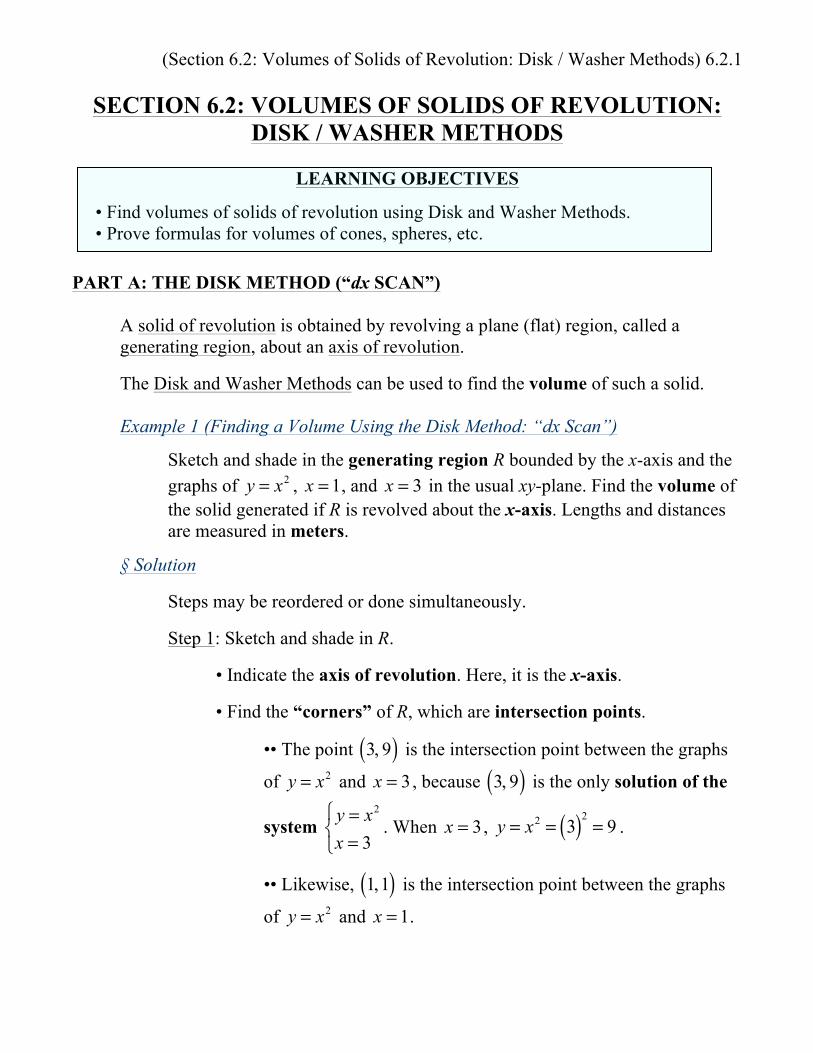
Sketch and shade in the generating region R bounded by the x-axis and the graphs of y = x2 , x = 1, and x = 3 in the usual xy-plane. Find the volume of the solid generated if R is revolved about the x-axis. Lengths and distances are measured in meters.

§ Solution Steps may be reordered or done simultaneously. Step 1: Sketch and shade in R.

• Indicate the axis of revolution. Here, it is the x-axis.

• Find the “corners” of R, which are intersection points.

•• The point 3, 9( ) is the intersection point between the graphs

of y = x2 and x = 3 , because 3, 9( ) is the only solution of the

system

y = x2

x = 3⎧⎨⎩

. When x = 3 , y = x2 = 3( )2= 9 .

•• Likewise, 1,1( ) is the intersection point between the graphs

of y = x2 and x = 1.


It helps that the axis of revolution does not pass through the interior of R. See Example 2.

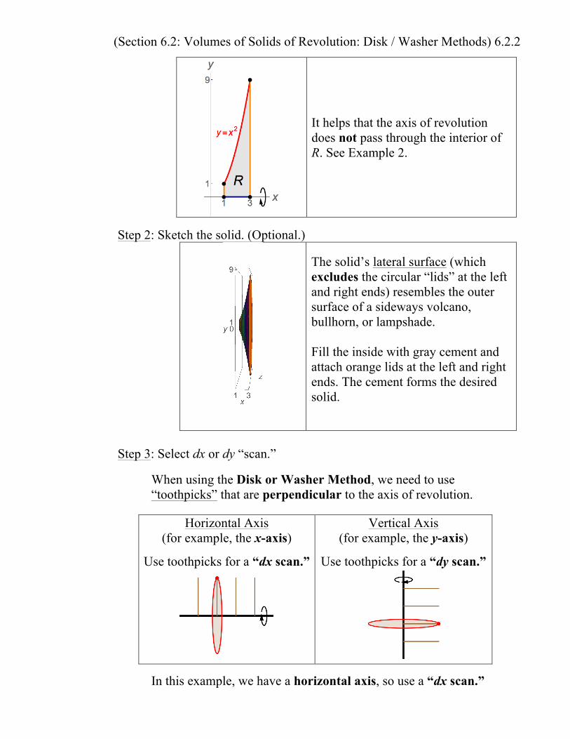
Step 2: Sketch the solid. (Optional.)

The solid’s lateral surface (which excludes the circular “lids” at the left and right ends) resembles the outer surface of a sideways volcano, bullhorn, or lampshade. Fill the inside with gray cement and attach orange lids at the left and right ends. The cement forms the desired solid.

Step 3: Select dx or dy “scan.”

When using the Disk or Washer Method, we need to use “toothpicks” that are perpendicular to the axis of revolution.

Horizontal Axis

(for example, the x-axis)

Use toothpicks for a “dx scan.”

Vertical Axis (for example, the y-axis)

Use toothpicks for a “dy scan.”

In this example, we have a horizontal axis, so use a “dx scan.”


Step 4: Rewrite equations (if necessary).

Consider the equations of the boundaries of R that have both x and y in them. • For a “dx scan,” solve them for y in terms of x. • For a “dy scan,” solve them for x in terms of y.

In this example, we are doing a “dx scan,” so the equation y = x2 is

fine as-is. It is already solved for y in terms of x.

Step 5: Find the area of [one face of] a cross section.

• Fix a representative, generic x-value in 1, 3( ) .

(We could have said 1, 3⎡⎣ ⎤⎦ in this example.)

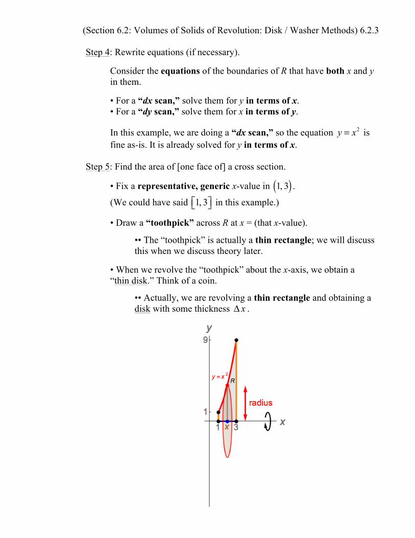
• Draw a “toothpick” across R at x = (that x-value).

•• The “toothpick” is actually a thin rectangle; we will discuss this when we discuss theory later.

• When we revolve the “toothpick” about the x-axis, we obtain a “thin disk.” Think of a coin.

•• Actually, we are revolving a thin rectangle and obtaining a disk with some thickness Δ x .

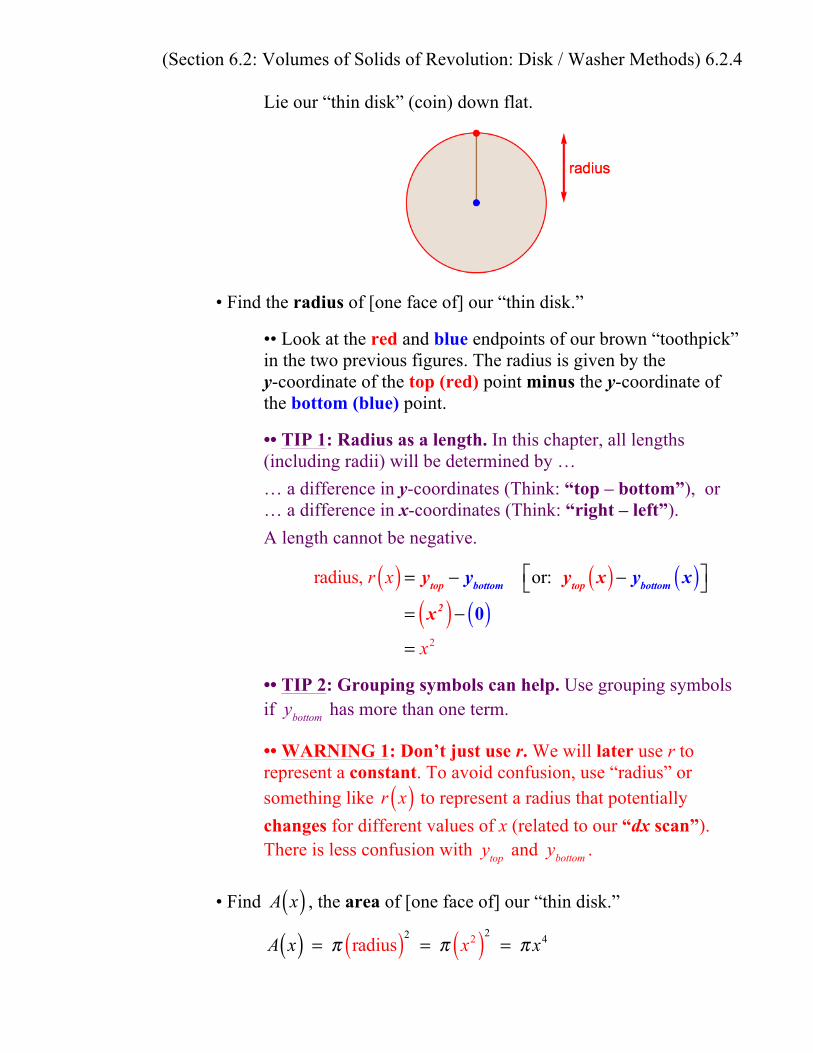
(Section 6.2: Volumes of Solids of Revolution: Disk / Washer Methods) 6.2.4 Lie our “thin disk” (coin) down flat.

• Find the radius of [one face of] our “thin disk.”

•• Look at the red and blue endpoints of our brown “toothpick” in the two previous figures. The radius is given by the y-coordinate of the top (red) point minus the y-coordinate of the bottom (blue) point. •• TIP 1: Radius as a length. In this chapter, all lengths (including radii) will be determined by …

… a difference in y-coordinates (Think: “top – bottom”), or … a difference in x-coordinates (Think: “right – left”).

A length cannot be negative.

radius, r x( ) = ytop − ybottom or: ytop x( )− ybottom x( )⎡⎣ ⎤⎦= x2( )− 0( )= x2

•• TIP 2: Grouping symbols can help. Use grouping symbols if ybottom has more than one term.

•• WARNING 1: Don’t just use r. We will later use r to represent a constant. To avoid confusion, use “radius” or something like r x( ) to represent a radius that potentially changes for different values of x (related to our “dx scan”). There is less confusion with

ytop

and

ybottom .

• Find A x( ) , the area of [one face of] our “thin disk.”

A x( ) = π radius( )2= π x2( )2

= π x4


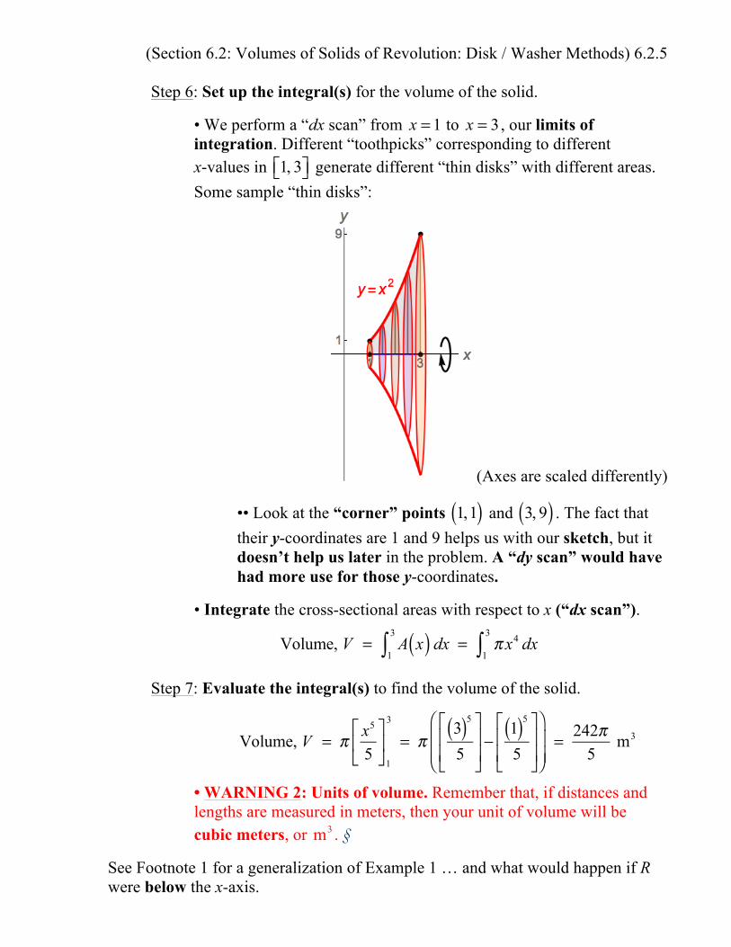
Step 6: Set up the integral(s) for the volume of the solid.

• We perform a “dx scan” from x = 1 to x = 3 , our limits of integration. Different “toothpicks” corresponding to different x-values in 1, 3⎡⎣ ⎤⎦ generate different “thin disks” with different areas. Some sample “thin disks”:

(Axes are scaled differently)

•• Look at the “corner” points 1,1( ) and 3, 9( ) . The fact that their y-coordinates are 1 and 9 helps us with our sketch, but it doesn’t help us later in the problem. A “dy scan” would have had more use for those y-coordinates.

• Integrate the cross-sectional areas with respect to x (“dx scan”).

Volume, V = A x( ) dx

1

3

∫ = π x4 dx1

3

∫

Step 7: Evaluate the integral(s) to find the volume of the solid.

Volume, V = π x5

5⎡

⎣⎢

⎤

⎦⎥

1

3

= π3( )5

5

⎡

⎣⎢⎢

⎤

⎦⎥⎥−

1( )5

5

⎡

⎣⎢⎢

⎤

⎦⎥⎥

⎛

⎝⎜⎜

⎞

⎠⎟⎟= 242π

5 m3

• WARNING 2: Units of volume. Remember that, if distances and lengths are measured in meters, then your unit of volume will be cubic meters, or m3 . §

See Footnote 1 for a generalization of Example 1 … and what would happen if R were below the x-axis.

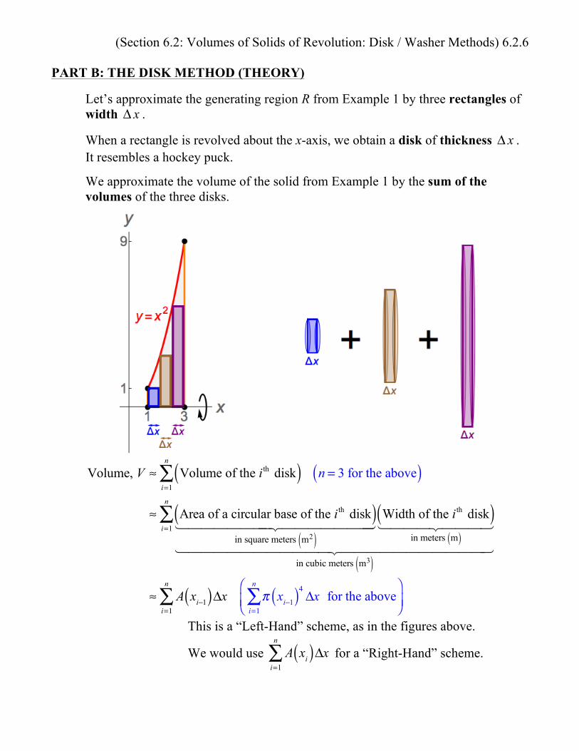
(Section 6.2: Volumes of Solids of Revolution: Disk / Washer Methods) 6.2.6 PART B: THE DISK METHOD (THEORY)

Let’s approximate the generating region R from Example 1 by three rectangles of width Δ x .

When a rectangle is revolved about the x-axis, we obtain a disk of thickness Δ x . It resembles a hockey puck.

We approximate the volume of the solid from Example 1 by the sum of the volumes of the three disks.

Volume, V ≈ Volume of the i th disk( )i=1

n

∑ n = 3 for the above( )

≈ Area of a circular base of the i th disk( )in square meters m2( )

Width of the i th disk( )

in meters m( )

in cubic meters m3( )

i=1

n

∑

≈ A xi−1( )Δxi=1

n

∑ π xi−1( )4Δx

i=1

n

∑ for the above⎛

⎝⎜⎞

⎠⎟

This is a “Left-Hand” scheme, as in the figures above.

We would use

A xi( )Δxi=1

n

∑ for a “Right-Hand” scheme.


To get the exact volume, let Δ x → 0 . For regular partitions, this implies that P → 0 .

Volume, V = limP → 0

A xi−1( )Δ xi=1

n

∑ limP → 0

π xi−1( )4Δ x

i=1

n

∑ for Example 1⎛

⎝⎜⎞

⎠⎟

= A x( ) dxa

b

∫ π x4 dx1

3

∫ for Example 1⎛⎝

⎞⎠

assuming A is a continuous function on a, b⎡⎣ ⎤⎦ .

Δ x is replaced by dx in the integral. PART C: THE DISK METHOD (“dy SCAN”)

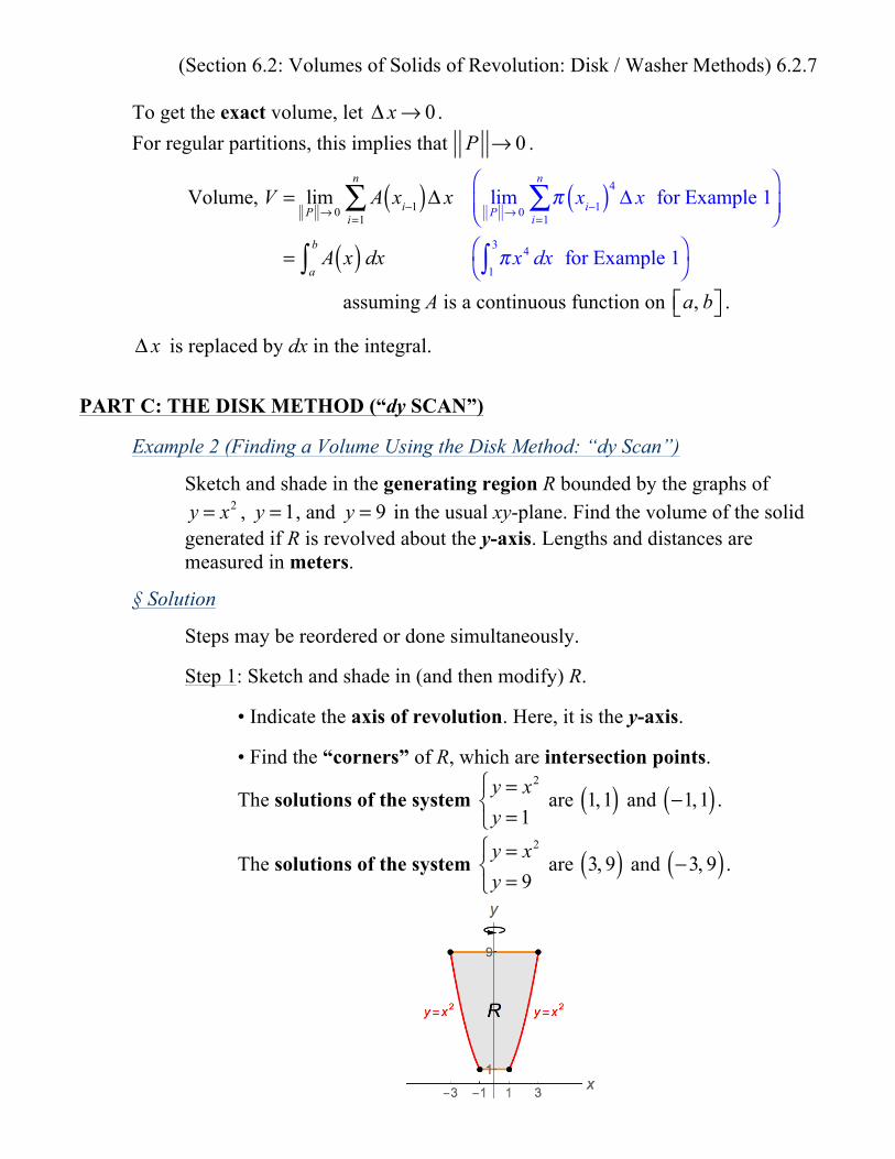
Example 2 (Finding a Volume Using the Disk Method: “dy Scan”)

Sketch and shade in the generating region R bounded by the graphs of

y = x2 , y = 1, and y = 9 in the usual xy-plane. Find the volume of the solid generated if R is revolved about the y-axis. Lengths and distances are measured in meters.

§ Solution

Steps may be reordered or done simultaneously. Step 1: Sketch and shade in (and then modify) R.

• Indicate the axis of revolution. Here, it is the y-axis.

• Find the “corners” of R, which are intersection points.

The solutions of the system

y = x2

y = 1⎧⎨⎩

are 1,1( ) and −1,1( ) .

The solutions of the system

y = x2

y = 9⎧⎨⎩

are 3, 9( ) and −3, 9( ) .


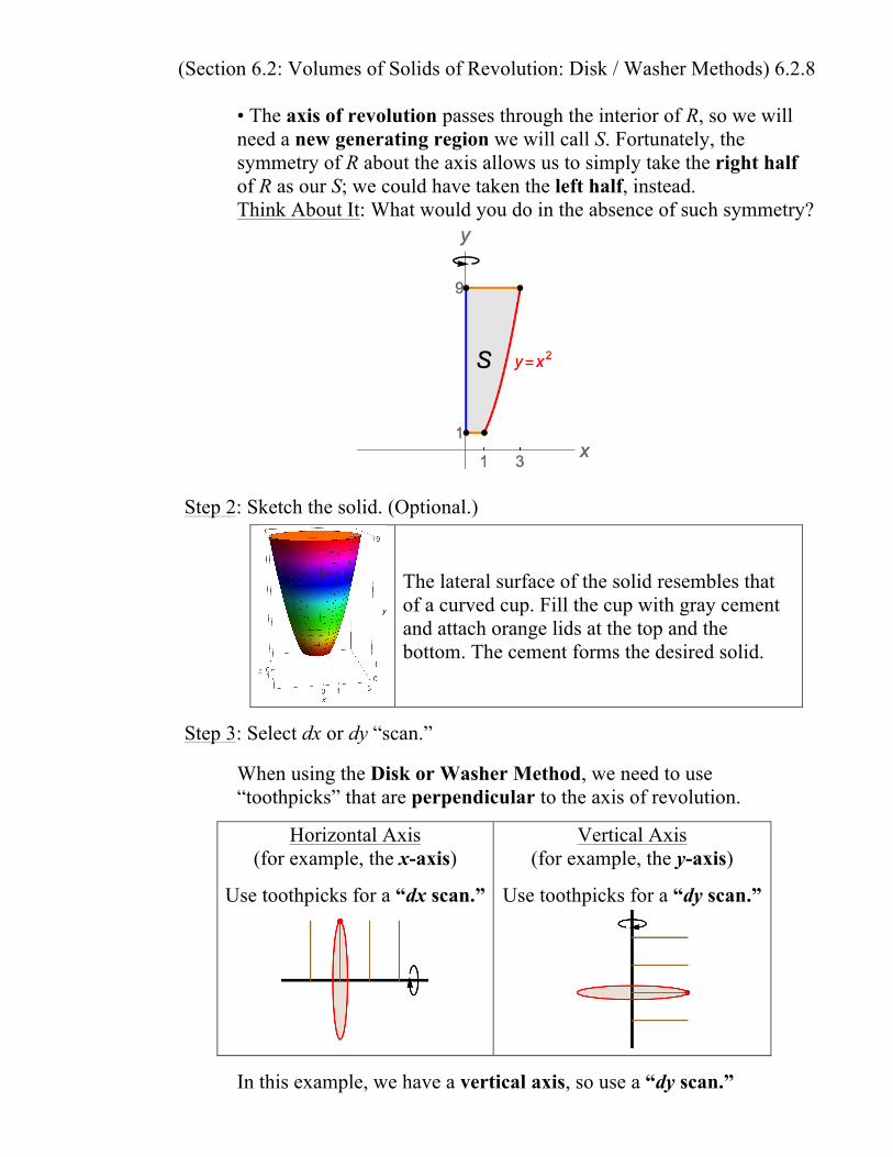
• The axis of revolution passes through the interior of R, so we will need a new generating region we will call S. Fortunately, the symmetry of R about the axis allows us to simply take the right half of R as our S; we could have taken the left half, instead. Think About It: What would you do in the absence of such symmetry?

Step 2: Sketch the solid. (Optional.)

The lateral surface of the solid resembles that of a curved cup. Fill the cup with gray cement and attach orange lids at the top and the bottom. The cement forms the desired solid.

Step 3: Select dx or dy “scan.”

When using the Disk or Washer Method, we need to use “toothpicks” that are perpendicular to the axis of revolution.

Horizontal Axis (for example, the x-axis)

Use toothpicks for a “dx scan.”

Vertical Axis (for example, the y-axis)

Use toothpicks for a “dy scan.”

In this example, we have a vertical axis, so use a “dy scan.”


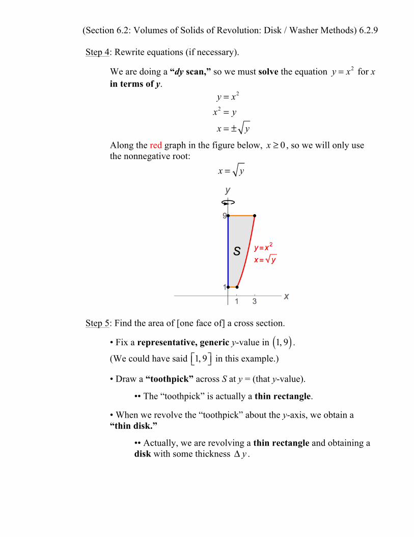
Step 4: Rewrite equations (if necessary).

We are doing a “dy scan,” so we must solve the equation y = x2 for x

in terms of y.

y = x2

x2 = y

x = ± y

Along the red graph in the figure below, x ≥ 0 , so we will only use the nonnegative root:

x = y

Step 5: Find the area of [one face of] a cross section.

• Fix a representative, generic y-value in 1, 9( ) .

(We could have said 1, 9⎡⎣ ⎤⎦ in this example.)

• Draw a “toothpick” across S at y = (that y-value).

•• The “toothpick” is actually a thin rectangle.

• When we revolve the “toothpick” about the y-axis, we obtain a “thin disk.”

•• Actually, we are revolving a thin rectangle and obtaining a disk with some thickness Δ y .


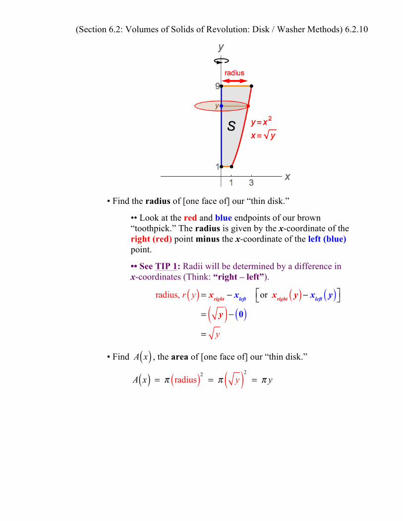
• Find the radius of [one face of] our “thin disk.”

•• Look at the red and blue endpoints of our brown “toothpick.” The radius is given by the x-coordinate of the right (red) point minus the x-coordinate of the left (blue) point.

•• See TIP 1: Radii will be determined by a difference in x-coordinates (Think: “right – left”).

radius, r y( ) = xright − xleft or xright y( )− xleft y( )⎡⎣ ⎤⎦

= y( )− 0( )= y

• Find A x( ) , the area of [one face of] our “thin disk.”

A x( ) = π radius( )2

= π y( )2= π y


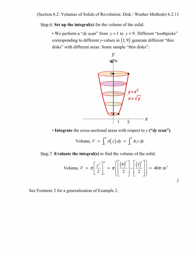
Step 6: Set up the integral(s) for the volume of the solid.

• We perform a “dy scan” from y = 1 to y = 9 . Different “toothpicks” corresponding to different y-values in 1, 9( ) generate different “thin disks” with different areas. Some sample “thin disks”:

• Integrate the cross-sectional areas with respect to y (“dy scan”).

Volume, V = A y( ) dy

1

9

∫ = π y dy1

9

∫

Step 7: Evaluate the integral(s) to find the volume of the solid.

Volume, V = π y2

2⎡

⎣⎢

⎤

⎦⎥

1

9

= π9( )2

2

⎡

⎣⎢⎢

⎤

⎦⎥⎥−

1( )2

2

⎡

⎣⎢⎢

⎤

⎦⎥⎥

⎛

⎝⎜⎜

⎞

⎠⎟⎟= 40π m3

§ See Footnote 2 for a generalization of Example 2.

Documents

SECTION 6.2: VOLUMES OF SOLIDS OF …Section 6.2: Volumes of Solids of Revolution: Disk / Washer Methods) 6.2.2 It helps that the axis of revolution does not pass through the interior