Embed Size (px)
Citation preview

Section 3.2
Asymptotic Series, Laplace’s Method,
Gamma Function, Stirling’s Formula

( ) ( )!,
2 2 ! !
NpN N
C Nw m Np N p
= =−
• the exact form of 𝑤𝑤 𝑚𝑚,𝑁𝑁 was obtained. m: position. N: total steps.
p = (N + m)/2
• The calculation is tedious and heavy.• James Stirling (Scottish mathematician, 1692-1770)
presented a way to estimate it with enough accuracy.
3.2.0 Simplify probability function by Stirling’s formula

Stirling’s formula
3
1 1 1ln !~ ln ln 22 12 360
n n n nn n
π + − + + − +
Dominant term
( )1/2!~ 2 n nn n n eπ −
3.2.0 Simplify probability function by Stirling’s formula
will be proved later

2N mp +
=( ) ( )!,
2 ! !N
Nw m Np N p
=−
3.2.0 Simplify probability function by Stirling’s formula
( ) ( )( )
2
!ln , ln2 ! !
ln ! ln ! ln ! ln 2
2 1ln ln 1 ln 1 ln 12 2 2
N
Nw m Np N p
N p N p N
N m m m m mN N N Nπ
=−
= − − − −
+ = − − + − − +
( )1
2 2 2 22, 1 1 1
N m m
m m mw m NN N N Nπ
+− − = − − +
1ln !~ ln 2 ln2
n n n n nπ + −

2N mp +
=( ) ( )!,
2 ! !N
Nw m Np N p
=−
1ln !~ ln 2 ln2
n n n n nπ + −
3.2.0 Simplify probability function by Stirling’s formula
( ) ( )( )
( ) ( ) ( ) ( )
!ln , ln2 ! !
ln ! ln ! ln ! ln 21 1 1 1ln 2 ln ln ln 2 ln ln2 2 2 21 1ln 2 ln ln ln 22 21 1 1 1ln 2 ln ln ln 2 ln ln2 2 2 2 2 2 2 21 1ln 2 ln ln2 2 2 2 2 2
N
Nw m Np N p
N p N p N
N N N N p p p p
N p N p N p N p N
N m N m N m N mN N N N
N m N m N m N m N
π π
π
π π
π
=−
= − − − −
= + + − − − − +
− − − − − − + − −
+ + + += + + − − − − +
− − − −− − − + −
( ) ( )( )
2 2 2 2
22
ln 2
1 1 1 1ln ln ln ln ln ln ln 2 ln 22 2 2 2 2 2 2 2 2 21 1 1ln ln ln ln ln ln 2 ln 22 2 4 2 4 2 2
1 / 1 /1 1 1ln ln ln ln ln 2 ln 22 2 4 2 1 / 2
1 1ln ln ln 2 ln2 2
N m N m N m N m N m N mN N N N
N m N N m m N mN N N NN m
m N m NN mN N N N Nm N
N NN N N N
π
π
π
+ + + − − −= + − − − − − −
− − −= + − − + − −
+
− −+= + − + − −
+
+= + − − ( )( ) ( )( ) ( )( )
( )( ) ( )( ) ( )( )
22
2
1 1ln 2 ln 1 / ln 1 / ln 1 /4 2 2 2 2
2 1ln ln 1 / ln 1 / ln 1 /2 2 2
N m mm N m N m N
N m mm N m N m NN
π
π
+− − − + − − +
+= − − + − − +

( )
( )
12 2 2 2
2
2
2
2
2, 1 1 1
2 1exp exp exp2 2 2
12 exp2
2 exp2
N m m
N
m m mw m NN N N N
m N m m m mN N N N
N mN N
mN N
π
π
π
π
+− −
→∞
= − − + →
+ = − − −
= −
≈ −
1lim 1x
xe
x→∞
+ =
3.2.0 Simplify probability function by Stirling’s formula
( )22, exp
2mw m N
N Nπ
≈ −

N=5 N=100
3.2.0 Simplify probability function by Stirling’s formula
( )22, exp
2mw m N
N Nπ
≈ −
( )2
2 2
,
em
NN
w m N
π
−
m m

3.2.0 Simplify probability function by Stirling’s formula
3 5
1 1 1 1ln !~ ln ln 22 12 360 1260
n n n nn n n
π + − + + − + −
In this book, via gamma function
Stirling’s formula• 2 heuristic & 8 rigorous approaches to derive
• Diverge for any value of n.
• Not a series in rigorous mathematical sense.

3.2.0 Simplify probability function by Stirling’s formula
( )1/2!
2 n n
nn n e
απ −
=
Because it is an asymptotic series.
• But ! The dominant term works!
n
5 1.0167810 1.0083750 1.00167100 1.000837
n α
( )1/2!~ 2 n nn n n eπ −

3.2.1 Examples of asymptotics
Jules Henri Poincaré introduced asymptotic expansion
in 1886. This concept enables one to
• manipulate a large class of divergent series
• obtain numerical as well as qualitative results for
many problems.

for large x.
we have a solution in the form
this divergent series is useful for numerical
calculations, and called an asymptotic series
Example -1: ODE1dy y
dx x+ =
( )2 3
1 !1 2! 3!n
ny
x x x x−
= + + + +
3.2.1 Examples of asymptotics

Example-2: regular quadratic
ε : a small constant, say ε =0.0000001.
2 1 0x xε+ − =
2 42
x ε ε− ± +=Exact solutions
1x = ±
As ε=0, we have the unperturbed solution
3.2.1 Examples of asymptotics
2 1 0x xε+ − =

converge if
2ε <
( )
( )
2 46
2 46
12 8 128
12 8 128
Ox
O
ε ε ε ε
ε ε ε ε
− + − +=
− − − + +
Series method
2 31 2 31x a a aε ε ε= ± + + + +
power series expansion around 𝑥𝑥 = ±1
The same Taylor expansions can be reproduced.
Taylor expansion of the exact solution:
3.2.1 Examples of asymptotics

ε is a small constant, say ε =0.0000001.
Example-3: singular quadratic
Exact solutions 1 1 42
x εε
− ± +=
As ε=0, we have the unperturbed solution
1x =Only one root !
3.2.1 Examples of asymptotics

Taylor expansion of the exact solution:
( )( )
2 3 4
2 3 4
1 2 5
1 1 2 5
Ox
O
ε ε ε ε
ε ε ε εε
− + − += − − + − + +
converge if
1/ 4ε <
Expansion method
210 1 2
ax a a aε εε−= + + + +
Assuming power series
Substituting into
Why? be patient
3.2.1 Examples of asymptotics

( ) ( ) ( )1 2 0 21 1 1 0 0 1 1 0 12 1 2
0
a a a a a a a a aε ε ε−− − − −+ + + − + + +
+ =
Comparing coefficients of ε of same order
ε-1 : 21 1 0a a− −+ = 1 1a− = −
Regular root
ε0 : 1 0 02 1 0a a a− + − = 0 1a = −
ε1 : 21 1 0 12 0a a a a− + + = 1 1a =
1 1x εε
= − − + +
3.2.1 Examples of asymptotics
1or 0a− =
0 1a =
1 1a = −
2
12
x ε
ε
= −
+
Singular root

balance the three terms 2 1 0x xε + − =
Rescaling method
(1) x and −1 is comparable, assuming ε x2 is smaller than other two terms.
2 1 0 1x x xε + − = ⇒ ≈
( ) ( )2~ 1 ~ 1x O x oε
3.2.1 Examples of asymptotics
Good guess
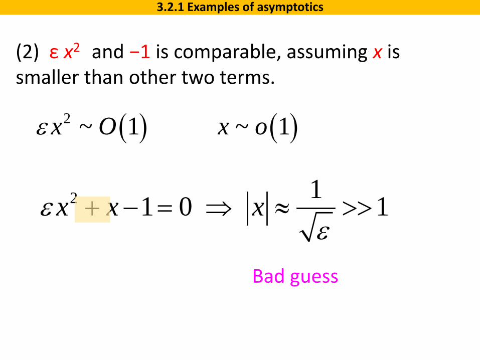
(2) ε x2 and −1 is comparable, assuming x is smaller than other two terms.
Bad guess
( ) ( )2 ~ 1 ~ 1x O x oε
2 11 0 1x x xεε
+ − = ⇒ ≈ >>
3.2.1 Examples of asymptotics

(3) ε x2 and x is comparable, assuming both terms >> 1.
( )2 ~ 1x O xε >>
Self consistent
2 11 0 1x x xεε
+ − = ⇒ ≈ >>
When ε x2 and x balance, x is very larger 𝑥𝑥~𝑂𝑂 𝜀𝜀−1
Xxε
=rescaling x, ( )with ~ 1X O
3.2.1 Examples of asymptotics
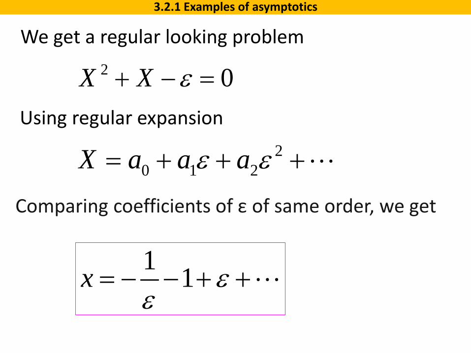
2 0X X ε+ − =
We get a regular looking problem
20 1 2X a a aε ε= + + +
1 1x εε
= − − + +
Using regular expansion
Comparing coefficients of ε of same order, we get
3.2.1 Examples of asymptotics
Example-4: Asymptotic series by parts integration3.2.1 Examples of asymptotics
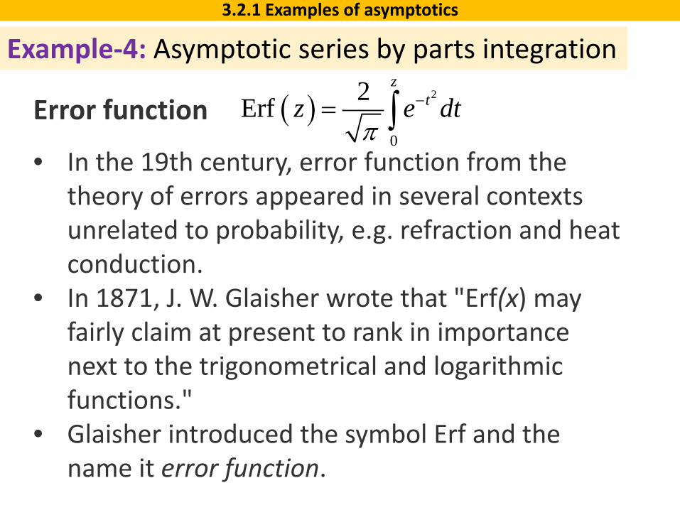
Error function
• In the 19th century, error function from the theory of errors appeared in several contexts unrelated to probability, e.g. refraction and heat conduction.
• In 1871, J. W. Glaisher wrote that "Erf(x) may fairly claim at present to rank in importance next to the trigonometrical and logarithmic functions."
• Glaisher introduced the symbol Erf and the name it error function.
( ) 2
0
2Erfz
tz e dtπ
−= ∫
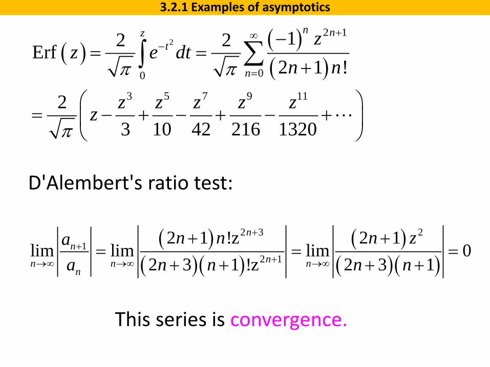
This series is convergence.
( ) ( )( )
22 1
00
3 5 7 9 11
12 2Erf2 1 !
23 10 42 216 1320
n nzt
n
zz e dt
n n
z z z z zz
π π
π
+∞−
=
−= =
+
= − + − + − +
∑∫
D'Alembert's ratio test:
( )( )( )
( )( )( )
2 3 21
2 1
2 1 !z 2 1lim lim lim 0
2 3 1 !z 2 3 1
nn
nn n nn
n n n zaa n n n n
++
+→∞ →∞ →∞
+ += = =
+ + + +
3.2.1 Examples of asymptotics

Consider an alternative form of the error function
Integrating by parts
and 3 more times
( )
( )
2 2
2
0 0
2 2Erf
21 1 Erfc
z zt t
t
z
z e dt e dt
e dt z
π π
π
∞− −
∞
∞−
= = +
= − = −
∫ ∫ ∫
∫complementary error function
( ) 2 2 22
2
Erfc2 2 22 /
t z tt
z z z
z de e ee dt dtt z tπ
∞ ∞ ∞− − −−= = − = −∫ ∫ ∫
( )( ) ( ) ( )
2 2
2 3 42 82 2 2
Erfc 1 1 3 1 3 5 1 3 5 7 10512 2 162 / 2 2 2
z t
z
z e e dtz z tz z zπ
∞− − ⋅ ⋅ ⋅ ⋅ ⋅ ⋅ = − + − + +
∫
udv uv vdu= −∫ ∫
3.2.1 Examples of asymptotics
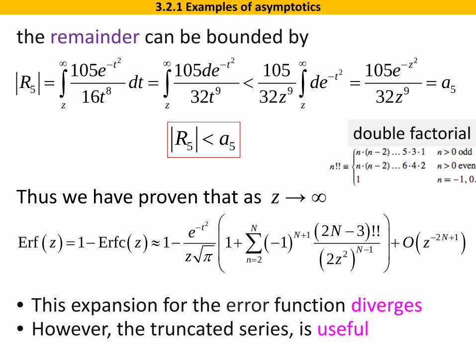
the remainder can be bounded by
5 5R a<
2 2 22
5 8 9 59 9
105 105 105 10516 32 32 32
t t zt
z z z
e de eR dt det t z z
a∞ ∞ ∞− − −
−= = < = =∫ ∫ ∫
Thus we have proven that as z → ∞
( ) ( ) ( ) ( )( )
( )2
1 2 1122
2 3 !!Erf 1 Erfc 1 1 1
2
t NN N
Nn
Nez z O zz zπ
−+ − +
−=
− = − ≈ − + − +
∑
• This expansion for the error function diverges• However, the truncated series, is useful
double factorial
3.2.1 Examples of asymptotics

This expansion has some important properties:• the leading term is roughly correct • further terms are corrections of decreasing size. This property is called asymptoticness.
z = 2.5
( )Erf 0.999593z =
3 terms give0.999599
z = 3
( )Erf 0.999978z =
3 terms give0.9999778
3 terms
z( )Erf z
1 −e−𝑧𝑧2
𝑧𝑧 𝜋𝜋1 −
12𝑧𝑧2
3.2.1 Examples of asymptotics
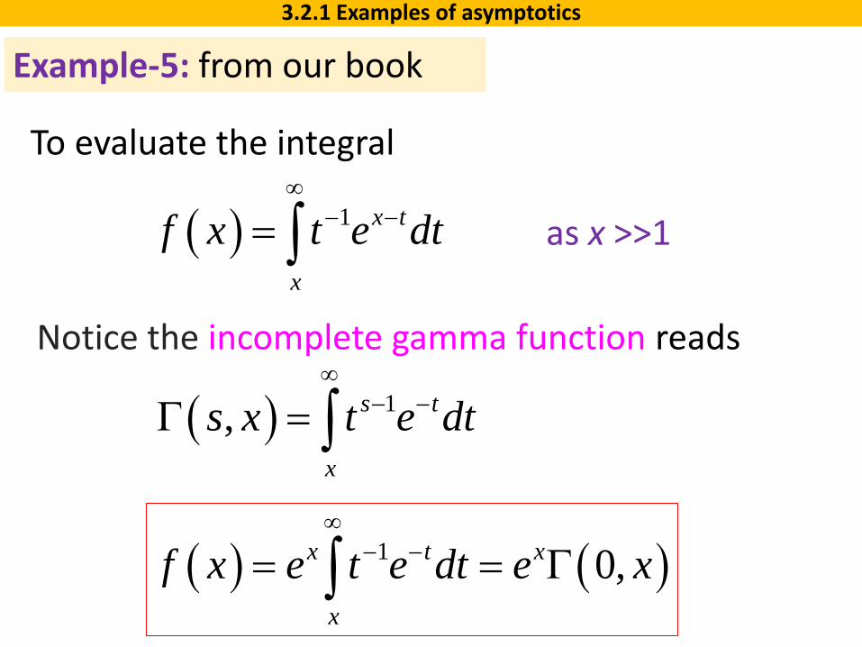
To evaluate the integral
Example-5: from our book
( ) 1 x t
x
f x t e dt∞
− −= ∫ as x >>1
Notice the incomplete gamma function reads
( ) 1, s t
x
s x t e dt∞
− −Γ = ∫
( ) ( )1 0,x t x
x
f x e t e dt e x∞
− −= = Γ∫
3.2.1 Examples of asymptotics

integration by parts, udv uv vdu= −∫ ∫( ) 1 1 1 2
2 32
|
1 1 1 2
x t x t x t x tx
x x x
x t x t
x x
f x t e dt t de t e e t dt
e t dt e t dtx x x
∞ ∞ ∞− − − − − − ∞ − −
∞ ∞− − − −
= = − = − +
= + = − +
∫ ∫ ∫
∫ ∫by successive integration by parts,
( ) ( ) ( )n nf x S x R x= +
where ( ) ( ) ( )1
2 3
1 1 !1 1 2!n
n n
nS x
x x x x
−− −= − + − +
( ) ( ) ( ) ( ) ( )11 ! 1 ! ,n nn x t xn x
R x n t e dt n e -n x∞ − + −= − = − Γ∫
3.2.1 Examples of asymptotics
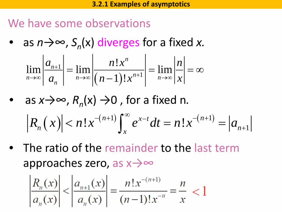
• as n→∞, Sn(x) diverges for a fixed x.
( )1
1
!lim lim lim1 !
nn
nn n nn
a n x na n x x+
+→∞ →∞ →∞= = = ∞
−
( ) ( ) ( )1 11! !n nx t
n nxR x n x e dt n x a
∞− + − +−+< = =∫
• as x→∞, Rn(x) →0 , for a fixed n.
• The ratio of the remainder to the last term approaches zero, as x→∞
3.2.1 Examples of asymptotics
We have some observations

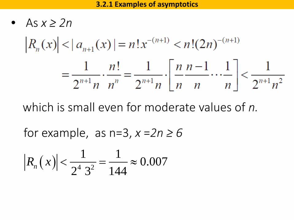
• As x ≥ 2n
which is small even for moderate values of n.
for example, as n=3, x =2n ≥ 6
( ) 4 2
1 1 0.0072 3 144nR x < = ≈
3.2.1 Examples of asymptotics
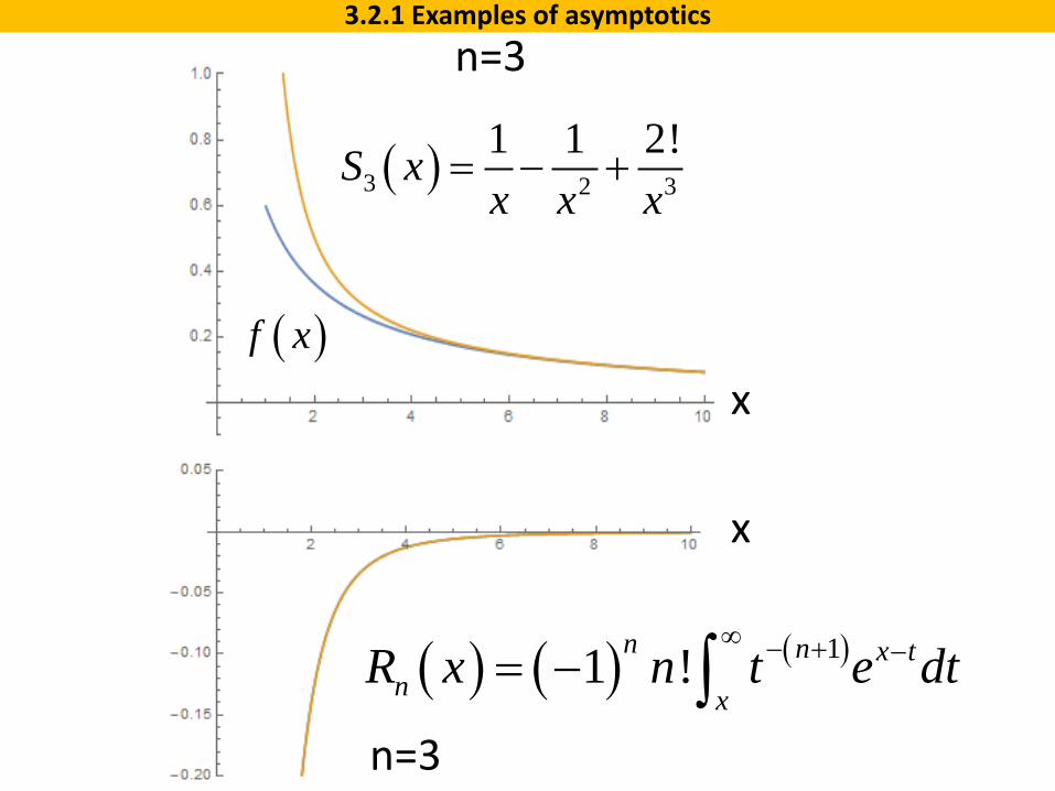
( )f x
n=3
( )3 2 3
1 1 2!S xx x x
= − +
( ) ( ) ( )11 !n n x tn x
R x n t e dt∞ − + −= − ∫
n=3
3.2.1 Examples of asymptotics
x
x
• As x ≥ 2n
which is small even for moderate values of n.
for example, as n=3, x =2n ≥ 6
( ) 4 2
1 1 0.0072 3 144nR x < = ≈
3.2.1 Examples of asymptotics

n=10 n=50
n=100
x x
x
This convergent series is less useful in practice.
3.2.1 Examples of asymptotics
( ) 2
0
2Erfz
tz e dtπ
−= ∫
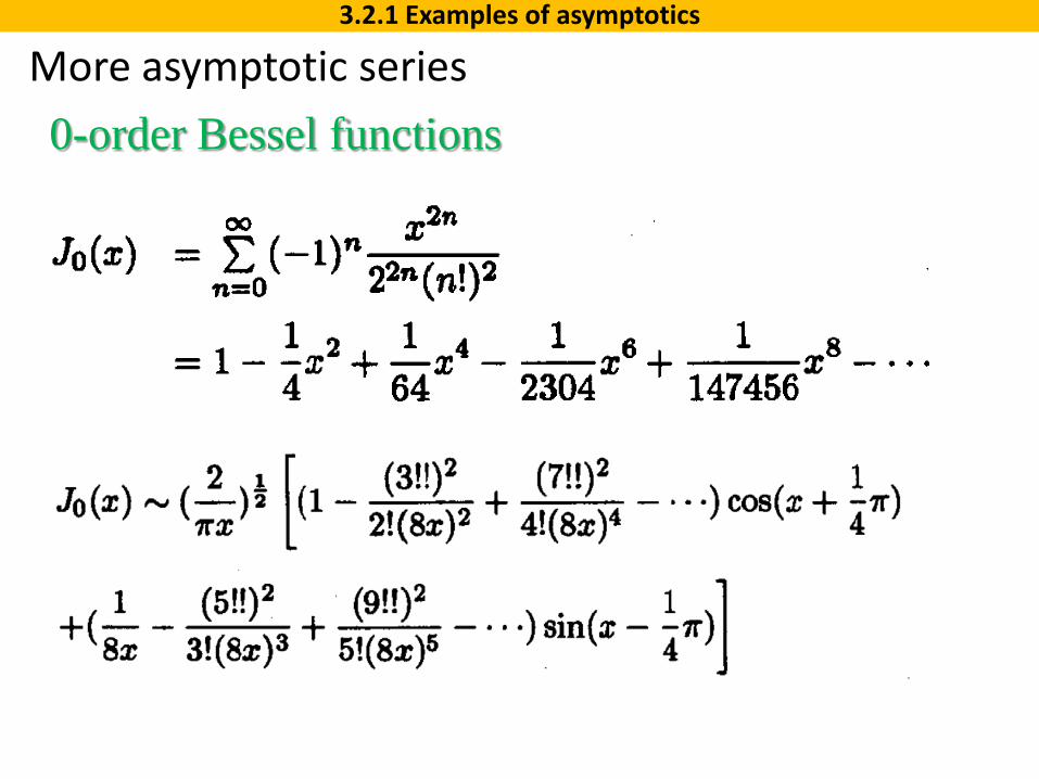
More asymptotic series0-order Bessel functions
3.2.1 Examples of asymptotics

Laplace integral
ODE
More asymptotic series3.2.1 Examples of asymptotics

Consider function f(ε) , there are three possibilities
• the speed at which f(ε) →∞ or f(ε) →0 can be expressed by comparing gauge functions.
• gauge functions may be
( ) 0, , as 0, 0f A Aε ε= ∞ → < < ∞
( ) 11/ 1 11, , , log , log log , , sin , sinh ,n n eεε ε ε ε ε ε−± ± − −
( )1/20
lim 0f
ε
εε→
=
e.g.This indicates 𝑓𝑓 𝜀𝜀 goes to 0 in a speed faster than that of 𝜀𝜀1/2
Appendix: Landau order symbols: O or o.
Appendix: Landau order symbols: O or o.
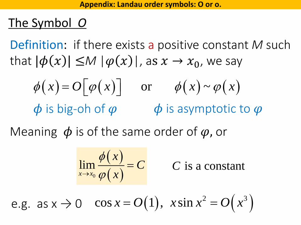
The Symbol O
Definition: if there exists a positive constant M such that |𝜙𝜙 𝑥𝑥 | ≤M |𝜑𝜑 𝑥𝑥 |, as 𝑥𝑥 → 𝑥𝑥0, we say
e.g. as x → 0
( ) ( ) ( ) ( )or ~x O x x xφ ϕ φ ϕ= 𝜙𝜙 is big-oh of 𝜑𝜑
( ) ( )2 3cos 1 , sinx O x x O x= =
( )( )0
limx x
xC
xφϕ→
=
𝜙𝜙 is asymptotic to 𝜑𝜑
Meaning 𝜙𝜙 is of the same order of 𝜑𝜑, or
is a constantC
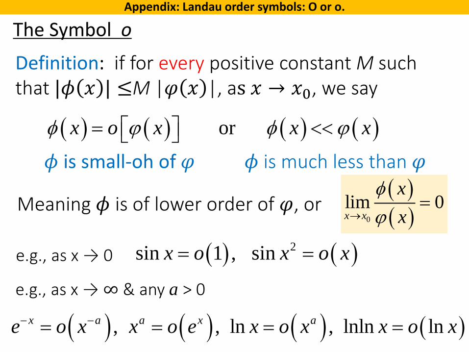
The Symbol o
( ) ( )2sin 1 , sinx o x o x= =
Definition: if for every positive constant M such that |𝜙𝜙 𝑥𝑥 | ≤M |𝜑𝜑 𝑥𝑥 |, as 𝑥𝑥 → 𝑥𝑥0, we say
e.g., as x → 0
( ) ( ) ( ) ( ) or x o x x xφ ϕ φ ϕ= <<
Meaning 𝜙𝜙 is of lower order of 𝜑𝜑, or( )( )0
lim 0x x
xx
φϕ→
=
( ) ( ) ( ) ( ), , ln , lnln lnx a a x ae o x x o e x o x x o x− −= = = =
e.g., as x → ∞ & any a > 0
𝜙𝜙 is small-oh of 𝜑𝜑 𝜙𝜙 is much less than 𝜑𝜑
Appendix: Landau order symbols: O or o.

( ) ( )!,
2 ! !N
Nw m Np N p
=−
Review
Stirling’s formula
22 exp2m
N Nπ −
3
1 1 1ln !~ ln ln 22 12 360
n n n nn n
π + − + + − +
2 1 0x xε+ − =( )
( )
2 46
2 46
12 8 128
12 8 128
Ox
O
ε ε ε ε
ε ε ε ε
− + − +=
− − − + +
( )( )
2 3 4
2 3 4
1 2 5
1 1 2 5
Ox
O
ε ε ε ε
ε ε ε εε
− + − += − − + − + +

( ) ( )( )
22 1
00
12 2Erf2 1 !
n nzt
n
zz e dt
n nπ π
+∞−
=
−= =
+∑∫
convergent series
asymptotic series( ) ( )
( ) ( )( )
( )2
1 2 1122
Erf 1 Erfc
2 3 !!1 1 1
2
t NN N
Nn
z z
Ne O zz zπ
−+ − +
−=
= −
− = − + − +
∑
• as n→∞, Sn(x) diverges for a fixed x.
• as x→∞, Rn(x) →0 , for a fixed n.
• as x→∞, |𝑅𝑅𝑛𝑛| < 𝑎𝑎𝑛𝑛
( ) ( ) ( )n nf x S x R x= +
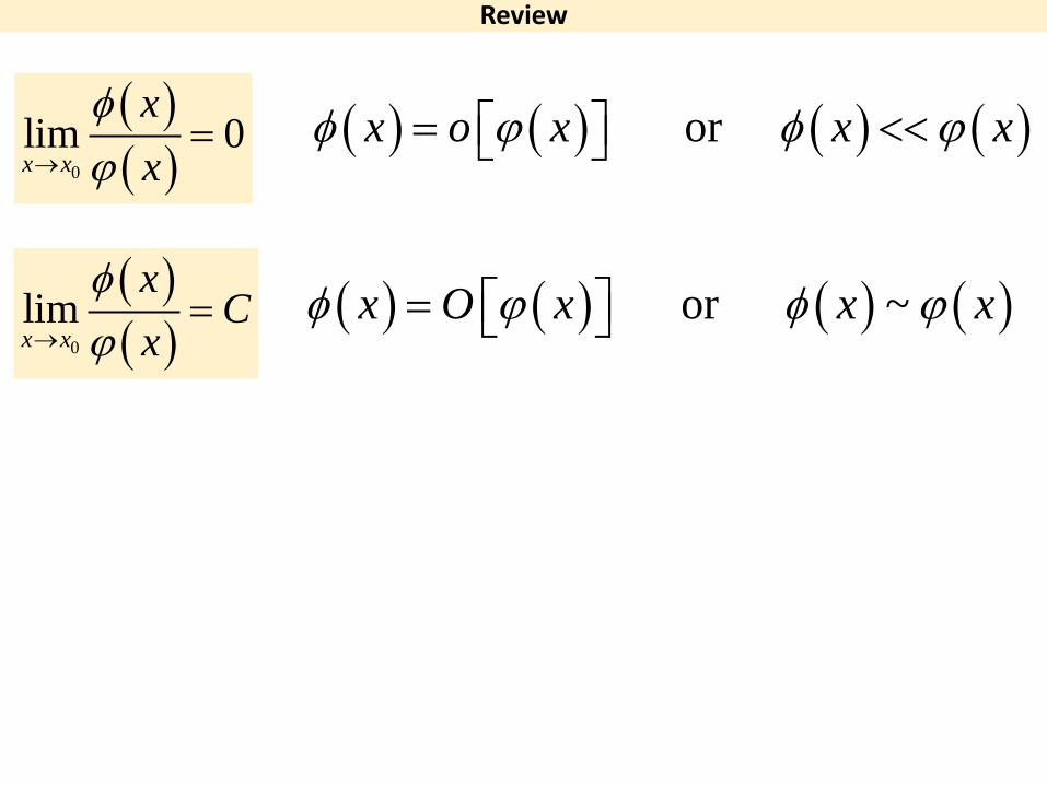
Review
Review
( ) ( ) ( ) ( ) or x o x x xφ ϕ φ ϕ= << ( )( )0
lim 0x x
xx
φϕ→
=
( ) ( ) ( ) ( )or ~x O x x xφ ϕ φ ϕ= ( )( )0
limx x
xC
xφϕ→
=

• in the example of 𝜀𝜀𝑥𝑥2 + 𝑥𝑥 − 1 = 0, we see
( )2 21 2x oε ε ε= − + +with asymptotic sequence {1, ε, ε2, …}
( )1 2 21 2x oε ε ε ε−= − − + − +with asymptotic sequence {𝜀𝜀−1, 1, 𝜀𝜀, 𝜀𝜀2,…}
• One can use a general sequence of gauge functions {φn(ε)} as asymptotic sequence as ε → 0
e.g. ( ) ( ) ( ), log , sin ...n nnnϕ ε ε ε ε−=
3.2.2 Definition asymptotic expansion
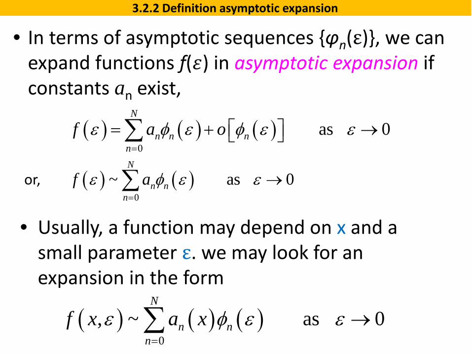
• Usually, a function may depend on x and a small parameter ε. we may look for an expansion in the form
( ) ( ) ( )0
, ~ as 0N
n nn
f x a xε φ ε ε=
→∑
• In terms of asymptotic sequences {φn(ε)}, we can expand functions f(𝜀𝜀) in asymptotic expansion if constants an exist,
( ) ( )0
~ as 0N
n nn
f aε φ ε ε=
→∑or,
( ) ( ) ( )0
as 0N
n n nn
f a oε φ ε φ ε ε=
= + → ∑
3.2.2 Definition asymptotic expansion
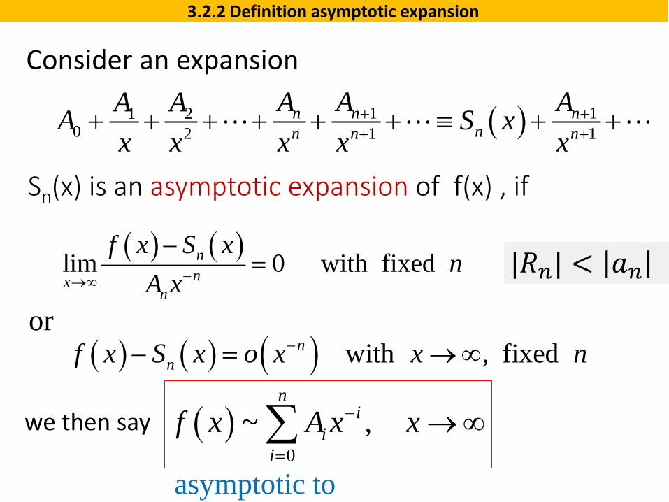
Consider an expansion
Sn(x) is an asymptotic expansion of f(x) , if
( ) ( )lim 0 with fixednnx
n
f x S xn
A x−→∞
−=
( ) ( ) ( ) with , fixednnf x S x o x x n−− = →∞
or
( )1 11 20 2 1 1
n n nnn n n
A A AA AA S xx x x x x
+ ++ ++ + + + + + ≡ + +
we then say ( )0
~ ,n
ii
if x A x x−
=
→∞∑asymptotic to
3.2.2 Definition asymptotic expansion
|𝑅𝑅𝑛𝑛| < 𝑎𝑎𝑛𝑛
( )0
~ ,n
ii
if x A x x−
=
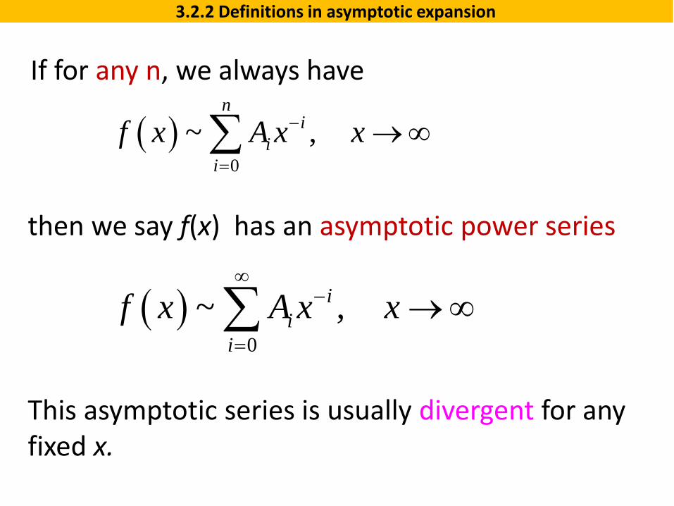
→∞∑If for any n, we always have
( )0
~ ,ii
if x A x x
∞−
=
→∞∑
then we say f(x) has an asymptotic power series
This asymptotic series is usually divergent for any fixed x.
3.2.2 Definitions in asymptotic expansion
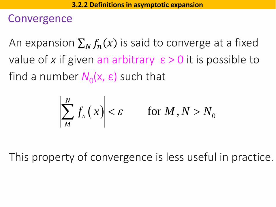
( ) 0for ,N
nM
f x M N Nε< >∑
An expansion ∑𝑁𝑁 𝑓𝑓𝑛𝑛 𝑥𝑥 is said to converge at a fixed value of x if given an arbitrary ε > 0 it is possible to find a number N0(x, ε) such that
This property of convergence is less useful in practice.
Convergence3.2.2 Definitions in asymptotic expansion

( )( )
( ) ( )
( )0 as 0
n
nn
n n
f fRf f
ε εεε
ε ε
−= → →
∑
The sum ∑𝑁𝑁 𝑓𝑓𝑛𝑛 𝜀𝜀 is said to be an asymptotic approximation to 𝑓𝑓 ε as ε →0, if for each n ≤ N
the remainder 𝑅𝑅𝑛𝑛 is smaller than the last term 𝑓𝑓𝑛𝑛.
• If the sum has this asymptotic property, one writes
( ) ( )~ as 0N
nf fε ε ε →∑
Asymptoticness3.2.2 Definitions in asymptotic expansion

More comments on convergence and divergenceLet’s look at Taylor series
• the sum converges to f(x) as n→∞. • Taylor series are de facto asymptotic expansions
( ) ( ) ( )( ) ( )( ) ( )( )2 20 0 0 0 0 0
1' ''2
f x f x f x x x f x x x o x x= + − + − + −
There are two limiting processes for an asymptotic expansion, n→∞ and ε → 0.• An asymptotic expansion provide an accurate
approximation as ε → 0 for each n• many useful expansions diverge as n→∞.
3.2.2 Definitions in asymptotic expansion

A famous example is the incomplete exponential integral
( ) ( )1
1 1 !1 1
!
nn
nn
na na n
εε
ε
++ += = + > 0
1nε =
increase as n>𝑛𝑛0
( ) ( )0 0n nR o aε =
Optimal truncation3.2.2 Definitions in asymptotic expansion
( ) ( ) ( )11
2 3
1 1 !1 1 2!~n
x tn
x
nf x t e dt
x x x x
−∞− − − −
= − + − +∫
Optimal truncation

• In practical problems, it is difficult to calculate enough terms to decide whether the asymptotic series is divergent, as opposed to mathematical asymptotic problem.
• impossible to prove that the remainder after even one or two terms is small enough.
• Luckily, one or two terms is enough for most problems encountered in applied math.
3.2.2 Definitions in asymptotic expansion

Laplace’s method :• to obtain the asymptotic expansion of certain
integrals containing a large parameter.
3.2.3 Laplace’s method
( ) ( ) ( ) 1f tF g t e dtβ
λ
α
λ λ−= >>∫idea:• the dominant contribution comes from a small
portion。
Consider

3.2.3 Laplace’s method
( ) ( )0.5 cos cos 2g t x x= + ( ) ( )2expf t x= −
( ) ( )( ) ( )20.5 cos cos 2 exp
g t f t
x x x= + −( ) ( ) ( )f tF g t e dt
βλ
α
λ −= ∫

3.2.3 Laplace’s method
Let’s stare at the integrand
( ) ( ) ( )f tF g t e dtβ
λ
α
λ −= ∫
( ) ( ) ( )200
''2
f tf t t t≈ −
a minimum at 𝑡𝑡0
( ) ( ) ( )0 2
0
0
ta t t
t
F g t e dtδ
δ
λ+
− −
−
≈ ∫
𝑡𝑡0 + 𝛿𝛿𝑡𝑡0 − 𝛿𝛿 𝑡𝑡0α β
10a =
1a =
100a =
( ) ( )20expQ t a t t = − −
( )0''2
f ta
λ−=

Taylor expansion about t0 .
Assuming
( ) ( ) ( )( ) ( )( ) ( )( )( ) ( )( )
2 20 0 0 0 0 0
20 0 0
1' ''2
1 ''2
f t f t f t t t f t t t o t t
f t f t t t
= + − + − + −
≈ + −
( ) ( )0 0' 0 '' 0f t f t= >
3.2.3 Laplace’s method
thus
( ) ( ) ( )
( ) ( ) ( ) ( )0
20 0
0
''~ exp
2
f t
f t
F g t e dt
f t t tg t e dt
βλ
α
λ
λ
λ
−
∞−
−∞
=
− −
∫
∫

( ) ( ) ( )
( ) ( ) ( ) ( )
( ) ( )
( ) ( )
( ) ( )
( )
0
0
0
20 0
0
1/2
20
0
1/2
00
''~ exp
2
2 exp''
2''
f t
f t
f t
f t
F g t e dt
f t t tg t e dt
g t e u duf t
g t ef t
βλ
α
λ
λ
λ
λ
λ
λ
πλ
−
∞−
−∞
∞−
−∞
−
=
− −
= −
=
∫
∫
∫( ) ( )0
0
''2
f tu t t= −
3.2.3 Laplace’s method
( )2exp u du π∞
−∞
− =∫
Gauss integral

3.3.4 Asymptotic Stirling series for Gamma function
( ) ( )1
0
Re 0s xs x e dx s∞
− −Γ = >∫Gamma function
( ) ( )1 1 !2
n nπ Γ = Γ = −
for s >>1, the gamma function can be reformed as
( ) ( )1 ln
0
0
s x x
sF
s e e dx
e dx
∞− −
∞−
Γ =
=
∫
∫
( ) ( )1 1, 1 lnF x s s x s x− −= − +
where
10s =
( )1 1 lns x− − 1s x−
F
x
00 1F x sx
∂= ⇒ = −
∂
0x( )ln ax o x=

3.3.4 Asymptotic Stirling series for Gamma function
The minimal 𝑥𝑥0 = 𝑠𝑠 − 1 shifts with s . Let1
xts
=−
So that the minimal point 𝑥𝑥0= 𝑠𝑠 − 1 corresponds to
t0 = 1. This leads to
( ) ( ) ( )0
1 ssFs e dx s J λ∞
−Γ = = −∫
1 1sλ = −
where
ln t− t
0 1
0t
dfdt =
= ( )0 1f t =
( ) ( )
0
f tJ e dtλλ∞
−= ∫
( ) lnf t t t= −
( )f t
t0 1t =

3.3.4 Asymptotic Stirling series for Gamma function
In order to use Laplace’s method, we modify the integrand
( ) ( ) ( ) ( )
( ) ( )
0 0
20
0 0
0
f t f t f tf t
f t w t
J e dt e dt
e e dt
λλ
λ λ
∞ ∞ − + −−
∞− −
= =
=
∫ ∫
∫where
( ) ( ) ( )20 ln 1w t f t f t t t= − = − −
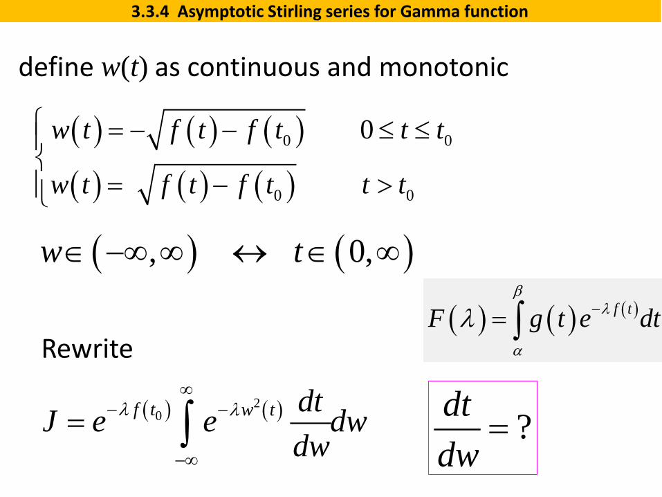
3.3.4 Asymptotic Stirling series for Gamma function
define w(t) as continuous and monotonic
( ) ( ) ( )( ) ( ) ( )
0 0
0 0
0w t f t f t t t
w t f t f t t t
= − − ≤ ≤
= − >
( ) ( ), 0,w t∈ −∞ ∞ ↔ ∈ ∞
( ) ( )20f t w t dtJ e e dw
dwλ λ
∞− −
−∞
= ∫
Rewrite
?dtdw
=
( ) ( ) ( )f tF g t e dtβ
λ
α
λ −= ∫

3.3.4 Asymptotic Stirling series for Gamma function
We now try to expand w(t) around t0=1
( )( ) ( )
( ) ( ) ( ) ( ) ( )
( ) ( ) ( )
2
2 3 4
2 3 4
1 ln
1 ln 1 1
1 11 1 1 1 1 ...2 3
1 11 1 12 3
w t t t
t t
t t t t O t
t t O t
= − −
= − − + − = − − − − − + − + −
= − − − + −
w: a small number

3.3.4 Asymptotic Stirling series for Gamma function
( ) ( )22 1 1 1 22
w t t t w= − ⇒ − =
Using the first order
0 10, 2u u= =
( ) ( ) ( ) ( )2 3 42 1 11 1 12 3
w t t t O t = − − − + −
assume an asymptotic series
20 1 21 ...t u u w u w− = + + +

3.3.4 Asymptotic Stirling series for Gamma function
( )21 21 2 1 ...t w a w a w− = + +rewrite
substituting into the Taylor expansion
( ) ( ) ( ) ( )( )2 3 32 1 11 1 12 3
w t t t o t= − − − + −
comparing term by term, we have
1 2 32 1 11 2, , , ....
3 18 27a a a= = = −
( )21 2
02 1 ... m
mm
dt d w a w a w b wdw dw
∞
=
= + + = ∑Then
0 2b =
3.3.4 Asymptotic Stirling series for Gamma function
( ) ( ) ( ) ( ) ( )2
0 0
0
f t f tw tm m
m
dtJ e e dw e b Idw
λ λλλ λ∞
− −−
=−∞
= = ∑∫
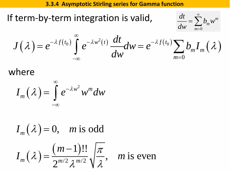
If term-by-term integration is valid,
where
( ) ( )/2 /2
1 !!, is even
2m m m
mI mπλ
λ λ−
=
( ) 0, is oddmI mλ =
0
mm
m
dt b wdw
∞
=
= ∑
( ) 2w mmI e w dwλλ
∞−
−∞
= ∫
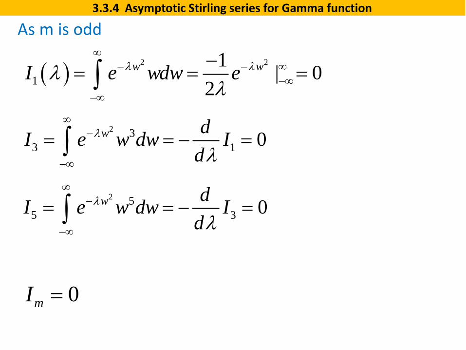
3.3.4 Asymptotic Stirling series for Gamma function
0mI =
( ) 2 2
11 | 0
2w wI e wdw eλ λλ
λ
∞− − ∞
−∞−∞
−= = =∫
2 33 1 0w dI e w dw I
dλ
λ
∞−
−∞
= = − =∫
As m is odd
2 55 3 0w dI e w dw I
dλ
λ
∞−
−∞
= = − =∫

3.3.4 Asymptotic Stirling series for Gamma function
2
0 /wI e dwλ π λ∞
−
−∞
= =∫
2 22 0
w dI e w dw Id
λ
λ
∞−
−∞
= = −∫
( )22
244 2 021w d dI e w dw I I
d dλ
λ λ
∞−
−∞
= = − = −∫
( ) ( ) ( )/2/22 0
/2 /2 /2
1 !!1 1
2
mmm
m m m m
mdI d IId d
πλ λ λ λ− −
= − = − =
As m is even

3.3.4 Asymptotic Stirling series for Gamma function
To the first order approximation
1s λ= +
( ) ( ) ( ) ( ) ( ) ( )
( )
0 0 3/20 0
0
12 / 1
f t f tm m
mJ e b I e b I O
e O
λ λ
λ
λ λ λ λ
π λ λ
− − −
=
− −
= ≈ +
= +
∑
( ) ( ) ( )1 ss s J λΓ = −( ) ( ) ( )
( ) ( ) ( )
( ) ( ) ( )
( ) ( )
1 1
1
ln ln 1
2ln 1 ln 112ln 1 1 ln ln 1
11 1 1ln 1 1 ln 22 2 1
s
s
s s J
s s e Os
s s s Os
s s s Os
λ
π λ
π λ
π
− − −
−
Γ = −
= − + + −
= − − − + + + − = − − − − + + −
0 /I π λ=0 2b =

3.3.4 Asymptotic Stirling series for Gamma function
Stirling’s approximation □
In the case of integer, i.e. s = n + 1
( )
( )1
ln ! ln 1
1 1ln ln 22 2
n n
n n n O nπ −
= Γ +
= + − + +
( )1 !n nΓ + =
( ) ( ) ( )1 1 1ln ln 1 1 ln 22 2 1
s s s s Os
π Γ = − − − − + + −