Section 1: Structures and Solid Mechanics

Boundary Element Analysis of Elastostatic Bending inRib-stiffened Orthotropic Plates

Masataka Tanaka1, Toshiro Matsumoto1 and Takahiro Nishiguchi11Department of Mechanical Systems Engineering, Shinshu University, 4-17-1

Wakasato, Nagano, 380-8553 Japan,E-mail: dtanaka@gipwc.shinshu-u.ac.jp

Keywords: Elastostatics, Computational mechanics, Plate bending, Orthotropic plate, Rib-stiffened plate, Stiffener, Boundary integral euqation, Boundary element method

Abstract. Under an accurate modeling of the rib-stiffened plates, boundary element techniquesare applied to the solution of elastostatic bending. In addition to the distributed force loads in thein-plane and out-of-plane directions on the contact line of the stiffener, distributed moment loads aretaken into account in the present theory. That is, the torsional as well as extensional rigidities, andalso beding stiffness of the stiffener are taken into consideration. A new computer code has beendeveloped, and a few examples are computed by means of the proposed solution procedure. Theresults obtained are compared with those by the conventional theory, whereby the validity of thepresent theory and the effectiveness of the solution procedure are demonstrated.

1 Introduction

This paper is concerned with a boundary element analysis of the elastostatic bending of the or-thotropic plates stiffened with straight elastic beams. Formulations of the problem can be classi-fied into the following two categories: The one is that the lateral displacement of the plate is theunknown of governing differential equation, and the other is that the interactive loads acting on thecontact line of the stiffener are treated as unknowns of the system to be solved. Hu-Hartley[1] andTanaka-Bercin[2] have investigated the problems by means of the former procedure, using interpo-lation functions of 6th-order polynominals for discretization of the contact line. On the other hand,Sapountzakis-Katsikadelis[3] and Tanaka et al.[4] have applied the latter approach based on the inte-gral equation formulation, and obtained successful results. The main advantage of the latter approachis that any type of elements can be used for numerical implementation of the formulations. Tanaka etal.[4] have presented an accurate boundary element method based on the latter approach, and showedgood numerical results of some examples. It is interesting to note that the above boundary integralequation method by the authors[4][5] introduces an accurate modeling of the rib-stiffened plates inwhich distributed moment loads are assumed to act on the contact line of the stiffener in addition tothe distributed force loads. It can be mentioned that more accurate numerical results are obtained,without use of higher-order elements for discretization of the contact line.

Timoshenko’s theory[6] is available for the stiffened isotropic plates, but it is assumed in thistheory that the neutral line of the stiffener is in the middle plane of the plate and that the cross-sectionof the beam-stiffener is doubly symmetric. In a more accurate modeling of the stiffened plate, theseassumptions should be eliminated. This paper presents an accurate modeling of the orthotropic platesstiffened by straight beams with torsional and bending rigidities. Extension is made of the proposedapproach[4][5] for the stiffened isotropic plates to the stiffened orthotropic plates. A new computercode is developed in this study, and it is applied to numerical computation of a few examples todemonstrate the validity of the proposed theory. It is revealed that there can be larger differencesbetween the present solutions and the conventional ones when the plate deforms asymmetrically.

Advances in Boundary Element Techniques V 3

Stiffener

Plate

x1

x2

x3

f^ s

1

f^ s

2f^ s

3

ms1

ms2

Stiffener

c

X

X

f^ p

1

f^ p

2f^ p

3

mp1

mp2

Plate

c

c'

X1

2

3

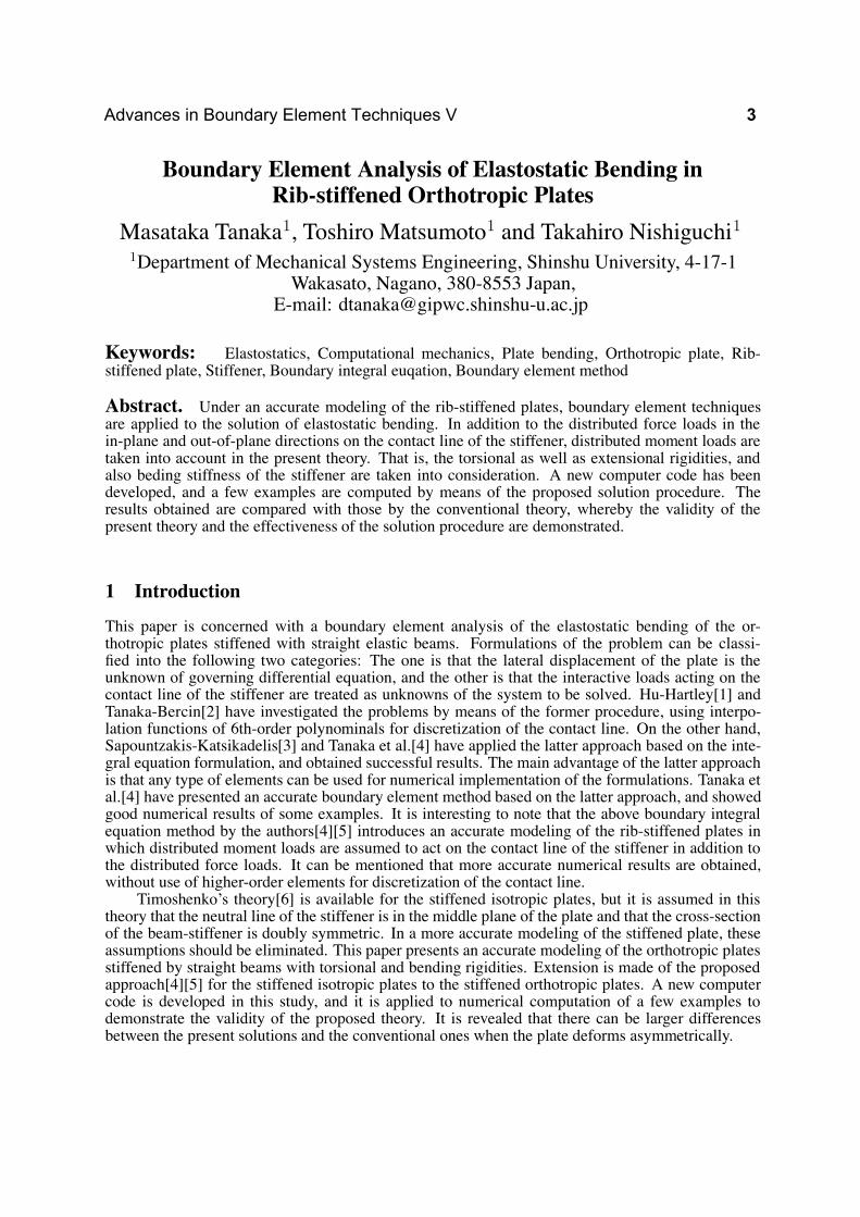
Figure 1 A model of an eccentrically stiffened plate

2 Theory

We shall consider a beam-stiffened orthotropic plate as sown in Fig. 1, where the plane X1X2 coin-cides with the middle plane of the plate. The right-hand system of coordinates is introduced, where theaxis x1 is the line connecting centroidal points of stiffener’s cross-section, and the axis x3 coincideswith the axis X3. In this paper, the formulation will be made under the following assumptions:

(i) The plate is connected with a stiffner along a straight contact line;

(ii) The plate is homogeneous and orthotropic;

(iii) The cross-section of stiffener is doubly symmetric, and the deformation due to extension, bend-ing and torsion are uncoupled.

(iv) The moment about the axis x3 normal to the plate middle plane is neglected, and the distributedmoment loads mi (i = 1, 2) along the axes x1 and x2 as well as the distributed force loadsfi

(i = 1, 2, 3) are taken into account.

Because the contact line in general does not exist in the plate middle plane, interactive forcesand moments on the contact line should be transformed into the equivalent loads acting on its normalprojection in the plate middle plane. That is, the interactive loads of the plate acting on the contactline Γc can be transformed into those on its normal projection Γ′

c in the plate middle plane as follows:

f p1 = f p

1 (1)

f p2 = f p

2 (2)

f p3 = f p

3 (3)

mp1 = mp

1 − αp3f

p2 (4)

mp2 = mp

2 + αp3f

p1 (5)

where αp3 is the coordinate X3 of the contact line, and usually αp

3 = ±hp/2 (h: plate thickness).For the interatctive forces and moments of the stiffener, we can calculate their components acting

on the neutral axis of the stiffener from the hatted components on the contact line as follows:

f s1 = 1f

s1 + 2f

s2 (6)

f s2 = −2f

s1 + 1f

s2 (7)

f r3 = f r

3 (8)

ms1 = 1m

s1 + 2m

s2 + αs

32fs1 − αs

31fs2 (9)

ms2 = −2m

s1 + 1m

s2 + αs

31fs1 + αs

32fs2 (10)

4

where (1, 2) are the X1, X2 components of the unit vector of the contact line. In addition, αs3 is the

x3 coordinate and in general αs3 = ±hs/2 (hs: stiffener’s height).

2.1 Integral equation for out-of-plane deformation of the plateThe plate is subjected to the prescribed loads, and also the distributed forces f p

i (i = 1, 2, 3) as well asmoments mp

i (i = 1, 2) from the stiffener which are all unknown. The governing differential equationof the orthotropic elastic plate can be expressed in terms of the displacement W of the plate middleplane as follows:

£W − F + εijMi,j = 0, x ∈ Ω (11)

where the differential operator £ can be expressed by

£ = D11∂4

∂x41

+ 2(D12 + 2D66)∂4

∂x21x

22

+ D22∂4

∂x42

(12)

It is interesting to note that Dij is the bending rigidities of the orthotropic plate, and F and Mi are thedistributed force and moment loads per unit area of the plate middle plane, respectively. In Eq.(11),the lower indexes i, j = 1, 2 imply the summation convention and the index following the commadenotes differentiation with respect to its coordnate. The notation εij is a permutation symbol definedby

εij =

[0 1

−1 0

](13)

Even for the bending of orthtropic plates we can develop the integral equation formulation in asimilar manner to the classical theory of isotropic plates[7]∼[10]. A regularized integral equation ofthe present orthotropic plates can be written as follows:∫

Γ

[W ∗Vn − Θ∗

nMn + M∗nΘn − V ∗

n

W − W (y)

]ds

+Nc∑

kc=1

[[M∗

nt

W − W (y)

− W ∗Mnt

]]kc

+

∫Ω

W ∗FdΩ +

∫Ω

εij∂W ∗

∂xjMidΩ = 0 (14)

where ni is the component of the unit normal vector to the plate boundary, and the summation∑

[[ ]]implies the sum over the number Nc of all the corners along the plate boundary. The asterisked func-tion W ∗ is the funamental solution of the differential operator £, and is available in the literature[11].

We also have to use an additional integral equation with respect to the derivative of deformationof the plate middle plane. Its reguralized expression can be given as follows:∫

Γ

[∂W ∗

∂yk

Vn − ∂Θ∗n

∂yk

Mn +∂M∗

n

∂yk

Θn − W,i(y)ni

−∂V ∗

n

∂yk

W − W (y) − riW,i(y)

]ds

+

Nc∑kc=1

[[∂M∗nt

∂yk

W − W (y) − riW,i(y)

− ∂W ∗

∂ykMnt

]]kc

+

∫Ω

∂W ∗

∂yk

FdΩ +

∫Ω

εij∂2W ∗

∂yk∂xj

MidΩ = 0 (15)

Advances in Boundary Element Techniques V 5

In order to solve the plate bending problem, we have to derive the boundary integral equation forthe normal derivative Θn(y) of the deformation, which can be derived from the above expression forW,i(y). Such detailed formulations can be found in the literature[5],[7]∼[10]. The domain integralincludes integration with respect to the distributed loads pre unit length of the contact line. Thedomain integral for the lateral loads can be interpreted as follows:∫

Ω

W ∗FdΩ =

∫Ω

W ∗QdΩ +

NL∑i=1

∫γi

W ∗f p3 dγi (16)

where the first term on the right-hand side is a domain integral for the given lateral load, and thesecond term is a summation of the line integrals for the number NL of all the contact lines .

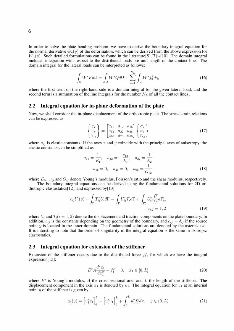
2.2 Integral equation for in-plane deformation of the plateNow, we shall consider the in-plane displacement of the orthotropic plate. The stress-strain relationscan be expressed as

εx

εy

γxy

=

[a11 a12 a16

a12 a22 a26

a16 a26 a66

]σx

σy

τxy

(17)

where aij is elastic constants. If the axes x and y coincide with the principal axes of anisotropy, theelastic constants can be simplified as

a11 =1

E1, a12 = −ν12

E1, a22 =

1

E2

a16 = 0, a26 = 0, a66 =1

G12(18)

where Ei，νij and Gij denote Young’s modulus, Poisson’s ratio and the shear modulus, respectively.The boundary integral equations can be derived using the fundamental solutions for 2D or-

thotropic elastostatics[12], and expressed by[13]

cijUi(y) +

∫Γ

T ∗ijUidΓ =

∫Γ

U∗ijTidΓ +

∫Γ′

c

U∗ij

f pi

hpdΓ′

c,

i, j = 1, 2 (19)

where Ui and Ti(i = 1, 2) denote the displacement and traction components on the plate boundary. Inaddition, cij is the constants depending on the geometry of the boundary, and cij = δij if the sourcepoint y is located in the inner domain. The fundamental solutions are denoted by the asterisk (∗).It is intersting to note that the order of singularity in the integral equation is the same in isotropicelastostatics.

2.3 Integral equation for extension of the stiffenerExtension of the stiffener occurs due to the distributed force f s

1 , for which we have the integralexpression[13]:

EsAd2u1

dx21

+ f s1 = 0, x1 ∈ [0, L] (20)

where Es is Young’s modulus, A the cross-sectional area and L the length of the stiffener. Thedisplacement component in the axis x1 is denoted by u1. The integral equation for u1 at an internalpoint y of the stiffener is given by

u1(y) =[u∗

1v1

]L

0−

[v∗

1u1

]L

0+

∫ L

0

u∗1f

s1dx, y ∈ (0, L) (21)

6

where u∗1(x1, y) is the fundamental solution of the differential equation (20), while v1 is the exten-

sional force and v∗1 is the corresponding fundamental solution. The boundary integral equations relat-

ing the displacement u1 to the other variables can be obtained by placing the source point y onto thebounday points of ther stiffener.

2.4 Integral equation for beding of the stiffener

The elastic bending of the stiffener subjected to the distributed force f and distributed moment m isgoverned by the followiing differential equation[14]:

EsId4u

dx41

− f − dm

dx1

= 0, x1 ∈ [0, L] (22)

where Es is Young’s modulus, I the moment of inertia of cross-section and u the lateral displacementof the stiffener. The lateral displacement at an internal point y is given by the following integralexpresion:

u(y) =[u∗v

]L

0−

[ϑ∗m

]L

0+

[m∗ϑ

]L

0−

[v∗u

]L

0

+

∫ L

0

(u∗f − ϑ∗m

)dx1, y ∈ (0, L) (23)

where ϑ is the slope of deflection, m the bending moment, v the shear force, and u∗ the fundamentalsolution of Eq. (22). The other asterisked functions denoted by ϑ∗, m∗ and v∗ are those derived fromthe fundamental solution u∗. The integral equation with respect to the slope of deflection is required,and it is obtained by differentiation of Eq. (23) with respect to the coordinate y. That is,

du(y)

dy=

[∂u∗

∂yv]L

0−

[∂ϑ∗

∂ym]L

0+

[∂m∗

∂yϑ]L

0−

[∂v∗

∂yu]L

0

+

∫ L

0

(∂u∗

∂yf − ∂ϑ∗

∂ym)dx1, y ∈ (0, L) (24)

The bending of the stiffener can be solved by using the above two integral equations.

2.5 Integral equation for torsion of the stiffenerThe stiffener is twisted about its axis x1 by the distributed twinting moment ms

1. The governingequation of this elastic torsion is given by[13]

GsI1d2ϕ

dx21

+ ms1 = 0, x1 ∈ [0, L] (25)

where Gs is the shear modulus, I1 the polar moment of inertia of cross-section and ϕ the twistinangle of the stiffener about the axis x1. A detailed integral equation is omitted here because of spacelimitation.

2.6 Equilibrium of forces and moments on the contact lineAt a point on the contact line, there are five components of the distributed loads from the plate side,and furthermore five components of the distributed loads from the stiffener side, totally ten compo-nents. Through equilibrium of ditributed loads on the contact line, we can reduce the number ofunknowns from ten to five. The following relations must hold on the contact line:

f pi + f s

i = 0, i = 1, 2, 3 (26)

mpi + ms

i = 0, i = 1, 2 (27)

Advances in Boundary Element Techniques V 7

2.7 Continuity of displacements and rotations on the contact lineBecause there are five components of distributed loads on the contact line, there should be five equa-tions for continuity of displacements and rotations. In this paper, we shall use three components ofthe displacement vector and two components of rotations about the axes X1 and X2. In the plate,the displacement components Ui (i = 1, 2, 3) are given in the global coordinate system through theKirchhoff-Love hypothesis [6],[15] as follows:

U1 = U1 − αp3

∂W

∂X1

(28)

U2 = U2 − αp3

∂W

∂X2

(29)

U3 = W (30)

where (U1, U2, W ) are the displacements of a point on the plate middle plane. They are related to thevariables on the plate boundary through Eqs. (14) and (19), whereas the slope of deflection can berelated on the variables on the plate boundary through Eq. (15).

Similarly, the rotations Θi (i = 1, 2) can be given by

Θ1 =∂W

∂X2

(31)

Θ2 = − ∂W

∂X1

(32)

For the slopes of deflection in the above equation, we may use Eq. (15).On the other hand, the variables of the stiffener are expressed in the local coordinate system,

and hence we have to transform the components into those of the global coordinate system. Thedisplacements of the global coordinate system ui (i = 1, 2, 3) can be expressed by

u1 = 1u1 − αs31

du3

dx1− 2u2 + αs

32ϕ (33)

u2 = 2u1 − αs32

du3

dx1+ 1u2 − αs

31ϕ (34)

u3 = u3 (35)

where ui (i = 1, 2, 3) are the displacement components on the neutral axis of the stiffener, and ϕ isthe rotation about the axis x1. All these variables can be related to those on the plate boundary andalso to the distributed laods on the contact line.

The rotations on the contact line can be expressed by

θ1 = 1ϕ + 2du3

dx1(36)

θ2 = 2ϕ − 1du3

dx1(37)

Eventually, the continuity conditions for the displacements and rotations can be expressed as

Ui − ui = 0, i = 1, 2, 3 (38)

Θi − θi = 0, i = 1, 2 (39)

We have redived the five equtions for the five unknowns on the contact line, and hence the elasticbending problem of stiffened orthotropic plates can be solved together with the boundary integralequations.

8

2.8 Conventional theory

The conventional theory of stiffened plates does not take accont of the distributed force load f2 and thetwisting moment of stiffener m1. This means that the following relations are assumed for equilibriumof distributed force and moment loads, i.e.,

f p1 + f s

1 = 0 (40)

f p3 + f s

3 = 0 (41)

mp2 + ms

2 = 0 (42)

In consistency with the above assumptions, equations with respect to U2，u2, Θ1 and θ1 are eliminatedfrom Eqs. (38) and (39). Through this treatment three equations remain for three unknown distributedloads, that is,

U1 − u1 = 0 (43)

U3 − u3 = 0 (44)

Θ2 − θ2 = 0 (45)

The theory mentioned above is equivalent to the conventional one of stiffened plates.

3 Numerical Results and Discussions

In the conventional theory f2 and m1 are neglected, and hence there would be a larger difference fromthe present theory when such components are not negligibly small. To make sure this fact numerically,we shall investiagte two typical cases of the stiffened plates.

3.1 Numerical analysis of first exampleWe now consider the stiffened square plate with an edge length a = 1.0 [m], which is subjected touniform pressure 1.0 [Pa] as shown in Fig.2. It is assumed that the material constants of the plateare as follows: E1 = 150 [GPa]，E2 = 20 [GPa]，Poisson’ ratio ν1 = 0.3，ν2 = 0.04，ν12 = 0.3and G12 = 15 [GPa]. Furthermore, the plate thickness is assumed to be h = 0.01 [m], and theboundary conditions are shown in Fig.2. Namely, the whole plate boundary is simply supported, andthe stiffener is also simply supported at its end points located on the plate boundary.

It is also assumed that the material constants of the stiffener are as follows: Young’s modulusE = 150 [GPa] and Poisson’s ratio ν = 0.3. It is intersting to note that there is no need to assumePoisson’s ratio since the torsional rigidity of the stiffener is neglected in the conventional theory. Theshape and the dimensions of the stiffener are shown in Fig. 2. The stiffener is subject to the boundaryconditions at the two end points of no bending moment and no shear force.

Boundary elements with interpolation functions of 4th-order polynominals are used for dis-cretization of the plate boundary, and the present case employs ten equal elements for an edge ofthe square plate, while the domain of the plate is divided uniformly into 100 Lagrange elements. Thecontact line is divided into five constant elements

Advances in Boundary Element Techniques V 9

Simplysupported

Simplysupported

X1

X2

Simplysupported

Simplysupported

0.01 [m]

0.1 [m]

0.01 [m]

a

a

Figure 2 A square plate with all edges simply supported and stiffened along the line X2 = 0.5

0

0.00005

0.0001

0.00015

0.0002

0.00025

0.0003

0 0.2 0.4 0.6 0.8 1

present

conventional

Def

lect

ions

X2

Figure 3 Deflections along the center line X1 = 0.5

In Fig. 3 and Fig. 4 are shown the lateral displacements along the two different lines. Table 1summarizes the results obtained for f p

2 and mp1. The numerical results obtained for this example

are almost the same as in the conventional theory. This implies that the example, in which the platedeforms symmetrically with respect to the lines X1 = 0.5 and X2 = 0.5, shows no difference betweenthe present and conventional theories, because there is no requirement for the torsional rigidity of thestiffener.

10

Table 1 Variations of f p2 and mp

1 along the contact line by the present method

X1 X2 f p2 mp

1

0.05 0.50 0.0018071 0.0136794

0.15 0.50 -0.0026444 0.0113641

0.25 0.50 0.0006218 0.0089154

0.35 0.50 -0.0004278 0.0055506

0.45 0.50 0.0000988 0.0018737

0.55 0.50 -0.0000128 -0.0019149

0.65 0.50 0.0004147 -0.0055977

0.75 0.50 -0.0001915 -0.0089661

0.85 0.50 0.0018010 -0.0114253

0.95 0.50 -0.0014670 -0.0134792

0

0.000005

0.00001

0.000015

0.00002

0.000025

0.00003

0 0.2 0.4 0.6 0.8 1

present

conventional

Def

lect

ions

X1

Figure 4 Deflections along the center line X2 = 0.5

3.2 Numerical analysis of second exampleNext, we shall consider another example of the stiffened plate which would lead to a larger differencebetween the present and conventional theories. As shown in Fig. 5, a square plate with one edgea = 1.0 [m] stiffened partly on the plate boundary is taken into consideration. It is assumed that thematerial constants of the plate and the stiffener are the same as in the previous example. The boundaryconditions of the plate are shown in the figure.

Young’s modulus of the stiffener is assumed as E = 20 [GPa], and Poisson’s ratio ν = 0.3.

Advances in Boundary Element Techniques V 11

The shape and dimensions of the stiffener are shown in Fig. 5. It is assumed that the stiffenerlocated along the boundary X1 = a is freely supported at X2 = a/2 and at the point X2 = 0 simplysupported for bending, but clamped for the other deformation.

Discretization of the plate boundary as well as the domain of the plate are the same as in theprevious example. The contact line is now divided uniformly into 5 constant elements.

Simplysupported

Simplysupported

Free Free

X1

X2

a

0.01 [m]

0.1 [m]

0.01 [m]

aa / 2

Figure 5 A square plate with two opposite edges free and the other two edges simply supported

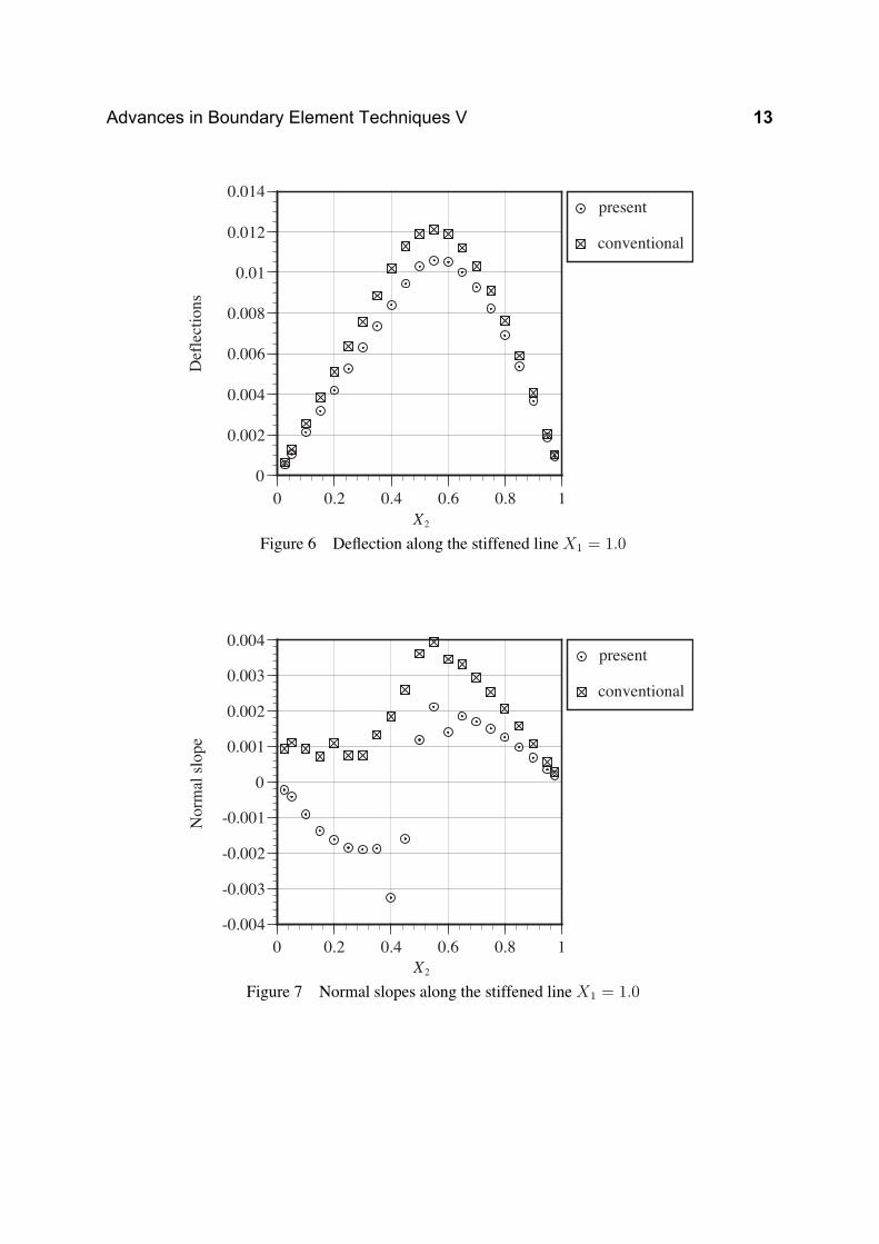
Figure 6 shows the displacement along the stiffened boundary, whereas Fig. 7 illustrates the slopeof deformation. Table 2 summarizes the results obtained for f p

2 and mp1. It can be seen that there are

larger differences between the present and convenient theories. This fact may lead us to conclude thatone must apply the present theory of the stiffened plates when a more precise analysis is required.

12

0

0.002

0.004

0.006

0.008

0.01

0.012

0.014

0 0.2 0.4 0.6 0.8 1

present

conventional

Def

lect

ions

X2

Figure 6 Deflection along the stiffened line X1 = 1.0

-0.004

-0.003

-0.002

-0.001

0

0.001

0.002

0.003

0.004

0 0.2 0.4 0.6 0.8 1

present

conventional

X2

Nor

mal

slo

pe

Figure 7 Normal slopes along the stiffened line X1 = 1.0

Advances in Boundary Element Techniques V 13

Table 2 Variations of f p2 and mp

1 along the contact line by the present method

X1 X2 f p2 mp

1

1.00 0.05 7.8771070 0.3069846

1.00 0.15 22.759608 0.3456432

1.00 0.25 1.3287552 0.4122104

1.00 0.35 -20.496443 0.3972745

1.00 0.45 6.7223875 0.3683493

4 Conclusions

In the present paper, an accurate modeling of the stiffened orthotropic plates and its numerical im-plementation have been presented. For a couple of example problems, numerical computations werecarried out and the results obtained were discussed, whereby the validity of the proposed modelingand the utility of its solution procedure have been demonstarted. The proposed theory of stiffenedorthotriopic plates would be required for more accurate numerical analysis of the plate structures.

As a future work in this direction, we may recommend further application of the proposed solutonprocedure to more complicated thin-plate structures in practical use.

References

[1] C. Hu and G.A. Hartley Engineering Analysis with Boundary Elements, 13, 229–238(1994).[2] Masa. Tanaka and A.N. Bercin Boundary Elements XIX, Brebbia, C. A. and Aliabdi, M. H.

(eds.), Computational Mechanics Publications, 203–212(1997).[3] E.J. Sapountzakis and J.T. Katsikadelis Computational Mechanics, 23, 430–439(1998).[4] Masa. Tanaka, T. Matsumoto and S. Oida Trans. JASCOME, Jour. of BEM, 24, 23–28(2000).[5] Masa. Tanaka, T. Matsumoto and S. Oida Trans. JSME, Ser.A, 66–649, 1649–1656(2000).[6] S.P. Timoshenko and S. Woinowsky-Krieger Theory of Plates and Shells, 2nd Ed., McGraw-

Hill, (1959).[7] G. Bezine and D. Gamby Recent Advances in Boundary Element Methods, Brebbia, C. A. (ed.),

Pentech Press, 327–342(1978).[8] M. Stern Progress in Boundary Element Methods 1, Brebbia, C. A. (ed.), Pentech Press, 84–

167(1981).[9] T. Matsumoto and Masa. Tanaka Singular Integrals in Boundary Element Methods, Sladek, V.

and Sladek J. (eds.), Computational Mechanics Publications, 263–297(1998).[10] T. Matsumoto, Masa. Tanaka and S. Okayama Trans. JSME, Ser.A, 64–628, 2906–2913(1998).[11] G. M. Shi and G. Bezine A General Boundary Integral Formulation for the Anisotropic

Plate Bending Problems, Laboratoire de Mecanique des Solides, Ecole Polytechnique/France,(1987).

[12] R. Yuuki Mechanics of Interfaces, Baifukan, Tokyo, (1993).[13] Masa. Tanaka, T. Matsumoto and M. Nakamura The Boundary Element Methods, Baifukan,

Tokyo, (1991).[14] M. Stern Boundary Element Methods in Structural Analysis, Beskos, D. E. (ed.), American

Society of Civil Engineers, 41–64(1989).[15] C.L. Dym and I.H. Shames Solid Mechanics – A Variational Approach, McGraw-Hill, (1973).

14

A BEM and Adjoint Variable-based approach for flaw Identification inanisotropic materials

Lucía Comino1 and Rafael Gallego2

1 Dept. Structural Mechanics, University of Granada, Politécnico de Fuentenueva, 18071 Granada,Spain, lcomino@ugr.es

2 Dept. Structural Mechanics, University of Granada, Politécnico de Fuentenueva, 18071 Granada,Spain, gallego@ugr.es

Keywords: : Identification Inverse Problem, Shape Sensitivity, Two-dimensional Anisotropic Elas-ticity, Adjoint Variable Method, Boundary Element Method (BEM)

Abstract. This communication addresses a computational strategy, based on the adjoint variable approachand BIE/BEM formulations of the direct problem, for solving identification inverse problems as flaw detection,in an anisotropic medium. The unknown shape and location of the cavities are classically sought as to achievebest fit between the measured and computed values of any physical magnitude that propagates within a bodyand that manifests on an accessible part of it. Here, the elastostatic response for a 2D body is chosen. The useof standard non-linear optimization algorithms implies the evaluation of the functional gradient with respect tothe shape parameters. A BFGS minimization algorithm has been used in conjunction with an Adjoint Variableapproach for the sensitivity computations. Boundary-only expressions of the functional derivatives have beenobtained, which are suitable for being solved with Boundary Element techniques. The good features of theproposed method are proved with several examples. Results are presented for the search of cavities of anyshape, in multi-connected homogeneous domain, but the procedure is extensible to other kinds of defects ascracks or inclusions. Also some computational issues as scaling, stopping criterion, accuracy and influence ofmeasurements errors are discussed.

Introduction

Non destructive evaluation techniques are applied to many engineering fields as quality control in industrialmanufacturing processes, sustainable maintenance of structures... in particular, flaw detection in materials isthe one treated here. This kind of problems are usually tackled as an Identification Inverse Problem (IP). Theunknown in these problems, as in shape optimization ones, is the model geometry. The solution is searchedby minimizing an integral functional, which expresses the difference between computed and measured data onpart of the external domain, e.g. in the form of least-squares distance. In order to build an efficient optimizationalgorithm, the analytical expression of the functional gradient is needed. In the present work, a formulationbased on the Adjoint Variable Method (AV) has been used, which gets a boundary-only formula for the shapesensitivity. Hence, it is suitable for using Boundary Integral Equation (BIE) techniques, which offer the minimalmodelling. This communication presents a complete strategy base in BEM for the detection in cavities planeproblems with generalized rectilinear anisotropy, in multi-connected homogeneous domain. Numerical resultsare showed.

Boundary Integral Equation. Anisotropic Fundamental Solution

The displacements of the direct problem satisfy the following BIE:

cij(y)uj(y) +∫

ΓTij(z,y)uj(z)dΓ =

∫Γ

Uij(z,y)tj(z)dΓ (1)

being Tij and Uij the anisotropic displacement and stress fundamental solutions [1] [4].

Uij(z, z′) = 2 [pj1Ai1 ln

(z1 − z′1

)+ pj2Ai2 ln

(z2 − z′2

)](2)

Tij(z, z′) = 2[

qj1Ai1

z1 − z′1(µ1n1 − n2) +

qj2Ai2

z2 − z′2(µ2n1 − n2)

](3)

Advances in Boundary Element Techniques V 15

Inverse Problem

In the present work we are dealing with Identification IP, where part of the geometry is unknown, the boundaryof the cavities Γ. Therefore, some extra information is needed in order to solve it. In this case: experimen-tal traction or displacement measurements, u and/or t, are available on an exterior boundary surface C. Thesolution of the problem is attempted by minimizing the residual between the measurements and the values com-puted in a supposed configuration uΓ and tΓ. If j is the cost function which represents the residual calculatedwith least squares distance, the functional to be minimize will be J,

J(Γ) = J(uΓ, tΓ) =∫

Cu

ju(u, u)dS +∫

Ct

jt(t, t)dS (4)

being ju = 12 |u − u|2 and jt = 1

2 |t − t|2 and Cu, Ct fixed surfaces to measure displacements and tractions.The most efficient algorithms to minimize J as BFGS, Conjugate gradients. . . [3] involve the compu-

tation of derivatives of J with respect to the unknowns of the problem. These are the design parameters of theboundary Γ which determine the position and shape of the cavity. This gradient is called shape sensitivity.

Shape Sensitivity The shape sensitivity of the functional is computed applying the Adjoint Variable approach[7]. We consider a primary problem, which has a bounded domain Ω with an external boundary δΩ, andinternal cavities with traction-free boundary Γ. The governing equations of the problem, are the ones of linearelastostatic domain, with no body forces. To study the variations of J, the material differentiation notion hasbeen introduced [8] which describes a geometrical transformation as

x ∈ Γ ⇒ x + δx = x + Θ(x)τ (5)

being Θ the transformation velocity of the boundary Γ, and τ a design time-like parameters vector. After somemanipulations, applying the Divergence Theorem, boundary conditions and tangential gradients decomposition[6] [10], a compact formula for the shape sensitivity is obtained using a local reference axis (x′

1 = n normalvector, x′

2 = t tangential vector) [11]:

∗J =

dJ

dτ=

∫Γ[σ′

22(u) : w′2,2]ΘndS (6)

with Θn the normal transformation velocity component. wi represents the displacement field of the Adjointstate governed by:

div(σ(w)) = 0 en Ω

w =−w = +j,t en Ct w = 0en δΩu/Ct

t =−t = −j,u en Cu t = 0en δΩt/Cu

Parametrization The variation of the geometry is always represented by a parametrization. Here, a conceptdeveloped by Gallego and Suárez [9] has been used. It consists in defining directly the modification field insteadof the geometry. This means applying a deformation field to some initial geometry, which is able to move ituntil any possible solution. The parametrization is defined as follows:

δxi(x) = Θipδτp (7)

Θip is the parametrization matrix and δτp is a vector with p parameters τ .A linear deformation field in 2D has been chosen, then 6 parameters are needed. The parametrization

matrix and the parameters vector are expressed in the following way [5] (with xi = xreali − xcg

i ):

Θip =[

1 0 x2 x1 x1 x2

0 1 −x1 x2 −x2 x1

](8)

16

δτp =

⎡⎢⎢⎢⎢⎢⎢⎣

δxcg1

δxcg2

δωδεm

δεl

δε12

⎤⎥⎥⎥⎥⎥⎥⎦ =

⎡⎢⎢⎢⎢⎢⎢⎣

first coordinate of the centroid of the flawsecond coordinate of the centroid of the flawrotation anglespherical strainhorizontal elongationdistortion

⎤⎥⎥⎥⎥⎥⎥⎦ (9)

Minimization Algorithm: BFGS A quasi-newton minimization algorithm has been used, the BFGS. Thevariables of the problem, parameters which define the deformation field, grouped in a vector X, are updated ineach iteration with the following scheme

Xk+1 = Xk − λkH−1k ∇fk 0 ≤ λk ≤ 1 (10)

being ∇fk the cost function gradient and Hk Hessian. The Hessian will be updated in each step with theBroyden et al (1970) approach [3].

Hk = Hk−1 +yk−1yT

k−1

yk−1Sk−1− Hk−1Sk−1ST

k−1Hk−1

STk−1Hk−1Sk−1

yk−1 = ∇f(Xk) −∇f(Xk−1) (11)

Sk−1 = Xk − Xk−1

Numerical results

Many tests have been done to prove the effectiveness of the proposed method. The results obtained in anorthotropic (birch plywood) square plate are shown. The 1m side plate, in a plane stress load state (fig.1),has been modelled with 160 isoparametric, quadratic elements. It has an elliptic cavity (discretized into 24 ele-ments, axis a=0.18334m, b=0.3m) and the initial guess to start the algorithm is a circular cavity (radius=0.08333m) far from the real position. Experimental data has been taken on the left side of the plate, displacements u2.

p1=1

p2=0

p1=0 p2=1

u1=0

p2=0

x1

x2

p1=0 u2=0

p1=1

p2=0

p1=0 p2=1

u1=0

p2=0

x1

x2

p1=0 u2=0

Figure 1: Geometry and load tests definition

Convergence Tests

Exact Measurements First, convergence of the algorithm to the solution of the problem, has been testedsupposing exact data, i.e., there is no noise in the displacement measurements. After 26 BFGS iterations, thecost functional has decreased from J0 = 0.101206 to J26 = 9.343 · 10−8 (fig.2). Another test has been donetrying to find two cavities in the plate. Although the solution is less accurate than in the previous case, thealgorithm provides a good prediction of the defect location and size (fig.2).

Effect of noise in measurements Secondly, several tests have been done introducing different noise percen-tages in the measurements. This error has been generated following a gaussian distribution. Results show avery good convergence to the real solution even with 5% error in the experimental data (fig.3).

Advances in Boundary Element Techniques V 17

BFGS iterations: exact data 1 cavity

-0.5

-0.4

-0.3

-0.2

-0.1

0

0.1

0.2

0.3

0.4

0.5

-0.5 -0.4 -0.3 -0.2 -0.1 0.0 0.1 0.2 0.3 0.4 0.5

REAL POSITION

INITIAL POSITION

LAST ITERATION (26)

BFGS: exact data - two cavities

-0.5

-0.4

-0.3

-0.2

-0.1

0

0.1

0.2

0.3

0.4

0.5

-0.5 -0.4 -0.3 -0.2 -0.1 0.0 0.1 0.2 0.3 0.4 0.5

REAL POSITION: cavity 1

REAL POSITION: cavity 2

INITIAL GUESS

parameters:1, 2, 5 and 6

parameters:1, 2, 4 and 6

parameters:1, 2, 3 and 6

parameters:1, 2, 3 and 5

parameters:1, 2, 3, 5 and 6

Figure 2: Exact data tests: one cavity (left)- two cavities (right)

BFGS iterations: 2% error in measurements

-0.5

-0.4

-0.3

-0.2

-0.1

0

0.1

0.2

0.3

0.4

0.5

-0.5 -0.4 -0.3 -0.2 -0.1 0.0 0.1 0.2 0.3 0.4 0.5

REAL POSITION

INITIAL POSITION

LAST ITERATION (26)

BFGS iterations: 5% error in measurements

-0.5

-0.4

-0.3

-0.2

-0.1

0

0.1

0.2

0.3

0.4

0.5

-0.5 -0.4 -0.3 -0.2 -0.1 0.0 0.1 0.2 0.3 0.4 0.5

REAL POSITION

INITIAL POSITION

LAST ITERATION (26)

Figure 3: Influence of 2% and 5% error in measurements

Effect of error in the material elastic constants Very often, accurate values of elastic constants are notavailable. To study its influence, several percentages of error are introduced. The following graphs show howa 5% error in the material properties, slightly increase the number of iterations needed (28 iterations) but theresult are still very good (fig.4). The decrease of the cost function along the minimization process is displayedin the next graphs (fig.5).

18

BFGS iterations: 2% error in elastic constants

-0.5

-0.4

-0.3

-0.2

-0.1

0

0.1

0.2

0.3

0.4

0.5

-0.5 -0.4 -0.3 -0.2 -0.1 0.0 0.1 0.2 0.3 0.4 0.5

REAL POSITION

INITIAL POSITION

LAST ITERATION (26)

BFGS iterations: 5% error in elastic constants

-0.5

-0.4

-0.3

-0.2

-0.1

0

0.1

0.2

0.3

0.4

0.5

-0.5 -0.4 -0.3 -0.2 -0.1 0.0 0.1 0.2 0.3 0.4 0.5

REAL POSITION

INITIAL POSITION

LAST ITERATION (28)

Figure 4: Influence of 2% and 5% noise in elastic constants

Cost Function Minimization:

error in measurements

0.E+00

5.E-04

1.E-03

2.E-03

2.E-03

3.E-03

3.E-03

4.E-03

4.E-03

5.E-03

5.E-03

0 5 10 15 20 25 30

iterations

Co

st

Fu

nc

tio

n

no error

2% error in measurements

5% error in measurements

Cost Function Minimization:

error in elastic constants

0.E+00

5.E-04

1.E-03

2.E-03

2.E-03

3.E-03

3.E-03

4.E-03

4.E-03

5.E-03

5.E-03

0 5 10 15 20 25 30

iterations

Co

st

Fu

nc

tio

n

no error

2% error in elastic constants

5% error in elastic constants

Figure 5: Cost Function evolution within the minimization process

Advances in Boundary Element Techniques V 19

Summary and conclusion

This work presents a whole strategy based on BEM, to solve Identification Inverse Problems for cavity de-tection. The developed formulation can be applied to, simple or multi-connected, 2D elastostatic domain, inanisotropic materials. The problem is tackled by minimizing a cost functional with a quasi-newton algorithm,the BFGS. This implies the previous computation of the derivatives of the functional with respect to the varia-bles of the problem. In this case, the unknowns are the design parameters which define de location and shape ofthe defect. This gradient, called shape sensitivity, has been calculated with an analytical derivation procedure,the Adjoint State approach, which allows to use Boundary Element techniques. This is very useful in problemslike the one treated, where the domain is variable, because supposes saving computational effort. Numericalresults prove the effectiveness of the proposed method.

References

[1] S.G. Lekhnitskii. Theory of Elasticity of an Anisotropic Body. Mir Publishers, Moscow, 1981.

[2] F. París y J. Cañas. Boundary Element Method. Fundamentals and Applications. Oxford University Press,1997.

[3] J.E. Dennis y R.B. Schnabel. Numerical Methods for Unconstrained Optimization and Nonlinear Equa-tions. SIAM, 1996.

[4] Paullo Sollero, Fracture Mechanics Analysis of Anisotropic Laminates by the Boundary Element Method.PhD thesis, Wessex Institute of Technology, 1994.

[5] Guillermo Rus, Métodos numéricos para la detección no destructiva de defectos PhD thesis, Grupo deMecánica de Sólidos y Estructuras, Univ. Granada 2001.

[6] M. Bonnet. Regularized BIE formulations for first and second-order shape sensitivity of elastic fields.Computers and Structures, 56, pp.799-811, 1995.

[7] M. Bonnet. BIE and material differentiation applied to the formulation of obstacle inverse problems.Engineering Analysis with BEM,ed. Elsevier, 15, pp.121-136, 1995.

[8] M. Bonnet. Sensitivity analysis for shape perturbation of cavity or internal cracks using BIE and adjointvariable approach. International Journal of Solids and Structures,ed. Pergamon, 39, pp.2365-2385, 2002.

[9] R. Gallego y J. Suarez. Numerical solution of the variation boundary integral equations for inverse prob-lems.1999

[10] H. Petryc y Z. Mroz. Time derivatives of integrals functionals defined on varying volume and surfacedomains. Arch. Mech., 38, pp.1579-95, 1986.

[11] L. Comino y R. Gallego. Shape Sensitivity of the Anisotropic Elastic Response. Proceedings of the Inter-national Conference on Boundary Element Techniques IV, 165-170, (2003).

20

On a criterion-independent tangentoperator for elastoplastic BEM analysis

L. S. Miers1, J. C. F. Telles2

Programa de Engenharia Civil – COPPE/UFRJ – Cidade Universitária – Centro de Tecnologia – Bloco I, sala I 200 – Ilha do Fundão, Rio de Janeiro / RJ – Brasil

1lsmiers@coc.ufrj.br2telles@coc.ufrj.br

Keywords: elastoplasticity, boundary elements, implicit algorithms.

Abstract. As can be verified, most formulations involving the use of the so-called consistent elastoplastic tangent operator procedure, in boundary element analysis, have been presented taking in consideration only aJ2 type yield criterion, like von Mises. The present paper aims at bringing a general consistency concept totangent operators obtained without yield criterion particularization, ready to be used in implicit schemes for elastoplastic BEM analysis. The ideas follows much of the second author’s physically nonlinear implicitBEM solution procedures introduced in the 80’s and is based on a Taylor series expansion of the true effective stress around an equivalent stress, associated to fictitious stress values corresponding to theaccumulated true stresses up to, but not including, the current increment taken to be “elastic”. To illustratethe efficiency of the technique, some comparative results using different yield criteria are presented.

Introduction

The first implementation of BEM to nonlinear analysis is due to Riccardella [1] where a pure incrementalsolution scheme was used for inviscid plasticity problems obeying the von Mises yield criterion.

As pointed out in Telles [2], until the mid eighties all the developed algorithms for BEM elastoplastic analysis were mostly based on explicit schemes, which had shown to be quite efficient untilthen. That work was the first to present implicit routines to solve elastoplastic problems by BEM and wascontinued by Telles and Carrer [3-5]. Some improvements were made after that, mainly due to the use of modified tangent operators included in the previous implicit schemes and the most implemented ones are theso-called Continuum Tangent Operator (CON) and the Consistent Tangent Operator (CTO).

Continuum implicit BEM formulations have been presented by Telles [2] and later by Jin et al. [6].It was also efficiently used in the analysis of large-strain viscoplastic problems by Mukerjee and Leu [7].The CTO was brought to the BEM context by Bonnet and Mukerjee [8] from a rate-independent plasticityFEM formulation presented by Simo and Taylor [9]. Details about the differences of CON and CTO can befound in Poon and Mukerjee [10] and in Paulino and Liu [11]. However, all the CTO-based implicit schemesfound in literature were mostly based on a J2 type yield criterion, such as von Mises’, which is not generallywell suited for all problems (e.g., soil or concrete).

The present work aims at introducing the concept of tangent operators, obtained without any kind ofyield criterion particularization, to be used in implicit schemes for elastoplastic analysis by BEM. To illustrate the efficiency of the technique, some comparative results achieved with other methods are presented in the end.

BEM Formulation for elastoplastic analysis

For the solution of general inelastic problems by the BE technique, a boundary integral equation can be obtained through weighted residual procedures or in the light of simple reciprocal statements [12]. Herein,only its final form is shown (body forces are neglected for simplicity),

)()(),()()(),()()(),()()( *** xdxxxdxuxpxdxpxuuc pjkjkijijjijjij (1)

and the derivatives of eq. (1), written for , can be combined to represent the internal stress rates in thefollowing form

Advances in Boundary Element Techniques V 21

)()()(),()()(),()()(),()( *** pklij

pklijklkijkkijkij gxdxxxdxuxpxdxpxu (2)

Equations (1) and (2) are well detailed in ref. [12].

Spatial discretization

Equation (1) leads to p

QpGuH (3) and computation of stresses at selected boundary nodes [12] and internal points (here using eq. (2)) can becarried out by

p*QuH'pG' (4)

After the application of the displacement and traction boundary conditions, eqs. (3) and (4) can bewritten as

(5) pQfyA

and

(6) p*QfyA' '

Equation (5) can then be solved for the boundary unknowns included in vector y

(7) mKyp

where m represents the elastic solution to the boundary problem. Substituting (7) into (6) and rearranging,

nS p (8) in which vector represents the elastic solution in terms of stresses. In addition: n

mA'fn

fAm

KA'QS

QAK

1

*

1

'

Constitutive equations

The incremental stress-strain relations for inviscid plasticity problems can be written in the form

klepijklij C (9)

where in eq. (9) is the fourth-order elastoplastic tangent operator that relates total strain increments with

stress increments:

epijklC

opklopmnijmnijklepijkl CaaCCC

`

1 (10)

and the meaning of every term of eq. (10) can be found in ref. [12].Introducing the fictitious “elastic” stress increment defined by

klijkleij C (11)

and the inelastic stress increment that connects with , as eij ij

klopklijopklopklopmnijmnp

ij CDCaaC`

1 (12)

equation (9) can be rewritten as eq. (13),

eopopmnijmn

eijij aaC

`

1 (13)

which shows that the true stress increments can be computed from the elastic stress in incremental form. In addition, the plastic strain increments can be calculated by the relation in eq. (14).

eopopmnijmn

pklijkl aaCC

`

1 (14)

22

and adopting the work hardening hypothesis

(15) peij

pij a

Implementation Procedures

The stress at any instant can be computed from the stress related to the last change of state and the current stress increment follows

ijbeforeijnowij (16)

The stress increment, considering the work hardening hypothesis shown in eq. (15), is defined as

(17) peklijkl

eij

pij

eijij aC

where is the equivalent plastic strain increment, which can be calculated by solving the following

general nonlinear consistency equation

pe

peijklijklee aaCe

ijijijij )()( (18)

and, in this case,

ij

e

ij

eijija

)(

where is the equivalent or effective stress considering a pure elastic stress increment.)( eijije f

Equation (18) is achieved by a Taylor Series expansion of the true equivalent stress around its value calculated at the last load step plus the pure fictitious “elastic” stress increment. Mathematically, this is shown as

pijp

ij

e

ee

eijij

eijijijij

)(

)()( (19)

Expanding the second term in the right of eq. (19) leads to

pijp

ij

klkle

pijp

ij

kl

kl

e

ee aeijij

eijij

eijijijij )(

)(

)()( (20)

Taking the non-dependence of the pure elastic stress on the plastic strain in consideration, thederivative term becomes

ijklklijpij

pkl

pij

pkl

pij

ekl

pij

kl CC (21)

Substituting eq. (21) in (20) leads to p

ijklijklee aCeijijijij )()(

(22)

Considering the hypothesis of work hardening, eq. (22) becomes eq. (18). Such an equation includes as aparticular case the consistency equation presented by Simo and Taylor [9] based on von Mises’ criterion andused in a BEM context by Mukerjee et al. [8], but is here in a general form without any restrictions about yield criterion.

The procedure to solve iteratively eq. (8) is not much different from what was presented in refs. [2-5,10,11]. The structure of the implicit algorithm is the following:

For :10 TNn1. Compute nn

2. Initialize ne

Iterative solution of 0nDS)(eee :

2.1. i = 0

2.2. Compute residual .)(e

2.3. Test if the convergence condition is satisfied: case YES, GOTO 3. 2.4. i := i + 1

3

Advances in Boundary Element Techniques V 23

2.5. Compute the local tangent operators for all nodes and determine which node is plastic or elastic.

2.6. Set up the global tangent operator.

2.7. Solve )(IDSee

2.8. Update: eee

2.9. GOTO 2.2 for new iteration 3. Update:

ppp

eDI

Results:

The results presented here are compared with the ones obtained with a well-established explicit [12] initial stress BEM technique.

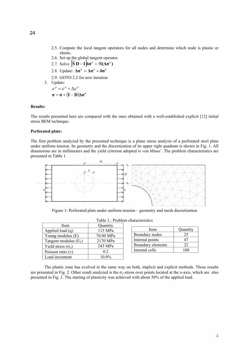
Perforated plate:

The first problem analyzed by the presented technique is a plane stress analysis of a perforated steel plateunder uniform tension. Its geometry and the discretization of its upper right quadrant is shown in Fig. 1. All dimensions are in millimeters and the yield criterion adopted is von Mises’. The problem characteristics are presented in Table 1.

q q

5

10

18

Figure 1: Perforated plate under uniform tension – geometry and mesh discretization

Table 1.: Problem characteristicsItem Quantity

Applied load (q) 115 MPa Young modulus (E) 70.00 MPa Tangent modulus (ET) 2170 MPaYield stress ( y) 243 MPa Poisson ratio ( ) 0.2Load increment 10.0%

Item QuantityBoundary nodes 25Internal points 47Boundary elements 22

Internal cells 108

The plastic zone has evolved in the same way on both, implicit and explicit methods. These results are presented in Fig. 2. Other result analyzed is the y-stress over points located at the x-axis, which are alsopresented in Fig. 2. The starting of plasticity was achieved with about 50% of the applied load.

4

24

0

5

10

15

20

25

30y/Y

Explicit BEM

Implicit BEM

0,5 0,6 0,7 0,8 0,9 1

Figure 2: Plastic deformation zones; y-stress at x-axis

Strip footing:

The last example presented is a plane strain analysis of a flexible strip footing under uniform loading. Its geometry and the discretization is in Fig. 3. All dimensions are in feet and the yield criterion adopted in this problem is Mohr-Coulomb’s. The problem characteristics can be seen in Table 2.

q

12

24

5

Figure 3: Flexible strip footing under uniform pressure

Table 2: Problem characteristicsItem Quantity

Applied load (q) 1.26 MPa Young modulus (E) 210 MPa Tangent modulus (ET) -Poisson ratio ( ) 0.3Cohesion 0.07 MPaFriction angle 20ºLoad increment 12.5%

Item QuantityBoundary nodes 25Internal points 47Boundary elements 22

Internal cells 108

x/r

The results plotted in Fig. 4 are the relation between the displacement of the node at the center of the loading and the applied load.

0

0,1

0,2

0,3

0,4

0,5

0,6

0,7

0 2 4 6 8 10 12 14 16

Implicit BEM

Explicit BEM

Elastic

ua/l

q/c’

Figure 4: Displacement of the center of the loading vs. applied load

5

Advances in Boundary Element Techniques V 25

The evolution of the plastic zone in the problem is shown in Fig. 5 for both methods. The growth ofthe plastic zone follows the same path in each one, up to the last converged solution.

Figure 5: Plastic zone evolution – (a) explicit BEM; (b) implicit BEM. (a) (b)

Conclusions

The main goal of this work is to introduce a proper criterion-independent tangent operator implicit technique for elastoplastic problems with boundary elements, generalizing what was previously presented using just aJ2-type yield criteria.

The results achieved with the multi-criteria implicit technique show its accuracy and the observedreduction in the number of iterations per load step has been over 5 times in comparison with the explicitcounterpart .

References

[1] P.C. Riccardella An implementation of the boundary integral technique for planar problems inelasticity and elastoplasticity, SM-73-10, Dept. Mech. Engng., Carnegie Mellon Univ., Pittsburg(1973).

[2] J.C.F. Telles On inelastic analysis algorithms for boundary elements, Winter Annual Meeting of the ASME, AMD Vol. 72 (T. Cruse, A. Pifko, H. Arnen, eds.), Miami, USA, 35-44 (1985).

[3] J.C.F. Telles and J.A.M. Carrer Implicit solution techniques for inelastic boundary element, 10thBEM,vol 3, 3-15 (1988).

[4] J.C.F. Telles and J.A.M. Carrer Implicit procedures for the solution of elastoplastic problems by the boundary element method, Math. Comput. Model., 15, 303-311 (1991).

[5] J.C.F. Telles and J.A.M. Carrer Static and transient dynamic nonlinear stress analysis by the boundaryelement method with implicit techniques, Engrg. Anal. Boundary Elem., 14, 65-74 (1994).

[6] H. Jin, K. Runesson, K. Matiasson Boundary element formulation in finite deformation plasticity usingimplicit integration, Comput. Struct., 31, 25-35 (1989).

[7] L.J. Leu, S. Mukherjee Sensitivity analysis of hyperelastic-viscoplastic solids undergoing largedeformations, Comput. Mech., 15, 101-116 (1994).

[8] M. Bonnet, S. Mukherjee Implicit BEM formulations for usual sensitivity problems in elastoplasticity using the consistent tangent operator concept, Int. J. Solids Struct., 33, 4461-4480 (1996).

[9] J.C. Simo, R.L. Taylor Consistent tangent operators for rate-independent elastoplasticity, Comput. Methods Appl. Mech. Engrg., 48, 101-118 (1985).

[10] H. Poon, S. Mukherjee, M. Bonnet Numerical implementation of a CTO-based implicit approach forthe BEM solution of usual and sensitivity problems in elastoplasticity, Engrg. Anal. Boundary Elem., 22, 257-269 (1998).

[11] G.H. Paulino, Y. Liu Implicit consistent and continuum tangent operators in elastoplastic boundaryelement formulations, Comput. Methods Appl. Mech. Engrg., 190, 2157-2179 (2001).

[12] J.C.F. Telles The boundary element method applied to inelastic problems, Lecture Notes in Engineering, vol.1, Springer-Verlag, Berlin Heidelberg (1983).

26

Buckling Analysis of Shear Deformable Shallow Shells

P. M. Baiz Villafranca, M. H. Aliabadi

p.m.baiz@qmul.ac.uk, m.h.aliabadi@qmul.ac.uk

Department of Engineering, Queen Mary, University of London.

Mile End Road, London E1 4NS.

Keywords: Shallow Shell, Buckling, Shear Deformable Theory.

Abstract. In the present work the linear buckling problem of elastic shallow shells by shear deformable theory is investigated. The buckling problem is presented as a standard eigenvalue problem, in order to evaluate critical loads and buckling modes. The boundary is discretized into quadratic isoparametric elements and the domain integrals are transferred into equivalent boundary integral by the use of the dual reciprocity technique. The results are compared with finite element method solutions and good agreements are obtained.

Introduction

The behaviour of curved plate structures under axial compression loads has been of major concern for engineering applications, particularly in aeronautical and aerospace structures in which the demanding design of weight critical applications usually leads to thin panels with stability problems. The buckling phenomenon has been investigated analytically and experimentally as can be found in [1,2,3,4]. Numerical solutions with Finite Element Methods (FEM) can be found in [5]. In fact, the continuous introduction of faster computers has increased the development of special computer codes as BOSOR [6] and STAGS [7] or general FEM purpose codes (ABACUS, ANSYS, IDEAS, etc.), providing designers with more tools for the modelling of stability problems in shell like structures. Other bibliographies and review papers can be found in [8]. Recently, Purbolaksono and Aliabadi [9,10] successfully applied the Boundary Element Method (BEM) to plate buckling analysis, showing the efficiency of the method for stability problems. To the best knowledge of the authors no study on the buckling analysis of shallow shells structures by the boundary element method has been reported, for classical (Kirchhoff-Love) and shear deformable (Reissner or Mindlin) theories. This paper presents a boundary element formulation for the linear elastic buckling analysis of shear deformable shallow shells. Shell buckling equations are written as a standard eigenvalue problem, which provide critical load factors and buckling modes directly as part of the solution.

Governing Integral Equations

The governing integral equations for shear deformable shallow shell bending problem can be found in detail in Dirgantara [11] and Aliabadi [12], where the formulation is formed by coupling boundary element formulations of shear deformable plate bending and two dimensional plane stress elasticity to obtain five integral equations in terms of displacement - two rotations, one out of plane displacement and two in plane displacement, which have to be solve simultaneously due to the presence of the coupling terms (curvature terms). In this work the membrane stress resultants in the domain are considered to be unknown due to external loads on the boundary. Therefore, determination of membrane stress resultants in the domain is the first step solution to the analysis of the shell buckling problem. Next, the shell buckling equations are obtained by introducing multiplication load factors of body forces ( ) in the governing integral equations for shear deformable shallow shell.

Integral Equations for In-plane Stress. The membrane stresses resultants at domain point X are written as:

Advances in Boundary Element Techniques V 27

)'(])1[(

)()()(])1([),'(

)()(),'()()(),'()'(

3

3*

*)(*

XwkvkvB

xdxnxwkvvkBxXU

xdxuxXTxdxtxXUXN i

(1)

The kernels U* and T* in eq (1) are linear combination of the first derivatives of U* and T* , and canalso be found in [11] and [12].

Integral Formulation for the Linear Buckling Problem. Appropriate forms of the linearized buckling problem can be derived transforming the shell integral equations into an equivalent shell bucklingformulation by introducing a critical load factor , resulting in a group of equations in terms of the prebuckling membrane stresses and the buckled shell displacement [9,10], as follows:

)()())(,'()()(),'(

)()())1((),'(

)()(1

2)()(

2

1),'(

)()(),'()()(),'()'()'(

,,3*33

*3

3*3

,,,*3

**

XdXwNXxWXdXqXxW

XdXwkvkvBkXxW

XdXuv

vXuXu

vBkXxW

xdxpxxWxdxwxxPxwxc

ii

i

i

jijjijjij

(2)

Where (N w3, ), (X) is a body term due to the large deflection of w3 (X). The terms cij(x ) are equal to 0.5 ij

when x is located on a smooth boundary, q3 represent transversal body force, usually set to zero in buckling problems. It is important to notice that because of the presence of the curvature terms in eq (2), this equation has to be solved simultaneously with:

)()(),'(

)()())1([),'(

)()()())1([),'(

)()(),'()'()'(

)(*

,3*

3*

)*(

xdxtxxU

XdXwkvvkBXxU

xdxnxwkvvkBxxU

xdxuxxTxuxc

i

i

(3)

The deflection equation w3 at the domain points X is required as the additional equation to arrange aneigenvalue equation, as follows:

)()())(,'()()(),'(

)()())1((),'(

)()(1

2)()(

2

1),'(

)()(),'()()(),'()'(

,,3*

333*

33

3*

33

,,,*

33

*3

*33

XdXwNXXWXdXqXXW

XdXwkvkvBkXXW

XdXuv

vXuXu

vBkXXW

xdxwxXPxdxpxXWXw jjjj

(4)

28

To arrange an eigenvalue equation, the derivatives w3, (X) and w3, (X) have to be expressed in terms ofw3(X) by making use of a radial basis function.

Numerical Examples

A computer program based on the numerical procedure described in the previous section was employed to shows the features of the developed method.

Rectangular Cylindrical Shell under Uniform Axial Compression. A rectangular cylindrical shallow shell was subjected to uniform axial compression. Two sets of boundary conditions were used: simplesupported edges (w3 = 0) and clamped edges (wi = 0). The shell has an aspect ratio a/b = 2 and width b = 2in,Young's modulus E = 1.05x107psi and Poisson ratio v = 0.33. Results are compared with Finite Elementssolutions. Buckling coefficients (K=Nc·12(1-v²)·b²/( ²·E ·t²) for different curvature parameters (Z=b²·(1-v²)0.5/(r·t))are shown in Fig.1. Buckling modes for a specific curvature parameter (Z) and different boundary conditionsare shown in Fig.2.

Conclusions

The presented Boundary Element formulation for the solution of buckling problems of Elastic ShearDeformable Shallow Shells under axial compression load shows good agreement with finite element results for the range of validity of the formulation.

1

10

100

1 10

Z

K

100

FEM - Simple Supported

BEM - Simple Supported

FEM - Clamped

BEM - Clamped

Nc

Nc

a

b

rt

Figure 1: Buckling Coefficients for Simple Supported and Clamped Rectangular Shallow Shells

Advances in Boundary Element Techniques V 29

Figure 2: Buckling Modes for Rectangular Cylindrical Shallow Shells with different Boundary Conditions.

Acknowledgement

This work was supported by Queen Mary, University of London Research Studentship. The authors wouldlike to thank Drs. Tatacipta Dirgantara, Judha Purbolaksono and Pihua Wen for fruitful discussions.

References

[1] S. Timoshenko, J. M. Gere, Theory of Elastic Stability, second edition, McGraw-Hill, New York (1961). [2] D. O. Brush, B. O. Almorth, Buckling of Bars, Plates and Shells, McGraw-Hill, New York (1975). [3] G. Gerard, H. Becker, Handbook of Structural Stability Part III - Buckling of Curved Plates and Shells, NACA TN 3783, Washington (1957).[4] W.T. Koiter, On the Stability of Elastic Equilibrium, Delft: Doctoral Thesis, (1945). English Translation:AFFDL-TR-70 25, (1970).[5] D. Bushnell, Static Collapse, A Survey of methods and modes of behaviour, Finite Elements in Analysisand Design, v1, n2, pp 165-205 (1985).[6] D. Bushnell, BOSOR5, Program for buckling of elastic-plastic complex shells of revolution including large deflections and creep. Computers & Structures, v6, pp 221-239 (1976).[7] C.C. Rankin, F.A. Brogan, W.A. Loden, H.D. Cabiness, STAGS Users Manual, version 3.0, LockheedMartin Missiles & Space Co., Inc., Advanced Technology Center, Report LMSC P032594, (1999).[8] N.F. Knight, J.H. Starnes, Developments in Cylindrical Shell Stability Analysis. Proceedings of the 38th

AIAA/ASME/ASC/AHS/ASCE Structures, Structural Dinamics, and Materials Conference, Kissimmee,Florida, pp 1933-1947 (1997). Also AIAA paper No. AIAA-97-1076. [9] J. Purbolaksono, M.H. Aliabadi, Buckling Analysis of Shear Deformable Plates by the Boundary Element Method, submitted for publication. [10] J. Purbolaksono, Buckling and Large Deformation Analysis of Cracked Plates by the Boundary ElementMethod, PhD Thesis, Department of Engineering, Queen Mary University of London (2003).[11] Dirgantara, T., Boundary Element Analysis of Crack in Shear Deformable Plates and Shells, PhDThesis, Department of Engineering, Queen Mary University of London (2000).[12] M.H. Aliabadi, The Boundary Element Method, vol II: Applications to Solid and Structures, Wiley,Chichester (2002).

30

Localized Boundary-Domain Integro-Differential Formulation forPhysically Nonlinear Elasticity of Inhomogeneous Body

S.E. MikhailovDiv. of Mathematics, Glasgow Caledonian University,

Glasgow, G4 0BA, UK, s.mikhailov@gcal.ac.uk

Keywords: Non-linear Elasticity, Variable Coefficients, Direct Formulation, Integro-Differential Equation,Localization, Mesh-based Discretization, Mesh-less Discretization

Abstract. A static mixed boundary value problem of physically nonlinear elasticity for a continu-ously inhomogeneous body is considered. Using the two-operator Green-Betti formula and the funda-mental solution of an auxiliary linear operator, a non-standard boundary-domain integro-differentialformulation of the problem is presented, with respect to the displacements and their gradients. Usinga cut-off function approach, the corresponding localized parametrix is constructed to reduce the non-linear boundary value problem to a nonlinear localized boundary-domain integro-differential equation.Algorithms of mesh-based and mesh-less discretizations are presented resulting in sparsely populatedsystems of nonlinear algebraic equations.

Introduction

Application of the Boundary Integral Equation (BIE) method (boundary element method, elasticpotential method) to linear elasticity problems for homogeneous bodies has been intensively developedover recent decades. Using fundamental solutions of auxiliary linear elastic problems (with the initialelastic coefficients), the non-linearly elastic or elasto-plastic problems for homogeneous material alsocan be reduced to non-linear boundary-domain integral equations with hyper-singular integrals, see e.g.[1–4]. However, the fundamental solution is usually highly non-local, which leads after discretization toa system of algebraic equations with a dense matrix. Moreover, the fundamental solution is generallynot available in an explicit form if the coefficients of the auxiliary problem vary in space, i.e. if thematerial is inhomogeneous (functionally graded).

To prevent such difficulties, some parametrices localized by cut-off function multiplication were con-structed and implemented in [5] for linear scalar (heat transfer) equation in inhomogeneous medium.This reduced the linear Boundary Value Problem (BVP) with variable coefficient to a linear LocalizedBoundary-Domain Integral or Integro-Differential Equation (LBDIE or LBDIDE), which leaded aftera mesh-based or mesh-less discretization to a linear algebraic system with a sparse matrix. Somenumerical implementations of the linear LBDIE were presented in [6]. Extending this approach, themixed BVP for a second order scalar nonlinear (quasi-linear) elliptic PDE with the variable coefficientdependent on the unknown solution was reduced in [7] to quasi-linear LBDIDEs. In [8], some quasi-linear two-operator LBDIDEs were obtained for the case when the variable coefficient depends also onthe BVP solution gradient. Another approach based on local parametrices that are Green functions foran auxiliary problem on local spherical domains, was used in [9] to reduce a linear elasticity problemfor a body with a special inhomogeneity, to a local boundary-domain integral equation.

In this paper, we extend the approach of [5, 8] to the mixed BVP for the system of quasi-linearpartial differential equations of physically nonlinear elasticity (with small deformation gradients) forcontinuously inhomogeneous body. First, we reduce the BVP to a direct two-operator nonlinearBDIDE of the second kind. The equation includes at most first derivatives of the unknown solution,weakly singular integrals over the domain and at most Cauchy-type singular integrals over the bound-ary. Then we present a localized version of the BDIDE and describe its mesh-based and mesh-lessdiscretizations.

Advances in Boundary Element Techniques V 31

Nonlinear Elasticity Problem, Two-operator Green-Betti Identity and BDIDE

Let us consider a mixed boundary–value problem of physically nonlinear elasticity for a boundedinhomogeneous body Ω ∈ IRn, where n = 2 or n = 3,

[Lik(u)uk](x) :=∂

∂xj

[aijkl(∇u(x), u(x), x)

∂uk(x)∂xl

]= fi(x), x ∈ Ω, (1)

ui(x) = ui(x), x ∈ ∂DΩ, (2)

[Tik(u)uk](x) := aijkl(∇u(x), u(x), x)∂uk(x)

∂xlnj(x) = ti(x), x ∈ ∂NΩ. (3)

Here u(x) = ui(x) is the unknown displacement vector; the tensor aijkl(∇u, u, x) is a known functionof u(x) and its gradient ∇u(x) = ui,j , such that aijkl = ajikl = aijlk = aklij ; fi(x) is a known volumeforce vector (taken with the opposite sign); ni(x) is an outward normal vector to the boundary ∂Ω;[T (u)u](x) = [Tik(u)uk](x) is the traction vector at a boundary point x, while T (u) = Tik(u) is thetraction differential operator; u(x) and t(x) are known displacements and tractions on the parts ∂DΩand ∂NΩ of the boundary, respectively. Summation in repeated indices is supposed from 1 to n unlessstated otherwise.

Let us fix a point y and consider the following auxiliary differential operators of the linear elasticitywith constant (frozen) coefficients,

[L(y)ik (u)vk](x) :=

∂

∂xj

[aijkl(∇u(y), u(y), y)

∂vk(x)∂xl

], [T (y)

ik (u)vk](x) := aijkl(∇u(y), u(y), y)∂vk(x)

∂xlnj(x).

Integrating by parts, we have the first Green identities for the differential operators[L(u)u](x) = [Lik(u)uk](x) and [L(y)(u)v](x) = [L(y)

ik (u)vk](x),∫Ω

vi(x)[Lik(u)uk](x)dΩ(x) =∫∂Ω

vi(x)[Tik(u)uk](x)dΓ(x) −∫

Ω

∂vi(x)∂xj

aijkl(∇u(x), u(x), x)∂uk(x)

∂xldΩ(x),∫

Ωui(x)[L(y)

ik (u)vk](x)dΩ(x) =∫∂Ω

ui(x)[T (y)ik (u)vk](x)dΓ(x) −

∫Ω

∂ui(x)∂xj

aijkl(∇u(y), u(y), y)∂vk(x)

∂xldΩ(x),

where u(x) and v(x) are arbitrary vector-functions for that the operators and integrals in the above ex-pressions have sense. Subtracting the identities from each other and taking into account the symmetryof the tensor aijkl, we derive the two-operator second Green-Betti identity,∫

Ω

u(x)[L(y)(u)v](x) − v(x)[L(u)u](x)

dΩ(x) =∫

∂Ω

u(x)[T (y)(u)v](x) − v(x)[T (u)u](x)

dΓ(x) +

∫Ω[∇v(x)]a(u; x, y)∇u(x)dΩ(x), (4)

a(u; x, y) = aijkl(u;x, y) := [aijkl(∇u(x), u(x), x) − aijkl(∇u(y), u(y), y)].

Note that if L(u) = L(y)(u), i.e. L(u) is a linear operator with constant coefficients, then the lastdomain integral disappears in eq (4), which thus degenerates into the classical second Green-Bettiidentity.

For a fixed u and y, let F (y)(u;x, y) = F(y)km(u(y),∇u(y), x, y) be a fundamental solution for the

linear differential operator [L(y)ik (u)vk](x) with constant coefficients, i.e.,

[L(y)ik (u)F (y)

km(u; ·, y)](x) := aijkl(∇u(y), u(y), y)∂2F

(y)km(u(y),∇u(y), x, y)

∂xj∂xl= δimδ(x − y),

32

where δim is the Kronecker symbol and δ(x − y) is the Dirac delta-function. Note that generallyF (y)(u;x, y) is not a parametrix for the original operator L(u) if the tensor a depends on ∇u.

If the material is isotropic, then

aijkl(∇u(y), u(y), y) = λ(∇u(y), u(y), y)δijδkl + µ(∇u(y), u(y), y)(δikδjl + δilδjk), (5)

µ(∇u(y), u(y), y) > C > 0, λ(∇u(y), u(y), y) +23µ(∇u(y), u(y), y) > C > 0.

In this case, F(y)im (u;x, y) is the Kelvin-Somigliana solution,

F(y)im (u;x, y) =

−14π

−δim ln r − r,ir,m

λ(∇u(y), u(y), y) + 2µ(∇u(y), u(y), y)+

−δim ln r + r,ir,m

µ(∇u(y), u(y), y)

(6)

for the plane strain state; for the plane stress, λ in (5) and (6) should be replaced by λ∗ = 2λµ/(λ+2µ).In the 3D case,

F(y)im (u;x, y) =

−18πr

δim − r,ir,m

λ(∇u(y), u(y), y) + 2µ(∇u(y), u(y), y)+

δim + r,ir,m

µ(∇u(y), u(y), y)

(7)

Here r :=√

(xi − yi)(xi − yi), r,i := ∂r/∂xi = (xi−yi)/r. For anisotropic material, the fundamentalsolution can be written down in an analytical form for arbitrary anisotropy in the 2D case and forsome particular anisotropy in the 3D case; otherwise, it can be expressed as a linear integral over acircle [10–12].

Assuming u(x) is a solution of nonlinear system (1) and using the fundamental solution F (y)(u;x, y)as v(x) in the Green identity (4), we obtain the following non-linear two-operator third Green identity,

c(y)u(y) −∫

∂Ωu(x)[T (y)F (y)(u; ·, y)](x)dΓ(x) +

∫∂Ω

F (y)(u;x, y)[T (u)u](x)dΓ(x)−∫Ω[∇(x)F (y)(u;x, y)]a(u; x, y)∇u(x)dΩ(x) =

∫Ω

F (y)(u;x, y)f(x)dΩ(x), (8)

where cim(y) = δim if y ∈ Ω; cim(y) = 0 if y /∈ Ω; cim(y) = 12δim if y is a smooth point of the boundary

∂Ω; and cim(y) = cim(a(y), α(y)) is a function of the anisotropy tensor a(y) and the interior spaceangle α(y) at a corner point y of the boundary ∂Ω.

Substituting boundary conditions (2), (3) into eq (8) and using it at y ∈ Ω, we arrive at a (united)nonlinear two-operator BDIDE for u(x) at x ∈ Ω

c(y)u(y) −∫

∂NΩu(x)[T (y)(u)F (y)(u; ·, y)](x)dΓ(x) +

∫∂DΩ

F (y)(u;x, y)[T (u)u](x)dΓ(x)−∫Ω[∇(x)F (y)(u;x, y)]a(u;x, y)∇u(x)dΩ(x) = F(y), y ∈ Ω, (9)

F(y) :=∫

∂DΩu(x)[T (y)(u)F (y)(u; ·, y)](x)dΓ(x) −

∫∂NΩ

F (y)(u;x, y)t(x)dΓ(x)+∫Ω

F (y)(u;x, y)f(x)dΩ(x).

BDIDE (9) is the second kind equation, which includes at most the first derivatives of the unknownsolution u(x), both directly in the domain integral term in the left hand side and through the coefficienta(∇u, u, ·) in the operators T (u), T (y)(u) and the functions F (y)(u;x, y) and a(u; x, y). The function[∇(x)F (y)(u;x, y)] is at most weakly singular in Ω, and taking into account that a(u;x, y) → 0 asx → y, we obtain that the domain integral is a smoothing operator with respect to u, for (sufficiently)smooth functions a and u. The boundary integrals have at most the Cauchy-type singularity.

Some other (e.g. segregated) BDIDEs can be obtained if one substitutes u(x) for u(x) also in theout-of-integral term of (9) at y ∈ ∂DΩ, considers the unknown boundary displacements u on ∂NΩ

Advances in Boundary Element Techniques V 33

and/or tractions T (u)u on ∂DΩ as new variables formally segregated from u in Ω, or applies theboundary traction operator to (9).

BDIDE (9) can be reduced after some discretization to a system of nonlinear algebraic equation andsolved numerically. The system will include unknowns not only on the boundary but also at internalpoints. Moreover, since the fundamental solutions, c.f. (6), (7), are highly non-local, the matrix ofthe system will be fully populated and this makes its numerical solution more expensive. To avoidthis difficulty, we present below some ideas of constructing localized parametrices and consequentlyLocalized BDIDEs (LBDIDEs).

Localized Parametrix and LBDIDE

Let χ(x, y) be a cut-off function, such that χ(y, y) = 1 and χ(x, y) = 0 at x not belonging to closure ofan open localization domain ω(y) (a vicinity of y), see Fig.1, and let P

(y)ω (u;x, y) = χ(x, y)F (y)(u;x, y).

The simplest example is

χ(x, y) =

1, x ∈ ω0, x /∈ ω

⇒ P (y)ω (u;x, y) =

F (y)(u;x, y), x ∈ ω(y)0, x /∈ ω(y)

(10)

Other examples of the cut-off functions having different smoothness are presented in [5, 6] for someshapes of ω.

Then P(y)ω (u;x, y) is a localized parametrix of the linear operator L(y), i.e.,

L(y)ik (u)P (y)

kmω(u;x, y) = δimδ(x − y) + R(y)imω(u;x, y),

where the remainder

R(y)imω = −L

(y)ik ((1 − χ)F (y)

km) = aijkl(∇u(y), u(y), y)

[F

(y)km

∂2χ

∂xj∂xl+

∂F(y)km

∂xj

∂χ

∂xl+

∂F(y)km

∂xl

∂χ

∂xj

]

is at most weakly singular at x = y, at least if χ is smooth enough on ω(y). The parametrix P(y)ω (u;x, y)

has the same singularity as F (y)(x, y) at x = y. Both P(y)ω (u;x, y) and R

(y)ω (u; x, y) are localized (non-

zero) only on ω(y).

N

D

y1

y2)

y3y3)

y1)

y2

y4

y4)

Figure 1: Body Ω with localization domains ω(yi)

Suppose χ(x, y) is smooth in x ∈ ω(y) but not necessarily zero at x ∈ ∂ω(y). Then P(y)ω (u;x, y)

is a discontinuous localized parametrix at x ∈ IRn and P(y)ω (u;x, y) = R

(y)ω (u;x, y) = 0 if x /∈ ω(y).

Substituting P(y)ω (u;x, y) for P (y)(u;x, y) in eq (8) and replacing Ω by the intersection ω(y) ∩ Ω, we

arrive at the localized parametrix-based two-operator third Green identity on ω(y) ∩ Ω,

34

c(y)u(y) −∫

ω(y)∩∂Ω

u(x)[T (y)(u)P (y)

ω (u; ·, y)](x) − P (y)ω (u;x, y)[T (u)u](x)

dΓ(x)−∫

Ω∩∂ω(y)

u(x)[T (y)(u)P (y)

ω (u; ·, y)](x) − P (y)ω (u;x, y)[T (u)u](x)

dΓ(x)−∫

ω(y)∩Ω[∇(x)P (y)

ω (u;x, y)]a(u; x, y)∇u(x)dΩ(x) +∫

ω(y)∩ΩR(y)

ω (u;x, y)u(x)dΩ(x) =∫ω(y)∩Ω

P (y)ω (u;x, y)f(x)dΩ(x). (11)

The last integral in the left hand side of (11) disappears if χ(x, y) is given by (10).Substituting boundary conditions (2) and (3) into the integral terms of eq (11) and employing it

at y ∈ Ω, we arrive at the united formulation of nonlinear two-operator Localized Boundary-DomainIntegro-Differential Equation (LBDIDE) of the second kind, for u(x), x ∈ Ω,

c(y)u(y) −∫

ω(y)∩∂NΩu(x)[T (y)(u)P (y)

ω (u; ·, y)](x)dΓ(x) +∫

ω(y)∩∂DΩP (y)

ω (u;x, y)[T (u)u](x)dΓ(x) −∫Ω∩∂ω(y)

u(x)[T (y)(u)P (y)

ω (u; ·, y)](x) − P (y)ω (u;x, y)[T (u)u](x)

dΓ(x) −∫

ω(y)∩Ω

[∇(x)P (y)

ω (u; x, y)]a(u;x, y)∇u(x) − R(y)ω (u;x, y)u(x)

dΩ(x) = Fω(u; y), y ∈ Ω, (12)

Fω(u; y) :=∫

ω(y)∩∂DΩu(x)[T (y)(u)P (y)

ω (u; ·, y)](x)dΓ(x) −∫ω(y)∩∂NΩ

P (y)ω (u;x, y)t(x)dΓ(x) +

∫ω(y)∩Ω

P (y)ω (u;x, y)f(x)dΩ(x). (13)

If a cut-off function χ(x, y) vanishes at x ∈ ∂ω(y) with vanishing normal derivatives, then theintegral along Ω ∩ ∂ω(y) disappears in eq (12).

Discretization of Nonlinear Two-operator LBDIE

To reduce quasi-linear LBDIDE (12) to a sparsely populated system of quasi-linear algebraic equationse.g. by the collocation method, one has to employ a local interpolation or approximation formula forthe unknown function u(x), for example associated with a mesh-based or mesh-less discretization.

Mesh-based discretization. Suppose the domain Ω is covered by a mesh of closures of disjointdomain elements ek with nodes set up at the corners, edges, faces, or inside the elements. Let J bethe total number of nodes xi (i = 1, 2, ..., J). One can use each node xi as a collocation point for theLBDIDE with a localization domain ω(xi). Let the part of ω(xi) covered by an element ek is denotedby ωik = ω(xi) ∩ ek

Let the union of closures of the domain elements that intersect with ω(xi) be called the totallocalization domain ωi, Fig. 2(a). Evidently the closure ω(xi)∩ Ω belongs to ωi. If ω(xi) is sufficientlysmall, then ωi consists only of the elements adjacent to the collocation point xi. If ω(xi) is ab initiochosen as consisting only of the elements adjacent to the collocation point xi, then ωi = ω(xi). Letuωi be the array of the function values u(xj) at the node points xj ∈ ωi and Jωi be the number ofthose node points.

Let u(x) =∑

j u(xj)φkj(x) be a continuous piece-wise smooth interpolation of u(x) at any pointx ∈ Ω along the values u(xj) at the node points xj belonging to the same element ek ⊂ Ω as x, andthe shape functions φkj(x) be localized on ek. Collecting the interpolation formulae, we have for any

Advances in Boundary Element Techniques V 35

~

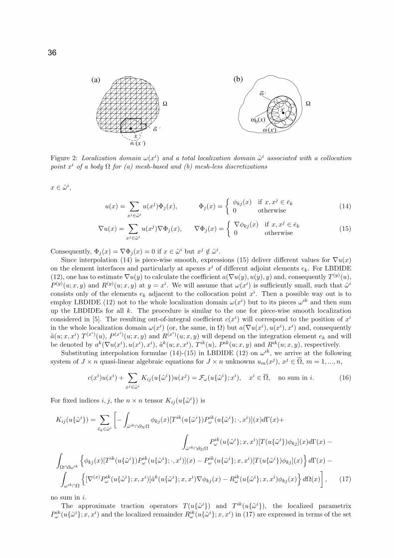
x i

(x i)

i

(a)~

(xi)

i

xi

0(x)

(b)

Figure 2: Localization domain ω(xi) and a total localization domain ωi associated with a collocationpoint xi of a body Ω for (a) mesh-based and (b) mesh-less discretizations

x ∈ ωi,

u(x) =∑

xj∈ωi

u(xj)Φj(x), Φj(x) =

φkj(x) if x, xj ∈ ek

0 otherwise(14)

∇u(x) =∑

xj∈ωi

u(xj)∇Φj(x), ∇Φj(x) = ∇φkj(x) if x, xj ∈ ek

0 otherwise(15)

Consequently, Φj(x) = ∇Φj(x) = 0 if x ∈ ωi but xj /∈ ωi.Since interpolation (14) is piece-wise smooth, expressions (15) deliver different values for ∇u(x)

on the element interfaces and particularly at apexes xi of different adjoint elements ek. For LBDIDE(12), one has to estimate ∇u(y) to calculate the coefficient a(∇u(y), u(y), y) and, consequently T (y)(u),P (y)(u;x, y) and R(y)(u;x, y) at y = xi. We will assume that ω(xi) is sufficiently small, such that ωi

consists only of the elements ek adjacent to the collocation point xi. Then a possible way out is toemploy LBDIDE (12) not to the whole localization domain ω(xi) but to its pieces ωik and then sumup the LBDIDEs for all k. The procedure is similar to the one for piece-wise smooth localizationconsidered in [5]. The resulting out-of-integral coefficient c(xi) will correspond to the position of xi

in the whole localization domain ω(xi) (or, the same, in Ω) but a(∇u(xi), u(xi), xi) and, consequentlya(u;x, xi) T (xi)(u), P (xi)(u;x, y) and R(xi)(u; x, y) will depend on the integration element ek and willbe denoted by ak(∇u(xi), u(xi), xi), ak(u;x, xi), T ik(u), P ik(u;x, y) and Rik(u;x, y), respectively.

Substituting interpolation formulae (14)-(15) in LBDIDE (12) on ωik, we arrive at the followingsystem of J × n quasi-linear algebraic equations for J × n unknowns um(xj), xj ∈ Ω, m = 1, ..., n,

c(xi)u(xi) +∑

xj∈ωi

Kij(uωi)u(xj) = Fω(uωi; xi), xi ∈ Ω, no sum in i. (16)

For fixed indices i, j, the n × n tensor Kij(uωi) is

Kij(uωi) =∑

ek∈ωi

[−

∫ωik∩∂NΩ

φkj(x)[T ik(uωi)P ikω (uωi; ·, xi)](x)dΓ(x)+

∫ωik∩∂DΩ

P ikω (uωi; x, xi)[T (uωi)φkj ](x)dΓ(x) −∫

Ω∩∂ωik

φkj(x)[T ik(uωi)P ik

ω (uωi; ·, xi)](x) − P ikω (uωi; x, xi)[T (uωi)φkj ](x)

dΓ(x) −∫

ωik∩Ω

[∇(x)P ik

ω (uωi; x, xi)]ak(uωi; x, xi)∇φkj(x) − Rikω (uωi; x, xi)φkj(x)

dΩ(x)

], (17)

no sum in i.The approximate traction operators T (uωi) and T ik(uωi), the localized parametrix

P ikω (uωi; x, xi) and the localized remainder Rik

ω (uωi; x, xi) in (17) are expressed in terms of the set

36

of unknowns uωi := u(xj), xj ∈ ωi. The expressions are obtained after substituting interpolationformulae (14), (15) for u in the coefficient a(u; ·) in the definitions for T (u), T (y)(u), P

(y)ω (u;x, y)

and R(y)ω (u;x, y). The right hand side components Fω(uωi, xi) in (16) are obtained after similar

employing interpolation formulae (14), (15) for u in (13).Note that the term with Rik

ω disappears in the last integral in the right hand side of (17) if theparametrix P ik

ω (x, xi) is given by (10). On the other hand, if the cut-off function χ(x, xi) and itsnormal derivative are equal zero at x on the boundary ∂ω(xi), then the part of the third integral alongΩ ∩ ∂ω(xi) disappears in the right hand side of (17).

Mesh–less discretization For a mesh–less discretization, one needs a method of local interpo-lation or approximation of a function along randomly distributed nodes xi. We will suppose all theapproximation nodes xi belong to Ω and will use them also as collocation points for the LBDIDEsdiscretization. Let, as before, J be the total number of nodes xj (i = 1, 2, ..., J). Let us considera mesh–less method, for example, the moving least squares (MLS) (see e.g. [14]), that leads to thefollowing approximation of a function u(x)

u(x) =∑

xj∈ω0(x)

u(xj)Φj(x), x ∈ Ω. (18)

Here Φj(x) are known smooth shape functions such that Φj(x) = 0 if xj /∈ ω0(x), ω0(x) is a localizationdomain of the approximation formula, and u(xj) are unknown values of an auxiliary function u(x) atthe nodes xj , that is, the so-called δ−property is not assumed for approximation (18).

Let ω(xi) be a localization domain around a node xi. Then for any x ∈ ω(xi), the total approxi-mation of u(x) can be written in the following local form,

u(x) =∑

xj∈ωi

u(xj)Φj(x), ∇u(x) =∑

xj∈ωi

u(xj)∇Φj(x), x ∈ ω(xi), (19)

where ωi := ∪x∈ω(xi)∩Ωω0(x) is a total localization domain, Fig. 2(b). Consequently, Φj(x) =∇Φj(x) = 0 if x ∈ ω(xi) and xj /∈ ωi. Let Jωi be the number of nodes xj ∈ ωi and uωi bethe array of the function values u(xj) at the node points xj ∈ ωi. Since our approximation (19) for uis smooth, its gradient approximation in (19) is continuous.

After substitution of approximation (19) in LBDIDE (12), we arrive at the following system ofquasi-linear system of J × n algebraic equations with respect to J × n unknowns um(xj), xj ∈ Ω,m = 1, ..., n,∑

xj∈ωi

[c(xi)Φj(xi) + Kij(uωi)

]u(xj) = Fω(uωi, xi), xi ∈ Ω, no sum in i. (20)

For any i, j, the n × n tensor Kij in (20) is

Kij(uωi) = −∫

ω(xi)∩∂NΩΦj(x)[T (xi)(uωi)P (xi)

ω (uωi; ·, xi)](x)dΓ(x)+∫ω(xi)∩∂DΩ

P (xi)ω (uωi; x, xi)[T (uωi)Φj ](x)dΓ(x) −∫

Ω∩∂ω(xi)

Φj(x)[T (xi)(uωi)P (xi)

ω (uωi; ·, xi)](x) − P (xi)ω (uωi; x, xi)[T (uωi)Φj ](x)

dΓ(x) −∫

ω(xi)∩Ω

[∇(x)P (xi)

ω (uωi; x, xi)]a(uωi; x, xi)∇Φj(x) − R(xi)ω (uωi;x, xi)Φj(x)

dΩ(x), (21)

with the shape functions Φj from (19). Expressions for T (uωi), Pω(uωi;x, xi) and Rω(uωi;x, xi)in terms of the set of unknowns uωi := u(xj), xj ∈ ωi are obtained after substituting interpolationformulae (19) for u in the coefficient a(u; ·) in the definitions for T (u), Pω(u;x, y) and Rω(u;x, y). Theright hand side components Fω(uωi, xi) are obtained after similar employing interpolation formulae(19), for u in (13).

Advances in Boundary Element Techniques V 37

Conclusion

From the definitions in both mesh based and mesh–less methods, we have φkj(x) = ∇φkj(x) =Φj(x) = ∇Φj(x) = [T (u)φkj ](x) = [T (y)(u)φkj ](x) = [T (u)Φj ](x) = [T (y)(u)Φj ](x) = 0 if x ∈ ω(xi)but xj /∈ ωi. Consequently Kij = 0 if xj /∈ ωi, and moreover, Kij depend only on uωi or uωi,respectively. Thus, each equation in (16) and (20) has not more than Jωi ×n J×n non-zero entries,i.e. the systems are sparse.

The second kind structure of the nonlinear LBDIDE and of the corresponding mesh-based discretesystem look very promising for constructing simple and fast converging iteration algorithms of itssolution without preconditioning, thus outperforming other available numerical techniques.

References

[1] C.A. Brebbia , J.C.F. Telles and L.C. Wrobel, Boundary Element Techniques, Springer (1984).

[2] P.K. Banerjee, The Boundary Element Methods in Engineering, McGraw-Hill (1994).

[3] M.H. Aliabadi, The Boundary Element Method, Vol. 2, Applications in Solids and Structures,Wiley (2002).

[4] X.-W. Gao, T.G. Davies, Boundary Element Programming in Mechanics, Cambridge Univ. Press(2002).

[5] S.E. Mikhailov, Engineering Analysis with Boundary Elements, 26, 681–690 (2002).

[6] S.E. Mikhailov and I.S. Nakhova, In: S. Amini (Ed.) Fourth UK Conference on Boundary IntegralMethods, Salford University, 175-184 (2003).

[7] S.E. Mikhailov, In: C.Constanda, M.Ahues & A.Largillier (Eds) Integral Methods in Science andEngineering: Analytic and Numerical Techniques, Birkhauser, 139-144 (2004).

[8] S.E. Mikhailov, In: R.Gallego and M.H.Aliabadi (Eds) Advances in Boundary Element TechniquesIV. Queen Mary, Univ. of London, 289-294 (2003).

[9] J. Sladek, V. Sladek and S. N. Atluri, Computational Mechanics, 24, 456-462 (2000).

[10] J.L. Synge, Hypercircle in Mathematical Physics, Cambridge Univ. Press (1957).

[11] S.M.Vogel and F.J.Rizzo, J.Elast., 3, 203-216 (1973).

[12] R.B. Wilson and T.A.Cruse, Intern. J. Numer. Methods. Eng., 12, 1383-1397 (1978).

[13] C. Miranda, Partial Differential Equations of Elliptic Type, Springer (1970).

[14] T. Belytschko, Y. Krongauz, D. Organ, M. Flemming, and P. Krysl, Comput. Methods Appl.Mech. Engrg. 139, 4–47 (1996).

38

On the Transient Wave Propagation Phenomena at 2D Half-SpaceSurfaces and Rigid Foundations Response

Euclides Mesquita1, Luiz H. Thomazo2 and Persio L.A. Barros3

1 Dept. of Computational Mechanics, Unicamp, Brazil

email: euclides@fem.unicamp.br

2 Dept. of Computational Mechanics, Unicamp, Brazil

email: luth@fem.unicamp.br

3 Dept. of Transportation and Geotechnique, Unicamp, Brazil

Keywords: Boundary element method, transient response, two-dimensional rigid surfacefoundations, viscoelastic half-space, wave propagation

Abstract. In this article the transient response of a 2D rigid and massless foundation resting on a half-

space surface is correlated to the wave propagation phenomena occurring along the soil-foundation

interface. The rigid foundation transient response is determined using a numerically synthesized

viscoelastic auxiliary state, incorporated in an indirect version of the Boundary Element Method (IBEM).

The rigid foundation response is obtained by imposing the standard equilibrium and point-wise kinematic

compatibility condition at the soil-foundation interface. A numerical analysis of the transient wave

propagation phenomena at the half-space surface indicates that traction loads generate dilatational, shear

and Rayleigh waves at every load discontinuity. These multiple waves impinge the points, at which rigid

foundation kinematic compatibility is prescribed, leading to abrupt oscillations in the transient response.

The results obtained in the present work suggest that the short time transient response of 2D rigid

foundations is strongly influenced by the wave propagation phenomena along the soil-foundation

interface.

Introduction

In the previous years the authors of the present article have been concerned with the numerical synthesis

of stationary and transient stress boundary value problems (SBVPs) of viscoelastodynamics which can be

regarded as auxiliary states and be incorporated in the Boundary Element Method (BEM). It should be

noted that to describe the dynamic response of bounded or unbounded viscoelastic domains by integral

equations requiring only boundary discretization domain, a viscoelastic auxiliary solution is required. For

the stationary case, a viscoelastodynamic solution may be obtained from the corresponding elastodynamic

solution, by applying the elastic-viscoelastic correspondence principle [1]. On the other hand, a general

transient viscoelastic auxiliary state does not exist. The authors of this article have numerically

synthesized stationary viscoelastic auxiliary states for 2D isotropic and anisotropic full-spaces and half-

spaces, [2]. More recently, transient auxiliary solutions for viscoelastic half-spaces have been numerically

synthesized using the Fast Fourier Transform (FFT) algorithm in conjunction with accurate strategies for

integrating stationary solutions at very high frequencies [3]. These transient solutions may be incorporated

in the BEM to analyze the dynamics of rigid surface foundations interacting with viscoelastic soils and

subjected to transient excitations.

This outlined solution methodology has been implemented and an analysis of the short time response of

rigid and massless foundations show several oscillations for which there was no apparent explanation. So

the main purpose of this article is to investigate the transient wave propagation phenomena originated by

Advances in Boundary Element Techniques V 39

the non-singular viscoelastic half-space solutions and to correlate this propagation pattern with the short

time response of the rigid foundations.

The stationary problem

Formulation. The stationary SBPV being addressed is governed by the Navier operator:

* * * 2

, ,i jj j ji iu u u (1)

In equation (1) is the circular frequency, is the continuum density, *, * are complex Lame´s

constants, incorporating the viscoelastic effects and defined by * 1 i ( ) and * 1 i ( ) , with

being the damping factor. The boundary conditions, determining the half-space auxiliary state, consists of

a vertical constant traction distribution applied at the half-space surface S, shown in figure 1, and

described by:

when, 0

0 when

z

z

t x at x z

x a(2)

0 25 50 75 100 125 150-8

-6

-4

-2

0

2

Ao

Log[uzz(Ao)]

REALIMAG

Figure 1: Auxiliary state - definitions Figure 2: Stationary solution uzz

Solution. The stationary problem is solved with the aid of the Fourier Integral Transform. The inverse

transform is computed numerically. The complete expressions for the half-space displacement and

tractions may be found in [2]. The typical expression rendering the displacements uij at a point xi

displacements at the half-space, due to loaded area with center at xj (see fig.1) is an improper integral with

the following structure:

iju , , , , , , , , , , , , expi j ij i j jx x z H x x z k t x k ixk dk (3)

In equation (3) Hij(xi, xj, z, , k, , , , ) is the kernel of the stationary viscoelastic solution to be found

in [2], tj ( , x, k) are the surface tractions written in the wave number domain k. An integration strategy,

based on the Longman algorithm [4] for improper integration, combined with an adaptive quadrature

scheme [5] was developed to perform the integrations shown in equation (3).

Figure 2 shows a typical displacement solution for the stationary case, given as a function of the

dimensionless frequency parameter is A0= a/cS, in which a is the load half-width and cS=( / )1/2 is the

shear wave velocity of the elastic continuum. An analysis of figure 2 shows that the implemented

40

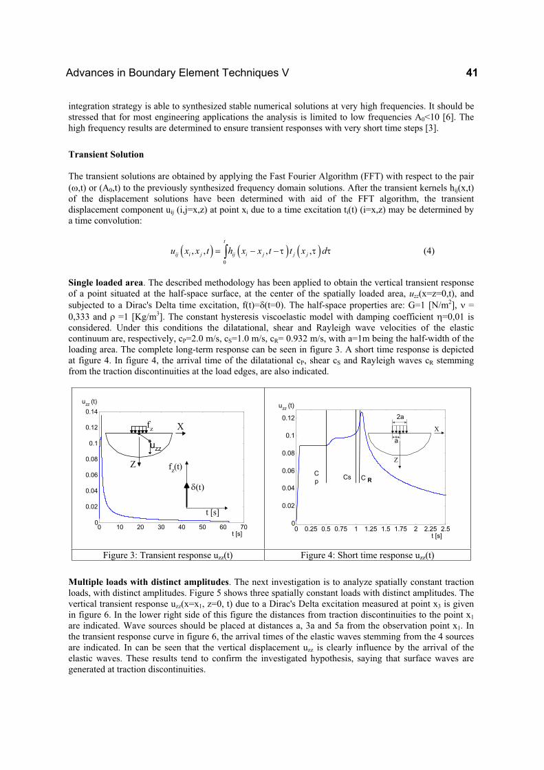
integration strategy is able to synthesized stable numerical solutions at very high frequencies. It should be

stressed that for most engineering applications the analysis is limited to low frequencies A0<10 [6]. The

high frequency results are determined to ensure transient responses with very short time steps [3].

Transient Solution

The transient solutions are obtained by applying the Fast Fourier Algorithm (FFT) with respect to the pair

( ,t) or (A0,t) to the previously synthesized frequency domain solutions. After the transient kernels hij(x,t)

of the displacement solutions have been determined with aid of the FFT algorithm, the transient

displacement component uij (i,j=x,z) at point xi due to a time excitation ti(t) (i=x,z) may be determined by

a time convolution:

0

, , , ,

t

ij i j ij i j j ju x x t h x x t t x d (4)

Single loaded area. The described methodology has been applied to obtain the vertical transient response

of a point situated at the half-space surface, at the center of the spatially loaded area, uzz(x=z=0,t), and

subjected to a Dirac's Delta time excitation, f(t)= (t=0). The half-space properties are: G=1 [N/m2], =

0,333 and =1 [Kg/m3]. The constant hysteresis viscoelastic model with damping coefficient =0,01 is

considered. Under this conditions the dilatational, shear and Rayleigh wave velocities of the elastic

continuum are, respectively, cP=2.0 m/s, cS=1.0 m/s, cR= 0.932 m/s, with a=1m being the half-width of the

loading area. The complete long-term response can be seen in figure 3. A short time response is depicted

at figure 4. In figure 4, the arrival time of the dilatational cP, shear cS and Rayleigh waves cR stemming

from the traction discontinuities at the load edges, are also indicated.

0 10 20 30 40 50 60 700

0.02

0.04

0.06

0.08

0.1

0.12

0.14

t [s]

uzz

(t)

fz

uzz

Z

X

fz(t)

t [s]

t

0 0.25 0.5 0.75 1 1.25 1.5 1.75 2 2.25 2.50

0.02

0.04

0.06

0.08

0.1

0.12

t [s]

uzz

(t)

C

pCs C R

a

2a

Z

Xtt

Figure 3: Transient response uzz(t) Figure 4: Short time response uzz(t)

Multiple loads with distinct amplitudes. The next investigation is to analyze spatially constant traction

loads, with distinct amplitudes. Figure 5 shows three spatially constant loads with distinct amplitudes. The

vertical transient response uzz(x=x1, z=0, t) due to a Dirac's Delta excitation measured at point x3 is given

in figure 6. In the lower right side of this figure the distances from traction discontinuities to the point x1

are indicated. Wave sources should be placed at distances a, 3a and 5a from the observation point x1. In

the transient response curve in figure 6, the arrival times of the elastic waves stemming from the 4 sources

are indicated. In can be seen that the vertical displacement uzz is clearly influence by the arrival of the

elastic waves. These results tend to confirm the investigated hypothesis, saying that surface waves are

generated at traction discontinuities.

Advances in Boundary Element Techniques V 41

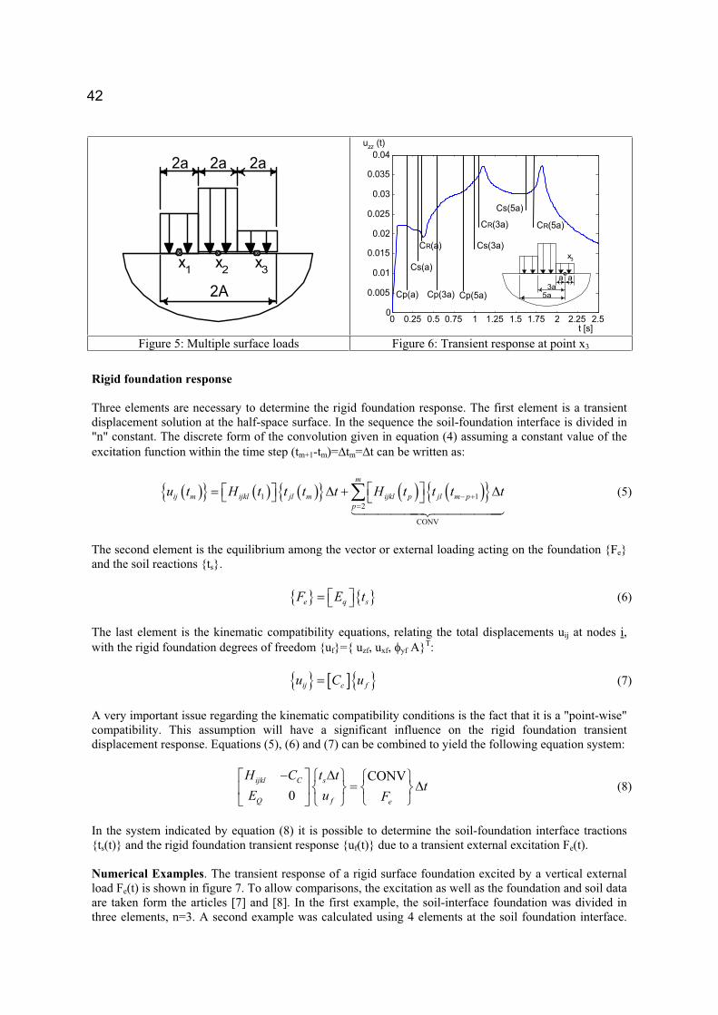
2A

2a

x

1x

2x3

2a2a

0 0.25 0.5 0.75 1 1.25 1.5 1.75 2 2.25 2.50

0.005

0.01

0.015

0.02

0.025

0.03

0.035

0.04

t [s]

uzz

(t)

Cp(a) Cp(3a) Cp(5a)

Cs(a)

Cs(3a)

Cs(5a)

CR(a)

CR(3a) CR(5a)

3a

a

5a

a

x3

Figure 5: Multiple surface loads Figure 6: Transient response at point x3

Rigid foundation response

Three elements are necessary to determine the rigid foundation response. The first element is a transient

displacement solution at the half-space surface. In the sequence the soil-foundation interface is divided in

"n" constant. The discrete form of the convolution given in equation (4) assuming a constant value of the

excitation function within the time step (tm+1-tm)= tm= t can be written as:

1 1

2

CONV

m

ij m ijkl jl m ijkl p jl m p

p

u t H t t t t H t t t t (5)

The second element is the equilibrium among the vector or external loading acting on the foundation Fe

and the soil reactions ts.

e q sF E t (6)

The last element is the kinematic compatibility equations, relating the total displacements uij at nodes i,

with the rigid foundation degrees of freedom uf= uzf, uxf, yf AT:

ij c fu C u (7)

A very important issue regarding the kinematic compatibility conditions is the fact that it is a "point-wise"

compatibility. This assumption will have a significant influence on the rigid foundation transient

displacement response. Equations (5), (6) and (7) can be combined to yield the following equation system:

CONV

0

ijkl C s

Q f e

H C t tt

E u F(8)

In the system indicated by equation (8) it is possible to determine the soil-foundation interface tractions

ts(t) and the rigid foundation transient response uf(t) due to a transient external excitation Fe(t).

Numerical Examples. The transient response of a rigid surface foundation excited by a vertical external

load Fe(t) is shown in figure 7. To allow comparisons, the excitation as well as the foundation and soil data

are taken form the articles [7] and [8]. In the first example, the soil-interface foundation was divided in

three elements, n=3. A second example was calculated using 4 elements at the soil foundation interface.

42

The transient responses of the rigid foundations considering 3 and 4 elements, are given in figures 7 and 8,

respectively. It can be seen that the foundation peaks are related to the arrival of the Rayleigh surface

waves at the points used to establish rigid body kinematic compatibility.

0 0.2 0.4 0.6 0.8 10

0.2

0.4

0.6

0.8

1

t [s x10-3]

uzz

(t) [m x10-6]

0 0.2 0.4 0.6 0.8 10

0.2

0.4

0.6

0.8

1

Cp(a)

Cp(3a)

Cp(5a)

Cs(a)

Cs(3a)

Cs(5a)

CR(5a)

Cr(3a)

CR(a)

X

Z

Fextz

3a5a

a

0 0.2 0.4 0.6 0.8 10

0.2

0.4

0.6

0.8

1

t [s x10-3]

uzz

(t) [m x10-6]

a

3a

5a

7a

a3a 5a X

Z

Fextz

7a

Figure 8: Transient response with 3 elements Figure 9: Transient response with 4 elements

Comparisons with other authors. The pioneering works on the transient solution of 2D rigid foundations

interacting with unbounded half-spaces using the BEM were performed by Spyrakos and Antes [7] and by

Spyrakos and Beskos [8]. Figure 10 shows the transient responses obtained by [7] and [8]. The results

determined by the present authors, using 3 and 4 elements are also given in the figure.

0 0.2 0.4 0.6 0.8 10

0.2

0.4

0.6

0.8

1

t [s x10-3]

uzz

(t) [m x10-6]

IBEM - 3IBEM - 4Spyrakos e Antes

Spyrakos e Beskos

Figure 10: Transient response of rigid foundation - comparisons with other authors

The results of Spyrakos and Antes [7] only present oscillations at the very initial time instants. The

response peak does not occur at the initial time step, but rather at the time when the dilatational wave

arrives at the first node used in the compatibility equation. After this instant, the solution decays

monotonically. The maximum determined response period was Tmax=0.6x10-6s. On the other hand the

results from Spyrakos and Beskos [8], do present oscillations that may well be due to the passage of waves

at the nodes considered for kinematic compatibility.

It is not possible to assert that the oscillations present at the results reported by [7] and [8] are due to the

relation between wave propagation at the soil-foundation interface and the displacement induced at the

nodes used to establish the rigid body kinematic compatibility. What can be said is that, in the results

Advances in Boundary Element Techniques V 43

obtained by the methodology described in this article, which allows much finer or smaller time steps, the

wave propagation at the soil-foundation interface creates oscillations and peaks. Increasing the number of

elements under the foundation may diminish the effect of this phenomenon. Another possibility is to

establish kinematic compatibility not in an instantly and point-wise manner. The displacement used in the

compatibility relation could be an average of the displacement under the element. This would reduce the

influence of the displacement peaks related to the impinging of the Rayleigh waves.

Concluding remarks

In this article a transient stress boundary value problem of viscoelastodynamics is numerically solved. The

transient displacements caused by distributed loads applied at the half-space surface submitted to a Dirac's

Delta excitation is determined with good accuracy and for very small time steps. A numerical

investigation is carried out to confirm the hypothesis, which suggested that elastic waves are generated at

surface load discontinuities. The suggested hypothesis was confirmed in numerical results.

Furthermore, the transient displacement solution was used, in conjunction with equilibrium equations and

kinematic compatibility restrictions to yield the transient response of rigid and massless 2D foundations.

The rigid foundation transient displacement response presented a series of peaks and oscillations. Through

a numerical investigation it was possible to establish that these oscillations were intimately related to the

arrival of the elastic waves propagating along the soil-foundation interface at the nodes used to determine

the rigid body kinematic compatibility. The reasons for the displacement peaks and oscillations were

clarified. The synthesized transient results were compared to those obtained by the pioneering transient

analysis using the BEM [7,8]. Comparisons could furnish a basis that would explain some of the

oscillations present in the mentioned pioneering works.

Acknowledgements

This research has been supported, throughout the years, by the following funding agencies: Fapesp, CNPq,

Capes and FAEP/UNICAMP. This is greatfully acknowledged.

References

[1] Christensen, R. M., 1982, Theory of Viscoelasticity, Academic Press, NY

[2] Almeida Barros, P. L., Mesquita, E., 1999, Elastodynamic Green’s Functions for Orthotropic Plane

Strain Continua with inclined Axis of Symmetry, International Journal for Solids and Structures, vol.

36, pp. 4767-4788.

[3] Mesquita, E, Adolph, M; Almeida Barros, PL; Romanini, E, (2002a): Transient Green and Influence

Functions for Plane Strain Visco-Elastic Half-Spaces. Proceedings of the IABEM SYMPOSIUM

2002, The University of Texas at Austin, Texas, May 28-31, 2002, pp.1-12.

[4] Longman, I. M. (1956) Note on method for computing infinite integrals of oscillatory functions.

Cambridge Philosophical Society, Vol. 52, pp. 764-768.

[5] Forsythe, G.E. (1977), Computer Methods for Mathematical Computations, Prentice Hall.

[6] Gazetas, G, (1983), Analysis of Machine Foundation Vibrations: State of the Art. Soil Dynamics and

Earthquake Engineering, vol. 2, pp. 2-42.

[7] Spyrakos, C. C, Antes, H., 1986, Time Domain Boundary Element Method Approaches in

Elastodynamics: A Comparative Study, Computers & Structures, vol. 24, n. 4, pp. 529-535.

[8] Spyrakos, C. C., Beskos, D. E., 1986, Dynamic Response of Rigid Strip-Foundations by a Time-

Domain Boundary Element Method, International Journal for Numerical Methods in Engineering,

vol. 23, pp. 1547-1564.

44

Advances in Boundary Element Techniques V 45

46

Advances in Boundary Element Techniques V 47

48

3D Quadrilatera l linear elem ents

0

50

100

150

200

250

300

0 10000 20000 30000 40000 50000 60000 70000

NDOFT2 / NDOFC

Co

nd

en

se

d / N

on

-co

nd

en

se

d C

PU

Tim

e

Advances in Boundary Element Techniques V 49

3 D L in e a r o r q ua d ra tic e le m e n ts

0 ,0

1 ,0

2 ,0

3 ,0

4 ,0

5 ,0

0 2 0 0 4 0 0 60 0 8 00 10 0 0

N D OFC

Ga

us

sL

U /

GM

RE

S

CP

U tim

e

N u l l in i t. s o l.

P re v in it. s o l.

50

!" #

$ %

% & ' (% $ ) * $ ! + , - % % .&/%

* 0 $ &

% 1 * 2 ' % * ' 2 & 2 Æ% % 3 Æ 4 1 ! ) * )

- % 1 % 5 ) 6 %7% 8 $ 9 1 % : &

) )

) * ) )

* * ) '

- & ' ; 8% * 2%

*

* ' (& ' - % 1 <

; .'/% ) $ ) % * & % *

*

% * & % ; % ) )

% %

Advances in Boundary Element Techniques V 51

!

"

# $ # % # &

# Æ # Æ% ! ' #

#

' ' ' # ! (

# % #

! ' )&* & # ' +

# $ # % # ,

# % # '

#

#

-

. ' ! !

# % # + , % + ,"%

# % #"

/ + , # % # / ' ! # ! ! # % # " ' % +

#

0

# % # " 1

$ % $ 2

3 + 0 345 $,678 + 1 ( ' ( + + .97 + )-* / 2 . : ' ' ; '

8 ' ' ),* )&* <. = . # $ ' ! 7 ' > !

! ' ; '

# $ ?

52

!

" #

$

%

&

' ( ! ! # $ !) !! ) *

+ ! ) ) !! # ! # , "

(

) )

- " ) . ! $# $# # !) ) ) ) ) $% $$% /0 ) )! )!!

- ) )

)

1

)

1 #

& /0 ! 2 )! ) !

! )

) ) !

" 3

! ) ) ! # )

/ ! 3 2 ) , % !)* !)* ) $% % !) 2 4 ) 5) ) ) ) 16 136 7 !)* , ) '! ) ! ) ) ! #&

Advances in Boundary Element Techniques V 53

!

"#

! $ % ! ! ! ! $ & ! !$ '

"# "# ! (

) * ( ( $ ' + ! !

"(# "(#

"(# "(#

",#

! (

! "#$% ! - ",# .

$ ' ! ! ( + $ ' ! . + ! /01$ 2 ! "# . ! $ &

&! ! + ! $ ' $$ ! ! ( + $

& - ! !

' "# 3 "4# 3 "4#

0 5 5

0005 55 0 ,

5 000 05 5

0005 550 005 5

5 000 05, 0, 5

5 000, 5 0 ,0

000, 0 ,

000,, 0

0 00 0 5

00 , 00,, 05

5 00 00,, 5

00 55 00,, 5

&! 6 & !7 + ! $

! 8 $ & ! 9 ! :;

54

Æ !" #

$ % &

#

'())*

+ ( , ! #

- . '/* '()* '(0* '(1* '2*

& ' * '0)*

'2* % ! '0)* Æ

. 3 . 4 % /

) 5 & ' * & ' * ' * '0(*

# ' * 674 ' * ' * ' * 674 '* ' * # '0(* ' * # 8 () # # '0(* #

# . #

Advances in Boundary Element Techniques V 55

! " ! "

#" $$%##& # ###%' #$$((' ##%')

" $$$&(# # ##$(# #$%& #'$'#

" $$$''& # #$' #$%$$ #())#

$" $$$)) # #%*$% #$%* &#*%

%" $$)*' # #$*(*% #$%(#( *)*)

'" $$(& # #'#(%( #$'&' $)&#&&

+ , -

. , / , 0!1 23 4 , 5 4 . 67 17 /

/ / . 89 : 3 !3:5

;< 2= 2 !1 2 (&*;< 56 0 >?5 25 3,@ (&%;$< 2 1 2 ! =0 = 2 )&$ )($##;%< @6 97 @A 17B 6? ? %' ' ((;'< ! A 1 1C 6 (&;*< 6 6 > 0 1 A/ @ C D @ '( ') ((';)< 2 1 = 2 &) &' ##;&< @6 17 ! " / (&*;(< 5 C ! # %&) '#$ (($;#< > ! !$ " ( %##

56

Advanced Formulation of the BIEs

for Elastic Anisotropic Materials in 2D

Vladislav Manti and Federico París

Group of Elasticity and Strength of Materials, School of Engineering University of Seville, Camino de los Descubrimientos s/n, Seville 41092 Spain

mantic@esi.us.es, paris@esi.us.es

Keywords: anisotropic elasticity, Somigliana displacement identity, Somigliana stress identity, integral kernels, free terms, strongly singular BIE, hypersingular BIE.

Abstract. Somigliana displacement and stress identities are presented in a unified way for all

linear elastic material subjected to plane strain or plane stress states. Explicit expressions of

the integral kernels and of the coefficients of the free terms are introduced in a simple novel

form which makes easy an implementation of these identities in a BEM code. The

formulation of plane anisotropic elasticity developed covers all elastic materials in plane

elastic states. In particular, both classes of mathematically non-degenerated and degenerated

materials respectively with distinct and repeated roots of the Lekhnitskii characteristic

equation are covered. The simple and explicit forms of the Lekhnitskii-Stroh matrices for

both material classes together with a novel symmetric representation of stresses introduced

provide theoretical bases for an easy deduction of expressions of the integral kernels and

coefficient tensors of the free terms in the Somigliana identities.

Introduction

The application of the Boundary Element Method (BEM) to the numerical analysis of

anisotropic elastic solids in plane elastic states started with pioneering works [1,2]. Although

since then many other advanced applications of BEM to plane elastic anisotropic problems

have been presented, still the theoretical formulation of the Boundary Integral Equations

(BIE) to be implemented in BEM codes has not been completely developed, particularly if all

linear elastic materials are considered.

The objective of the present work is to fill-in some gaps in the formulation of the two basic

BIEs, the Somigliana displacement and stress identities considered at boundary points, for

plane strain and plane stress states. Explicit expressions of the integral kernels and coefficient

tensors of the free terms in these identities with a simple and transparent structure would be in

particular very useful for advanced implementations of BEM codes.

The present work is developed in the framework of a suitable complex variable formalism

of plane anisotropic elasticity.

Lekhnitskii-Stroh Formulation of Plane Anisotropic Elasticity

Consider a fixed co-ordinate system (x1,x2,x3). Let the 3D strain-stress law of an elastic

material takes the following form in the contracted Voigt notation: eI=sIJ J (I,J=1,...,6), sIJ

defining the elastic compliances of the material. The present work is limited to materials with

a plane of elastic symmetry coincident with the coordinate plane x3=0, in-plane and out-of

plane elastic solutions being therefore uncoupled. Only in-plane solutions corresponding to

plane strain or plane stress states are analysed here. Then, the relation between in-plane

components of strains eij and stresses ij (i,j=1,2), expressed using reduced elastic

compliances, writes as:

Advances in Boundary Element Techniques V 57

stress.plane,

strain,plane,,.

233

33

12

22

11

662616

262212

161211

12

22

11

IJ

JIIJ

IJ

s

s

sss

s

sss

sss

sss

e

e

e

(1)

In the Lekhnitskii-Stroh representation of an elastic solution (see [3,4] for original works

and [5] for a modern comprehensive survey):

,)(Re2)(,)(Re2)( xBFxxAFxu (2)

displacement u and stress function vectors at a point x=(x1,x2) are given in terms of analytic

functions which define vector F(x) in the way specified later on. Stress tensor is evaluated by:

.0,1where,)(

)( 22112112a

ijaij

x

xx (3)

Complex matrices A and B verify the following Stroh orthogonality and closure relations:

,, 0ABBAKABBATTTT (4)

.Re,Re,Re2 111 0BBK0AAKIBAK TTT (5)

According to the character of complex roots (p1, p2, p3, p4) of the Lekhnitskii characteristic

polynomial

,2)2(2)( 22262

66123

164

114 spspsspspspl (6)

anisotropic materiales in plane elastic states can be classified into two groups as follows:

- the group of mathematically non-degenerate materials (ND group) when roots of l4(p)

are distinct, ,,, 241321 pppppp

- the group of mathematically degenerate materials (D group) when roots of l4(p) are

repeated, ., 4321 pppppp For isotropic and transversely isotropic materials

(x3-axis being the axis of symmetry) p1=p2=i.

As will be seen later in this section matrix B can be expressed in terms of roots of l4(p) and

matrix A in terms of the following polynomials:

.),()(,)(5.0),( 2612

261 aaaaaaaaa sspsppppssqpspqqp (7)

Multiplying eq. (2)1 by BT and eq. (2)2 by AT, an inverse relation to the representations of

eq. (2) is obtained using eq. (4):

).()()( xuBxAxKFTT (8)

In what follows particular expressions for both material groups are presented, some new

results being introduced.

ND group. Airy stress function can be expressed as x Re (z1)+ (z2) where are

analytic functions and z = z x x1+p x2. Let Imp >0 ( =1,2). Then:

,,)(

)(

22

11

dz

df

zf

zfF (9)

,11

,)()(

)()( 21

221

2121

1

2111 pp

pppp

ppBA (10)

and the corresponding normalization matrix K is expressed a:

,0)()(2)(2,,diag 21

14

2

1

222

21 ppppplBA

k

kkK (11)

where differentiation of l4(p) with respect to p has been denoted by a prime. The following

symmetric representation of the stress tensor was introduced in [6,7]:

.,)(Re2)(2

1 dz

dffzfBB jiij x (12)

58

Using the decomposition of displacements gradient into the strain tensor and the

infinitesimal rotation, ),(5.0, 1,22,1, uueu ijijji it is obtained that:

,,2lkklklkl VVVf (no summation in ) (13)

.2

22

1,

2,

2

66121611

212

2622

122

161111

ssspspV

sspV

sspV (14)

D group. Airy stress function can be expressed as x Re )()( 21 zzz where are

analytic functions and z=z x x1+px2 ( z = z x x1+ p x2), p being the root of l4 with Imp>0).

Then the following relations can be deduced:

,,)(

)()(

2

21

dz

df

zf

zfzzfF (15)

,11

,))(),(2()(

)(),(2)(

111

111 pp

pppppp

ppppBA (16)

.0)()()(,0

0 311421

2

121

22

2

ppsplppABBA kkk

kkK (17)

A symmetric representation of stress tensor, analogous to eq. (12), takes the new form:

,),(Re2)(2

1,

zzBB jiij Fx (18)

.0)(

)()()(,,)

2

2212,1,

zf

zfzfzzf

zd

d

dz

dz(z,

FFFFF (19)

Notice that F =F , is a symmetric matrix. Finally, expressions analogous to those in eqs.

(13-14) are introduced:

,0,

,,,)(

12221111

21212

1122

klkllkkl

klklklklklkl

VVVV

VfzfVfVFK (20)

).)((),)()2)(((,)(

,2

22

1,

2,

2

1611122116112

2221111121

66121611

21211

2622

12211

16111111

sspppVsppspppppVsppV

ssspspV

sspV

sspV

(21)

Integral Kernels

The following formulae of four basic Green’s (influence) functions, giving displacement and

stress function vector at x due to a point force f and a dislocation with Burgers vector b, both

applied at the origin of co-ordinates, can be deduced using eq. (5) (for the ND group this

formulation can be found in [4,5,7,8], whereas it is new for the D group):

,.)()(

)()(.

)()(

)()(Re

)(

)(

b

f

xx

xUxU

b

f

BxBGAxBG

BxAGAxAG

x

xu

u

u

TT

TT

(22)

,)(log1

),(log1

diag)( 222

121

xxxG zi

zi

for the ND group, (23)

,0)(log

)(log)()(1)(

1

2 x

xxxxG

z

zzz

i for the D group. (24)

A superscript in a Green’s function specifies the source of singularity by means of the

work-conjugated quantity. As an example,

Advances in Boundary Element Techniques V 59

2

1,

2

1,

)(Re)(and)(Re)( xxxx GABGAAU kiuikki

uik (25)

represent respectively the displacement and stress function in the i-direction, the superscript u

is indicating that these fields are caused by the work-conjugated unit force in k-direction. For

further details and physical explanations of the notation used for Green’s functions as well as

for a discussion of their symmetry properties see [7].

Due to the particularly simple expression of G in eq. (23) the so-called fundamental

solution of equations of equilibrium in displacements Uu takes the following form for the ND

group:

,)(log1

Re)(2

12

xyxy zAAi

U kiuik (26)

The other Green’s functions appearing in the Somigliana displacement and stress identities

can be derived from the above Green’s functions by differentiation [7]:

),()(),( xyyxyuijkj

uik nT where ,

)()(

a

uik

jauijk

y

xyxy (27)

,)(

)(b

iklbikl

x

UU

xyxy (28)

),()(),( xyyxy ijkljikl nT where .)(

)(ba

iklbjaijkl xy

xyxy (29)

The following simple and explicit expressions of these Green’s functions can be obtained

using the symmetric representations of stresses in eq. (12) and (18), instead of applying the

above differentiation procedure traditionally used. For the ND group:

,)(1

Re)(

,)(1

Re)(

,)(1

Re)(

2

1

22

2

1

12

2

1

12

xyxy

xyxy

xyxy

zBBBBi

zBBAi

U

zABBi

lkjiijkl

lkiikl

kjiuijk

(30)

and for the D group:

,)(Re)(

,)(Re)(

,)(Re)(

2

1,,,,

2

1,,,

2

1,,,

xyxy

xyxy

xyxy

GBBBB

GBBAU

GABB

lkjiijkl

lkiikl

kjiuijk

(31)

where derivatives of G(x)=G(z, )z are defined as follows:

,),(,),(,),( 12,2,1,zz

GzzG

z

GzzG

z

GzzG etc. (32)

yielding

,00

01),(,

0

1),(

1

22,1

12

21,

z

izz

z

zzz

izz GG (33)

60

,00

01),(,

0

21),(

2

212,2

23

211,

z

izz

z

zzz

izz GG (34)

and G ,22(z, z )=0. Notice that G , G , and G , are completely symmetric with respect to

permutation of indices , , , and .

Let a linear elastic body be defined by a domain with a finite and piecewise smooth

boundary . Let x Let r(e) and n

(e) (e=1,2) respectively be the two unit tangential and

outward normal vectors to with the origin at x (see [9,10]). Let n(y) in eqs. (27) and (29)

denote the unit outward normal vector to at y . Define B (x)=y| |y-x|< .

Coefficient Tensor of the Free Term in the Somigliana Displacement Identity

The 2nd Betti theorem of reciprocity of work, considered on the domain with an excluded

circular vanishing zone \B (x) ( 0+) for the actual elastic state and an auxiliary state

respectively defined by the following displacement and traction fields: (u, t) and (Uu, Tu),

yields the strongly singular Somigliana displacement identity for boundary points:

),(d),()()()(.v.p)()(

)(\

yxyyxyyxx

xB

uiki

uikii

uik TuUtuC (35)

where p.v. means the Cauchy principal value of the integral, the coefficient tensor of the free

term being expressed as:

,log1

Re)(2

1)2(

)1(

2 z

zAB

iC ki

uik x ),()(

)(2

)(1

)( xxeee rprz for ND group, (36)

and

,Re)(

1

2

2

1,

)(eki

uik GABC rx for D group. (37)

Formulae in eqs. (36-37) simplify to ikuikC 5.0)(x for x situated on a smooth part of .

Coefficient Tensors of the Free Terms in the Somigliana Stress Identity

Consider now the 2nd Betti theorem on \B (x) ( 0+) for the actual elastic state (u, t) and an

auxiliary state (U , T ) originated by the dislocation dipole (a kind of concentrated initial

strain) applied at x . Then using a standard asymptotic procedure [10,11] and either eqs.

(13-14) or eqs. (20-21), the following form of the hypersingular Somigliana stress identity for

boundary points can be obtained after some lengthy calculations and arrangements:

),(d),()()()(.p.f)()()()()()(

)(\

yxyyxyyxxxxxx

xB

ikliikliiuiklklijijkl TuUtuBCC (38)

where f.p. denotes the Hadamard finite part of the integral, and the coefficient tensors of the

free terms are expressed as:

,11

Re2

1)(

,log1

Re)(

,11

Relog1

Re)(

)(2

1

2

12)(2

)(

2

1)2(

)1(

2

)(2

1

2

1)(2

2

1)2(

)1(

2

ej

ee

lkjieu

ikl

lkkl

ej

eelkilkijijkl

rz

BBBBi

kB

z

zBB

iC

nz

BBAiz

zBBV

iC

x

x

x

(39)

for ND group, and

Advances in Boundary Element Techniques V 61

,Re2

1)(

,Re)(

,ReRe)(

)(2

1

2

1,,,

)(,

)(

1

2

2

1,

)(

)(2

1

2

1,,

)(,

1

2

2

1,,

)(

ej

e

elkji

euikl

elkkl

ej

e

elki

elkijijkl

rGBBBBkB

GBBC

nGBBAGBBVC

rx

rx

rrx

(40)

for D group, k(e) being the signed curvatures of at both sides of x [10]. Formulae in eqs. (39-

40) simplify to )(5.0)()( xxx klijijklC and )(0)( xx uiklkl BC for x situated on a smooth

part of .

Conclusions

Explicit expressions of the integral kernels and coefficient tensors of the free terms in the

strongly singular Somigliana displacement identity and the hypersingular Somigliana stress

identity considered at boundary points have been deduced in the framework of the complex

variable formalism of plane anisotropic elasticity. An advantage of the new expressions

presented is their relatively simple and transparent structure. These expressions can be used

for an easy development of BEM codes for plane elastic problems avoiding an

implementation of cumbersome expressions.

Acknowledgement

The authors acknowledge the financial support from the Spanish Ministry of Science and

Technology (Project MAT2003-03315).

References

[1] F.J. Rizzo and D.J. Shippy Journal of Composite Materials, 4, 36-617 (1970).

[2] T.A. Cruse and J.L. Swedlow Interactive Program for Analysis and Design Problems in

Advanced Composites Technology, Air Force Materials Laboratory, AFML-TR-71-268 (1971).

[3] S.G. Lekhnitskii Applied Mathematics and Mechanics (in Russian), 2, 345-367 (1938).

[4] A.N. Stroh Journal of Mathematical Physics, 41, 77-103 (1962).

[5] T.C.T. Ting Anisotropic Elasticity Theory and Applications, OUP (1996).

[6] V. Manti and F. París Journal of Elasticity, 47, 101-120 (1997).

[7] V. Manti and F. París Computational Mechanics, 22, 77-87 (1998).

[8] K.C. Wu, Y.T. Chiu and Z.H. Hwu Journal of Applied Mechanics, 59, 344-348 (1992).

[9] V. Manti and F. París Engnrg. Anal. Boundary Elements, 15, 283-288 (1995).

[10] V. Manti and F. París Engnrg. Anal. Boundary Elements, 16, 253-260 (1995).

[11] M. Guiggiani, G. Krishnasamy, T.J. Rudolphi and F.J. Rizzo Journal of Applied

Mechanics, 59, 604-614 (1992).

62

Mixed Shape Functions for a Poroelastic Boundary ElementFormulation

D. Pryl and M. SchanzInstitute of Applied Mechanics, Technical University Braunschweig,Spielmannstr. 11, D-38106 Braunschweig, Germany, d.pryl@tu-bs.de

Keywords: poroelasticity, mixed elements, convolution quadrature

Abstract

A Boundary Element formulation based on Biot’s theory is used to model wave prop-agation phenomena in poroelastic continua. The solid displacements ui and pore pres-sure p are chosen as a sufficient set of independent variables. The available Laplacedomain fundamental solutions can be directly employed in a Laplace domain BEMformulation. Also, these solutions are used to establish a time domain formulationbased on the Convolution Quadrature Method. Details on the latter BE formulationmay be found in [1].The spatial discretization for the solid displacements and pore pressure is performedwith the shape functions uN f

e (x) , pN fe (x) corresponding to node f of element e. The

tractions ti and flux q are handled in the same way.Up to now, in the BEM implementation identical shape functions have been applied toall quantities. In Finite Element Method, better stability of time-stepping is commonlyexperienced if the ansatz for p and q is chosen one degree lower than for ui and ti, e.g.,uN f

e (x) linear and pN fe (x) constant. Motivated by these improvements, this has been

added to the BEM implementation for both 2-d and 3-d formulations. A study aboutthe influence of the mixed shape functions on the quality of numerical results andstability of the time-stepping scheme will be presented.

Introduction

The efficiency of BEM in dealing with semi-infinite domain problems, e.g., soil-structure interaction, has long been recognized by researchers and engineers. Forsoil, a fluid saturated material, a poroelastic constitutive model should be used in con-nection with a time-dependent BE formulation to model wave propagation problemscorrectly. Dynamic poroelastic BE formulations are published in frequency domain(e.g., [2]), in Laplace domain (e.g., [3]), and in time domain [3, 4].Aiming on wave propagation problems, the time-dependent BE formulation based onthe Convolution Quadrature Method as proposed by Schanz [1] is used here.Inspired by finite elements, boundary elements employing mixed shape functionshave been implemented besides isoparametric ones. The results for isoparametric andmixed elements are compared at the example of a poroelastic column.

Advances in Boundary Element Techniques V 63

Throughout this paper, Latin indices receive the values 1,2, and 1,2,3 in two-dimensions(2-d) and three-dimensions (3-d), respectively. The Laplace transform of a function isdenoted by L f (t) = f (s).

Boundary Integral Equation

The boundary integral equation based on Biot’s theory can be written in the followingform [1] ∫ [

USi j −PS

jUF

i −PF

][tiq

]d =

∫C

[T Si j QS

j

T Fi QF

][ui

p

]d +

[ci j 00 c

][ui

p

], (1)

with solid displacements ui and pore pressure p as unknowns. Bonnet has shown thisset of unknowns is sufficient [5]. In eq (1), the total stress vector is denoted by ti andthe normal flux by q. US

i j, PSj ,U

Fi , and PF denote the Laplace domain fundamental

solutions, which can be found in [6]. Further, the domain is with boundary andseveral abbreviations T S

i j , QSj , T

Fi , and QF are introduced (for details, see [1]).

The integral free terms ci j and c in eq (1) result from the limiting behaviour of thefundamental solutions if y approaches x. A series expansion of the fundamental so-lutions with respect to r = |y− x| shows that T S

i j and QF are strongly singular andin the limit r → 0 equal to their elastostatic and acoustic counterparts, respectively.Therefore, the integral free terms ci j and c are calculated as known from elastostaticand acoustic BE formulations and the first integral on the right hand side of eq (1)has to be defined in the sense of a Cauchy Principal Value (denoted by

∫c ). The other

fundamental solutions are either regular, PSj and UF

i , or weakly singular USi j, P

F , T Fi ,

and QSj . A transformation to time domain gives, finally, the time dependent integral

equation for poroelasticity∫ [US

i j −PSj

UFi −PF

]∗[tiq

]d =

∫C

[TSi j QS

jTFi QF

]∗[ui

p

]d +

[ci j 00 c

][ui

p

](2)

with the convolution integral f ∗g =∫ t

0 f (t − )g( )d .According to the boundary element method the boundary surface is discretized byE elements e and for the state variables F polynomial shape functions N f

e (x) are de-fined. Further, the convolution integrals are approximated by the Convolution Quadra-ture Method [7]. A backward differential formula of order 2 ( denotes the quotientof its characteristic polynomials) and the parameter choice L = N and RN =

√10−10

yield the best results [8, 9]. Applying these approximations to the integral equation(2) results in the boundary element time stepping formulation for n = 0,1, . . . ,N

[ci jui (n t)c p(n t)

]=

E,F

e, f=1

n

k=0

⎡⎣ e fn−k

(US

i j,uN f

e , t)

− e fn−k

(PS

j ,pN f

e , t)

e fn−k

(UF

i ,uN fe , t

)− e f

n−k

(PF , pN f

e , t)⎤⎦[te f

i (k t)qe f (k t)

]

−⎡⎣ e f

n−k

(T Si j ,

tN fe , t

)e fn−k

(QS

j ,qN f

e , t)

e fn−k

(T Fi , tN f

e , t)

e fn−k

(QF ,qN f

e , t)⎤⎦[ue f

i (k t)pe f (k t)

].

(3)

64

The integration weights are calculated corresponding to

e fn

(US

i j, t)

=R−n

L

L−1

=0

∫US

i j

⎛⎝x,y,

(Rei 2

L

)t

⎞⎠uN fe (x)d e−in 2

L , (4)

respectively. Note, the calculation of the integration weights is only based on theLaplace transformed fundamental solutions which are available. In order to arrive ata system of algebraic equations, point collocation is used and a direct equation solveris applied.

Element Types and Ansatz Functions

During the spatial discretization, the quantities are approximated using the nodal val-ues ue f

i (t) , pe f (t) and the shape functions uN fe (x) , pN f

e (x) corresponding to the nodef of element e. For displacements ui and pore pressure p, this gives

ui (x, t) =E

e=1

F

f=1

uN fe (x)ue f

i (t) , p(x, t) =E

e=1

F

f=1

pN fe (x) pe f (t) . (5)

The tractions ti and flux q are handled in the same way. The simplest choice areisoparametric elements, i.e., taking identical ansatz functions for all quantities and thegeometry. Another option, common in finite elements for poroelasticity [10], is tochoose the ansatz for p, q one degree lower than for ui and ti, e.g., uN f

e (x), tN fe (x)

linear and pN fe (x), qN f

e (x) constant. This has been added to the BEM implementationin both 2-d and 3-d.In the numerical example, two different triangular element types are used, the linearisoparametric triangular element li-dr and the mixed triangular element lk-dr withlinear and constant ansatz functions, shown in fig. 1. Both elements have linear geom-etry and three nodes in the corners of the triangle. These are used with linear ansatz forall state variables by li-dr , but only for ui and ti by lk-dr , which has an additionalmid-element node with constant ansatz for the degrees of freedom corresponding to pand q (see tab. 1). Details may be found in [11].

Figure 1: lk-dr element

Element uN fe , tN f

epN f

e , qN fe

li-dr linear linearlk-dr linear constant

Table 1: Ansatz functions in 3-d

Advances in Boundary Element Techniques V 65

Numerical Example: 3-d Poroelastic Column

In order to investigate the differences between the two element types, a poroelasticcolumn is considered. The material data corresponding to a water saturated coarsesand (soil) can be found in Tab. 2.

K,G [ Nm2 ] Ks,Kf [ N

m2 ] , f [ kgm3 ] R [ N

m2 ] [m4

Ns ]

Soil 2.1 ·108 1.1·1010 1884 0.48 1.2 ·109 0.981 3.55·10−9

9.8 ·107 3.3·109 1000

Table 2: Material Data

21 N/m

t

t yxy

z

P

fixed end, impermeable

free end, permeable

traction free, permeable

(a) boundary conditions (b) discretization

Figure 2: Geometry, boundary conditions, and discretization of a 3-d column

The problem geometry is shown in fig. 2(a). The column of 3m (length) ×1m (height)×1m (width) is fixed and impermeable on one end, and excited by a traction jumpaccording to a unit step function ty (x, t) = 1N/m2 H (t) on the other end, which ismodelled free and permeable. The remaining surfaces are traction free and permeable(i.e., with pore pressure assumed to be zero). The geometry is discretized with 324linear triangular elements on 164 nodes, non-uniformly refined near edges and corners(see fig. 2(b)). In contrast to the isoparametric li-dr elements, where the geometry(corner) nodes are also used for all the state variables, the newly implemented mixedlk-dr elements employ them only for ui and ti and need 324 additional mid-elementnodes for p and q. Thus, there are in total 4×164 = 656 or 3×164+1×324 = 816degrees of freedom for the isoparametric or mixed elements, respectively.In Fig. 3, the displacement uy at point P at the loaded end is plotted versus time t.Fig. 4 shows the pore pressure p at point P at the supported end. Two different timestep sizes are chosen for each element type, the optimal time steps of t = 0.0005s forli-dr and t = 0.00048s for lk-dr , and additionally t = 0.001s for comparison ofboth element types with the same time step. The plots do not exhibit much differences.There seem to be no visible improvement in the displacement results, in the pressureplot a slight difference in favour of the mixed element which shows less numericaldamping can be observed. Also, the improvement in the lower stability limit t =0.0005s for li-dr and t = 0.00048s for lk-dr can not be considered substantial.At the same time, the total number of the degrees of freedom increased by a factorof about 1.2, resulting in longer computation time by a factor of 1.7, which corre-sponds to the quadratic dependence between the degrees of freedom and the numberof operations.

66

appropriate approaches to obtain a reasonable accuracy in the results for the potential in the domain, for thisnear-boundary heat transfer problem.

Acknowledgments

The first author would like to acknowledge the support received from CAPES - Coordenacao de Aperfeicoamentode Pessoal de Nivel Superior, a Brazilian Government Agency.

References

[1] M. N. Ozisik: Boundary Value Problems of Heat Conduction, Dover, 1968.

[2] C. A. Brebbia and J. Dominguez: Boundary Elements - An Introductory Course, Comp. Mech. Publ. -McGraw-Hill, Southampton, 1989.

[3] T. A. Cruse and J. D. Richardson: Self-Regularized Hypersingular BEM for Laplace’s Equation, in M.Bonnet, A. -M. Sandig and W. L. Wendland (Editors): Mathematical Aspects of Boundary ElementMethods, Chapman & Hall / CRC, Boca Raton, FL, 2000.

[4] A. B. Jorge, G. O. Ribeiro, T. A. Cruse and T. S. Fisher: Self-Regular Boundary Integral EquationFormulations for Laplace’s Equation in 2-D, Int. J. Numer. Meth. Engrg., 51 (1), pp. 1–29, 2001.

[5] T. J. Rudolphi: The use of simple solutions in the regularization of hypersingular boundary integralequations. Mathl. Comput. Modeling, 15, pp. 269–278, 1991.

[6] J. D. Richardson, T. A. Cruse, and Q. Huang: On the validity of conforming BEM algorithms for hyper-singular boundary integral equations, Int. J. Numer. Meth. Engrg., 42, pp. 213–220, 1997.

[7] V. Sladek and J. Sladek: Singular Integrals in Boundary Element Methods, Advances in Boundary Ele-ments Series, Comp. Mech. Publ. , Southampton, 1998.

[8] M. Bonnet: Boundary Integral Equation Methods for Solids and Fluids, Wiley, West Sussex, 1999.

[9] J. Dominguez, M. P. Ariza and R. Gallego: Flux and traction boundary elements without hypersingularor strongly singular integrals, Int. J. Numer. Meth. Engrg., 48, pp. 111–135, 2000.

[10] A. B. Jorge, G. O. Ribeiro and T. S. Fisher: New Approaches for Error Estimation and Adaptivity for2-D Potential Boundary Element Methods, Int. J. Numer. Meth. Engrg., 56, pp. 117-144, 2003.

[11] A. B. Jorge, T. A. Cruse, T. S. Fisher and G. O. Ribeiro: A New Variational Self-Regular Traction-BEMFormulation for Inter-Element Continuity of Displacement Derivatives, Computational Mechanics, 25, pp.466–506, 2003.

[12] J. D. Richardson and T. A. Cruse: Weakly Singular Stress-BEM for 2D Elastostatics, Int. J. Numer.Meth. Engng., 45, pp. 13–35, 1999.

Advances in Boundary Element Techniques V 67

68