SECRET SECurity of Railways against Electromagnetic … · SECurity of Railways against Electromagnetic aTtacks ... 4.3.2 Simulation results of the reference scenario 30 ... KPI Key

Deliverable D3.2 EM attack detection: parameters to control and sensors Date: 26/08/2014 Distribution: PP

Manager: IFSTTAR

SECRET

SECurity of Railways against

Electromagnetic aTtacks Grant Agreement number: 285136 Funding Scheme: Collaborative project Start date of the contract: 01/08/2012 Project website address: http://www.secret-project.eu

Deliverable D3.2 EM attack detection: parameters to control and sensors

SECRET Project Grant Agreement number: 285136

SEC-D3.2-C-08 2014-EM attack detection-IFSTTAR-final

29/08/2014 2 /44

Document details:

Title EM attack detection: parameters to control and sensors

Workpackage WP3

Date 26/08/2014

Author(s) V. Deniau, M. Aguado, C. Pinedo, M. Heddebaut

Responsible Partner IFSTTAR

Document Code SEC-D3.2-C-08 2014-EM attack detection-IFSTTAR-final

Version C

Status Final version

Dissemination level: Project co-funded by the European Commission within the Seventh Framework Programme

PU Public X

PP Restricted to other programme participants (including the Commission Services)

RE Restricted to a group specified by the consortium (including the Commission) Services)

CO Confidential, only for members of the consortium (including the Commission Services)

Document history:

Revision Date Authors Description

A1 07/07/2014 V. Deniau, C. Pinedo

First version of the report related to sub-task 3.2a and 3.2b

A2 02/08/2014 M. Aguado, C. Pinedo

Second version of chapter 4

A3 20/08/2014 V. Deniau New version of the D3.2

A4 21/08/2014 M. Heddebaut, V. Deniau

Proofreading the D3.2, update of the conclusion

A5 24/08/2014 V. Beauvois External review of A4

A6 25/08/2014 M. Heddebaut, V. Deniau

Modifications following the reviewer comments and final version



29/08/2014 3 /44

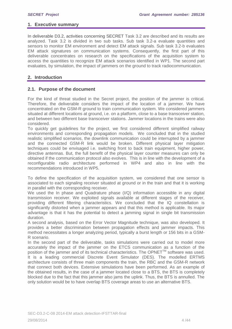
Table of content

1. Executive summary 4

2. Introduction 4

2.1. Purpose of the document 4

2.2. Definitions and acronyms 5

3. Quantities and sensors to monitor EM environment and detect EM attack signals 6

3.1. Summary of the detection methods studied in SECRET 6

3.2. EM attack detection: parameters to control 7 3.2.1 Detection by statistical spectrum analysis 7 3.2.2 Detection by quadratic analysis 9 3.2.3 Detection by time characteristics 12

3.3. EM attack detection: sensors configuration 15 3.3.1 Detection of a jamming signal on board train 15 3.3.2 Detection of a jamming signal on the track side 15 3.3.3 Jamming detection in train station 15

4. Simulation task: Analysis of the EM attack signatures on communication systems 17

4.1. Introduction 17

4.2. The simulation framework 17 4.2.1 The simulation tool: OPNET Modeler 17 4.2.2 Modelling ERTMS Architecture 19 4.2.3 Modelling attack devices 25

4.3 Reference scenario 27 4.3.1 Definition of the reference scenario 27 4.3.2 Simulation results of the reference scenario 30

4.4 Interfered scenarios 35 4.4.1 Silver Jammer 35 4.4.2 Grey Jammer 39

5. Conclusion 43

6. References 44



29/08/2014 4 /44

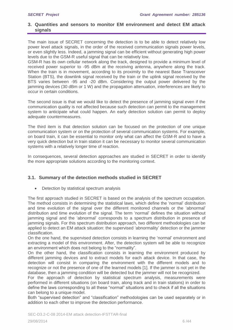
1. Executive summary

In deliverable D3.2, activities concerning SECRET Task 3.2 are described and its results are analyzed. Task 3.2 is divided in two sub tasks. Sub task 3.2-a evaluate quantities and sensors to monitor EM environment and detect EM attack signals. Sub task 3.2-b evaluates EM attack signatures on communication systems. Consequently, the first part of this deliverable concentrates on research on the specifications of the acquisition system to access the quantities to recognize EM attack scenarios identified in WP1. The second part evaluates, by simulation, the impact of jammers on the ground to track radiocommunication.

2. Introduction

2.1. Purpose of the document

For the kind of threat studied in the Secret project, the position of the jammer is critical. Therefore, the deliverable considers the impact of the location of a jammer. We have concentrated on the GSM-R ground to train communication system. We considered jammers situated at different locations at ground, i.e. on a platform, close to a base transceiver station, and between two different base transceiver stations. Jammer locations in the trains were also considered. To quickly get guidelines for the project, we first considered different simplified railway environments and corresponding propagation models. We concluded that in the studied realistic simplified scenarios, the downlink communication could be interrupted by a jammer and the connected GSM-R link would be broken. Different physical layer mitigation techniques could be envisaged i.e. switching front to back train equipment, higher power, directive antennas. But, the full benefit of the physical layer counter measures can only be obtained if the communication protocol also evolves. This is in line with the development of a reconfigurable radio architecture performed in WP4 and also in line with the recommendations introduced in WP5. To define the specification of the acquisition system, we considered that one sensor is associated to each signaling receiver situated at ground or in the train and that it is working in parallel with the corresponding receiver. We used the In phase and Quadrature phase (I/Q) information accessible in any digital transmission receiver. We exploited signals available at different stages of the receiver, providing different filtering characteristics. We concluded that the IQ constellation is significantly distorted when a jammer appears and that this method is applicable. Its major advantage is that it has the potential to detect a jamming signal in single bit transmission duration. A second analysis, based on the Error Vector Magnitude technique, was also developed. It provides a better discrimination between propagation effects and jammer impacts. This method necessitates a longer analyzing period, typically a burst length or 156 bits in a GSM-R scenario. In the second part of the deliverable, tasks simulations were carried out to model more accurately the impact of the jammer on the ETCS communication as a function of the position of the jammer and of its technical characteristics. The OPNETTM software was used. It is a leading commercial Discrete Event Simulator (DES). The modelled ERTMS architecture consists of three main components the train, the RBC and the GSM-R network that connect both devices. Extensive simulations have been performed. As an example of the obtained results, in the case of a jammer located close to a BTS, the BTS is completely blocked due to the fact that this jammer also jams the uplink. Thus, the BTS is annulled. The only solution would be to have overlap BTS coverage areas to use an alternative BTS.



29/08/2014 5 /44

2.2. Definitions and acronyms

Acronym Meaning

ATP Automatic Train Protection

BER Bit Error Rate

BSS Base Station Subsystem

BTS Base Transceiver Station

CW Continuous Wave

DES Discrete Event Simulator

ERTMS European Rail Traffic Management System

ETCS European Train Control System

EVM Error Vector Magnitude

FFT Fast Fourier Transformation

GMSK Gaussian Minimum Shift Keying

GSM-R Global System for Mobile Communications-Railway

IQ In Phase, in Quadrature of phase

ISDN Integrated Services Digital Network

KPI Key Performance Indicators

LAPB Link Access Procedure Balanced

NRZ Non-Return to Zero

NSS Network Switching Subsystem

RBC Radio Block Centre

RBW Resolution bandwidth

SNR Signal-Noise-Ratio

TDMA Time Division Multiple Access

VCO Voltage Controlled Oscillator

VTD Validated Train Data



29/08/2014 6 /44

3. Quantities and sensors to monitor EM environment and detect EM attack signals

The main issue of SECRET concerning the detection is to be able to detect relatively low power level attack signals, in the order of the received communication signals power levels, or even slightly less. Indeed, a jamming signal can be efficient without generating high power levels due to the GSM-R useful signal that can be relatively low. GSM-R has its own cellular network along the track, designed to provide a minimum level of received power superior to -95 dBm at the receiving antenna, anywhere along the track. When the train is in movement, according to its proximity to the nearest Base Transceiver Station (BTS), the downlink signal received by the train or the uplink signal received by the BTS varies between -95 and -20 dBm. Considering the output power delivered by the jamming devices (30 dBm or 1 W) and the propagation attenuation, interferences are likely to occur in certain conditions. The second issue is that we would like to detect the presence of jamming signal even if the communication quality is not affected because such detection can permit to the management system to anticipate what could happen. An early detection solution can permit to deploy adequate countermeasures. The third item is that detection solution can be focused on the protection of one unique communication system or on the protection of several communication systems. For example, on board train, it can be essential to monitor only what can affect the GSM-R and to have a very quick detection but in train station it can be necessary to monitor several communication systems with a relatively longer time of reaction. In consequences, several detection approaches are studied in SECRET in order to identify the more appropriate solutions according to the monitoring context.

3.1. Summary of the detection methods studied in SECRET

Detection by statistical spectrum analysis The first approach studied in SECRET is based on the analysis of the spectrum occupation. The method consists in determining the statistical laws, which define the ‘normal’ distribution and time evolution of the signal over the different monitored channels or the ‘abnormal’ distribution and time evolution of the signal. The term ‘normal’ defines the situation without jamming signal and the ‘abnormal’ corresponds to a spectrum distribution in presence of jamming signals. For this spectrum distribution approach, two different methodologies can be applied to detect an EM attack situation: the supervised ‘abnormality’ detection or the jammer classification. On the one hand, the supervised detection consists in learning the ‘normal’ environment and extracting a model of this environment. After, the detection system will be able to recognize an environment which does not belong to the “normality”. On the other hand, the classification consists in learning the environment produced by different jamming devices and to extract models for each attack device. In that case, the detection will consist in comparing the environment with the different models and to recognize or not the presence of one of the learned models [1]. If the jammer is not yet in the database, then a jamming condition will be detected but the jammer will not be recognized. For the approach of detection by statistical spectrum analysis, measurements were performed in different situations (on board train, along track and in train stations) in order to define the laws corresponding to all these “normal” situations and to check if all the situations can belong to a unique model. Both “supervised detection” and “classification” methodologies can be used separately or in addition to each other to improve the detection performance.



29/08/2014 7 /44

The advantage of this approach is that it can allow monitoring several communication systems in adapting the monitored frequency bands and in using adequate antennas.

Detection by quadratic analysis The second approach consists in analyzing the GMSK IQ constellation with and without jamming. This approach is based on the quadratic data received by the GSM-R terminal. Thanks to the quadratic data, we analyze the Error Vector Magnitude (EVM), which corresponds to the sum of the errors on the sample positions during one GSM-R time slot. The values reached by the EVM and the evolution of these values over the time permits to efficiently detect the presence of jamming signals. However, the method required to take into account the TDMA properties of the GSM-R in order to check if the occupied and unoccupied time slots can be used for detection. The interest of this method is that the variation of the EVM is really significant in presence of jamming signal even if the power of the jamming signal is 20 dB lower than the GSM-R signal. Then, the jamming signal could be detected even if the communication is not affected and the reaction to have could be anticipated. However, the approach has to be tested in presence of the unintentional EM noises naturally present in the railway environment. In particular, on board train the catenary-pantograph creates disturbances which can also affect the EVM but the difference with jamming signal is that the impact on the EVM is really punctual. The method has then to be tested in real railway situation to assess the risk of fault detection.

Detection by time characteristics Finally, the last method which is considered in SECRET is focused on the time characteristics of the jammers. The different jammers studied in the project work on the same principle. These devices generate ‘jamming signals’ which sweep the frequency bands dedicated to the telecommunication systems to jam. The sweeping is sufficiently quick to disturb and make impossible the establishment of the communications, in interfering with the frequency channel used by the mobile communication equipment. Measurements performed in laboratory have shown that the jamming signal is typically generated by modulating the transmitter voltage controlled oscillator (VCO) of a transmitter using a ramp signal to sweep the full targeted frequency band. Due to the VCO the jamming signal does not cover permanently all the channels but covers each frequency channel with a regular time interval. Then, the last detection principle is based on the recognition of this regular time interval.

3.2. EM attack detection: parameters to control

3.2.1 Detection by statistical spectrum analysis

The supervised detection consists in learning the ‘normal’ environment and recognizing an environment, which does not belong to the ‘normality’ and the detection by classification, which aims to recognize a jamming device, are both based on the same quantities to monitor. The basic quantity is the energy measured inside a given resolution frequency bandwidth (RBW) centered on a specific channel. However, to discriminate the presence of a jamming signal, the analysis of only one channel at a unique instant is not sufficient. So, we collect the energy over several frequency channels which define the frequency band of analysis. Moreover, several acquisitions are performed in the time to analyze the evolution of the



29/08/2014 8 /44

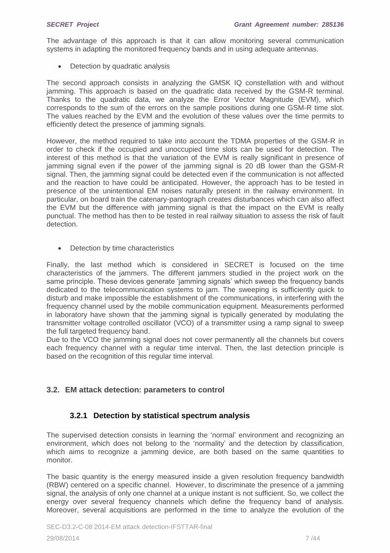
energy in time. Figure 1 Illustration of the parameters which define the acquisition dataillustrates the different parameters which define the acquisition configuration of the data to analyze.

Figure 1 Illustration of the parameters which define the acquisition data

The frequency band is defined by the first frequency (fstart), the last frequency (fstop) and the number of frequencies. However, the values of the energy obtained over each channel can be significantly depending on the resolution frequency bandwidth (RBW), notably if we are in presence of a wide band signal. The resolution frequency bandwidth corresponds to the width of the band pass around the frequencies of measurement. Knowing that the jammers produce wide frequency band interferences, this parameter has to be preliminary defined because it significantly impacts the measurement results. The RBW was fixed at 100 kHz to be similar to the band pass filter of the GSM-R terminal. Concerning the analysis of the evolution of the spectrum in time, the parameters to define are the duration of the observation and the time interval between two successive spectra. The interval between two successive collected spectra is depending of the sweep time which corresponds to the necessary time to scan the frequency band and the speed of the measurement equipment to load the data. However, the value of the sweep time is depending of the selected RBW and the number of monitored frequency channels. Moreover, the minimum sweep time can be different between different equipment. Considering the tests performed in the frame work of the SECRET project, the time to sweep the monitored frequency band was some ms for 1001 frequency steps and we collected a spectrum every 300 ms to respect the required time to load the data. Then, the data available to analyze in order to detect the presence of jamming signal can be presented as suggested in the following Figure 2.

fstart(Hz) fstop(Hz)

Resolution bandwidth (Hz)

Sweep time (s) = time to sweep the frequency band

tstart

fstart(Hz) fstop(Hz)tstart+sweep time

fstart(Hz) fstop(Hz)tstop



29/08/2014 9 /44

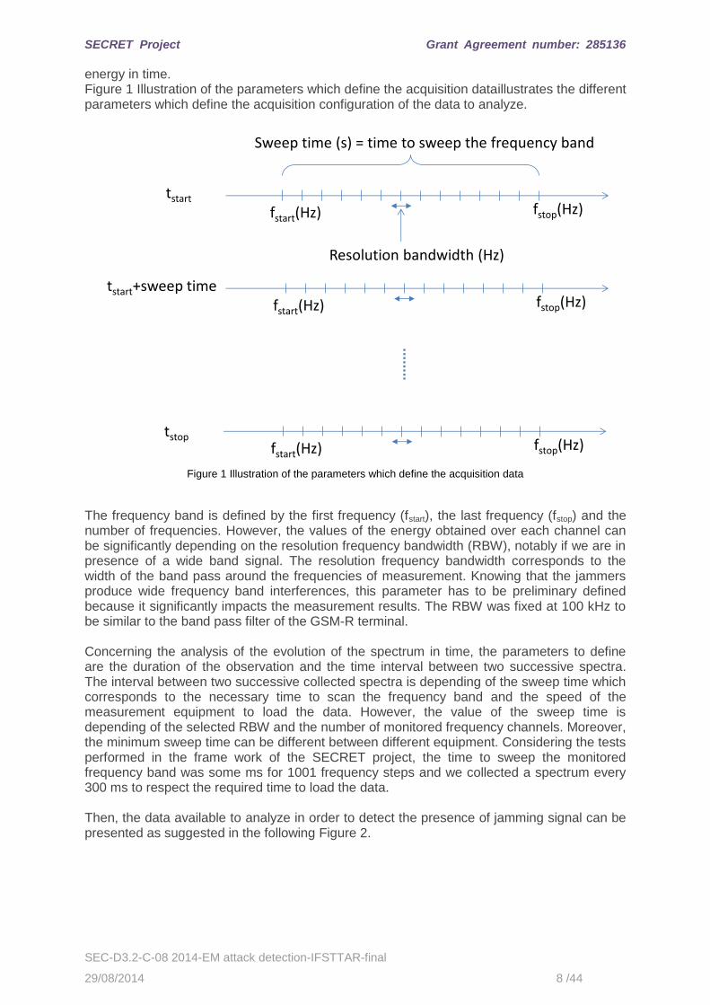
Figure 2 Illustration of the physical values on which the statistical spectrum analysis is based

Statistical laws are then expressed concerning the distribution of the energy along the time and for each frequency channel. Therefore, the supervised detection consists in comparing the law of the monitored data with the reference laws and to recognize a case which does not correspond to the reference laws. The classification method is also based on the energy on a channel inside a given resolution bandwidth. But the difference is that we collect a series of reference laws which corresponds to the distribution of the energy over the frequencies and in the time for different jammers. Then the monitored data are compared to each reference law in order to check if a jammer is recognized. In consequence, in both classification and supervised detection approaches, the quantity monitored is the energy over a frequency channel through a given bandwidth. The measurement equipment that we employed in the project is a spectrum analyser which can be configured according to the frequency band of the telecommunication system to monitor. For both methods, the learning phase to determine the reference laws were based over 900 spectra collected in varying the measurement conditions. However, the phase of detection or classification is based over only one spectrum collected every 300ms.

3.2.2 Detection by quadratic analysis

This method is focused on the detection of jamming signal able to affect the GSM-R communications. The GSM-R communication system is based on a Gaussian minimum shift keying (GMSK) modulation scheme and on a Time Division Multiple Access (TDMA). The frame data used is a NRZ (Non-Return to Zero) GSM-R burst of 156 bits transmitting during a 577 µs time slot. The GSM-R demodulation chain includes a quadratic demodulator. This detection technic is focused on the analysis of the data in the demodulation chain of the GSM-R terminal, as showed in Figure 3.

fstart=f1 f2 … … fstop

Tstart=t1 E(1,1) E(1,2) E(1,…) E(1,stop)

t2 E(2,1) E(2,2)

… E(…,1)

…

…

…

tstop E(stop,1)

RBW

ST



29/08/2014 10 /44

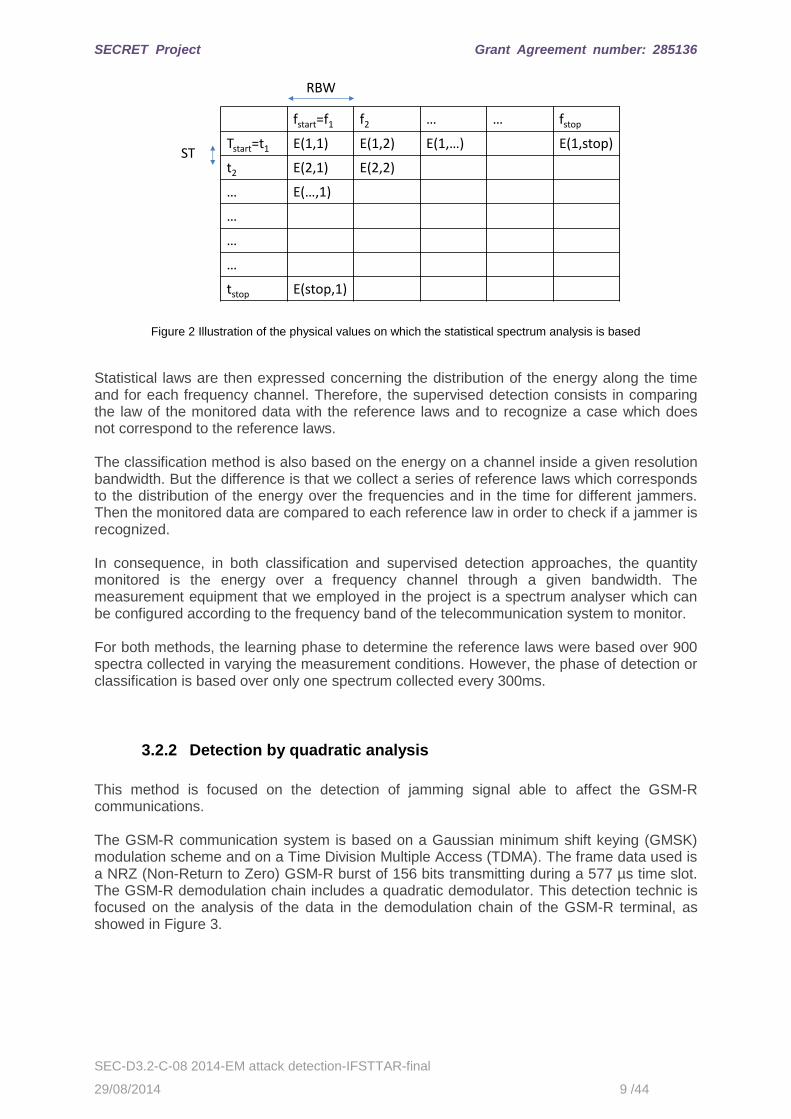
Figure 3 Illustration of the GSM-R demodulation chain

To illustrate the impact of a jamming signal on the quadratic date, the IQ constellations measured with a Rohde & Schwarz FSIQ7 Vector Signal Analyzer for a GMSK signal without jamming and with jamming are presented Figure 4.

Figure 4 “IQ” constellation of a GMSK signal (a) and of a jammed GMSK signal (b).

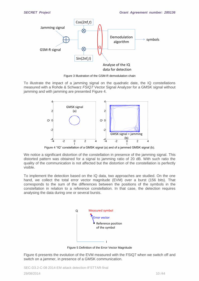
We notice a significant distortion of the constellation in presence of the jamming signal. This distorted pattern was obtained for a signal to jamming ratio of 20 dB. With such ratio the quality of the communication is not affected but the distortion of the constellation is perfectly visible. To implement the detection based on the IQ data, two approaches are studied. On the one hand, we collect the total error vector magnitude (EVM) over a burst (156 bits). That corresponds to the sum of the differences between the positions of the symbols in the constellation in relation to a reference constellation. In that case, the detection requires analysing the data during one or several bursts.

Figure 5 Definition of the Error Vector Magnitude

Figure 6 presents the evolution of the EVM measured with the FSIQ7 when we switch off and switch on a jammer, in presence of a GMSK communication.

Jamming signal

GSM-R signal

Cos(2πfct)

Sin(2πfct)

Demodulationalgorithm

symbols

Analyse of the IQ data for detection

I

Q

-4 -2 0 2 4-4

-2

0

2

4

I

Q

-4 -2 0 2 4-4

-2

0

2

4

I

Q

GMSK signal(a)

GMSK signal + jamming(b)

I

Q

Reference position of the symbol

Measured symbol

Error vector



29/08/2014 11 /44

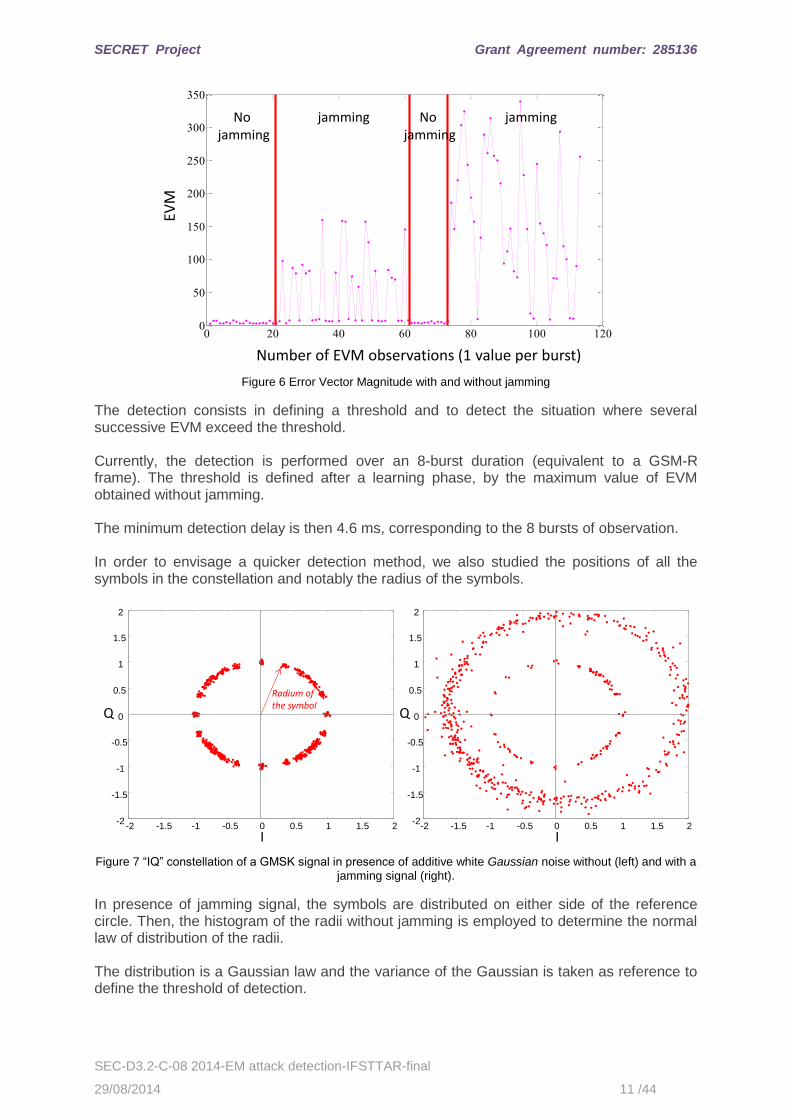
Figure 6 Error Vector Magnitude with and without jamming

The detection consists in defining a threshold and to detect the situation where several successive EVM exceed the threshold. Currently, the detection is performed over an 8-burst duration (equivalent to a GSM-R frame). The threshold is defined after a learning phase, by the maximum value of EVM obtained without jamming. The minimum detection delay is then 4.6 ms, corresponding to the 8 bursts of observation. In order to envisage a quicker detection method, we also studied the positions of all the symbols in the constellation and notably the radius of the symbols.

Figure 7 “IQ” constellation of a GMSK signal in presence of additive white Gaussian noise without (left) and with a

jamming signal (right).

In presence of jamming signal, the symbols are distributed on either side of the reference circle. Then, the histogram of the radii without jamming is employed to determine the normal law of distribution of the radii. The distribution is a Gaussian law and the variance of the Gaussian is taken as reference to define the threshold of detection.

0 20 40 60 80 100 1200

50

100

150

200

250

300

350

EVM

Number of EVM observations (1 value per burst)

No jamming

No jamming

jamming jamming

I

Q

-2 -1.5 -1 -0.5 0 0.5 1 1.5 2-2

-1.5

-1

-0.5

0

0.5

1

1.5

2

I

Q

-2 -1.5 -1 -0.5 0 0.5 1 1.5 2-2

-1.5

-1

-0.5

0

0.5

1

1.5

2

Radium of the symbol



29/08/2014 12 /44

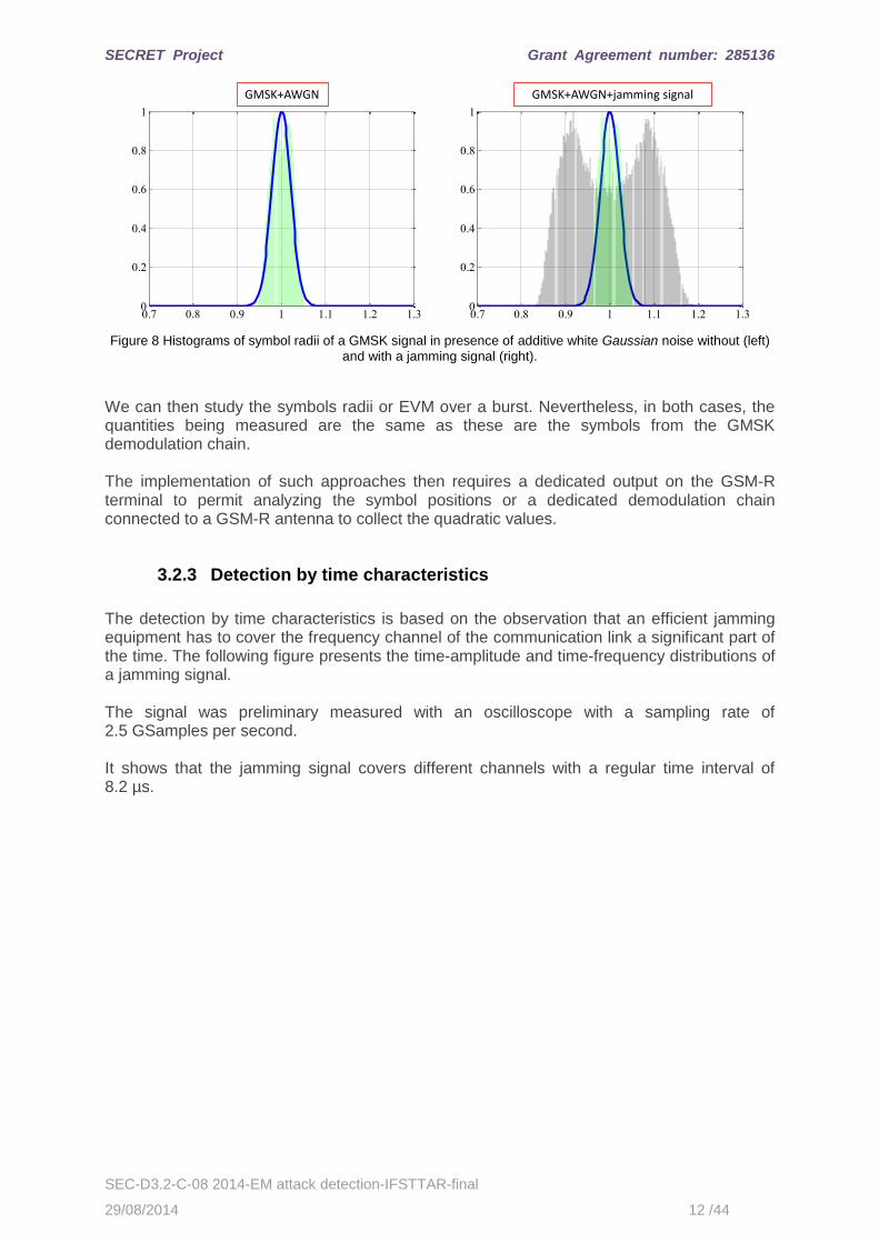
Figure 8 Histograms of symbol radii of a GMSK signal in presence of additive white Gaussian noise without (left)

and with a jamming signal (right).

We can then study the symbols radii or EVM over a burst. Nevertheless, in both cases, the quantities being measured are the same as these are the symbols from the GMSK demodulation chain. The implementation of such approaches then requires a dedicated output on the GSM-R terminal to permit analyzing the symbol positions or a dedicated demodulation chain connected to a GSM-R antenna to collect the quadratic values.

3.2.3 Detection by time characteristics

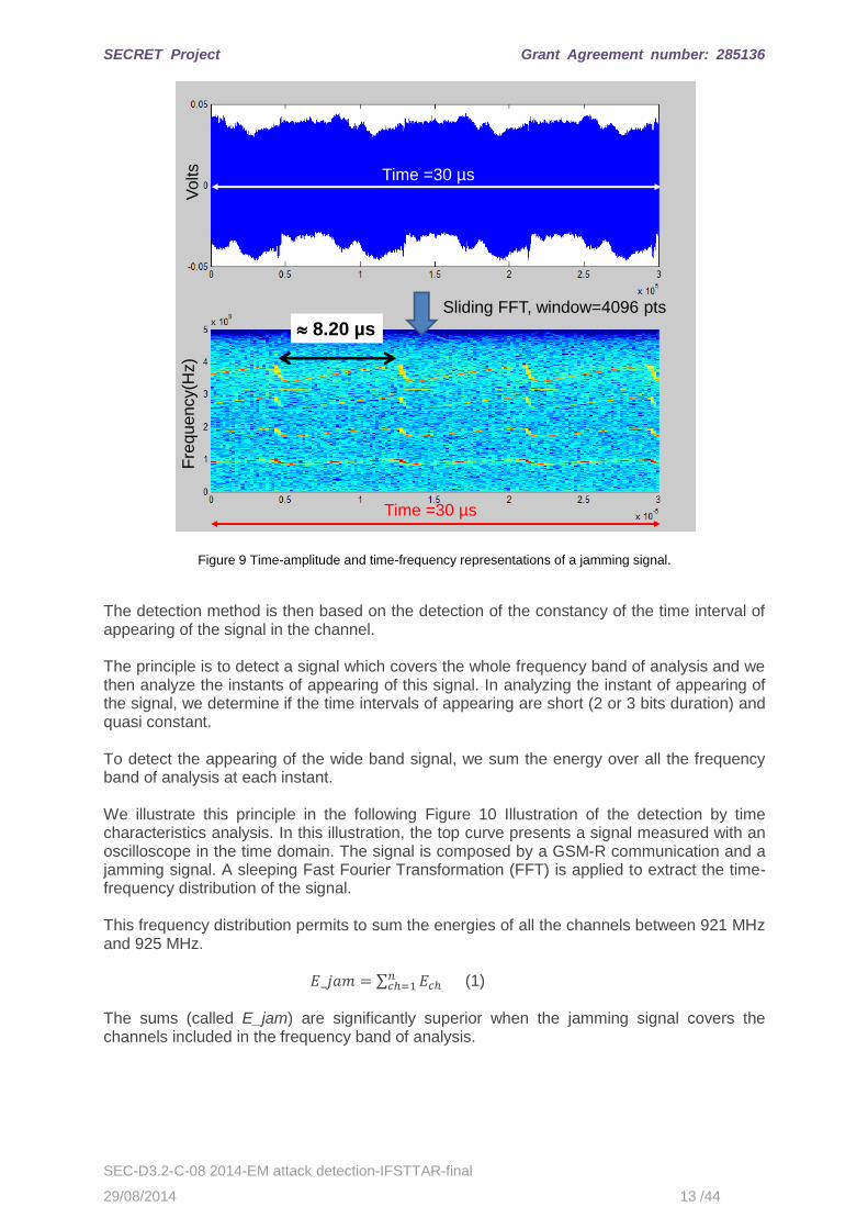
The detection by time characteristics is based on the observation that an efficient jamming equipment has to cover the frequency channel of the communication link a significant part of the time. The following figure presents the time-amplitude and time-frequency distributions of a jamming signal. The signal was preliminary measured with an oscilloscope with a sampling rate of 2.5 GSamples per second. It shows that the jamming signal covers different channels with a regular time interval of 8.2 µs.

0.7 0.8 0.9 1 1.1 1.2 1.30

0.2

0.4

0.6

0.8

1

0.7 0.8 0.9 1 1.1 1.2 1.30

0.2

0.4

0.6

0.8

1

GMSK+AWGN GMSK+AWGN+jamming signal



29/08/2014 13 /44

Figure 9 Time-amplitude and time-frequency representations of a jamming signal.

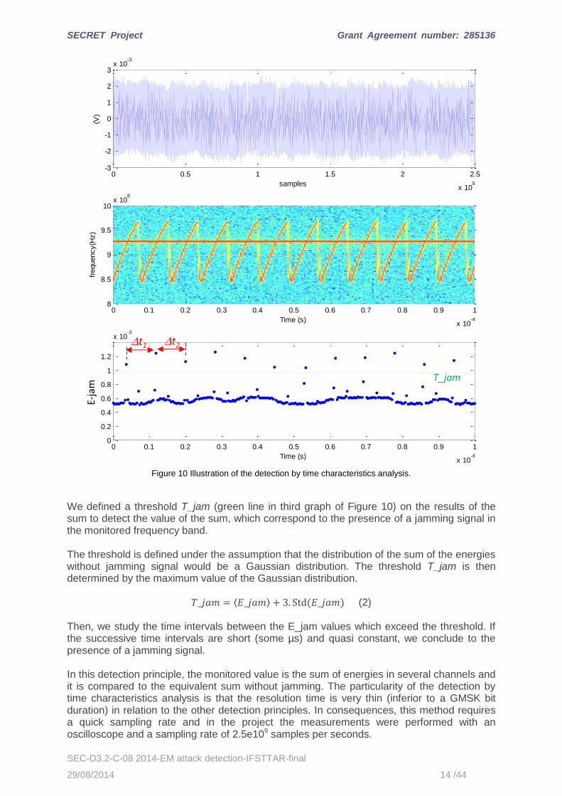
The detection method is then based on the detection of the constancy of the time interval of appearing of the signal in the channel. The principle is to detect a signal which covers the whole frequency band of analysis and we then analyze the instants of appearing of this signal. In analyzing the instant of appearing of the signal, we determine if the time intervals of appearing are short (2 or 3 bits duration) and quasi constant. To detect the appearing of the wide band signal, we sum the energy over all the frequency band of analysis at each instant. We illustrate this principle in the following Figure 10 Illustration of the detection by time characteristics analysis. In this illustration, the top curve presents a signal measured with an oscilloscope in the time domain. The signal is composed by a GSM-R communication and a jamming signal. A sleeping Fast Fourier Transformation (FFT) is applied to extract the time-frequency distribution of the signal. This frequency distribution permits to sum the energies of all the channels between 921 MHz and 925 MHz. ∑

(1)

The sums (called E_jam) are significantly superior when the jamming signal covers the channels included in the frequency band of analysis.

Time =30 µsV

olts

Fre

quency(H

z)

Time =30 µs

Sliding FFT, window=4096 pts

8.20 µs



29/08/2014 14 /44

Figure 10 Illustration of the detection by time characteristics analysis.

We defined a threshold T_jam (green line in third graph of Figure 10) on the results of the sum to detect the value of the sum, which correspond to the presence of a jamming signal in the monitored frequency band. The threshold is defined under the assumption that the distribution of the sum of the energies without jamming signal would be a Gaussian distribution. The threshold T_jam is then determined by the maximum value of the Gaussian distribution.

⟨ ⟩ (2) Then, we study the time intervals between the E_jam values which exceed the threshold. If the successive time intervals are short (some µs) and quasi constant, we conclude to the presence of a jamming signal. In this detection principle, the monitored value is the sum of energies in several channels and it is compared to the equivalent sum without jamming. The particularity of the detection by time characteristics analysis is that the resolution time is very thin (inferior to a GMSK bit duration) in relation to the other detection principles. In consequences, this method requires a quick sampling rate and in the project the measurements were performed with an oscilloscope and a sampling rate of 2.5e109 samples per seconds.

0 0.5 1 1.5 2 2.5

x 105

-3

-2

-1

0

1

2

3x 10

-3

samples

(V)

0 0.1 0.2 0.3 0.4 0.5 0.6 0.7 0.8 0.9 1

x 10-4

8

8.5

9

9.5

10x 10

8

Time (s)

frequency(H

z)

0 0.1 0.2 0.3 0.4 0.5 0.6 0.7 0.8 0.9 1

x 10-4

0

0.2

0.4

0.6

0.8

1

1.2

x 10-3

Time (s)

t1

E-ja

m

T_jam

t2



29/08/2014 15 /44

3.3. EM attack detection: sensors configuration In all the approaches of detection, the sensors are connected to antennas adequately placed. The properties of the antenna depend of the number of telecommunication systems to monitor. In the case of the detections by analysis of the spectrum distribution or by analysis of the time characteristics, several communication systems can be monitored and it is necessary to employ multi frequency bands antennas adapted to the frequency bands of the different communication systems. On the other hand, in the case of the detection by analysis of the quadratic data, the acquisition system includes a demodulation chain and permits to monitor only one communication system. Then, the antenna can be identical to the antenna employed by the communication system which is monitored. Nevertheless, in all the cases, it can be useful to have several points of monitoring. We can notably distinguish three main scenarios: one scenario which corresponds to a jammer on board train, one scenario which corresponds to a jammer on the track side and one scenario with a jammer in train station.

3.3.1 Detection of a jamming signal on board train

In case of jamming on board train, the available communication systems which could be disturbed are the GSM-R systems and the public 2G, 3G and 4G GSM systems. However, currently only the GSM-R is employed for operational actions. In consequence, a detection based on the quadratic data monitoring can be more efficient. However, when the jammer is on board the train, while the jammer is activated, the communication link can be regularly disturbed: the communication can be restored when the train is sufficiently close to the ground base station but the communication can be lost again when the train moves away from the BTS. The detection of jamming could then permit to avoid an emergency break being unnecessarily activated but cannot avoid that the train would progress in downgraded mode. To stop totally the action of the jamming signal, it would be necessary to find the jammer and to switch it off.

3.3.2 Detection of a jamming signal on the track side

In case of jamming along the track, only one section of the railway line would be concerned by the impact of the jamming signal. The jammer could disturb or avoid the GSM-R communication locally. In that case, a detection based on the quadratic data monitoring of signal receive by the GSM-R terminal can be perfectly efficient. The detection of jamming could then avoid an emergency break being unnecessarily activated up to the train being sufficiently far from the jammer and that the communication being perfectly restored.

3.3.3 Jamming detection in train station

If a jammer is activated in a railway station, according to the frequency bands covered by the jamming signal, several communication systems can be affected. Indeed, in train station, GSM-R and TETRA communication systems are employed for railway operational purposes. Concerning public services available in train station, the Wi-Fi and public 2G, 3G and 4G GSM systems can be jammed. Moreover, in railway stations, we have also to consider the presence of the police services also often using TETRAPOL services on different frequency bands for which the communication links have to be warranted.



29/08/2014 16 /44

So, in train station, it can be recommended to monitor the good operation of several communication systems. In that case, the detection solution based on the time characteristics or on statistical spectrum analyses can be more appropriate. The monitoring of these different communication systems required the use of a broadband or multi-band antenna which is adapted to all the frequency bands employed by the different systems. However, the power level of the jamming signal not being constant in all the train station, it does not necessary affect all the communication links. In parallel, the efficiency of the detection can depend on the position of the antenna of the detection system in relation to the jammer position. So, to warrant an efficient detection system, several antennas have to be set up in different areas of the train station.



29/08/2014 17 /44

4. Simulation task: Analysis of the EM attack signatures on communication systems

4.1. Introduction This section presents the results achieved in sub-task 3.2b EM attack signatures on communication systems. The goal of this sub-task is to evaluate attacked or interfered railway communication architectures in terms of key performance indicators (KPIs) such as packet loss rates, end-to-end delays, connection establishment delays, signal to noise ratios and so on to provide additional information to the health attack manager (WP4). To achieve this goal, we make use of a discrete event simulation tool (OPNET Modeler). A significant effort is dedicated to build the railway communication infrastructure and jammer infrastructure in this simulation platform. We identify the normal behavior from the telecom point of view of a reference ERTMS communication infrastructure and we establish this behavior as a baseline to compare it to the different scenarios with a set of different jamming devices in different locations and with different power signal. This section is structured as follows. Section 2 describes the simulation framework tool we built to carry out the simulation study. We provide detailed information related to modeling the ERTMS protocol stack according to the Euroradio FIS document [2] (UNISIG, 2013) and the main modeling assumptions we took. This section also provides detailed information on the modeling of the jamming devices. Section 3 describes the configuration and main parameterization of the reference scenario and the simulation results obtained for the reference scenario that will be used as a baseline in final sections. Section 4 presents the results obtained with the interfered scenarios generated with Silver jammer and Grey jammer devices. Section 5 presents the main conclusions achieved in this simulation study.

4.2. The simulation framework

4.2.1 The simulation tool: OPNET Modeler

Simulation tasks have been carried out on the basis of the OPNET Modeler software. OPNET Modeler was purchased by Riverbed one year ago and the software was recently renamed as SteelCentral [3]. OPNET Modeler is a leading commercial Discrete Event Simulator (DES) with a broad support of network types and technologies out of the box. According to the Wikipedia definition “a discrete event simulation (DES) models the operation of a system as a discrete sequence of events in time. Each event occurs at a particular instant in time and marks a change of state in the system. Between consecutive events, no change in the system is assumed to occur; thus the simulation can directly jump in time from one event to next”. This type of simulations allows analyzing networks and comparing the impact of different technologies or protocols before production. The version of software used is 17.5.A. Although this version comes with a pretty complete standard model library including network technologies and protocols such as IP, IPv6, TCP, UDP, X.25 and so on; some specific protocols required for modeling an ERTMS architecture are not included and we modeled them from scratch. The complete set of network technologies and protocols used for the communication between the train and the Radio Block Centre (RBC) is detailed in Figure 11 obtained from the Euroradio FIS document [2] (UNISIG, 2013).



29/08/2014 18 /44

l

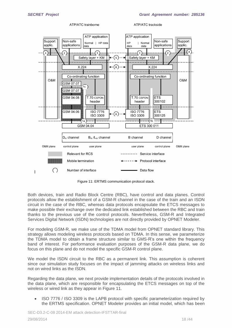
Figure 11: ERTMS communication protocol stack.

Both devices, train and Radio Block Centre (RBC), have control and data planes. Control protocols allow the establishment of a GSM-R channel in the case of the train and an ISDN circuit in the case of the RBC, whereas data protocols encapsulate the ETCS messages to make possible their exchange over the dedicated link established between the RBC and train thanks to the previous use of the control protocols. Nevertheless, GSM-R and Integrated Services Digital Network (ISDN) technologies are not directly provided by OPNET Modeler. For modeling GSM-R, we make use of the TDMA model from OPNET standard library. This strategy allows modeling wireless protocols based on TDMA. In this sense, we parameterize the TDMA model to obtain a frame structure similar to GMS-R’s one within the frequency band of interest. For performance evaluation purposes of the GSM-R data plane, we do focus on this plane and do not model the specific GSM-R control plane. We model the ISDN circuit to the RBC as a permanent link. This assumption is coherent since our simulation study focuses on the impact of jamming attacks on wireless links and not on wired links as the ISDN. Regarding the data plane, we next provide implementation details of the protocols involved in the data plane, which are responsible for encapsulating the ETCS messages on top of the wireless or wired link as they appear in Figure 11.

ISO 7776 / ISO 3309 is the LAPB protocol with specific parameterization required by the ERTMS specification. OPNET Modeler provides an initial model, which has been



29/08/2014 19 /44

modified to meet its requirements.

T.70 is a network protocol which is not included in the models supplied with OPNET. We entirely model it for this simulation study purposes.

X.224 is a transport protocol which is not included in the models supplied with OPNET. We entirely model it for this simulation study purposes.

Safety layer + KM layer is the Euroradio protocol used to establish safety connections between train and the RBC. This protocol is not supplied with the OPNET Modeler and, at this stage, we do not model it. It is worth pointing out that the objective of our simulation is to analyze the impact of EM attacks on the railway infrastructure. In order to analyze them, the lower protocols (LAPB, T.70 and X.224) are responsible for packet retransmission, segmentation and reassembly, which are the main operations that may be affected by a lossy or jammed wireless channel.

Automatic Train Protection (ATP) application exchanges ETCS messages between the train and the RBC and ensure safety in order to prevent collisions. We model entirely the ATP application for this simulation study purposes. The architecture of the ATP Application involves two different modules (train and RBC) and it is later detailed.

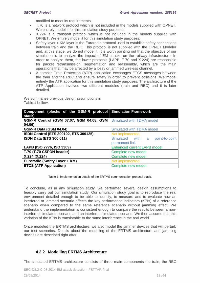
We summarize previous design assumptions in Table 1 bellow.

Component (blocks of the GSM-R protocol stack)

Simulation Framework

GSM-R Control (GSM 07.07, GSM 04.08, GSM 04.06)

Simulated with TDMA model

GSM-R Data (GSM 04.04) Simulated with TDMA model

ISDN Control (ETS 300102, ETS 300125) Not implemented

ISDN Data (ETS 300 011) Simulated with a point-to-point permanent link

LAPB (ISO 7776, ISO 3309) Enhanced current LAPB model

T.70 (T.70 CSPDN header) Complete new model

X.224 (X.224) Complete new model

Euroradio (Safety Layer + KM) Not implemented

ETCS (ATP Application) Complete new model

Table 1: Implementation details of the ERTMS communication protocol stack.

To conclude, as in any simulation study, we performed several design assumptions to feasibly carry out our simulation study. Our simulation study goal is to reproduce the real environment detailed enough to be able to identify, to measure and to evaluate how an interfered or jammed scenario affects the key performance indicators (KPIs) of a reference scenario when compared to the same reference scenario without jamming effect. We understand the implementation is consistent enough to compare the results between a non-interfered simulated scenario and an interfered simulated scenario. We then assume that this variation of the KPIs is translatable to the same interference in the real world. Once modeled the ERTMS architecture, we also model the jammer devices that will perturb our test scenarios. Details about the modeling of the ERTMS architecture and jamming devices are described right after.

4.2.2 Modelling ERTMS Architecture

The simulated ERTMS architecture consists of three main components the train, the RBC



29/08/2014 20 /44

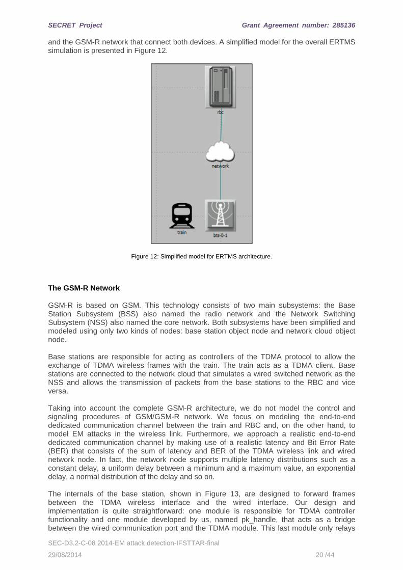
and the GSM-R network that connect both devices. A simplified model for the overall ERTMS simulation is presented in Figure 12.

Figure 12: Simplified model for ERTMS architecture.

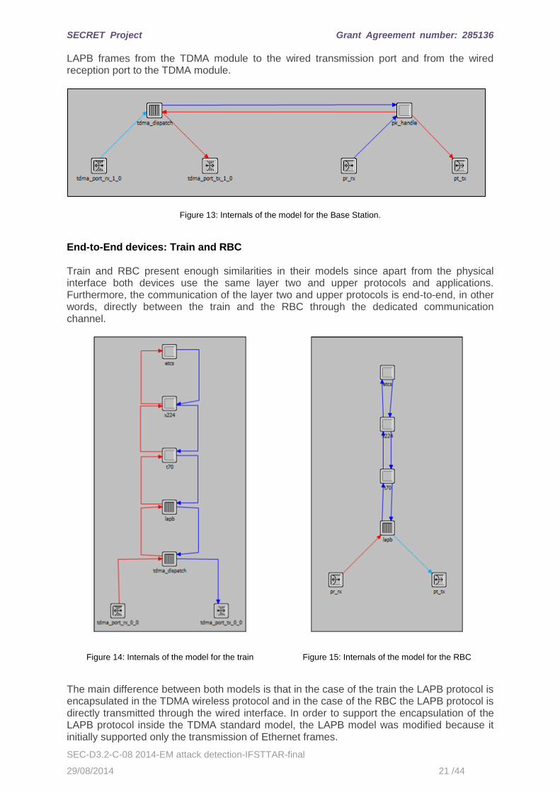
The GSM-R Network GSM-R is based on GSM. This technology consists of two main subsystems: the Base Station Subsystem (BSS) also named the radio network and the Network Switching Subsystem (NSS) also named the core network. Both subsystems have been simplified and modeled using only two kinds of nodes: base station object node and network cloud object node. Base stations are responsible for acting as controllers of the TDMA protocol to allow the exchange of TDMA wireless frames with the train. The train acts as a TDMA client. Base stations are connected to the network cloud that simulates a wired switched network as the NSS and allows the transmission of packets from the base stations to the RBC and vice versa. Taking into account the complete GSM-R architecture, we do not model the control and signaling procedures of GSM/GSM-R network. We focus on modeling the end-to-end dedicated communication channel between the train and RBC and, on the other hand, to model EM attacks in the wireless link. Furthermore, we approach a realistic end-to-end dedicated communication channel by making use of a realistic latency and Bit Error Rate (BER) that consists of the sum of latency and BER of the TDMA wireless link and wired network node. In fact, the network node supports multiple latency distributions such as a constant delay, a uniform delay between a minimum and a maximum value, an exponential delay, a normal distribution of the delay and so on. The internals of the base station, shown in Figure 13, are designed to forward frames between the TDMA wireless interface and the wired interface. Our design and implementation is quite straightforward: one module is responsible for TDMA controller functionality and one module developed by us, named pk_handle, that acts as a bridge between the wired communication port and the TDMA module. This last module only relays



29/08/2014 21 /44

LAPB frames from the TDMA module to the wired transmission port and from the wired reception port to the TDMA module.

Figure 13: Internals of the model for the Base Station.

End-to-End devices: Train and RBC Train and RBC present enough similarities in their models since apart from the physical interface both devices use the same layer two and upper protocols and applications. Furthermore, the communication of the layer two and upper protocols is end-to-end, in other words, directly between the train and the RBC through the dedicated communication channel.

Figure 14: Internals of the model for the train

Figure 15: Internals of the model for the RBC

The main difference between both models is that in the case of the train the LAPB protocol is encapsulated in the TDMA wireless protocol and in the case of the RBC the LAPB protocol is directly transmitted through the wired interface. In order to support the encapsulation of the LAPB protocol inside the TDMA standard model, the LAPB model was modified because it initially supported only the transmission of Ethernet frames.



29/08/2014 22 /44

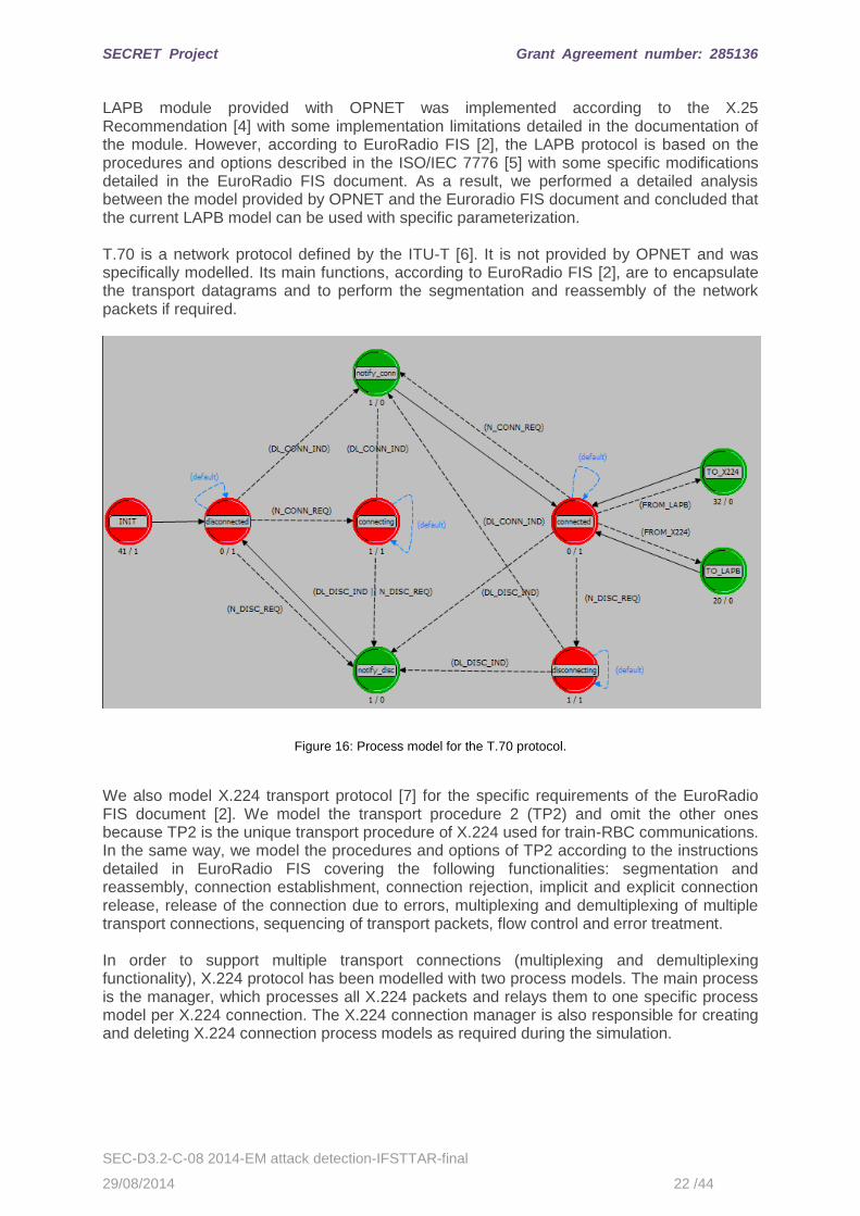
LAPB module provided with OPNET was implemented according to the X.25 Recommendation [4] with some implementation limitations detailed in the documentation of the module. However, according to EuroRadio FIS [2], the LAPB protocol is based on the procedures and options described in the ISO/IEC 7776 [5] with some specific modifications detailed in the EuroRadio FIS document. As a result, we performed a detailed analysis between the model provided by OPNET and the Euroradio FIS document and concluded that the current LAPB model can be used with specific parameterization. T.70 is a network protocol defined by the ITU-T [6]. It is not provided by OPNET and was specifically modelled. Its main functions, according to EuroRadio FIS [2], are to encapsulate the transport datagrams and to perform the segmentation and reassembly of the network packets if required.

Figure 16: Process model for the T.70 protocol.

We also model X.224 transport protocol [7] for the specific requirements of the EuroRadio FIS document [2]. We model the transport procedure 2 (TP2) and omit the other ones because TP2 is the unique transport procedure of X.224 used for train-RBC communications. In the same way, we model the procedures and options of TP2 according to the instructions detailed in EuroRadio FIS covering the following functionalities: segmentation and reassembly, connection establishment, connection rejection, implicit and explicit connection release, release of the connection due to errors, multiplexing and demultiplexing of multiple transport connections, sequencing of transport packets, flow control and error treatment. In order to support multiple transport connections (multiplexing and demultiplexing functionality), X.224 protocol has been modelled with two process models. The main process is the manager, which processes all X.224 packets and relays them to one specific process model per X.224 connection. The X.224 connection manager is also responsible for creating and deleting X.224 connection process models as required during the simulation.



29/08/2014 23 /44

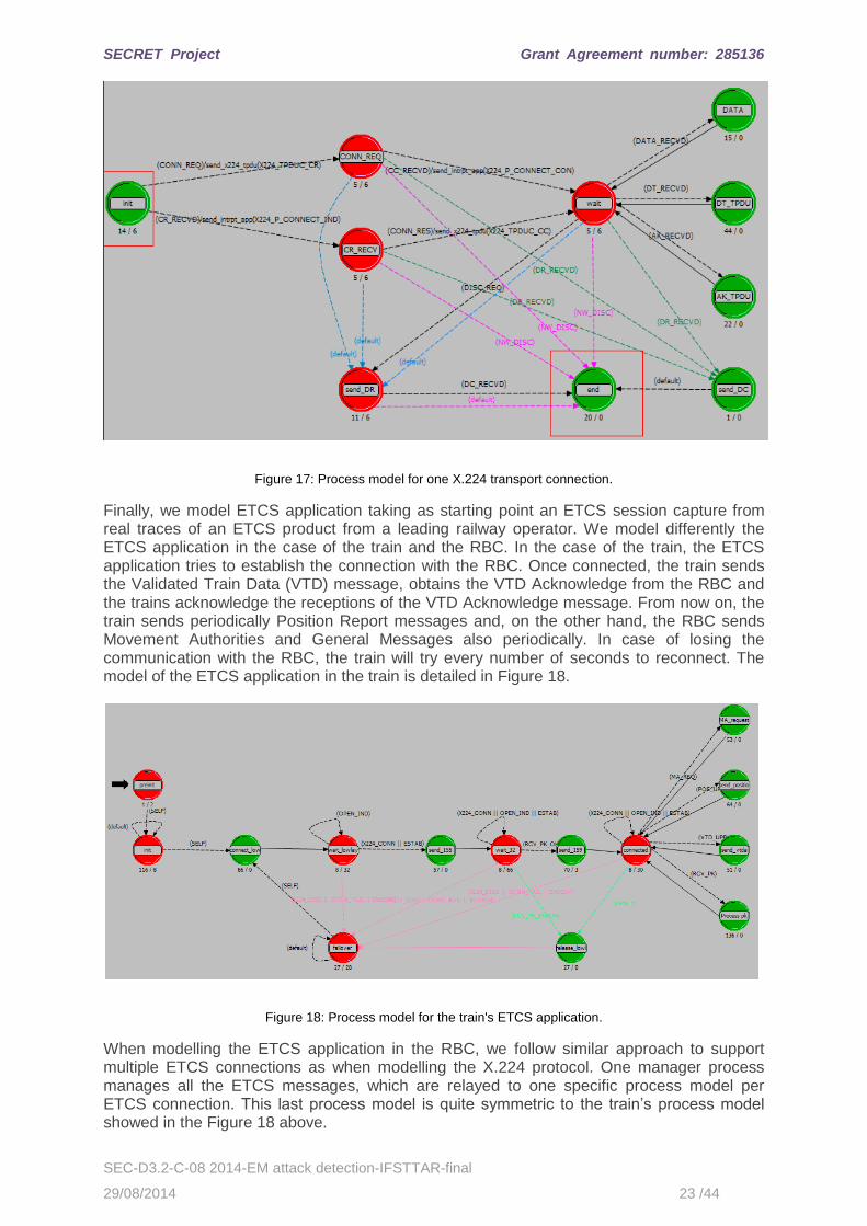
Figure 17: Process model for one X.224 transport connection.

Finally, we model ETCS application taking as starting point an ETCS session capture from real traces of an ETCS product from a leading railway operator. We model differently the ETCS application in the case of the train and the RBC. In the case of the train, the ETCS application tries to establish the connection with the RBC. Once connected, the train sends the Validated Train Data (VTD) message, obtains the VTD Acknowledge from the RBC and the trains acknowledge the receptions of the VTD Acknowledge message. From now on, the train sends periodically Position Report messages and, on the other hand, the RBC sends Movement Authorities and General Messages also periodically. In case of losing the communication with the RBC, the train will try every number of seconds to reconnect. The model of the ETCS application in the train is detailed in Figure 18.

Figure 18: Process model for the train's ETCS application.

When modelling the ETCS application in the RBC, we follow similar approach to support multiple ETCS connections as when modelling the X.224 protocol. One manager process manages all the ETCS messages, which are relayed to one specific process model per ETCS connection. This last process model is quite symmetric to the train’s process model showed in the Figure 18 above.



29/08/2014 24 /44

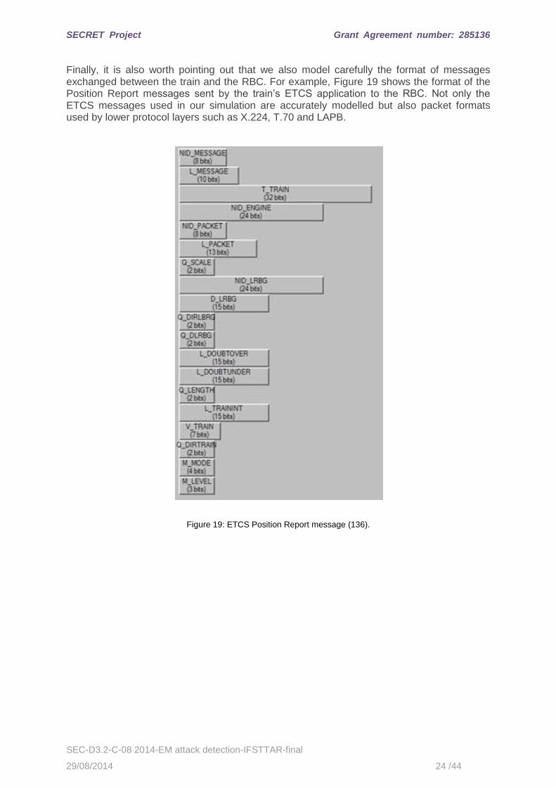
Finally, it is also worth pointing out that we also model carefully the format of messages exchanged between the train and the RBC. For example, Figure 19 shows the format of the Position Report messages sent by the train’s ETCS application to the RBC. Not only the ETCS messages used in our simulation are accurately modelled but also packet formats used by lower protocol layers such as X.224, T.70 and LAPB.

Figure 19: ETCS Position Report message (136).



29/08/2014 25 /44

4.2.3 Modelling attack devices

Work Package 3 considers two different jammers whose code names are silver jammer and grey jammer. Their jamming characteristics have been modelled in the simulation framework.

Figure 20: Jammer device.

First jammer: Silver Jammer The output of the grey jammer presented in the Figure 21 was measured on the 923 MHz channel with a 40 dB attenuator and a 120 kHz filter. However, these values are also representatives for all frequency bands of GSM-R affecting both, downlink and uplink frequency bands. Thus, the research team agreed on modelling the jammer as a continuous jammer with a constant output power of 10 dBm in the 840-976 MHz frequency band, since according to jamming lab test the difference between a steady continuous wave (CW) signal centred in the communication channel and a very fast sweeping signal is negligible.

Figure 21: Output of the silver jammer on the 923 MHz channel with a 40 dB attenuator and 120 kHz filter.

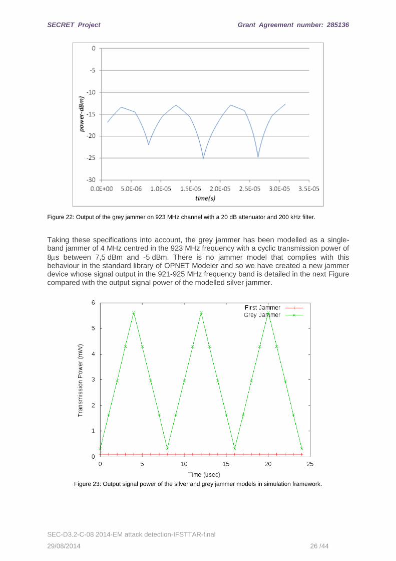
OPNET Modeller already supplies a continuous jammer model in the standard model library, which can be parameterized to change key parameters such as the frequency band and the output power. Second jammer: Grey Jammer The output of the second jammer, Figure 22, is measured centered on the same 923 MHz channel with a 20 dB attenuator and 200 kHz filter. This jammer provides a greater variety of the output signal with a frequency of 8 microseconds. The jammer presents a similar behaviour in the rest of the downlink channels of GSM-R and it does not affect the uplink channels.



29/08/2014 26 /44

Figure 22: Output of the grey jammer on 923 MHz channel with a 20 dB attenuator and 200 kHz filter.

Taking these specifications into account, the grey jammer has been modelled as a single-band jammer of 4 MHz centred in the 923 MHz frequency with a cyclic transmission power of

8s between 7,5 dBm and -5 dBm. There is no jammer model that complies with this behaviour in the standard library of OPNET Modeler and so we have created a new jammer device whose signal output in the 921-925 MHz frequency band is detailed in the next Figure compared with the output signal power of the modelled silver jammer.

Figure 23: Output signal power of the silver and grey jammer models in simulation framework.



29/08/2014 27 /44

4.3 Reference scenario

4.3.1 Definition of the reference scenario

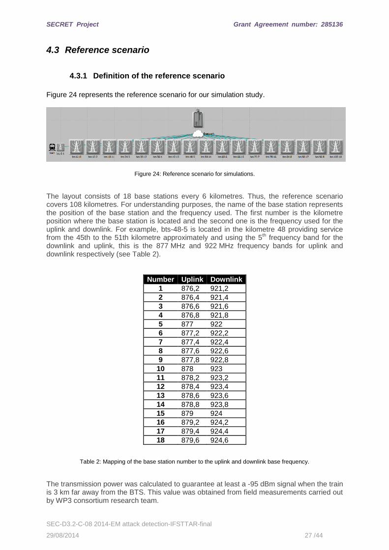
Figure 24 represents the reference scenario for our simulation study.

Figure 24: Reference scenario for simulations.

The layout consists of 18 base stations every 6 kilometres. Thus, the reference scenario covers 108 kilometres. For understanding purposes, the name of the base station represents the position of the base station and the frequency used. The first number is the kilometre position where the base station is located and the second one is the frequency used for the uplink and downlink. For example, bts-48-5 is located in the kilometre 48 providing service from the 45th to the 51th kilometre approximately and using the 5th frequency band for the downlink and uplink, this is the 877 MHz and 922 MHz frequency bands for uplink and downlink respectively (see Table 2).

Number Uplink Downlink

1 876,2 921,2

2 876,4 921,4

3 876,6 921,6

4 876,8 921,8

5 877 922

6 877,2 922,2

7 877,4 922,4

8 877,6 922,6

9 877,8 922,8

10 878 923

11 878,2 923,2

12 878,4 923,4

13 878,6 923,6

14 878,8 923,8

15 879 924

16 879,2 924,2

17 879,4 924,4

18 879,6 924,6

Table 2: Mapping of the base station number to the uplink and downlink base frequency.

The transmission power was calculated to guarantee at least a -95 dBm signal when the train is 3 km far away from the BTS. This value was obtained from field measurements carried out by WP3 consortium research team.



29/08/2014 28 /44

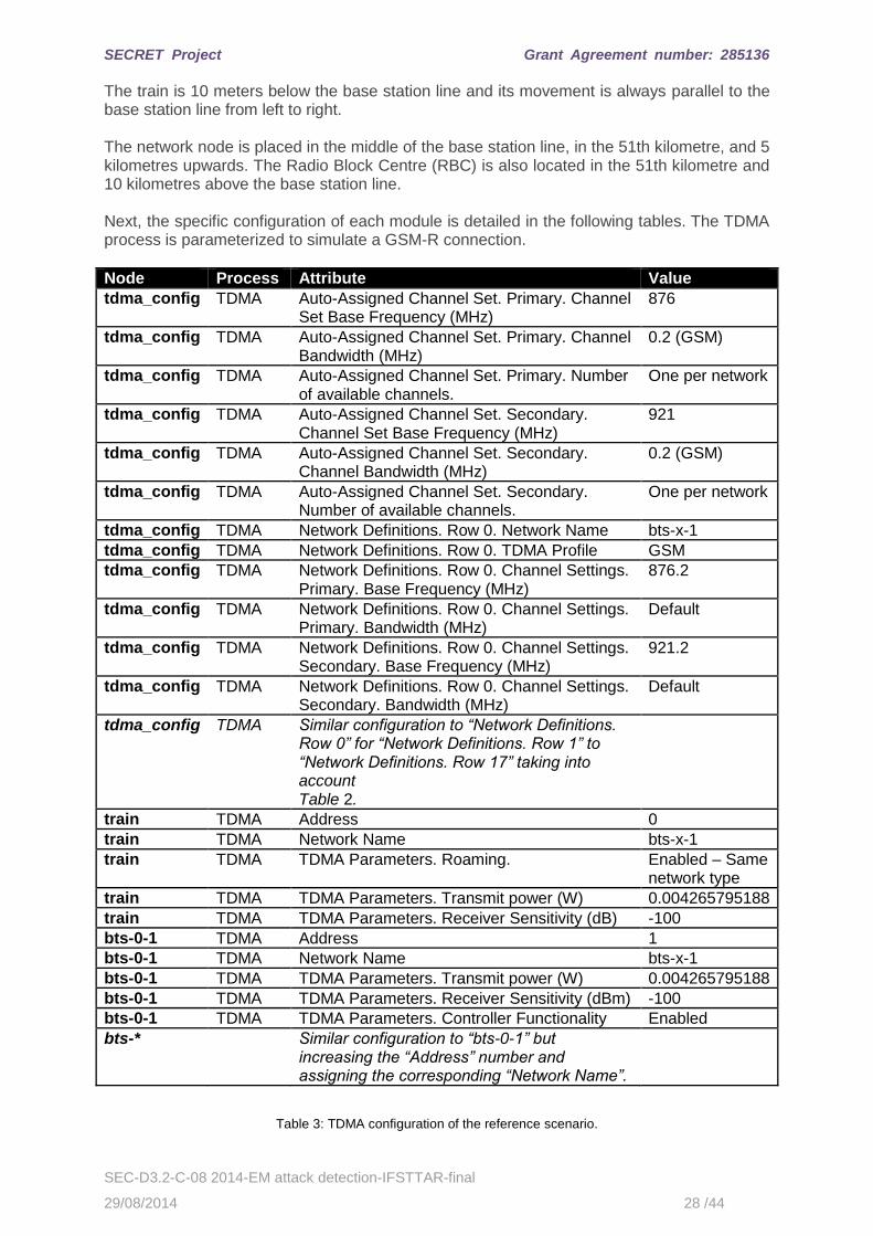
The train is 10 meters below the base station line and its movement is always parallel to the base station line from left to right. The network node is placed in the middle of the base station line, in the 51th kilometre, and 5 kilometres upwards. The Radio Block Centre (RBC) is also located in the 51th kilometre and 10 kilometres above the base station line. Next, the specific configuration of each module is detailed in the following tables. The TDMA process is parameterized to simulate a GSM-R connection.

Node Process Attribute Value

tdma_config TDMA Auto-Assigned Channel Set. Primary. Channel Set Base Frequency (MHz)

876

tdma_config TDMA Auto-Assigned Channel Set. Primary. Channel Bandwidth (MHz)

0.2 (GSM)

tdma_config TDMA Auto-Assigned Channel Set. Primary. Number of available channels.

One per network

tdma_config TDMA Auto-Assigned Channel Set. Secondary. Channel Set Base Frequency (MHz)

921

tdma_config TDMA Auto-Assigned Channel Set. Secondary. Channel Bandwidth (MHz)

0.2 (GSM)

tdma_config TDMA Auto-Assigned Channel Set. Secondary. Number of available channels.

One per network

tdma_config TDMA Network Definitions. Row 0. Network Name bts-x-1

tdma_config TDMA Network Definitions. Row 0. TDMA Profile GSM

tdma_config TDMA Network Definitions. Row 0. Channel Settings. Primary. Base Frequency (MHz)

876.2

tdma_config TDMA Network Definitions. Row 0. Channel Settings. Primary. Bandwidth (MHz)

Default

tdma_config TDMA Network Definitions. Row 0. Channel Settings. Secondary. Base Frequency (MHz)

921.2

tdma_config TDMA Network Definitions. Row 0. Channel Settings. Secondary. Bandwidth (MHz)

Default

tdma_config TDMA Similar configuration to “Network Definitions. Row 0” for “Network Definitions. Row 1” to “Network Definitions. Row 17” taking into account Table 2.

train TDMA Address 0

train TDMA Network Name bts-x-1

train TDMA TDMA Parameters. Roaming. Enabled – Same network type

train TDMA TDMA Parameters. Transmit power (W) 0.004265795188

train TDMA TDMA Parameters. Receiver Sensitivity (dB) -100

bts-0-1 TDMA Address 1

bts-0-1 TDMA Network Name bts-x-1

bts-0-1 TDMA TDMA Parameters. Transmit power (W) 0.004265795188

bts-0-1 TDMA TDMA Parameters. Receiver Sensitivity (dBm) -100

bts-0-1 TDMA TDMA Parameters. Controller Functionality Enabled

bts-* Similar configuration to “bts-0-1” but increasing the “Address” number and assigning the corresponding “Network Name”.

Table 3: TDMA configuration of the reference scenario.



29/08/2014 29 /44

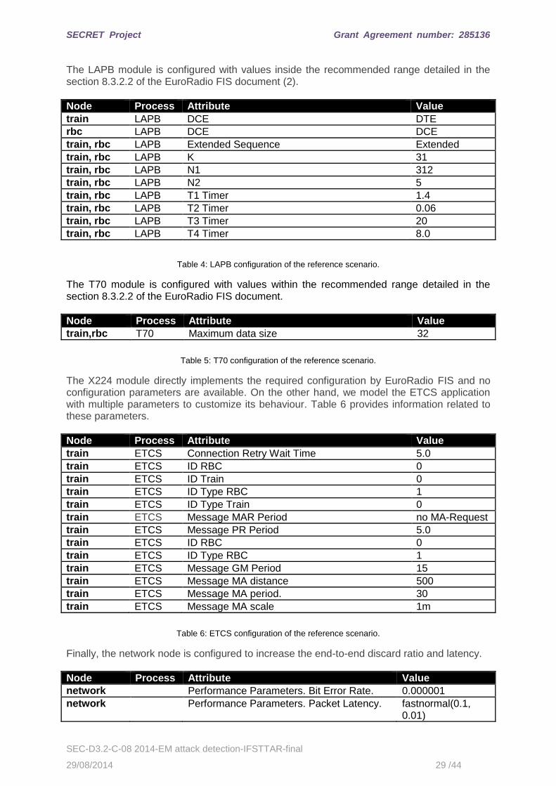
The LAPB module is configured with values inside the recommended range detailed in the section 8.3.2.2 of the EuroRadio FIS document (2).


train LAPB DCE DTE

rbc LAPB DCE DCE

train, rbc LAPB Extended Sequence Extended

train, rbc LAPB K 31

train, rbc LAPB N1 312

train, rbc LAPB N2 5

train, rbc LAPB T1 Timer 1.4


train, rbc LAPB T3 Timer 20


Table 4: LAPB configuration of the reference scenario.

The T70 module is configured with values within the recommended range detailed in the section 8.3.2.2 of the EuroRadio FIS document.


train,rbc T70 Maximum data size 32

Table 5: T70 configuration of the reference scenario.

The X224 module directly implements the required configuration by EuroRadio FIS and no configuration parameters are available. On the other hand, we model the ETCS application with multiple parameters to customize its behaviour. Table 6 provides information related to these parameters.


train ETCS Connection Retry Wait Time 5.0

train ETCS ID RBC 0

train ETCS ID Train 0

train ETCS ID Type RBC 1

train ETCS ID Type Train 0

train ETCS Message MAR Period no MA-Request

train ETCS Message PR Period 5.0

train ETCS ID RBC 0

train ETCS ID Type RBC 1

train ETCS Message GM Period 15

train ETCS Message MA distance 500

train ETCS Message MA period. 30

train ETCS Message MA scale 1m

Table 6: ETCS configuration of the reference scenario.

Finally, the network node is configured to increase the end-to-end discard ratio and latency.


network Performance Parameters. Bit Error Rate. 0.000001

network Performance Parameters. Packet Latency. fastnormal(0.1, 0.01)



29/08/2014 30 /44

Table 7: Network node configuration of the reference scenario.

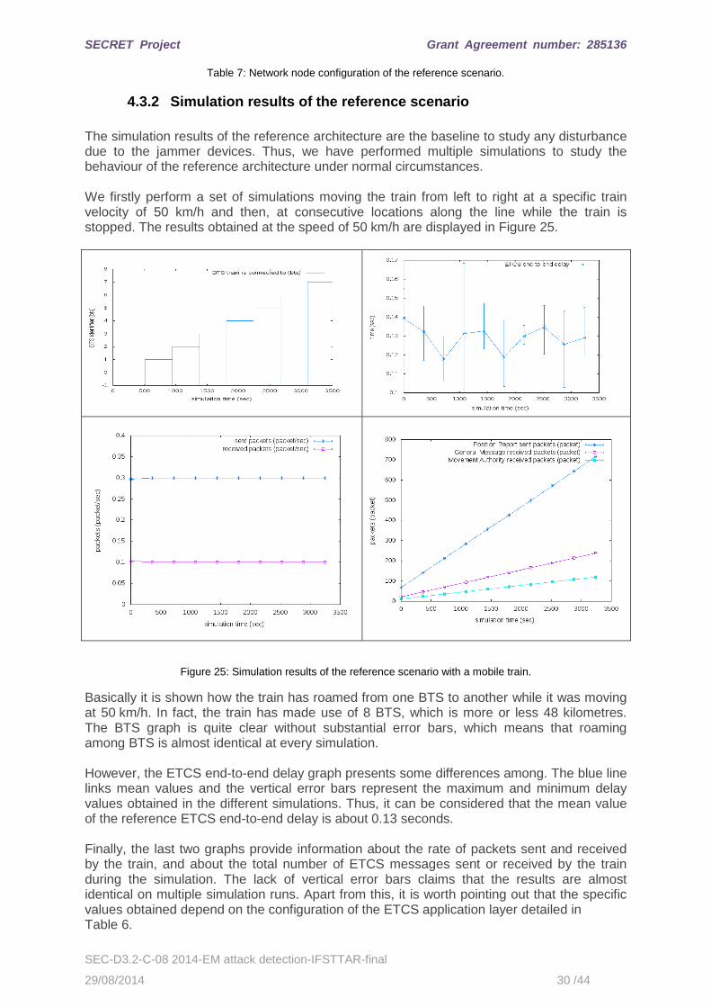
4.3.2 Simulation results of the reference scenario

The simulation results of the reference architecture are the baseline to study any disturbance due to the jammer devices. Thus, we have performed multiple simulations to study the behaviour of the reference architecture under normal circumstances. We firstly perform a set of simulations moving the train from left to right at a specific train velocity of 50 km/h and then, at consecutive locations along the line while the train is stopped. The results obtained at the speed of 50 km/h are displayed in Figure 25.

Figure 25: Simulation results of the reference scenario with a mobile train.

Basically it is shown how the train has roamed from one BTS to another while it was moving at 50 km/h. In fact, the train has made use of 8 BTS, which is more or less 48 kilometres. The BTS graph is quite clear without substantial error bars, which means that roaming among BTS is almost identical at every simulation. However, the ETCS end-to-end delay graph presents some differences among. The blue line links mean values and the vertical error bars represent the maximum and minimum delay values obtained in the different simulations. Thus, it can be considered that the mean value of the reference ETCS end-to-end delay is about 0.13 seconds. Finally, the last two graphs provide information about the rate of packets sent and received by the train, and about the total number of ETCS messages sent or received by the train during the simulation. The lack of vertical error bars claims that the results are almost identical on multiple simulation runs. Apart from this, it is worth pointing out that the specific values obtained depend on the configuration of the ETCS application layer detailed in Table 6.



29/08/2014 31 /44

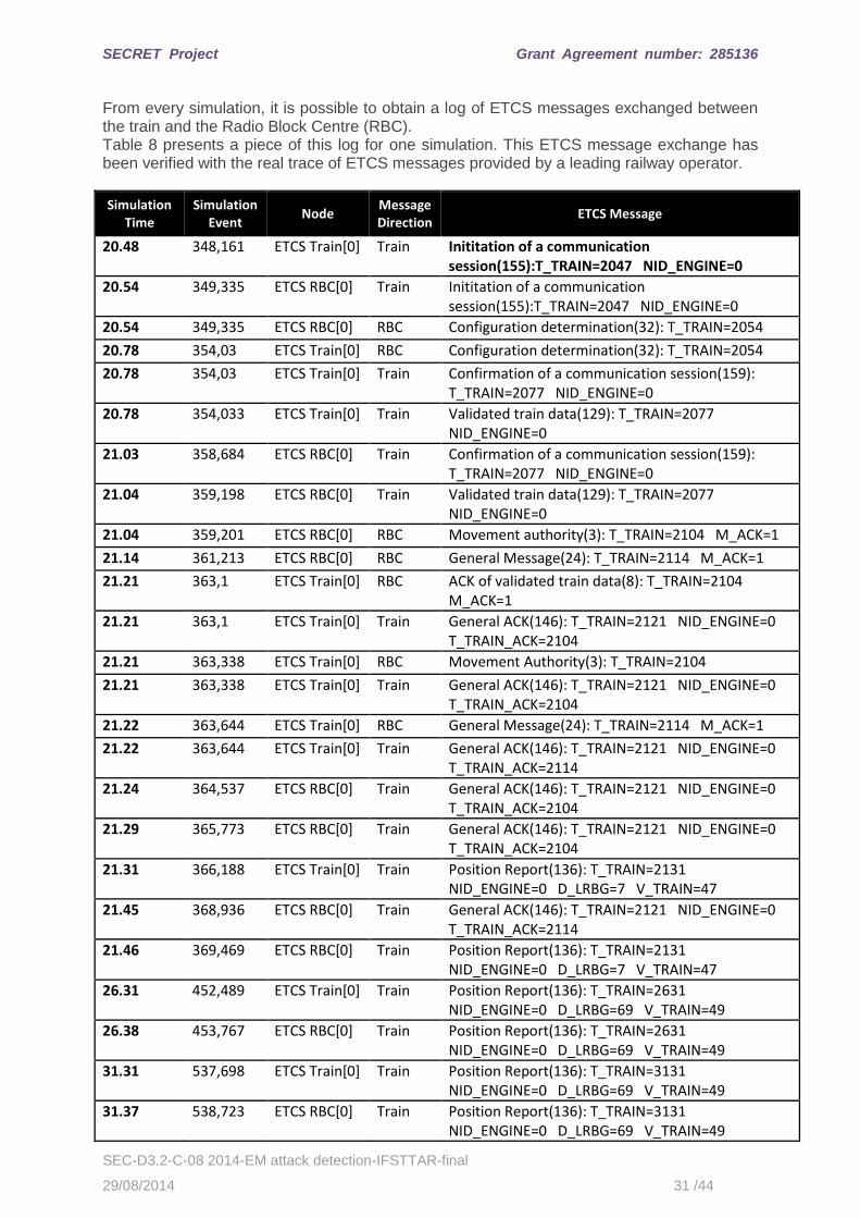
From every simulation, it is possible to obtain a log of ETCS messages exchanged between the train and the Radio Block Centre (RBC). Table 8 presents a piece of this log for one simulation. This ETCS message exchange has been verified with the real trace of ETCS messages provided by a leading railway operator.

Simulation Time

Simulation Event

Node Message Direction

ETCS Message

20.48 348,161 ETCS Train[0] Train Inititation of a communication session(155):T_TRAIN=2047 NID_ENGINE=0

20.54 349,335 ETCS RBC[0] Train Inititation of a communication session(155):T_TRAIN=2047 NID_ENGINE=0

20.54 349,335 ETCS RBC[0] RBC Configuration determination(32): T_TRAIN=2054

20.78 354,03 ETCS Train[0] RBC Configuration determination(32): T_TRAIN=2054

20.78 354,03 ETCS Train[0] Train Confirmation of a communication session(159): T_TRAIN=2077 NID_ENGINE=0

20.78 354,033 ETCS Train[0] Train Validated train data(129): T_TRAIN=2077 NID_ENGINE=0

21.03 358,684 ETCS RBC[0] Train Confirmation of a communication session(159): T_TRAIN=2077 NID_ENGINE=0

21.04 359,198 ETCS RBC[0] Train Validated train data(129): T_TRAIN=2077 NID_ENGINE=0

21.04 359,201 ETCS RBC[0] RBC Movement authority(3): T_TRAIN=2104 M_ACK=1

21.14 361,213 ETCS RBC[0] RBC General Message(24): T_TRAIN=2114 M_ACK=1

21.21 363,1 ETCS Train[0] RBC ACK of validated train data(8): T_TRAIN=2104 M_ACK=1

21.21 363,1 ETCS Train[0] Train General ACK(146): T_TRAIN=2121 NID_ENGINE=0 T_TRAIN_ACK=2104

21.21 363,338 ETCS Train[0] RBC Movement Authority(3): T_TRAIN=2104


21.22 363,644 ETCS Train[0] RBC General Message(24): T_TRAIN=2114 M_ACK=1


21.24 364,537 ETCS RBC[0] Train General ACK(146): T_TRAIN=2121 NID_ENGINE=0 T_TRAIN_ACK=2104


21.31 366,188 ETCS Train[0] Train Position Report(136): T_TRAIN=2131 NID_ENGINE=0 D_LRBG=7 V_TRAIN=47


21.46 369,469 ETCS RBC[0] Train Position Report(136): T_TRAIN=2131 NID_ENGINE=0 D_LRBG=7 V_TRAIN=47







29/08/2014 32 /44

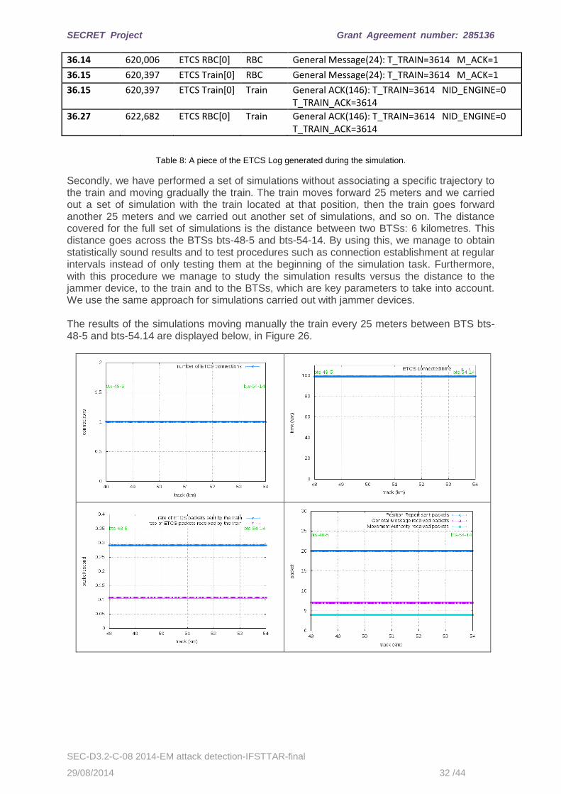
36.14 620,006 ETCS RBC[0] RBC General Message(24): T_TRAIN=3614 M_ACK=1

36.15 620,397 ETCS Train[0] RBC General Message(24): T_TRAIN=3614 M_ACK=1



Table 8: A piece of the ETCS Log generated during the simulation.

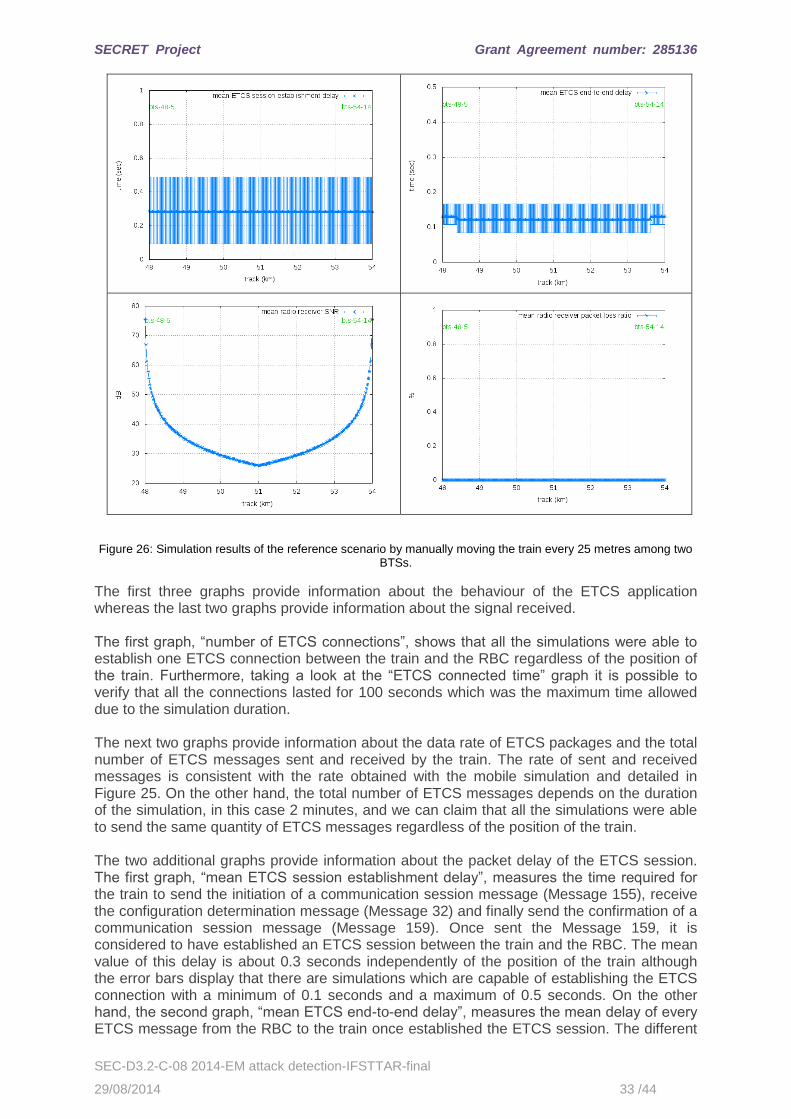
Secondly, we have performed a set of simulations without associating a specific trajectory to the train and moving gradually the train. The train moves forward 25 meters and we carried out a set of simulation with the train located at that position, then the train goes forward another 25 meters and we carried out another set of simulations, and so on. The distance covered for the full set of simulations is the distance between two BTSs: 6 kilometres. This distance goes across the BTSs bts-48-5 and bts-54-14. By using this, we manage to obtain statistically sound results and to test procedures such as connection establishment at regular intervals instead of only testing them at the beginning of the simulation task. Furthermore, with this procedure we manage to study the simulation results versus the distance to the jammer device, to the train and to the BTSs, which are key parameters to take into account. We use the same approach for simulations carried out with jammer devices. The results of the simulations moving manually the train every 25 meters between BTS bts-48-5 and bts-54.14 are displayed below, in Figure 26.



29/08/2014 33 /44

Figure 26: Simulation results of the reference scenario by manually moving the train every 25 metres among two BTSs.

The first three graphs provide information about the behaviour of the ETCS application whereas the last two graphs provide information about the signal received. The first graph, “number of ETCS connections”, shows that all the simulations were able to establish one ETCS connection between the train and the RBC regardless of the position of the train. Furthermore, taking a look at the “ETCS connected time” graph it is possible to verify that all the connections lasted for 100 seconds which was the maximum time allowed due to the simulation duration. The next two graphs provide information about the data rate of ETCS packages and the total number of ETCS messages sent and received by the train. The rate of sent and received messages is consistent with the rate obtained with the mobile simulation and detailed in Figure 25. On the other hand, the total number of ETCS messages depends on the duration of the simulation, in this case 2 minutes, and we can claim that all the simulations were able to send the same quantity of ETCS messages regardless of the position of the train. The two additional graphs provide information about the packet delay of the ETCS session. The first graph, “mean ETCS session establishment delay”, measures the time required for the train to send the initiation of a communication session message (Message 155), receive the configuration determination message (Message 32) and finally send the confirmation of a communication session message (Message 159). Once sent the Message 159, it is considered to have established an ETCS session between the train and the RBC. The mean value of this delay is about 0.3 seconds independently of the position of the train although the error bars display that there are simulations which are capable of establishing the ETCS connection with a minimum of 0.1 seconds and a maximum of 0.5 seconds. On the other hand, the second graph, “mean ETCS end-to-end delay”, measures the mean delay of every ETCS message from the RBC to the train once established the ETCS session. The different



29/08/2014 34 /44

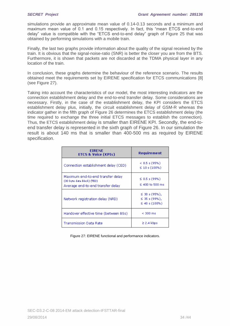
simulations provide an approximate mean value of 0.14-0.13 seconds and a minimum and maximum mean value of 0.1 and 0.15 respectively. In fact, this “mean ETCS end-to-end delay” value is compatible with the “ETCS end-to-end delay” graph of Figure 25 that was obtained by performing simulations with a mobile train. Finally, the last two graphs provide information about the quality of the signal received by the train. It is obvious that the signal-noise-ratio (SNR) is better the closer you are from the BTS. Furthermore, it is shown that packets are not discarded at the TDMA physical layer in any location of the train. In conclusion, these graphs determine the behaviour of the reference scenario. The results obtained meet the requirements set by EIRENE specification for ETCS communications [8] (see Figure 27). Taking into account the characteristics of our model, the most interesting indicators are the connection establishment delay and the end-to-end transfer delay. Some considerations are necessary. Firstly, in the case of the establishment delay, the KPI considers the ETCS establishment delay plus, initially, the circuit establishment delay of GSM-R whereas the indicator gather in the fifth graph of Figure 26 determines the ETCS establishment delay (the time required to exchange the three initial ETCS messages to establish the connection).

Thus, the ETCS establishment delay is smaller than EIRENE KPI. Secondly, the end-to-end transfer delay is represented in the sixth graph of Figure 26. In our simulation the result is about 140 ms that is smaller than 400-500 ms as required by EIRENE specification.

Figure 27: EIRENE functional and performance indicators.



29/08/2014 35 /44

4.4 Interfered scenarios

4.4.1 Silver Jammer

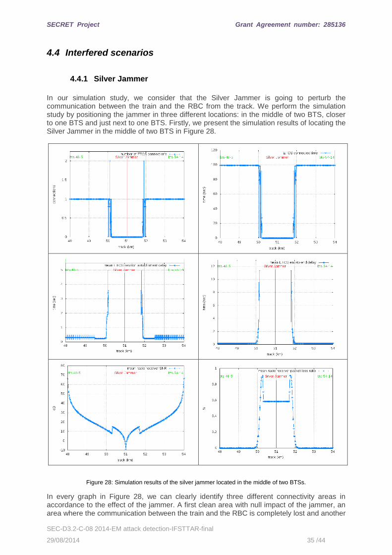
In our simulation study, we consider that the Silver Jammer is going to perturb the communication between the train and the RBC from the track. We perform the simulation study by positioning the jammer in three different locations: in the middle of two BTS, closer to one BTS and just next to one BTS. Firstly, we present the simulation results of locating the Silver Jammer in the middle of two BTS in Figure 28.

Figure 28: Simulation results of the silver jammer located in the middle of two BTSs.

In every graph in Figure 28, we can clearly identify three different connectivity areas in accordance to the effect of the jammer. A first clean area with null impact of the jammer, an area where the communication between the train and the RBC is completely lost and another



29/08/2014 36 /44

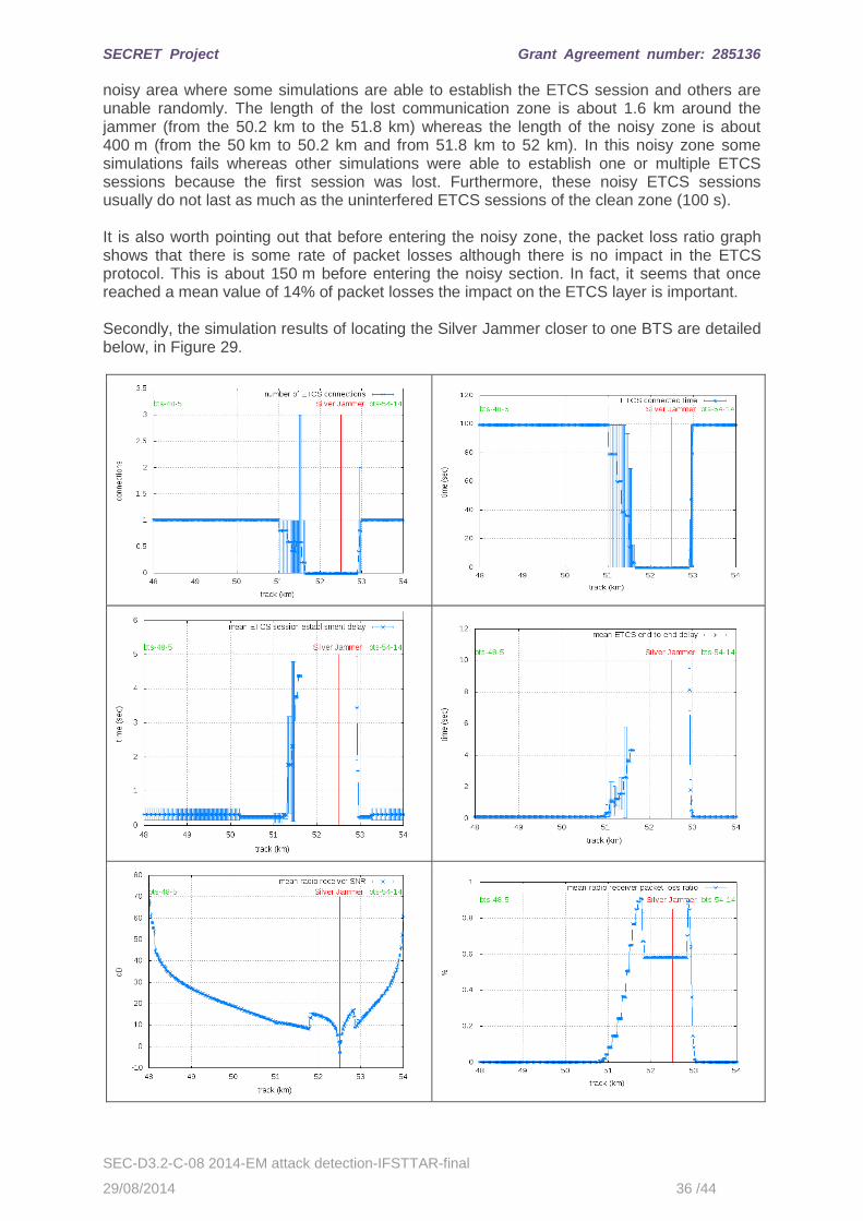
noisy area where some simulations are able to establish the ETCS session and others are unable randomly. The length of the lost communication zone is about 1.6 km around the jammer (from the 50.2 km to the 51.8 km) whereas the length of the noisy zone is about 400 m (from the 50 km to 50.2 km and from 51.8 km to 52 km). In this noisy zone some simulations fails whereas other simulations were able to establish one or multiple ETCS sessions because the first session was lost. Furthermore, these noisy ETCS sessions usually do not last as much as the uninterfered ETCS sessions of the clean zone (100 s). It is also worth pointing out that before entering the noisy zone, the packet loss ratio graph shows that there is some rate of packet losses although there is no impact in the ETCS protocol. This is about 150 m before entering the noisy section. In fact, it seems that once reached a mean value of 14% of packet losses the impact on the ETCS layer is important. Secondly, the simulation results of locating the Silver Jammer closer to one BTS are detailed below, in Figure 29.



29/08/2014 37 /44

Figure 29: Simulation results of the silver jammer located closer to one BTS.

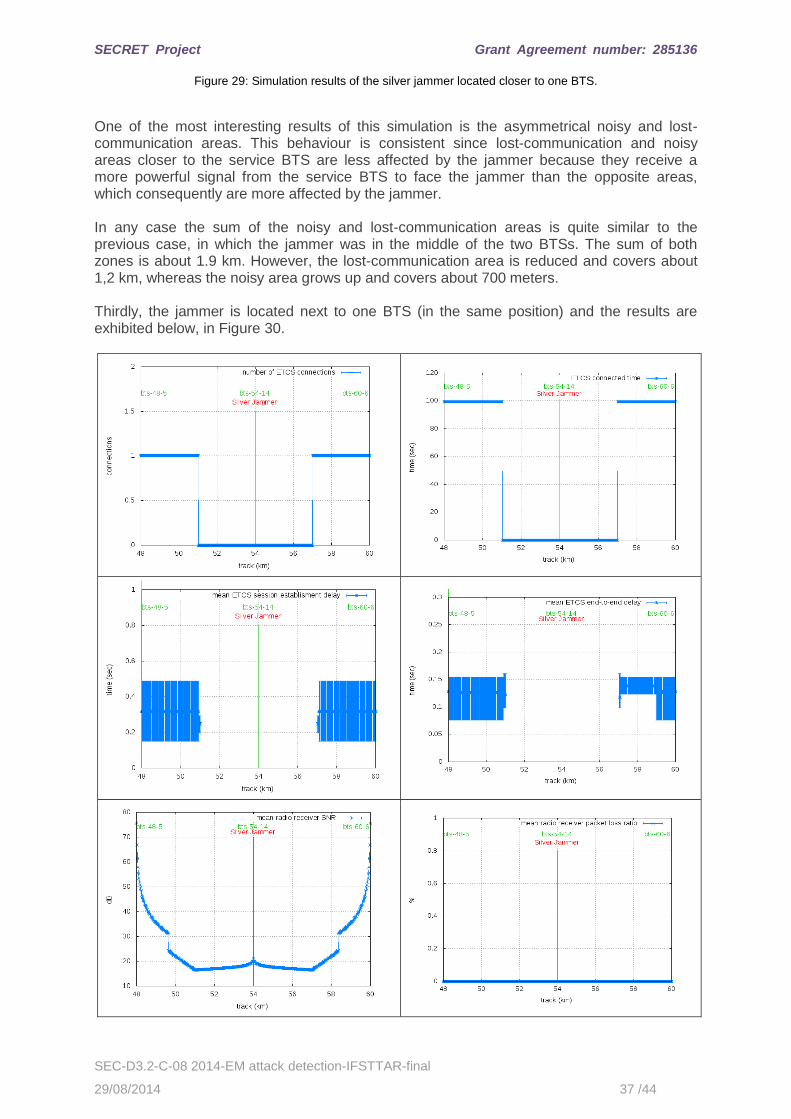
One of the most interesting results of this simulation is the asymmetrical noisy and lost-communication areas. This behaviour is consistent since lost-communication and noisy areas closer to the service BTS are less affected by the jammer because they receive a more powerful signal from the service BTS to face the jammer than the opposite areas, which consequently are more affected by the jammer. In any case the sum of the noisy and lost-communication areas is quite similar to the previous case, in which the jammer was in the middle of the two BTSs. The sum of both zones is about 1.9 km. However, the lost-communication area is reduced and covers about 1,2 km, whereas the noisy area grows up and covers about 700 meters. Thirdly, the jammer is located next to one BTS (in the same position) and the results are exhibited below, in Figure 30.



29/08/2014 38 /44

Figure 30: Simulation results of the silver jammer located next to one BTS.

The results prove that the train cannot make use of the bts-54-14 along the 6 km that this BTS provides coverage. However, the SNR received by the train is not so bad and there are no packet losses according to the last graph of Figure 30. Thus, the loss of communication is not because the jammer is disturbing the train but mainly because Silver Jammer is disturbing directly the BTS bts-54-14 since this jammer not only jams the downlink channel but also the uplink channel. Figure 31 shows the SNR in the BTSs and how the jammer is affecting the bts-54-14 and causing a high packet loss ratio in all the coverage area of the bts-54-14 because even when the train is close to the bts-54-14, the jammer is closer and it is powerful enough to completely disturb the GSM signal.

Figure 31: Simulation results of the silver jammer located next to one BTS. Effect of the jammer on the BTSs.

The usage of the Silver Jammer close to one BTS is the worst scenario causing the largest lost communication zone along the 6 km of coverage of the specific BTS. Finally, in order to conclude the study of the silver jammer we considered different transmission powers up to 30 dBm. As it is shown in Figure 32, a 30 dBm Silver Jammer located in the middle of two BTSs is able to block almost the 6 km between the two BTSs.

Figure 32: Silver Jammer with different transmission powers located in the middle of two BTSs.



29/08/2014 39 /44

4.4.2 Grey Jammer

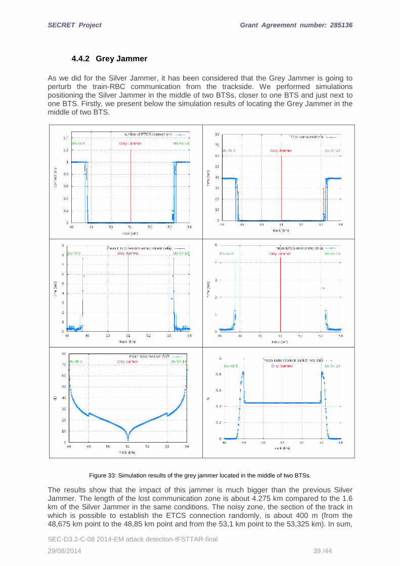
As we did for the Silver Jammer, it has been considered that the Grey Jammer is going to perturb the train-RBC communication from the trackside. We performed simulations positioning the Silver Jammer in the middle of two BTSs, closer to one BTS and just next to one BTS. Firstly, we present below the simulation results of locating the Grey Jammer in the middle of two BTS.

Figure 33: Simulation results of the grey jammer located in the middle of two BTSs.

The results show that the impact of this jammer is much bigger than the previous Silver Jammer. The length of the lost communication zone is about 4.275 km compared to the 1.6 km of the Silver Jammer in the same conditions. The noisy zone, the section of the track in which is possible to establish the ETCS connection randomly, is about 400 m (from the 48,675 km point to the 48,85 km point and from the 53,1 km point to the 53,325 km). In sum,



29/08/2014 40 /44

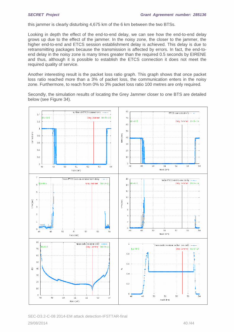
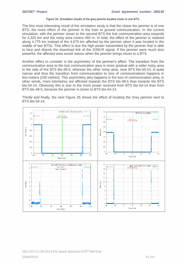
this jammer is clearly disturbing 4,675 km of the 6 km between the two BTSs. Looking in depth the effect of the end-to-end delay, we can see how the end-to-end delay grows up due to the effect of the jammer. In the noisy zone, the closer to the jammer, the higher end-to-end and ETCS session establishment delay is achieved. This delay is due to retransmitting packages because the transmission is affected by errors. In fact, the end-to-end delay in the noisy zone is many times greater than the required 0.5 seconds by EIRENE and thus, although it is possible to establish the ETCS connection it does not meet the required quality of service. Another interesting result is the packet loss ratio graph. This graph shows that once packet loss ratio reached more than a 3% of packet loss, the communication enters in the noisy zone. Furthermore, to reach from 0% to 3% packet loss ratio 100 metres are only required. Secondly, the simulation results of locating the Grey Jammer closer to one BTS are detailed below (see Figure 34).



29/08/2014 41 /44

Figure 34: Simulation results of the grey jammer located closer to one BTS.

The first most interesting result of the simulation study is that the closer the jammer is of one BTS, the more effect of the jammer in the train to ground communication. In the current simulation, with the jammer closer to the second BTS the lost communication area expands for 4,325 km and the noisy area covers 450 m. In total, the effect of the jammer is realized along 4,775 km instead of the 4,675 km affected by the jammer when it was located in the middle of two BTSs. This effect is due the high power transmitted by the jammer that is able to face and disturb the download link of the GSM-R signal. If the jammer were much less powerful, the affected area would reduce when the jammer brings closer to a BTS. Another effect to consider is the asymmetry of the jammer’s effect. The transition from the communication area to the lost communication area is more gradual with a wider noisy area in the side of the BTS bts-48-5, whereas the other noisy area, near BTS bts-54-14, is quite narrow and thus the transition from communication to loss of communications happens in few meters (100 metres). This asymmetry also happens in the loss of communication area, in other words, more kilometres are affected towards the BTS bts-48-5 than towards the BTS bts-54-14. Obviously this is due to the more power received from BTS bts-54-14 than from BTS bts-48-5, because the jammer is closer to BTS bts-54-14. Thirdly and finally, the next Figure 35 shows the effect of locating the Grey jammer next to BTS bts-54-14.



29/08/2014 42 /44

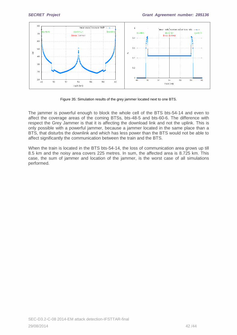
Figure 35: Simulation results of the grey jammer located next to one BTS.

The jammer is powerful enough to block the whole cell of the BTS bts-54-14 and even to affect the coverage areas of the coming BTSs, bts-48-5 and bts-60-6. The difference with respect the Grey Jammer is that it is affecting the download link and not the uplink. This is only possible with a powerful jammer, because a jammer located in the same place than a BTS, that disturbs the downlink and which has less power than the BTS would not be able to affect significantly the communication between the train and the BTS. When the train is located in the BTS bts-54-14, the loss of communication area grows up till 8.5 km and the noisy area covers 225 metres. In sum, the affected area is 8.725 km. This case, the sum of jammer and location of the jammer, is the worst case of all simulations performed.



29/08/2014 43 /44

5. Conclusion

This deliverable has described the results obtains in WP3, task 3.2 (a and b). We have presented different solutions to detect the presence of jamming signals. We described the quantities which can be monitored and the respective required measurement equipment. We have highlighted the advantages and disadvantages of these different approaches. On the one hand, the detection based on the analyses of the IQ data permit to monitor only the jamming of an unique communication system. However, it can permit to react very quickly and to avoid an unwanted automatic reaction and cause unnecessary inconvenience on the rail network. On the other, the detection solutions based on statistical analysis of the frequency spectrum and on the time characteristic can permit to monitor jamming signal able to affect different communication systems. These solutions can then be very useful in train stations where several communication systems are employed for operational application. The time of detection of these solutions is slower, but the delay of detection is not critical in this situation because there is no risk that an emergency brake being activated. In the simulation study, we evaluated, in terms of key performance indicators (KPIs) such as packet loss rates, end-to-end delays, connection establishment delays, signal to noise ratios and so on, the performance of an attacked or interfered railway communication architecture. We take as an input the jammer identified in previous WPs and we model these attack devices and their behaviour in the simulation platform. We also dedicate an important effort in developing in the simulation platform a reference ERTMS communication architecture (full legacy protocol stack plus a validated ETCS service). We perform a complete set of simulation runs modifying the location of the two types of jammer devices (the silver and grey jammers) and verify that the jammer devices under study disturb the upper layers and the ETCS quality of service indicators. We clearly identify three different zones or areas of behaviour: the clean zone, the noisy zone and the totally disturbed zone where no ETCS connectivity is possible. We identify also that the extension of these three zones is clearly dependant on the location of the jammer and most specifically on the distance of the jammer to the BTS. We also provide the relation between the transmission power of a Silver Jammer located in the middle of two BTSs and a higher KPI indicator such as the number of ETCS connections. Last but not least, the results also allow identifying an area where the ETCS connection exists nevertheless the quality of service for the KPIs, in accordance to EIRENE specification, is not achieved, this way allowing a pre-emptive functionality.



29/08/2014 44 /44

6. References

[1] Mili, S. ; Sodoyer, D. ; Deniau, V. ; Heddebaut, M. ; Philippe, H. ; Canavero, F., Recognition

process of jamming signals superimposed on GSM-R radiocommunications, International Symposium on Electromagnetic Compatibility (EMC EUROPE), 2013, pp45-50

[2] UNISIG. EuroRadio FIS. s.l. : ERTMS, 2013. Mandatory Specification. UNISIG SUBSET-037 (v3.0.0).

[3] Riverbed. SteelCentral for Performance Management and Control | Riverbed. [En línea] http://www.riverbed.com/products/performance-management-control/.

[4] ITU-T. Interface between Data Terminal Equipment (DTE) and Data Circuit-terminating

Equipment (DCE) for terminals operating in the packet mode and connected to public data networks by dedicated circuit. s.l. : ITU-T, 1996. ITU-T Recommendation X.25 (10/96).

[5] ISO. Information technology - Telecommunications and information exchange between systems -

High-level data link control procedures - Description of the X.25 LAPB-compatible DTE data link procedures . s.l. : ISO, 1995. ISO/IEC 7776.

[6] ITU-T. Network-independent basic transport service for the telematic services. s.l. : ITU-T, 1993.

ITU-T Recommendation T.70 (03/93).

[7] Information technology - Open Systems Interconnection - Protocol for providing the connection-

mode transport service. s.l. : ITU-T, 1995. ITU-T Recommendation X.224 (11/95).

[8] QoS Working Group. ERTMS/GSM-R QoS Test Specification. s.l. : ERTMS, 2013. O_2475

(v3.0).

http://ieeexplore.ieee.org/search/searchresult.jsp?searchWithin=p_Authors:.QT.Mili,%20S..QT.&newsearch=true

http://ieeexplore.ieee.org/search/searchresult.jsp?searchWithin=p_Authors:.QT.Sodoyer,%20D..QT.&newsearch=true

http://ieeexplore.ieee.org/search/searchresult.jsp?searchWithin=p_Authors:.QT.Deniau,%20V..QT.&newsearch=true

http://ieeexplore.ieee.org/search/searchresult.jsp?searchWithin=p_Authors:.QT.Heddebaut,%20M..QT.&newsearch=true

http://ieeexplore.ieee.org/search/searchresult.jsp?searchWithin=p_Authors:.QT.Philippe,%20H..QT.&newsearch=true

http://ieeexplore.ieee.org/search/searchresult.jsp?searchWithin=p_Authors:.QT.Canavero,%20F..QT.&newsearch=true

http://ieeexplore.ieee.org/xpl/mostRecentIssue.jsp?punumber=6636283

http://ieeexplore.ieee.org/xpl/mostRecentIssue.jsp?punumber=6636283

Documents

SECRET SECurity of Railways against Electromagnetic … · SECurity of Railways against Electromagnetic aTtacks ... 4.3.2 Simulation results of the reference scenario 30 ... KPI Key