Embed Size (px)
Citation preview

Secondary Sonic Boom
�Katerina Kaouri
Somerville College
University of Oxford
A thesis submitted for the degree of
Doctor of Philosophy
Trinity Term 2004

To my sister Marina for who she is.

Acknowledgements
The first place in these acknowledgements belongs to my supervisor Dr David
Allwright for all the help and support he has given me throughout the years. He
has guided me flawlessly and has always been available to answer all my questions
and correct my mistakes with immense clarity, speed and politeness. I am sure that
reading my thesis repeatedly was not a fun thing to do, but he did it diligently and
efficiently. Furthermore, David and his wife Susan have been very understanding and
helpful through difficult personal times; I am grateful for this.
I would also like to thank Dr John Ockendon for the many discussions on sonic
boom over the years, and for demonstrating the value of “solving the simplest prob-
lem first”. His input has been very valuable throughout the course of this work, in
particular for the asymptotic methods that were used in this thesis. I would also like
to gratefully acknowledge Dr Hilary Ockendon for being a very helpful and efficient
College Advisor throughout the years I spent in Oxford.
My friends Angelos, Mauricio and Petros have made life in Somerville fun, and
Tereza shared with me great transatlantic conversations in the early hours of the
morning (and not only). Also Fasi has been there for me through good and bad
times, a constant source of laughs, great conversation (and occasionally good food).
Finally, I would like to thank my family for always believing in me and offering me
their unconditional love.
I would also like to thank Dr Paul Dellar for helpful suggestions on some parts
of this thesis as well as Fortran and CLAWPACK, Nim Arinaminpathy who kindly
proofread many parts of this thesis, and Dr Gregory Kozyreff for initiating me to
Mathematica, which has indeed proved to be a very useful tool. I would also like to
thank Kseniya, John, Reason and Max for making the room DH27 a pleasant place
to work, and Nim for keeping up the good spirits on the third floor of Dartington
House in the long series of late nights.
The work included in this thesis took place between March 2001 and October
2004 and for its major part it was funded by the Sonic Boom European Research
Programme (SOBER). I would also like to gratefully acknowledge discussions with
other SOBER participants: Laurent Dallois, Julian Scott and Francois Coulouvrat.
Furthermore, I would like to acknowledge discussions with John Ockendon, Hilary
Ockendon, Jon Chapman, and Joe Keller regarding work in Chapter 7.
Finally, I would like to acknowledge a Leventis Foundation Educational Grant and
a Somerville Graduate Scholarship.
This thesis aims to resolve some open questions about sonic boom, and particularly
secondary sonic boom, which arises from long-range propagation in a non-uniform
atmosphere.
We begin with an introduction to sonic boom modelling and outline the current
state of research. We then proceed to review standard results of gas dynamics and
we prove a new theorem, similar to Kelvin’s circulation theorem, but valid in the
presence of shocks.
We then present the definitions used in sonic boom theory, in the framework of
linear acoustics for stationary and for moving non-uniform media. We present the
wavefront patterns and ray patterns for a series of analytical examples for propagation
from steadily moving supersonic point sources in stratified media. These examples
elucidate many aspects of the long-range propagation of sound and in particular of
secondary sonic boom. The formation of fold caustics of boomrays is a key feature.
The focusing of linear waves and weak shock waves is compared.
Next, in order to address the consistent approximation of sonic boom amplitudes,
we consider steady motion of supersonic thin aerofoils and slender axisymmetric bod-
ies in a uniform medium, and we use the method of matched asymptotic expansions
(MAE) to give a consistent derivation of Whitham’s model for nonlinear effects in
primary boom analysis. Since for secondary boom, as for primary, the inclusion of
nonlinearities is essential for a correct estimation of the amplitudes, we then study
the paradigm problem of a thin aerofoil moving steadily in a weakly stratified medium
with a horizontal wind. We again use MAE to calculate approximations of the Euler
equations; this results in an inhomogeneous kinematic wave equation.
Returning to the linear acoustics framework, for a point source that accelerates
and decelerates through the sound speed in a uniform medium we calculate the wave-
field in the time-domain. Certain other motions of interest are also illustrated. In
the accelerating and in the manoeuvring motions fold caustics that are essentially
the same as those from steady motions in stratified atmospheres again arise. We
also manage to pinpoint a scenario where a cusp caustic of boomrays forms instead.
For the accelerating motions the asymptotic analysis of the wavefield reveals the for-
mation of singularities which are incompatible with linear theory; this suggests the
re-introduction of nonlinear effects. However, it is a formidable task to solve such a
nonlinear problem in two or three dimensions, so we solve a related one-dimensional
problem instead. Its solution possesses an unexpectedly rich structure that changes as
the strength of nonlinearity varies. In all cases however we find that the singularities
of the linear problem are regularised by the nonlinearity.
4
Contents
1 Introduction 1
1.1 Historical background and research motivation . . . . . . . . . . . . . 1
1.2 Sonic boom . . . . . . . . . . . . . . . . . . . . . . . . . . . . . . . . 2
1.2.1 Primary boom . . . . . . . . . . . . . . . . . . . . . . . . . . . 3
1.2.2 Secondary boom . . . . . . . . . . . . . . . . . . . . . . . . . 5
1.2.3 Focused boom . . . . . . . . . . . . . . . . . . . . . . . . . . . 6
1.2.4 Shadow-zone boom . . . . . . . . . . . . . . . . . . . . . . . . 7
1.3 Current state of sonic boom research . . . . . . . . . . . . . . . . . . 7
1.3.1 Primary boom . . . . . . . . . . . . . . . . . . . . . . . . . . . 8
1.3.2 Secondary boom . . . . . . . . . . . . . . . . . . . . . . . . . 10
1.3.3 Focused boom . . . . . . . . . . . . . . . . . . . . . . . . . . . 12
1.3.4 Shadow-zone boom . . . . . . . . . . . . . . . . . . . . . . . . 13
1.4 Thesis outline . . . . . . . . . . . . . . . . . . . . . . . . . . . . . . . 13
2 Gas Dynamics 16
2.1 The equations of motion . . . . . . . . . . . . . . . . . . . . . . . . . 16
2.2 Rankine-Hugoniot conditions . . . . . . . . . . . . . . . . . . . . . . . 19
2.3 Crocco’s equation . . . . . . . . . . . . . . . . . . . . . . . . . . . . . 20
2.4 Circulation theorem in a flow with shocks . . . . . . . . . . . . . . . 21
3 Linear acoustics and ray theory 25
3.1 Linearised gas dynamics . . . . . . . . . . . . . . . . . . . . . . . . . 25
3.2 Geometrical Acoustics . . . . . . . . . . . . . . . . . . . . . . . . . . 32
3.3 Stratified media and Snell’s law . . . . . . . . . . . . . . . . . . . . . 33
3.4 The Mach envelope . . . . . . . . . . . . . . . . . . . . . . . . . . . . 34
3.4.1 Mach envelope as envelope of ray conoids . . . . . . . . . . . . 34
3.4.2 Boomrays . . . . . . . . . . . . . . . . . . . . . . . . . . . . . 37
3.4.3 Mach envelope in the aerodynamic frame . . . . . . . . . . . . 39
i
3.5 Stationary source in a model stratified atmosphere (two dimensions) . 41
3.5.1 Wavefronts . . . . . . . . . . . . . . . . . . . . . . . . . . . . 44
3.5.2 Rays, formation of an envelope . . . . . . . . . . . . . . . . . 47
3.5.3 Amplitude due to a stationary monochromatic source . . . . . 50
3.6 Steady supersonic motion in a model stratified atmosphere (two di-
mensions) . . . . . . . . . . . . . . . . . . . . . . . . . . . . . . . . . 60
3.7 Steady subsonic motion in a model stratified atmosphere (two dimen-
sions) . . . . . . . . . . . . . . . . . . . . . . . . . . . . . . . . . . . 67
3.8 Steady supersonic motion in two model stratified atmospheres (three
dimensions) . . . . . . . . . . . . . . . . . . . . . . . . . . . . . . . . 67
3.8.1 Introduction and overview . . . . . . . . . . . . . . . . . . . . 67
3.8.2 Bicharacteristics, Mach surface . . . . . . . . . . . . . . . . . 68
3.8.3 Primary and secondary carpets . . . . . . . . . . . . . . . . . 72
3.8.4 Numerical results for a real atmosphere; the analytical example
B2 = 1− |z| . . . . . . . . . . . . . . . . . . . . . . . . . . . . 76
3.9 Focusing . . . . . . . . . . . . . . . . . . . . . . . . . . . . . . . . . . 83
3.10 Sonic booms in an atmosphere with wind . . . . . . . . . . . . . . . . 90
3.11 Other considerations . . . . . . . . . . . . . . . . . . . . . . . . . . . 92
3.12 Summary and conclusions . . . . . . . . . . . . . . . . . . . . . . . . 93
4 Steady supersonic flow in a uniform atmosphere 94
4.1 Introduction . . . . . . . . . . . . . . . . . . . . . . . . . . . . . . . . 94
4.2 Euler equations for steady flow . . . . . . . . . . . . . . . . . . . . . 95
4.3 The velocity potential equation . . . . . . . . . . . . . . . . . . . . . 97
4.4 Two-dimensional supersonic flow . . . . . . . . . . . . . . . . . . . . 98
4.4.1 Potential equation . . . . . . . . . . . . . . . . . . . . . . . . 99
4.4.2 Asymptotic analysis . . . . . . . . . . . . . . . . . . . . . . . 100
4.4.3 Far-field: Kinematic Wave Equation (KWE) . . . . . . . . . . 106
4.4.4 Solution of the Kinematic Wave Equation . . . . . . . . . . . 107
4.4.5 Analytical example: parabolic thickness function . . . . . . . . 109
4.4.6 Asymptotic N -wave . . . . . . . . . . . . . . . . . . . . . . . . 111
4.5 Axisymmetric supersonic flow . . . . . . . . . . . . . . . . . . . . . . 114
4.5.1 Asymptotic analysis . . . . . . . . . . . . . . . . . . . . . . . 116
4.5.2 Near Mach cone, and far-field approximations . . . . . . . . . 120
4.5.3 Breakdown of the asymptotic expansion . . . . . . . . . . . . 122
4.5.4 Derivation of a Kinematic Wave Equation . . . . . . . . . . . 122
ii
4.5.5 Solution of the Kinematic Wave Equation . . . . . . . . . . . 123
5 Two-dimensional steady supersonic motion in a stratified medium
with wind 128
5.1 Introduction . . . . . . . . . . . . . . . . . . . . . . . . . . . . . . . . 128
5.2 The Euler equations and nondimensionalisation . . . . . . . . . . . . 129
5.2.1 Inner region (near-field) . . . . . . . . . . . . . . . . . . . . . 131
5.2.2 Middle region (mid-field) . . . . . . . . . . . . . . . . . . . . . 133
5.2.3 Outer region (far-field) . . . . . . . . . . . . . . . . . . . . . . 135
6 Acceleration and deceleration through the sound speed, manoeuvres140
6.1 Introduction . . . . . . . . . . . . . . . . . . . . . . . . . . . . . . . . 140
6.2 Two-dimensional problems . . . . . . . . . . . . . . . . . . . . . . . . 143
6.2.1 Mach envelope equations for any unsteady motion . . . . . . . 143
6.2.2 Steady motion . . . . . . . . . . . . . . . . . . . . . . . . . . . 144
6.2.2.1 Supersonic motion . . . . . . . . . . . . . . . . . . . 144
6.2.2.2 Subsonic motion . . . . . . . . . . . . . . . . . . . . 147
6.2.3 Acceleration through the sound speed . . . . . . . . . . . . . . 149
6.2.4 Deceleration through the sound speed . . . . . . . . . . . . . . 169
6.2.5 Manoeuvres . . . . . . . . . . . . . . . . . . . . . . . . . . . . 177
6.2.6 Higher-order focusing . . . . . . . . . . . . . . . . . . . . . . . 181
6.2.7 Accelerating motion in a stratified atmosphere . . . . . . . . . 182
6.2.8 Perfect focus of boomrays . . . . . . . . . . . . . . . . . . . . 186
6.3 Three-dimensional problems . . . . . . . . . . . . . . . . . . . . . . . 187
6.3.1 Steady motion . . . . . . . . . . . . . . . . . . . . . . . . . . . 187
6.3.2 Acceleration through the sound speed . . . . . . . . . . . . . . 188
6.4 The link between Chapter 6 and Chapter 7 . . . . . . . . . . . . . . . 191
7 Solution of the Kinematic Wave Equation with an accelerating point
source 192
7.1 Introduction . . . . . . . . . . . . . . . . . . . . . . . . . . . . . . . . 192
7.2 Linear problem . . . . . . . . . . . . . . . . . . . . . . . . . . . . . . 193
7.3 Nonlinear problem . . . . . . . . . . . . . . . . . . . . . . . . . . . . 195
7.3.1 Positive force (A > 0) . . . . . . . . . . . . . . . . . . . . . . 197
7.3.2 Negative force (A < 0) . . . . . . . . . . . . . . . . . . . . . . 209
7.4 Conclusions and discussion . . . . . . . . . . . . . . . . . . . . . . . . 213
iii

8 Conclusions 215
A Transport Theorem for an open curve 222
B Stationary-phase method for sonic boom problems 224
B.1 Classification of the Mach envelope points . . . . . . . . . . . . . . . 226
B.2 Wavefield . . . . . . . . . . . . . . . . . . . . . . . . . . . . . . . . . 228
C Details of the wavefield features in Chapter 7 230
Bibliography 237
iv
List of Figures
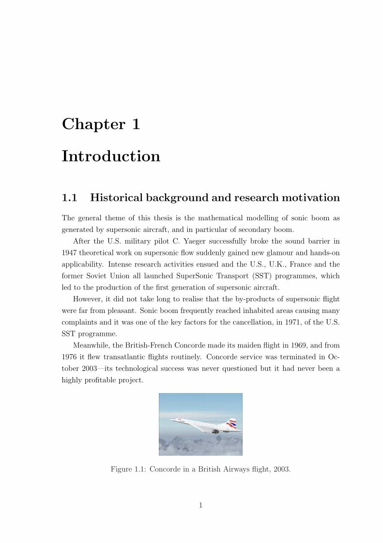
1.1 Concorde in a British Airways flight, 2003. . . . . . . . . . . . . . . . 1
1.2 The wavefront patterns due to a supersonic motion (left) and due to
a subsonic motion (right). In the supersonic case the wavefronts form
an envelope but in the subsonic case they are nested. . . . . . . . . . 4
1.3 Sonic boom carpet and pressure signatures, for an aircraft flying in a
straight line and accelerating through the sound speed to a cruise flight
with Mach 2. Primary boom is discussed in Section 1.2.1, secondary
boom in 1.2.2, focused boom and caustics in 1.2.3, and shadow-zone
boom in 1.2.4. . . . . . . . . . . . . . . . . . . . . . . . . . . . . . . . 4
1.4 A typical pressure-time history of secondary sonic boom, recorded in
Malden, New England, during Concorde’s approach to JFK airport
(British Airways Flight BA-171), on 18-07-1979—from Rickley and
Pierce [104], p.71. . . . . . . . . . . . . . . . . . . . . . . . . . . . . . 5
1.5 A schematic illustrating a direct and an indirect secondary boom. . . 6
1.6 Schematic of the far-field wave pattern from a supersonic aircraft, in a
frame moving with the aircraft—from [76]. . . . . . . . . . . . . . . . 9
2.1 Closed material curve C(t) cut by shocks at positions Pi(t). Here
1 ≤ i ≤ 4. . . . . . . . . . . . . . . . . . . . . . . . . . . . . . . . . . 22
3.1 Ray cone for a uniform medium (c0 = 1), in the (x, z, t) space. . . . . 31
3.2 Wavefronts generated by a stationary point source in a uniform medium. 31
3.3 M0 < 1: the wavefronts are nested, so no envelope is formed. . . . . . 35
3.4 M0 > 1: the wavefronts form an envelope. In two dimensions the
envelope is a Mach wedge with opening semiangle the Mach angle
θM0 = arcsin(1/M0). . . . . . . . . . . . . . . . . . . . . . . . . . . . 36
v

3.5 Visualisation of a two-dimensional supersonic motion in the (x, z, t)-
space (U =√
2, c0 = 1), for a point source moving in the negative
x-direction. The source path x = −Ut, z = 0, is displayed by a solid
straight line and its projection onto the (x, z)-plane by a solid arrow.
The two boomrays, at angle θB0 = ±π/4 to the direction of motion, are
marked on each ray cone (only the family with θB0 = −π/4 is clearly
visible here). . . . . . . . . . . . . . . . . . . . . . . . . . . . . . . . . 38
3.6 The view of Figure 3.5 in the (x, z)-space. Both families of boomrays
are shown. . . . . . . . . . . . . . . . . . . . . . . . . . . . . . . . . . 39
3.7 Selected wavefronts: for t0 < tc = 2/3 we show t0 = 1/3, t0 = 1/2. The
marginal wavefront tc = 2/3 is marked with a thicker line. The cusped
wavefronts t0 = (1 +√
2)/3, 2√
2/3,√
3/2 and 4√
2/3 are shown. As
explained in the text, for t0 < tc the wavefront has a vertical tangent
only at one point, for tc < t0 < 2√
2/3 at two points and nowhere for
t0 > 2√
2/3. The caustic (locus of cusps) z = 1− x2/4 is plotted with
a dashed line. . . . . . . . . . . . . . . . . . . . . . . . . . . . . . . . 45
3.8 The local behaviour of the wavefronts for ε = 0 (left) and ε = 0.01
(right). When ε = 0 there is a discontinuity in the curvature at x =
0, z = 1, t0 = 2/3. The exact wavefronts are plotted with dashed lines. 46
3.9 t = 2/3: ray conoid. . . . . . . . . . . . . . . . . . . . . . . . . . . . . 47
3.10 t = 2/3: rays. . . . . . . . . . . . . . . . . . . . . . . . . . . . . . . . 48
3.11 t =2√
2
3: rays in the (x, z, t)-space. . . . . . . . . . . . . . . . . . . . 48
3.12 t =2√
2
3: wavefront and rays. The cusp-rays (defined in the text),
dividing the behaviour into upper and lower branch rays are plotted
with a thicker line. . . . . . . . . . . . . . . . . . . . . . . . . . . . . 49
3.13 The Airy function of the first kind, Ai(x) and the Airy function of the
second kind Bi(x) (left and right plot respectively). . . . . . . . . . . 52
3.14 Diagram of α = α/ω versus z illustrating the four regions I, II, III and
IV as discussed in the text. . . . . . . . . . . . . . . . . . . . . . . . . 54
3.15 <(U), ω = 10. . . . . . . . . . . . . . . . . . . . . . . . . . . . . . . . 55
3.16 =(U), ω = 10. . . . . . . . . . . . . . . . . . . . . . . . . . . . . . . . 56
3.17 Contour plots for <(U) and =(U), ω = 10. . . . . . . . . . . . . . . . 56
3.18 |U |, ω = 10. . . . . . . . . . . . . . . . . . . . . . . . . . . . . . . . . 57
3.19 <(U), ω = 30. . . . . . . . . . . . . . . . . . . . . . . . . . . . . . . . 57
3.20 =(U), ω = 30. . . . . . . . . . . . . . . . . . . . . . . . . . . . . . . . 58
vi
3.21 Contour plots for <(U) and =(U), ω = 30. . . . . . . . . . . . . . . . 58
3.22 |U |, ω = 30. . . . . . . . . . . . . . . . . . . . . . . . . . . . . . . . . 59
3.23 Contour plots of t2(x, z)− t1(x, z) as n varies. . . . . . . . . . . . . . 60
3.24 Characteristics of the Tricomi-type equation (3.106). . . . . . . . . . 62
3.25 U =√
2, c0 = 1: Mach envelope as envelope of wavefronts in the
medium c = 1/√
1− z. The locus of cusps (as described in the text)
is also shown (dashed curve). The sonic line is at z = 1/2, and also
plotted with a dashed line. . . . . . . . . . . . . . . . . . . . . . . . . 63
3.26 Schematic diagrams for the formation of the incident and reflected
parts of the Mach envelope (left and right respectively). In each case
the thin curves are the wavefronts and the thick curve is their envelope. 63
3.27 U =√
2, c0 = 1: Boomrays and the Mach envelope made up as the
locus of their tips. The boomrays that form the reflected part of the
envelope have touched a fold caustic. The Mach envelope and the sonic
line are plotted with a dashed line. . . . . . . . . . . . . . . . . . . . 66
3.28 Subsonic motion with U = 1/2 in the stratified medium c = 1/√
1− z.
For t = 2, we show 12 wavefronts τ = n/6, n = 0, ..., 11. The sonic line
z = −3 and the locus of cusps (3.110) are also shown (with a dashed
line). . . . . . . . . . . . . . . . . . . . . . . . . . . . . . . . . . . . . 68
3.29 X-sections of the Mach conoid (3.140) for increasing X: for X0 < Xc =
2/3 we show X0 = 1/3 and X0 = 1/2. The marginal section X0 = 2/3
is marked with a thicker line. The cusped sections X0 = (1 +√
2)/3,
2√
2/3,√
3/2 and 4√
2/3 are shown. Apart from the axes, this figure
is exactly the same as Figure 3.7. . . . . . . . . . . . . . . . . . . . . 71
3.30 BICHs for the model atmosphere with local Prandtl-Glauert parameter
B2 = 1−z. They are stopped at z = zg = −1/2 and the corresponding
carpet is plotted. The ϕ = π/2 BICH (plotted with a thicker red line)
has its maximum at the sonic line z = 1. This maximum is a Tricomi
cusp. . . . . . . . . . . . . . . . . . . . . . . . . . . . . . . . . . . . . 73
3.31 The carpet for B2 = 1 − z at z = zg = −1/2. The primary and sec-
ondary carpets are joined because all BICHs launched upwards, even-
tually reach zg. . . . . . . . . . . . . . . . . . . . . . . . . . . . . . . 74
3.32 B2 = 1− z: BICHs reflecting off the z-level zg = −1/2. . . . . . . . 75
vii

3.33 B2 = 1 − z: the carpet when we take into account reflection at
zg = −1/2. From left to right, the first closed curve is the carpet of
Figure 3.31. The second closed curve is a “reflected” carpet; it consists
of a part (solid line) formed by the reflected PC BICHs and a part
(dashed line) that is formed by the reflected SC BICHs. . . . . . . . . 76
3.34 Typical sound speed profile for a real atmosphere (left) and the B2
profile (right). . . . . . . . . . . . . . . . . . . . . . . . . . . . . . . . 76
3.35 Mach surface for a typical stationary atmosphere, calculated numerically. 77
3.36 The carpet: PC, SC and indirect SC . . . . . . . . . . . . . . . . . . 77
3.37 B2 = 1 − |z|: BICHs that hit zg = −1/2 are shown (z0 = 0). Some
BICHs never hit zg. The limiting (grazing) BICHs are shown with a
blue colour. The PC and SC are shown with solid curves, plotted using
the analytical expressions (3.155) and (3.156). . . . . . . . . . . . . . 79
3.38 B2 = 1−|z|: the first open curve from the left is the PC at zg = −1/2,
and the second open curve is the SC. . . . . . . . . . . . . . . . . . . 80
3.39 The y = 0 section of the Mach surface: Tricomi cusps are visible. The
horizontal line at 50 km facilitates understanding of Figure 3.40 below. 81
3.40 An (x, y)-cut of the Mach surface at z = 50 km. The solid line curves
track the behaviour of BICHs that were launched upwards (0 ≤ ϕ ≤ π)
and the dashed line curves track the behaviour of BICHs that were
launched downwards (π ≤ ϕ ≤ 2π). . . . . . . . . . . . . . . . . . . . 82
3.41 Ray pattern and wavefronts for a stationary source in the stratified
medium c = 2− exp(−z2), before focusing has begun. . . . . . . . . . 85
3.42 c = 2 − exp(−z2), rays and their focusing leading to the formation of
a caustic (t = 4). . . . . . . . . . . . . . . . . . . . . . . . . . . . . . 85
3.43 c = 2 − exp(−z2), the folded wavefronts are shown (t = 4) taken at
time intervals ∆t = 0.1. . . . . . . . . . . . . . . . . . . . . . . . . . . 86
3.44 Photograph and sketch of rays for the coffee-cup caustic. . . . . . . . 87
4.1 A body for which the induced supersonic flow can be analysed with
two-dimensional theory. . . . . . . . . . . . . . . . . . . . . . . . . . 99
4.2 An aerofoil with thickness function G(x) and chord L, symmetric with
respect to the x-axis. . . . . . . . . . . . . . . . . . . . . . . . . . . . 99
4.3 Flow pattern above a supersonic thin aerofoil, showing the contrast
between linear and nonlinear theory. Only the z > 0 plane is shown
(assuming an aerofoil symmetric with respect to the x-axis). . . . . . 103
viii
4.4 The upper part of an aerofoil with thickness function G(x) (thicker
line) and G′(x) which has a positive and negative part in relation to
the undisturbed value G′ = 0 (since G(−1/2) = G(1/2) the areas under
the positive and negative part are equal). . . . . . . . . . . . . . . . . 108
4.5 The characteristic diagram with the shock paths for the parabolic
thickness function. . . . . . . . . . . . . . . . . . . . . . . . . . . . . 110
4.6 The profile of u. . . . . . . . . . . . . . . . . . . . . . . . . . . . . . . 111
4.7 Schematic that shows the relation between the characteristic labels ξ1
and ξ2 mentioned in the text. . . . . . . . . . . . . . . . . . . . . . . 112
4.8 The asymptoticN -wave profile. A is the area under the positive/negative
part and D =(γ + 1)M4
0
2B0
. . . . . . . . . . . . . . . . . . . . . . . . . 114
4.9 A (slender) axisymmetric body and the chosen system of cylindrical
polar coordinates. . . . . . . . . . . . . . . . . . . . . . . . . . . . . . 114
4.10 A meridional section of a slender body of revolution (which is nondi-
mensionalised on the chord length). . . . . . . . . . . . . . . . . . . . 115
4.11 The difference between planar and axisymmetric problems is sketched.
In axisymmetric flow the wave has a “tail” as explained in the text. . 120
6.1 Schematic of the Mach wedge and the initial wavefront (IW). The
point A1 is outside the IW and A2 is inside the IW. (The horizontal
line represents the path of the source.) . . . . . . . . . . . . . . . . . 145
6.2 The quadratic Q at two points inside the Mach wedge, A1 outside the
IW (left plot) and A = A2 (right plot). The points A1 and A2 are
shown in Figure 6.1. On the left plot both roots of Q are positive but
on the right plot τ1 has become negative. (We have chosen c0 = 1,
U =√
2, t = 3.) . . . . . . . . . . . . . . . . . . . . . . . . . . . . . . 146
6.3 Plot of 2πp0s where p0s is the wavefield inside the IW when the point
source travels with constant speed from right to left, U =√
2,c0 = 1,t =
3. . . . . . . . . . . . . . . . . . . . . . . . . . . . . . . . . . . . . . . 147
6.4 The Mach envelope for the times t = 1.2, 1.5, 2, 3, generated by a point
source moving with constant acceleration from right to left. The cusp
locus (thicker, red line) is plotted along with the wavefront x2 +z2 = t2?
(dotted blue line), where t? = 2 is the time at which the source catches
up with its initial disturbance. . . . . . . . . . . . . . . . . . . . . . . 151
ix
6.5 The boomrays form a fold caustic (t = 3), shown with a thicker red
line. The boomrays passing through the cusps (τE = t1/3) are plotted
with green. The Mach envelope is plotted with a dashed line. . . . . . 152
6.6 Two boomrays at distance ε apart, emitted from points A and B at
time difference ∆τ , meeting at a point F . . . . . . . . . . . . . . . . . 153
6.7 The wavefront pattern generated by an accelerating source from right
to left (t = 3). . . . . . . . . . . . . . . . . . . . . . . . . . . . . . . . 155
6.8 Schematic diagrams for the formation of the front and back parts of
the Mach envelope (left and right respectively). In each case the thin
curves are the wavefronts and the thick curve is their envelope. . . . . 155
6.9 The formation of the back envelope (t = 3): The Mach envelope and
the fold caustics are plotted with green and red respectively. We plot
the wavefront τ = t1/3 passing through the cusps C1 and C2 and the
associated boomrays; we also plot the wavefront τ = 1 touching the
back envelope at the point D where the boomrays coalesce. The wave-
fronts for the values of τ between 1 and t1/3 always cross the front
envelope and therefore have two distinct contact points that touch the
back envelope from outside. . . . . . . . . . . . . . . . . . . . . . . . 157
6.10 Plot of the Mach envelope, the initial wavefront and indication of the
typical points A, B, C, D, E, F and G. . . . . . . . . . . . . . . . . . 160
6.11 Plot of Q at points A, B, C, D, E, F and G in Figure 6.10. . . . . . 160
6.12 Pressure jump on the front envelope. . . . . . . . . . . . . . . . . . . 163
6.13 Plot of f(τE, t) as a function of τE, where −2f(τE, t) is the strength of
the logarithmic singularity. . . . . . . . . . . . . . . . . . . . . . . . 167
6.14 t = M0: wavefront pattern and boomrays. . . . . . . . . . . . . . . . 170
6.15 The Mach envelope for t = M0 − 1.25,M0 − 1,M0,M0 + 1 (M0 = 1.5).
The dotted part is the steady supersonic motion envelope and the solid
line part is the deceleration envelope. . . . . . . . . . . . . . . . . . . 171
6.16 For a convex function the slope of the chord AB is less than the slope
of the chord BC. . . . . . . . . . . . . . . . . . . . . . . . . . . . . . 172
6.17 The envelope and the initial wavefront for t = M0 − 1. In Figure 6.18
we plot the behaviour of Q at the points A, B, O, C and D. . . . . . 174
6.18 Plot of Q at points A, B, O, C and D as shown in Figure 6.17. . . . 174
6.19 The pressure jump on the deceleration envelope, for−(M0 − 1) ≤ τE ≤M0 − 1,
t = M0 (M0 = 1.5). . . . . . . . . . . . . . . . . . . . . . . . . . . . . 176
x
6.20 The wavefront pattern for a circular motion with radius R0 = 0.75 < 1
and angular velocity θ = 1. . . . . . . . . . . . . . . . . . . . . . . . . 179
6.21 Circular motion with constant angular velocity (M0 = 2 with R0 = 2
and θ = 1). . . . . . . . . . . . . . . . . . . . . . . . . . . . . . . . . 179
6.22 Motion in a circle with non-constant angular velocity (R0 = 2, θ = τ). 180
6.23 Motion in a parabolic trajectory x0(τ) = τ, z0(τ) = τ 2: we take t = 1
and −1 ≤ τ ≤ t = 1. . . . . . . . . . . . . . . . . . . . . . . . . . . . 181
6.24 Constant acceleration in the stratified medium with sound speed profile
c = 1/√
1− z: Boomrays for t = 3, τ = 1.1 to τ = 2.9, in increments
of 0.05. . . . . . . . . . . . . . . . . . . . . . . . . . . . . . . . . . . . 183
6.25 Constant acceleration in the stratified medium with sound speed profile
c = 1/√
1− z. The boomrays are ilustrated for t = 3, τ = 1.01
to τ = 2.9 (in increments of 0.01). The Mach envelope formed by
the boomrays launched upwards is drawn with green and the Mach
envelope formed by the boomrays launched downwards is drawn with
red. . . . . . . . . . . . . . . . . . . . . . . . . . . . . . . . . . . . . . 183
6.26 Wavefronts for t = 3: only supersonic part of the motion. . . . . . . . 184
6.27 The Mach envelope for t = 3, t = 5, t = 8. (The envelope for t = 8 is
very elongated in the x-direction and not all of it shown.) . . . . . . . 185
6.28 The Mach envelope for t = 20 and t = 21: magnified view near the new
cusps which correspond to the formation of a cusp caustic of boomrays.
The lower Tricomi cusps are also shown on each of the two envelope. 185
6.29 A perfect focus of boomrays (motion in a straight line). . . . . . . . . 186
6.30 A perfect focus of boomrays: motion in an equiangular spiral. . . . . 187
6.31 The trace of the fold caustic at the ground. The (x, y)-cut of the fold
caustic at the height of the source (z = 0) is also plotted (with a dashed
line). . . . . . . . . . . . . . . . . . . . . . . . . . . . . . . . . . . . . 190
7.1 Characteristics for the linear problem. The various regions marked
correspond to values of u as explained in the text. . . . . . . . . . . . 194
7.2 Focusing of the Type2R characteristics (A = 1) . . . . . . . . . . . . 198
7.3 A = 0.05: the shocks and some important characteristics are plotted
here. The value of u as parametrised by τ (or τ ′ as appropriate) is also
noted in the various regions. The merging of the shocks occurs above
the source path. . . . . . . . . . . . . . . . . . . . . . . . . . . . . . . 203
xi
7.4 A = 0.2: the shocks are shown. Now the merging happens before the
source path. The sonic tangent and the τ = 1 characteristics are shown
with dotted lines. The various regions of u values are indicated. . . . 206
7.5 A = 1/2: the shocks, the characteristics entering the common point of
ShockI and ShockIII, the sonic tangent and the τ = 1 characteristic
are shown. The various regions of u values are indicated. . . . . . . . 207
7.6 A=0.05: snapshot of the wavefield at the sonic time t = 1: u(x, 1) and
the perturbation v(x, 1) =u(x, 1)− 1
A. . . . . . . . . . . . . . . . . . 208
7.7 A = −0.2: the shock and the expansion fan (region inside the dashed
lines on the right of the shock). The characteristics entering the point
joining the first and second part of the shock are also shown. The
various regions of u are indicated. . . . . . . . . . . . . . . . . . . . . 210
7.8 A = −1: details of the behaviour near the origin. The shock has a
turning point corresponding to τTP = 2/3(−2 +√
7) = 0.43. We plot
the characteristics entering this turning point from the left and from
the right. . . . . . . . . . . . . . . . . . . . . . . . . . . . . . . . . . . 211
7.9 A = −0.2: snapshot of the wavefield at the sonic time t = 1. The
snapshot u(x, 1) is plotted with a solid line and the snapshot v(x, 1) =
(u− 1)/A is plotted with a dotted line. . . . . . . . . . . . . . . . . . 212
C.1 A = 0.05: characteristic diagram that shows the six different types
of behaviour a snapshot of the wavefield may have. The regions are
separated with horizontal dotted lines and each region is marked with
WF1, WF2, WF3 and so on. . . . . . . . . . . . . . . . . . . . . . . . 231
C.2 Snapshots for A = 0.05 for times t = 0.75, 1 + 0.5√
2A = 1.158, 1.5. . 232
C.3 A = 1: characteristic diagram showing the four cases of different wave-
field behaviour. . . . . . . . . . . . . . . . . . . . . . . . . . . . . . . 233
C.4 A = 1: snapshots at times t0 = 0.5, 1.5, 2.924, 4. Each snapshot be-
longs to a different time regime as explained in the text. . . . . . . . 234
C.5 A = −0.2: characteristic diagram with horizontal lines marking the
times t = 1 −√
2|A| = 0.367, t =√
1− 2|A| = 0.774, t = 2, tshock =
4.211 dividing the five cases of different wavefield behaviour. . . . . . 235
C.6 A = −0.2: wavefield snapshots for t = (1−√
2|A|)/2 = 0.184, 1.25, 1.8, 3.
These correspond respectively to the first four cases. . . . . . . . . . . 235
xii
Chapter 1
Introduction
1.1 Historical background and research motivation
The general theme of this thesis is the mathematical modelling of sonic boom as
generated by supersonic aircraft, and in particular of secondary boom.
After the U.S. military pilot C. Yaeger successfully broke the sound barrier in
1947 theoretical work on supersonic flow suddenly gained new glamour and hands-on
applicability. Intense research activities ensued and the U.S., U.K., France and the
former Soviet Union all launched SuperSonic Transport (SST) programmes, which
led to the production of the first generation of supersonic aircraft.
However, it did not take long to realise that the by-products of supersonic flight
were far from pleasant. Sonic boom frequently reached inhabited areas causing many
complaints and it was one of the key factors for the cancellation, in 1971, of the U.S.
SST programme.
Meanwhile, the British-French Concorde made its maiden flight in 1969, and from
1976 it flew transatlantic flights routinely. Concorde service was terminated in Oc-
tober 2003—its technological success was never questioned but it had never been a
highly profitable project.
Figure 1.1: Concorde in a British Airways flight, 2003.
1
However, it is highly probable that civil supersonic aviation will be reinstated in
the future, as the travel market is steadily growing, both for leisure and business
purposes. Hence sonic boom research is currently undergoing a renaissance.
The human response to aircraft noise [116] is complicated because of the multi-
tude of factors involved such as previous exposure, geographic location, time of day,
socioeconomic status etc1. Sonic boom contributes an additional environmental noise
impact, specific to supersonic flight. As of 1973, civil supersonic flights are forbidden
above land [3]. However, the long-term effects on health of daily exposure to sonic
booms are yet to be investigated, and a quantitative measure of acceptability has not
been established. It is however commonly accepted that loud and unexpected noises
tend to disorient and startle people, and studies indicate that reaction to sonic boom
is far more severe than reaction to other types of noise at analogous amplitude levels
[79, 114]. Furthermore, there are fears that sonic boom will pose a threat to aquatic
life, and to fowl, farm and wild animals [36]. Therefore, the environmental impact
of sonic boom needs to be carefully evaluated and precise noise regulations for sonic
boom need to be devised. Such regulations could substantially limit the profitability
of a new SST or stop its implementation altogether.
For successful mitigation of the annoyance due to sonic boom, a thorough under-
standing of the generation and propagation of the relevant acoustic waves is required.
Such an understanding should lead to new predictions and modifications in aircraft
design and operation that would limit the impact of sonic boom. In Section 1.2 we
explain what a sonic boom is and classify the different forms in which it is heard at
the ground, in Section 1.3 we discuss the current state of sonic boom research, and
in Section 1.4 we give an outline of this thesis.
1.2 Sonic boom
A shock-wave pattern is formed around an aircraft when flying at supersonic speed
(i.e. faster than sound). Sonic boom is the noise from these shock waves, as heard at
the ground. Sonic booms are weak shocks: the typical overpressure at the ground is
up to 100 Pa, a shock strength of order 10−3 of the atmospheric pressure [126].
For weak shocks nonlinearities can be neglected, to a first approximation, and the
disturbance due to the motion of a supersonic aircraft can be thought of as the linear
1Sound is recorded in Pa or dB. However there are various metrics that estimate the soundperceived by a human ear. Such noise metrics, as formally stated by the U.S. Federal Aviation Ad-ministration (see http://www.nonoise.org/library/ane/ane.htm), are the A-Weighted Sound Level(AL), Sound Exposure Level (SEL), Yearly Average Day Night Level (DNL) metric etc.
2
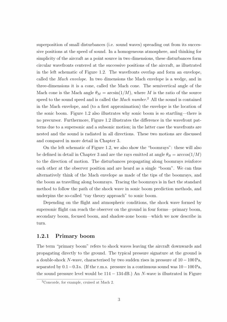
superposition of small disturbances (i.e. sound waves) spreading out from its succes-
sive positions at the speed of sound. In a homogeneous atmosphere, and thinking for
simplicity of the aircraft as a point source in two dimensions, these disturbances form
circular wavefronts centered at the successive positions of the aircraft, as illustrated
in the left schematic of Figure 1.2. The wavefronts overlap and form an envelope,
called the Mach envelope. In two dimensions the Mach envelope is a wedge, and in
three-dimensions it is a cone, called the Mach cone. The semivertical angle of the
Mach cone is the Mach angle θM = arcsin(1/M), where M is the ratio of the source
speed to the sound speed and is called the Mach number.2 All the sound is contained
in the Mach envelope, and (to a first approximation) the envelope is the location of
the sonic boom. Figure 1.2 also illustrates why sonic boom is so startling—there is
no precursor. Furthermore, Figure 1.2 illustrates the difference in the wavefront pat-
terns due to a supersonic and a subsonic motion; in the latter case the wavefronts are
nested and the sound is radiated in all directions. These two motions are discussed
and compared in more detail in Chapter 3.
On the left schematic of Figure 1.2, we also show the “boomrays”: these will also
be defined in detail in Chapter 3 and are the rays emitted at angle θB = arccos(1/M)
to the direction of motion. The disturbances propagating along boomrays reinforce
each other at the observer position and are heard as a single “boom”. We can thus
alternatively think of the Mach envelope as made of the tips of the boomrays, and
the boom as travelling along boomrays. Tracing the boomrays is in fact the standard
method to follow the path of the shock wave in sonic boom prediction methods, and
underpins the so-called “ray theory approach” to sonic boom.
Depending on the flight and atmospheric conditions, the shock wave formed by
supersonic flight can reach the observer on the ground in four forms—primary boom,
secondary boom, focused boom, and shadow-zone boom—which we now describe in
turn.
1.2.1 Primary boom
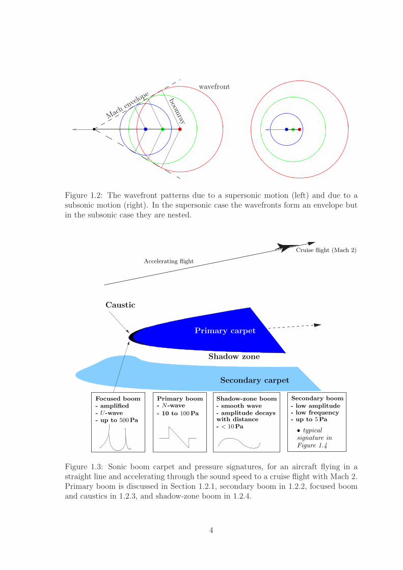
The term “primary boom” refers to shock waves leaving the aircraft downwards and
propagating directly to the ground. The typical pressure signature at the ground is
a double-shock N -wave, characterised by two sudden rises in pressure of 10− 100 Pa,
separated by 0.1−0.3 s. (If the r.m.s. pressure in a continuous sound was 10−100 Pa,
the sound pressure level would be 114− 134 dB.) An N -wave is illustrated in Figure
2Concorde, for example, cruised at Mach 2.
3
boomray
wavefront
Machenv
elope
Figure 1.2: The wavefront patterns due to a supersonic motion (left) and due to asubsonic motion (right). In the supersonic case the wavefronts form an envelope butin the subsonic case they are nested.
���������������������
���������������������
���������
���������
Focused boom Shadow-zone boom
Secondary carpet
Caustic
Shadow zone
Primary boom
Figure 1.4
- amplified- U-wave- up to 500Pa
- N-wave
- 10 to 100Pa- smooth wave- amplitude decays
signature in• typical
Cruise flight (Mach 2)
- < 10Pawith distance
Primary carpet
Accelerating flight
Secondary boom- low amplitude- low frequency- up to 5Pa
Figure 1.3: Sonic boom carpet and pressure signatures, for an aircraft flying in astraight line and accelerating through the sound speed to a cruise flight with Mach 2.Primary boom is discussed in Section 1.2.1, secondary boom in 1.2.2, focused boomand caustics in 1.2.3, and shadow-zone boom in 1.2.4.
4
1.3 (second plot from the left). The primary carpet, defined as the area on the ground
where primary boom is heard, is a strip of land directly below the aircraft, as also
illustrated in Figure 1.3. Primary boom is the most annoying type of boom, and has
also been known to cause structural damage [76].
1.2.2 Secondary boom
Secondary Sonic Boom (SSB) or over-the-top boom, is due to shock waves that are
returned to the ground by temperature or wind gradients in the atmosphere above
the aircraft. The presence of SSB was not given due consideration until routine
operation of Concorde was established. SSB is less annoying than primary boom but
may cause easily observable building vibration and rattling [76]. The evaluation of
its community acceptance is still at a very early stage.
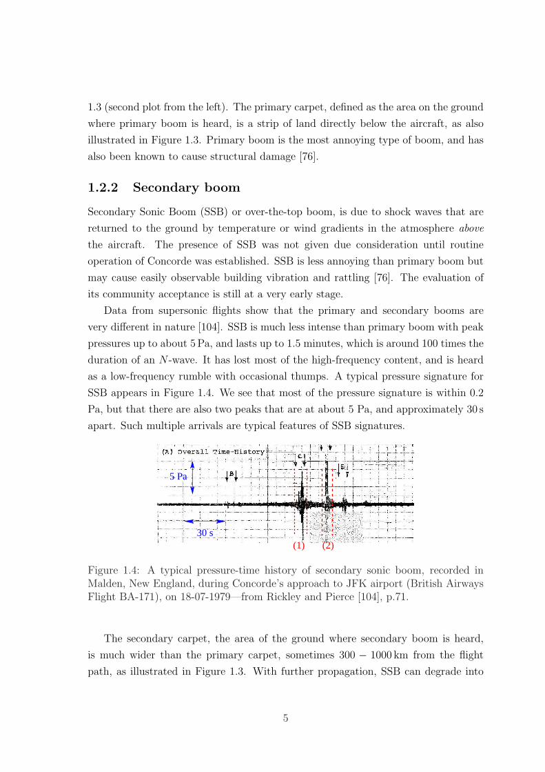
Data from supersonic flights show that the primary and secondary booms are
very different in nature [104]. SSB is much less intense than primary boom with peak
pressures up to about 5 Pa, and lasts up to 1.5 minutes, which is around 100 times the
duration of an N -wave. It has lost most of the high-frequency content, and is heard
as a low-frequency rumble with occasional thumps. A typical pressure signature for
SSB appears in Figure 1.4. We see that most of the pressure signature is within 0.2
Pa, but that there are also two peaks that are at about 5 Pa, and approximately 30 s
apart. Such multiple arrivals are typical features of SSB signatures.
5 Pa
30 s(1) (2)
Figure 1.4: A typical pressure-time history of secondary sonic boom, recorded inMalden, New England, during Concorde’s approach to JFK airport (British AirwaysFlight BA-171), on 18-07-1979—from Rickley and Pierce [104], p.71.
The secondary carpet, the area of the ground where secondary boom is heard,
is much wider than the primary carpet, sometimes 300 − 1000 km from the flight
path, as illustrated in Figure 1.3. With further propagation, SSB can degrade into
5
an infrasonic disturbance that can travel thousands of miles under certain weather
conditions.
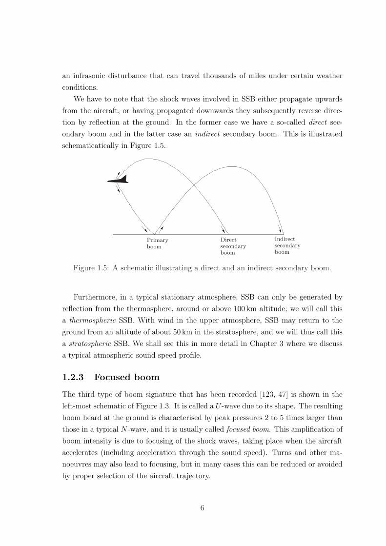
We have to note that the shock waves involved in SSB either propagate upwards
from the aircraft, or having propagated downwards they subsequently reverse direc-
tion by reflection at the ground. In the former case we have a so-called direct sec-
ondary boom and in the latter case an indirect secondary boom. This is illustrated
schematicatically in Figure 1.5.
boomPrimary Direct
secondaryboom
Indirectsecondaryboom
Figure 1.5: A schematic illustrating a direct and an indirect secondary boom.
Furthermore, in a typical stationary atmosphere, SSB can only be generated by
reflection from the thermosphere, around or above 100 km altitude; we will call this
a thermospheric SSB. With wind in the upper atmosphere, SSB may return to the
ground from an altitude of about 50 km in the stratosphere, and we will thus call this
a stratospheric SSB. We shall see this in more detail in Chapter 3 where we discuss
a typical atmospheric sound speed profile.
1.2.3 Focused boom
The third type of boom signature that has been recorded [123, 47] is shown in the
left-most schematic of Figure 1.3. It is called a U -wave due to its shape. The resulting
boom heard at the ground is characterised by peak pressures 2 to 5 times larger than
those in a typical N -wave, and it is usually called focused boom. This amplification of
boom intensity is due to focusing of the shock waves, taking place when the aircraft
accelerates (including acceleration through the sound speed). Turns and other ma-
noeuvres may also lead to focusing, but in many cases this can be reduced or avoided
by proper selection of the aircraft trajectory.
6
Similar focusing also occurs in the atmosphere due to the inhomogeneous sound
speed. In a stationary stratified atmosphere focusing occurs at some height, in or be-
low the thermosphere, where the boom is reflected downwards.3 The issue of focusing
is therefore relevant to the propagation route by which secondary boom reaches the
observer on the ground.
The three focusing scenarios discussed above are geometrically similar, and involve
the production of a U -wave. Because of this, and because secondary boom can itself
be focused4, in this thesis we will also give attention to accelerating motions and
manoeuvres.
1.2.4 Shadow-zone boom
The gap between the primary and secondary carpets shown in Figure 1.3 occurs
because part of the shock wave is trapped in an atmospheric waveguide and never
reaches the ground. This will be explained in more detail in Chapter 3.
At the boundary of the primary carpet with the gap region the pressure signature
is attenuated and loses its N -wave characteristic due to ground impedance effects and
diffraction. A schematic of this fourth type of boom signature is included in Figure
1.3. This boom is usually called the “shadow-zone boom”, because it is analogous to
the propagation of light by creeping rays over the unlit surface of a curved obstacle
[18].
1.3 Current state of sonic boom research
The basic theory of sonic boom has been delineated in [124, 125, 45, 54] and im-
plemented into practical models in [54, 120, 13, 24, 98, 106]. The basic sonic boom
theory mainly concerns primary booms from steady level flight. Much of this work
was accomplished by the early 1970’s, and was largely motivated by the SST effort.
However, secondary boom, focused boom and shadow-zone boom are subjects of
continuing investigation. Below we will present the major results for the four types
of boom, and outline some of the open questions.
3The boomray launched upwards in the plane of flight reflects at the height where the soundspeed is equal to the aircraft speed, usually called the sonic height ; those launched obliquely reflectlower. More details are given in Chapter 3, and illustrated with examples.
4Figure 1.3 illustrates only focusing of primary boom, but acceleration may also cause focusingof secondary boom.
7
1.3.1 Primary boom
The first theoretical results on sonic boom came from the ballistic projectiles commu-
nity: within sonic boom nomenclature the flow pattern from a projectile is precisely
the shock-wave pattern due to a supersonic flight. In 1946 Landau analysed the
weak shock waves from a supersonic projectile and predicted an N -wave shape for
the pressure signature in the far-field [67] (i.e. at distances large compared with the
body dimensions). Soon afterwards, measurements of projectiles confirmed Landau’s
predictions [35].
In 1952, Whitham wrote a seminal paper for sonic boom research [124]. In this
he explained in detail the generation of the flow pattern from a ballistic projectile
and made it clear that sonic boom is a steady state phenomenon; it is generated
continuously as the aircraft flies supersonically and not only at the moment that the
aircraft breaks the sound barrier.
Near the aircraft (near-field), the pressure field is directly dependent on the ge-
ometry and the aerodynamics of the vehicle. Supersonic aircraft aerodynamics is
most easily computed by linearised supersonic flow theory [50, 39, 70, 126] and it is
presented in the normalised form of the so-called Whitham function [124, 126]. More
recently, with the advent of increased computing power, CFD methods have been
devised to calculate the near-field signature [89, 20, 100], but they are still under de-
velopment and not in wide use. However, shocks, even when very weak, are inherently
nonlinear. According to the linearised supersonic flow theory shock waves travel at
the sound speed, but in reality the speed of a shock wave is greater than the sound
speed and amplitude-dependent, and it turns out that at large distances from the
aircraft the weak nonlinearities have an important cumulative effect [124]. Whitham
has shown that nonlinear effects can be easily incorporated by shifting appropriately
the characteristics predicted by the linear theory, while still using the amplitudes
predicted by the linear solution [124, 125]. This is the famous Whitham’s rule. It
has been used extensively in sonic boom research (and it is discussed in great detail
in Chapter 4).
For a pointed aerofoil or axisymmetric body there are generally two shock waves,
one attached to the front (usually called the bow shock) and the other attached to
the tail (usually called the tail shock)—see, for instance, [126, 70].
An aircraft is a non-smooth body and in the near-field the shock-wave pattern
contains several shock waves, corresponding to the various compressions caused by
the detailed shape of the aircraft. However, away from the aircraft the shock wave
pattern distorts and steepens, and in the far-field it coalesces into only a bow and a tail
8
shock, as in the case of a simpler, smooth body. Records from flight tests substantiate
this since the N -wave signatures for various aircraft of similar size and weight are
essentially the same [76]. In this thesis we will study the paradigm problems of a
pointed aerofoil and a slender body—work on more complicated body shapes appears
in [50, 52, 74, 122, 125, 38].
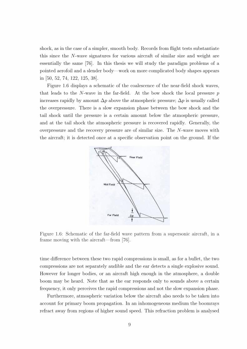
Figure 1.6 displays a schematic of the coalescence of the near-field shock waves,
that leads to the N -wave in the far-field. At the bow shock the local pressure p
increases rapidly by amount ∆p above the atmospheric pressure; ∆p is usually called
the overpressure. There is a slow expansion phase between the bow shock and the
tail shock until the pressure is a certain amount below the atmospheric pressure,
and at the tail shock the atmospheric pressure is recovered rapidly. Generally, the
overpressure and the recovery pressure are of similar size. The N -wave moves with
the aircraft; it is detected once at a specific observation point on the ground. If the
Figure 1.6: Schematic of the far-field wave pattern from a supersonic aircraft, in aframe moving with the aircraft—from [76].
time difference between these two rapid compressions is small, as for a bullet, the two
compressions are not separately audible and the ear detects a single explosive sound.
However for longer bodies, or an aircraft high enough in the atmosphere, a double
boom may be heard. Note that as the ear responds only to sounds above a certain
frequency, it only perceives the rapid compressions and not the slow expansion phase.
Furthermore, atmospheric variation below the aircraft also needs to be taken into
account for primary boom propagation. In an inhomogeneous medium the boomrays
refract away from regions of higher sound speed. This refraction problem is analysed
9
using Geometrical Acoustics (GA) in non-uniform media [17, 65]. GA is generally
a good approximation since the wavelength is much smaller than the length-scale of
propagation involved, and also the length-scale of atmospheric variation. Blokhintsev
in [17] established the GA theory for monochromatic waves in a non-uniform, moving
medium, and Keller showed in [65] that this theory also applies to weak shock waves.
Based on these theoretical results the following procedure has been widely used
in the prediction of primary sonic boom: the Whitham function is obtained for the
particular aircraft geometry, usually using linearised supersonic flow theory. Then
at a certain distance from the aircraft (which depends on its size, shape and speed),
the boomrays are launched using pressure values from the Whitham function. The
boomrays are then traced, with Whitham’s rule being applied to account for the
nonlinearities.
The codes [54, 120, 13, 106, 24, 98] generally implement the prediction method
outlined in the previous paragraph, and have been used to predict primary boom
carpets and signatures successfully. We note that each of these codes has its own
capabilities and limitations depending on the task in hand at the time; the review
[99] by Plotkin contains a brief overview of the sonic boom codes that were available
in 2002, together with a discussion of their relative merits and disadvantages.
Some open questions in primary boom research concern propagation through tur-
bulence in the lower atmosphere [30, 93, 13, 96, 95], absorption and dispersion due
to viscosity and non-equilibrium (relaxation) effects [101, 83, 115, 12, 60, 49, 62],
underwater penetration [117], and so on—these however are not within the scope of
this thesis and we will not discuss them further.
1.3.2 Secondary boom
A complete theoretical understanding of secondary boom is yet to be acquired. SSB
involves propagation over long distances and it is thus quite likely that many effects
that can be safely neglected in primary boom studies need to be taken into account.
Rogers and Gardner in [108] concluded that attenuation in the atmosphere leads
to a thermospheric SSB of insignificant amplitude. On the other hand, in [33], Donn
presented measurements of SSB traces and he interpreted them as stratospheric and
thermospheric SSBs being of similar amplitude but with the latter having lower-
frequency content. Furthermore, boomray tracing was used in [104], based on real
meteorological data and Concorde flight conditions, to predict signal arrivals within
10
20 s of those recorded (no amplitude calculations were undertaken however).5 Ad-
ditionally, the report [48] is a helpful summary of the state of knowledge of SSB in
1995, and some information is also found in the sonic boom review papers [76] and
[99].
Below we list the major open questions, prior to the SOBER programme, and
outline which of them are addressed in this thesis:
• Focusing is an important aspect of an accurate prediction of SSB, as outlined in
Section 1.2.3 above. Preliminary work on this appears in [55, 91, 41]. Further
results appear in this thesis, especially in Chapter 3, and are outlined in Section
1.4.
• We have also discussed how nonlinear effects are important in determining the
far-field signature for a primary boom. The inclusion of nonlinearities in SSB
propagation is also an interesting open problem. In Chapter 5 we develop
a paradigm model where such nonlinearities are incorporated in a consistent
manner. Other related work is in [55, 91, 108, 111, 7].
• The influence of the Coriolis effect on sound propagation in the atmosphere has
been studied by [110] and further reviewed by the author within the SOBER
programme [63]. It was found that for a propagation range of even 1000 km,
the Coriolis effect is insignificant. This was to be expected as the timescale of
SSB propagation is much smaller than a day.
• The effect of the earth’s curvature is insignificant for short-range propagation
over the earth’s surface but can become important in the kind of long-range
propagation involved in SSB. It has also been studied within the SOBER pro-
gramme by the author [63]. It was concluded that over long ranges these effects
are important, but that they can be nevertheless easily incorporated in a “flat-
earth” boomray tracing code to first order, by appropriately modifying the
sound speed profile with a linear correction.
• The low amplitudes involved in SSB and the long-wavetrain nature of the sig-
nature indicate that dissipation and dispersion due to viscosity and relaxation
effects are likely to be important. These effects on SSB have not been studied
in this thesis, but have been studied within the SOBER programme [7].
5It was subsequently concluded by the U.S Department of Transportation that SSB affectedinhabited areas in New England, and Concorde was requested to decelerate to subsonic speedsfurther away from the coast.
11
• Three-dimensional wind or temperature inhomogeneities, such as atmospheric
gravity waves, may also be a reason for the multiple arrivals observed in the
SSB signature. These effects have been studied within the SOBER programme.
Also, small-scale inhomogeneities created near the ground by turbulence may be
important for explaining the nature of the SSB signatures. To our knowledge,
these effects have not been studied as yet.
In SSB propagation many widely separated length-scales are involved and one should
be very careful before developing a numerical procedure for SSB prediction. While
the propagation distance is 300 to 1000 km, the scale of atmospheric variations is
about 10 times smaller and the aircraft length 1000 times smaller still. Consequently,
any numerical procedure would have to be able to deal with these multiple scales.
Furthermore, focusing in the upper layers of the atmosphere corresponds to a transi-
tion from a hyperbolic model to an elliptic one, and this also needs careful numerical
treatment.
Only three codes exist for prediction of SSB. The TRAPS code [119] is a re-
formulation of the primary boom code [54] that can also cater for upward-launched
boomrays. It is successful in predicting where SSB reaches the ground but it gives too
large amplitudes. To resolve this discrepancy, the ZEPHYRUS code [106] was subse-
quently written; its most important feature is the incorporation of air absorption ef-
fects and it indeed predicts lower values for the overpressures. However, ZEPHYRUS
is much more computer intensive than TRAPS. More recently, as part of the SOBER
programme a third code was constructed [31, 7]; this code includes nonlinearity, ab-
sorption and relaxation effects by various chemical species and uses real meteorolog-
ical data—it supersedes both TRAPS and ZEPHYRUS as it predicts, in reasonable
computing time, results that agree well with SSB observations. The thumps are inter-
preted as due to multipath arrivals due to direct and indirect SSB, and the rumbling
noise as an effect of atmospheric gravity waves. The conclusion in [108] that ampli-
tudes of stratospheric SSBs are larger than amplitudes of thermospheric SSBs seems
to now be supported by the results in [31, 7].
1.3.3 Focused boom
Focused boom is a topic of great interest in sonic boom research and there is a large
literature on it [59, 9, 10, 25, 11, 27]. Some details will be given here, and a more
elaborate discussion is given in Chapters 3, 6 and 7.
12
The focusing in almost any flight condition leads to a smooth envelope of boom-
rays, a fold caustic in the terminology of catastrophe theory [15]. Higher-order focus-
ing, such as that indicated by a cusped envelope of boomrays, a cusp caustic in terms
of catastrophe theory (and geometrically similar to the famous coffee-cup caustic) is
much rarer. Furthermore, perfect lens-like focusing is unlikely to occur [76].
GA predicts an infinite amplitude at caustics. For linear monochromatic waves
the amplitude near a fold caustic is determined using the well-established Geometrical
Theory of Diffraction [66, 19, 75], which re-introduces diffraction to first order in an
appropriately defined Diffraction Boundary Layer (DBL) in the neighbourhood of the
caustic. This leads to a linear Tricomi equation.
In the focusing of weak shock waves, for an N -wave incident on a fold caustic
the linear Tricomi equation gives rise to a reflected wave which is a U -wave with
infinite peaks [109]. Such singularities are an unphysical result. The established
modelling approach for eliminating these singularities is to combine diffraction effects
with nonlinear effects. This procedure leads to a so-called nonlinear Tricomi equation,
first derived by Guiraud in [45] and subsequently re-derived in various scenarios in
[53, 91, 41, 59, 109]. The solution of the latter equation for an N -wave incident
on the caustic yields a U -wave with finite peaks [27], in good agreement with the
laboratory-scale experiments described in [118, 77].
However, the elimination of the singularities of the linear theory, by introducing
nonlinear effects, is a debated issue and the work in Chapter 7 is intended to shed
more light on this.
The theory for a cusp caustic is much less well developed; related work is in
[92, 29, 28, 25]. The most complete work is by Coulouvrat in [25] where he derives a
KZ equation for prediction of the amplitude near a cusp caustic.
1.3.4 Shadow-zone boom
Some theoretical results exist (see [88, 26]) that cater for diffraction effects and ground
impedance in sonic boom propagation into the shadow zone but generally little at-
tention has been paid to this aspect of sonic boom propagation.
1.4 Thesis outline
In Chapter 2 we give a brief exposition of gas dynamics and discuss the Euler equations
and the Rankine-Hugoniot conditions for a flow with shocks. In this connection, we
also prove a new circulation theorem, analogous to Kelvin’s circulation theorem, which
13
is valid for a flow with shocks [8]. In Chapter 4 this theorem allows us to rigorously
justify the use of potential flow after a shock is crossed.
In Chapter 3 we linearise the equations of gas dynamics and we present an expo-
sition of Linear Acoustics, in the context of modelling long-range sound propagation,
and in particular SSB propagation. (The paradigm situation of a point source is con-
sidered.) We carefully outline the connection between the theory of characteristics
and GA, which is not always clear in the sonic boom literature. The propagation of
thermospheric SSBs is discussed and elucidated with analytical examples of sound
propagation in certain model stratified atmospheres. In particular the gap between
the primary and secondary carpet, shown in Figure 1.3, is explained with the use of
a three-dimensional realistic analytical example and compared with numerical calcu-
lations in a real atmosphere.
Special attention is drawn to focusing of the shock waves at the sonic height,
which gives rise to a SSB. A general discussion of focusing is included and connected
with the focusing observed in our analytical examples, and similarities and differences
between focusing of ordinary rays and boomrays are outlined. The linear equations
involved are of mixed type: in the two-dimensional case they are hyperbolic below
the sonic height and elliptic above. The boom reflects off the sonic height, the Mach
envelope having the local shape of a Tricomi cusp. We discuss and illustrate how this
Tricomi cusp corresponds to the formation of a fold caustic of boomrays.
In Chapter 4 we use the method of Matched Asymptotic Expansions (MAE) to
derive systematically Whitham’s rule. We consider thin aerofoils and slender ax-
isymmetric bodies in steady supersonic motion in a uniform, stationary atmosphere.
The starting point is the nonlinear potential equation, derived exactly from the Euler
equations under the assumption of potential flow. The full equation, to leading order,
is approximated in the inner region of the MAE by a linear wave equation, and in the
outer region by a nonlinear Kinematic Wave Equation (KWE). An explicit N -wave
signature is derived as a solution of the latter KWE, which is exact for a symmetric
aerofoil with parabolic shape, and asymptotic for any thin or slender shape in two or
three dimensions.
Chapter 5 extends the MAE method of Chapter 4 to the scenario of a thin,
two-dimensional aerofoil moving supersonically in a weakly stratified medium with a
horizontal wind. This is a paradigm problem for SSB propagation. We start from
the full Euler equations, as the assumption of potential flow is abandoned due to
vorticity production. Near the aerofoil, in the inner region of the MAE, the wavefield is
determined by a linear wave equation to leading order. About 10 aerofoil lengths away
14
(the middle-region) nonlinear effects become important and the KWE of Chapter 4
arises then at leading order. Moreover, at about 100 aerofoil lengths away we identify
a third region, where stratification and nonlinear effects are equally important—and
we call this the outer region. The leading-order equation in the outer region is again
a KWE, but one that has non-constant coefficients. Our MAE procedure breaks
down at the sonic height but below the sonic height it predicts a remarkably simple
expression for the amplitude variation.
In Chapter 6 we use a simple approximation method to determine analytically
the amplitude near the Mach envelope in various unsteady motions of interest in
sonic boom research. For uniform acceleration through the sound speed, in two
dimensions the Mach envelope has Tricomi cusps, which are geometrically the same
as the cusps at the sonic height in Chapter 3. A qualitative change in the geometry
of the Mach envelope occurs when the shock wave passes through a Tricomi cusp
and this is carefully illustrated. We find that the wavefield possesses singularities
that violate the assumption of small disturbances underlying the linear theory. This
suggests that nonlinear effects or dissipation mechanisms have to be re-introduced.
In three dimensions, for the same accelerating motion, the Mach envelope is just
a conical generalisation of the Mach envelope curve in two dimensions but we find
that the wavefield is qualitatively different, due to the difference between the two-
dimensional and three-dimensional Riemann functions. Furthermore, for uniform
deceleration through the sound speed the Mach envelope is very different from that
of the accelerating motion: it does not have a Tricomi cusp and focusing is much less
prominent.
The results of Chapter 6 for accelerating motions motivate us to investigate in
Chapter 7 the effect of nonlinearity on the sonic singularity that appears in the linear
theory when a point force accelerates through the sound speed. As it is a formidable
task to solve the relevant nonlinear problem in two or three dimensions, what we have
been able to do is to solve a related one-dimensional nonlinear problem, which when
linearised yields a sonic singularity, which is similar to that in the higher-dimensional
problems. (The results of this chapter have been published in [64].) We present
a mainly analytical solution, and we show that introducing nonlinearities of any
strength, however small, leads to elimination of the sonic singularity. It still remains
an interesting open question whether the introduction of nonlinearity regularises the
singularities in two or three dimensions.
Finally, in Chapter 8 we summarise our conclusions and discuss open problems.
15
Chapter 2
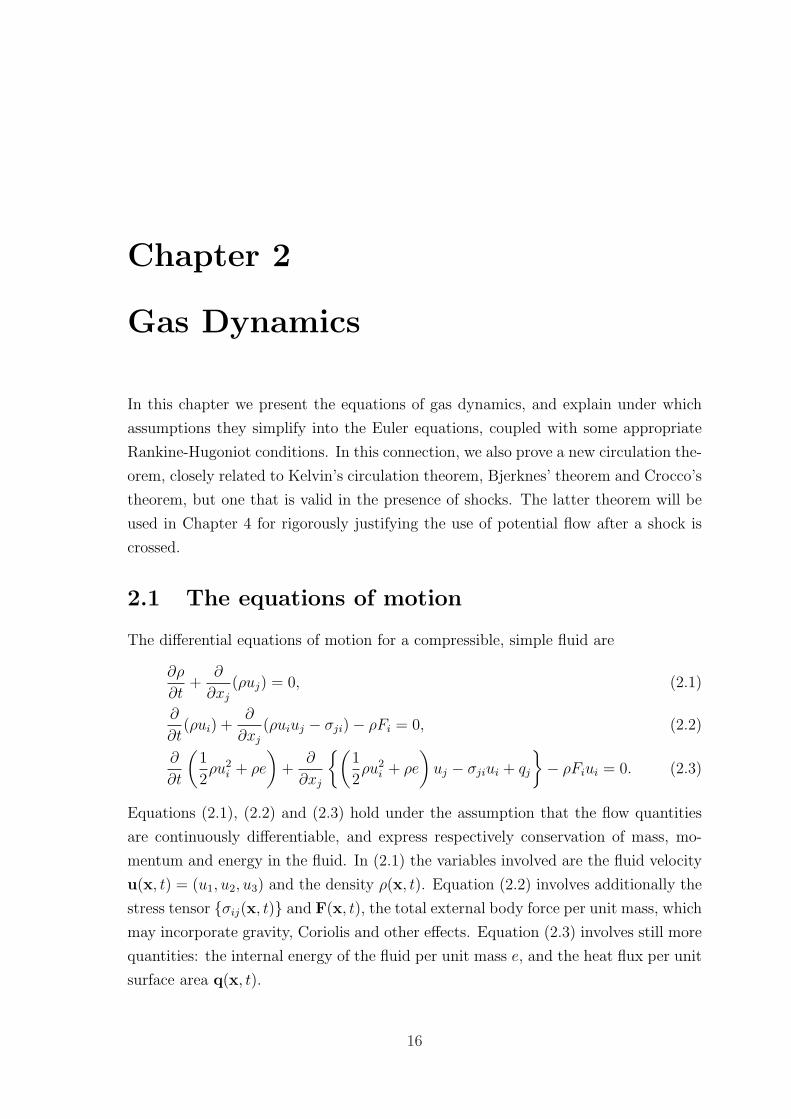
Gas Dynamics
In this chapter we present the equations of gas dynamics, and explain under which
assumptions they simplify into the Euler equations, coupled with some appropriate
Rankine-Hugoniot conditions. In this connection, we also prove a new circulation the-
orem, closely related to Kelvin’s circulation theorem, Bjerknes’ theorem and Crocco’s
theorem, but one that is valid in the presence of shocks. The latter theorem will be
used in Chapter 4 for rigorously justifying the use of potential flow after a shock is
crossed.
2.1 The equations of motion
The differential equations of motion for a compressible, simple fluid are
∂ρ
∂t+
∂
∂xj(ρuj) = 0, (2.1)
∂
∂t(ρui) +
∂
∂xj(ρuiuj − σji)− ρFi = 0, (2.2)
∂
∂t
(1
2ρu2
i + ρe
)+
∂
∂xj
{(1
2ρu2
i + ρe
)uj − σjiui + qj
}− ρFiui = 0. (2.3)
Equations (2.1), (2.2) and (2.3) hold under the assumption that the flow quantities
are continuously differentiable, and express respectively conservation of mass, mo-
mentum and energy in the fluid. In (2.1) the variables involved are the fluid velocity
u(x, t) = (u1, u2, u3) and the density ρ(x, t). Equation (2.2) involves additionally the
stress tensor {σij(x, t)} and F(x, t), the total external body force per unit mass, which
may incorporate gravity, Coriolis and other effects. Equation (2.3) involves still more
quantities: the internal energy of the fluid per unit mass e, and the heat flux per unit
surface area q(x, t).
16
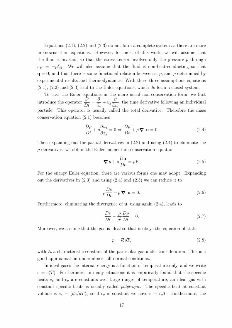
Equations (2.1), (2.2) and (2.3) do not form a complete system as there are more
unknowns than equations. However, for most of this work, we will assume that
the fluid is inviscid, so that the stress tensor involves only the pressure p through
σij = −pδij. We will also assume that the fluid is non-heat-conducting so that
q = 0, and that there is some functional relation between e, p, and ρ determined by
experimental results and thermodynamics. With these three assumptions equations
(2.1), (2.2) and (2.3) lead to the Euler equations, which do form a closed system.
To cast the Euler equations in the more usual non-conservation form, we first
introduce the operatorD
Dt=
∂
∂t+ uj
∂
∂xj, the time derivative following an individual
particle. This operator is usually called the total derivative. Therefore the mass
conservation equation (2.1) becomes
Dρ
Dt+ ρ
∂uj∂xj
= 0 ⇒ Dρ
Dt+ ρ∇ .u = 0. (2.4)
Then expanding out the partial derivatives in (2.2) and using (2.4) to eliminate the
ρ derivatives, we obtain the Euler momentum conservation equation
∇ p+ ρDu
Dt= ρF. (2.5)
For the energy Euler equation, there are various forms one may adopt. Expanding
out the derivatives in (2.3) and using (2.4) and (2.5) we can reduce it to
ρDe
Dt+ p∇ .u = 0. (2.6)
Furthermore, eliminating the divergence of u, using again (2.4), leads to
De
Dt− p
ρ2
Dρ
Dt= 0. (2.7)
Moreover, we assume that the gas is ideal so that it obeys the equation of state
p = RρT, (2.8)
with R a characteristic constant of the particular gas under consideration. This is a
good approximation under almost all normal conditions.
In ideal gases the internal energy is a function of temperature only, and we write
e = e(T ). Furthermore, in many situations it is empirically found that the specific
heats cp and cv are constants over large ranges of temperature; an ideal gas with
constant specific heats is usually called polytropic. The specific heat at constant
volume is cv = (de/dT )v so if cv is constant we have e = cvT . Furthermore, the
17
specific heat at constant pressure is cp = (dh/dT )p, where h = e+p/ρ is the enthalpy
per unit mass, and if cp is constant we have h = cpT . Therefore for a polytropic gas
e and h are both linear functions of temperature. From p/ρ = h − e = (cp − cv)T
and (2.8) we have R = (cp − cv), and it is also customary to define1 γ = cp/cv (see
Whitham [126], p.153). Therefore (2.7) becomes
0 =De
Dt− p
ρ2
Dρ
Dt=
cvRρ
Dp
Dt−
(cvp
Rρ2+
p
ρ2
)Dρ
Dt, (2.9)
=cvRρ
(Dp
Dt− γp
ρ
Dρ
Dt
), (2.10)
= cvTD
Dt
(log
p
ργ
). (2.11)
Letting S = cv logp
ργ+ S0, where S0 is a constant, (2.11) takes the simple form
DS
Dt= 0, (2.12)
where S is the entropy per unit mass, that arises in thermodynamics. Equation (2.12)
states that S remains constant following a fluid particle. Flows that satisfy (2.12) are
usually called isentropic. Furthermore, equation (2.12) can be recast in the simpler
form
pρ−γ = κ = constant, for a fluid particle. (2.13)
If additionally the entropy of every fluid particle is the same, S = S0 thoughout the
flow and the flow is called homentropic.
Finally, equation (2.10) shows that we can write (2.6) as
Dp
Dt= c2
Dρ
Dt, (2.14)
where
c(p, ρ) =
√γp
ρ=
√γRT (2.15)
is the speed of sound with which sound waves propagate relative to the local fluid
velocity u (see Whitham [126], pp. 161–163). In the rest of this thesis we will be
using the latter form of the energy equation.
1For the air under everyday conditions γ is approximately equal to 1.4.
18
2.2 Rankine-Hugoniot conditions
In supersonic flows, discontinuities such as shocks or vortex sheets2 arise and the
Euler differential equations presented above do not hold on them. They need to be
interpreted in the sense of distribution theory or replaced by an equivalent integral
formulation which directly represents the physical laws. The integral formulation is
derived by considering a fixed arbitrary volume occupied by the fluid, V , with surface
S, and writing down the net balance for mass, momentum and energy for that region;
a detailed derivation can be found in most gas dynamics books (see, for instance,
Ockendon and Ockendon [82], Chapter 2) so we do not pursue it here. Even though
the partial differential equations above are derived from an integral formulation we
presented them as differential equations first, since in most of this work we will be
using them rather than the integral formulation. For the Euler equations the integral
formulation is
d
dt
∫
VρdV +
∫
Sρu.dS = 0, (2.16)
d
dt
∫
VρudV +
∫
Sρu(u.dS) +
∫
SpdS =
∫
VρFdV , (2.17)
d
dt
∫
V(ρe+
1
2ρu2)dV +
∫
S
(ρe+
1
2ρu2
)u.dS +
∫
Spu.ndS =
∫
Vρu.FdV . (2.18)
From these integral equations we can deduce the correct relations for the jump of
the flow quantities across a discontinuity. These relations are called the Rankine-
Hugoniot (R-H) conditions; for the derivation see, for instance, Chapman [21], pp.
10–18. We consider a surface of discontinuity with velocity V and normal n where
V is taken to be parallel to n. The R-H conditions, corresponding respectively to
(2.16), (2.17), and (2.18), are
[ρ(u−V).n] = 0, (2.19)
[ρu(u−V).n] = −[pn], (2.20)
[ρ(e+1
2u2)(u−V).n] = −[pu.n], (2.21)
where [...] denotes a jump across the discontinuity. Note that V appears in
(2.19)–(2.21) only through V.n, and from now on we let V.n = V . Also, note
that the external force F does not appear in (2.19)–(2.21).
We first consider shock discontinuities. Shocks have non-zero mass flow across
them and hence the relation ρ(u.n−V ) 6= 0 holds. We can then subtract from (2.21)
2A vortex sheet can also be called a contact discontinuity.
19
the scalar product of V with equation (2.20), and use (2.19) to re-express the energy
R-H condition (2.21) as [e+
p
ρ+
(u−V)2
2
]= 0. (2.22)
We deduce from (2.22) that the total head
H = e+p
ρ+
u2
2+ ψ (2.23)
is conserved across a stationary shock for which V = 0. The symbol ψ is for the po-
tential associated with an external conservative force F = −∇ψ (note that [ψ] = 0).
From (2.20) it follows that u × n, the component of the fluid velocity tangential to
the shock surface, is continuous across the shock (see, for instance, Chapman [21],
pp. 85–87).
The R-H conditions do not determine the flow pattern uniquely. From the second
law of thermodynamics the entropy can only increase when a particle crosses a shock;
it is only by imposing this additional entropy condition that uniqueness can be ensured
(see, for instance, Ockendon and Tayler [84], p. 84).
For vortex sheets, since there is no mass flow across, we have ρ(u.n − V ) = 0.
Therefore the normal component of the velocity u.n is continuous, and the left-hand
side of (2.20) is zero. Consequently the right-hand side gives that the pressure is
continuous across the vortex sheet. Furthermore, equation (2.21) is automatically
satisfied. The equations do not give any information about the jump in the tangential
velocity u × n across the vortex sheet, so this jump is arbitrary. Also, for the same
reason, no entropy condition is necessary and arbitrary values of the entropy may be
taken at the two sides of the sheet.
2.3 Crocco’s equation
Below, we derive Crocco’s equation for a smooth, unsteady flow in an ideal gas
∇H = −∂u∂t
+ u× ω + T ∇S, (2.24)
which is needed in Section 2.4. From the momentum equation (2.5) and the vector
identity
(∇×u)× u = (u.∇)u−∇(
1
2u2
), (2.25)
we have∂u
∂t= −ω × u−∇
(1
2u2
)− ∇ p
ρ+ F. (2.26)
20
Using the thermodynamic relation
TdS = de+ pd(1/ρ) ⇒ TdS = dh− dp
ρ, (2.27)
(see, for instance, Whitham [126]) we can eliminate ∇ p/ρ from (2.26) and deduce
∂u
∂t= −ω × u + T ∇S −∇h−∇
(1
2u2
)+ F. (2.28)
Collecting the ∇ terms together on the left-hand side and using F = −∇ψ, we end
up with equation (2.24) as required.
Note that taking the curl of (2.24) results in the vorticity equation
Dω
Dt= (ω.∇)u− ω(∇ .u) + ∇T ×∇S. (2.29)
2.4 Circulation theorem in a flow with shocks
In a flow with shocks it is important to determine how the amount of the vorticity
produced downstream of a shock is related to the entropy jump at the shock. In the
gas dynamics literature, this question is addressed using Crocco’s equation. However,
Crocco’s equation relates ω×u, the component of vorticity perpendicular to u, to the
entropy gradients in the flow but does not say anything about ω.u, the component
of vorticity parallel to u. The relation of both components of vorticity to the entropy
change can be deduced from a Circulation Theorem, valid in the presence of shocks.
To our knowledge, such a theorem does not exist in the literature so we prove it below
(see also Allwright and Kaouri [8]).
We consider a closed curve C consisting of fluid particles moving with the flow.
The circulation around this closed curve is Γ =
∫
Cu.dx. We assume that there are
shocks in the flow at which the R-H conditions hold and that m of them intersect Ctransversely, at the points Pi(t), 1 ≤ i ≤ m (for a schematic, where four shocks are
shown, see Figure 2.1). The sense of integration in the integral defining Γ and the
order in which we label the shock positions has to be taken the same. In general,
there will be a discontinuity in the tangent to C at each shock position Pi(t).
We now write C =n∑i=1
Ci where Ci is the part of C from Pi to Pi+1, on which the
flow is smooth. The circulation around C is then given by
Γ =n∑i=1
∫
Ci
u.dx =n∑i=1
Γi. (2.30)
21
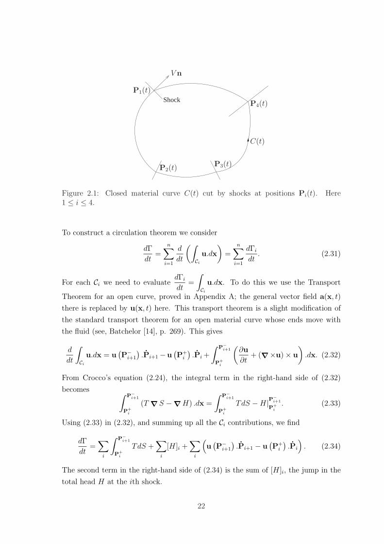
Shock
V n
C(t)
P2(t)P3(t)
P4(t)
P1(t)
Figure 2.1: Closed material curve C(t) cut by shocks at positions Pi(t). Here1 ≤ i ≤ 4.
To construct a circulation theorem we consider
dΓ
dt=
n∑i=1
d
dt
(∫
Ci
u.dx
)=
n∑i=1
dΓidt. (2.31)
For each Ci we need to evaluatedΓidt
=
∫
Ci
u.dx. To do this we use the Transport
Theorem for an open curve, proved in Appendix A; the general vector field a(x, t)
there is replaced by u(x, t) here. This transport theorem is a slight modification of
the standard transport theorem for an open material curve whose ends move with
the fluid (see, Batchelor [14], p. 269). This gives
d
dt
∫
Ci
u.dx = u(P−i+1
).Pi+1−u
(P+i
).Pi +
∫ P−i+1
P+i
(∂u
∂t+ (∇×u)× u
).dx. (2.32)
From Crocco’s equation (2.24), the integral term in the right-hand side of (2.32)
becomes ∫ P−i+1
P+i
(T ∇S −∇H) .dx =
∫ P−i+1
P+i
TdS −H|P−i+1
P+i
. (2.33)
Using (2.33) in (2.32), and summing up all the Ci contributions, we find
dΓ
dt=
∑i
∫ P−i+1
P+i
TdS +∑i
[H]i +∑i
(u
(P−i+1
).Pi+1 − u
(P+i
).Pi
). (2.34)
The second term in the right-hand side of (2.34) is the sum of [H]i, the jump in the
total head H at the ith shock.
22
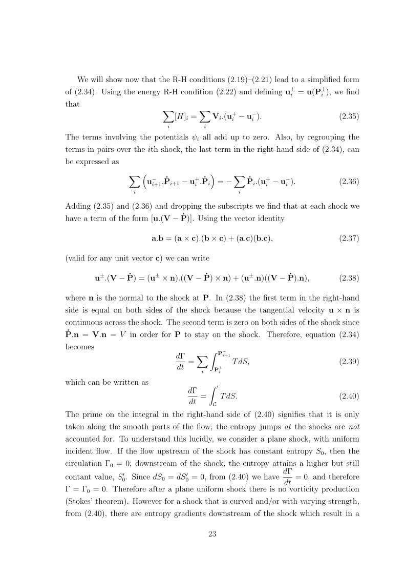
We will show now that the R-H conditions (2.19)–(2.21) lead to a simplified form
of (2.34). Using the energy R-H condition (2.22) and defining u±i = u(P±i ), we find
that ∑i
[H]i =∑i
Vi.(u+i − u−i ). (2.35)
The terms involving the potentials ψi all add up to zero. Also, by regrouping the
terms in pairs over the ith shock, the last term in the right-hand side of (2.34), can
be expressed as
∑i
(u−i+1.Pi+1 − u+
i .Pi
)= −
∑i
Pi.(u+i − u−i ). (2.36)
Adding (2.35) and (2.36) and dropping the subscripts we find that at each shock we
have a term of the form [u.(V − P)]. Using the vector identity
a.b = (a× c).(b× c) + (a.c)(b.c), (2.37)
(valid for any unit vector c) we can write
u±.(V − P) = (u± × n).((V − P)× n) + (u±.n)((V − P).n), (2.38)
where n is the normal to the shock at P. In (2.38) the first term in the right-hand
side is equal on both sides of the shock because the tangential velocity u × n is
continuous across the shock. The second term is zero on both sides of the shock since
P.n = V.n = V in order for P to stay on the shock. Therefore, equation (2.34)
becomesdΓ
dt=
∑i
∫ P−i+1
P+i
TdS, (2.39)
which can be written asdΓ
dt=
∫ ′
CTdS. (2.40)
The prime on the integral in the right-hand side of (2.40) signifies that it is only
taken along the smooth parts of the flow; the entropy jumps at the shocks are not
accounted for. To understand this lucidly, we consider a plane shock, with uniform
incident flow. If the flow upstream of the shock has constant entropy S0, then the
circulation Γ0 = 0; downstream of the shock, the entropy attains a higher but still
contant value, S ′0. Since dS0 = dS ′0 = 0, from (2.40) we havedΓ
dt= 0, and therefore
Γ = Γ0 = 0. Therefore after a plane uniform shock there is no vorticity production
(Stokes’ theorem). However for a shock that is curved and/or with varying strength,
from (2.40), there are entropy gradients downstream of the shock which result in a
23
non-zero value for the circulation, and generally lead to vorticity production. We
remark that for simply connected regions, from Stokes’ theorem, non-zero circulation
leads to non-zero vorticity and vice versa. For multiply connected regions, e.g caused
by an obstruction in the flow, we cannot apply Stokes’ theorem to a curve encircling
the obstruction. It is therefore possible to have non-zero circulation around a material
curve that encircles the obstruction but zero vorticity in the fluid.
One very useful application of the circulation theorem proved above is for weak
shocks, such as those involved in sonic booms. It is well-known that for weak shocks
with strength of order ε, the entropy jump is of order ε3. A general proof of this
is found in Chapman [21], pp. 87–91 for normal shocks in an arbitrary gas3; the
only necessary assumption is that the gas has a convex equation of state, that is
(∂2p/∂v2)S > 0 where v = 1/ρ. Applying (2.40) to any closed material curve in
the incident gas, we conclude that the vorticity in the flow behind a weak shock is
also of order ε3. This result is used in Chapter 4 to justify the use of potential flow
downstream of a shock (up to secobd order in ε). Note that equation (2.40) can also
be used as an additional check on the accuracy of numerical calculations for flows
behind shocks of any strength.
The circulation theorem proved above is an extension of Kelvin’s well-known Cir-
culation theorem for barotropic flows and Bjerknes theorem [16]. Like those theorems,
it is valid for any unsteady flow and can be applied in the presence of obstructions in
the flow (e.g. an aerofoil).
We finally note that it is possible that at a certain instant t = t?, C(t) is tangential
to a shock surface and the number of shocks crossing C in general changes. However
for instantaneous tangencies the circulation Γ is continuous at t?. Therefore, if we
allowdΓ
dt|t?− 6=
dΓ
dt|t?+ equation (2.40) holds for t < t? and t > t?. At vortex sheets,
the problem is more fundamental and the theorem would need modification—see [8].
3In Liepmann and Roshko [70], p. 60 and Whitham [126], p. 176, the same result is proved, butfor the special case of a polytropic gas.
24
Chapter 3
Linear acoustics and ray theory
In this chapter we first give a detailed account of the definitions used in the ray
theory approach to sound propagation, especially as applied to sonic boom problems.
We then solve a series of analytical examples of sound propagation in various model
stratified atmospheres, which help us to clarify aspects of the long-range propagation
of sound, and in particular of secondary boom. Special attention is drawn to the
focusing of rays and boomrays. Where possible we compare our results with the
numerical results for a typical atmopshere.
3.1 Linearised gas dynamics
We start from the Euler equations for unsteady compressible flow (2.4), (2.5) and
(2.10). We shall linearise for small perturbations about an ambient state with pressure
p0(x), density ρ0(x) and flow u0(x). This ambient state must obey the equations
∇ .(ρ0u0) = 0, (3.1)
∇ p0 + ρ0g = 0, (3.2)
u0.(∇ p0 − c2 ∇ ρ0) = 0. (3.3)
We shall make the slightly more restrictive assumption that u0.∇ p0 = 0, so also
u0.∇ ρ0 = 0 and ∇ .u0 = 0. These assumptions hold, for instance, in a gravitation-
ally stratified atmosphere with horizontal wind. Equation (3.2) expresses the fact
that the ambient medium is in hydrostatic equilibrium. From this equation the at-
mospheric length-scale of variation H = P0/(D0g) can be identified, where P0 and D0
are respectively reference pressure and density values. The height H is usually called
the scale height of the atmosphere.
25
In (2.4), (2.5) and (2.10) we set p = p0 + p′, ρ = ρ0 + ρ′ and u = u0 + u′,
where p′ and ρ′ are small compared with the respective ambient values and |u′| ¿ c.
Substituting into (2.4), (2.5) and (2.10) and linearising we obtain
∂ρ′
∂t+ ∇ .(ρ0u
′ + u0ρ′) = 0, (3.4)
ρ0
(∂u′
∂t+ u0.∇u′ + u′.∇u0
)= −∇ p′ − ρ′g, (3.5)
∂p′
∂t+ u0.∇ p′ + u′.∇ p0 = c2
(∂ρ′
∂t+ u0.∇ ρ′ + u′.∇ ρ0
), (3.6)
where c = c(x, y, z) is the local speed of sound in an unperturbed atmosphere. To a
good approximation the air can be considered to be a polytropic gas and therefore
the speed of sound is c =√γp0/ρ0.
We shall see that the system (3.4)–(3.6) sustains acoustic waves, and these will
be our main concern. However, it also sustains gravity waves; a detailed discussion
of the combined theory of these two types of waves appears in Lighthill [72], Section
4.2. Acoustic waves involved in secondary sonic boom (SSB) propagation can be
considered decoupled from internal gravity waves because the latter waves have a
much larger period. The gravity term in the momentum equation (3.5) can therefore
be neglected, even though the ambient pressure p0 varies. (In Chapter 5, where we
consider a moving thin aerofoil in a weakly stratified atmosphere with wind, we will
retain the gravity term but we will show that its effects cancel out in the leading-
order calculation of the wavefield.) Atmospheric gravity waves are however present in
practice, due to normal atmospheric dynamics and these may affect SSB propagation,
but we do not consider them here.1
In sonic boom research, linear acoustics play an important role since a moving thin
aerofoil or a slender body causes only small perturbations to the ambient medium,
and, in many cases, the squares of these perturbations can be assumed to be negligible,
leading thus to a linear problem. The long-range propagation of secondary boom can
be determined to a good approximation by linear theory, and this is what we are
going to concentrate on in this chapter. However, in order to predict the amplitude
of the boom correctly to first order nonlinear effects have to be retained; we shall
discuss this in detail in Chapter 5.
The theory of linear acoustics in a stationary medium is sufficient for investigating
the propagation of thermospheric SSBs and these will be our main concern in this
1Within the SOBER programme, observed atmospheric gravity wave structures were simulated[6] and it was found that these waves indeed alter appreciably some details of SSB propagation [7].
26
chapter. Stratospheric SSBs, occurring only in the presence of wind, will be briefly
considered in Section 3.10, using linear acoustics in moving media.
To examine a stationary medium we now set u0 = 0. We also set g = 0, as justified
by our discussion above. Equations (3.4)–(3.6) can be reduced to a single equation
for pressure. We first use (3.6) to eliminate∂ρ′
∂tfrom (3.4) and then differentiate the
resulting equation with respect to t to get
c−2p′tt + c−2∂u′
∂t.∇ p0 + ρ0 ∇ .
∂u′
∂t= 0. (3.7)
Combining (3.7) and∂u′
∂t= − 1
ρ0∇ p′, obtained from (3.5), multiplying by −c2, and
dropping the dashes, we obtain the second-order wave equation
c2 ∇2 p− ptt +1
ρ0∇ p.(∇ p0 − c2 ∇ ρ0) = 0. (3.8)
The wavelength of the perturbations is of the order of the body length L, which is
around 10 m for a wing and around 100 m for the fuselage. Furthermore, for a typical
atmosphere H is around 8 km. We can thus define a small parameter δ = L/H
which is of order 10−3 for a wing, and of order 10−2 for the fuselage. We will non-
dimensionalise equation (3.8) using x = Lx, p = P0p(z), ρ = D0ρ(z), c = C0c, where
z = z/H = δz and C0 =√γP0/D0. We also take t =
L
C0
t. We obtain
c2∇2p− ptt +
δ
ρ0∇p.(
1
γ∇p0 − c2∇ρ0) = 0, (3.9)
where ∇ denotes differentiation with respect to x, and ∇ denotes differentiation with
respect to z. Since δ is small, at leading order in δ we drop the terms involving the
gradients of p0 and ρ0, and we obtain the wave equation
c2(z)∇2p− ptt = 0. (3.10)
In this form, we are looking for order 1 wavelengths in a slowly varying medium.
Alternatively, we can divide (3.10) by δ2, and let t = δt, x = δx, and then (dropping
the tildes) we have
c2(z) ∇2 p− ptt = 0, (3.11)
where we would be looking for wavelengths of order δ (in a medium with order 1
variations), i.e. large wavenumber solutions.
27
We shall see in Chapter 4 that the wave equation geometry provides a good first
approximation to the position of weak shocks, even though the shocks are an intrin-
sically nonlinear phenomenon. In Chapter 5, where we will address the introduction
of nonlinear effects in a paradigm problem for the prediction of SSB amplitudes, we
will also treat the stratification issue much more fully by retaining the terms of order
δ.
The wave equation is ubiquitous; two fields in which it commonly arises are elastic-
ity and electromagnetism. In electromagnetism, in free space, each component of the
electric field vector E and the magnetic flux density vector B satisfy wave equations
and the speed of light is given by c = 1/√µ0ε0 where ε0 is the electric permittivity
and µ0 the magnetic permeability. In isotropic linear elasticity, the displacement of
a particle from an unstressed reference configuration v(x, t), can be expressed as the
sum of vP = ∇φP and vS = ∇×A where φP and the components of A satisfy wave
equations. (The subscript P stands for primary or pressure waves and the subscript
S for secondary or shear waves.)
We proceed from now on with the paradigm problem of a point impulsive source
at (x0, t0). We do not lose much generality by doing so, as the solution of the wave
equation for an extended body can be expressed as a linear superposition of the
solutions corresponding to such point sources.
A surface ψ = 0 is a characteristic surface of (3.11) if it obeys the eikonal equation
(see Ockendon et al. [85])
c2|∇ψ|2 = ψ2t . (3.12)
(Note that here and for some time we will consider c = c(x) in order to give a
more general exposition; we return to stratified media in Section 3.3.) We assume
of course that ψ = 0 is a non-singular representation of the surface, so ∇ψ and
ψt do not vanish. When (3.12) is solved by Charpit’s method [85], the trajectories
passing through the source at (x0, t0), called bicharacteristics, are the curves on which
information propagates [85, 21]. Bicharacteristics form a particular characteristic
surface of (3.11), called the ray conoid through (x0, t0). The part of the ray conoid
in t > t0 is the boundary of the region of influence of (x0, t0), and the part in t < t0
is the boundary of its dependence domain.
In order to solve equation (3.12), we recast it in the form
F =1
2
(ψt − c2
ψt(ψ2
x + ψ2y + ψ2
z)
)= 0. (3.13)
28
Letting p = ψx, q = ψy, r = ψz, λ = ψt, equation (3.13) becomes
F =1
2
(λ− c2
λ(p2 + q2 + r2)
)= 0. (3.14)
(Note that p no longer represents the pressure.) Charpit’s method reduces the non-
linear partial differential equation (PDE) to a system of eight ordinary differential
equations which yield the bicharacteristics. Bicharacteristics are also frequently called
rays and from now on when we refer to rays it will be in this context. Also, frequently
the ray conoid may be called ray surface. Charpit’s equations for the coordinates
(x, t) = (x, y, z, t) are
dx
ds=∂F
∂p= −c2 p
λ, (3.15)
dy
ds=∂F
∂q= −c2 q
λ, (3.16)
dz
ds=∂F
∂r= −c2 r
λ, (3.17)
dt
ds=∂F
∂λ=
1
2+
c2
2λ2(p2 + q2 + r2) = 1. (3.18)
When s = s0, (x, t) takes the initial value (x0, t0). Integrating equation (3.18) and
taking s0 = t0 we deduce that s = t. Therefore the parameter along the rays is the
time t, and this is why we use (3.13) instead of (3.12). The remaining four Charpit’s
equations for p, q, r and λ are
dp
ds= −∂F
∂x− p
∂F
∂ψ= cxλ/c, (3.19)
dq
ds= −∂F
∂y− q
∂F
∂ψ= cyλ/c, (3.20)
dr
ds= −∂F
∂z− q
∂F
∂ψ= czλ/c, (3.21)
dλ
ds= −∂F
∂t− r
∂F
∂ψ= 0 ⇒ λ = λ0. (3.22)
In order to be able to solve the system the initial values (p0, q0, r0, λ0) should also be
provided, satisfying (3.14). Equation (3.22) gives that λ is conserved along the rays,
and by rescaling (p, q, r) we can set λ0 = 1. This homogeneity in time arises because
the medium is time-independent and it is also expressed by the relation
ψ(x, t) = t− σ(x). (3.23)
(The choice of λ0 > 0 corresponds to the convention that ψ > 0 behind the surface
and ψ < 0 ahead of it.) The family of surfaces σ(x) = t are the wavefronts. A
29
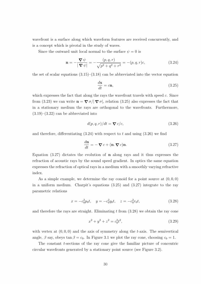
wavefront is a surface along which waveform features are received concurrently, and
is a concept which is pivotal in the study of waves.
Since the outward unit local normal to the surface ψ = 0 is
n = − ∇ψ
|∇ψ| = − (p, q, r)√p2 + q2 + r2
= −(p, q, r)c, (3.24)
the set of scalar equations (3.15)–(3.18) can be abbreviated into the vector equation
dx
dt= cn, (3.25)
which expresses the fact that along the rays the wavefront travels with speed c. Since
from (3.23) we can write n = ∇σ/|∇σ|, relation (3.25) also expresses the fact that
in a stationary medium the rays are orthogonal to the wavefronts. Furthermore,
(3.19)–(3.22) can be abbreviated into
d(p, q, r)/dt = ∇ c/c, (3.26)
and therefore, differentiating (3.24) with respect to t and using (3.26) we find
dn
dt= −∇ c+ (n.∇ c)n. (3.27)
Equation (3.27) dictates the evolution of n along rays and it thus expresses the
refraction of acoustic rays by the sound speed gradient. In optics the same equation
expresses the refraction of optical rays in a medium with a smoothly varying refractive
index.
As a simple example, we determine the ray conoid for a point source at (0, 0, 0)
in a uniform medium. Charpit’s equations (3.25) and (3.27) integrate to the ray
parametric relations
x = −c20p0t, y = −c20q0t, z = −c20r0t, (3.28)
and therefore the rays are straight. Eliminating t from (3.28) we obtain the ray cone
x2 + y2 + z2 = c20t2, (3.29)
with vertex at (0, 0, 0) and the axis of symmetry along the t-axis. The semivertical
angle, β say, obeys tan β = c0. In Figure 3.1 we plot the ray cone, choosing c0 = 1.
The constant t-sections of the ray cone give the familiar picture of concentric
circular wavefronts generated by a stationary point source (see Figure 3.2).
30

Figure 3.1: Ray cone for a uniform medium (c0 = 1), in the (x, z, t) space.
SOURCE
Figure 3.2: Wavefronts generated by a stationary point source in a uniform medium.
31
Note that the use of equations (3.25) and (3.27) for studying the propagation of
sound in non-uniform media did not become established till the 20th century. They
are very useful because, even though generally nonlinear, they are of first order and
thus amenable to standard numerical techniques (see, for instance, the article by
Moler and Solomon [80]). The procedure of determining the rays is frequently called
ray tracing.
3.2 Geometrical Acoustics
The eikonal equation (3.12) also arises at the leading order of the high-frequency
(WKB) approximation to the wave equation. The characteristics of this equation are
also called rays. This is the framework of Geometrical Acoustics (GA). We can use a
high-frequency approximation when the wavelength is much smaller than the charac-
teristic propagation length in the problem. Also for light, where the wavelength is of
order 10−7 m, the high-frequency approximation is often appropriate2, and we refer
to the framework of Geometrical Optics (GO). However, high-frequency approxima-
tions generally need more scrutiny in the case of sound or elastic waves, where the
wavelength can be up to a few metres or kilometres.
Below we outline the GA ansatz, in a medium with an ambient state that is slowly
varying in space. We first let the pressure p = <(A exp(ikΘ)), where k = H/λ is
large, with λ being a typical wavelength of the wave. The amplitude A and the wave
phase Θ are both slowly varying in space and time, in the sense that they vary by
order 1 when x varies by order 1. The terms of order k2 in (3.11) give the eikonal
equation3
Θ2t = c2|∇ Θ|2, (3.30)
which leads to the same bicharacteristics as those of the hyperbolic PDE framework
presented above. Since the phase for a plane wave is Θ = k.r− ωt we may define in
general
k = ∇ Θ, ω = −∂Θ
∂t, (3.31)
2except in optical fibres, photonic crystals, and so on3Note that the term “eikonal” was introduced in optics by Bruns in 1895 but the concept was
already known by Hamilton in 1832. The eikonal equation applicable to propagation of weak acousticdiscontinuities was derived by Heller in 1953 [56] and by Keller in 1954 [65]. These derivations werefor the more general case of acoustics in moving media.
32
so that k is the wavevector and ω the frequency. Therefore the eikonal equation (3.30)
becomes
ω2 = c2|k|2, (3.32)
which is the dispersion relation for (3.11).
The word “ray” is somewhat ambiguous in sonic boom literature. We have seen
above two uses of this word; in the hyperbolic PDE framework and in the GA frame-
work. Furthermore, an acoustic ray may also stand for the stationary time path of
sound just as an optical ray is the stationary path for light. According to this third
definition, a ray obeys Fermat’s principle.4 The rays obtained by GA comply with
Fermat’s principle but the latter principle is more general than GA and can also cater
for diffraction phenomena (see Pierce [94], p. 248). Finally, boomrays are also usually
called rays in the sonic boom literature; these will be discussed in detail in Section
3.4.2.
3.3 Stratified media and Snell’s law
To a first approximation we can assume that the atmosphere is stratified in the vertical
direction, so that the local sound speed profile is a function only of the height z, that
is c(x) = c(z). This is in fact an assumption made throughout this thesis, wherever
we consider non-uniform media. Charpit’s equations (3.15)–(3.22) simplify then to
dx
dt= −c2(z)p0,
dy
dt= −c2(z)q0, dz
dt= −c2(z)r, (3.33)
p = p0, q = q0,dr
dt=czc. (3.34)
Equations (3.33)–(3.34) show that only r changes with height, and therefore any ray
remains in the same vertical plane in which it starts. Since we can always find a
coordinate system such that q0 = 0, it is sufficient to pursue only a two-dimensional
analysis, with x the horizontal coordinate and z the vertical coordinate. Let θ be the
angle a ray makes with the positive x-axis. From (3.33) we have cos θ =1
c
dx
dt= −cp0,
and since p0 is constant, we obtain
c(z)
cos θ=
c0cos θ0
. (3.35)
4Fermat conjectured in 1657 that optical rays are least-time paths. It was Hamilton in 1833 whorealised and postulated that they are in fact stationary-time paths with respect to the time of travelin adjacent ray paths. More than one century later (1972) Ugincius proved that the latter principleholds also for acoustic rays in moving media.
33
This is Snell’s law, known to govern the propagation of optical rays in media where
the refractive index may vary in the vertical direction. For propagation of sound
in a stationary medium, Snell’s law is equivalent to p and q being constant. In
Section 3.10 we show that the latter is also true for stratified media with horizontal
wind. Furthermore, from the first and third equations in (3.33), and using the eikonal
equation c2(p20 + r2) = 1 to express r in terms of p0, we find
dz
dx= ± r
p0
= ± 1
p0
√1
c2− p2
0. (3.36)
Since p0 = − cos θ0/c0, we find that a ray launched at (x0, z0) obeys the ray integral
x− x0 = ±∫ z
z0
c(z) cos θ0/c0√1− c2(z) cos2 θ0/c20
dz, (3.37)
where the ± corresponds to upwards/downwards launching of the ray. The ray inte-
gral (3.37) provides an alternative way to calculate rays in stratified media; we can
perform the single quadrature on the right-hand side rather than solve the system
of Charpit’s equations (3.33)–(3.34). However the denominator of (3.37) has a sin-
gularity at the turning points of the rays where cos θ = c(z) cos θ0/c0 = 1; it is thus
preferable to deal directly with the ordinary differential equations if turning points
are involved.
3.4 The Mach envelope
Let us now consider a moving point source, in a stationary, possibly non-uniform,
medium. We denote the displacement of the source by x0(t) and its velocity by
U(t) = x0(t). We also denote by c0(x0(t), t) the sound speed at the source position.
We define the Mach number of the source as M0 = |U|/c0. For a source moving
supersonically we have M0 > 1 and for a source moving subsonically we have M0 < 1.
3.4.1 Mach envelope as envelope of ray conoids
A supersonic source moves faster than the waves it generates and the ray conoids form
an envelope, called the Mach envelope.5 If we represent the ray conoid emanating
from (x0(τ), τ) by ψ(x, y, z, t; τ) = 0, so that τ is the conoid label, the envelope is
determined as a function of x, y, z, and t by eliminating τ from the equations
ψ = 0 and∂ψ
∂τ= 0. (3.38)
5For motions that are supersonic for only part of the time, e.g. acceleration through the soundspeed, an envelope is formed only by the supersonic part of the motion (see Chapter 6).
34
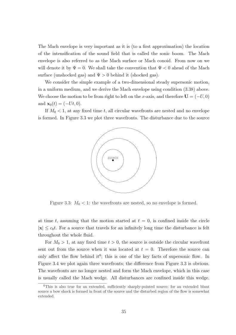
The Mach envelope is very important as it is (to a first approximation) the location
of the intensification of the sound field that is called the sonic boom. The Mach
envelope is also referred to as the Mach surface or Mach conoid. From now on we
will denote it by Ψ = 0. We shall take the convention that Ψ < 0 ahead of the Mach
surface (unshocked gas) and Ψ > 0 behind it (shocked gas).
We consider the simple example of a two-dimensional steady supersonic motion,
in a uniform medium, and we derive the Mach envelope using condition (3.38) above.
We choose the motion to be from right to left on the x-axis, and therefore U = (−U, 0)
and x0(t) = (−Ut, 0).
If M0 < 1, at any fixed time t, all circular wavefronts are nested and no envelope
is formed. In Figure 3.3 we plot three wavefronts. The disturbance due to the source
SOURCE
Figure 3.3: M0 < 1: the wavefronts are nested, so no envelope is formed.
at time t, assuming that the motion started at t = 0, is confined inside the circle
|x| ≤ c0t. For a source that travels for an infinitely long time the disturbance is felt
throughout the whole fluid.
For M0 > 1, at any fixed time t > 0, the source is outside the circular wavefront
sent out from the source when it was located at t = 0. Therefore the source can
only affect the flow behind it6; this is one of the key facts of supersonic flow. In
Figure 3.4 we plot again three wavefronts; the difference from Figure 3.3 is obvious.
The wavefronts are no longer nested and form the Mach envelope, which in this case
is usually called the Mach wedge. All disturbances are confined inside this wedge.
6This is also true for an extended, sufficiently sharply-pointed source; for an extended bluntsource a bow shock is formed in front of the source and the disturbed region of the flow is somewhatextended.
35
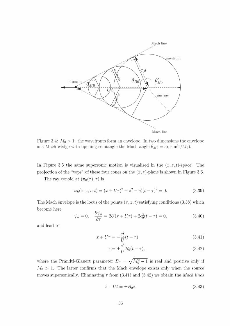
����
c0t
Ut
SOURCE
Mach line
Mach line
wavefront
any ray
θB0 θ′B0
boo
mra
yboom
ray
θM0
Figure 3.4: M0 > 1: the wavefronts form an envelope. In two dimensions the envelopeis a Mach wedge with opening semiangle the Mach angle θM0 = arcsin(1/M0).
In Figure 3.5 the same supersonic motion is visualised in the (x, z, t)-space. The
projection of the “tops” of these four cones on the (x, z)-plane is shown in Figure 3.6.
The ray conoid at (x0(τ), τ) is
ψh(x, z, τ ; t) = (x+ Uτ)2 + z2 − c20(t− τ)2 = 0. (3.39)
The Mach envelope is the locus of the points (x, z, t) satisfying conditions (3.38) which
become here
ψh = 0,∂ψh∂τ
= 2U(x+ Uτ) + 2c20(t− τ) = 0, (3.40)
and lead to
x+ Uτ = −c20
U(t− τ), (3.41)
z = ±c20
UB0(t− τ), (3.42)
where the Prandtl-Glauert parameter B0 =√M2
0 − 1 is real and positive only if
M0 > 1. The latter confirms that the Mach envelope exists only when the source
moves supersonically. Eliminating τ from (3.41) and (3.42) we obtain the Mach lines
x+ Ut = ±B0z. (3.43)
36
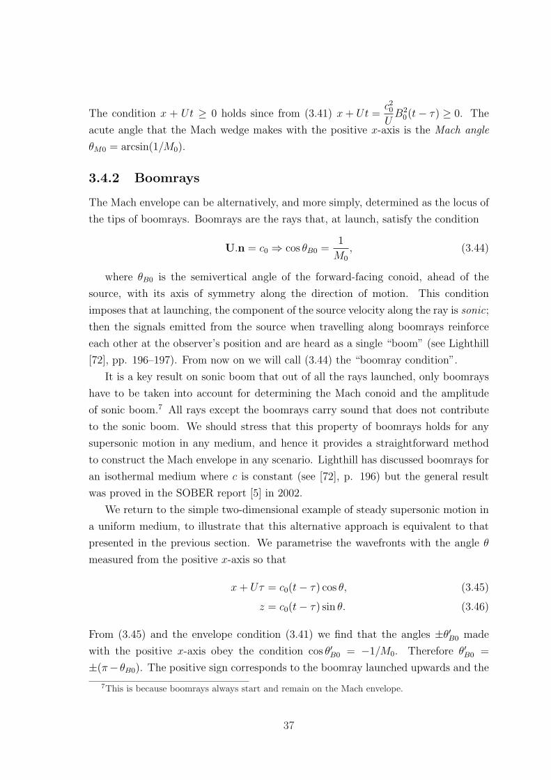
The condition x + Ut ≥ 0 holds since from (3.41) x+ Ut =c20UB2
0(t− τ) ≥ 0. The
acute angle that the Mach wedge makes with the positive x-axis is the Mach angle
θM0 = arcsin(1/M0).
3.4.2 Boomrays
The Mach envelope can be alternatively, and more simply, determined as the locus of
the tips of boomrays. Boomrays are the rays that, at launch, satisfy the condition
U.n = c0 ⇒ cos θB0 =1
M0
, (3.44)
where θB0 is the semivertical angle of the forward-facing conoid, ahead of the
source, with its axis of symmetry along the direction of motion. This condition
imposes that at launching, the component of the source velocity along the ray is sonic;
then the signals emitted from the source when travelling along boomrays reinforce
each other at the observer’s position and are heard as a single “boom” (see Lighthill
[72], pp. 196–197). From now on we will call (3.44) the “boomray condition”.
It is a key result on sonic boom that out of all the rays launched, only boomrays
have to be taken into account for determining the Mach conoid and the amplitude
of sonic boom.7 All rays except the boomrays carry sound that does not contribute
to the sonic boom. We should stress that this property of boomrays holds for any
supersonic motion in any medium, and hence it provides a straightforward method
to construct the Mach envelope in any scenario. Lighthill has discussed boomrays for
an isothermal medium where c is constant (see [72], p. 196) but the general result
was proved in the SOBER report [5] in 2002.
We return to the simple two-dimensional example of steady supersonic motion in
a uniform medium, to illustrate that this alternative approach is equivalent to that
presented in the previous section. We parametrise the wavefronts with the angle θ
measured from the positive x-axis so that
x+ Uτ = c0(t− τ) cos θ, (3.45)
z = c0(t− τ) sin θ. (3.46)
From (3.45) and the envelope condition (3.41) we find that the angles ±θ′B0 made
with the positive x-axis obey the condition cos θ′B0 = −1/M0. Therefore θ′B0 =
±(π− θB0). The positive sign corresponds to the boomray launched upwards and the
7This is because boomrays always start and remain on the Mach envelope.
37
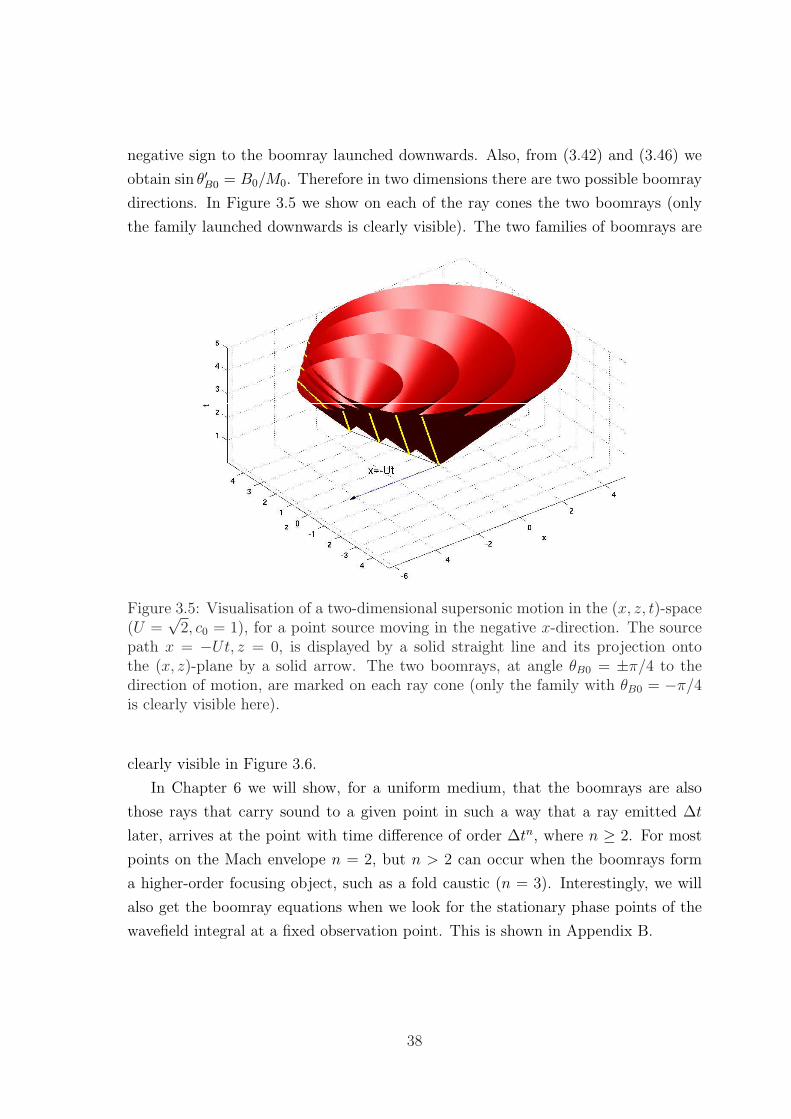
negative sign to the boomray launched downwards. Also, from (3.42) and (3.46) we
obtain sin θ′B0 = B0/M0. Therefore in two dimensions there are two possible boomray
directions. In Figure 3.5 we show on each of the ray cones the two boomrays (only
the family launched downwards is clearly visible). The two families of boomrays are
Figure 3.5: Visualisation of a two-dimensional supersonic motion in the (x, z, t)-space(U =
√2, c0 = 1), for a point source moving in the negative x-direction. The source
path x = −Ut, z = 0, is displayed by a solid straight line and its projection ontothe (x, z)-plane by a solid arrow. The two boomrays, at angle θB0 = ±π/4 to thedirection of motion, are marked on each ray cone (only the family with θB0 = −π/4is clearly visible here).
clearly visible in Figure 3.6.
In Chapter 6 we will show, for a uniform medium, that the boomrays are also
those rays that carry sound to a given point in such a way that a ray emitted ∆t
later, arrives at the point with time difference of order ∆tn, where n ≥ 2. For most
points on the Mach envelope n = 2, but n > 2 can occur when the boomrays form
a higher-order focusing object, such as a fold caustic (n = 3). Interestingly, we will
also get the boomray equations when we look for the stationary phase points of the
wavefield integral at a fixed observation point. This is shown in Appendix B.
38
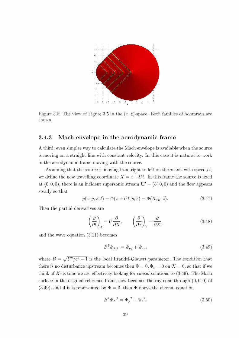
Figure 3.6: The view of Figure 3.5 in the (x, z)-space. Both families of boomrays areshown.
3.4.3 Mach envelope in the aerodynamic frame
A third, even simpler way to calculate the Mach envelope is available when the source
is moving on a straight line with constant velocity. In this case it is natural to work
in the aerodynamic frame moving with the source.
Assuming that the source is moving from right to left on the x-axis with speed U ,
we define the new travelling coordinate X = x+Ut. In this frame the source is fixed
at (0, 0, 0), there is an incident supersonic stream U′ = (U, 0, 0) and the flow appears
steady so that
p(x, y, z, t) = Φ(x+ Ut, y, z) = Φ(X, y, z). (3.47)
Then the partial derivatives are
(∂
∂t
)
x
= U∂
∂X,
(∂
∂x
)
t
=∂
∂X, (3.48)
and the wave equation (3.11) becomes
B2ΦXX = Φyy + Φzz, (3.49)
where B =√U2/c2 − 1 is the local Prandtl-Glauert parameter. The condition that
there is no disturbance upstream becomes then Φ = 0,Φx = 0 on X = 0, so that if we
think of X as time we are effectively looking for causal solutions to (3.49). The Mach
surface in the original reference frame now becomes the ray cone through (0, 0, 0) of
(3.49), and if it is represented by Ψ = 0, then Ψ obeys the eikonal equation
B2ΨX2 = Ψy
2 + Ψz2. (3.50)
39
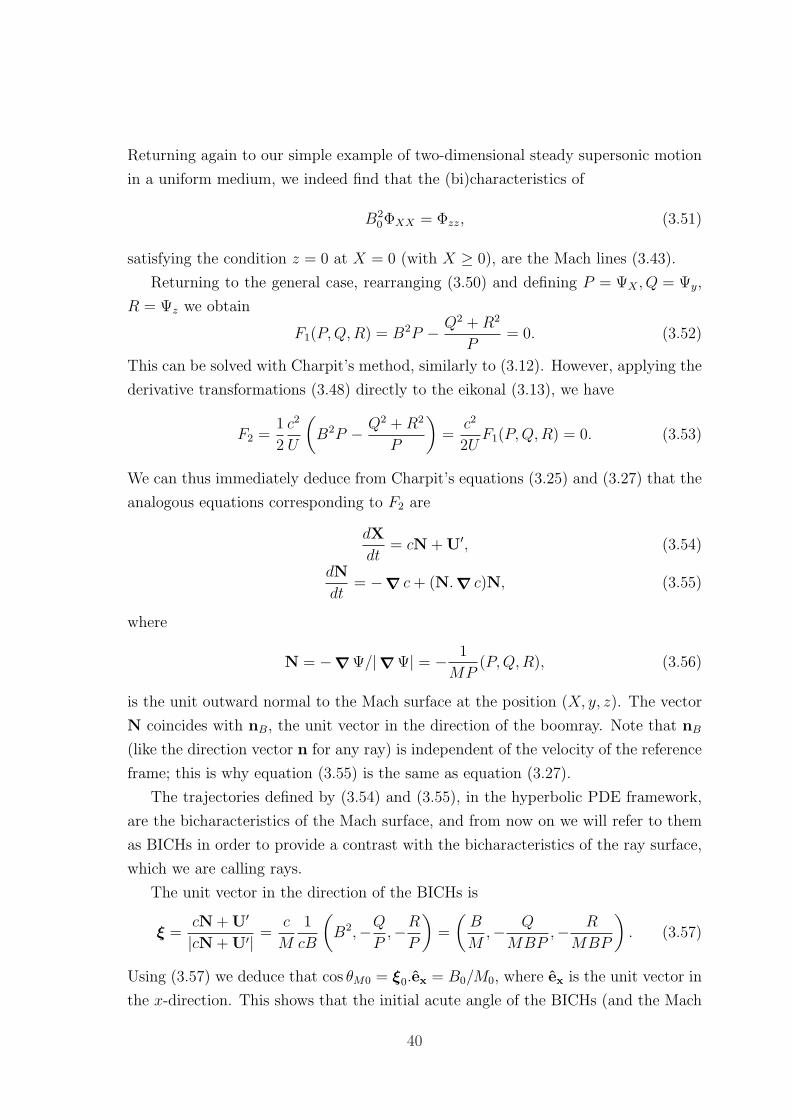
Returning again to our simple example of two-dimensional steady supersonic motion
in a uniform medium, we indeed find that the (bi)characteristics of
B20ΦXX = Φzz, (3.51)
satisfying the condition z = 0 at X = 0 (with X ≥ 0), are the Mach lines (3.43).
Returning to the general case, rearranging (3.50) and defining P = ΨX , Q = Ψy,
R = Ψz we obtain
F1(P,Q,R) = B2P − Q2 +R2
P= 0. (3.52)
This can be solved with Charpit’s method, similarly to (3.12). However, applying the
derivative transformations (3.48) directly to the eikonal (3.13), we have
F2 =1
2
c2
U
(B2P − Q2 +R2
P
)=
c2
2UF1(P,Q,R) = 0. (3.53)
We can thus immediately deduce from Charpit’s equations (3.25) and (3.27) that the
analogous equations corresponding to F2 are
dX
dt= cN + U′, (3.54)
dN
dt= −∇ c+ (N.∇ c)N, (3.55)
where
N = −∇ Ψ/|∇ Ψ| = − 1
MP(P,Q,R), (3.56)
is the unit outward normal to the Mach surface at the position (X, y, z). The vector
N coincides with nB, the unit vector in the direction of the boomray. Note that nB
(like the direction vector n for any ray) is independent of the velocity of the reference
frame; this is why equation (3.55) is the same as equation (3.27).
The trajectories defined by (3.54) and (3.55), in the hyperbolic PDE framework,
are the bicharacteristics of the Mach surface, and from now on we will refer to them
as BICHs in order to provide a contrast with the bicharacteristics of the ray surface,
which we are calling rays.
The unit vector in the direction of the BICHs is
ξ =cN + U′
|cN + U′| =c
M
1
cB
(B2,−Q
P,−R
P
)=
(B
M,− Q
MBP,− R
MBP
). (3.57)
Using (3.57) we deduce that cos θM0 = ξ0.ex = B0/M0, where ex is the unit vector in
the x-direction. This shows that the initial acute angle of the BICHs (and the Mach
40

conoid) with the positive x-axis is the Mach angle θM0 = arcsin(1/M0), as expected.
More generally, at any height the BICH is at the local Mach angle to the x-axis,
θM = arcsin(1/M), since cos θM = ξ.ex = B/M . Furthermore, the BICH passing
through any position (X, y, z) is perpendicular to the boomray since the dot product
of ξ with N is ξ.N =c+ U′.N|cN + U′| = 0.
In the aerodynamic frame, the causality of the PDE (3.49) dictates that any
information introduced at a certain point will move along the BICHs. To see this
physically take a point X on the Mach conoid. In stationary air, the portion of
the shock front centered on X = (X, y, z), would advance a distance cNδt in time
δt. However, in the aerodynamic frame, within the same time interval, the incident
supersonic stream U′ = (U, 0, 0) sweeps the shock front portion horizontally to the
right by distance Uδt. Therefore the new position of the shock front portion is
X + δX = X + (cN + (U, 0, 0))δt which leads to the equation (3.54), as required.
Equivalently, we can say that for a stationary observer the perceived direction of
propagation is along the boomray, but for an observer moving with the source the
perceived direction of propagation is along the BICH. Note that by construction the
parameter along the BICHs is still the time t.
Up to now, we have presented three ways to derive the Mach envelope and illus-
trated each one with the two-dimensional example of a source with constant super-
sonic speed in a uniform atmosphere. For the latter example, extension into three
dimensions is trivial: the wavefronts are spheres (t-sections of the ray cone (3.29)),
the boomrays lie on the cone with semivertical angle θB0, ahead of the source position
and the BICHS lie on the Mach cone
(x+ Ut)2 = B20(y
2 + z2), (3.58)
which can also be found as the ray cone of B20ΦXX = Φyy + Φzz, or as the body
of revolution with the Mach lines (3.43) as its generators. However, for a general
scenario of unsteady motion in an non-uniform medium the Mach envelope cannot,
in most cases, be determined analytically. Below we pinpoint some examples where
this is possible, with the aim of elucidating sonic boom propagation.
3.5 Stationary source in a model stratified atmo-
sphere (two dimensions)
For a second analytical example, we consider a stratified medium with sound speed
profile c =1√
1− zin the region z < 1. Even though this profile has an unphysical
41
singularity at z = 1, where the speed of sound becomes infinite, we can take it as
a representation of cases where c(z) is increasing with height. Perhaps the simplest
analytical example of a stratified medium that we could have taken is one with c
varying linearly with z. The rays are then arcs of circles ([94], p. 385), and the
dependence on the independent coordinates x, y, z, t appears through trigonometric
functions. However, for the example here the Mach envelope will be determined as
a polynomial in x, y, z, t, which makes the analysis easier. At the same time, this
example gives rise to a quite complicated geometry with features that are relevant
physically.
The analysis that we will present here for the stationary source will become directly
relevant to the three-dimensional scenario with B2 = 1 − z with just a coordinate
change.8 Note that the scenario with B2 = 1− z can be thought of as the canonical
problem for the approximation of B near the reflection height in any atmosphere.
For a stationary source at (0, 0, 0) we derive below the ray conoid. Since the
propagation vector remains in the plane in which it originates, it is sufficient to
remain in two spatial dimensions. Equation (3.11) becomes
(1− z)ptt = pxx + pzz. (3.59)
Writing the eikonal equation (3.12) in the form
F3 = (1− z)λ2 − (p2 + r2) = 0 (3.60)
will enable us to determine the ray conoid analytically. Charpit’s equations for (3.60)
integrate to the following parametric relations for the rays,
x(ζ) = −2p0ζ, (3.61)
z(ζ) = −λ20ζ
2 − 2r0ζ, (3.62)
t(ζ) =2
3λ3
0ζ3 + 2λ0r0ζ
2 + 2λ0ζ, (3.63)
p = p0, r(ζ) = λ20ζ + r0, λ = λ0. (3.64)
(Equations (3.61)–(3.64) also appear in [86], p. 389.) Note that we do not take
λ0 = 1 because later on (Section 3.8) we will use equations (3.61)–(3.64), under the
coordinate transformation (x, z, t) → (y, z,X), for directly determining the Mach
surface in the three-dimensional scenario with B2 = 1 − z. There λ0 is associated
with the X coordinate and cannot be taken equal to 1.
8Furthermore the analysis for B2 = 1 − z will pave the way for solving analytically the morecomplicated scenario B2 = 1 − |z|, which provides a good insight into the geometry of the Machenvelope in a typical atmosphere, where calculations can only be done numerically—see Section 3.8.
42
The parameter along the rays is no longer the time t but we can readily see that∂t
∂ζ= 2λ0(1− z) > 0 (assuming λ0 > 0). Therefore the time t increases monotonically
with ζ and the qualitative behaviour of the ray will not be affected by using the
parameter ζ instead of t.
To determine the ray conoid as an algebraic relation between x, z and t, we need to
eliminate ζ, p0, r and λ0 from the equations (3.61)–(3.64). (We will study graphically
the latter equations later.) From equation (3.61) we solve for ζ = −x/(2p0) and
substitute into (3.62) and (3.63). We obtain respectively
z = −1
4
(λ0
p0
)2
x2 +
(r0p0
)x, (3.65)
t = − 1
12
(λ0
p0
)3
x3 +1
2
(λ0
p0
)(r0p0
)x2 −
(λ0
p0
)x. (3.66)
Because of the eikonal equation (3.60), the dimensionless ratiosλ0
p0
andr0p0
satisfy
(λ0
p0
)2
= 1 +
(r0p0
)2
. (3.67)
Letting C =λ0
p0
and D =r0p0
, we can write (3.65)–(3.67) as a system of three algebraic
equations linked through the two parameters C and D:
C2 = 1 +D2, (3.68)
z = −1
4(Cx)2 +Dx, (3.69)
t = − 1
12(Cx)3 +
1
2CDx2 − Cx. (3.70)
From equation (3.69) we find D(x, z, C), substitute in (3.68), rearrange and we get a
quadratic in (Cx)2,
(Cx)4 + (Cx)2(8z − 16) + 16(x2 + z2) = 0, (3.71)
which gives the roots
1
4(Cx)2 = (2− z)±
√4(1− z)− x2. (3.72)
For the two roots to be real, we need to impose the constraint z ≤ 1 − x2/4, which
indicates a qualitative change in the behaviour of the wavefield, on the curve
z = 1− x2
4. (3.73)
43
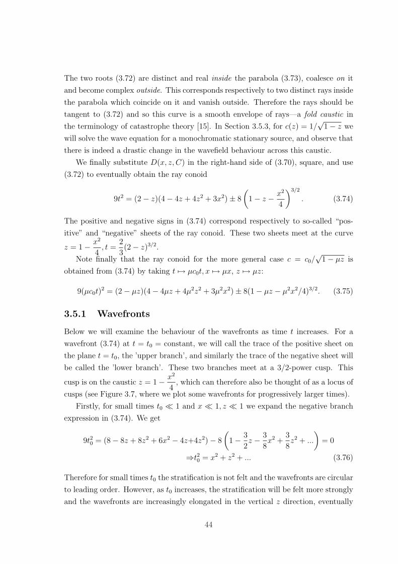
The two roots (3.72) are distinct and real inside the parabola (3.73), coalesce on it
and become complex outside. This corresponds respectively to two distinct rays inside
the parabola which coincide on it and vanish outside. Therefore the rays should be
tangent to (3.72) and so this curve is a smooth envelope of rays—a fold caustic in
the terminology of catastrophe theory [15]. In Section 3.5.3, for c(z) = 1/√
1− z we
will solve the wave equation for a monochromatic stationary source, and observe that
there is indeed a drastic change in the wavefield behaviour across this caustic.
We finally substitute D(x, z, C) in the right-hand side of (3.70), square, and use
(3.72) to eventually obtain the ray conoid
9t2 = (2− z)(4− 4z + 4z2 + 3x2)± 8
(1− z − x2
4
)3/2
. (3.74)
The positive and negative signs in (3.74) correspond respectively to so-called “pos-
itive” and “negative” sheets of the ray conoid. These two sheets meet at the curve
z = 1− x2
4, t =
2
3(2− z)3/2.
Note finally that the ray conoid for the more general case c = c0/√
1− µz is
obtained from (3.74) by taking t 7→ µc0t, x 7→ µx, z 7→ µz:
9(µc0t)2 = (2− µz)(4− 4µz + 4µ2z2 + 3µ2x2)± 8(1− µz − µ2x2/4)3/2. (3.75)
3.5.1 Wavefronts
Below we will examine the behaviour of the wavefronts as time t increases. For a
wavefront (3.74) at t = t0 = constant, we will call the trace of the positive sheet on
the plane t = t0, the ’upper branch’, and similarly the trace of the negative sheet will
be called the ’lower branch’. These two branches meet at a 3/2-power cusp. This
cusp is on the caustic z = 1− x2
4, which can therefore also be thought of as a locus of
cusps (see Figure 3.7, where we plot some wavefronts for progressively larger times).
Firstly, for small times t0 ¿ 1 and x ¿ 1, z ¿ 1 we expand the negative branch
expression in (3.74). We get
9t20 = (8− 8z + 8z2 + 6x2 − 4z+4z2)− 8
(1− 3
2z − 3
8x2 +
3
8z2 + ...
)= 0
⇒t20 = x2 + z2 + ... (3.76)
Therefore for small times t0 the stratification is not felt and the wavefronts are circular
to leading order. However, as t0 increases, the stratification will be felt more strongly
and the wavefronts are increasingly elongated in the vertical z direction, eventually
44
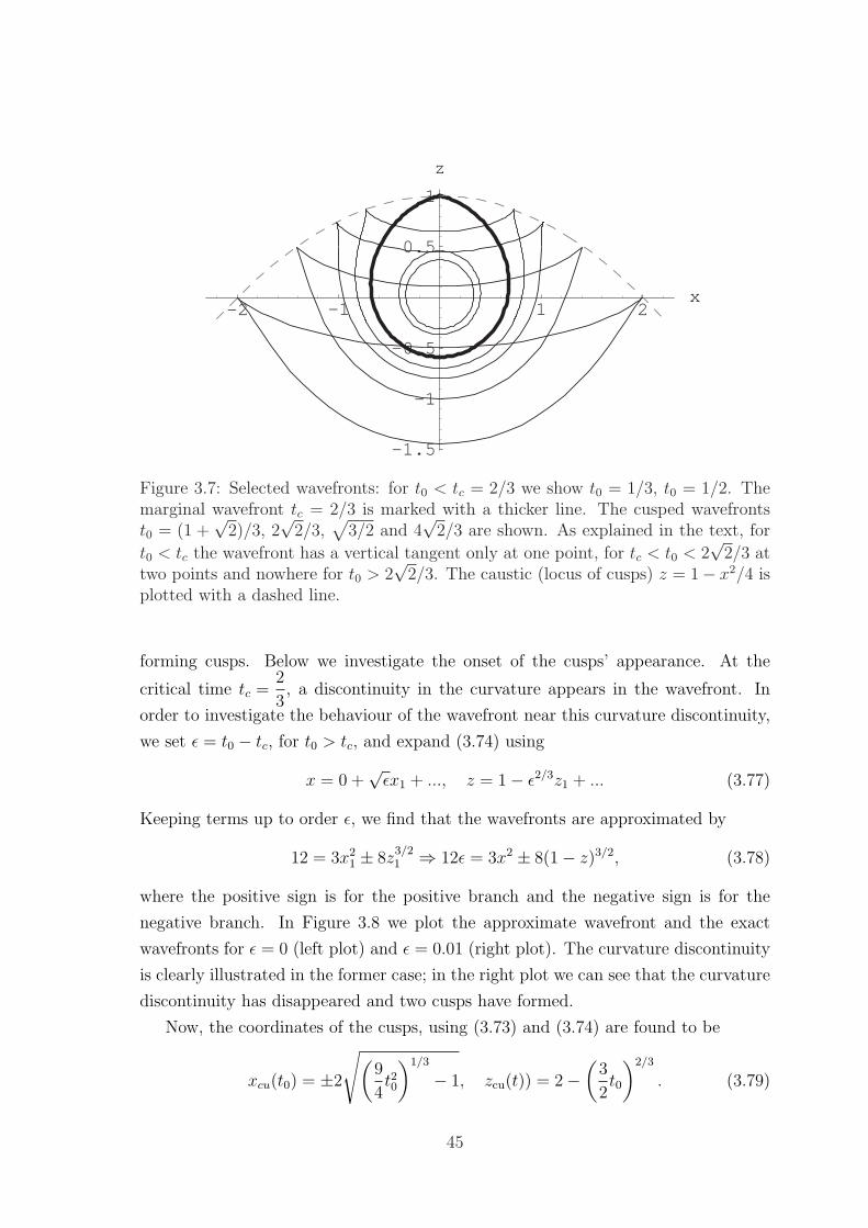
-2 -1 1 2x
-1.5
-1
-0.5
0.5
1
z
Figure 3.7: Selected wavefronts: for t0 < tc = 2/3 we show t0 = 1/3, t0 = 1/2. Themarginal wavefront tc = 2/3 is marked with a thicker line. The cusped wavefrontst0 = (1 +
√2)/3, 2
√2/3,
√3/2 and 4
√2/3 are shown. As explained in the text, for
t0 < tc the wavefront has a vertical tangent only at one point, for tc < t0 < 2√
2/3 attwo points and nowhere for t0 > 2
√2/3. The caustic (locus of cusps) z = 1− x2/4 is
plotted with a dashed line.
forming cusps. Below we investigate the onset of the cusps’ appearance. At the
critical time tc =2
3, a discontinuity in the curvature appears in the wavefront. In
order to investigate the behaviour of the wavefront near this curvature discontinuity,
we set ε = t0 − tc, for t0 > tc, and expand (3.74) using
x = 0 +√εx1 + ..., z = 1− ε2/3z1 + ... (3.77)
Keeping terms up to order ε, we find that the wavefronts are approximated by
12 = 3x21 ± 8z
3/21 ⇒ 12ε = 3x2 ± 8(1− z)3/2, (3.78)
where the positive sign is for the positive branch and the negative sign is for the
negative branch. In Figure 3.8 we plot the approximate wavefront and the exact
wavefronts for ε = 0 (left plot) and ε = 0.01 (right plot). The curvature discontinuity
is clearly illustrated in the former case; in the right plot we can see that the curvature
discontinuity has disappeared and two cusps have formed.
Now, the coordinates of the cusps, using (3.73) and (3.74) are found to be
xcu(t0) = ±2
√(9
4t20
)1/3
− 1, zcu(t)) = 2−(
3
2t0
)2/3
. (3.79)
45
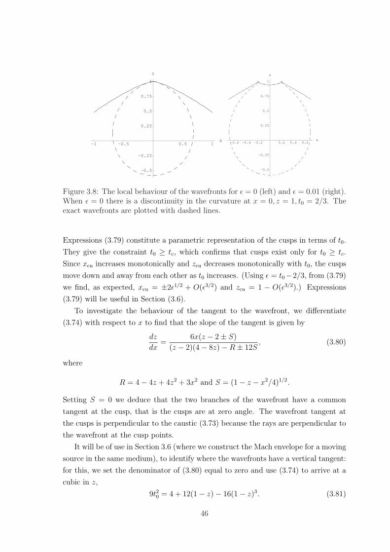
-1 -0.5 0.5 1x
-0.5
-0.25
0.25
0.5
0.75
1
z
-0.6 -0.4 -0.2 0.2 0.4 0.6x
-0.5
-0.25
0.25
0.5
0.75
1
z
Figure 3.8: The local behaviour of the wavefronts for ε = 0 (left) and ε = 0.01 (right).When ε = 0 there is a discontinuity in the curvature at x = 0, z = 1, t0 = 2/3. Theexact wavefronts are plotted with dashed lines.
Expressions (3.79) constitute a parametric representation of the cusps in terms of t0.
They give the constraint t0 ≥ tc, which confirms that cusps exist only for t0 ≥ tc.
Since xcu increases monotonically and zcu decreases monotonically with t0, the cusps
move down and away from each other as t0 increases. (Using ε = t0−2/3, from (3.79)
we find, as expected, xcu = ±2ε1/2 + O(ε3/2) and zcu = 1 − O(ε3/2).) Expressions
(3.79) will be useful in Section (3.6).
To investigate the behaviour of the tangent to the wavefront, we differentiate
(3.74) with respect to x to find that the slope of the tangent is given by
dz
dx=
6x(z − 2± S)
(z − 2)(4− 8z)−R± 12S, (3.80)
where
R = 4− 4z + 4z2 + 3x2 and S = (1− z − x2/4)1/2.
Setting S = 0 we deduce that the two branches of the wavefront have a common
tangent at the cusp, that is the cusps are at zero angle. The wavefront tangent at
the cusps is perpendicular to the caustic (3.73) because the rays are perpendicular to
the wavefront at the cusp points.
It will be of use in Section 3.6 (where we construct the Mach envelope for a moving
source in the same medium), to identify where the wavefronts have a vertical tangent:
for this, we set the denominator of (3.80) equal to zero and use (3.74) to arrive at a
cubic in z,
9t20 = 4 + 12(1− z)− 16(1− z)3. (3.81)
46
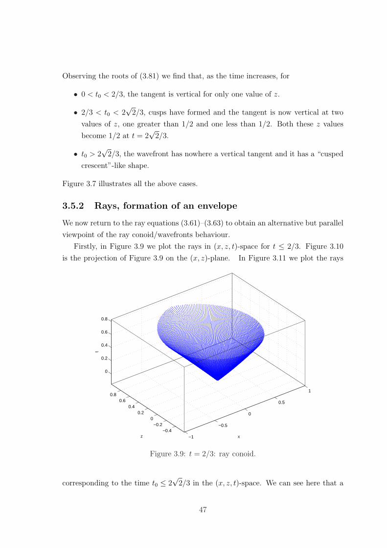
Observing the roots of (3.81) we find that, as the time increases, for
• 0 < t0 < 2/3, the tangent is vertical for only one value of z.
• 2/3 < t0 < 2√
2/3, cusps have formed and the tangent is now vertical at two
values of z, one greater than 1/2 and one less than 1/2. Both these z values
become 1/2 at t = 2√
2/3.
• t0 > 2√
2/3, the wavefront has nowhere a vertical tangent and it has a “cusped
crescent”-like shape.
Figure 3.7 illustrates all the above cases.
3.5.2 Rays, formation of an envelope
We now return to the ray equations (3.61)–(3.63) to obtain an alternative but parallel
viewpoint of the ray conoid/wavefronts behaviour.
Firstly, in Figure 3.9 we plot the rays in (x, z, t)-space for t ≤ 2/3. Figure 3.10
is the projection of Figure 3.9 on the (x, z)-plane. In Figure 3.11 we plot the rays
−1
−0.5
0
0.5
1
−0.4−0.2
00.2
0.40.6
0.8
0
0.2
0.4
0.6
0.8
xz
t
Figure 3.9: t = 2/3: ray conoid.
corresponding to the time t0 ≤ 2√
2/3 in the (x, z, t)-space. We can see here that a
47
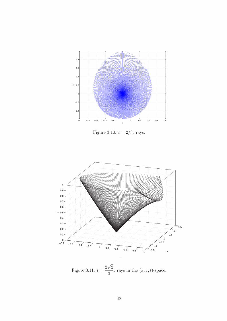
−1 −0.8 −0.6 −0.4 −0.2 0 0.2 0.4 0.6 0.8 1
−0.4
−0.2
0
0.2
0.4
0.6
0.8
x
z
Figure 3.10: t = 2/3: rays.
−0.8 −0.6 −0.4 −0.2 0 0.2 0.4 0.6 0.8 1−1.5
−1
−0.5
0
0.5
1
1.5
0
0.1
0.2
0.3
0.4
0.5
0.6
0.7
0.8
0.9
1
x
z
t
Figure 3.11: t =2√
2
3: rays in the (x, z, t)-space.
48
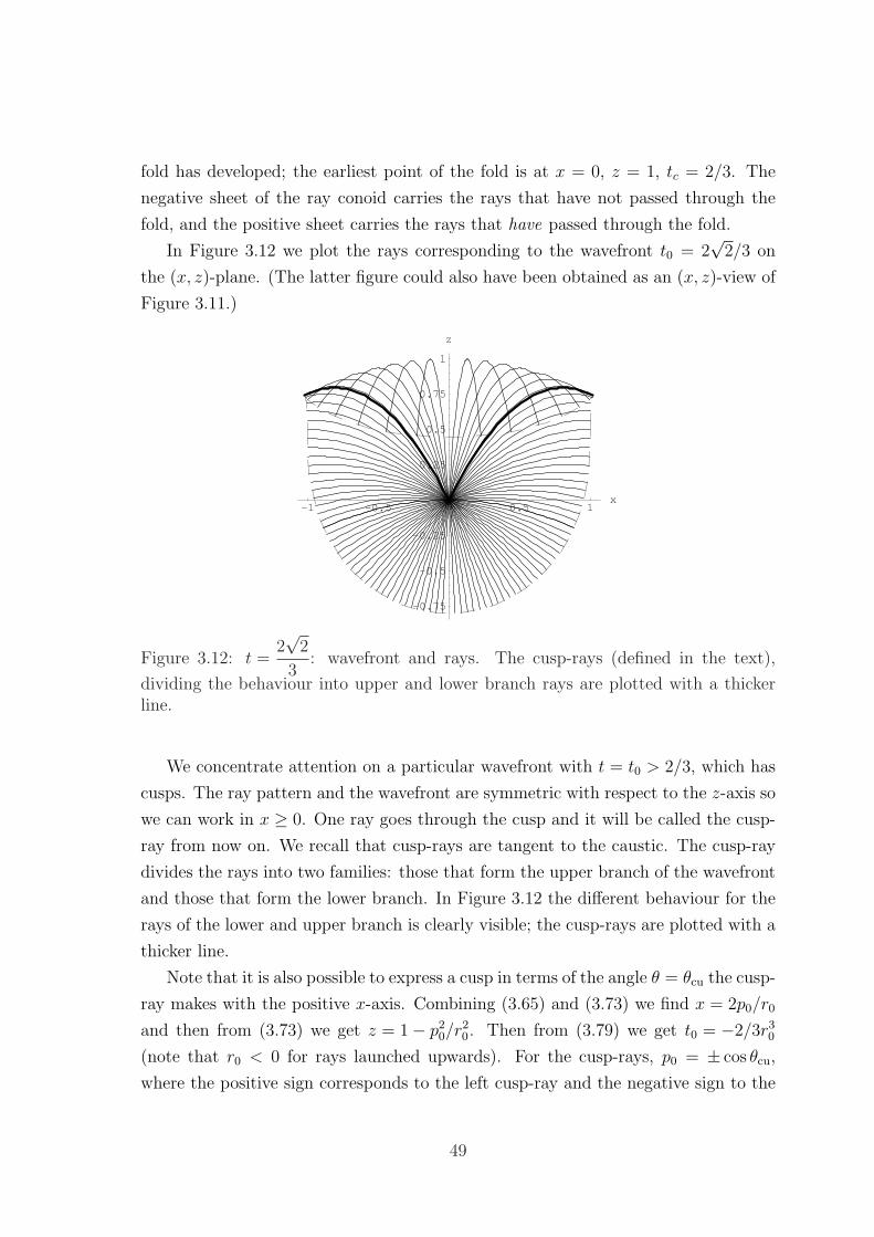
fold has developed; the earliest point of the fold is at x = 0, z = 1, tc = 2/3. The
negative sheet of the ray conoid carries the rays that have not passed through the
fold, and the positive sheet carries the rays that have passed through the fold.
In Figure 3.12 we plot the rays corresponding to the wavefront t0 = 2√
2/3 on
the (x, z)-plane. (The latter figure could also have been obtained as an (x, z)-view of
Figure 3.11.)
-1 -0.5 0.5 1x
-0.75
-0.5
-0.25
0.25
0.5
0.75
1
z
Figure 3.12: t =2√
2
3: wavefront and rays. The cusp-rays (defined in the text),
dividing the behaviour into upper and lower branch rays are plotted with a thickerline.
We concentrate attention on a particular wavefront with t = t0 > 2/3, which has
cusps. The ray pattern and the wavefront are symmetric with respect to the z-axis so
we can work in x ≥ 0. One ray goes through the cusp and it will be called the cusp-
ray from now on. We recall that cusp-rays are tangent to the caustic. The cusp-ray
divides the rays into two families: those that form the upper branch of the wavefront
and those that form the lower branch. In Figure 3.12 the different behaviour for the
rays of the lower and upper branch is clearly visible; the cusp-rays are plotted with a
thicker line.
Note that it is also possible to express a cusp in terms of the angle θ = θcu the cusp-
ray makes with the positive x-axis. Combining (3.65) and (3.73) we find x = 2p0/r0
and then from (3.73) we get z = 1− p20/r
20. Then from (3.79) we get t0 = −2/3r3
0
(note that r0 < 0 for rays launched upwards). For the cusp-rays, p0 = ± cos θcu,
where the positive sign corresponds to the left cusp-ray and the negative sign to the
49
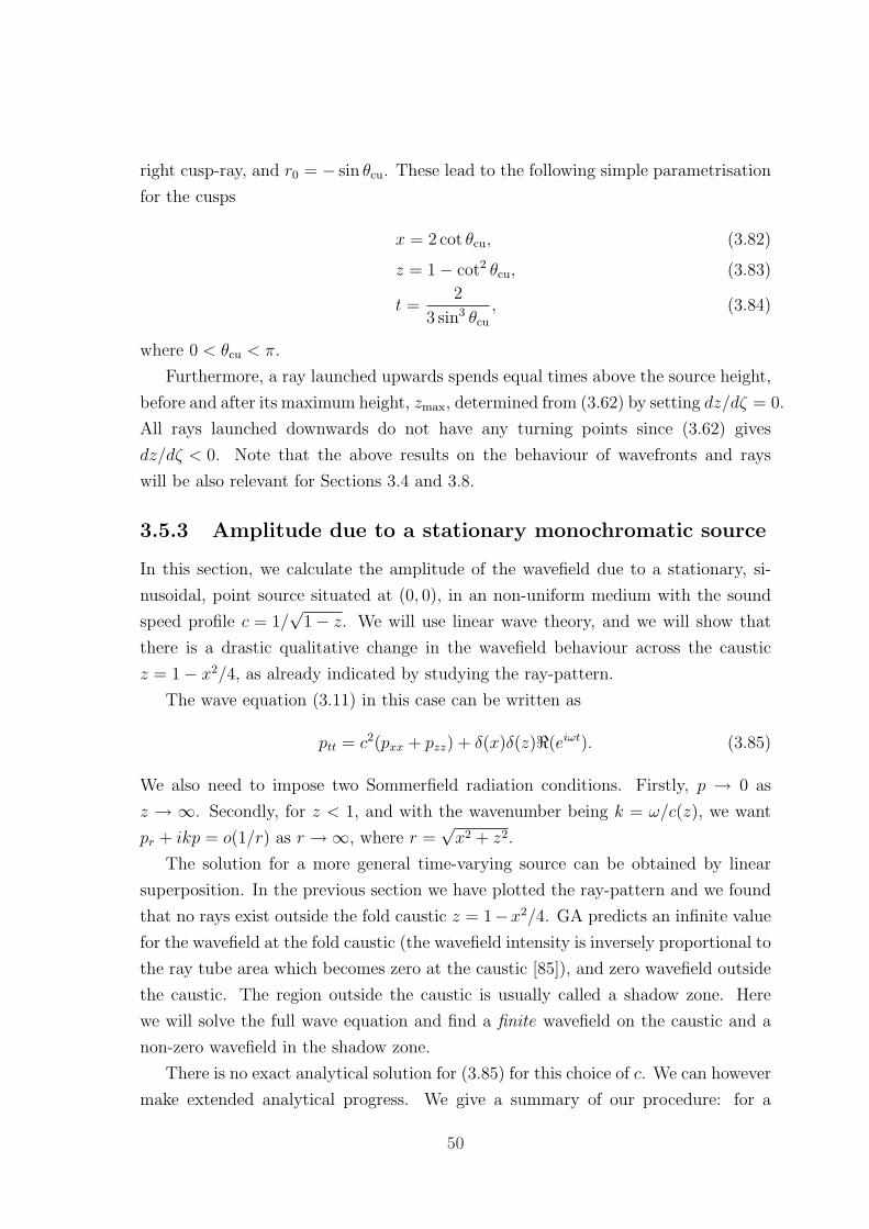
right cusp-ray, and r0 = − sin θcu. These lead to the following simple parametrisation
for the cusps
x = 2 cot θcu, (3.82)
z = 1− cot2 θcu, (3.83)
t =2
3 sin3 θcu
, (3.84)
where 0 < θcu < π.
Furthermore, a ray launched upwards spends equal times above the source height,
before and after its maximum height, zmax, determined from (3.62) by setting dz/dζ = 0.
All rays launched downwards do not have any turning points since (3.62) gives
dz/dζ < 0. Note that the above results on the behaviour of wavefronts and rays
will be also relevant for Sections 3.4 and 3.8.
3.5.3 Amplitude due to a stationary monochromatic source
In this section, we calculate the amplitude of the wavefield due to a stationary, si-
nusoidal, point source situated at (0, 0), in an non-uniform medium with the sound
speed profile c = 1/√
1− z. We will use linear wave theory, and we will show that
there is a drastic qualitative change in the wavefield behaviour across the caustic
z = 1− x2/4, as already indicated by studying the ray-pattern.
The wave equation (3.11) in this case can be written as
ptt = c2(pxx + pzz) + δ(x)δ(z)<(eiωt). (3.85)
We also need to impose two Sommerfield radiation conditions. Firstly, p → 0 as
z → ∞. Secondly, for z < 1, and with the wavenumber being k = ω/c(z), we want
pr + ikp = o(1/r) as r →∞, where r =√x2 + z2.
The solution for a more general time-varying source can be obtained by linear
superposition. In the previous section we have plotted the ray-pattern and we found
that no rays exist outside the fold caustic z = 1−x2/4. GA predicts an infinite value
for the wavefield at the fold caustic (the wavefield intensity is inversely proportional to
the ray tube area which becomes zero at the caustic [85]), and zero wavefield outside
the caustic. The region outside the caustic is usually called a shadow zone. Here
we will solve the full wave equation and find a finite wavefield on the caustic and a
non-zero wavefield in the shadow zone.
There is no exact analytical solution for (3.85) for this choice of c. We can however
make extended analytical progress. We give a summary of our procedure: for a
50
monochromatic disturbance equation (3.85) reduces to an inhomogeneous Helmholtz
equation, on which we perform a Fourier transform in the x-direction. This leads
to an inhomogeneous Airy equation (under a suitable transformation) which is then
solved analytically with appropriate boundary conditions on the behaviour of solution
at infinity and at the source height. The transform is then inverted numerically. This
procedure is valid for all values of ω.
Starting, we substitute
p(x, z, t) = <(exp(iωt)U(x, z)), (3.86)
in (3.85) and we obtain the inhomogeneous Helmholtz equation
−ω2U = c2(Uxx + Uzz) + δ(x)δ(z). (3.87)
We then take the Fourier Transform of (3.87) with respect to x, defining
U(α, z) =
∫ ∞
−∞U(x, z) exp (iαx)dx. (3.88)
We thus obtain
d2U
dz2+
(ω2
c2− α2
)U +
δ(z)
c2= 0. (3.89)
Note that equation (3.89) is valid for any choice of c; for the special case of c2 = 1/(1− z),
and letting z = ω2/3(z−1+α2/ω2) we obtain from it the inhomogeneous Airy equation
d2U
dz2= zU − ω−2/3δ(z − zs). (3.90)
(We note that for a linear speed profile equation (3.89) reduces to a Bessel equation
that admits solutions in terms of Bessel functions of imaginary arguments.) The
general solution of (3.90) is given by
U(α, z) =
{U1(α, z) = A1Ai(z) +B1Bi(z), z ≥ zsU2(α, z) = A2Ai(z) +B2Bi(z), z ≤ zs
where Ai(x) is the Airy function of the first kind and Bi(x) is the Airy function of
the second kind (see Figure 3.13) and zs is the value of z at the source height z = 0.
We have therefore four unknowns A1, B1, A2, B2 and to determine them, we need four
conditions. The first condition to impose is that U → 0 as z →∞. Since Bi(z) →∞in this limit, we have to set B1 = 0. The second condition is that U has to represent
an outgoing wave as z → −∞. This leads to the relation A2 + iB2 → 0 as z → −∞.
51
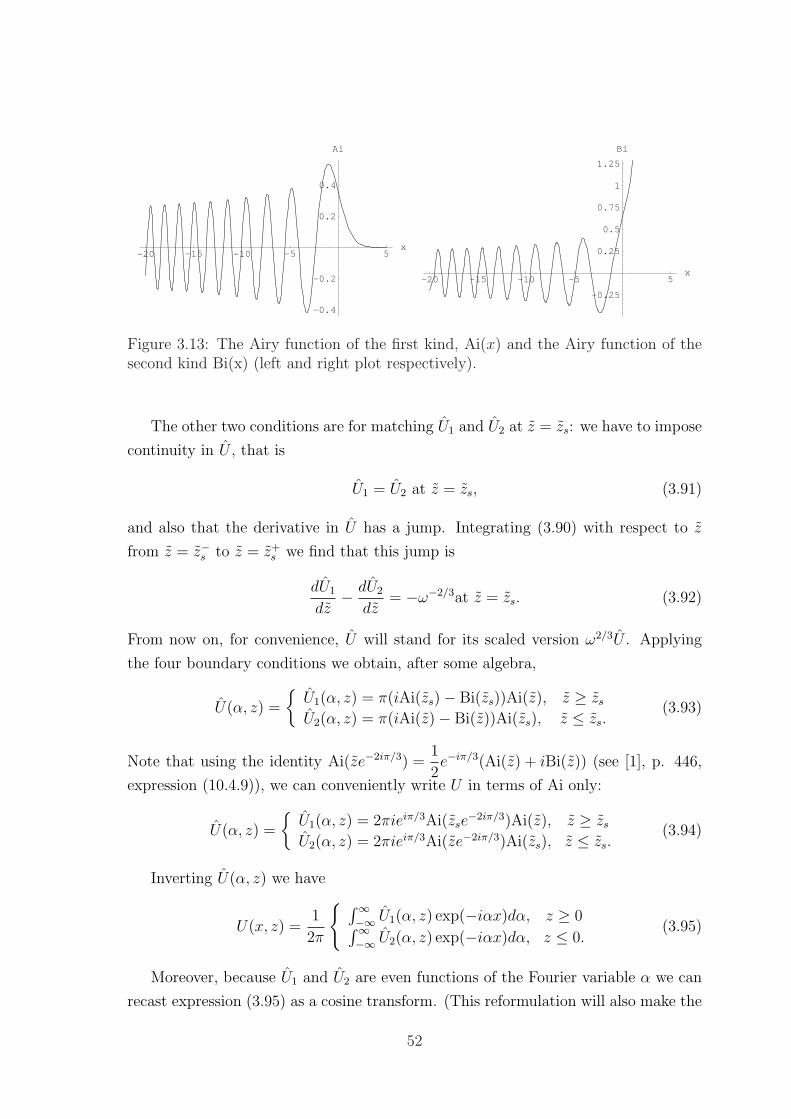
-20 -15 -10 -5 5x
-0.4
-0.2
0.2
0.4
Ai
-20 -15 -10 -5 5x
-0.25
0.25
0.5
0.75
1
1.25
Bi
Figure 3.13: The Airy function of the first kind, Ai(x) and the Airy function of thesecond kind Bi(x) (left and right plot respectively).
The other two conditions are for matching U1 and U2 at z = zs: we have to impose
continuity in U , that is
U1 = U2 at z = zs, (3.91)
and also that the derivative in U has a jump. Integrating (3.90) with respect to z
from z = z−s to z = z+s we find that this jump is
dU1
dz− dU2
dz= −ω−2/3at z = zs. (3.92)
From now on, for convenience, U will stand for its scaled version ω2/3U . Applying
the four boundary conditions we obtain, after some algebra,
U(α, z) =
{U1(α, z) = π(iAi(zs)− Bi(zs))Ai(z), z ≥ zsU2(α, z) = π(iAi(z)− Bi(z))Ai(zs), z ≤ zs.
(3.93)
Note that using the identity Ai(ze−2iπ/3) =1
2e−iπ/3(Ai(z) + iBi(z)) (see [1], p. 446,
expression (10.4.9)), we can conveniently write U in terms of Ai only:
U(α, z) =
{U1(α, z) = 2πieiπ/3Ai(zse
−2iπ/3)Ai(z), z ≥ zsU2(α, z) = 2πieiπ/3Ai(ze−2iπ/3)Ai(zs), z ≤ zs.
(3.94)
Inverting U(α, z) we have
U(x, z) =1
2π
{ ∫∞−∞ U1(α, z) exp(−iαx)dα, z ≥ 0∫∞−∞ U2(α, z) exp(−iαx)dα, z ≤ 0.
(3.95)
Moreover, because U1 and U2 are even functions of the Fourier variable α we can
recast expression (3.95) as a cosine transform. (This reformulation will also make the
52
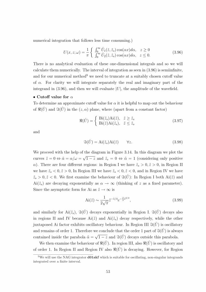
numerical integration that follows less time consuming.)
U(x, z;ω) =1
π
{ ∫∞0U1(z, zs) cos(αx)dα, z ≥ 0∫∞
0U2(z, zs) cos(αx)dα, z ≤ 0.
(3.96)
There is no analytical evaluation of these one-dimensional integrals and so we will
calculate them numerically. The interval of integration as seen in (3.96) is semiinfinite,
and for our numerical method9 we need to truncate at a suitably chosen cutoff value
of α. For clarity we will integrate separately the real and imaginary part of the
integrand in (3.96), and then we will evaluate |U |, the amplitude of the wavefield.
• Cutoff value for α
To determine an approximate cutoff value for α it is helpful to map out the behaviour
of <(U) and =(U) in the (z, α) plane, where (apart from a constant factor)
<(U) =
{Bi(zs)Ai(z), z ≥ zsBi(z)Ai(zs), z ≤ zs
(3.97)
and
=(U) = Ai(zs)Ai(z) ∀z. (3.98)
We proceed with the help of the diagram in Figure 3.14. In this diagram we plot the
curves z = 0 ⇔ α = α/ω =√
1− z and zs = 0 ⇔ α = 1 (considering only positive
α). There are four different regions: in Region I we have zs > 0, z > 0, in Region II
we have zs < 0, z > 0, In Region III we have zs < 0, z < 0, and in Region IV we have
zs > 0, z < 0. We first examine the behaviour of =(U): In Region I both Ai(z) and
Ai(zs) are decaying exponentially as α → ∞ (thinking of z as a fixed parameter).
Since the asymptotic form for Ai as z →∞ is
Ai(z) ∼ 1
2√πz−1/4e−
23z3/2
, (3.99)
and similarly for Ai(zs), =(U) decays exponentially in Region I. =(U) decays also
in regions II and IV because Ai(z) and Ai(zs) decay respectively, while the other
juxtaposed Ai factor exhibits oscillatory behaviour. In Region III =(U) is oscillatory
and remains of order 1. Therefore we conclude that the order 1 part of =(U) is always
contained inside the parabola α =√
1− z and =(U) decays outside this parabola.
We then examine the behaviour of <(U). In region III, also <(U) is oscillatory and
of order 1. In Region II and Region IV also <(U) is decaying. However, for Region
9We will use the NAG integrator d01akf which is suitable for oscillating, non-singular integrandsintegrated over a finite interval.
53
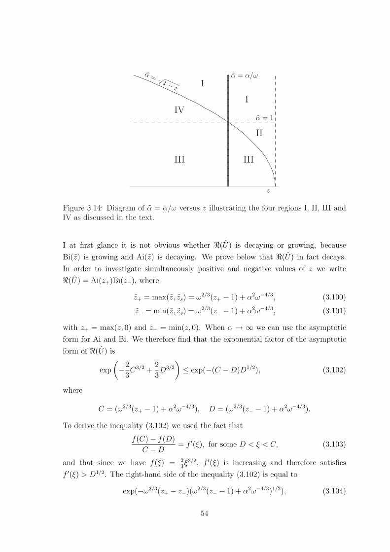
I
II
IIIIII
IV
Iα = √
1− z
α = α/ω
z
α = 1
Figure 3.14: Diagram of α = α/ω versus z illustrating the four regions I, II, III andIV as discussed in the text.
I at first glance it is not obvious whether <(U) is decaying or growing, because
Bi(z) is growing and Ai(z) is decaying. We prove below that <(U) in fact decays.
In order to investigate simultaneously positive and negative values of z we write
<(U) = Ai(z+)Bi(z−), where
z+ = max(z, zs) = ω2/3(z+ − 1) + α2ω−4/3, (3.100)
z− = min(z, zs) = ω2/3(z− − 1) + α2ω−4/3, (3.101)
with z+ = max(z, 0) and z− = min(z, 0). When α → ∞ we can use the asymptotic
form for Ai and Bi. We therefore find that the exponential factor of the asymptotic
form of <(U) is
exp
(−2
3C3/2 +
2
3D3/2
)≤ exp(−(C −D)D1/2), (3.102)
where
C = (ω2/3(z+ − 1) + α2ω−4/3), D = (ω2/3(z− − 1) + α2ω−4/3).
To derive the inequality (3.102) we used the fact that
f(C)− f(D)
C −D= f ′(ξ), for some D < ξ < C, (3.103)
and that since we have f(ξ) = 23ξ3/2, f ′(ξ) is increasing and therefore satisfies
f ′(ξ) > D1/2. The right-hand side of the inequality (3.102) is equal to
exp(−ω2/3(z+ − z−)(ω2/3(z− − 1) + α2ω−4/3)1/2), (3.104)
54
and this tends to zero as α→∞ when z+ > z−. Therefore we have proved that <(U)
decays in Region I, except when z = 0.
We therefore conclude that for a fixed z = z0 6= 0 and ω = ω0 a reasonable cutoff
value for α should be greater than ω0
√1− z0. In the numerical integration below we
will take the value of α appreciably larger than this estimated cutoff to ensure good
accuracy in |U |.• Plots of <U , =U and |U |.Below, we take the values ω = 10 and ω = 30 as representative cases of a moderate
and a high frequency, and we show plots of <(U), =(U) and |U |.¦ For ω = 10, taking the cutoff value to be α = 25, <(U), =(U) and |U | are plotted
in Figures 3.15–3.18.
Figure 3.15: <(U), ω = 10.
¦ For ω = 30, taking the cutoff value to be α = 50, <(U), =(U) and |U | are plotted
in Figures 3.19–3.22.
In the plots of <(U) and =(U) we see the wavelike nature of the wavefield inside
the caustic, and its decay in the shadow zone. In Figures 3.18 and 3.22 we see ridges,
more closely spaced in the latter than the former, which we explain below. The
behaviour of the wavefield for values of z > 1 is of interest, because c(z) goes to
infinity at z = 1 and therefore in Figures 3.18 and 3.22 we plot the wavefield up to
55
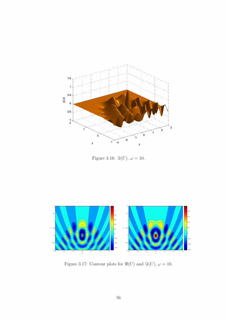
Figure 3.16: =(U), ω = 10.
x
z
−3 −2 −1 0 1 2 3−1
−0.5
0
0.5
1
1.5
2
−0.6
−0.4
−0.2
0
0.2
0.4
0.6
0.8
1
x
z
−3 −2 −1 0 1 2 3−1
−0.5
0
0.5
1
1.5
2
−0.6
−0.4
−0.2
0
0.2
0.4
0.6
0.8
Figure 3.17: Contour plots for <(U) and =(U), ω = 10.
56
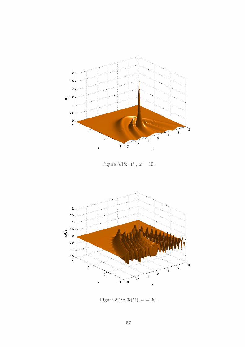
Figure 3.18: |U |, ω = 10.
Figure 3.19: <(U), ω = 30.
57
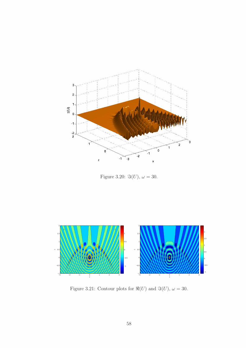
Figure 3.20: =(U), ω = 30.
x
z
−3 −2 −1 0 1 2 3−1
−0.5
0
0.5
1
1.5
2
−1
−0.5
0
0.5
1
x
z
−3 −2 −1 0 1 2 3−1
−0.5
0
0.5
1
1.5
2
−1
−0.5
0
0.5
1
1.5
2
Figure 3.21: Contour plots for <(U) and =(U), ω = 30.
58
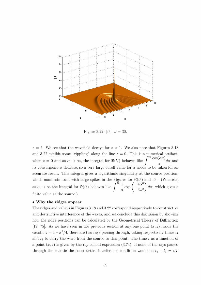
Figure 3.22: |U |, ω = 30.
z = 2. We see that the wavefield decays for z > 1. We also note that Figures 3.18
and 3.22 exhibit some “rippling” along the line z = 0. This is a numerical artifact;
when z = 0 and as α → ∞, the integral for <(U) behaves like
∫ ∞ cos(αx)
αdα and
its convergence is delicate, so a very large cutoff value for α needs to be taken for an
accurate result. This integral gives a logarithmic singularity at the source position,
which manifests itself with large spikes in the Figures for <(U) and |U |. (Whereas,
as α → ∞ the integral for =(U) behaves like
∫ ∞ 1
αexp
(−4α3
3ω2
)dα, which gives a
finite value at the source.)
• Why the ridges appear
The ridges and valleys in Figures 3.18 and 3.22 correspond respectively to constructive
and destructive interference of the waves, and we conclude this discussion by showing
how the ridge positions can be calculated by the Geometrical Theory of Diffraction
[19, 75]. As we have seen in the previous section at any one point (x, z) inside the
caustic z = 1− x2/4, there are two rays passing through, taking respectively times t1
and t2 to carry the wave from the source to this point. The time t as a function of
a point (x, z) is given by the ray conoid expression (3.74). If none of the rays passed
through the caustic the constructive interference condition would be t2 − t1 = nT
59
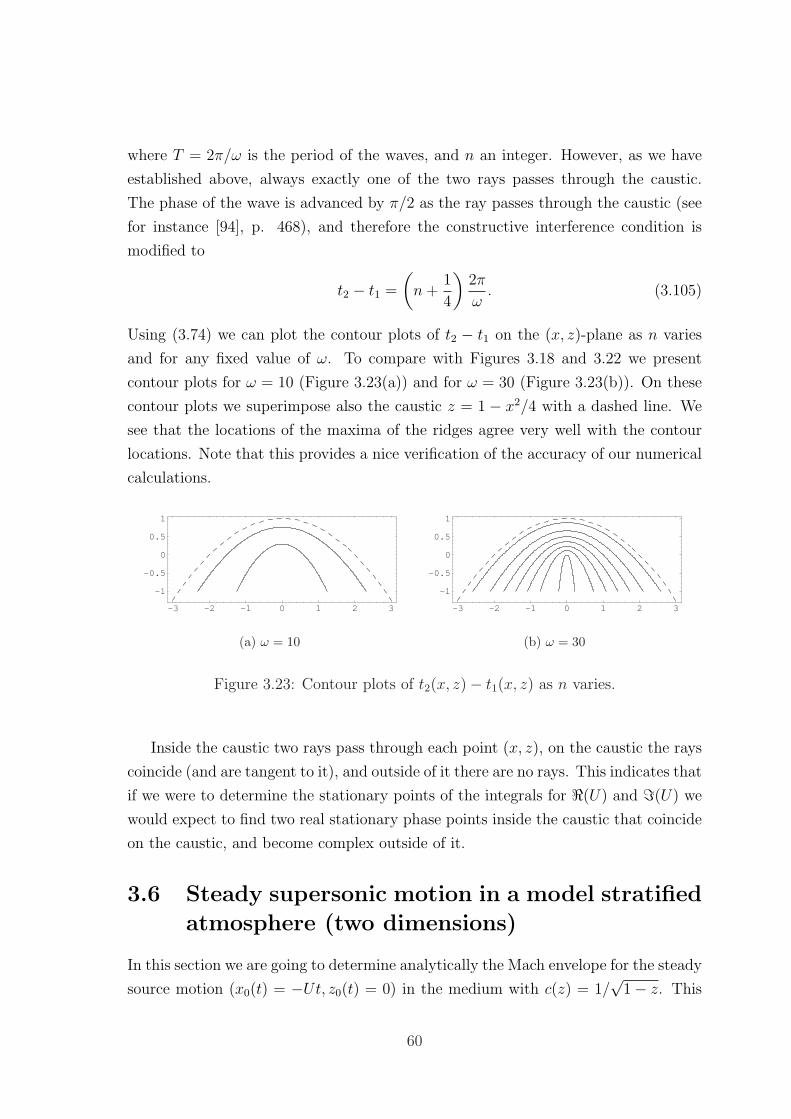
where T = 2π/ω is the period of the waves, and n an integer. However, as we have
established above, always exactly one of the two rays passes through the caustic.
The phase of the wave is advanced by π/2 as the ray passes through the caustic (see
for instance [94], p. 468), and therefore the constructive interference condition is
modified to
t2 − t1 =
(n+
1
4
)2π
ω. (3.105)
Using (3.74) we can plot the contour plots of t2 − t1 on the (x, z)-plane as n varies
and for any fixed value of ω. To compare with Figures 3.18 and 3.22 we present
contour plots for ω = 10 (Figure 3.23(a)) and for ω = 30 (Figure 3.23(b)). On these
contour plots we superimpose also the caustic z = 1 − x2/4 with a dashed line. We
see that the locations of the maxima of the ridges agree very well with the contour
locations. Note that this provides a nice verification of the accuracy of our numerical
calculations.
-3 -2 -1 0 1 2 3
-1
-0.5
0
0.5
1
(a) ω = 10
-3 -2 -1 0 1 2 3
-1
-0.5
0
0.5
1
(b) ω = 30
Figure 3.23: Contour plots of t2(x, z)− t1(x, z) as n varies.
Inside the caustic two rays pass through each point (x, z), on the caustic the rays
coincide (and are tangent to it), and outside of it there are no rays. This indicates that
if we were to determine the stationary points of the integrals for <(U) and =(U) we
would expect to find two real stationary phase points inside the caustic that coincide
on the caustic, and become complex outside of it.
3.6 Steady supersonic motion in a model stratified
atmosphere (two dimensions)
In this section we are going to determine analytically the Mach envelope for the steady
source motion (x0(t) = −Ut, z0(t) = 0) in the medium with c(z) = 1/√
1− z. This
60
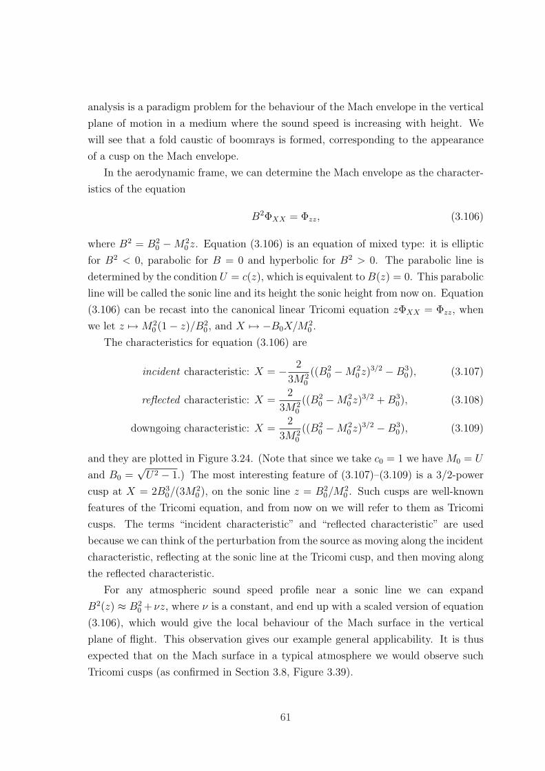
analysis is a paradigm problem for the behaviour of the Mach envelope in the vertical
plane of motion in a medium where the sound speed is increasing with height. We
will see that a fold caustic of boomrays is formed, corresponding to the appearance
of a cusp on the Mach envelope.
In the aerodynamic frame, we can determine the Mach envelope as the character-
istics of the equation
B2ΦXX = Φzz, (3.106)
where B2 = B20 −M2
0 z. Equation (3.106) is an equation of mixed type: it is elliptic
for B2 < 0, parabolic for B = 0 and hyperbolic for B2 > 0. The parabolic line is
determined by the condition U = c(z), which is equivalent toB(z) = 0. This parabolic
line will be called the sonic line and its height the sonic height from now on. Equation
(3.106) can be recast into the canonical linear Tricomi equation zΦXX = Φzz, when
we let z 7→M20 (1− z)/B2
0 , and X 7→ −B0X/M20 .
The characteristics for equation (3.106) are
incident characteristic: X = − 2
3M20
((B20 −M2
0 z)3/2 −B3
0), (3.107)
reflected characteristic: X =2
3M20
((B20 −M2
0 z)3/2 +B3
0), (3.108)
downgoing characteristic: X =2
3M20
((B20 −M2
0 z)3/2 −B3
0), (3.109)
and they are plotted in Figure 3.24. (Note that since we take c0 = 1 we have M0 = U
and B0 =√U2 − 1.) The most interesting feature of (3.107)–(3.109) is a 3/2-power
cusp at X = 2B30/(3M
20 ), on the sonic line z = B2
0/M20 . Such cusps are well-known
features of the Tricomi equation, and from now on we will refer to them as Tricomi
cusps. The terms “incident characteristic” and “reflected characteristic” are used
because we can think of the perturbation from the source as moving along the incident
characteristic, reflecting at the sonic line at the Tricomi cusp, and then moving along
the reflected characteristic.
For any atmospheric sound speed profile near a sonic line we can expand
B2(z) ≈ B20 + νz, where ν is a constant, and end up with a scaled version of equation
(3.106), which would give the local behaviour of the Mach surface in the vertical
plane of flight. This observation gives our example general applicability. It is thus
expected that on the Mach surface in a typical atmosphere we would observe such
Tricomi cusps (as confirmed in Section 3.8, Figure 3.39).
61
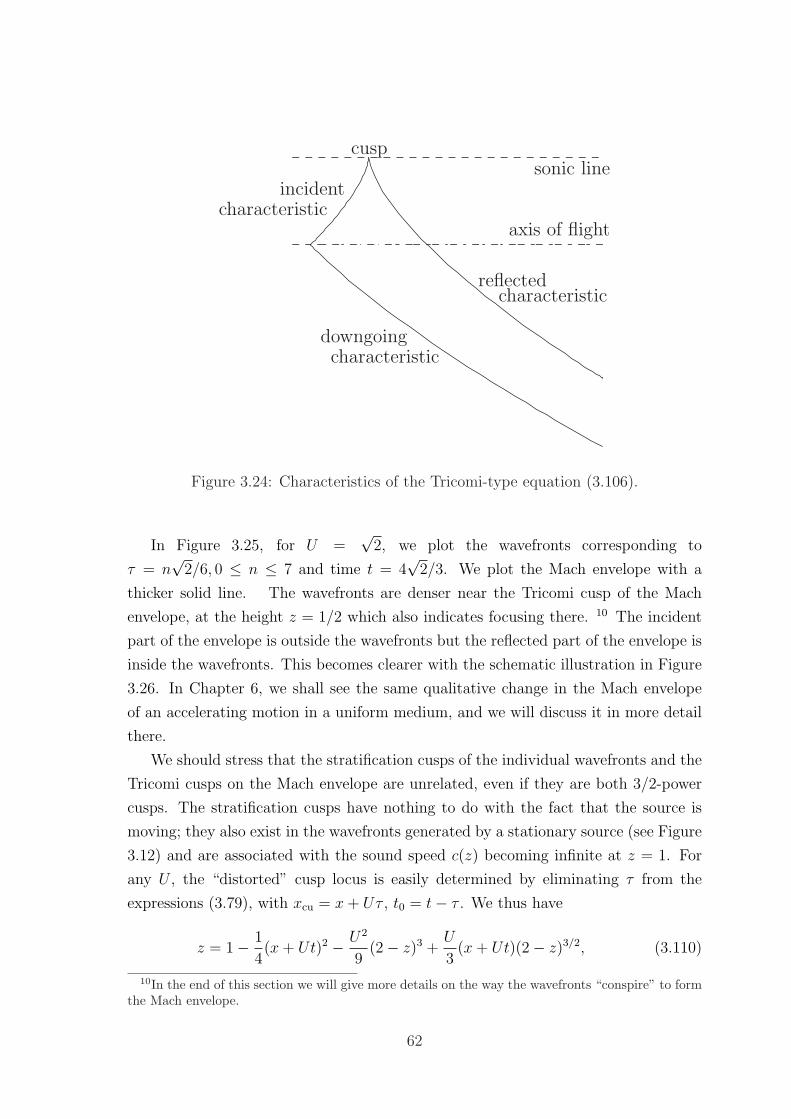
sonic line
axis of flight
cusp
reflectedcharacteristic
downgoingcharacteristic
incidentcharacteristic
Figure 3.24: Characteristics of the Tricomi-type equation (3.106).
In Figure 3.25, for U =√
2, we plot the wavefronts corresponding to
τ = n√
2/6, 0 ≤ n ≤ 7 and time t = 4√
2/3. We plot the Mach envelope with a
thicker solid line. The wavefronts are denser near the Tricomi cusp of the Mach
envelope, at the height z = 1/2 which also indicates focusing there. 10 The incident
part of the envelope is outside the wavefronts but the reflected part of the envelope is
inside the wavefronts. This becomes clearer with the schematic illustration in Figure
3.26. In Chapter 6, we shall see the same qualitative change in the Mach envelope
of an accelerating motion in a uniform medium, and we will discuss it in more detail
there.
We should stress that the stratification cusps of the individual wavefronts and the
Tricomi cusps on the Mach envelope are unrelated, even if they are both 3/2-power
cusps. The stratification cusps have nothing to do with the fact that the source is
moving; they also exist in the wavefronts generated by a stationary source (see Figure
3.12) and are associated with the sound speed c(z) becoming infinite at z = 1. For
any U , the “distorted” cusp locus is easily determined by eliminating τ from the
expressions (3.79), with xcu = x+ Uτ , t0 = t− τ . We thus have
z = 1− 1
4(x+ Ut)2 − U2
9(2− z)3 +
U
3(x+ Ut)(2− z)3/2, (3.110)
10In the end of this section we will give more details on the way the wavefronts “conspire” to formthe Mach envelope.
62
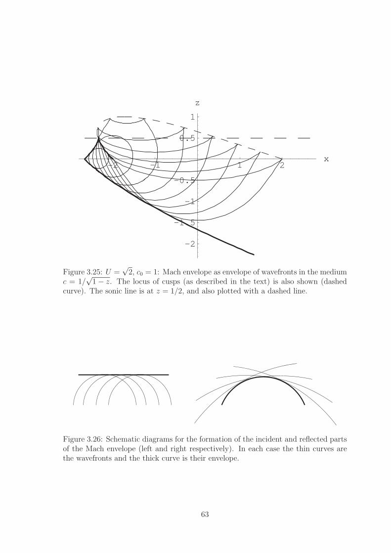
-2 -1 1 2x
-2
-1.5
-1
-0.5
0.5
1
z
Figure 3.25: U =√
2, c0 = 1: Mach envelope as envelope of wavefronts in the mediumc = 1/
√1− z. The locus of cusps (as described in the text) is also shown (dashed
curve). The sonic line is at z = 1/2, and also plotted with a dashed line.
Figure 3.26: Schematic diagrams for the formation of the incident and reflected partsof the Mach envelope (left and right respectively). In each case the thin curves arethe wavefronts and the thick curve is their envelope.
63
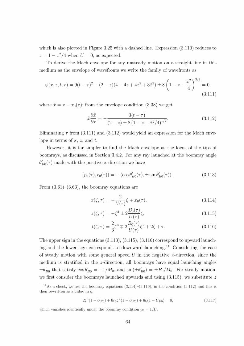
which is also plotted in Figure 3.25 with a dashed line. Expression (3.110) reduces to
z = 1− x2/4 when U = 0, as expected.
To derive the Mach envelope for any unsteady motion on a straight line in this
medium as the envelope of wavefronts we write the family of wavefronts as
ψ(x, z, t, τ) = 9(t− τ)2 − (2− z)(4− 4z + 4z2 + 3x2)± 8
(1− z − x2
4
)3/2
= 0,
(3.111)
where x = x− x0(τ); from the envelope condition (3.38) we get
x∂x
∂τ= − 3(t− τ)
(2− z)± 8 (1− z − x2/4)1/2. (3.112)
Eliminating τ from (3.111) and (3.112) would yield an expression for the Mach enve-
lope in terms of x, z, and t.
However, it is far simpler to find the Mach envelope as the locus of the tips of
boomrays, as discussed in Section 3.4.2. For any ray launched at the boomray angle
θ′B0(τ) made with the positive x-direction we have
(p0(τ), r0(τ)) = − (cos θ′B0(τ),± sin θ′B0(τ)) . (3.113)
From (3.61)–(3.63), the boomray equations are
x(ζ, τ) = − 2
U(τ)ζ + x0(τ), (3.114)
z(ζ, τ) = −ζ2 ± 2B0(τ)
U(τ)ζ, (3.115)
t(ζ, τ) =2
3ζ3 ∓ 2
B0(τ)
U(τ)ζ2 + 2ζ + τ. (3.116)
The upper sign in the equations (3.113), (3.115), (3.116) correspond to upward launch-
ing and the lower sign corresponds to downward launching.11 Considering the case
of steady motion with some general speed U in the negative x-direction, since the
medium is stratified in the z-direction, all boomrays have equal launching angles
±θ′B0 that satisfy cos θ′B0 = −1/M0, and sin(±θ′B0) = ±B0/M0. For steady motion,
we first consider the boomrays launched upwards and using (3.115), we substitute z
11As a check, we use the boomray equations (3.114)–(3.116), in the condition (3.112) and this isthen rewritten as a cubic in ζ,
2ζ3(1− Up0) + 6r0ζ2(1− Up0) + 6ζ(1− Up0) = 0, (3.117)
which vanishes identically under the boomray condition p0 = 1/U .
64
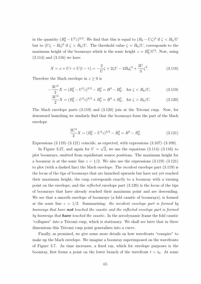
in the quantity (B20 − U2z)3/2. We find that this is equal to (B0 − Uζ)3 if ζ < B0/U
but to (Uζ − B0)3 if ζ > B0/U . The threshold value ζ = B0/U , corresponds to the
maximum height of the boomrays which is the sonic height z = B20/U
2. Now, using
(3.114) and (3.116) we have
X = x+ Uτ + U(t− τ) = − 2
Uζ + 2ζU − 2B0ζ
2 +2U
3ζ3. (3.118)
Therefore the Mach envelope in z ≥ 0 is
−3U2
2X = (B2
0 − U2z)3/2 −B30 = B3 −B3
0 , for ζ < B0/U, (3.119)
3U2
2X = (B2
0 − U2z)3/2 +B30 = B3 +B3
0 , for ζ > B0/U. (3.120)
The Mach envelope parts (3.119) and (3.120) join at the Tricomi cusp. Now, for
downward launching we similarly find that the boomrays form the part of the Mach
envelope
3U2
2X = (B2
0 − U2z)3/2 −B30 = B3 −B3
0 . (3.121)
Expressions (3.119)–(3.121) coincide, as expected, with expressions (3.107)–(3.109).
In Figure 3.27, and again for U =√
2, we use the equations (3.114)–(3.116) to
plot boomrays, emitted from equidistant source positions. The maximum height for
a boomray is at the sonic line z = 1/2. We also use the expressions (3.119)–(3.121)
to plot (with a dashed line) the Mach envelope. The incident envelope part (3.119) is
the locus of the tips of boomrays that are launched upwards but have not yet reached
their maximum height; the cusp corresponds exactly to a boomray with a turning
point on the envelope; and the reflected envelope part (3.120) is the locus of the tips
of boomrays that have already reached their maximum point and are descending.
We see that a smooth envelope of boomrays (a fold caustic of boomrays), is formed
at the sonic line z = 1/2. Summarising: the incident envelope part is formed by
boomrays that have not touched the caustic and the reflected envelope part is formed
by boomrays that have touched the caustic. In the aerodynamic frame the fold caustic
“collapses” into a Tricomi cusp, which is stationary. We shall see later that in three
dimensions this Tricomi cusp point generalises into a curve.
Finally, as promised, we give some more details on how wavefronts “conspire” to
make up the Mach envelope. We imagine a boomray superimposed on the wavefronts
of Figure 3.7. As time increases, a fixed ray, which for envelope purposes is the
boomray, first forms a point on the lower branch of the wavefront t = t0. At some
65
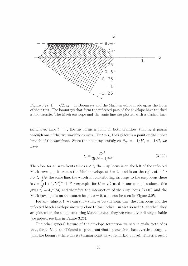
-2 -1 1x
-1.25
-1
-0.75
-0.5
-0.25
0.25
0.5
z
Figure 3.27: U =√
2, c0 = 1: Boomrays and the Mach envelope made up as the locusof their tips. The boomrays that form the reflected part of the envelope have toucheda fold caustic. The Mach envelope and the sonic line are plotted with a dashed line.
switchover time t = t? the ray forms a point on both branches, that is, it passes
through one of the two wavefront cusps. For t > t? the ray forms a point on the upper
branch of the wavefront. Since the boomrays satisfy cos θ′B0 = −1/M0 = −1/U , we
have
t? =2U3
3(U2 − 1)3/2. (3.122)
Therefore for all wavefronts times t < t? the cusp locus is on the left of the reflected
Mach envelope, it crosses the Mach envelope at t = t?, and is on the right of it for
t > t?. (At the sonic line, the wavefront contributing its cusps to the cusp locus there
is t =2
3(1 + 1/U2)3/2.) For example, for U =
√2 used in our examples above, this
gives t? = 4√
2/3) and therefore the intersection of the cusp locus (3.110) and the
Mach envelope is on the source height z = 0, as it can be seen in Figure 3.25.
For any value of U we can show that, below the sonic line, the cusp locus and the
reflected Mach envelope are very close to each other—in fact so near that when they
are plotted on the computer (using Mathematica) they are virtually indistinguishable
(we indeed see this in Figure 3.25).
The other general feature of the envelope formation we should make note of is
that, for all U , at the Tricomi cusp the contributing wavefront has a vertical tangent,
(and the boomray there has its turning point as we remarked above). This is a result
66
valid for the local behaviour near the sonic line in any steady motion in any stratified
medium. From Section 3.5.1, for any U , the vertical-tangent wavefront is given by
tvt(U) =2√U2 − 1(U2 + 2)
3U3, (3.123)
and we can use the results in page 47 to determine, for any value of U , which vertical
tangency is the one contributing to the Tricomi cusp.
3.7 Steady subsonic motion in a model stratified
atmosphere (two dimensions)
It is also of interest to show the wavefront pattern in the medium c = 1/√
1− z when
the source motion is subsonic. In this case no boomrays are emitted and hence no
Mach envelope is formed. However we expect some interesting features to arise due to
the medium stratification. In Figure 3.28 we plot 12 wavefronts for M0 = 1/2, t = 2,
and τ = n/6, n = 0, ..., 11. The wavefronts that satisfy t − τ ≤ 2/3 are nested.
Looking only at wavefronts of the latter type, Figure 3.28 is qualitatively similar to
Figure 3.3 for steady subsonic motion. However the wavefronts with t − τ ≥ 2/3
are not nested due to the presence of the stratification cusps. A cusp locus forms as
in Figure 3.7, given again by the analytical expression (3.110) and we plot it with a
dashed line. Note that the sonic line is z = 1 − 1/U2 = −3, and also shown with a
dashed line. (The thicker line in Figure 3.28 represents the path of the source.)
3.8 Steady supersonic motion in two model strat-
ified atmospheres (three dimensions)
3.8.1 Introduction and overview
For the stratified medium with sound speed profile c = c0/√
1− µz, we have analysed
the geometry of the Mach envelope in two dimensions, and presented relevant plots
for the case c0 = 1, µ = 1, at constant speed U =√
2. We are now going to present
analytical examples in three dimensions. We will assume a steady motion and work
in the aerodynamic frame.
Of great practical interest is the intersection of the Mach surface with the ground,
called the carpet. A primary carpet (PC) is formed by BICHs launched downwards
and a secondary carpet (SC) is formed by BICHs launched upwards, which eventually
67
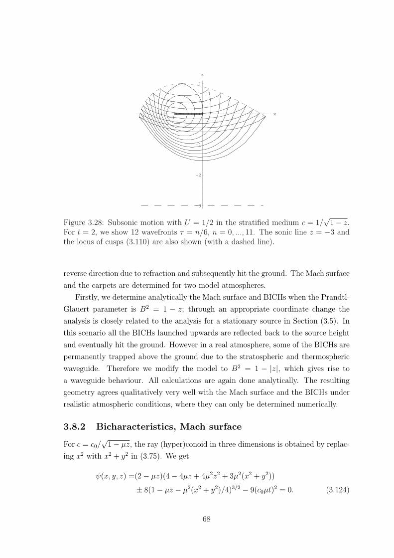
-2 -1 1 2x
-3
-2
-1
1
z
Figure 3.28: Subsonic motion with U = 1/2 in the stratified medium c = 1/√
1− z.For t = 2, we show 12 wavefronts τ = n/6, n = 0, ..., 11. The sonic line z = −3 andthe locus of cusps (3.110) are also shown (with a dashed line).
reverse direction due to refraction and subsequently hit the ground. The Mach surface
and the carpets are determined for two model atmospheres.
Firstly, we determine analytically the Mach surface and BICHs when the Prandtl-
Glauert parameter is B2 = 1 − z; through an appropriate coordinate change the
analysis is closely related to the analysis for a stationary source in Section (3.5). In
this scenario all the BICHs launched upwards are reflected back to the source height
and eventually hit the ground. However in a real atmosphere, some of the BICHs are
permanently trapped above the ground due to the stratospheric and thermospheric
waveguide. Therefore we modify the model to B2 = 1 − |z|, which gives rise to
a waveguide behaviour. All calculations are again done analytically. The resulting
geometry agrees qualitatively very well with the Mach surface and the BICHs under
realistic atmospheric conditions, where they can only be determined numerically.
3.8.2 Bicharacteristics, Mach surface
For c = c0/√
1− µz, the ray (hyper)conoid in three dimensions is obtained by replac-
ing x2 with x2 + y2 in (3.75). We get
ψ(x, y, z) =(2− µz)(4− 4µz + 4µ2z2 + 3µ2(x2 + y2))
± 8(1− µz − µ2(x2 + y2)/4)3/2 − 9(c0µt)2 = 0. (3.124)
68
One way to obtain the Mach surface for B2 = 1− z would be to take the envelope of
the ray conoids (3.124) with c0 = 1, µ = 1/2 and U =√
2 (or fix M0 = U/c0 =√
2 at
the reference level z0 = 0). However, this (lengthy) calculation can be circumvented
since for steady flight we can work with BICHs. The BICHs simplify the calculations
enormously as well as being the curves on which the boom propagates. Furthermore,
we will show that a change of coordinates in the ray conoid expression (3.74) will
give immediately the Mach surface here. When B2 = 1− z, the ordinary differential
equations for the BICHs cannot be analytically integrated if they are in the form
(3.54)–(3.55). We can resolve this if we work instead with the eikonal
F ′1 =1
2F1 =
1
2
(B2P − Q2 +R2
P
)= 0, (3.125)
which corresponds to the ordinary differential equations
dX
ds= MN + (M2, 0, 0), (3.126)
dN
ds= M
(−∇ c
c+ (N.
∇ c
c)N
), (3.127)
obtained directly from (3.54)–(3.55) by setting cdt = Mds. Integrating them we
obtain the BICHs equations
X(s;N0) =s3
12+R0
P0
s2
2+ (1− z0)s, (3.128)
y(s;N0) = −Q0
P0
s+ y0, (3.129)
z(s;N0) = −s2
4− R0
P0
s+ z0, (3.130)
P = P0, Q = Q0, r(s;N0) =P0
2s+R0, (3.131)
where
N0 =
(− 1
M0
,− Q0
M0P0
,− R0
M0P0
), (3.132)
is the unit outward normal to the Mach surface (see (3.56)) at the source location.
It is convenient to employ a spherical polar parametrisation where the azimuthal
angle ϕ is measured in the (y, z)-plane from the y-axis anticlockwise and θ is the
angle made with the positive x-direction. We therefore let
P0 = cos θ0 = − 1
M0
= constant, (3.133)
69
and then
Q0 = sin θ0 cosϕ =B0
M0
cosϕ, and R0 = sin θ0 sinϕ =B0
M0
sinϕ. (3.134)
Substituting (3.133) and (3.134) into the BICH equations (3.128)–(3.131) we have
X(s;ϕ) =s3
12− (B0 sinϕ)
s2
2+ (1− z0)s, (3.135)
y(s;ϕ) = −(B0 cosϕ)s+ y0, (3.136)
z(s;ϕ) = −s2
4+ (B0 sinϕ)s+ z0, (3.137)
r(s;ϕ) = − s
2M0
+1
M0
(B0 sinϕ), (3.138)
where B0 = B(z0) =√
1− z0. For BICHs launched upwards 0 ≤ ϕ ≤ π so sinϕ > 0,
and for BICHs launched downwards π ≤ ϕ ≤ 2π so sinϕ < 0.
To obtain the Mach surface we need to eliminate s and ϕ from (3.135)–(3.138).
However, this is unnecessary if we apply the coordinate transformation
t 7→ X, x 7→ y, z 7→ z (and p 7→ Φ), (3.139)
in equation (3.59), which then becomes equation (3.49). The ray conoid at (0, 0, 0)
of (3.59) is (3.74) and under the latter change of coordinates it leads immediately to
the required Mach surface for y0 = z0 = 0
9X2 = (2− z)(4− 4z + 4z2 + 3y2)± 8
(1− z − y2
4
)3/2
. (3.140)
Note that this is the same change of coordinates with which the theory of unsteady
cylindrical waves provides a shortcut in the analysis of the steady motion of an ax-
isymmetric body—see, for instance, Whitham [126], Section 7.5, p. 224. (Should we
wish to determine the Mach surface or any other expression for the more general case
of B2 = a− bz we can use in (3.140) (X, y, z) 7→ (a3/2X/b, ay/b, az/b).)
Obviously, the change of coordinates (3.139) makes the discussion of the features
of the ray conoid (3.74) for the stationary source directly relevant to the analysis
of the features of the Mach conoid (3.140) (and the discussion on the ray pattern
there directly relevant to the BICHs here). Firstly, Figure 3.7 no longer represents
wavefronts but instead (when we change the horizontal axis label to y) gives the
constant X-sections of the Mach conoid as X = X0 increases.
70
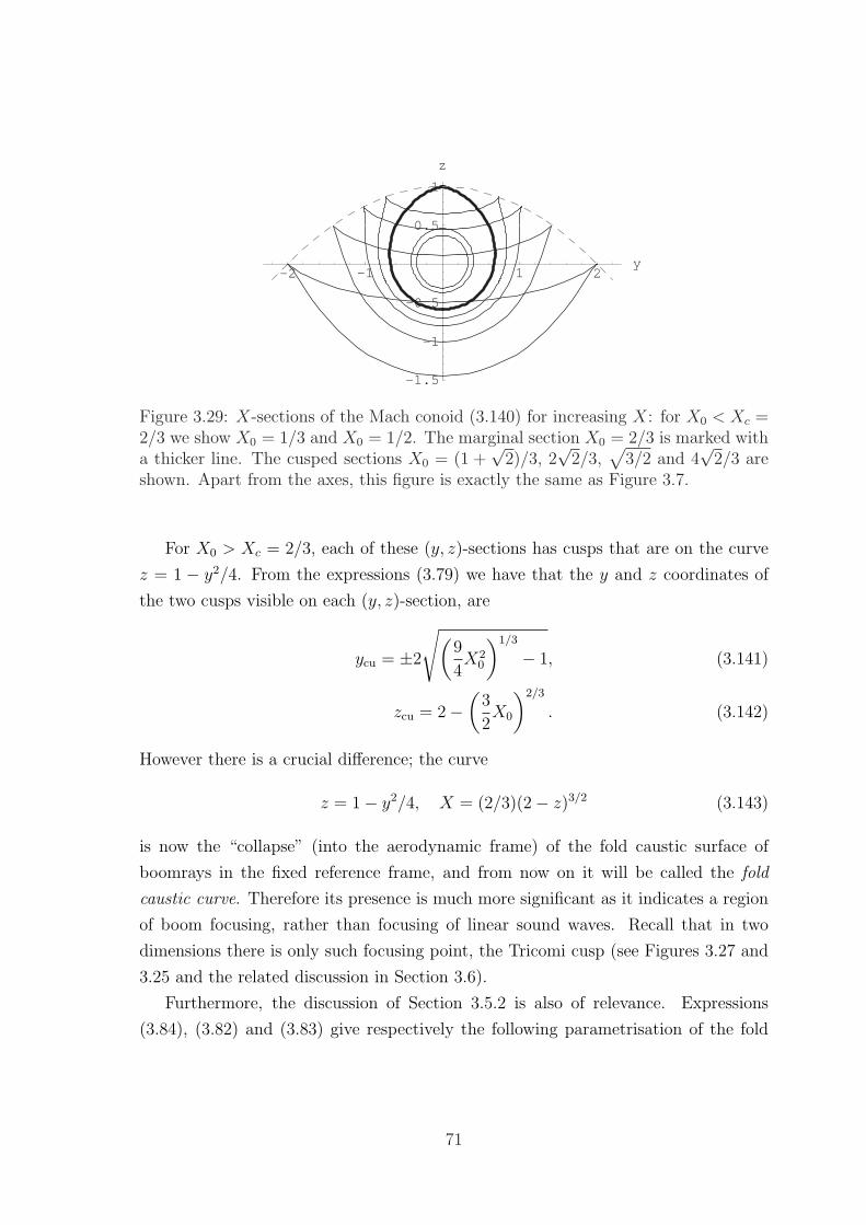
-2 -1 1 2y
-1.5
-1
-0.5
0.5
1
z
Figure 3.29: X-sections of the Mach conoid (3.140) for increasing X: for X0 < Xc =2/3 we show X0 = 1/3 and X0 = 1/2. The marginal section X0 = 2/3 is marked witha thicker line. The cusped sections X0 = (1 +
√2)/3, 2
√2/3,
√3/2 and 4
√2/3 are
shown. Apart from the axes, this figure is exactly the same as Figure 3.7.
For X0 > Xc = 2/3, each of these (y, z)-sections has cusps that are on the curve
z = 1 − y2/4. From the expressions (3.79) we have that the y and z coordinates of
the two cusps visible on each (y, z)-section, are
ycu = ±2
√(9
4X2
0
)1/3
− 1, (3.141)
zcu = 2−(
3
2X0
)2/3
. (3.142)
However there is a crucial difference; the curve
z = 1− y2/4, X = (2/3)(2− z)3/2 (3.143)
is now the “collapse” (into the aerodynamic frame) of the fold caustic surface of
boomrays in the fixed reference frame, and from now on it will be called the fold
caustic curve. Therefore its presence is much more significant as it indicates a region
of boom focusing, rather than focusing of linear sound waves. Recall that in two
dimensions there is only such focusing point, the Tricomi cusp (see Figures 3.27 and
3.25 and the related discussion in Section 3.6).
Furthermore, the discussion of Section 3.5.2 is also of relevance. Expressions
(3.84), (3.82) and (3.83) give respectively the following parametrisation of the fold
71
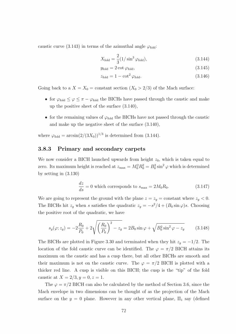
caustic curve (3.143) in terms of the azimuthal angle ϕfold:
Xfold =2
3(1/ sin3 ϕfold), (3.144)
yfold = 2 cotϕfold, (3.145)
zfold = 1− cot2 ϕfold. (3.146)
Going back to a X = X0 = constant section (X0 > 2/3) of the Mach surface:
• for ϕfold ≤ ϕ ≤ π − ϕfold the BICHs have passed through the caustic and make
up the positive sheet of the surface (3.140),
• for the remaining values of ϕfold the BICHs have not passed through the caustic
and make up the negative sheet of the surface (3.140),
where ϕfold = arcsin(2/(3X0))1/3 is determined from (3.144).
3.8.3 Primary and secondary carpets
We now consider a BICH launched upwards from height z0, which is taken equal to
zero. Its maximum height is reached at zmax = M20R
20 = B2
0 sin2 ϕ which is determined
by setting in (3.130)
dz
ds= 0 which corresponds to smax = 2M0R0. (3.147)
We are going to represent the ground with the plane z = zg = constant where zg < 0.
The BICHs hit zg when s satisfies the quadratic zg = −s2/4 + (B0 sinϕ)s. Choosing
the positive root of the quadratic, we have
sg(ϕ; zg) = −2R0
P0
+ 2
√(R0
P0
)2
− zg = 2B0 sinϕ+√B2
0 sin2 ϕ− zg (3.148)
The BICHs are plotted in Figure 3.30 and terminated when they hit zg = −1/2. The
location of the fold caustic curve can be identified. The ϕ = π/2 BICH attains its
maximum on the caustic and has a cusp there, but all other BICHs are smooth and
their maximum is not on the caustic curve. The ϕ = π/2 BICH is plotted with a
thicker red line. A cusp is visible on this BICH; the cusp is the “tip” of the fold
caustic at X = 2/3, y = 0, z = 1.
The ϕ = π/2 BICH can also be calculated by the method of Section 3.6, since the
Mach envelope in two dimensions can be thought of as the projection of the Mach
surface on the y = 0 plane. However in any other vertical plane, Π1 say (defined
72
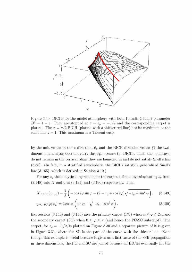
01
2X
-2
0
2y
-0.5
0
0.5
1
z
01
2X
-2
0
2y
Figure 3.30: BICHs for the model atmosphere with local Prandtl-Glauert parameterB2 = 1 − z. They are stopped at z = zg = −1/2 and the corresponding carpet isplotted. The ϕ = π/2 BICH (plotted with a thicker red line) has its maximum at thesonic line z = 1. This maximum is a Tricomi cusp.
by the unit vector in the z direction, ez and the BICH direction vector ξ) the two-
dimensional analysis does not carry through because the BICHs, unlike the boomrays,
do not remain in the vertical plane they are launched in and do not satisfy Snell’s law
(3.35). (In fact, in a stratified atmosphere, the BICHs satisfy a generalised Snell’s
law (3.165), which is derived in Section 3.10.)
For any zg the analytical expression for the carpet is found by substituting sg from
(3.148) into X and y in (3.135) and (3.136) respectively. Then
XPC–SC(ϕ; zg) =2
3
(− cos 2ϕ sinϕ− (2− zg + cos 2ϕ)
√−zg + sin2 ϕ
), (3.149)
yPC–SC(ϕ; zg) = 2 cosϕ
(sinϕ+
√−zg + sin2 ϕ
). (3.150)
Expressions (3.149) and (3.150) give the primary carpet (PC) when π ≤ ϕ ≤ 2π, and
the secondary carpet (SC) when 0 ≤ ϕ ≤ π (and hence the PC-SC subscript). The
carpet, for zg = −1/2, is plotted on Figure 3.30 and a separate picture of it is given
in Figure 3.31, where the SC is the part of the curve with the thicker line. Even
though this example is useful because it gives us a first taste of the SSB propagation
in three dimensions, the PC and SC are joined because all BICHs eventually hit the
73
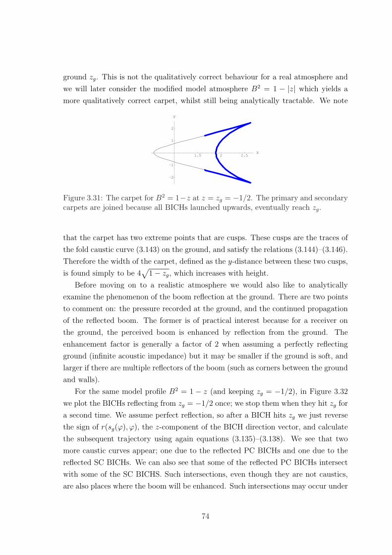
ground zg. This is not the qualitatively correct behaviour for a real atmosphere and
we will later consider the modified model atmosphere B2 = 1 − |z| which yields a
more qualitatively correct carpet, whilst still being analytically tractable. We note
1.5 2 2.5X
-2
-1
1
2
y
Figure 3.31: The carpet for B2 = 1−z at z = zg = −1/2. The primary and secondarycarpets are joined because all BICHs launched upwards, eventually reach zg.
that the carpet has two extreme points that are cusps. These cusps are the traces of
the fold caustic curve (3.143) on the ground, and satisfy the relations (3.144)–(3.146).
Therefore the width of the carpet, defined as the y-distance between these two cusps,
is found simply to be 4√
1− zg, which increases with height.
Before moving on to a realistic atmosphere we would also like to analytically
examine the phenomenon of the boom reflection at the ground. There are two points
to comment on: the pressure recorded at the ground, and the continued propagation
of the reflected boom. The former is of practical interest because for a receiver on
the ground, the perceived boom is enhanced by reflection from the ground. The
enhancement factor is generally a factor of 2 when assuming a perfectly reflecting
ground (infinite acoustic impedance) but it may be smaller if the ground is soft, and
larger if there are multiple reflectors of the boom (such as corners between the ground
and walls).
For the same model profile B2 = 1 − z (and keeping zg = −1/2), in Figure 3.32
we plot the BICHs reflecting from zg = −1/2 once; we stop them when they hit zg for
a second time. We assume perfect reflection, so after a BICH hits zg we just reverse
the sign of r(sg(ϕ), ϕ), the z-component of the BICH direction vector, and calculate
the subsequent trajectory using again equations (3.135)–(3.138). We see that two
more caustic curves appear; one due to the reflected PC BICHs and one due to the
reflected SC BICHs. We can also see that some of the reflected PC BICHs intersect
with some of the SC BICHS. Such intersections, even though they are not caustics,
are also places where the boom will be enhanced. Such intersections may occur under
74
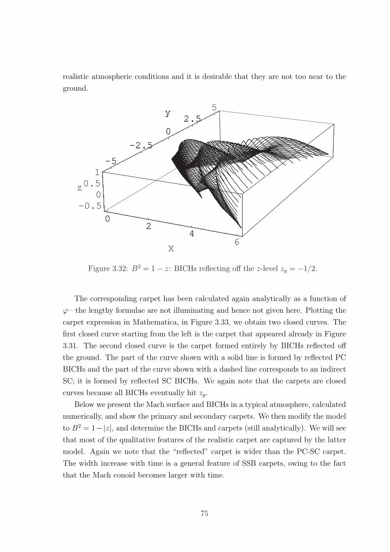
realistic atmospheric conditions and it is desirable that they are not too near to the
ground.
02
46
X
-5
-2.5
02.5
5y
-0.50
0.51
z
02
46
X
-5
-2.5
02.5
5y
Figure 3.32: B2 = 1− z: BICHs reflecting off the z-level zg = −1/2.
The corresponding carpet has been calculated again analytically as a function of
ϕ—the lengthy formulae are not illuminating and hence not given here. Plotting the
carpet expression in Mathematica, in Figure 3.33, we obtain two closed curves. The
first closed curve starting from the left is the carpet that appeared already in Figure
3.31. The second closed curve is the carpet formed entirely by BICHs reflected off
the ground. The part of the curve shown with a solid line is formed by reflected PC
BICHs and the part of the curve shown with a dashed line corresponds to an indirect
SC; it is formed by reflected SC BICHs. We again note that the carpets are closed
curves because all BICHs eventually hit zg.
Below we present the Mach surface and BICHs in a typical atmosphere, calculated
numerically, and show the primary and secondary carpets. We then modify the model
to B2 = 1−|z|, and determine the BICHs and carpets (still analytically). We will see
that most of the qualitative features of the realistic carpet are captured by the latter
model. Again we note that the “reflected” carpet is wider than the PC-SC carpet.
The width increase with time is a general feature of SSB carpets, owing to the fact
that the Mach conoid becomes larger with time.
75
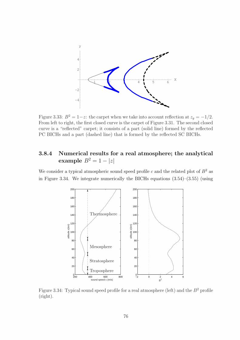
1 2 3 4 5 6X
-4
-2
2
4
y
Figure 3.33: B2 = 1−z: the carpet when we take into account reflection at zg = −1/2.From left to right, the first closed curve is the carpet of Figure 3.31. The second closedcurve is a “reflected” carpet; it consists of a part (solid line) formed by the reflectedPC BICHs and a part (dashed line) that is formed by the reflected SC BICHs.
3.8.4 Numerical results for a real atmosphere; the analyticalexample B2 = 1− |z|
We consider a typical atmospheric sound speed profile c and the related plot of B2 as
in Figure 3.34. We integrate numerically the BICHs equations (3.54)–(3.55) (using
200 400 600 8000
20
40
60
80
100
120
140
160
180
200
sound speed c (m/s)
altit
ude
z(km
)
−2 0 2 4 60
20
40
60
80
100
120
140
160
180
200
B2
altit
ude
z(km
)
Thermosphere
Stratosphere
Mesosphere
Troposphere
Figure 3.34: Typical sound speed profile for a real atmosphere (left) and the B2 profile(right).
76
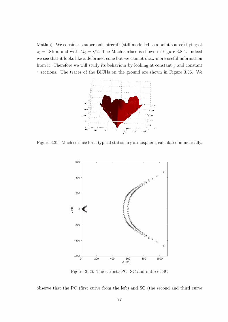
Matlab). We consider a supersonic aircraft (still modelled as a point source) flying at
z0 = 18 km, and with M0 =√
2. The Mach surface is shown in Figure 3.8.4. Indeed
we see that it looks like a deformed cone but we cannot draw more useful information
from it. Therefore we will study its behaviour by looking at constant y and constant
z sections. The traces of the BICHs on the ground are shown in Figure 3.36. We
Figure 3.35: Mach surface for a typical stationary atmosphere, calculated numerically.
0 200 400 600 800 1000−600
−400
−200
0
200
400
600
X (km)
y (k
m)
Figure 3.36: The carpet: PC, SC and indirect SC
observe that the PC (first curve from the left) and SC (the second and third curve
77
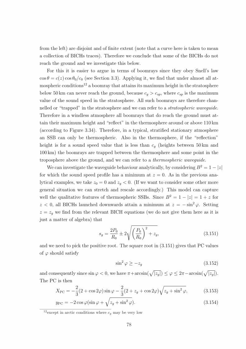
from the left) are disjoint and of finite extent (note that a curve here is taken to mean
a collection of BICHs traces). Therefore we conclude that some of the BICHs do not
reach the ground and we investigate this below.
For this it is easier to argue in terms of boomrays since they obey Snell’s law
cos θ = c(z) cos θ0/c0 (see Section 3.3). Applying it, we find that under almost all at-
mospheric conditions12 a boomray that attains its maximum height in the stratosphere
below 50 km can never reach the ground, because cg > csp, where csp is the maximum
value of the sound speed in the stratosphere. All such boomrays are therefore chan-
nelled or “trapped” in the stratosphere and we can refer to a stratospheric waveguide.
Therefore in a windless atmosphere all boomrays that do reach the ground must at-
tain their maximum height and “reflect” in the thermosphere around or above 110 km
(according to Figure 3.34). Therefore, in a typical, stratified stationary atmosphere
an SSB can only be thermospheric. Also in the thermosphere, if the “reflection”
height is for a sound speed value that is less than cg (heights between 50 km and
100 km) the boomrays are trapped between the thermosphere and some point in the
troposphere above the ground, and we can refer to a thermospheric waveguide.
We can investigate the waveguide behaviour analytically, by consideringB2 = 1− |z|for which the sound speed profile has a minimum at z = 0. As in the previous ana-
lytical examples, we take z0 = 0 and zg < 0. (If we want to consider some other more
general situation we can stretch and rescale accordingly.) This model can capture
well the qualitative features of thermospheric SSBs. Since B2 = 1 − |z| = 1 + z for
z < 0, all BICHs launched downwards attain a minimum at z = − sin2 ϕ. Setting
z = zg we find from the relevant BICH equations (we do not give them here as it is
just a matter of algebra) that
sg =2P0
R0
± 2
√(P0
R0
)2
+ zg, (3.151)
and we need to pick the positive root. The square root in (3.151) gives that PC values
of ϕ should satisfy
sin2 ϕ ≥ −zg (3.152)
and consequently since sinϕ < 0, we have π+arcsin(√|zg|) ≤ ϕ ≤ 2π−arcsin(
√|zg|).The PC is then
XPC = −2
3(2 + cos 2ϕ) sinϕ− 2
3(2 + zg + cos 2ϕ)
√zg + sin2 ϕ, (3.153)
yPC = −2 cosϕ(sinϕ+√zg + sin2 ϕ). (3.154)
12except in arctic conditions where cg may be very low
78
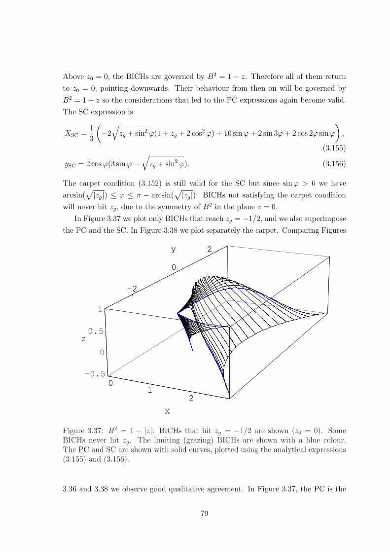
Above z0 = 0, the BICHs are governed by B2 = 1 − z. Therefore all of them return
to z0 = 0, pointing downwards. Their behaviour from then on will be governed by
B2 = 1 + z so the considerations that led to the PC expressions again become valid.
The SC expression is
XSC =1
3
(−2
√zg + sin2 ϕ(1 + zg + 2 cos2 ϕ) + 10 sinϕ+ 2 sin 3ϕ+ 2 cos 2ϕ sinϕ
),
(3.155)
ySC = 2 cosϕ(3 sinϕ−√zg + sin2 ϕ). (3.156)
The carpet condition (3.152) is still valid for the SC but since sinϕ > 0 we have
arcsin(√|zg|) ≤ ϕ ≤ π − arcsin(
√|zg|). BICHs not satisfying the carpet condition
will never hit zg, due to the symmetry of B2 in the plane z = 0.
In Figure 3.37 we plot only BICHs that reach zg = −1/2, and we also superimpose
the PC and the SC. In Figure 3.38 we plot separately the carpet. Comparing Figures
01
2
X
-2
0
2y
-0.5
0
0.5
1
z
01
2
X
-2
0
2y
Figure 3.37: B2 = 1 − |z|: BICHs that hit zg = −1/2 are shown (z0 = 0). SomeBICHs never hit zg. The limiting (grazing) BICHs are shown with a blue colour.The PC and SC are shown with solid curves, plotted using the analytical expressions(3.155) and (3.156).
3.36 and 3.38 we observe good qualitative agreement. In Figure 3.37, the PC is the
79
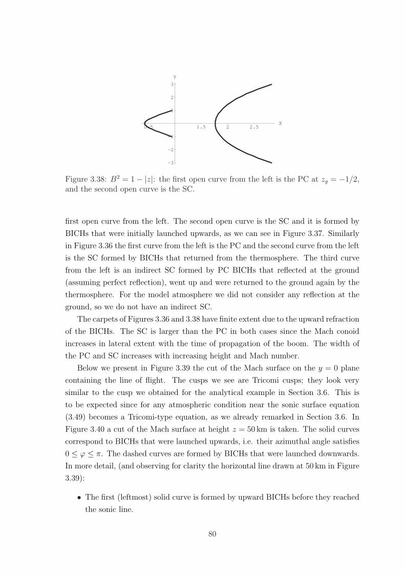
0.5 1.5 2 2.5X
-3
-2
-1
1
2
3
y
Figure 3.38: B2 = 1− |z|: the first open curve from the left is the PC at zg = −1/2,and the second open curve is the SC.
first open curve from the left. The second open curve is the SC and it is formed by
BICHs that were initially launched upwards, as we can see in Figure 3.37. Similarly
in Figure 3.36 the first curve from the left is the PC and the second curve from the left
is the SC formed by BICHs that returned from the thermosphere. The third curve
from the left is an indirect SC formed by PC BICHs that reflected at the ground
(assuming perfect reflection), went up and were returned to the ground again by the
thermosphere. For the model atmosphere we did not consider any reflection at the
ground, so we do not have an indirect SC.
The carpets of Figures 3.36 and 3.38 have finite extent due to the upward refraction
of the BICHs. The SC is larger than the PC in both cases since the Mach conoid
increases in lateral extent with the time of propagation of the boom. The width of
the PC and SC increases with increasing height and Mach number.
Below we present in Figure 3.39 the cut of the Mach surface on the y = 0 plane
containing the line of flight. The cusps we see are Tricomi cusps; they look very
similar to the cusp we obtained for the analytical example in Section 3.6. This is
to be expected since for any atmospheric condition near the sonic surface equation
(3.49) becomes a Tricomi-type equation, as we already remarked in Section 3.6. In
Figure 3.40 a cut of the Mach surface at height z = 50 km is taken. The solid curves
correspond to BICHs that were launched upwards, i.e. their azimuthal angle satisfies
0 ≤ ϕ ≤ π. The dashed curves are formed by BICHs that were launched downwards.
In more detail, (and observing for clarity the horizontal line drawn at 50 km in Figure
3.39):
• The first (leftmost) solid curve is formed by upward BICHs before they reached
the sonic line.
80
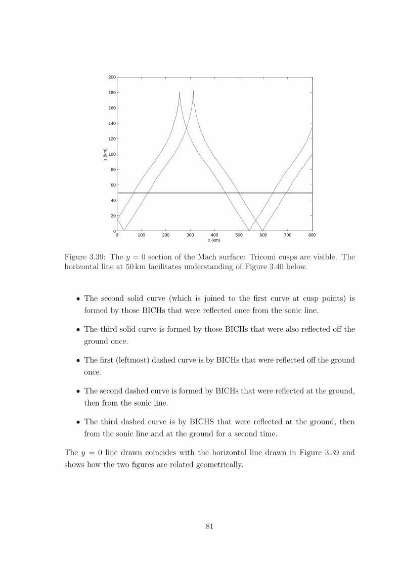
����
0 100 200 300 400 500 600 700 8000
20
40
60
80
100
120
140
160
180
200
x (km)
z (k
m)
Figure 3.39: The y = 0 section of the Mach surface: Tricomi cusps are visible. Thehorizontal line at 50 km facilitates understanding of Figure 3.40 below.
• The second solid curve (which is joined to the first curve at cusp points) is
formed by those BICHs that were reflected once from the sonic line.
• The third solid curve is formed by those BICHs that were also reflected off the
ground once.
• The first (leftmost) dashed curve is by BICHs that were reflected off the ground
once.
• The second dashed curve is formed by BICHs that were reflected at the ground,
then from the sonic line.
• The third dashed curve is by BICHS that were reflected at the ground, then
from the sonic line and at the ground for a second time.
The y = 0 line drawn coincides with the horizontal line drawn in Figure 3.39 and
shows how the two figures are related geometrically.
81
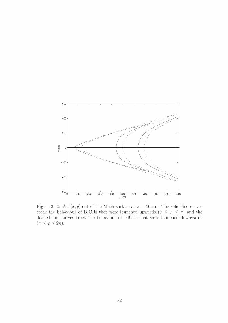
0 100 200 300 400 500 600 700 800 900 1000−600
−400
−200
0
200
400
600
x (km)
y (k
m)
Figure 3.40: An (x, y)-cut of the Mach surface at z = 50 km. The solid line curvestrack the behaviour of BICHs that were launched upwards (0 ≤ ϕ ≤ π) and thedashed line curves track the behaviour of BICHs that were launched downwards(π ≤ ϕ ≤ 2π).
82
3.9 Focusing
In this section we discuss focusing of sound waves and weak shock waves in general,
consider some particular examples, and outline similarities and differences.
The word caustic13 was adopted by Airy in 1838 to describe regions of light focus-
ing [4]. An acoustical caustic is similarly a region of sound focusing. In the physical
world the amplitude of light or sound at a caustic may be an order of magnitude larger
than in any other region of the wavefield. Therefore caustics are desirable in appli-
cations where focusing of waves provides a benefit, e.g. in medical procedures such
as ESWL (Extracorporeal Shock Wave Lithotripsy—the breaking of kidney stones by
focusing shock waves [105]), but they are obviously an undesirable side effect in the
sonic boom context.
An optical or acoustical caustic can be defined as an envelope of optical or acoustic
rays (in the framework of GA or GO); there adjacent rays meet. At an envelope the ray
tube area becomes zero [94] and the hence the amplitude predicted by GA is infinite.
(It is a standard result of GA that the wavefield intensity is inversely proportional to
the ray tube area.)
We consider a two-parameter family of rays labelled with parameters s1, s2 and t
is the parameter along the rays. It can be shown formally that the ray tube area is
proportional to the Jacobian of the transformation between the spatial coordinates
and the ray parameters, given by
J(s1, s2, t) =∂(x1, x2, x3)
∂(s1, s2, t). (3.157)
(See, for instance, [68].) Therefore when J = 0, the ray tube area is zero and a
caustic can be alternatively defined as the locus of points for which J = 0. Caustics
are therefore also the singularities of the map from the space coordinates to the ray
parameters and hence sets of co-dimension 1; this means that in three dimensions they
are surfaces and in two dimensions they are curves [68]. (This has been illustrated in
all the examples we have seen previously.)
An infinite amplitude at the caustic obviously cannot agree with physical observa-
tions. This discrepancy of GA with the physical world indicates that the assumption
on which GA is built, namely that the local gradients of the wavenumber are small
(or equivalently that diffraction is negligible), breaks down.
However, even though GA fails to predict the correct amplitude at a caustic, it
still accurately predicts the location and geometry of the caustics. This is true both
13the word comes from the greek word “kaiein” meaning “burning”.
83
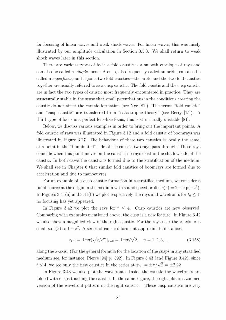
for focusing of linear waves and weak shock waves. For linear waves, this was nicely
illustrated by our amplitude calculation in Section 3.5.3. We shall return to weak
shock waves later in this section.
There are various types of foci: a fold caustic is a smooth envelope of rays and
can also be called a simple focus. A cusp, also frequently called an arete, can also be
called a superfocus, and it joins two fold caustics—the arete and the two fold caustics
together are usually referred to as a cusp caustic. The fold caustic and the cusp caustic
are in fact the two types of caustic most frequently encountered in practice. They are
structurally stable in the sense that small perturbations in the conditions creating the
caustic do not affect the caustic formation (see Nye [81]). The terms “fold caustic”
and “cusp caustic” are transferred from “catastrophe theory” (see Berry [15]). A
third type of focus is a perfect lens-like focus; this is structurally unstable [81].
Below, we discuss various examples in order to bring out the important points. A
fold caustic of rays was illustrated in Figure 3.12 and a fold caustic of boomrays was
illustrated in Figure 3.27. The behaviour of these two caustics is locally the same:
at a point in the “illuminated” side of the caustic two rays pass through. These rays
coincide when this point moves on the caustic; no rays exist in the shadow side of the
caustic. In both cases the caustic is formed due to the stratification of the medium.
We shall see in Chapter 6 that similar fold caustics of boomrays are formed due to
acceleration and due to manoeuvres.
For an example of a cusp caustic formation in a stratified medium, we consider a
point source at the origin in the medium with sound speed profile c(z) = 2−exp(−z2).
In Figures 3.41(a) and 3.41(b) we plot respectively the rays and wavefronts for t0 ≤ 1;
no focusing has yet appeared.
In Figure 3.42 we plot the rays for t ≤ 4. Cusp caustics are now observed.
Comparing with examples mentioned above, the cusp is a new feature. In Figure 3.42
we also show a magnified view of the right caustic. For the rays near the x-axis, z is
small so c(z) ≈ 1 + z2. A series of caustics forms at approximate distances
xCn = ±nπ(√c/c′′)|z=0 = ±nπ/
√2, n = 1, 2, 3, ... (3.158)
along the x-axis. (For the general formula for the location of the cusps in any stratified
medium see, for instance, Pierce [94] p. 392). In Figure 3.43 (and Figure 3.42), since
t ≤ 4, we see only the first caustics in the series at xC1 = ±π/√2 = ±2.22.
In Figure 3.43 we also plot the wavefronts. Inside the caustic the wavefronts are
folded with cusps touching the caustic. In the same Figure, the right plot is a zoomed
version of the wavefront pattern in the right caustic. These cusp caustics are very
84
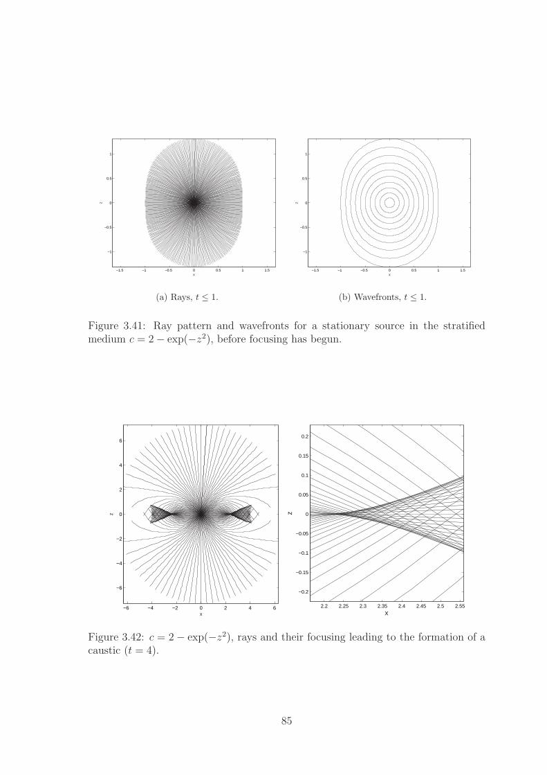
−1.5 −1 −0.5 0 0.5 1 1.5
−1
−0.5
0
0.5
1
x
z
(a) Rays, t ≤ 1.
−1.5 −1 −0.5 0 0.5 1 1.5
−1
−0.5
0
0.5
1
x
z(b) Wavefronts, t ≤ 1.
Figure 3.41: Ray pattern and wavefronts for a stationary source in the stratifiedmedium c = 2− exp(−z2), before focusing has begun.
−6 −4 −2 0 2 4 6
−6
−4
−2
0
2
4
6
x
z
2.2 2.25 2.3 2.35 2.4 2.45 2.5 2.55
−0.2
−0.15
−0.1
−0.05
0
0.05
0.1
0.15
0.2
x
z
Figure 3.42: c = 2− exp(−z2), rays and their focusing leading to the formation of acaustic (t = 4).
85
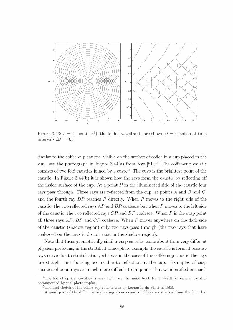
−6 −4 −2 0 2 4 6
−6
−4
−2
0
2
4
6
x
z
2.6 2.8 3 3.2 3.4 3.6 3.8 4
−0.8
−0.6
−0.4
−0.2
0
0.2
0.4
0.6
0.8
xz
Figure 3.43: c = 2− exp(−z2), the folded wavefronts are shown (t = 4) taken at timeintervals ∆t = 0.1.
similar to the coffee-cup caustic, visible on the surface of coffee in a cup placed in the
sun—see the photograph in Figure 3.44(a) from Nye [81].14 The coffee-cup caustic
consists of two fold caustics joined by a cusp.15 The cusp is the brightest point of the
caustic. In Figure 3.44(b) it is shown how the rays form the caustic by reflecting off
the inside surface of the cup. At a point P in the illuminated side of the caustic four
rays pass through. Three rays are reflected from the cup, at points A and B and C,
and the fourth ray DP reaches P directly. When P moves to the right side of the
caustic, the two reflected rays AP and BP coalesce but when P moves to the left side
of the caustic, the two reflected rays CP and BP coalesce. When P is the cusp point
all three rays AP , BP and CP coalesce. When P moves anywhere on the dark side
of the caustic (shadow region) only two rays pass through (the two rays that have
coalesced on the caustic do not exist in the shadow region).
Note that these geometrically similar cusp caustics come about from very different
physical problems; in the stratified atmosphere example the caustic is formed because
rays curve due to stratification, whereas in the case of the coffee-cup caustic the rays
are straight and focusing occurs due to reflection at the cup. Examples of cusp
caustics of boomrays are much more difficult to pinpoint16 but we identified one such
14The list of optical caustics is very rich—see the same book for a wealth of optical causticsaccompanied by real photographs.
15The first sketch of the coffee-cup caustic was by Leonardo da Vinci in 1508.16A good part of the difficulty in creating a cusp caustic of boomrays arises from the fact that
86
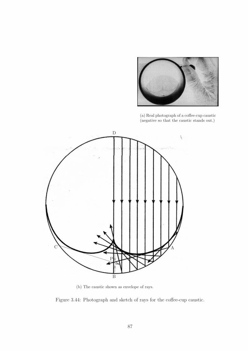
(a) Real photograph of a coffee-cup caustic(negative so that the caustic stands out.)
A
B
P
C
D
(b) The caustic shown as envelope of rays.
Figure 3.44: Photograph and sketch of rays for the coffee-cup caustic.
87
scenario, which can still be treated analytically. It will be discussed at the end of
Chapter 6.
In all the examples of caustics mentioned above the difference in the number of
rays across the caustic is exactly two. This is in fact a generic feature of all caustics
(see Lighthill [72], Section 4.11, p. 385).
The remedy for the infinity of the wavefield predicted by GA at caustics has
been the subject of intensive research, both for linear and nonlinear waves. The
discrepancy between the physical world and GA predictions is due to diffraction,
nonlinearity, dissipation and other effects that are not accounted for in the latter.
Assuming that diffraction effects are more important than the other neglected
effects in the neighbourhood of the caustic, for linear monochromatic waves Buchal
and Keller [19] and Ludwig [75] constructed the Geometrical Theory of Diffraction
(GTD), which recovers diffraction effects to first order in an appropriately defined
neighbourhood of the caustic, usually called the Diffraction Boundary Layer (DBL).
It turns out that the consistent approximation of the Euler equations in the DBL
is the linear Tricomi equation. The generic solution of the Tricomi equation for
monochromatic waves is the Airy function. The solution in the DBL is then matched
to the GA solution outside of the DBL.
Focusing may arise as an undesirable consequence of a supersonic flight. Focusing
of the shock waves can have one or more of three causes:
1. Because the flight takes place in a non-uniform medium—a very likely scenario
especially for SSBs and it is what we have concentrated on in this chapter.
2. Because the aircraft in every supersonic flight has to accelerate through the
sound speed (but maybe also during other parts of the flight). This focusing is
further discussed in Chapter 6; it will be shown that for constant acceleration
in a uniform medium again a fold caustic of boomrays arises. We will also see
there that a cusp caustic of boomrays arises when the same motion takes place
in the stratified atmosphere c = 1/√
1− z.
3. Because of other manoeuvres such as turns. Examples of various manoeuvres
are also discussed in Chapter 6.
Flight tests [123, 47] suggest that the caustics that arise in sonic boom focusing are
mainly fold caustics and much more rarely cusp caustics [76]. (Cusp caustics have
only been documented in the flight tests by Wanner et al. in [123].) The primary
boomrays are always emitted at a fixed angle dictated by the boomray condition.
88
sonic boom enhancement factors observed are two to five times for a fold caustic and
can be up to ten for a cusp caustic.
In sonic boom problems we are interested in the caustics of boomrays, rather than
caustics of ordinary rays, but the local geometrical features of the former and the latter
case are the same, as indicated by catastrophe theory [15] and as illustrated through
the examples in this thesis. For weak shocks, experimental work by Sturtevant and
Kulkarny [118] and by Marchiano et al. [77] supports the belief that deviation caused
to the caustics’ geometry by nonlinearity is negligible. Therefore geometrical results
from linear waves are still accepted as relevant. It is believed, however, that in
order to predict the correct amplitudes near caustics diffraction effects have to be
complemented by nonlinear effects; we elaborate on this below.
When the wave incident on a fold caustic is a shock, the solution of the linear
Tricomi equation is singular; an incoming double-shock N -wave is transformed into
the so-called U -wave with two infinite peaks (this U -wave can be derived as the
Hilbert transform of the N -wave —see article [109] by Rosales and Tabak). This is
an unphysical result.
For a correct estimation of the associated wavefield at a fold caustic it seems that
nonlinear effects need to be retained as a limiting mechanism. This assertion is sup-
ported again by the laboratory-scale experiments of Sturtevant and Kulkarny [118]
and of Marchiano et al. [78]. When retaining both diffraction and nonlinear effects
near fold caustics of weak shocks the nonlinear Tricomi equation (z + ΦX)ΦXX = Φzz
arises as the consistent approximation of the Euler equations. The latter equation
was first derived by Guiraud in 1965 [45], and again by Hayes in 1968 [53]. Pechuzal
and Kevorkian [91] arrived at the same equation when they studied the focusing of
shocks created by a supersonic source in a weakly stratified linear wind and in a two-
dimensional uniform atmosphere. Similar equations were subsequently derived by
Fung [41], Rosales and Tabak [109], and Auger [10]. Numerical solutions of the non-
linear Tricomi equation for a single shock were provided by the approximate method
of the hodograph transform by Seebass [113], Gill and Seebass [43], and Fung [41]. By
2002, Cheng and Hafez [23] and many others had devised other numerical methods for
solving the nonlinear Tricomi equation. A faster and more robust numerical method
was introduced by Auger and Coulouvrat [11] in 2002. In 2003, Marchiano, Coulou-
vrat and Grenon in [77] applied this method to an incident N -wave for estimating
the amplitudes created by acceleration through the sound speed at the ground track,
using the Eurosup configuration derived from the European configuration for a future
SST [37], in realistic atmospheric conditions.
89
On the other hand, for the wavefield at a cusp caustic, much less research has been
done [29, 28, 25]. In the linear theory the generic function describing the solution at
a cusp is the Pearcey function [90]. For an incoming shock wave the outgoing wave
has again infinite singularities; the idea for remedial action is the same as for the fold
caustic, that is by introducing nonlinearity as a limiting mechanism. The most recent
work is by Coulouvrat [25]; he proposes that the KZ equation should be solved in the
vicinity of the cusp and provides a description of how a numerical scheme could be
developed to handle an incoming N -wave.
3.10 Sonic booms in an atmosphere with wind
Waves in fluids are generally affected by any underlying motion of the fluid, such as
winds in the atmosphere or currents in the ocean. Below we will present briefly the
theory of GA in a moving medium [17, 65, 87] in order to determine how atmospheric
winds influence the SSB propagation. We consider a non-uniform background flow of
the form U(x) = (U1(x), U2(x), U3(x)), taking place in a slowly varying atmosphere.
We assume that the length-scale of variation of the ambient flow is much larger than
the wavelength and therefore U(x) is slowly varying. This assumption is necessary if
we are to retain the GA framework used for stationary media. Note that from now
on we will refer to the ambient flow as “wind”.
The ray equations valid in a moving medium are the ordinary differential equations
x =∂ω
∂k, k = −∂ω
∂x, (3.159)
which are valid for any waves with the general dispersion relation ω = ω(k;x) (see
Lighthill [72], equations (106)–(107) and the discussion on ray tracing in a wind, pp.
325–334). For sound waves in a stationary medium the local dispersion relation is
ωr = c(x)|k|, as we already noted in (3.32). The subscript r applied here stands
for rest or relative because ωr is the frequency of the waves relative to the ambient
flow velocity. For sound waves in a moving medium the local dispersion relation is
modified to
ω(k;x) = ωr(k) + U(x).k = c(x)|k|+ U(x).k, (3.160)
and therefore equations (3.159) become
dxidt
= Ui +∂ωr∂ki
= Ui + cni, (3.161)
dkidt
= −kj ∂Uj∂xi
− ∂ωr∂xi
= −kj ∂Uj∂xi
− ∂c
∂xi|k|. (3.162)
90
Since n = k/|k| the system of equations (3.161)–(3.162) is closed. The right-hand
side of (3.161) is the vector sum of the wind velocity and the direction vector of
the ray when the fluid is at rest. The first term in the right-hand side of (3.162)
represents refraction due to the gradients of the wind and the second term refraction
due to gradients of the sound speed.
For typical atmospheric conditions the wind is in many cases approximately hori-
zontal. We show below, generalising Lighthill’s treatment in [72] for U = (U(z), 0, 0)
to the case of U = (U(z), V (z), 0), whose magnitude and direction varies with height,
and a stratified atmosphere we can derive a generalised Snell’s law. Firstly, from the
dispersion relation (3.160), and letting k = −(p, q, r) = (k, l,m), we have
ω(k;x) = c|k|+ kU(z) + lV (z). (3.163)
For a medium stratified in the z-direction equations (3.162) give that k and l are con-
stant; since the changes are only in the z-direction only the component m changes.
Furthermore ω is constant along a ray, since the derivative of ω along a ray isdω
dt=∂ω
∂xi
dxidt
+∂ω
∂ki
dkidt
= 0 (using equations (3.161) and (3.162)—see also [72], p.
319.) We then take
k = kH cosψ, l = kH sinψ, m = kH cotϑ, (3.164)
where kH =√k2 + l2, ψ is the constant azimuthal angle to the wind direction, and
ϑ is the variable angle to the z-direction; we find that (3.163) then becomes the
generalised Snell’s law
c(z)
sinϑ+ U(z) cosψ + V (z) sinψ =
ω
kH= constant
⇒ sinϑ =c(z)
ωk−1H − U(z) cosψ − V (z) sinψ
. (3.165)
When we take U = V = 0 and ϑ 7→ π/2 − θ we recover (3.35), the Snell’s law in a
stationary medium.
Relation (3.165) is very important because it can explain how a stratospheric SSB
may arise. For a boomray to be reflected from a height z = zr in the stratosphere
and then reach the ground, setting V = 0 in (3.165), we find that the condition
cosψ(U(zr)− Ug) > cg − c(zr) (3.166)
should be satisfied, where cg is the ground sound speed and c(zr), the sound speed
at the reflection height. This means that the difference in the wind speed between
91
the reflection height and the ground must be large enough in the direction of the
boomray so that it compensates for the fact that cg is greater than c(zr).
Note that from (3.163) we can write down
m(z) = ±√(
ω − kU(z)
c(z)
)2
− k2 − l2 (3.167)
and equations (3.161) give
dy
dz=
∂ωr/∂l
∂ωr/∂m,
dx
dz=U(z) + ∂ωr/∂k
∂ωr/∂m, (3.168)
where the right-hand sides are known functions of z and when integrated give the
projections of the rays in the x and y plane respectively. This is not so useful for rays
that go through a reflection point where m changes sign, and solving the ordinary
differential equations directly is preferable.
For the most part in this chapter we have investigated the geometry of thermo-
spheric SSBs and in this section we looked at stratospheric SSBs. It is also important
to know what is the intensity associated with these two types of SSBs. This issue has
been addressed within the SOBER programme, and it has been briefly discussed in
the Introduction.
The link with the BICHs
There is still an interesting point to make here, as promised on page 73: If we take
U to be a constant (and the medium stratified in the z-direction) equations (3.161)-
(3.162) reduce to the equations for the BICH (3.54)–(3.55). Therefore the BICHs can
be thought of as the rays in a medium with a “supersonic” stream (U, 0, 0) and they
satisfy the generalised Snell’s law (3.165). (We no longer call (U, 0, 0) the “wind”
because wind is never supersonic.)
3.11 Other considerations
The well-defined impact areas shown in our simple models do not really materialise
in real atmospheric conditions; variations in the atmospheric wind and temperature
profiles may cause drastic changes to the character of the carpets.
Furthermore, in reality, the atmospheric parameters are given as data points sam-
pled or predicted in certain intervals of time and at certain locations on the ground.
Therefore the necessary interpolation needed to produce a smooth profile for the
ambient properties of the atmosphere, such as temperature or pressure, inevitably
introduces errors that may change the character of the computed carpet.
92
3.12 Summary and conclusions
In this chapter, we have first detailed the terms frequently used in sonic boom re-
search. We presented a series of mainly analytical examples which showed how rays
and boomrays arise as a means for studying long-range sound and sonic boom prop-
agation in a non-uniform atmosphere. For the main part we looked at stationary
media. In particular we illustrated a fold caustic of rays and a fold caustic of boom-
rays and in the latter case we have shown how this corresponds to a Tricomi cusp
on the Mach envelope. The Mach envelope parts joining to each other through this
Tricomi cusp were called “incident” and “reflected”. We shall see in Chapter 6 that
we can use the same labelling for the Mach envelope arising in acceleration through
the sound speed.
For our three-dimensional examples we worked in the aerodynamic frame and
traced the BICHs rather than the boomrays. This is an alternative, simpler, way to
follow the boom in the case of steady level flight. In particular, the analytical example
with B2 = 1− |z| gave carpets qualitatively similar to those in a typical atmosphere.
Throughout the chapter we concentrated on the geometrical features of propaga-
tion, except in Section 3.5.3 where we have calculated the amplitude due to a sta-
tionary monochromatic source in the medium with sound speed profile c = 1/√
1− z.
In that example we have compared the full linear wave theory with the Geometrical
Theory of Diffraction: we have shown that an order 1 wavefield exists inside the fold
caustic z = 1−x2/4 where ray theory predicts two rays passing through each point, a
larger amplitude exists near the caustic where the rays coalesce, and an exponentially
decaying wavefield exists outside the caustic as also predicted by GTD. (Work on the
amplitudes related to focusing will also be presented in Chapters 6 and 7.)
We have also discussed similarities and differences in the focusing of linear waves
and weak shock waves, and related this discussion to our examples. Finally, we looked
at ray tracing in a wind as a means for explaining stratospheric secondary booms.
93
Chapter 4
Steady supersonic flow in auniform atmosphere
4.1 Introduction
In this chapter we are going to investigate the flow around aerofoils, moving at a
constant supersonic speed (−U, 0, 0) in a stationary uniform medium. The equations
of motion are taken to be the Euler equations, as detailed in Chapter 2. This is a
good approximation in most of the flow; we will neglect viscous and thermal effects
which are confined to boundary layers around the body.
The chapter is structured as follows: firstly, the Euler equations are recast, under
certain assumptions, into a scalar nonlinear equation for the velocity potential. Sub-
sequently, the method of Matched Asymptotic Expansions (MAE) is used to derive
consistent approximations of the potential equation near the aerofoil (near-field) and
far from the aerofoil (far-field), in two and three dimensions. In the near-field a linear
wave equation is derived at leading order. However, the linear approximation breaks
down in the far-field due to small nonlinear effects that cumulatively become impor-
tant there. In the far-field the consistent approximation of the potential equation at
leading order is a so-called “Kinematic Wave Equation”. Solving the latter equation
determines the characteristics and shocks.
That the nonlinearities are important in the far-field is a well-known result in sonic
boom research. In 1952 Whitham, in [124], used an ingenuous geometrical approach
to include these nonlinearities. He created the so called “quasi-linear” theory based
upon the hypothesis that the linear theory yields the correct values of perturbations
along the characteristics as long as these characteristics are shifted appropriately in
the far-field. These modified characteristics incorporate at leading order the effect
of nonlinearity. Eventually the shifting of characteristics leads to their crossing, and
94
shocks have to be introduced to resolve the resulting multi-valued regions. On the
other hand, Hayes in [51] derived the correct KWE at the far-field for planar bodies
and bodies of revolution, but he did not employ formal asymptotic methods; he
neglected terms in a somewhat ad hoc way based on physical intuition. However, the
advantage of our asymptotic analysis here is that it is systematic and does not need
to rely on such physical arguments. 1 Furthermore, it provides us with the means to
calculate the higher orders, should we wish to do so.
4.2 Euler equations for steady flow
We define the Mach number of the aerofoil as M0 = U/c0 > 1 and the local Mach
number of the flow as M = |u|/c0. For an aerofoil with M0 ¿ 1 (typically less than
0.3) the compressibility effects are usually negligible to first order and the flow is
called incompressible. The flow is said to be compressible for larger values of M0. It
is called subsonic or supersonic if the flow velocity relative to the aerofoil is subsonic or
supersonic everywhere; it is called transonic if there are both subsonic and supersonic
regions: for typical aerofoils the subsonic regime is for M0 from about 0.8 to 1.2. Note
that for M0 greater than about 5 the flow is called hypersonic. The exact cutoff values
of M0 are dependent on the particular configuration. In this thesis, the Mach number
M0 will always be large enough for compressibility effects to play an important role
but we will not consider hypersonic flows.
It is convenient to work in the aerodynamic frame in which the aerofoil is station-
ary and there is an incident supersonic stream (U, 0, 0). By defining the travelling
coordinate X = x+Ut, the problem becomes time-independent, and the Euler equa-
tions (2.4), (2.5) and (2.12) simplify to
∇ . (ρu) = 0, (4.1)
∇ p+ ρ (u ·∇)u = 0, (4.2)
u.∇S = 0 or u.∇ p = c2u.∇ ρ, (4.3)
for a smooth flow. Equation (4.3) gives that the entropy is constant along streamlines
(fluid particle paths and streamlines coincide in steady flow). Furthermore, to a good
approximation air is a polytropic gas (with γ = 1.4), so c2 = γp/ρ and (4.3) becomes
ρu.∇ p = γpu.∇ ρ. (4.4)
1Our MAE framework in two dimensions is very similar to that in Van Dyke [121] but MAEframework in three dimensions is more original.
95
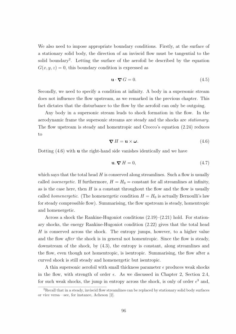
We also need to impose appropriate boundary conditions. Firstly, at the surface of
a stationary solid body, the direction of an inviscid flow must be tangential to the
solid boundary2. Letting the surface of the aerofoil be described by the equation
G(x, y, z) = 0, this boundary condition is expressed as
u ·∇G = 0. (4.5)
Secondly, we need to specify a condition at infinity. A body in a supersonic stream
does not influence the flow upstream, as we remarked in the previous chapter. This
fact dictates that the disturbance to the flow by the aerofoil can only be outgoing.
Any body in a supersonic stream leads to shock formation in the flow. In the
aerodynamic frame the supersonic streams are steady and the shocks are stationary.
The flow upstream is steady and homentropic and Crocco’s equation (2.24) reduces
to
∇H = u× ω. (4.6)
Dotting (4.6) with u the right-hand side vanishes identically and we have
u.∇H = 0, (4.7)
which says that the total head H is conserved along streamlines. Such a flow is usually
called isoenergetic. If furthermore, H = H0 = constant for all streamlines at infinity,
as is the case here, then H is a constant throughout the flow and the flow is usually
called homenergetic. (The homenergetic condition H = H0 is actually Bernoulli’s law
for steady compressible flow). Summarising, the flow upstream is steady, homentropic
and homenergetic.
Across a shock the Rankine-Hugoniot conditions (2.19)–(2.21) hold. For station-
ary shocks, the energy Rankine-Hugoniot condition (2.22) gives that the total head
H is conserved across the shock. The entropy jumps, however, to a higher value
and the flow after the shock is in general not homentropic. Since the flow is steady,
downstream of the shock, by (4.3), the entropy is constant, along streamlines and
the flow, even though not homentropic, is isentropic. Summarising, the flow after a
curved shock is still steady and homenergetic but isentropic.
A thin supersonic aerofoil with small thickness parameter ε produces weak shocks
in the flow, with strength of order ε. As we discussed in Chapter 2, Section 2.4,
for such weak shocks, the jump in entropy across the shock, is only of order ε3 and,
2Recall that in a steady, inviscid flow streamlines can be replaced by stationary solid body surfacesor vice versa—see, for instance, Acheson [2].
96
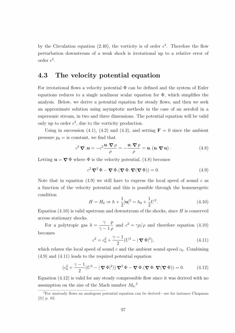
by the Circulation equation (2.40), the vorticity is of order ε3. Therefore the flow
perturbation downstream of a weak shock is irrotational up to a relative error of
order ε2.
4.3 The velocity potential equation
For irrotational flows a velocity potential Φ can be defined and the system of Euler
equations reduces to a single nonlinear scalar equation for Φ, which simplifies the
analysis. Below, we derive a potential equation for steady flows, and then we seek
an approximate solution using asymptotic methods in the case of an aerofoil in a
supersonic stream, in two and three dimensions. The potential equation will be valid
only up to order ε2, due to the vorticity production.
Using in succession (4.1), (4.2) and (4.3), and setting F = 0 since the ambient
pressure p0 = is constant, we find that
c2 ∇ .u = −c2u.∇ ρ
ρ= −u.∇ p
ρ= u. (u.∇u) . (4.8)
Letting u = ∇ Φ where Φ is the velocity potential, (4.8) becomes
c2 ∇2 Φ−∇ Φ.(∇ Φ.∇(∇ Φ)) = 0. (4.9)
Note that in equation (4.9) we still have to express the local speed of sound c as
a function of the velocity potential and this is possible through the homenergetic
condition
H = H0 ⇒ h+1
2|u|2 = h0 +
1
2U2. (4.10)
Equation (4.10) is valid upstream and downstream of the shocks, since H is conserved
across stationary shocks.
For a polytropic gas h =γ
γ − 1
p
ρand c2 = γp/ρ and therefore equation (4.10)
becomes
c2 = c20 +γ − 1
2(U2 − |∇ Φ|2), (4.11)
which relates the local speed of sound c and the ambient sound speed c0. Combining
(4.9) and (4.11) leads to the required potential equation
(c20 +γ − 1
2(U2 − |∇ Φ|2)) ∇2 Φ−∇ Φ.(∇ Φ.∇(∇ Φ)) = 0. (4.12)
Equation (4.12) is valid for any steady compressible flow since it was derived with no
assumption on the size of the Mach number M0.3
3For unsteady flows an analogous potential equation can be derived—see for instance Chapman[21] p. 62.
97
The body boundary condition (4.5) becomes
∇ Φ.nG =∂ Φ
∂n= 0 (4.13)
where nG = ∇G is the normal to the aerofoil surface G = 0. The condition at
infinity can be written as
∇ Φ → (U, 0, 0) as x→ −∞. (4.14)
Once Φ is determined, all flow quantities can be obtained. An expression for pressure
in terms of Φ can be found by combining (4.11) and c2 = γp/ρ, where ρ = (p/κ)1/γ
from the constant entropy condition (2.13) (valid here up to O(ε2)):
p = p0
(1 +
γ − 1
2c20(U2 − |∇ Φ|2)
) γγ−1
. (4.15)
Once we have obtained p we can go back to (2.13) to obtain ρ. We can obtain
T = p/Rρ, using the equation of state (2.8).
4.4 Two-dimensional supersonic flow
In this section we apply the steady supersonic flow theory presented above to the
analysis of the flow around a two-dimensional thin aerofoil in a uniform supersonic
stream. This analysis is applicable for
(a) flows in which conditions are identical in sections parallel to the (x, z)-plane,
such as certain portions of wings (see Figure 4.1).
(b) flows around surfaces of any shape with their (x, z)-section varying only slowly
with y. The flow is then almost identical in every (x, z)-plane. Case (a) is a
special case of this.
We take an aerofoil symmetric with respect to the x-axis. We can then examine all
the essential features of the flow by looking only in the half-plane z > 0. A symmetric
geometry is non-lifting but the analysis that we will present can be easily extended to
lifting aerofoils with asymmetric effects due to light camber and/or non zero, small,
angle of attack (see, for instance, Chapman [21], pp. 145–151). Using cartesian
coordinates x and z we consider an aerofoil profile z = ±G(x). The function G(x) is
usually called the thickness function. We take the chord length to be L, extending
from x = −L/2 to x = L/2, and assume that Gmax ¿ L (see Figure 4.2). Both ends
98
x
y
U
z
Figure 4.1: A body for which the induced supersonic flow can be analysed withtwo-dimensional theory.
L/2G(x)
−L/2
−G(x)
Figure 4.2: An aerofoil with thickness function G(x) and chord L, symmetric withrespect to the x-axis.
of the aerofoil are taken to be pointed. This will lead to the shocks being attached
to the ends of the aerofoil. (If the aerofoil is blunt the shocks will be detached and
stronger and the analysis becomes more complicated.) The thickness ratio of the
aerofoil is defined by
ε =Gmax
L, (4.16)
and it is small, with a typical value of 0.1. We nondimensionalise both x = x/L and
z = z/L and then z(x) = ±εG(x) where G is a fixed O(1) function and −1/2 ≤ x ≤1/2. We will also nondimensionalise all velocities with U , the speed of the incident
supersonic stream. The pressure p is nondimensionalised with its undisturbed value
p0 and ρ with its undisturbed value ρ0. From now on, we will use nondimensional
variables, but we will drop the hats for convenience.
4.4.1 Potential equation
In two dimensions, the potential equation (4.12) becomes
Φzz −B20Φxx = M2
0{γ − 1
2(Φxx + Φzz)(Φ
2x + Φ2
z − 1) + Φxx(Φ2x − 1)+
2ΦxΦzΦxz + Φ2zΦzz}, (4.17)
99
where B0 =√M2
0 − 1 is the Prandtl-Glauert parameter, as already defined in the
previous chapter. On the left-hand side of (4.19) we have the linear wave operator
∂/∂z2 −B20∂/∂x
2 and on the right-hand side all the nonlinear terms.
The aerofoil causes a weak disturbance of order ε to the uniform stream and there-
fore the velocity field is a superposition of the uniform incoming flow
U∞ = (1, 0, 0) and a perturbation velocity field εu′, so that u = U∞+ εu′. Therefore
the potential Φ is written as
Φ = Φ∞ + εφ = x+ εφ. (4.18)
The first term on the right-hand side of (4.18) represents the potential for the uniform
stream U∞ and the perturbation potential φ is for u′ = ∇φ. Inserting (4.18) into
the equation (4.17) and dropping terms of order ε3, we obtain an equation for the
perturbation potential φ:
φzz −B20φxx = εM2
0 {(γ + 1)φxφxx + (γ − 1)φxφzz + 2φzφxz}
+ ε2M20
{γ − 1
2(φxx + φzz)(φ
2x + φ2
z) + φ2zφzz + φ2
xφxx + 2φxφzφxz
}. (4.19)
We also want to express the boundary conditions in terms of φ: since u = Φx =
1+ εφx, v = Φz = 0+ εφz and the normal nG is parallel to (−εG′(x), 1), the boundary
condition (4.13) becomes
φz(x, z)
1 + εφx(x, z)= G′(x) on z = εG(x). (4.20)
The condition at infinity becomes
(φx, φz) → (0, 0) as x→ −∞. (4.21)
4.4.2 Asymptotic analysis
Lowest-order perturbation potential
We tentatively assume the following asymptotic series for the perturbation potential
φ, in integral powers of ε,
φ(x, z, ε) ∼ φ1(x, z) + εφ2(x, z) +O(ε2). (4.22)
Therefore we substitute (4.22) in (4.19) and we equate corresponding powers of ε in
order to determine the equations satisfied by φ1 and φ2. At the lowest order we obtain
φ1zz −B20φ1xx = 0. (4.23)
100
Equation (4.23) is a homogeneous, second-order, wave equation with constant co-
efficients and has two families of characteristics x ± B0z = constant. The general
D’Alembert’s solution in z > 0 is
φ1(x, z) = f(x−B0z) + g(x+B0z) = f(ξ) + g(η), (4.24)
which is a superposition of waves propagating upwards and downwards. Setting
x = t, z = x and B0 = 1/c0 equation (4.24) becomes the familiar equation of one-
dimensional propagation of sound waves, and we can consider linear acoustics and
linear supersonic aerodynamics to be essentially the same subject.
Note that in z < 0 for a symmetric aerofoil the D’Alembert’s solution can be
obtained from (4.24) by taking z 7→ −z i.e. φ1(x, z)|z<0 = f(η) + g(ξ), but for a
general aerofoil a different set of f and g functions would be involved in the solution.
In order to equate corresponding powers of ε we should also transfer the body
boundary condition (4.20) to the axis z = 0. Assuming that φk(x, z) are analytic at
z = 0 we expand in Taylor series about z = 0
φz(x, εG(x)) = φz(x, 0+) + εG(x)φzz(x, 0+) +O(ε2), (4.25)
and similarly for φx(x, εG(x)). Therefore to the lowest order, (4.20) becomes
φ1z(x, 0+) = G′(x). (4.26)
For the lower part of the aerofoil φ1z(x, 0−) = −G′(x) and therefore φ1z has a jump
of 2G′(x) for −1/2 ≤ x ≤ 1/2. There is no jump in φ1z for x > 1/2 or x < −1/2.
The upstream condition at this order is
(φ1x, φ1z) → (0, 0) as x→,−∞. (4.27)
where, from D’ Alembert’s solution (4.24)
φ1x = f ′(ξ) + g′(η), φ1z = −B0f′(ξ) + B0g
′(η), (4.28)
We consider a fixed η = x + B0z characteristic. Letting z → ∞, since η is fixed, we
have x→ −∞. Therefore from (4.27) and (4.28) we get
B0φ1x + φ1z = 2B0g′(η) → 0 ⇒ g → g0 as x→ −∞ and z →∞.
We set g0 = 0, since only the gradient of φ is physically relevant. Therefore
φ1(x, z) = f(ξ). (4.29)
101
A more physical way of arriving at relation (4.29) is to immediately discard the
function g since, by the condition at infinity, only outgoing waves are possible.
Enforcing the boundary condition (4.26) we find f = −G/B0 + f0 where the
constant f0 is also set to zero. Therefore finally
φ1(x, z) = −G(ξ)
B0
= −G(x−B0z)
B0
, (4.30)
i.e. at distance z from the aerofoil φ1 is obtained by translating the function−G(x)/B0
B0z units to the right of the initial condition φ1(x, 0) = −G(x)/B0. The velocity field
(u1, v1) is given as
u1 = φ1x = −G′(ξ)B0
, v1 = φ1z = G′(ξ) = −B0u1. (4.31)
Also in the (nondimensional) pressure relation (4.15), we put Φ = x+ εφ which gives
p =
(1 +
γ − 1
2M2
0 (−2εφx − ε2(φ2x + φ2
z))
)γ/(γ−1)
. (4.32)
Expanding to bring down the exponent γ/(γ − 1), we have
p = 1− γ
2M2
0 (2εφx + ε2(φ2x + φ2
z)) + ε2γM4
0
2φ2x +O(ε3). (4.33)
Assuming the asymptotic expansion p ∼ 1 + εp1 + ε2p2 + O(ε3), from (4.22), the
pressure at the lowest order is
p1 = −γM20φ1x = −γM2
0u1. (4.34)
Now, the nondimensional homentropic flow condition is p = ργ and substituting in it
the asymptotic expansion for p given above, and ρ ∼ 1 + ερ1 + ε2ρ2 + O(ε3), we find
at this order p1 = γρ1. Therefore from (4.34) we find
ρ1 = −M20φ1x = −M2
0u1. (4.35)
We note that
(u1, v1, p1, ρ1) = u1(1,−B0,−γM20 ,−M2
0 ), (4.36)
i.e. the first-order flow variables can all be expressed as a function of u1.
The above analysis is basically the linear Ackeret theory (see, for instance, [121]).
The Ackeret theory is a sufficiently good approximation at and near the body (near-
field). However, it represents disturbances which propagate with undiminished strength
to infinity on the straight, parallel characteristics x ± B0z = constant and fails at
102
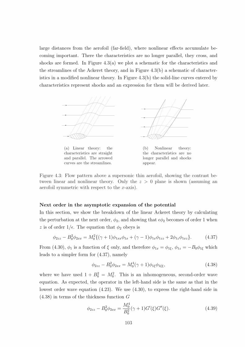
large distances from the aerofoil (far-field), where nonlinear effects accumulate be-
coming important. There the characteristics are no longer parallel, they cross, and
shocks are formed. In Figure 4.3(a) we plot a schematic for the characteristics and
the streamlines of the Ackeret theory, and in Figure 4.3(b) a schematic of character-
istics in a modified nonlinear theory. In Figure 4.3(b) the solid-line curves entered by
characteristics represent shocks and an expression for them will be derived later.
(a) Linear theory: thecharacteristics are straightand parallel. The arrowedcurves are the streamlines.
(b) Nonlinear theory:the characteristics are nolonger parallel and shocksappear.
Figure 4.3: Flow pattern above a supersonic thin aerofoil, showing the contrast be-tween linear and nonlinear theory. Only the z > 0 plane is shown (assuming anaerofoil symmetric with respect to the x-axis).
Next order in the asymptotic expansion of the potential
In this section, we show the breakdown of the linear Ackeret theory by calculating
the perturbation at the next order, φ2, and showing that εφ2 becomes of order 1 when
z is of order 1/ε. The equation that φ2 obeys is
φ2zz −B20φ2xx = M2
0{(γ + 1)φ1xxφ1x + (γ − 1)φ1xφ1zz + 2φ1zφ1xz}. (4.37)
From (4.30), φ1 is a function of ξ only, and therefore φ1x = φ1ξ, φ1z = −B0φ1ξ which
leads to a simpler form for (4.37), namely
φ2zz −B20φ2xx = M4
0 (γ + 1)φ1ξφ1ξξ, (4.38)
where we have used 1 + B20 = M2
0 . This is an inhomogeneous, second-order wave
equation. As expected, the operator in the left-hand side is the same as that in the
lowest order wave equation (4.23). We use (4.30), to express the right-hand side in
(4.38) in terms of the thickness function G
φ2zz −B20φ2xx =
M40
B20
(γ + 1)G′(ξ)G′′(ξ). (4.39)
103
The boundary condition (4.20) at this order gives
φ2z(ξ = x, z = 0+) =1
B0
{B20G(x)G′′(x)− (G′(x))2} when − 1/2 ≤ x ≤ 1/2.
(4.40)
The upstream condition becomes (φ2x, φ2z) → (0, 0) as x→ −∞.
Oblique coordinates; breakdown of the asymptotic expansion
We now change to the oblique coordinates (ξ, z), following Hayes [51] and Van Dyke
[121], p.108. The equation (4.19) for the perturbation potential φ becomes
φzz − 2B0φzξ = εM20{(γ + 1)M2
0φξφξξ + 2(φz − γB0φξ)φξz (4.41)
+ (γ − 1)φξφzz − 2B0φzφξξ}+O(ε2). (4.42)
We can determine the equation satisfied by φ2(ξ, z), either by transforming (4.39) or
by plugging in (4.41) the asymptotic expansion φ = φ1(ξ, z) + εφ2(ξ, z) + O(ε2) and
taking the terms of order ε. We get
φ2zz − 2B0φ2zξ =M4
0
B20
(γ + 1)G′(ξ)G′′(ξ), (4.43)
and it is now clear why changing to oblique coordinates is useful: we can readily
integrate (4.43) with respect to z and obtain the first-order (linear) hyperbolic partial
differential equation
φ2z − 2B0φ2ξ =M4
0
B20
(γ + 1)G′(ξ)G′′(ξ)z + C(ξ), (4.44)
where C(ξ) is an arbitrary function of ξ. We can solve (4.44) with the method
of characteristics.4 The characteristics have constant slope dξ/dz = −2B0 and we
recover the characteristic family
ξ + 2B0z = η = η0 = constant. (4.45)
The variation of φ2 along these characteristics is given by the ordinary differential
equationdφ2
dz=M4
0
B20
(γ + 1)G′(ξ)G′′(ξ)z + C(ξ). (4.46)
From (4.45) we can express ξ = η0 − 2B0z in terms of z and the characteristic label
η0, and (4.46) becomes
dφ2
dz=M4
0
B20
(γ + 1)G′(η0 − 2B0z)G′′(η0 − 2B0z)z + C(η0 − 2B0z). (4.47)
4Van Dyke [121] proceeds instead with an iteration method.
104
Integrating (4.47) with respect to z, we get
φ2(ξ, z) =M4
0 (γ + 1)
B20
∫ z
zG′(η0−2B0z)G′′(η0−2B0z)dz+
∫ z
C(η0−2B0z)dz, (4.48)
and integrating by parts we get
φ2(ξ, z) =M4
0 (γ + 1)
B20
(− z
4B0
(G′(η0 − 2B0z))2 +
1
4B0
∫ z
(G′(η0 − 2B0z))2dz
)
−C1(ξ)
2B0
+ C2(η0).
(4.49)
We have two unknown functions: C1(ξ), which stands for the indefinite integral of
C, and C2(η0). Due to the condition at infinity, C2(η0) must be set to 0 and C1 is
determined below from the body boundary condition
φ2z(ξ = x, 0+)−B0φ2ξ(ξ = x, 0+) =1
B0
{B20G(x)G′′(x)− (G′(x))2}. (4.50)
From (4.49) we obtain the partial derivatives
φ2z = −M40
4B30
(γ + 1)(G′(ξ))2, (4.51)
φ2ξ = −M40
2B30
(γ + 1)G′(ξ)G′′(ξ)z − M40
8B40
(γ + 1)(G′(ξ))2 − 1
2B0
C(ξ), (4.52)
and using them in (4.50), we obtain C in terms of G, G′, G′′ and M0
C(x) = 2B0G(x)G′′(x)− 2
B0
(G′(x))2 +M4
0
4B30
(γ + 1)(G′(x))2. (4.53)
Inserting (4.53) into (4.52) and after some rearrangement, we get the horizontal com-
ponent of the velocity at this order
u2 = φ2ξ = −M40
2B30
(γ + 1)G′(ξ)G′′(ξ)z +G′(ξ)2
B20
(1− M4
0
4B20
(γ + 1)
)−G(ξ)G′′(ξ),
(4.54)
where we assumed the asymptotic expansion u = 1 + εu1 + ε2u2 + O(ε3). The result
(4.54) is in agreement with Van Dyke, (see [121], p. 107, expression (6.24), where this
result was found by iterating on the equation (4.19)), and at the surface, coincides
also with the Busemann solution. From (4.54), the perturbation is
εφ2 ∼ (εz)(γ + 1)M4
0
2B30
(G′)2 (4.55)
105

and therefore εφ2 is of order 1 when (εz) ∼ 1. Therefore, when z ∼ 1/ε, the assumed
asymptotic expansion (4.22) breaks down. Returning to dimensional variables, the
breakdown occurs at a physical distance of order L/ε away from the aerofoil, roughly
10 aerofoil chord lengths away. The breakdown of the asymptotic expansion phys-
ically means that the nonlinear effects that we initially neglected in the near-field
problem become cumulatively significant in the far-field and the nonlinear term φξφξξ
in (4.41) can no longer be neglected. Hayes, in [51], included these nonlinear effects
and derived the appropriate nonlinear equation using physical reasoning. In the next
section we will follow a mathematically systematic approach, consistently modifying
our asymptotic analysis in order to remedy the non-uniformity (4.55) of the asymp-
totic expansion (4.22) and derive the relevant equation valid in the far-field.
4.4.3 Far-field: Kinematic Wave Equation (KWE)
In order to determine the governing equation at the lowest order, in the far-field, we
define the new coordinate
Z = εz. (4.56)
Within the MAE framework, the region where z is of order 1 will be called the inner
region and the region where Z is of order 1 the outer region. Using (4.56) in (4.41)
we get
ε2φZZ − 2εB0φZξ = εM40 (γ + 1)φξφξξ +O(ε2), (4.57)
where ε2φZZ in the left-hand side is of order ε2 and thus negligible within our order of
accuracy but left in for clarity. The term −2B0φzξ in the left-hand side of (4.41) has
become −2εB0φZξ and hence balances the nonlinear term εM40 (γ+1)φξφξξ. Assuming,
for the outer region, the asymptotic expansion
φ(o)(ξ, Z) ∼ φ(o)1 (ξ, Z) +O(ε), (4.58)
and substituting in (4.57) we obtain
φ(o)1ξZ + (γ + 1)
M40
2B0
φ(o)1ξ φ
(o)1ξξ = 0, (4.59)
which is a second-order nonlinear hyperbolic equation for φ(o)1 . In the outer region, we
have therefore derived consistenly the correct approximation to the potential equation
(4.41). We deduce that u(o)1 = φ
(o)1ξ , the lowest-order horizontal velocity in the outer
region, satisfies the KWE
u(o)1Z + (γ + 1)
M40
2B0
u(o)1 u
(o)1ξ = 0. (4.60)
106
Since (4.60) is a first-order partial differential equation we need to impose one ini-
tial condition. This condition will be supplied by matching u(o)1 (ξ, Z) in the outer
region with the expression u1(x, z) = u(i)1 (x, z) = −G′(ξ)/B0 in the inner region (the
superscript (i) has been employed for the inner region variables).
4.4.4 Solution of the Kinematic Wave Equation
We give below a solution of the KWE (4.60) for a general body shape G(x), using the
method of characteristics. Without loss of generality we will assume that the aerofoil
extends over −1/2 ≤ x ≤ 1/2. We will let for convenience D = (γ + 1)M40/2B0. We
will not examine higher orders, so we will drop the subscript 1 from the flow variables
at the first order.
Firstly, since du(o)/dZ = 0 on the characteristic curves that have slope
dξ/dZ = Du(o)1 , we conclude that u(o) is constant on the characteristic lines
ξ0 = ξ −Du(o)(ξ0)Z. (4.61)
The term Du(o)(ξ0)Z in (4.61) is exactly the modification caused to the linear theory
characteristics ξ0 = ξ by the nonlinear terms. The solution in the outer region, as
long as it is single-valued, is
u(o)(ξ, Z) = G1(ξ0). (4.62)
The unknown function G1 is to be determined by matching u(o) with u(i). We apply
Van Dyke’s matching principle
umatch = limZ→0
(u(o)(ξ, Z)) = limz→∞
(u(i)(ξ)) = u(i)(ξ) (4.63)
and using (4.31) and (4.62) we find umatch = G1(ξ) = −G′(ξ)/B0 which gives
G1 = −G′/B0. Hence from (4.61) and (4.62)
u(o)(ξ, Z) = −G′(ξ0)/B0, (4.64)
on the characteristics
ξ0 = ξ +DG′(ξ0)B0
Z. (4.65)
A uniformly valid solution, as long as it is single-valued, is therefore
u(ξ, z) = u(o)(ξ, z) + u(i)(ξ, z)− umatch = −G′(ξ0)/B0, (4.66)
107
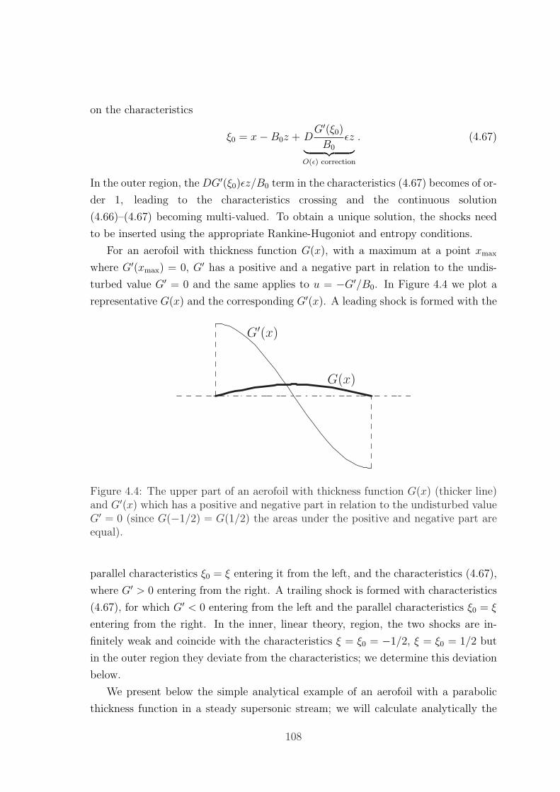
on the characteristics
ξ0 = x−B0z + DG′(ξ0)B0
εz︸ ︷︷ ︸O(ε) correction
. (4.67)
In the outer region, the DG′(ξ0)εz/B0 term in the characteristics (4.67) becomes of or-
der 1, leading to the characteristics crossing and the continuous solution
(4.66)–(4.67) becoming multi-valued. To obtain a unique solution, the shocks need
to be inserted using the appropriate Rankine-Hugoniot and entropy conditions.
For an aerofoil with thickness function G(x), with a maximum at a point xmax
where G′(xmax) = 0, G′ has a positive and a negative part in relation to the undis-
turbed value G′ = 0 and the same applies to u = −G′/B0. In Figure 4.4 we plot a
representative G(x) and the corresponding G′(x). A leading shock is formed with the
G(x)
G′(x)
Figure 4.4: The upper part of an aerofoil with thickness function G(x) (thicker line)and G′(x) which has a positive and negative part in relation to the undisturbed valueG′ = 0 (since G(−1/2) = G(1/2) the areas under the positive and negative part areequal).
parallel characteristics ξ0 = ξ entering it from the left, and the characteristics (4.67),
where G′ > 0 entering from the right. A trailing shock is formed with characteristics
(4.67), for which G′ < 0 entering from the left and the parallel characteristics ξ0 = ξ
entering from the right. In the inner, linear theory, region, the two shocks are in-
finitely weak and coincide with the characteristics ξ = ξ0 = −1/2, ξ = ξ0 = 1/2 but
in the outer region they deviate from the characteristics; we determine this deviation
below.
We present below the simple analytical example of an aerofoil with a parabolic
thickness function in a steady supersonic stream; we will calculate analytically the
108
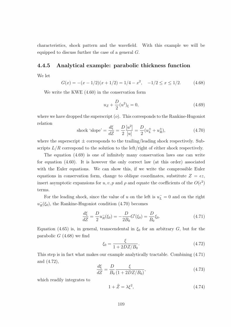
characteristics, shock pattern and the wavefield. With this example we will be
equipped to discuss further the case of a general G.
4.4.5 Analytical example: parabolic thickness function
We let
G(x) = −(x− 1/2)(x+ 1/2) = 1/4− x2, −1/2 ≤ x ≤ 1/2. (4.68)
We write the KWE (4.60) in the conservation form
uZ +D
2(u2)ξ = 0, (4.69)
where we have dropped the superscript (o). This corresponds to the Rankine-Hugoniot
relation
shock ‘slope’ =dξ
dZ=D
2
[u2]
[u]=D
2(u±L + u±R), (4.70)
where the superscript ± corresponds to the trailing/leading shock respectively. Sub-
scripts L/R correspond to the solution to the left/right of either shock respectively.
The equation (4.69) is one of infinitely many conservation laws one can write
for equation (4.60). It is however the only correct law (at this order) associated
with the Euler equations. We can show this, if we write the compressible Euler
equations in conservation form, change to oblique coordinates, substitute Z = εz,
insert asymptotic expansions for u, v, p and ρ and equate the coefficients of the O(ε2)
terms.
For the leading shock, since the value of u on the left is u−L = 0 and on the right
u−R(ξ0), the Rankine-Hugoniot condition (4.70) becomes
dξ
dZ=D
2u−R(ξ0) = − D
2B0
G′(ξ0) =D
B0
ξ0. (4.71)
Equation (4.65) is, in general, transcendental in ξ0 for an arbitrary G, but for the
parabolic G (4.68) we find
ξ0 =ξ
1 + 2DZ/B0
. (4.72)
This step is in fact what makes our example analytically tractable. Combining (4.71)
and (4.72),dξ
dZ=
D
B0
ξ
(1 + 2DZ/B0), (4.73)
which readily integrates to
1 + Z = λξ2, (4.74)
109
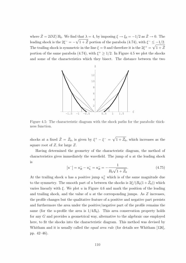
where Z = 2DZ/B0. We find that λ = 4, by imposing ξ → ξ0 = −1/2 as Z → 0. The
leading shock is the 2ξ− = −√
1 + Z portion of the parabola (4.74), with ξ− ≤ −1/2.
The trailing shock is symmetric in the line ξ = 0 and therefore it is the 2ξ+ =√
1 + Z
portion of the same parabola (4.74), with ξ+ ≥ 1/2. In Figure 4.5 we plot the shocks
and some of the characteristics which they bisect. The distance between the two
-1.5 -1 -0.5 0.5 1 1.5Ξ
2
4
6
8
10
12
Z
Figure 4.5: The characteristic diagram with the shock paths for the parabolic thick-ness function.
shocks at a fixed Z = Z0, is given by ξ+ − ξ− =√
1 + Z0, which increases as the
square root of Z, for large Z.
Having determined the geometry of the characteristic diagram, the method of
characteristics gives immediately the wavefield. The jump of u at the leading shock
is
[u−] = u−R − u−L = u−R = − 1
B0
√1 + Z0
. (4.75)
At the trailing shock u has a positive jump u+L which is of the same magnitude due
to the symmetry. The smooth part of u between the shocks is 2ξ/(B0(1 + Z0)) which
varies linearly with ξ. We plot u in Figure 4.6 and mark the position of the leading
and trailing shock, and the value of u at the corresponding jumps. As Z increases,
the profile changes but the qualitative feature of a positive and negative part persists
and furthermore the area under the positive/negative part of the profile remains the
same (for the u-profile the area is 1/4B0). This area conservation property holds
for any G and provides a geometrical way, alternative to the algebraic one employed
here, to fit the shocks into the characteristic diagram. This method was devised by
Whitham and it is usually called the equal area rule (for details see Whitham [126],
pp. 42–46).
110
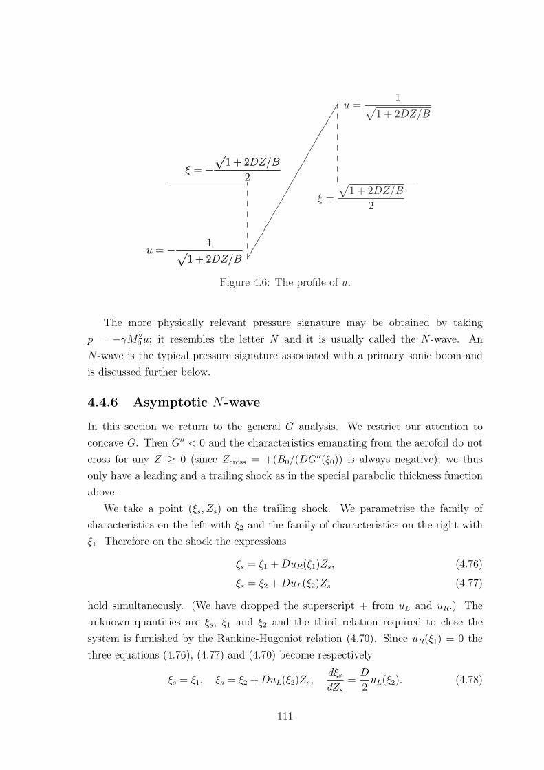
u = − 1√1 + 2DZ/B
ξ = −√
1 + 2DZ/B
2ξ = −
√1 + 2DZ/B
2
u = − 1√1 + 2DZ/B
u =1√
1 + 2DZ/B
ξ =
√1 + 2DZ/B
2
Figure 4.6: The profile of u.
The more physically relevant pressure signature may be obtained by taking
p = −γM20u; it resembles the letter N and it is usually called the N -wave. An
N -wave is the typical pressure signature associated with a primary sonic boom and
is discussed further below.
4.4.6 Asymptotic N-wave
In this section we return to the general G analysis. We restrict our attention to
concave G. Then G′′ < 0 and the characteristics emanating from the aerofoil do not
cross for any Z ≥ 0 (since Zcross = +(B0/(DG′′(ξ0)) is always negative); we thus
only have a leading and a trailing shock as in the special parabolic thickness function
above.
We take a point (ξs, Zs) on the trailing shock. We parametrise the family of
characteristics on the left with ξ2 and the family of characteristics on the right with
ξ1. Therefore on the shock the expressions
ξs = ξ1 +DuR(ξ1)Zs, (4.76)
ξs = ξ2 +DuL(ξ2)Zs (4.77)
hold simultaneously. (We have dropped the superscript + from uL and uR.) The
unknown quantities are ξs, ξ1 and ξ2 and the third relation required to close the
system is furnished by the Rankine-Hugoniot relation (4.70). Since uR(ξ1) = 0 the
three equations (4.76), (4.77) and (4.70) become respectively
ξs = ξ1, ξs = ξ2 +DuL(ξ2)Zs,dξsdZs
=D
2uL(ξ2). (4.78)
111
Ξ1Ξ2
Trailing Shock
Figure 4.7: Schematic that shows the relation between the characteristic labels ξ1 andξ2 mentioned in the text.
We can thus parametrise the shock with the characteristic label ξ2. From the second
relation in (4.78), and dropping the subscript from uL, we have
ξ′s = 1 +Du(ξ2)Z′s +Du′(ξ2)Zs, (4.79)
where the prime denotes differentiation with respect to ξ2. Similarly from the third
(Rankine-Hugoniot) relation in (4.78), we have
ξ′s =D
2u(ξ2)Z
′s. (4.80)
Combining (4.79) and (4.80) in order to eliminate ξ′s, we obtain the first-order ordinary
differential equation
Z ′s + 2u′(ξ2)u(ξ2)
Zs = − 2
Du(ξ2). (4.81)
Integrating this we obtain
1
2(Du(ξ2))
2Zs =
∫ 1/2
ξ2
Du(ξ)dξ (4.82)
⇒Zs(ξ2) =2
Du2(ξ2)
∫ 1/2
ξ2
u(ξ)dξ. (4.83)
Therefore we have determined expressions for ξs(ξ2) and Zs(ξ2) which can be used
to plot the shock very easily for many profile choices.5
5The plotting will be exact in the cases that the integral∫ 1/2
ξ2u(ξ)dξ can be found exactly but
even if this cannot be done it is very simple to calculate the one-dimensional quadrature numerically.
112
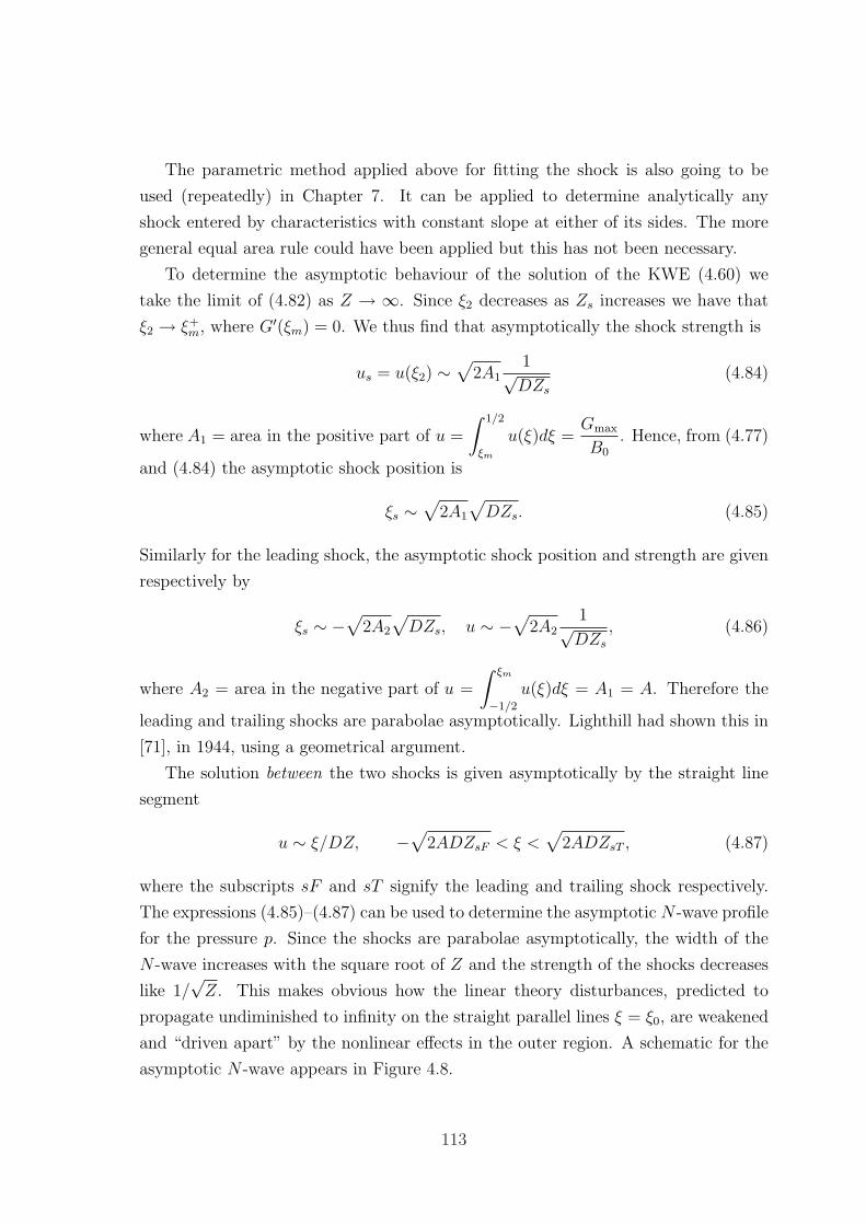
The parametric method applied above for fitting the shock is also going to be
used (repeatedly) in Chapter 7. It can be applied to determine analytically any
shock entered by characteristics with constant slope at either of its sides. The more
general equal area rule could have been applied but this has not been necessary.
To determine the asymptotic behaviour of the solution of the KWE (4.60) we
take the limit of (4.82) as Z → ∞. Since ξ2 decreases as Zs increases we have that
ξ2 → ξ+m, where G′(ξm) = 0. We thus find that asymptotically the shock strength is
us = u(ξ2) ∼√
2A11√DZs
(4.84)
where A1 = area in the positive part of u =
∫ 1/2
ξm
u(ξ)dξ =Gmax
B0
. Hence, from (4.77)
and (4.84) the asymptotic shock position is
ξs ∼√
2A1
√DZs. (4.85)
Similarly for the leading shock, the asymptotic shock position and strength are given
respectively by
ξs ∼ −√
2A2
√DZs, u ∼ −
√2A2
1√DZs
, (4.86)
where A2 = area in the negative part of u =
∫ ξm
−1/2
u(ξ)dξ = A1 = A. Therefore the
leading and trailing shocks are parabolae asymptotically. Lighthill had shown this in
[71], in 1944, using a geometrical argument.
The solution between the two shocks is given asymptotically by the straight line
segment
u ∼ ξ/DZ, −√
2ADZsF < ξ <√
2ADZsT , (4.87)
where the subscripts sF and sT signify the leading and trailing shock respectively.
The expressions (4.85)–(4.87) can be used to determine the asymptotic N -wave profile
for the pressure p. Since the shocks are parabolae asymptotically, the width of the
N -wave increases with the square root of Z and the strength of the shocks decreases
like 1/√Z. This makes obvious how the linear theory disturbances, predicted to
propagate undiminished to infinity on the straight parallel lines ξ = ξ0, are weakened
and “driven apart” by the nonlinear effects in the outer region. A schematic for the
asymptotic N -wave appears in Figure 4.8.
113
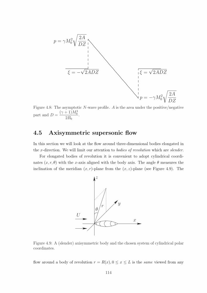
ξ = −√
2ADZ ξ =√
2ADZ
p = −γM 20
√2A
DZ
p = γM 20
√2A
DZ
Figure 4.8: The asymptotic N -wave profile. A is the area under the positive/negative
part and D =(γ + 1)M4
0
2B0
.
4.5 Axisymmetric supersonic flow
In this section we will look at the flow around three-dimensional bodies elongated in
the x-direction. We will limit our attention to bodies of revolution which are slender.
For elongated bodies of revolution it is convenient to adopt cylindrical coordi-
nates (x, r, θ) with the x-axis aligned with the body axis. The angle θ measures the
inclination of the meridian (x, r)-plane from the (x, z)-plane (see Figure 4.9). The
z
y
Uθr
x
Figure 4.9: A (slender) axisymmetric body and the chosen system of cylindrical polarcoordinates.
flow around a body of revolution r = R(x), 0 ≤ x ≤ L is the same viewed from any
114
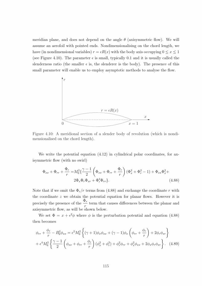
meridian plane, and does not depend on the angle θ (axisymmetric flow). We will
assume an aerofoil with pointed ends. Nondimensionalising on the chord length, we
have (in nondimensional variables) r = εR(x) with the body axis occupying 0 ≤ x ≤ 1
(see Figure 4.10). The parameter ε is small, typically 0.1 and it is usually called the
slenderness ratio (the smaller ε is, the slenderer is the body). The presence of this
small parameter will enable us to employ asymptotic methods to analyse the flow.
0
r = εR(x)
x = 1
x
r
Figure 4.10: A meridional section of a slender body of revolution (which is nondi-mensionalised on the chord length).
We write the potential equation (4.12) in cylindrical polar coordinates, for ax-
isymmetric flow (with no swirl)
Φxx + Φrr +Φr
r=M2
0{γ − 1
2
(Φxx + Φrr +
Φr
r
)(Φ2
x + Φ2r − 1) + ΦxxΦ
2x+
2ΦxΦrΦxr + Φ2rΦrr}. (4.88)
Note that if we omit the Φr/r terms from (4.88) and exchange the coordinate r with
the coordinate z we obtain the potential equation for planar flows. However it is
precisely the presence of theΦr
rterm that causes differences between the planar and
axisymmetric flow, as will be shown below.
We set Φ = x + ε2φ where φ is the perturbation potential and equation (4.88)
then becomes
φrr +φrr−B2
0φxx = ε2M20
{(γ + 1)φxφxx + (γ − 1)φx
(φrr +
φrr
)+ 2φrφxr
}
+ ε4M20
{γ − 1
2
(φxx + φrr +
φrr
)(φ2
x + φ2r) + φ2
rφrr + φ2xφxx + 2φxφrφxr
}. (4.89)
115
The body boundary condition (4.13) should be satisfied. In the current coordinate
system it is expressed as
Φr(x, εR(x))
Φx(x, εR(x))=
ε2φr(x, εR(x))
1 + ε2φx(x, εR(x))= εR′(x). (4.90)
The condition at infinity should be additionally satisfied and we will return to it later.
4.5.1 Asymptotic analysis
¦ Inner region (linear theory)
Linearised slender-body theory is well established and can be found in textbooks
such as Whitham [126], Liepmann and Roshko [70] and Frankl and Karpovich [39].
The minor advantage of our exposition of this theory here is the explicit use of the
small slenderness parameter ε.
Even though, as we have shown, for the two-dimensional problem the linear theory
fails at large distances from the body it is still valuable because it gives the correct
pressure forces acting on the body. Also from Whitham’s point of view, as he explains
in [124], the only failure of the linear theory at first order is that the characteristics
it predicts are incorrect; otherwise the theory predicts correctly the values on the
characteristics and hence the only modification needed to the linear theory is to shift
appropriately the characteristics and introduce shocks in multi-valued regions.
We tentatively assume that the solution of (4.89) is represented by the asymptotic
expansion
φ ∼ φ1 + εαφ2 +O(δ(ε)) where α > 0 and δ(ε) ¿ εα; (4.91)
α is later identified to be equal to 2. We will substitute the expansion (4.91) into
the equation (4.89) and equate the coefficients of terms of same order in ε. (We
emphasise however that the substitution in the boundary condition will be more
subtle.) At leading order we obtain
φ1rr +1
rφ1r −B2
0φ1xx = 0. (4.92)
Under the change x→ t and 1/B20 → c2 we obtain the well-known cylindrical waves
equation
φ1tt − c2(φ1rr +1
rφ1r) = 0,
116
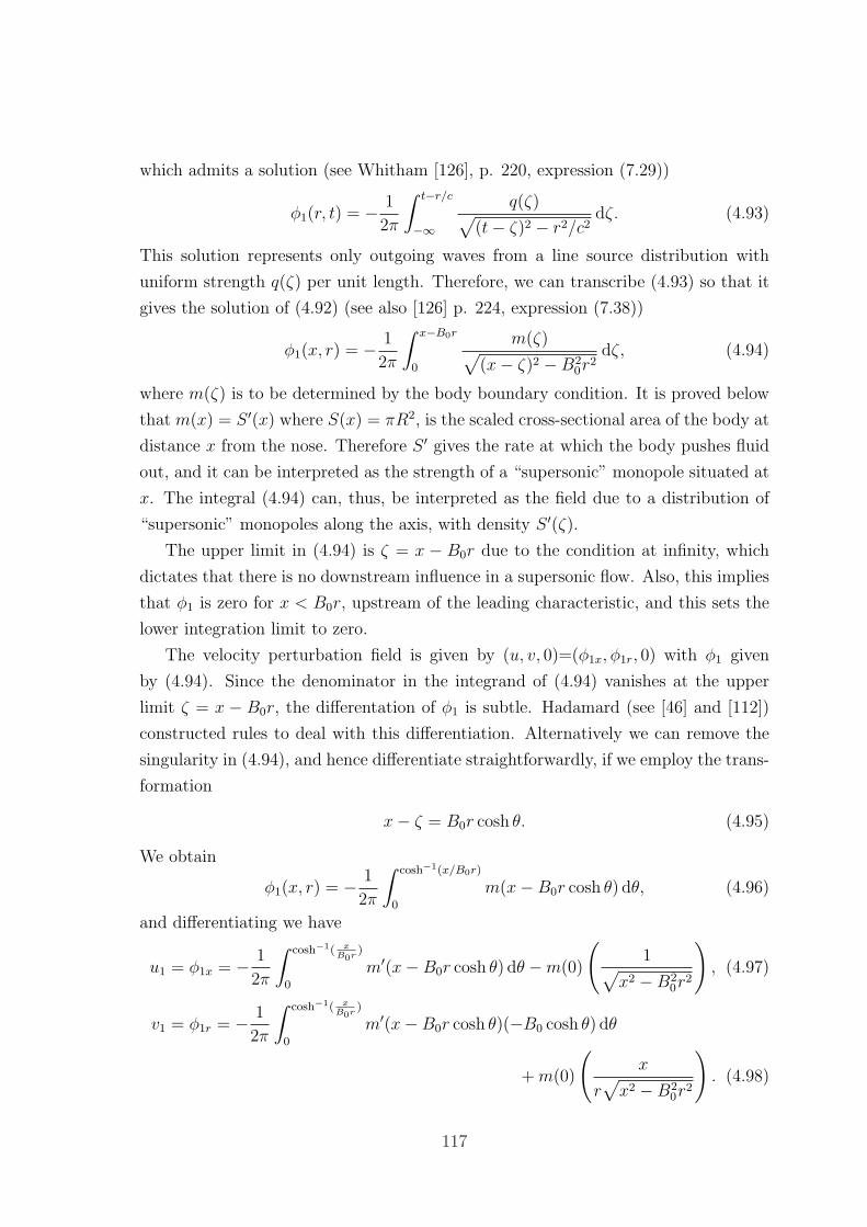
which admits a solution (see Whitham [126], p. 220, expression (7.29))
φ1(r, t) = − 1
2π
∫ t−r/c
−∞
q(ζ)√(t− ζ)2 − r2/c2
dζ. (4.93)
This solution represents only outgoing waves from a line source distribution with
uniform strength q(ζ) per unit length. Therefore, we can transcribe (4.93) so that it
gives the solution of (4.92) (see also [126] p. 224, expression (7.38))
φ1(x, r) = − 1
2π
∫ x−B0r
0
m(ζ)√(x− ζ)2 −B2
0r2
dζ, (4.94)
where m(ζ) is to be determined by the body boundary condition. It is proved below
that m(x) = S ′(x) where S(x) = πR2, is the scaled cross-sectional area of the body at
distance x from the nose. Therefore S ′ gives the rate at which the body pushes fluid
out, and it can be interpreted as the strength of a “supersonic” monopole situated at
x. The integral (4.94) can, thus, be interpreted as the field due to a distribution of
“supersonic” monopoles along the axis, with density S ′(ζ).
The upper limit in (4.94) is ζ = x − B0r due to the condition at infinity, which
dictates that there is no downstream influence in a supersonic flow. Also, this implies
that φ1 is zero for x < B0r, upstream of the leading characteristic, and this sets the
lower integration limit to zero.
The velocity perturbation field is given by (u, v, 0)=(φ1x, φ1r, 0) with φ1 given
by (4.94). Since the denominator in the integrand of (4.94) vanishes at the upper
limit ζ = x − B0r, the differentation of φ1 is subtle. Hadamard (see [46] and [112])
constructed rules to deal with this differentiation. Alternatively we can remove the
singularity in (4.94), and hence differentiate straightforwardly, if we employ the trans-
formation
x− ζ = B0r cosh θ. (4.95)
We obtain
φ1(x, r) = − 1
2π
∫ cosh−1(x/B0r)
0
m(x−B0r cosh θ) dθ, (4.96)
and differentiating we have
u1 = φ1x = − 1
2π
∫ cosh−1( xB0r
)
0
m′(x−B0r cosh θ) dθ −m(0)
(1√
x2 −B20r
2
), (4.97)
v1 = φ1r = − 1
2π
∫ cosh−1( xB0r
)
0
m′(x−B0r cosh θ)(−B0 cosh θ) dθ
+m(0)
(x
r√x2 −B2
0r2
). (4.98)
117
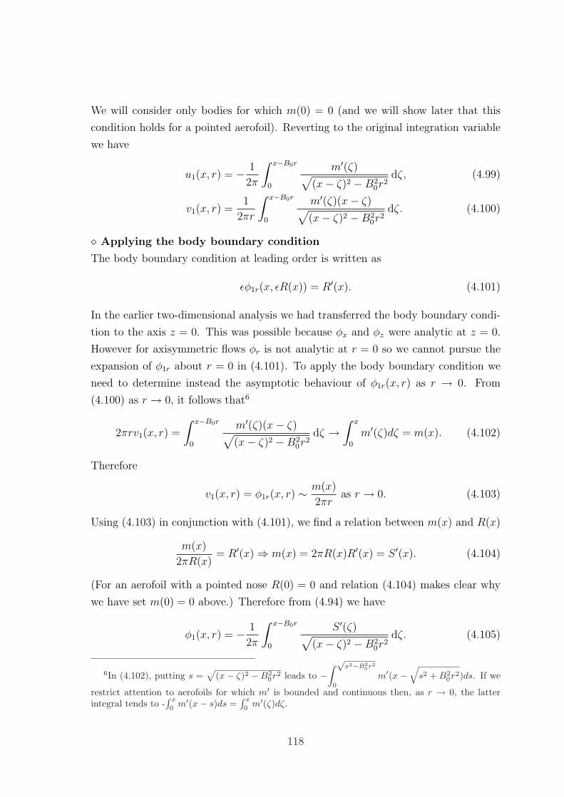
We will consider only bodies for which m(0) = 0 (and we will show later that this
condition holds for a pointed aerofoil). Reverting to the original integration variable
we have
u1(x, r) = − 1
2π
∫ x−B0r
0
m′(ζ)√(x− ζ)2 −B2
0r2
dζ, (4.99)
v1(x, r) =1
2πr
∫ x−B0r
0
m′(ζ)(x− ζ)√(x− ζ)2 −B2
0r2
dζ. (4.100)
¦ Applying the body boundary condition
The body boundary condition at leading order is written as
εφ1r(x, εR(x)) = R′(x). (4.101)
In the earlier two-dimensional analysis we had transferred the body boundary condi-
tion to the axis z = 0. This was possible because φx and φz were analytic at z = 0.
However for axisymmetric flows φr is not analytic at r = 0 so we cannot pursue the
expansion of φ1r about r = 0 in (4.101). To apply the body boundary condition we
need to determine instead the asymptotic behaviour of φ1r(x, r) as r → 0. From
(4.100) as r → 0, it follows that6
2πrv1(x, r) =
∫ x−B0r
0
m′(ζ)(x− ζ)√(x− ζ)2 −B2
0r2
dζ →∫ x
0
m′(ζ)dζ = m(x). (4.102)
Therefore
v1(x, r) = φ1r(x, r) ∼ m(x)
2πras r → 0. (4.103)
Using (4.103) in conjunction with (4.101), we find a relation between m(x) and R(x)
m(x)
2πR(x)= R′(x) ⇒ m(x) = 2πR(x)R′(x) = S ′(x). (4.104)
(For an aerofoil with a pointed nose R(0) = 0 and relation (4.104) makes clear why
we have set m(0) = 0 above.) Therefore from (4.94) we have
φ1(x, r) = − 1
2π
∫ x−B0r
0
S ′(ζ)√(x− ζ)2 −B2
0r2
dζ. (4.105)
6In (4.102), putting s =√
(x− ζ)2 −B20r2 leads to −
∫ √x2−B2
0r2
0
m′(x−√
s2 + B20r2)ds. If we
restrict attention to aerofoils for which m′ is bounded and continuous then, as r → 0, the latterintegral tends to -
∫ x
0m′(x− s)ds =
∫ x
0m′(ζ)dζ.
118
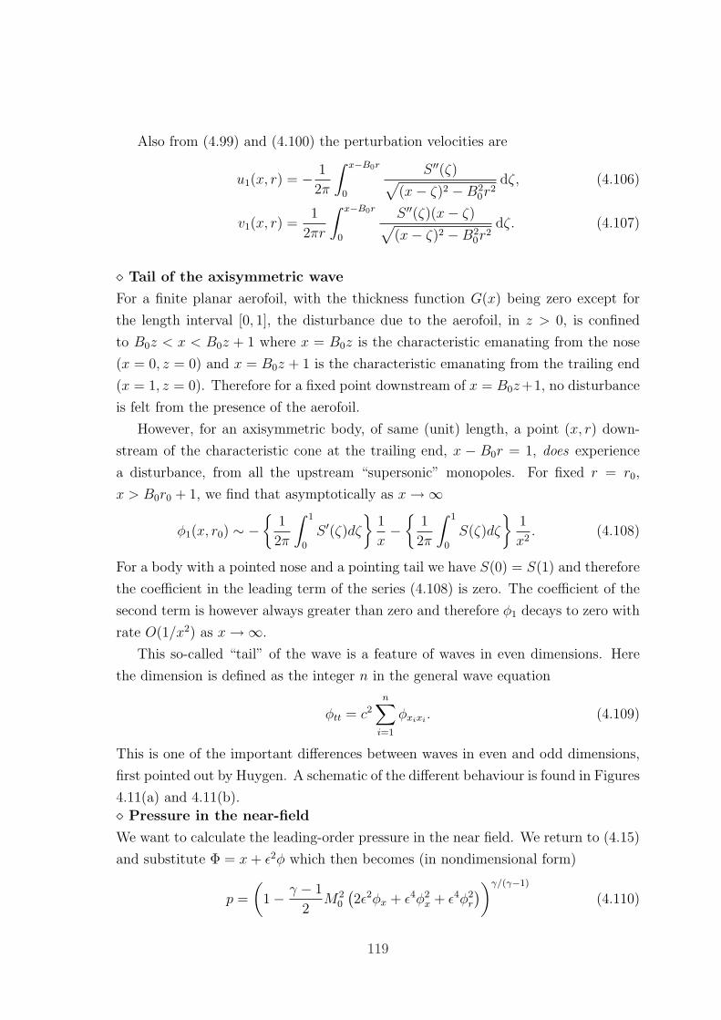
Also from (4.99) and (4.100) the perturbation velocities are
u1(x, r) = − 1
2π
∫ x−B0r
0
S ′′(ζ)√(x− ζ)2 −B2
0r2
dζ, (4.106)
v1(x, r) =1
2πr
∫ x−B0r
0
S ′′(ζ)(x− ζ)√(x− ζ)2 −B2
0r2
dζ. (4.107)
¦ Tail of the axisymmetric wave
For a finite planar aerofoil, with the thickness function G(x) being zero except for
the length interval [0, 1], the disturbance due to the aerofoil, in z > 0, is confined
to B0z < x < B0z + 1 where x = B0z is the characteristic emanating from the nose
(x = 0, z = 0) and x = B0z + 1 is the characteristic emanating from the trailing end
(x = 1, z = 0). Therefore for a fixed point downstream of x = B0z+1, no disturbance
is felt from the presence of the aerofoil.
However, for an axisymmetric body, of same (unit) length, a point (x, r) down-
stream of the characteristic cone at the trailing end, x − B0r = 1, does experience
a disturbance, from all the upstream “supersonic” monopoles. For fixed r = r0,
x > B0r0 + 1, we find that asymptotically as x→∞
φ1(x, r0) ∼ −{
1
2π
∫ 1
0
S ′(ζ)dζ}
1
x−
{1
2π
∫ 1
0
S(ζ)dζ
}1
x2. (4.108)
For a body with a pointed nose and a pointing tail we have S(0) = S(1) and therefore
the coefficient in the leading term of the series (4.108) is zero. The coefficient of the
second term is however always greater than zero and therefore φ1 decays to zero with
rate O(1/x2) as x→∞.
This so-called “tail” of the wave is a feature of waves in even dimensions. Here
the dimension is defined as the integer n in the general wave equation
φtt = c2n∑i=1
φxixi. (4.109)
This is one of the important differences between waves in even and odd dimensions,
first pointed out by Huygen. A schematic of the different behaviour is found in Figures
4.11(a) and 4.11(b).
¦ Pressure in the near-field
We want to calculate the leading-order pressure in the near field. We return to (4.15)
and substitute Φ = x+ ε2φ which then becomes (in nondimensional form)
p =
(1− γ − 1
2M2
0
(2ε2φx + ε4φ2
x + ε4φ2r
))γ/(γ−1)
(4.110)
119
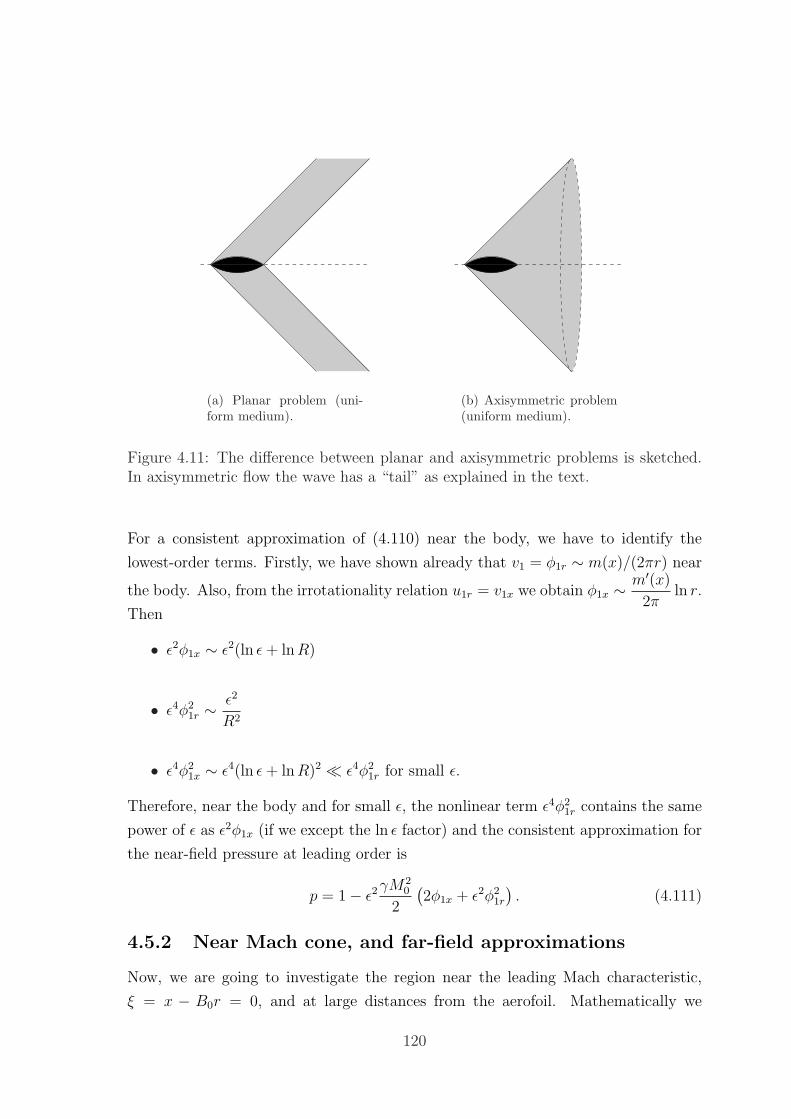
(a) Planar problem (uni-form medium).
(b) Axisymmetric problem(uniform medium).
Figure 4.11: The difference between planar and axisymmetric problems is sketched.In axisymmetric flow the wave has a “tail” as explained in the text.
For a consistent approximation of (4.110) near the body, we have to identify the
lowest-order terms. Firstly, we have shown already that v1 = φ1r ∼ m(x)/(2πr) near
the body. Also, from the irrotationality relation u1r = v1x we obtain φ1x ∼ m′(x)2π
ln r.
Then
• ε2φ1x ∼ ε2(ln ε+ lnR)
• ε4φ21r ∼
ε2
R2
• ε4φ21x ∼ ε4(ln ε+ lnR)2 ¿ ε4φ2
1r for small ε.
Therefore, near the body and for small ε, the nonlinear term ε4φ21r contains the same
power of ε as ε2φ1x (if we except the ln ε factor) and the consistent approximation for
the near-field pressure at leading order is
p = 1− ε2γM2
0
2
(2φ1x + ε2φ2
1r
). (4.111)
4.5.2 Near Mach cone, and far-field approximations
Now, we are going to investigate the region near the leading Mach characteristic,
ξ = x − B0r = 0, and at large distances from the aerofoil. Mathematically we
120
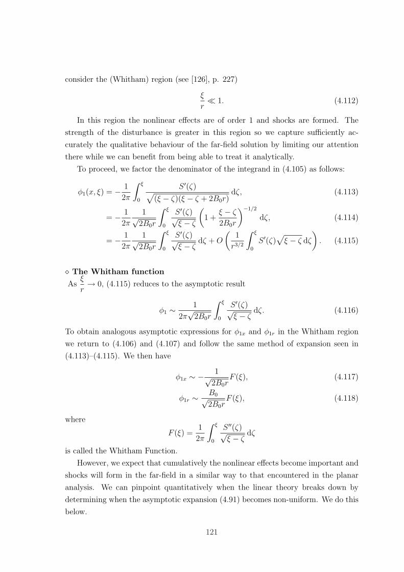
consider the (Whitham) region (see [126], p. 227)
ξ
r¿ 1. (4.112)
In this region the nonlinear effects are of order 1 and shocks are formed. The
strength of the disturbance is greater in this region so we capture sufficiently ac-
curately the qualitative behaviour of the far-field solution by limiting our attention
there while we can benefit from being able to treat it analytically.
To proceed, we factor the denominator of the integrand in (4.105) as follows:
φ1(x, ξ) = − 1
2π
∫ ξ
0
S ′(ζ)√(ξ − ζ)(ξ − ζ + 2B0r)
dζ, (4.113)
= − 1
2π
1√2B0r
∫ ξ
0
S ′(ζ)√ξ − ζ
(1 +
ξ − ζ
2B0r
)−1/2
dζ, (4.114)
= − 1
2π
1√2B0r
∫ ξ
0
S ′(ζ)√ξ − ζ
dζ +O
(1
r3/2
∫ ξ
0
S ′(ζ)√ξ − ζ dζ
). (4.115)
¦ The Whitham function
Asξ
r→ 0, (4.115) reduces to the asymptotic result
φ1 ∼ 1
2π√
2B0r
∫ ξ
0
S ′(ζ)√ξ − ζ
dζ. (4.116)
To obtain analogous asymptotic expressions for φ1x and φ1r in the Whitham region
we return to (4.106) and (4.107) and follow the same method of expansion seen in
(4.113)–(4.115). We then have
φ1x ∼ − 1√2B0r
F (ξ), (4.117)
φ1r ∼ B0√2B0r
F (ξ), (4.118)
where
F (ξ) =1
2π
∫ ξ
0
S ′′(ζ)√ξ − ζ
dζ
is called the Whitham Function.
However, we expect that cumulatively the nonlinear effects become important and
shocks will form in the far-field in a similar way to that encountered in the planar
analysis. We can pinpoint quantitatively when the linear theory breaks down by
determining when the asymptotic expansion (4.91) becomes non-uniform. We do this
below.
121
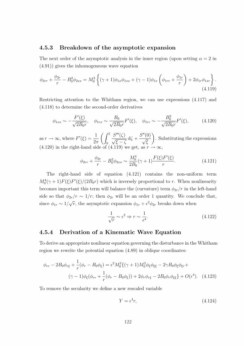
4.5.3 Breakdown of the asymptotic expansion
The next order of the asymptotic analysis in the inner region (upon setting α = 2 in
(4.91)) gives the inhomogeneous wave equation
φ2rr +φ2r
r−B2
0φ2xx = M20
{(γ + 1)φ1xφ1xx + (γ − 1)φ1x
(φ1rr +
φ1r
r
)+ 2φ1rφ1xr
}.
(4.119)
Restricting attention to the Whitham region, we can use expressions (4.117) and
(4.118) to determine the second-order derivatives
φ1xx ∼ − F ′(ξ)√2B0r
, φ1rx ∼ B0√2B0r
F ′(ξ), φ1rr ∼ − B20√
2B0rF ′(ξ), (4.120)
as r →∞, where F ′(ξ) =1
2π
(∫ ξ
0
S ′′′(ζ)√ξ − ζ
dζ +S ′′(0)√
ξ
). Substituting the expressions
(4.120) in the right-hand side of (4.119) we get, as r →∞,
φ2rr +φ2r
r−B2
0φ2xx ∼ M40
2B0
(γ + 1)F (ξ)F ′(ξ)
r. (4.121)
The right-hand side of equation (4.121) contains the non-uniform term
M40 (γ + 1)F (ξ)F ′(ξ)/(2B0r) which is inversely proportional to r. When nonlinearity
becomes important this term will balance the (curvature) term φ2r/r in the left-hand
side so that φ2r/r ∼ 1/r; then φ2r will be an order 1 quantity. We conclude that,
since φ1r ∼ 1/√r, the asymptotic expansion φ1r + ε2φ2r breaks down when
1√r∼ ε2 ⇒ r ∼ 1
ε4. (4.122)
4.5.4 Derivation of a Kinematic Wave Equation
To derive an appropriate nonlinear equation governing the disturbance in the Whitham
region we rewrite the potential equation (4.89) in oblique coordinates:
φrr − 2B0φrξ +1
r(φr −B0φξ) = ε2M2
0{(γ + 1)M20φξφξξ − 2γB0φξφξr+
(γ − 1)φξ(φrr +1
r(φr −B0φξ)) + 2φrφrξ − 2B0φrφξξ}+O(ε4). (4.123)
To remove the secularity we define a new rescaled variable
Y = ε4r, (4.124)
122
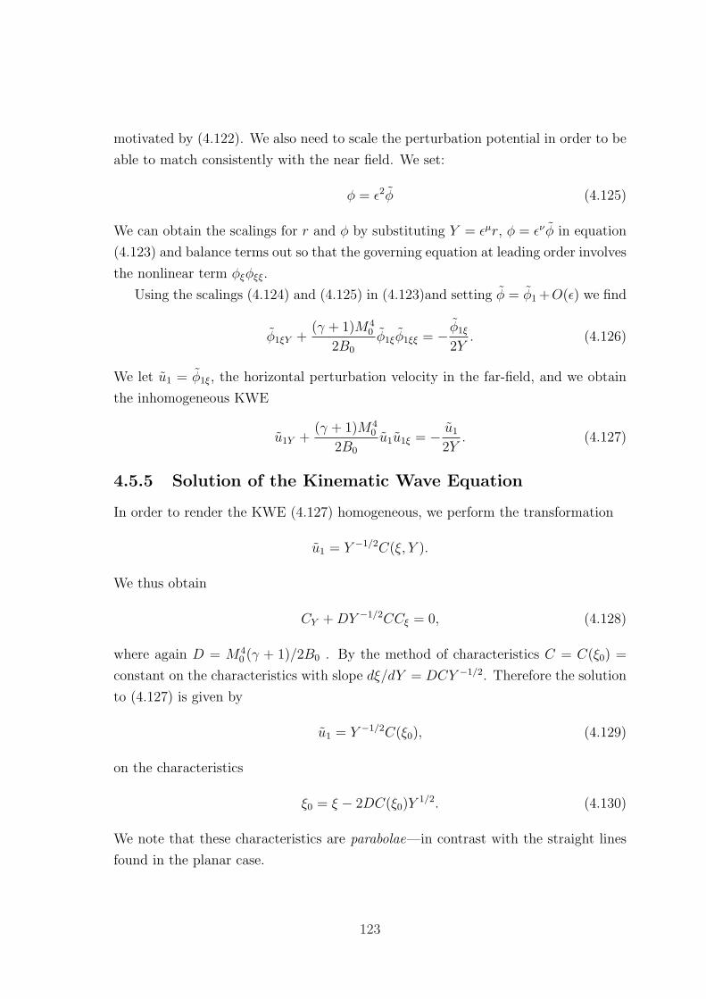
motivated by (4.122). We also need to scale the perturbation potential in order to be
able to match consistently with the near field. We set:
φ = ε2φ (4.125)
We can obtain the scalings for r and φ by substituting Y = εµr, φ = ενφ in equation
(4.123) and balance terms out so that the governing equation at leading order involves
the nonlinear term φξφξξ.
Using the scalings (4.124) and (4.125) in (4.123)and setting φ = φ1 +O(ε) we find
φ1ξY +(γ + 1)M4
0
2B0
φ1ξφ1ξξ = − φ1ξ
2Y. (4.126)
We let u1 = φ1ξ, the horizontal perturbation velocity in the far-field, and we obtain
the inhomogeneous KWE
u1Y +(γ + 1)M4
0
2B0
u1u1ξ = − u1
2Y. (4.127)
4.5.5 Solution of the Kinematic Wave Equation
In order to render the KWE (4.127) homogeneous, we perform the transformation
u1 = Y −1/2C(ξ, Y ).
We thus obtain
CY +DY −1/2CCξ = 0, (4.128)
where again D = M40 (γ + 1)/2B0 . By the method of characteristics C = C(ξ0) =
constant on the characteristics with slope dξ/dY = DCY −1/2. Therefore the solution
to (4.127) is given by
u1 = Y −1/2C(ξ0), (4.129)
on the characteristics
ξ0 = ξ − 2DC(ξ0)Y1/2. (4.130)
We note that these characteristics are parabolae—in contrast with the straight lines
found in the planar case.
123
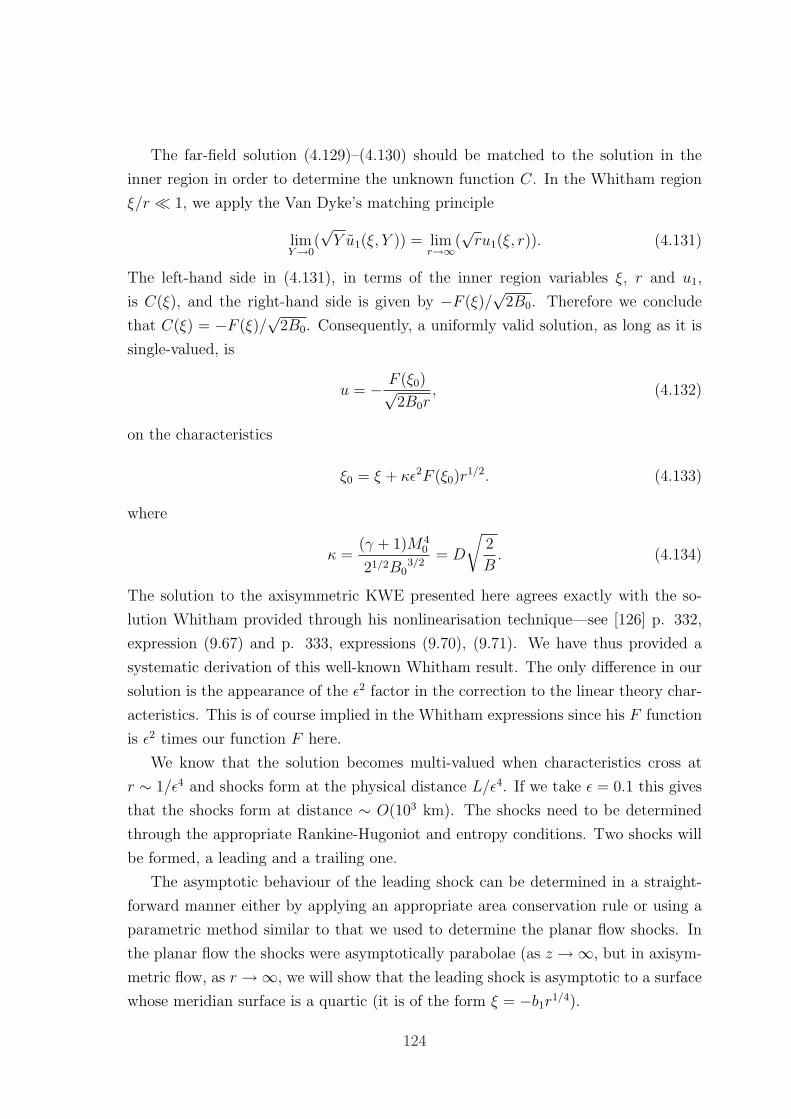
The far-field solution (4.129)–(4.130) should be matched to the solution in the
inner region in order to determine the unknown function C. In the Whitham region
ξ/r ¿ 1, we apply the Van Dyke’s matching principle
limY→0
(√Y u1(ξ, Y )) = lim
r→∞(√ru1(ξ, r)). (4.131)
The left-hand side in (4.131), in terms of the inner region variables ξ, r and u1,
is C(ξ), and the right-hand side is given by −F (ξ)/√
2B0. Therefore we conclude
that C(ξ) = −F (ξ)/√
2B0. Consequently, a uniformly valid solution, as long as it is
single-valued, is
u = − F (ξ0)√2B0r
, (4.132)
on the characteristics
ξ0 = ξ + κε2F (ξ0)r1/2. (4.133)
where
κ =(γ + 1)M4
0
21/2B03/2
= D
√2
B. (4.134)
The solution to the axisymmetric KWE presented here agrees exactly with the so-
lution Whitham provided through his nonlinearisation technique—see [126] p. 332,
expression (9.67) and p. 333, expressions (9.70), (9.71). We have thus provided a
systematic derivation of this well-known Whitham result. The only difference in our
solution is the appearance of the ε2 factor in the correction to the linear theory char-
acteristics. This is of course implied in the Whitham expressions since his F function
is ε2 times our function F here.
We know that the solution becomes multi-valued when characteristics cross at
r ∼ 1/ε4 and shocks form at the physical distance L/ε4. If we take ε = 0.1 this gives
that the shocks form at distance ∼ O(103 km). The shocks need to be determined
through the appropriate Rankine-Hugoniot and entropy conditions. Two shocks will
be formed, a leading and a trailing one.
The asymptotic behaviour of the leading shock can be determined in a straight-
forward manner either by applying an appropriate area conservation rule or using a
parametric method similar to that we used to determine the planar flow shocks. In
the planar flow the shocks were asymptotically parabolae (as z →∞, but in axisym-
metric flow, as r →∞, we will show that the leading shock is asymptotic to a surface
whose meridian surface is a quartic (it is of the form ξ = −b1r1/4).
124
We first consider a point (ξs, Ys) on the leading shock. We parametrise the family
of characteristics on the left of the shock with ξ1 and the family of characteristics on
the right with ξ2 in a similar way to that in the planar flow analysis for the trailing
shock. Therefore on the shock the expressions
ξs = ξ1 + 2DC(ξ1)Y1/2s , (4.135)
ξs = ξ2 + 2DC(ξ2)Y1/2s (4.136)
hold simultaneously. The unknown quantities are ξs, ξ1 and ξ2 and the third relation
required to close the system is furnished by the Rankine-Hugoniot relation
dξsdYs
=D
2(C(ξ1) + C(ξ2))Y
−1/2s . (4.137)
Ahead of the leading shock the disturbance is zero and therefore C(ξ1) = 0. Hence
the three equations (4.135), (4.136) and (4.137) become respectively
ξs = ξ1, ξs = ξ2 + 2DC(ξ2)Y1/2s ,
dξsdYs
=D
2C(ξ2)Y
−1/2s . (4.138)
We will parametrise the shock with the characteristic label ξ2. From the second
relation in (4.138) we have
ξ′s = 1 +DC(ξ2)Y−1/2s Y ′
s + 2DC ′(ξ2)Y 1/2s , (4.139)
where the prime denotes differentiation with respect to ξ2. Similarly from the third
(Rankine-Hugoniot) relation in (4.138), we have
ξ′s =D
2C(ξ2)Y
−1/2s Y ′
s . (4.140)
Combining (4.139) and (4.140) in order to eliminate ξ′s, we obtain the first-order
nonlinear ordinary differential equation
Y ′s + 4
C ′(ξ2)C(ξ2)
Ys = − 2Y1/2s
DC(ξ2). (4.141)
We now use the transformation w = Y1/2s in (4.141) and obtain
w′ + 2C ′(ξ2)C(ξ2)
w = − 1
DC(ξ2). (4.142)
This is precisely the same equation as (4.81) which we had integrated and obtained
(4.82). Therefore we have
C(ξ2)2Y 1/2
s = − 1
D
∫ ξ2
0
C(ξ′)dξ′, (4.143)
125
Therefore, since C = −F/√2B0 we get
F (ξ2) ∼(
2
κ
∫ ξ2
0
F (ξ′)dξ′)1/2
Y −1/4s (4.144)
where κ is defined in (4.134). Hence, asymptotically the shock position is given by
ξs ∼ ξ2 −(
2κ
∫ ξ2
0
F (ξ′)dξ′)1/2
Y 1/4s , (4.145)
= ξ2 −(
2κ
∫ ξ2
0
F (ξ′)dξ′)1/2
εr1/4s , (4.146)
which agrees with the Whitham expression in [126], p. 335, expression (9.77), apart
from the ε factor, bearing in mind that Whitham’s F is ε2 ours. Consequently, using
(4.129) and (4.144), we find that the jump of u on the shock is given by
[us] ∼ − 1√2B0
(2
κ
∫ ξ2
0
F (ξ′)dξ′)1/2
Y −3/4s . (4.147)
The fact that for flow around bodies of revolution the width of the N -wave varies as
r1/4 and the shock strength as r−3/4 was first noted by DuMond et al. in [35]. Using
the relation p = −γM20 u we can express (4.147) in terms of the pressure jump across
the shock, [ps]. We find
[ps] ∼ γM20√
2B0
(2
κ
∫ ξ2
0
F (ξ′)dξ′)1/2
Y −3/4s . (4.148)
Using (4.134) in (4.148) along with Ys = ε4r and [ps] = ε−2[ps] (so that we write the
expression in terms of original variables—see (4.125)) we find
[ps] ∼ 21/4γ
(γ + 1)1/2(M2
0 − 1)1/8
(∫ ξ2
0
F (ξ′)dξ′)1/2
ε−1r−3/4. (4.149)
In the physical variables the pressure is p = p0(1 + ε2ps) and therefore its jump is
[p
p0
]= ε2[ps] ∼ 21/4γ
(γ + 1)1/2(M2
0 − 1)1/8
(∫ ξ2
0
F (ξ′)dξ′)1/2
εr−3/4, (4.150)
which agrees with Whitham [126], p. 336, expression (9.78). The latter formula
shows that the strength of a primary boom has a very weak dependence on the Mach
number M0 and decreases with distance like r−3/4. Information about the geometry
of the aerofoil is encompassed in the term
(∫ ξ2
0
F (ξ′)dξ′)1/2
.
126
We have thus derived asymptotic expressions for the leading shock position and
strength. Determining the trailing shock surface is more complicated due to the tail
of the wave. This is also of the form ξ = b2r1/4 and details are found in Whitham’s
paper [124]. The asymptotic form of the wave is an N -wave as in the planar analysis
except that here the disturbance downstream of the trailing shock is non-zero, due to
the presence of the tail.
127
Chapter 5
Two-dimensional steady supersonicmotion in a stratified medium withwind
This chapter extends the work of Chapter 4 to show how small nonlinear and strat-
ification effects become cumulatively important in the far-field for the scenario of
a steadily moving supersonic aerofoil in a weakly stratified atmosphere and with a
weakly stratified wind. This scenario constitutes a paradigm problem for secondary
sonic boom.
5.1 Introduction
In this chapter we investigate two-dimensional flow around a thin supersonic aerofoil
of chord length L, moving at constant speed U , along the x-axis, from right to left,
in a medium weakly stratified in the z-direction, with a horizontal weakly stratified
wind. As in the previous chapter the aerofoil velocity is (−U, 0) but now the ambient
pressure p0(z), density ρ0(z) and temperature T0(z) are all varying. The altitude of
flight, z = 0, will be taken to be the reference level, and the pressure and density
values there are denoted by P0 and D0 respectively. We will represent the wind with
w0(z) = (w0(z), 0), and therefore the air-speed of the aerofoil is U0 = U +w0(0). The
Mach number of the aerofoil is then M0 = U0/c0 = U0
√D0/(γP0), and we assume
that M0 > 1.
As in the previous chapter, we take the aerofoil to be symmetric with respect to
its axis of motion, and with a thickness function G, and we denote by ε again the
thickness ratio Gmax/L; this is typically of order 10−1. A thin aerofoil induces weak
perturbations to the ambient medium and all shocks are weak. We have shown that
128
for a uniform medium the strength of the shocks is of order ε. In a stratified medium
the order of the perturbations may change but it will still involve a positive power of
ε. The ambient properties vary on the scale height of the atmosphere H = P0/(D0g),
already introduced in Chapter 3; for a typical atmosphere H is around 8 km. There-
fore we can identify a second small parameter δ = L/H which is of order 10−3, as we
did in Chapter 3; however here we will address the stratification effects more fully.
The presence of the small parameters ε and δ points to the use of asymptotic
methods. Abandoning the assumption of potential flow we will seek consistent ap-
proximations to the Euler equations, in various regions of interest. For typical atmo-
spheric conditions it is reasonable to proceed with the assumption δ ¿ ε2. We will
employ the method of Matched Asymptotic Expansions to show that
• Near the aerofoil nonlinear and stratification effects are negligible to leading
order and the Euler equations are approximated by a linear wave equation with
constant coefficients as that of the previous chapter. This region will be the
inner region (or near-field).
• At distanceL
εfrom the aerofoil (about 10 aerofoil lengths away), nonlinear
effects become of order 1 but stratification effects are still negligible. We will call
this the middle region (or mid-field). The Euler equations will be approximated
by a KWE which is the same as the KWE in the far-field in the previous chapter.
• Further out stratification effects also become of order 1, at distanceL
δÀ L
ε2À L
ε(about 1000 aerofoil lengths away). We will call this region the outer region (or
far-field). A more complicated KWE then arises.
Our work is related to work by Helfand [55] and Pechuzal and Kevorkian [91]. Helfand
studied the simpler scenario of a thin aerofoil in a stationary atmosphere with a weakly
stratified temperature profile and Pechuzal and Kevorkian studied the scenario of a
thin aerofoil in a uniform atmosphere with a weakly linearly stratified wind. Both
these studies employed the method of Multiple Scales and the stratification parameter
δ was assumed to be of order ε.
5.2 The Euler equations and nondimensionalisa-
tion
Since the motion is steady we again adopt the aerodynamic frame of reference, in
which the aerofoil is stationary and with the stream (U + w0(z), 0) incident on it.
129
Therefore the Euler equations (2.4), (2.4), (2.14), upon switching to the travelling
coordinate X = x+ Ut become
(ρu)X + (ρv)z = 0, (5.1)
pX + ρuuX + ρvuz = 0, (5.2)
pz + ρuvX + ρvvz = −ρg, (5.3)
ρ(upX + vpz) = γp(uρX + vρz). (5.4)
We note that in contrast with Chapter 3, we will retain the term −ρg in the momen-
tum equation and will show consistently that internal gravity waves are not excited
at the order we will be working to. (In Chapter 3, we had neglected this term because
for secondary sonic boom propagation acoustic waves are decoupled from the gravity
waves.) We further note that the naming of the dependent variables is somewhat
unconventional in that we take v to be the velocity in the z-direction, and w0 to be
the wind in the x-direction. Also, from now on, for notational convenience, we will
denote X by x.
We nondimensionalise the system (5.1)–(5.4) using x = x/L, z = z/L and
u = U0(u0(δz) + εu), v = εU0v, p = P0(p0(δz) + εp), ρ = D0(ρ0(δz) + ερ). (5.5)
In expression (5.5) we have defined
u0(δz) =U + w0(z)
U0
, (5.6)
so that u0(0) = 1, and similarly p0(0) = 1 and ρ0(0) = 1. Dropping the hats and
defining, for convenience, a new variable z = δz, we find the nondimensional equations
ε(u0ρx + ρ0ux + ρ0vz) + ε2((ρu)x + (ρv)z) + εδρ0zv = 0, (5.7)
ε(px + γM20ρ0u0ux) + γM2
0 ε2(ρ0uux + u0ρux + ρ0vuz)+
γM20 ε
3(ρuux + ρvuz) + γM20 εδρ0u0zv + γM2
0 ε2δu0zρv = 0,
(5.8)
ε(pz + γM20ρ0u0vx) + γM2
0 ε2(ρ0uvx + u0ρvx + ρ0vvz) + γM2
0 ε3(ρuvx + ρvvz)
= −δ(p0z + ρ0)− εδρ,(5.9)
ε(ρ0u0px) + ε2(ρ0upx + ρ0vpz + u0ρpx) + ε3(ρupx + ρvpz) + εδρ0p0zv + ε2δp0zρv =
γε(p0u0ρx) + γε2(p0uρx + p0vρz + u0pρx) + γε3(puρx + pvρz) + γεδp0ρ0zv + γε2δρ0zpv.(5.10)
In equation (5.9) the first term on the right-hand side, −δ(p0z + ρ0), is zero because
of the hydrostatic balance relation p0z = −ρ0. Note that in the nondimensionalised
system above we have presented the terms in ascending order in the powers of ε.
130
5.2.1 Inner region (near-field)
When we substitute the Taylor series
ρ0(δz) = ρ0(0) + δzρ0z(0) +O(δ2), (5.11)
p0(δz) = p0(0) + δzp0z(0) +O(δ2), (5.12)
u0(δz) = u0(0) + δzu0z(0) +O(δ2), (5.13)
into (5.7)–(5.10), we find that the lowest-order stratification terms involve εδz. Since
we are going to deal with terms only of order ε and order ε2 these stratification terms
are negligible.
Next, we assume that the perturbations can be represented by the asymptotic
series
ρ(x, z) ∼ ρ1 + ερ2 +O(ε2), (5.14)
p(x, z) ∼ p1 + εp2 +O(ε2), (5.15)
u(x, z) ∼ u1 + εu2 +O(ε2), (5.16)
v(x, z) ∼ v1 + εv2 +O(ε2). (5.17)
We substitute (5.14)–(5.17) into (5.7)–(5.10) and we obtain at order ε the linear
system
ρ1x + u1x + v1z = 0, (5.18)
p1x + γM20u1x = 0, (5.19)
p1z + γM20 v1x = 0, (5.20)
p1x − γρ1x = 0. (5.21)
Eliminating p1 and ρ1 from (5.18)–(5.21) we obtain the following linear wave
equation for u1:
u1zz −B20u1xx = 0. (5.22)
Equation (5.22) is the consistent leading-order approximation of the Euler equations
in the near-field. Note that
v1x − u1z = 0 (5.23)
holds, and therefore the vorticity at this order is zero. (This is obtained by integrating
(5.19) with respect to x, differentating with respect to z, and using the resulting
131

relation in (5.20) to eliminate p1z. All integration constants are set to zero due to
the upstream conditions.) The characteristics of equation (5.22) are the straight lines
ξ = x − B0z, η = x + B0z and the D’Alembert solution is φ1(ξ, η) = f(ξ) + g(η).
Concentrating on the half-plane z > 0 the flow quantities at order ε are
u1 = −G′(ξ)B0
, v1 = −B0u1(ξ), p1 = −γM20u1(ξ), ρ1 = −M2
0u1(ξ), (5.24)
just as in (4.31), (4.34) and (4.35) from Chapter 4. Then, proceeding to order ε2 we
find:
ρ2x + u2x + v2z = −ρ1(u1x + v1z)− (u1ρ1x + v1ρ1z), (5.25)
p2x + γM20u2x = −γM2
0 (u1u1x + v1u1z + ρ1u1x), (5.26)
p2z + γM20 v2x = −γM2
0 (u1v1x + v1v1z + ρ1v1x), (5.27)
p2x − γρ2x = −ρ1p1x + γp1ρ1x + (γu1ρ1x − u1p1x) + (γv1ρ1z − v1p1z). (5.28)
The left-hand side at order ε2 is the same as that of the order ε system, upon changing
the subscript ′′1′′ to ′′2′′ (as expected). We use the order ε solution (5.24) to evaluate
the right-hand sides of the system (5.25)–(5.28) in terms of u1 and subsequently use
u1 = −G′(ξ)B0
. We obtain
ρ2x + u2x + v2z = 2M40u1u1ξ = 2
M40
B20
G′G′′, (5.29)
p2x + γM20u2x = 0, (5.30)
p2z + γM20 v2x = 0, (5.31)
p2x − γρ2x = γ(γ − 1)M40u1u1ξ = γ(γ − 1)
M40
B20
G′G′′, (5.32)
where the dash signifies differentation with respect to ξ. Integrating (5.30) with
respect to x we obtain p2 = −γM20u2(x, z) + f(z). The undetermined function f(z)
will be set to zero because there is no disturbance upstream. Differentating with
respect to z and combining with (5.31) we obtain
v2x − u2z = 0,
from which we deduce that the flow is still irrotational at this order. Also the linear
combination γ(5.29) + (5.32)− (5.30) gives
v2z −B20u2x = (γ + 1)
M40
B20
G′G′′. (5.33)
132
We set u2 = φ2x, v2 = φ2z and (5.33) gives
φ2zz −B20φ2xx = (γ + 1)M4
0u1u1ξ = (γ + 1)M4
0
2B0
(G′G′′), (5.34)
which is, as expected, equation (4.38) of Chapter 4. We have already solved (4.38) by
reverting to the oblique coordinates ξ = x−B0z, z and have found that at distances
z ∼ 1/ε we have εφ2 ∼ φ1, which causes the asymptotic expansion for φ to become
nonuniform. This nonuniformity arises because nonlinear effects accumulate to an
order 1 effect at physical distances z ∼ L/ε from the aerofoil. We had thus defined
there a second region where this nonuniformity was removed by incorporating non-
linear terms at the leading order which balanced the secular term (γ + 1)M40u1u1ξ.
This led to the KWE (4.60). Here however, beyond this second region there is a
third region (at distance z ∼ L
δ), where stratification will become equally important
to nonlinearity; we will call the second region “middle region” and the third region
“outer region”.
5.2.2 Middle region (mid-field)
In order to investigate the “middle region” where nonlinearity is an order 1 effect
we are going to switch to the coordinates Z = εz and ξ = x − B0z. In the “middle
region” Z and ξ are order 1. This region is at physical distances of order L/ε from
the aerofoil. We will pursue the derivation of the KWE (4.60) in terms of all 4 flow
quantities u, v, p and ρ. It is helpful to recall that the partial derivatives in terms of
the new variables are∂
∂x=
∂
∂ξand
∂
∂z= ε
∂
∂Z−B0
∂
∂ξ.
Writing then the system (5.7)–(5.10) in terms of Z and ξ, and collecting terms of
the same order together, we have
ε(u0ρξ + ρ0(uξ −B0vξ)) + ε2((ρ0v)Z + (ρu)ξ −B0(ρv)ξ) +O(ε3) = 0, (5.35)
ε(pξ + γM20ρ0u0uξ) + γM2
0 ε2(ρ0u0Z v + ρ0uuξ − ρ0B0vuξ + u0ρuξ) +O(ε3) = 0,
(5.36)
ε(−B0pξ + γM20ρ0u0vξ) + ε2pZ + γM2
0 ε2(ρ0uvξ − ρ0B0vvξ + u0ρvξ) +O(ε3, εδ) = 0,
(5.37)
ερ0u0pξ + ε2(ρ0(u−B0v)pξ + u0ρpξ) =
γεp0u0ρξ + γε2(p0(u−B0v)ρξ + u0pρξ) +O(ε3, εδ). (5.38)
Substituting in (5.35)–(5.38) the Taylor series
ρ0
(δ
εZ
)= 1 +
δ
εZρ0z(0) +O
((δ
ε
)2), (5.39)
133
and similarly for p0
(δ
εZ
), and u0
(δ
εZ
)we find that the lowest-order stratification
terms are of order δ (they arise from ε× δ
εZ). Since δ ¿ ε2 these terms are still not
involved in the order ε and ε2 we are retaining below. Furthermore, the gravity term
on the right-hand side of equation (5.37) is equal to −εδρ is and hence also negligible.
We assume that in this region perturbations are represented by the asymptotic
expansions
ρ(ξ, Z) ∼ ρ1 + ερ2 +O(ε2), (5.40)
p(ξ, Z) ∼ p1 + εp2 +O(ε2), (5.41)
u(ξ, Z) ∼ u1 + εu2 +O(ε2), (5.42)
v(ξ, Z) ∼ v1 + εv2 +O(ε2). (5.43)
We insert the asymptotic expansions (5.40)–(5.43) in equations (5.35)–(5.38) and we
obtain at order ε
ρ1ξ + u1ξ −B0v1ξ = 0, (5.44)
p1ξ + γM20u1ξ = 0, (5.45)
−B0p1ξ + γM20 v1ξ = 0, (5.46)
p1ξ − γρ1ξ = 0. (5.47)
At order ε2 we obtain
ρ2ξ + u2ξ −B0v2ξ = −{ρ1(u1 −B0v1)}ξ − v1Z , (5.48)
p2ξ + γM20u2ξ = −γM2
0 ((u1 −B0v1)u1ξ + ρ1u1ξ) , (5.49)
−B0p2ξ + γM20 v2ξ = −γM2
0 ((u1 −B0v1)v1ξ + ρ1v1ξ)− p1Z , (5.50)
p2ξ − γρ2ξ = −ρ1p1ξ + γp1ρ1ξ − (u1 −B0v1)p1ξ + γ(u1 −B0v1)ρ1ξ. (5.51)
The order ε equations (5.44)–(5.47) constitute a linear system of three equations in
four unknowns. Therefore we can express v1, p1 and ρ1 as functions of the undeter-
mined function u1(ξ, Z) as follows
v1 = −B0u1, p1 = −γM20u1, ρ1 = −M2
0u1. (5.52)
We note that expressions (5.52) are identical to (5.24).
In order to determine u1 we need to go to order ε2. We use (5.52) in the right-hand
side of equations (5.48)–(5.51) to express all terms as a function of this undetermined
134
solution u1(ξ, Z). We obtain
ρ2ξ + u2ξ −B0v2ξ = B0u1Z + 2M40u1u1ξ, (5.53)
p2ξ + γM20u2ξ = 0, (5.54)
−B0p2ξ + γM20 v2ξ = γM2
0u1Z , (5.55)
p2ξ − γρ2ξ = γ(γ − 1)M40u1u1ξ. (5.56)
Comparing the order ε2 system in the middle region (5.53)–(5.56) with the order ε2
system in the inner region (5.29)–(5.32) we find that the rescaling of z has led to
the appearance of two more terms in the right-hand side of the former; B0u1Z in the
continuity equation (5.53) and −p1Z = γM20u1Z in the Z-momentum equation (5.55).
These terms are precisely the ones that will balance the nonuniform terms of the form
u1u1ξ. Also it is this aforementioned ascent of terms from order ε to order ε2 that
renders the system at order ε indeterminate in the middle region.
For the order ε2 system (5.53)–(5.56) to have a solution a consistency condition
needs to be satisfied, given by the linear combination of equations (5.53)–(5.56)
γM20 (5.53)− (5.54) +B0(5.55) +M2
0 (5.56). (5.57)
This (upon division by the factor 2γM20B0) leads to the KWE
u1Z +γ + 1
2B0
M40u1u1ξ = 0, (5.58)
which is equation (4.60) of the previous chapter (upon dropping the superscript from
uo1).
In the previous chapter we showed that for a general (concave) thickness function
G(x) (see Figure 4.4), the solution of (5.58) is an N -wave asymptotically (see Figure
4.8). However we note that for the current scenario stratification effects come in at
distances L/δ and the signature may not have attained its asymptotic form by then.
In the next section we will derive a KWE with nonconstant coefficients and a non-zero
right-hand side that governs the wavefield behaviour in the outer region, to leading
order.
5.2.3 Outer region (far-field)
We now investigate the outer region where nonlinearity and stratification effects are
both of order 1: since z will be of order 1/δ the appropriately rescaled vertical variable
is z = δz. In the horizontal direction, the deviation of (x, z) from the linear acoustic
135

characteristic through (0, 0) is ξ = x − ∫ z
0B(s)ds where B is the Prandtl-Glauert
parameter in the outer region
B(z) =
√M2
0u20(z)
ρ0(z)
p0(z)− 1, (5.59)
We have seen that in the middle region the deviation of the nonlinear characteristics
from the linear is of order ε when the vertical coordinate is of order 1. Therefore in
the outer region we expect ξ to be of order ε/δ. So we choose our scaled horizontal
variable to be ζ = δξ/ε. Note that B is now a function of z and we shall restrict
attention to the hyperbolic region where B is real. In this outer region the gradients
of the ambient quantities are of order 1. With these scalings we are still near the
leading shock and far from the aerofoil since ξ/z = εζ/z ¿ 1. It is helpful to
note that the partial derivatives in terms of the new variables are∂
∂x=δ
ε
∂
∂ζand
∂
∂z= δ
∂
∂z− δ
εB∂
∂ζ.
We first rescale equations (5.7)–(5.10) to obtain their new form in terms of ζ and
z. It is not worthwhile to present all the resulting cumbersome equations. We will
present only the rescaled form of equation (5.9) in order to discuss the gravity terms:
δ(−Bpζ + γM20ρ0u0vζ) + εδ(pz + γM2
0 (ρ0(u−Bv)vζ + u0ρvζ)) +O(ε2δ) = −εδρ(5.60)
We assume, as usual, that the perturbations in the outer region are represented by
the following asymptotic expansions
ρ(ζ, z) ∼ ρ1 + ερ2 +O(ε2)), (5.61)
p(ζ, z) ∼ p1 + εp2 +O(ε2)), (5.62)
u(ζ, z) ∼ u1 + εu2 +O(ε2)), (5.63)
v(ζ, z) ∼ v1 + εv2 +O(ε2)). (5.64)
From (5.60) and (5.61) we conclude that the gravity term εδρ1 will appear in the
order εδ order of the analysis.
We obtain at order δ the system
u0ρ1ζ + ρ0u1ζ −Bρ0v1ζ = 0, (5.65)
p1ζ + γM20u0ρ0u1ζ = 0, (5.66)
−Bp1ζ + γM20u0ρ0v1ζ = 0, (5.67)
p1ζ − γp0
ρ0
ρ1ζ = 0. (5.68)
136
Equations (5.65)–(5.68) can be solved in terms of u1 as
v1ζ = −Bu1ζ , (5.69)
p1ζ = −γM20ρ0u0u1ζ , (5.70)
ρ1ζ = −M20ρ
20
u0
p0
u1ζ . (5.71)
Integrating (5.69)–(5.71) with respect to ζ we obtain the relations
v1 = −Bu1(ζ, z), p1 = −γM20ρ0u0u1(ζ, z), ρ1 = −M2
0ρ20
u0
p0
u1(ζ, z), (5.72)
where u1 is an undetermined function that will be determined at order εδ. At order
εδ we obtain the system
u0ρ2ζ + ρ0(u2ζ −Bv2ζ) = −{ρ1(u1 −Bv1)}ζ − (ρ0v1)z, (5.73)
p2ζ + γM20ρ0u0u2ζ = −γM2
0 (v1ρ0u0z + ρ0(u1 −Bv1)u1ζ + u0ρ1u1ζ) , (5.74)
−Bp2ζ + γM20ρ0u0v2ζ = −p1z − γM2
0 (ρ0(u1 −Bv1)v1ζ + u0ρ1v1ζ)− ρ1, (5.75)
u0ρ0
(p2ζ − γ
p0
ρ0
ρ2ζ
)= (γp0ρ0z − ρ0p0z)v1 − p1ζ(ρ0(u1 −Bv1) + u0ρ1)+
γρ1ζ(p0(u1 −Bv1) + u0p1). (5.76)
We use relations (5.72) to express the right-hand side of the equations (5.73)–(5.76)in terms of u1 and we obtain
u0ρ2ζ + ρ0(u2ζ −Bv2ζ) = 2M40
ρ30u
30
p20
u1u1ζ + (ρ0Bu1)z, (5.77)
p2ζ + γM20ρ0u0u2ζ = γM2
0ρ0u0zBu1, (5.78)
−Bp2ζ + γM20ρ0u0v2ζ = γM2
0 (ρ0u0u1)z +M20ρ
20
u0
p0
u1, (5.79)
p2ζ − γp0
ρ0
ρ2ζ = γ(γ − 1)M40
ρ20u
20
p0
u1u1ζ +B
u0
(p0z − γ
p0
ρ0
ρ0z
)u1. (5.80)
For the order εδ system (5.77)–(5.80) to have a solution, a consistency condition
needs to be satisfied. This is given by the linear combination
γM20u0(5.77)− (5.78) + B(5.79) +M2
0u20
ρ0
p0
(5.80), (5.81)
which leads to the following KWE for u1 (upon division by the factor 2γM20u0ρ0B
and using p0z = −ρ0):
u1z +γ + 1
2BM4
0u30
ρ20
p20
u1u1ζ = −1
2
(ρ0B)zρ0B
u1. (5.82)
137
Generally we need to solve the KWE numerically; either through the method of
characteristics or through a numerical scheme applied directly to the equation.
Applying the method of characteristics to equation (5.82) we have that u1 obeys
the ODE
du1
dz= −1
2
(ρ0B)zρ0B
u1 (5.83)
on the characteristics defined by the slope
dζ
dz=γ + 1
2BM4
0u30
ρ20
p20
u1. (5.84)
Solving (5.83) we can deduce that along the characteristics u1 varies according to
simple relation
u1 = A1(ρ0B)−1/2, (5.85)
along each characteristic
ζ − γ + 1
2M4
0
∫ z
0
u30(s)ρ
20(s)
B(s)p20(s)
u1ds = ζ0. (5.86)
Substituting u1 from (5.85) in (5.86) we obtain
ζ − γ + 1
2M4
0A1(ζ0)
∫ z
0
u30ρ
20
B(s)p20
(ρ0B)−1/2ds = ζ0. (5.87)
Note that the amplitude expression (5.85) becomes infinite when B = 0, at the sonic
height, where the source speed relative to the wind is equal to the sound speed. This
indicates that the asymptotic procedure breaks down there. A fourth region needs to
be introduced with B taken as a third small parameter. Pechuzal and Kevorkian [91]
have undertaken this for the simpler case of a uniform medium that has a horizontal
linearly stratified wind. They deduced that the consistent approximation of the Euler
equations in this sonic region is a nonlinear Tricomi equation. It remains an open
question what is the analogous equation in our scenario.
Matching
The middle-region solution, in the region between the shocks, is given by
u(m) = −G′(ξ0)B0
where ξ0 = ξ −Du(m)Z, D =(γ + 1)M4
0
2B0
. (5.88)
138
To match the outer region solution with the middle region we multiply the outer
region expression (5.87) by ε/δ and also write z =δ
εZ: we have
ξ − ε
δA1D
∫ δεZ
0
F (s)ds = ξ0 (5.89)
where F (s) =B0u
30ρ
20
Bp20
(ρ0B)−1/2. In (5.89), since the upper limitδ
εZ is small, we can
expand the integrand F (s) in a Taylor series. From this Taylor series we then retain
the leading term F (0) = 1/√B0. As we tend to the middle region, since ξ → ξ, (5.89)
becomes
ξ − A1√B0
DZ = ξ0. (5.90)
Comparing (5.90) and (5.88) we conclude that A1 = −G′/√B0.
The characteristic expression (5.86) incorporates both stratification and nonlinear
effects. Therefore it would provide a way to quantify the error in the linear theory
which was employed in Chapter 3 to calculate the path of secondary sonic boom
propagation.
Summarising our results: in the near-field and the mid-field, to leading order,
the analysis turned out to be equivalent to that of Chapter 4, but in the far-field
an inhomogeneous KWE arose that accounted also for order 1 stratification effects.
Therefore we can say that, at leading order, shocks are formed as in a uniform medium
and then get affected by stratification. This might have not been the case if we had
looked at a different balance of δ and ε.
Finally we note that in the approximations of the Euler equations presented above
there is no direct excitation of gravity waves, even though the motion takes place in a
gravitationally stratified atmosphere. This is so because, at the order we are working
to, the sound waves are decoupled from gravity waves as the wavenumber 1/L is large
compared with 1/H. This condition for decoupling is given by Lighthill—see [72],
Section 4.2, expression (29), p. 291.
139
Chapter 6
Acceleration and decelerationthrough the sound speed,manoeuvres
6.1 Introduction
In this chapter we return to the framework of linear acoustics introduced in Chapter
3. We will determine the wavefront pattern, Mach envelope, and the pressure field
due to a point source moving in a stationary uniform medium. Our analysis will
be based on the linearised gas dynamics equations, reduced to a single equation for
pressure. We are going to deal with the following types of motion that are of interest
in sonic boom research: steady motion, motions with acceleration and deceleration
through the sound speed, and manoeuvres.
The chapter is divided into two parts: two-dimensional problems and three-
dimensional problems. For the purposes of determining the geometry this distinction
in the dimension is not important if the source moves in a straight line, since the
three-dimensional geometrical pattern is obtained simply by revolution of the two-
dimensional geometrical pattern about the axis of the source motion. However, as we
will see there are fundamental differences in the corresponding wavefield, due to the
differences in the Riemann function.
In two dimensions we will solve the steady motion problem (Section 6.2.2), the
constant acceleration problem (Section 6.2.3) and the constant deceleration problem
(Section 6.2.4). Even though for the steady motion problem closed-form solutions
can be found almost trivially, such solutions cannot be found for accelerating and
decelerating motions in general. In the case of constant acceleration and constant
deceleration motions closed-form solutions can be found in terms of standard elliptic
140
integrals but we will not do this here; we will present instead a simple method of
approximation for obtaining a closed-form expression for the wavefield near the Mach
envelope, in the time domain.
In three dimensions, we will also solve the steady motion problem exactly, and
then modify the method of approximation developed for two dimensions to calculate
the wavefield near the Mach envelope.
The linearised gas dynamics equations, presented in Chapter 3, for a stationary,
uniform ambient medium with sources reduce to a scalar equation for pressure
∇2 p− 1
c20
∂2p
∂t2= −ρ0
∂q
∂t= −γ(x, t), (6.1)
where q is the time rate of change of the volume excluded from the fluid by the
source per unit volume. In order to obtain the source term in the right-hand side of
equation (6.1) we have replaced the zero in the right-hand side of the linearised mass
conservation equation by ρ0q. The initial conditions to be imposed are
p = 0,∂p
∂t= 0 at t = 0. (6.2)
The Riemann function G(x, t;x0, τ) corresponding to a unit point impulsive source
satisfies
∇2G− 1
c20
∂2G
∂t2= −δ(t− τ)δ(x− x0), (6.3)
where x0 = (x0, y0, z0). From causality considerations G and∂G
∂tare zero for t < τ .
Therefore in free space, in three dimensions the Riemann function is
G3(x, t;x0, τ) =δ(t− τ −R/c0)
4πR, (6.4)
where R = |x − x0| (see [85]). The disturbance due to the source propagates with
speed c0 on the wavefronts
Q3 = c20(t− τ)2 −R2 = 0, (6.5)
in the region t > τ . Therefore the disturbance arrives at an observation point distance
R away from the source at time R/c0 after it was emitted; it then ceases instanta-
neously. By the superposition principle, the solution to (6.1) is given by
p =
∫∫∫∫G3(x, t;x0, τ)γ(x0, τ)dx0dy0dz0dτ. (6.6)
141
This integral extends over all x0 and τ but of course the integrand is zero when t < τ
(since G3 = 0 then) and when x0 lies outside the source region S(τ) at time τ (since
there γ = 0). So the integral could alternatively be written as restricted to τ < t and
x0 in S(τ).
From (6.4) and evaluating the τ -integral in (6.6) we find that a solution of (6.1)
is
p =
∫∫∫γ(x0, t−R/c0)
4πRdx0dy0dz0, (6.7)
the well-known “retarded potential” solution [85].
Note that we can also introduce a velocity potential φ through the relation
p = −ρ0∂φ
∂t. We then obtain, from (6.1), the inhomogeneous potential equation
∇2 φ− 1
c20
∂2φ
∂t2= q(x, t), (6.8)
with initial conditions
φ = 0,∂φ
∂t= 0 at t = 0. (6.9)
The solution is then (using (6.7)) given by
φ = −∫∫∫
q(x0, t−R/c0)
4πRdx0dy0dz0. (6.10)
In two dimensions (x and y), the Riemann function is
G2(x, y, t;x0, y0, τ) =c02π
H(Q2)H(t− τ)√Q2(x, y, t;x0, y0, τ)
, (6.11)
where
Q2 = c20(t− τ)2 − (x− x0)2 − (y − y0)
2, (6.12)
and H stands for the Heaviside function.1 The presence of the Heaviside function
ensures that G2 takes only real values. The wavefronts are the circles Q2 = 0 and the
1We can determine G2 either by solving equation (6.3) directly or by evaluating
G2(x, y) =∫ ∞
−∞G3(x, y, z)dz =
∫ ∞
−∞
δ(g(z))4πR
dz,
where g(z) = t − τ − R(z)/c0. Therefore G2 = 0 when Q2 < 0, and when Q2 > 0, using theintegration property of the δ function,
G2 =∑ 1
4πR(z)|g′(zR)| , (6.13)
142
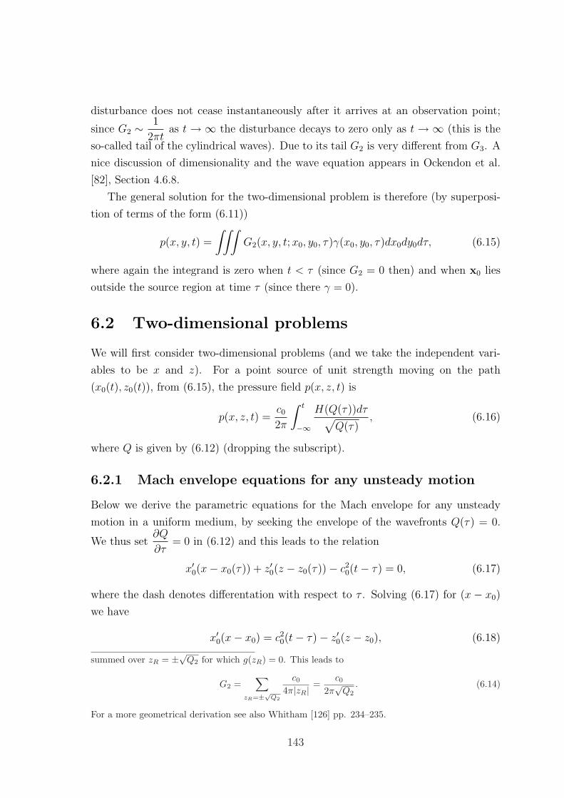
disturbance does not cease instantaneously after it arrives at an observation point;
since G2 ∼ 1
2πtas t → ∞ the disturbance decays to zero only as t →∞ (this is the
so-called tail of the cylindrical waves). Due to its tail G2 is very different from G3. A
nice discussion of dimensionality and the wave equation appears in Ockendon et al.
[82], Section 4.6.8.
The general solution for the two-dimensional problem is therefore (by superposi-
tion of terms of the form (6.11))
p(x, y, t) =
∫∫∫G2(x, y, t;x0, y0, τ)γ(x0, y0, τ)dx0dy0dτ, (6.15)
where again the integrand is zero when t < τ (since G2 = 0 then) and when x0 lies
outside the source region at time τ (since there γ = 0).
6.2 Two-dimensional problems
We will first consider two-dimensional problems (and we take the independent vari-
ables to be x and z). For a point source of unit strength moving on the path
(x0(t), z0(t)), from (6.15), the pressure field p(x, z, t) is
p(x, z, t) =c02π
∫ t
−∞
H(Q(τ))dτ√Q(τ)
, (6.16)
where Q is given by (6.12) (dropping the subscript).
6.2.1 Mach envelope equations for any unsteady motion
Below we derive the parametric equations for the Mach envelope for any unsteady
motion in a uniform medium, by seeking the envelope of the wavefronts Q(τ) = 0.
We thus set∂Q
∂τ= 0 in (6.12) and this leads to the relation
x′0(x− x0(τ)) + z′0(z − z0(τ))− c20(t− τ) = 0, (6.17)
where the dash denotes differentation with respect to τ . Solving (6.17) for (x − x0)
we have
x′0(x− x0) = c20(t− τ)− z′0(z − z0), (6.18)
summed over zR = ±√Q2 for which g(zR) = 0. This leads to
G2 =∑
zR=±√Q2
c0
4π|zR| =c0
2π√
Q2. (6.14)
For a more geometrical derivation see also Whitham [126] pp. 234–235.
143
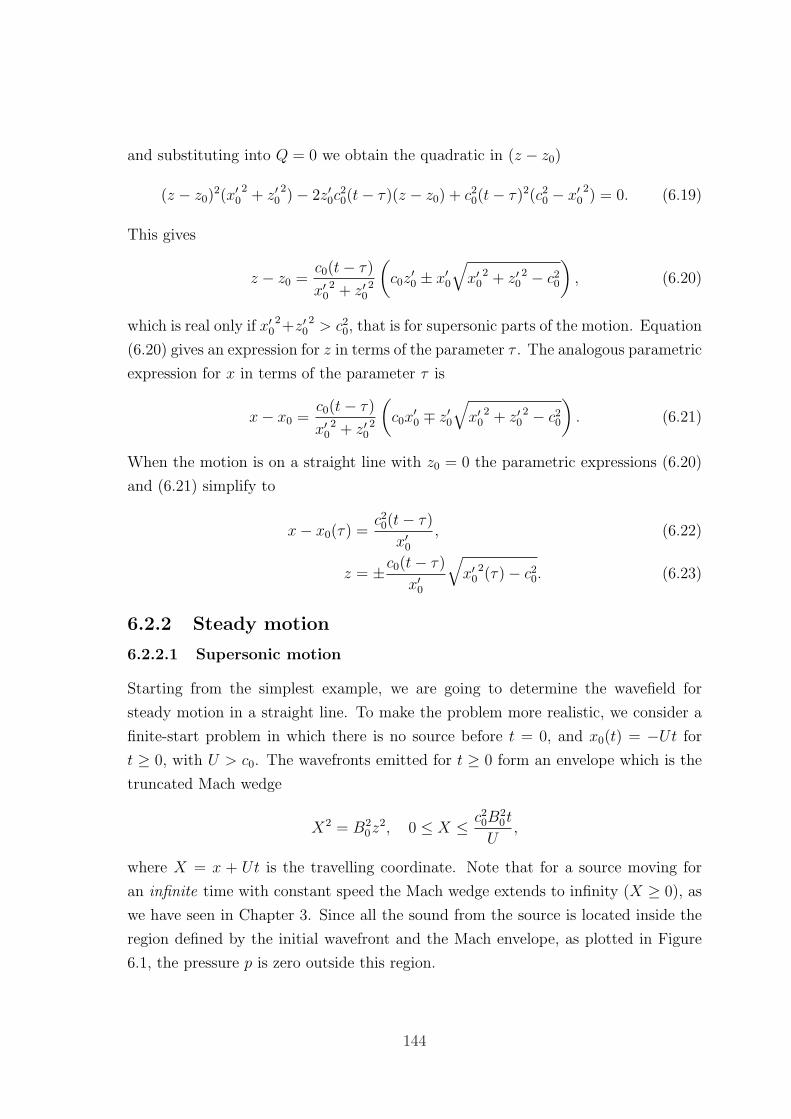
and substituting into Q = 0 we obtain the quadratic in (z − z0)
(z − z0)2(x′0
2+ z′0
2)− 2z′0c
20(t− τ)(z − z0) + c20(t− τ)2(c20 − x′0
2) = 0. (6.19)
This gives
z − z0 =c0(t− τ)
x′02 + z′0
2
(c0z
′0 ± x′0
√x′0
2 + z′02 − c20
), (6.20)
which is real only if x′02+z′0
2 > c20, that is for supersonic parts of the motion. Equation
(6.20) gives an expression for z in terms of the parameter τ . The analogous parametric
expression for x in terms of the parameter τ is
x− x0 =c0(t− τ)
x′02 + z′0
2
(c0x
′0 ∓ z′0
√x′0
2 + z′02 − c20
). (6.21)
When the motion is on a straight line with z0 = 0 the parametric expressions (6.20)
and (6.21) simplify to
x− x0(τ) =c20(t− τ)
x′0, (6.22)
z = ±c0(t− τ)
x′0
√x′0
2(τ)− c20. (6.23)
6.2.2 Steady motion
6.2.2.1 Supersonic motion
Starting from the simplest example, we are going to determine the wavefield for
steady motion in a straight line. To make the problem more realistic, we consider a
finite-start problem in which there is no source before t = 0, and x0(t) = −Ut for
t ≥ 0, with U > c0. The wavefronts emitted for t ≥ 0 form an envelope which is the
truncated Mach wedge
X2 = B20z
2, 0 ≤ X ≤ c20B20t
U,
where X = x + Ut is the travelling coordinate. Note that for a source moving for
an infinite time with constant speed the Mach wedge extends to infinity (X ≥ 0), as
we have seen in Chapter 3. Since all the sound from the source is located inside the
region defined by the initial wavefront and the Mach envelope, as plotted in Figure
6.1, the pressure p is zero outside this region.
144
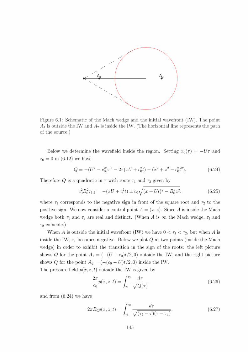
A1 A2
Figure 6.1: Schematic of the Mach wedge and the initial wavefront (IW). The pointA1 is outside the IW and A2 is inside the IW. (The horizontal line represents the pathof the source.)
Below we determine the wavefield inside the region. Setting x0(τ) = −Uτ and
z0 = 0 in (6.12) we have
Q = −(U2 − c20)τ2 − 2τ(xU + c20t)− (x2 + z2 − c20t
2). (6.24)
Therefore Q is a quadratic in τ with roots τ1 and τ2 given by
c20B20τ1,2 = −(xU + c20t)± c0
√(x+ Ut)2 −B2
0z2. (6.25)
where τ1 corresponds to the negative sign in front of the square root and τ2 to the
positive sign. We now consider a control point A = (x, z). Since A is inside the Mach
wedge both τ1 and τ2 are real and distinct. (When A is on the Mach wedge, τ1 and
τ2 coincide.)
When A is outside the initial wavefront (IW) we have 0 < τ1 < τ2, but when A is
inside the IW, τ1 becomes negative. Below we plot Q at two points (inside the Mach
wedge) in order to exhibit the transition in the sign of the roots: the left picture
shows Q for the point A1 = (−(U + c0)t/2, 0) outside the IW, and the right picture
shows Q for the point A2 = (−(c0 − U)t/2, 0) inside the IW.
The pressure field p(x, z, t) outside the IW is given by
2π
c0p(x, z, t) =
∫ τ2
τ1
dτ√Q(τ)
, (6.26)
and from (6.24) we have
2πB0p(x, z, t) =
∫ τ2
τ1
dτ√(τ2 − τ)(τ − τ1)
, (6.27)
145
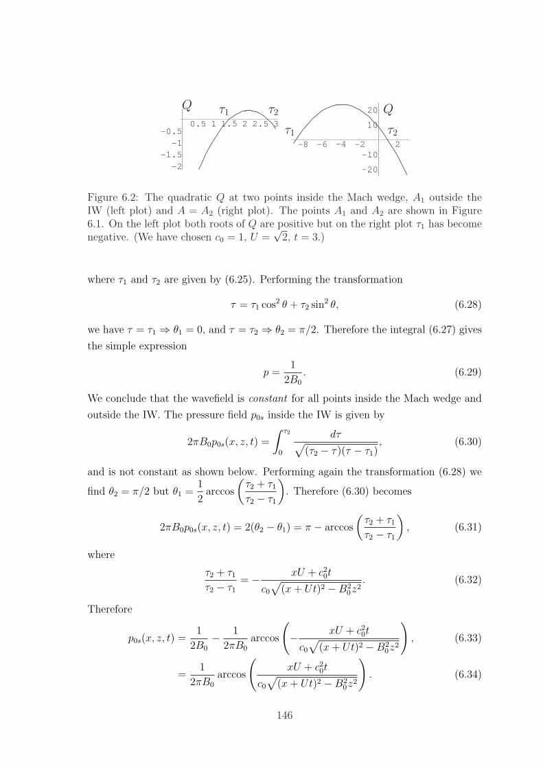
0.5 1 1.5 2 2.5 3
-2-1.5
-1-0.5
-8 -6 -4 -2 2
-20
-10
10
20 Q
τ1 τ2
τ2Q τ1
Figure 6.2: The quadratic Q at two points inside the Mach wedge, A1 outside theIW (left plot) and A = A2 (right plot). The points A1 and A2 are shown in Figure6.1. On the left plot both roots of Q are positive but on the right plot τ1 has becomenegative. (We have chosen c0 = 1, U =
√2, t = 3.)
where τ1 and τ2 are given by (6.25). Performing the transformation
τ = τ1 cos2 θ + τ2 sin2 θ, (6.28)
we have τ = τ1 ⇒ θ1 = 0, and τ = τ2 ⇒ θ2 = π/2. Therefore the integral (6.27) gives
the simple expression
p =1
2B0
. (6.29)
We conclude that the wavefield is constant for all points inside the Mach wedge and
outside the IW. The pressure field p0s inside the IW is given by
2πB0p0s(x, z, t) =
∫ τ2
0
dτ√(τ2 − τ)(τ − τ1)
, (6.30)
and is not constant as shown below. Performing again the transformation (6.28) we
find θ2 = π/2 but θ1 =1
2arccos
(τ2 + τ1τ2 − τ1
). Therefore (6.30) becomes
2πB0p0s(x, z, t) = 2(θ2 − θ1) = π − arccos
(τ2 + τ1τ2 − τ1
), (6.31)
where
τ2 + τ1τ2 − τ1
= − xU + c20t
c0√
(x+ Ut)2 −B20z
2. (6.32)
Therefore
p0s(x, z, t) =1
2B0
− 1
2πB0
arccos
(− xU + c20t
c0√
(x+ Ut)2 −B20z
2
), (6.33)
=1
2πB0
arccos
(xU + c20t
c0√
(x+ Ut)2 −B20z
2
). (6.34)
146
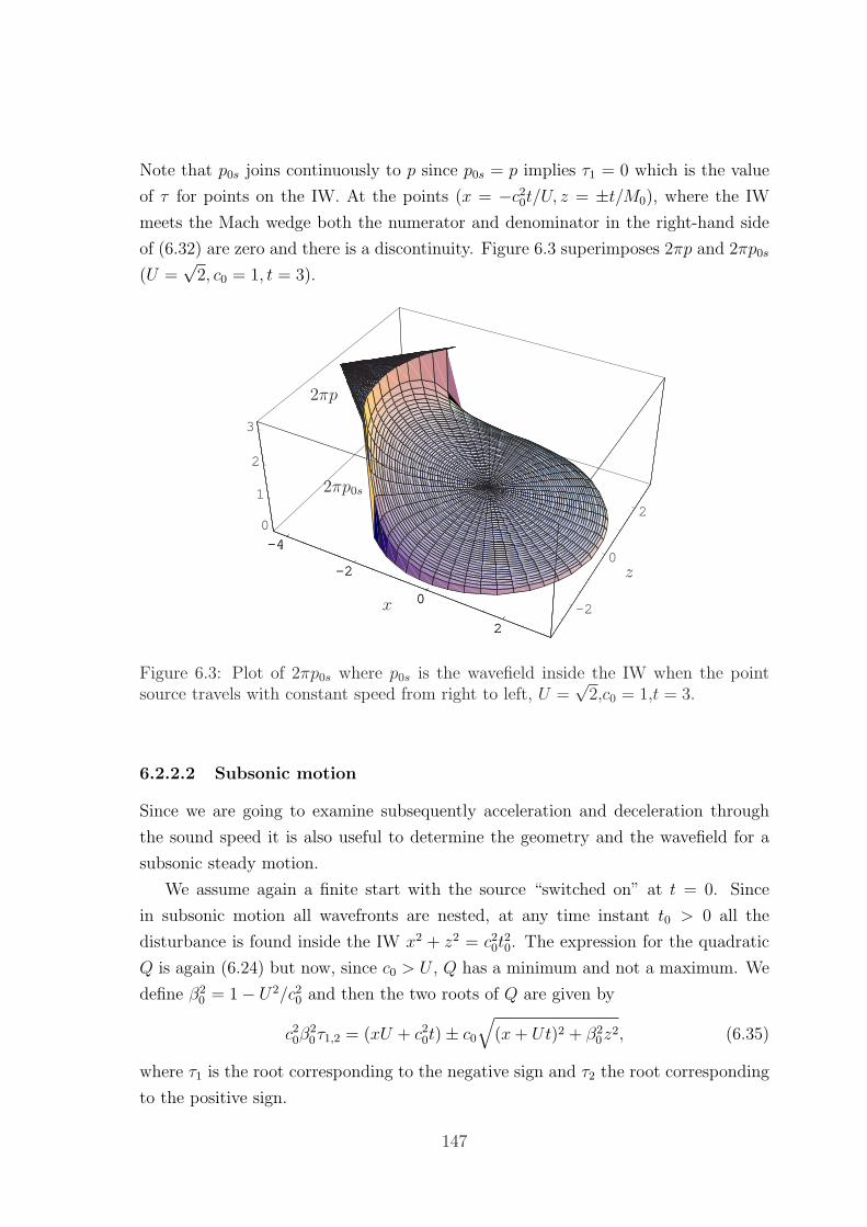
Note that p0s joins continuously to p since p0s = p implies τ1 = 0 which is the value
of τ for points on the IW. At the points (x = −c20t/U, z = ±t/M0), where the IW
meets the Mach wedge both the numerator and denominator in the right-hand side
of (6.32) are zero and there is a discontinuity. Figure 6.3 superimposes 2πp and 2πp0s
(U =√
2, c0 = 1, t = 3).
-4
-2
0
2
-2
0
20
1
2
3
-4
-2
0
2
x
z
2πp0s
2πp
Figure 6.3: Plot of 2πp0s where p0s is the wavefield inside the IW when the pointsource travels with constant speed from right to left, U =
√2,c0 = 1,t = 3.
6.2.2.2 Subsonic motion
Since we are going to examine subsequently acceleration and deceleration through
the sound speed it is also useful to determine the geometry and the wavefield for a
subsonic steady motion.
We assume again a finite start with the source “switched on” at t = 0. Since
in subsonic motion all wavefronts are nested, at any time instant t0 > 0 all the
disturbance is found inside the IW x2 + z2 = c20t20. The expression for the quadratic
Q is again (6.24) but now, since c0 > U , Q has a minimum and not a maximum. We
define β20 = 1− U2/c20 and then the two roots of Q are given by
c20β20τ1,2 = (xU + c20t)± c0
√(x+ Ut)2 + β2
0z2, (6.35)
where τ1 is the root corresponding to the negative sign and τ2 the root corresponding
to the positive sign.
147
Since (x + Ut)2 + β20z
2 > 0 for any point (x, z), the roots are always real and
distinct. This is equivalent to∂Q
∂τnot becoming zero (and consistent with the fact
that in subsonic motions no envelope of the wavefronts can be formed). The only
exception to this is the source position x = −Ut, z = 0 where∂Q
∂τand the roots
coalesce. Furthermore, when the point (x, z) is inside the IW the product and sum
of the roots are both positive so the roots are both positive.
Moreover, since the wavefronts are nested there is a unique τ1, satisfying 0 < τ1 <
t, at which Q = 0. Using this geometrical information the wavefield integral (6.7)
becomes
psub(x, z, t) =c02π
∫ τ1
0
dτ√Q
=1
2πβ0
∫ τ1
0
dτ√(τ1 − τ)(τ2 − τ)
. (6.36)
This can be calculated exactly if we let τ = τ1 cosh2 u− τ2 sinh2 u; we get
psub(x, z, t) =1
πβ0
∫ 0
−uL
du =1
πβ0
uL, (6.37)
where uL =1
2cosh−1
(τ1 + τ2τ2 − τ1
)and
τ1 + τ2τ2 − τ1
=xU + c20t
c0√
(x+ Ut)2 + β20z
2. (6.38)
From the last expression we find, as expected, that the wavefield is infinite at the
source.
In order to see the precise nature of the singularity, we consider points near the
source, with x = −Ut+ r cosφ, z = r sinφ where r is small. From (6.35) we have
c20β20τ1,2 = c20β
20t+ rU cosφ± rc0
√cos2 φ+ β2
0 sin2 φ. (6.39)
Using (6.39) in (6.37)–(6.38) we obtain
psource =1
2πβ0
cosh−1
(c20β
20t+ rU cosφ
c0r√
cos2 φ+ β20 sin2 φ
). (6.40)
Therefore as r → 0 we have
psource ∼ 1
2πβ0
ln
(2tc0β
20
r√
cos2 φ+ β20 sin2 φ
), (6.41)
which gives a logarithmic singularity as r → 0. The analogous three-dimensional
calculation can be found in Goldstein [44] pp. 45–50.
148
6.2.3 Acceleration through the sound speed
We now consider a point source accelerating through the sound speed—a problem
of great interest in sonic boom research since any supersonic vehicle must do this.
Flight tests, recorded in [123], indicate that acceleration through the sound speed
leads to the formation of a focused boom with amplitudes 2 to 5 times that of a
primary boom. It is a well-known fact in the early sonic boom literature that an
envelope of boomrays is formed during such a motion. In agreement with the more
recent sonic boom literature and the earlier parts of this thesis we will be calling this
envelope of boomrays a fold caustic. This fold caustic corresponds to the formation
of a cusp on the Mach envelope. These cusps had been reported as novel features in
the 1953 paper by Lilley et al. [73] and their position had been determined there.2
We feel that, up to now, the connection of these cusps to the fold caustic has not
been illustrated clearly nor explained adequately and we will strive to achieve both
these tasks below.
Furthermore, in Rosales and Tabak [109] when caustics of linear waves are re-
viewed it is shown that a Hilbert transform relates the waves before focusing to those
after focusing. The waves before focusing are called “incident” and the waves after
focusing are called “reflected”.3 There it is emphasised that a simple discontinuity
“converts” through the Hilbert transform to a logarithmic singularity. The latter
work employed high-frequency approximations.
However, as far as we know, no global approximation of the amplitude was made
in the literature. Below we also pursue this task, using the full linear wave theory
and working in the time domain.4 We find that significant progress can be made
analytically: using our detailed exposition of the underlying geometry we locate and
identify the singularities of the linear solution. This breakdown of the linear theory
indicates that the underlying small-amplitude approximation is no longer valid and
indicates that nonlinear effects should be introduced. However, the introduction of
nonlinearities in this problem is not an easy task. For a discussion of the introduc-
tion of nonlinear effects when modelling the focusing of weak shock waves we refer
the reader to Section 3.9; we recall from there that the current consensus in the
literature is that a nonlinear Tricomi equation should be solved to get the correct
2Also, the wavefront patterns were confirmed with experiments in a shallow water tank, makinguse of the ’hydraulic’ analogy.
3We have already used these terms in Chapter 3 and we will also be using them here.4We found after this work was completed that the method we use has close connections with the
time-domain method of Friedlander, in [40], pp. 67–70. Also, it would be interesting to explore theconnection of our work to the time-domain method used by Chapman in [22].
149
amplitudes near a fold caustic. This equation has been recently solved numerically
by Coulouvrat et al. for the scenario of constant-acceleration of a supersonic aircraft
[27]. However, in the next chapter, we will take a different approach and we will
investigate mainly analytically the re-introduction of nonlinear terms for a simpler
one-dimensional problem but one which is already quite complicated in its own right.
If the acceleration is a constant α and we scale time with c0/α and space with
c20/α then we get a dimensionless problem in which the sound speed and acceleration
are both equal to 1. So x0(t) = −t2/2, and we assume z0 = 0. We define U(t) = x′0(t)
to be the velocity, M0(t) = |U(t)| the Mach number, and B0(t) =√M2
0 − 1 the
Prandtl-Glauert parameter. For the motion under consideration U(t) = t, M0(t) = t
and B0(t) =√t2 − 1; the motion becomes supersonic at t = 1.
• Geometry
Below we discuss algebraically and geometrically the structure of the Mach envelope.
A discussion of the geometrical features can be found in [73, 102] and the Appendix
of [91], but we believe that the exposition here brings a better understanding as
it clarifies how this geometrical structure is related to the appearance of certain
logarithmic singularities in the wavefield and the associated breakdown of the linear
theory.
Now, from (6.12) the wavefronts are given by
Q(x, z; t, τ) = (t− τ)2 −(x+
1
2τ 2
)2
− z2 = 0, (6.42)
so Q is quartic in τ , and quadratic in x, z and t. From (6.22) and (6.23) the parametric
equations describing the Mach envelope are
xE(τ, t) = −1
2τ 2 −
(t− τ
τ
), (6.43)
zE(τ, t) = ±(t− τ)
(1− 1
τ 2
)1/2
, (6.44)
in the range 1 ≤ τ ≤ t. It is possible to eliminate τ from (6.43) and (6.44) and the
resulting equation for the envelope is cubic in t2 and z2 and quartic in x, but we shall
find the parametric form more convenient.
In Figure 6.4 we plot the Mach envelope for t = 1.2, 1.5, 2, 3. When t? = 2 the
source catches up with the disturbance it sent out at τ = 0 so we also plot the
wavefront x2 + z2 = t2?. In Figure 6.4 we can see that the Mach envelope has two
cusps which join a wedge-like part of the envelope with an arc-like part. These two
150
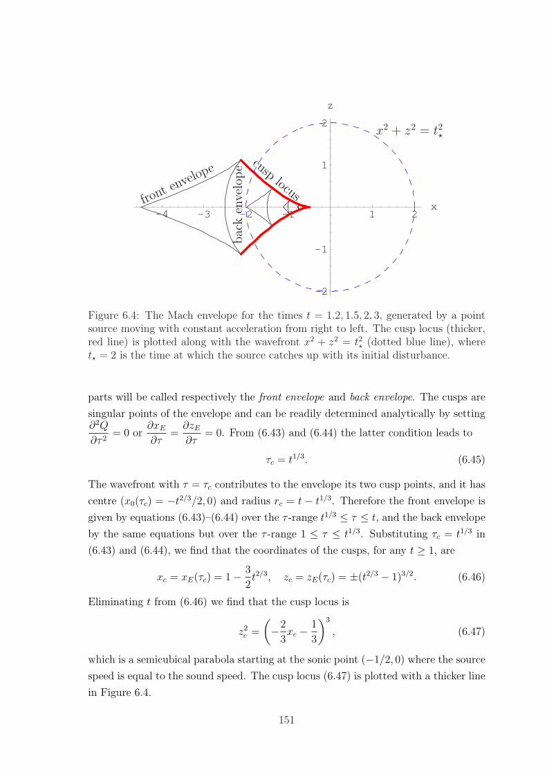
-4 -3 -2 -1 1 2x
-2
-1
1
2
z
bac
ken
velo
pe
x2 + z2 = t2?
front env
elope
cusplocus
Figure 6.4: The Mach envelope for the times t = 1.2, 1.5, 2, 3, generated by a pointsource moving with constant acceleration from right to left. The cusp locus (thicker,red line) is plotted along with the wavefront x2 + z2 = t2? (dotted blue line), wheret? = 2 is the time at which the source catches up with its initial disturbance.
parts will be called respectively the front envelope and back envelope. The cusps are
singular points of the envelope and can be readily determined analytically by setting∂2Q
∂τ 2= 0 or
∂xE∂τ
=∂zE∂τ
= 0. From (6.43) and (6.44) the latter condition leads to
τc = t1/3. (6.45)
The wavefront with τ = τc contributes to the envelope its two cusp points, and it has
centre (x0(τc) = −t2/3/2, 0) and radius rc = t − t1/3. Therefore the front envelope is
given by equations (6.43)–(6.44) over the τ -range t1/3 ≤ τ ≤ t, and the back envelope
by the same equations but over the τ -range 1 ≤ τ ≤ t1/3. Substituting τc = t1/3 in
(6.43) and (6.44), we find that the coordinates of the cusps, for any t ≥ 1, are
xc = xE(τc) = 1− 3
2t2/3, zc = zE(τc) = ±(t2/3 − 1)3/2. (6.46)
Eliminating t from (6.46) we find that the cusp locus is
z2c =
(−2
3xc − 1
3
)3
, (6.47)
which is a semicubical parabola starting at the sonic point (−1/2, 0) where the source
speed is equal to the sound speed. The cusp locus (6.47) is plotted with a thicker line
in Figure 6.4.
151
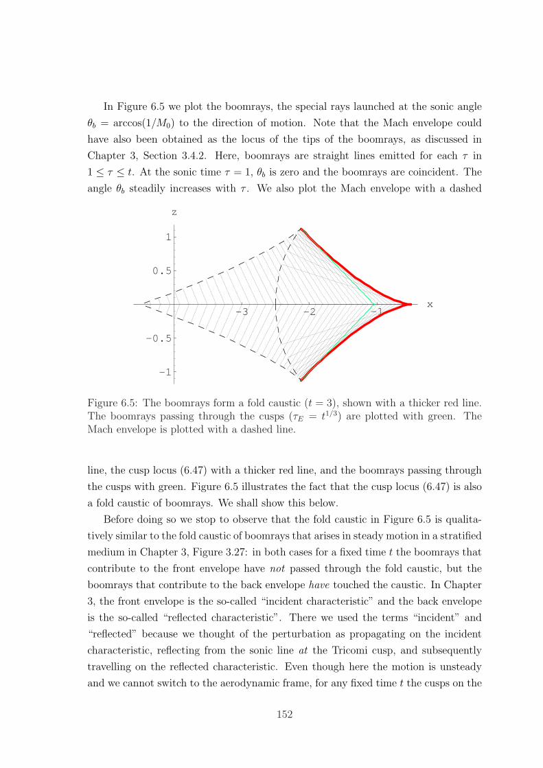
In Figure 6.5 we plot the boomrays, the special rays launched at the sonic angle
θb = arccos(1/M0) to the direction of motion. Note that the Mach envelope could
have also been obtained as the locus of the tips of the boomrays, as discussed in
Chapter 3, Section 3.4.2. Here, boomrays are straight lines emitted for each τ in
1 ≤ τ ≤ t. At the sonic time τ = 1, θb is zero and the boomrays are coincident. The
angle θb steadily increases with τ . We also plot the Mach envelope with a dashed
-3 -2 -1x
-1
-0.5
0.5
1
z
Figure 6.5: The boomrays form a fold caustic (t = 3), shown with a thicker red line.The boomrays passing through the cusps (τE = t1/3) are plotted with green. TheMach envelope is plotted with a dashed line.
line, the cusp locus (6.47) with a thicker red line, and the boomrays passing through
the cusps with green. Figure 6.5 illustrates the fact that the cusp locus (6.47) is also
a fold caustic of boomrays. We shall show this below.
Before doing so we stop to observe that the fold caustic in Figure 6.5 is qualita-
tively similar to the fold caustic of boomrays that arises in steady motion in a stratified
medium in Chapter 3, Figure 3.27: in both cases for a fixed time t the boomrays that
contribute to the front envelope have not passed through the fold caustic, but the
boomrays that contribute to the back envelope have touched the caustic. In Chapter
3, the front envelope is the so-called “incident characteristic” and the back envelope
is the so-called “reflected characteristic”. There we used the terms “incident” and
“reflected” because we thought of the perturbation as propagating on the incident
characteristic, reflecting from the sonic line at the Tricomi cusp, and subsequently
travelling on the reflected characteristic. Even though here the motion is unsteady
and we cannot switch to the aerodynamic frame, for any fixed time t the cusps on the
152
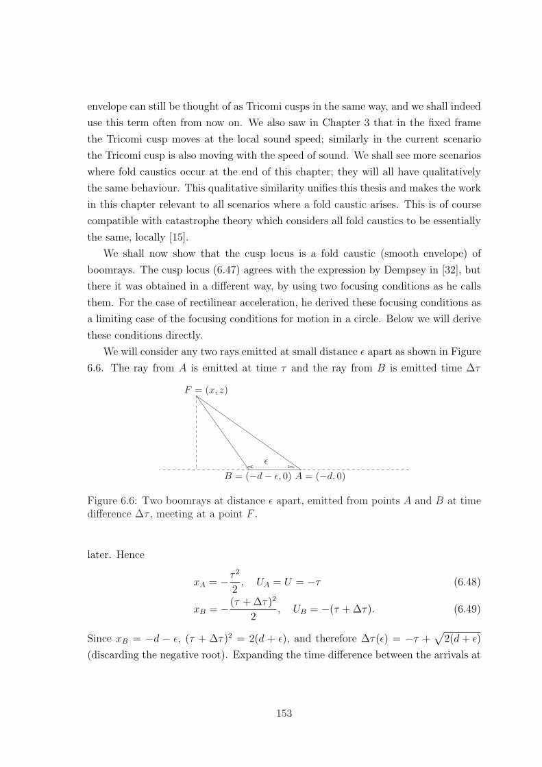
envelope can still be thought of as Tricomi cusps in the same way, and we shall indeed
use this term often from now on. We also saw in Chapter 3 that in the fixed frame
the Tricomi cusp moves at the local sound speed; similarly in the current scenario
the Tricomi cusp is also moving with the speed of sound. We shall see more scenarios
where fold caustics occur at the end of this chapter; they will all have qualitatively
the same behaviour. This qualitative similarity unifies this thesis and makes the work
in this chapter relevant to all scenarios where a fold caustic arises. This is of course
compatible with catastrophe theory which considers all fold caustics to be essentially
the same, locally [15].
We shall now show that the cusp locus is a fold caustic (smooth envelope) of
boomrays. The cusp locus (6.47) agrees with the expression by Dempsey in [32], but
there it was obtained in a different way, by using two focusing conditions as he calls
them. For the case of rectilinear acceleration, he derived these focusing conditions as
a limiting case of the focusing conditions for motion in a circle. Below we will derive
these conditions directly.
We will consider any two rays emitted at small distance ε apart as shown in Figure
6.6. The ray from A is emitted at time τ and the ray from B is emitted time ∆τ
ε
F = (x, z)
A = (−d, 0)B = (−d− ε, 0)
Figure 6.6: Two boomrays at distance ε apart, emitted from points A and B at timedifference ∆τ , meeting at a point F .
later. Hence
xA = −τ2
2, UA = U = −τ (6.48)
xB = −(τ + ∆τ)2
2, UB = −(τ + ∆τ). (6.49)
Since xB = −d − ε, (τ + ∆τ)2 = 2(d + ε), and therefore ∆τ(ε) = −τ +√
2(d+ ε)
(discarding the negative root). Expanding the time difference between the arrivals at
153
F , tBF + ∆τ(ε)− tAF as a series in powers of ε we find
tBF + ∆τ(ε)− tAF =ε
(1
τ+
x+ d√(x+ d)2 + z2
)+
ε2
2
(− 1
τ 3− (x+ d)2
((x+ d)2 + z2)3/2+
1√(x+ d)2 + z2
)+
ε3
2
(1
τ 5+
(x+ d)3
((x+ d)2 + z2)5/2− x+ d
((x+ d)2 + z2)3/2
)+O(ε4).
(6.50)
Setting the coefficient of the order ε term to zero we recover the boomray condition
cos θb =1
|U | (discussed in Chapter 3) where θb is the acute angle between AF and
AB. The boomray condition can be thought of as a “first-order focusing condition”
for the rays. Now, we look for an envelope of boomrays by setting the coefficient of
the order ε2 term to zero. From the resulting relation and the boomray condition, we
obtain the “second-order focusing condition”
x+ d = −U2 sin2 θb. (6.51)
For the points such that the boomray condition and condition (6.51) are satisfied, the
boomray signals arrive with a time difference of order ε3. Eliminating τ from these
two conditions we obtain again the cusp locus expression (6.47). So we have proved
that the cusp locus is a curve of second-order focusing. Furthermore, the coefficient
of ε3 is always positive so in a constant acceleration motion we cannot have any focus
of order higher than second.
Wavefront pattern
In this section we will discusss the wavefront pattern further, and explain how a
wavefront emitted at time t = τ ≥ 1 contributes to the Mach envelope. In Figure
6.7 we plot the wavefronts for various values of τ in the interval 0 ≤ τ ≤ t when
t = 3; we also plot the cusp locus with a thicker, red line. We observe a distinct
geometrical difference between the front and the back envelope; the t1/3 ≤ τ ≤ t
wavefronts envelope the front envelope from the inside, that is the front envelope is
formed in a similar way to the Mach wedge, but the 1 ≤ τ ≤ t1/3 wavefronts envelope
the back envelope from the outside. This difference is shown more clearly in the
schematic diagrams of Figure 6.8. An algebraic criterion for distinguishing the two
types of envelope formation appears also below. In Chapter 3, the same qualitative
change took place in the wavefront pattern associated with a fold caustic of boomrays:
154
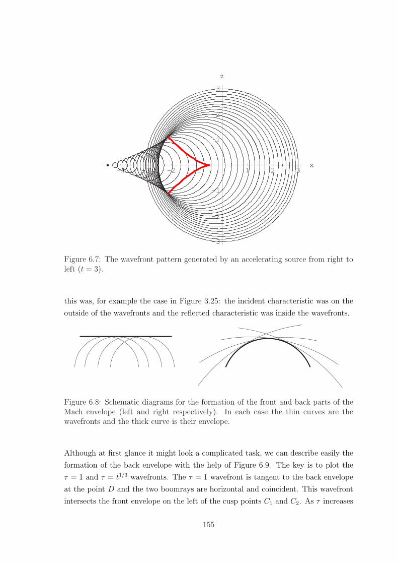
-4 -3 -2 -1 1 2 3x
-3
-2
-1
1
2
3
z
Figure 6.7: The wavefront pattern generated by an accelerating source from right toleft (t = 3).
this was, for example the case in Figure 3.25: the incident characteristic was on the
outside of the wavefronts and the reflected characteristic was inside the wavefronts.
Figure 6.8: Schematic diagrams for the formation of the front and back parts of theMach envelope (left and right respectively). In each case the thin curves are thewavefronts and the thick curve is their envelope.
Although at first glance it might look a complicated task, we can describe easily the
formation of the back envelope with the help of Figure 6.9. The key is to plot the
τ = 1 and τ = t1/3 wavefronts. The τ = 1 wavefront is tangent to the back envelope
at the point D and the two boomrays are horizontal and coincident. This wavefront
intersects the front envelope on the left of the cusp points C1 and C2. As τ increases
155
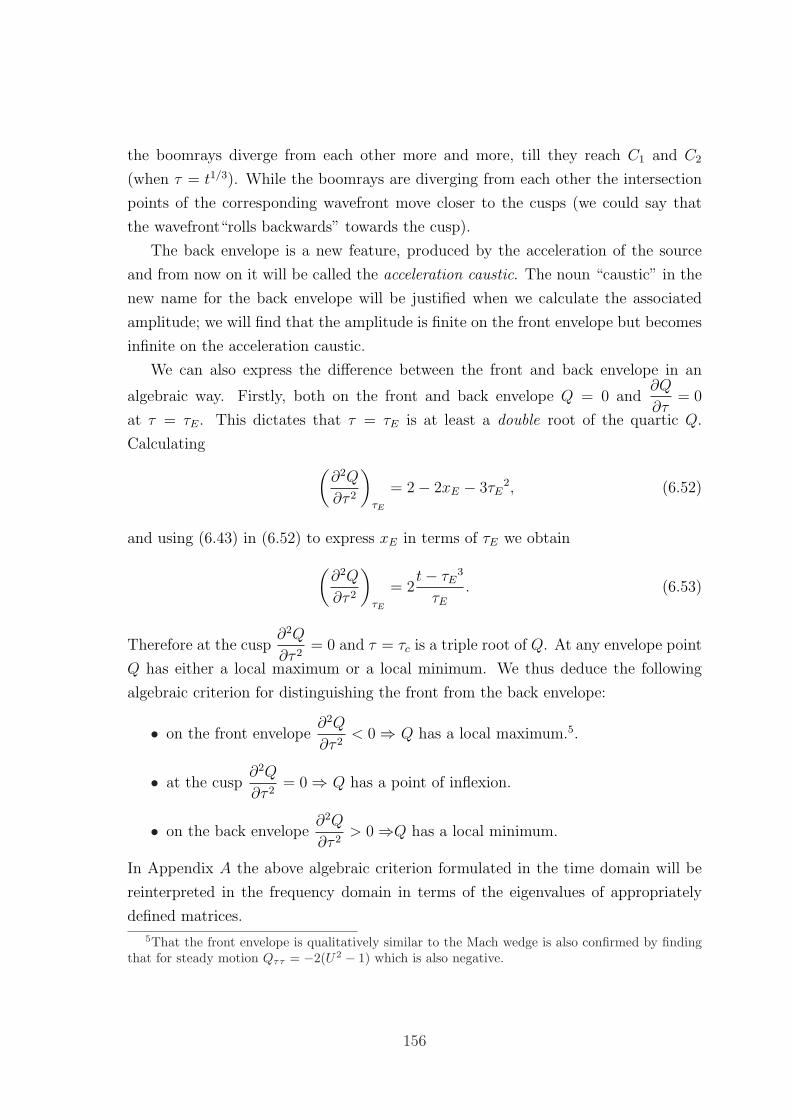
the boomrays diverge from each other more and more, till they reach C1 and C2
(when τ = t1/3). While the boomrays are diverging from each other the intersection
points of the corresponding wavefront move closer to the cusps (we could say that
the wavefront“rolls backwards” towards the cusp).
The back envelope is a new feature, produced by the acceleration of the source
and from now on it will be called the acceleration caustic. The noun “caustic” in the
new name for the back envelope will be justified when we calculate the associated
amplitude; we will find that the amplitude is finite on the front envelope but becomes
infinite on the acceleration caustic.
We can also express the difference between the front and back envelope in an
algebraic way. Firstly, both on the front and back envelope Q = 0 and∂Q
∂τ= 0
at τ = τE. This dictates that τ = τE is at least a double root of the quartic Q.
Calculating
(∂2Q
∂τ 2
)
τE
= 2− 2xE − 3τE2, (6.52)
and using (6.43) in (6.52) to express xE in terms of τE we obtain
(∂2Q
∂τ 2
)
τE
= 2t− τE
3
τE. (6.53)
Therefore at the cusp∂2Q
∂τ 2= 0 and τ = τc is a triple root of Q. At any envelope point
Q has either a local maximum or a local minimum. We thus deduce the following
algebraic criterion for distinguishing the front from the back envelope:
• on the front envelope∂2Q
∂τ 2< 0 ⇒ Q has a local maximum.5.
• at the cusp∂2Q
∂τ 2= 0 ⇒ Q has a point of inflexion.
• on the back envelope∂2Q
∂τ 2> 0 ⇒Q has a local minimum.
In Appendix A the above algebraic criterion formulated in the time domain will be
reinterpreted in the frequency domain in terms of the eigenvalues of appropriately
defined matrices.
5That the front envelope is qualitatively similar to the Mach wedge is also confirmed by findingthat for steady motion Qττ = −2(U2 − 1) which is also negative.
156
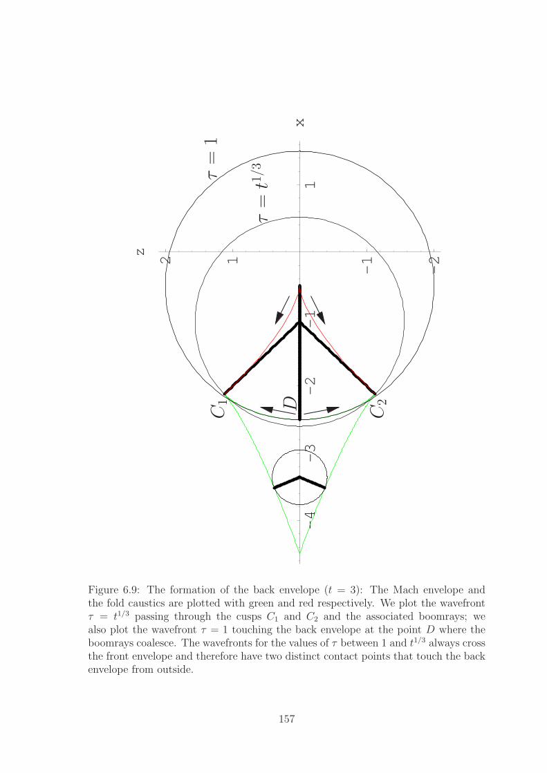
-4
-3
-2
-1
1x
-2
-112z
τ=t1/3
D
τ=
1C
1
C2
Figure 6.9: The formation of the back envelope (t = 3): The Mach envelope andthe fold caustics are plotted with green and red respectively. We plot the wavefrontτ = t1/3 passing through the cusps C1 and C2 and the associated boomrays; wealso plot the wavefront τ = 1 touching the back envelope at the point D where theboomrays coalesce. The wavefronts for the values of τ between 1 and t1/3 always crossthe front envelope and therefore have two distinct contact points that touch the backenvelope from outside.
157
Since the amplitude is proportional to
∫ t
0
H(Q(τ))dτ√Q(τ)
, the aforementioned differ-
ence in the behaviour of Q directly relates to corresponding differences in the ampli-
tudes at the front envelope, the back envelope, and the cusp. We will investigate this
in detail in the next section.
•Wavefield
We have plotted above the wavefront pattern and Mach envelope associated with
constant acceleration through the sound speed and we have discussed their features.
Using that information, we are now going to approximate appropriately the wavefield
integral (6.16) near the front envelope, near the acceleration caustic and near the
cusp. (In Section 6.2.4 we will extend the same method to calculate approximate
amplitudes near the Mach envelope for a motion with constant deceleration through
the sound speed.)
The wavefield at a certain point (x, z) is determined by the integral (6.16). For a
moving point source of unit strength that starts moving at time τ = 0, no contribution
comes from values of t that are less than zero. Also when (x, z) is outside the Mach
envelope and outside the IW, as explained above, Q < 0 and p = 0. Therefore, to
summarise, the integral (6.16) is defined only over the first quadrant of the Q-τ plane.
Since Q is a quartic the limits of integration are more difficult to determine alge-
braically than those of the steady motion. It would be possible to obtain an expression
for p everywhere in the region of influence, in terms of standard elliptic integrals, but
we will not do this here as it is unnecessarily complicated. To determine only the
singular part of the wavefield near the Mach envelope that is associated with the
sonic boom it is enough to perform a simple approximation on the integral. On the
envelope Q has either a double or triple root so we can determine all four of its roots
analytically. Expanding Q from (6.42) as a polynomial in τ we obtain
−4Q(τ, x, z, t) = τ 4 − 4(1− x)τ 2 + 8tτ − 4(t2 − x2 − z2). (6.54)
For any envelope point, since τ = τE is a double root, Q satisfies the relation
−4Q = (τ − τE)2g(τ) where g(τ) = (τ − τ3)(τ − τ4). (6.55)
Therefore
Sum of roots = SQ = 2τE + τ3x+ τ4 = 0, (6.56)
Product of roots = PQ = τ 2Eτ1τ4 = 4(x2
E + z2E − t2). (6.57)
158
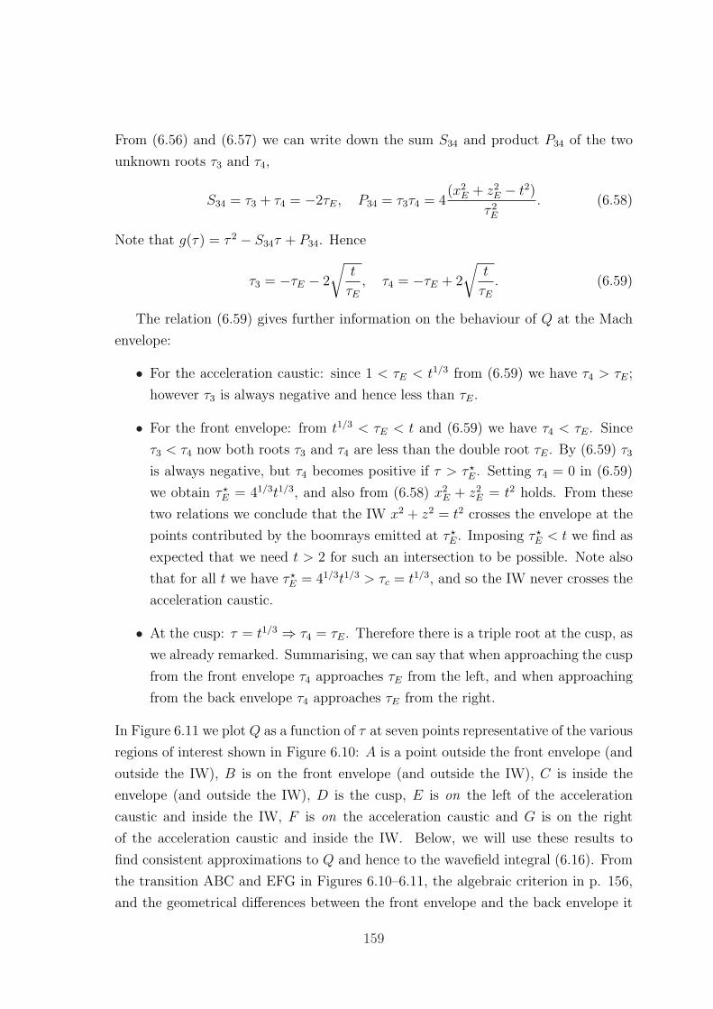
From (6.56) and (6.57) we can write down the sum S34 and product P34 of the two
unknown roots τ3 and τ4,
S34 = τ3 + τ4 = −2τE, P34 = τ3τ4 = 4(x2
E + z2E − t2)
τ 2E
. (6.58)
Note that g(τ) = τ 2 − S34τ + P34. Hence
τ3 = −τE − 2
√t
τE, τ4 = −τE + 2
√t
τE. (6.59)
The relation (6.59) gives further information on the behaviour of Q at the Mach
envelope:
• For the acceleration caustic: since 1 < τE < t1/3 from (6.59) we have τ4 > τE;
however τ3 is always negative and hence less than τE.
• For the front envelope: from t1/3 < τE < t and (6.59) we have τ4 < τE. Since
τ3 < τ4 now both roots τ3 and τ4 are less than the double root τE. By (6.59) τ3
is always negative, but τ4 becomes positive if τ > τ ?E. Setting τ4 = 0 in (6.59)
we obtain τ ?E = 41/3t1/3, and also from (6.58) x2E + z2
E = t2 holds. From these
two relations we conclude that the IW x2 + z2 = t2 crosses the envelope at the
points contributed by the boomrays emitted at τ ?E. Imposing τ ?E < t we find as
expected that we need t > 2 for such an intersection to be possible. Note also
that for all t we have τ ?E = 41/3t1/3 > τc = t1/3, and so the IW never crosses the
acceleration caustic.
• At the cusp: τ = t1/3 ⇒ τ4 = τE. Therefore there is a triple root at the cusp, as
we already remarked. Summarising, we can say that when approaching the cusp
from the front envelope τ4 approaches τE from the left, and when approaching
from the back envelope τ4 approaches τE from the right.
In Figure 6.11 we plot Q as a function of τ at seven points representative of the various
regions of interest shown in Figure 6.10: A is a point outside the front envelope (and
outside the IW), B is on the front envelope (and outside the IW), C is inside the
envelope (and outside the IW), D is the cusp, E is on the left of the acceleration
caustic and inside the IW, F is on the acceleration caustic and G is on the right
of the acceleration caustic and inside the IW. Below, we will use these results to
find consistent approximations to Q and hence to the wavefield integral (6.16). From
the transition ABC and EFG in Figures 6.10–6.11, the algebraic criterion in p. 156,
and the geometrical differences between the front envelope and the back envelope it
159
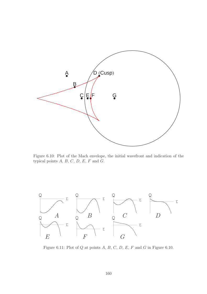
A
B
C
D HCuspLE F G
Figure 6.10: Plot of the Mach envelope, the initial wavefront and indication of thetypical points A, B, C, D, E, F and G.
ΤQ
Τ
Q
Τ
Q
ΤQ
ΤQ
ΤQ
ΤQ
A B C D
E F G
Figure 6.11: Plot of Q at points A, B, C, D, E, F and G in Figure 6.10.
160
is obvious that the wavefield on the back envelope is of a different nature from the
wavefield on the front envelope.
Let us take a general point (xE, zE) anywhere on the envelope (with t considered
a fixed parameter). Since the acceleration caustic is never parallel to the x-axis we
will keep zE fixed and we will obtain the approximation to the wavefield integral
as a function of x where |x − xE| is small. The small parameter of the asymptotic
procedure will be taken to be proportional to |x− xE|α where α is greater than zero
and to be determined.
Under the assumption of |x−xE| being small, the quartic Q will be approximated
with lower-order polynomials, while retaining in each region its most important fea-
tures. Roughly the idea of the approximation method we will use is the following:
since Q has a local maximum/minimum at any front/back envelope point, two roots
of Q are enough to reconstruct the local behaviour and Q will be approximated with
a quadratic there; Q will be approximated with a cubic near the cusp since it has a
point of inflexion there and three roots are in play. These approximations for Q will
enable us to find approximations to the amplitude analytically.
We consider any point near the envelope and expand Q(τ, x; zE, t) in a Taylor
series about the envelope point (τE, xE; zE, t), using Q =∂Q
∂τ= 0 on the envelope.
We obtain
Q(τ, x; zE, t) =
(∂Q
∂x
)
E
(x− xE) +1
2
(∂2Q
∂τ 2
)
E
(τ − τE)2 + h.o.t (6.60)
We let
C1 =
(∂Q
∂x
)
E
= −2xE − τ 2E = 2
t− τEτE
> 0 for 1 ≤ τ ≤ t, (6.61)
and C2 =1
2
(∂2Q
∂τ 2
)
E
=t− τ 3
E
τE
{< 0 for t1/3 ≤ τE ≤ t> 0 for t ≤ τE ≤ 1.
(6.62)
So, from (6.60) we conclude that for any point (x, z) near the envelope with ε2 ∼|x− xE| the τ -roots of Q are perturbed by O(ε). We will denote the perturbed roots
by τ ′1, τ′2, τ
′3 and τ ′4.
¦ Wavefield near the front envelope
We pick the point (xE, zE) on the front envelope. We will consider points at small
distance |x− xE| from this point. Without loss of generality, we can take (xE, zE) so
that τE ≥ 41/3t1/3 so that the wavefield outside the envelope is zero.6
6At a point on the front envelope but inside the IW, there is an extra contribution to the
161
From the general expression (6.16) and using (6.60), (6.61) and (6.62), we obtain
for x > xE (see plot C in Figure 6.11)
2πp(x; zE, t) ∼ 1√|C2|
∫ τ ′2
τ ′1
dτ√(τ ′2 − τ)(τ − τ ′1)
, (6.63)
where
τ ′1 = τE −√C1
C2
(xE − x),
τ ′2 = τE +
√C1
C2
(xE − x).
The roots τ ′3 and τ ′4 are both negative.
From the calculations for steady motion (6.27)–(6.29) the integral (6.63) immedi-
ately evaluates to
p(x, zE, t) ∼ 1
2√|C2|
. (6.64)
Hence, as x→ xE the pressure jump across the front envelope is given by
p(x+E, zE, t)− 0 =
1
2√|C2|
=1
2
(τE
τ 3E − t
)1/2
. (6.65)
We plot the jump (6.65) in Figure 6.12 for t1/3 ≤ τE ≤ t− 0.001. The jump near the
source, as τE → t, is
p(t, t) =1
2
1√t2 − 1
. (6.66)
Since the local Prandtl-Glauert parameter B0 =√τ 2 − 1 takes the value
√t2 − 1
in the limit τE → t, (6.66) agrees with the steady motion result (6.29) and provides
another verification of the similarity between the Mach wedge and the front envelope.
However as τE → t1/3 the jump tends to infinity. This indicates that the quadratic
approximation for Q is insufficient at the cusp and more terms would need to be
retained in the Taylor series (6.60) for Q. We leave the analysis of the wavefield near
the cusp for later.
wavefield, given by∫ τ ′4
0
dτ√Q
(see plot E in Figure 6.11). However, this contribution is continuous
across the envelope and since we are interested in the abrupt jump in the wavefield due to the
singular contribution∫ τ ′2
τ ′1
dτ√Q
we do not lose any generality by considering points outside the IW.
162
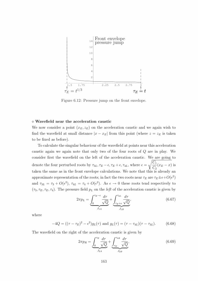
1.5 1.75 2.25 2.5 2.75 3
2
4
6
8
10
12
14Front envelopepressure jump
τE = t1/3 τE = tτE = t
Figure 6.12: Pressure jump on the front envelope.
¦ Wavefield near the acceleration caustic
We now consider a point (xE, zE) on the acceleration caustic and we again wish to
find the wavefield at small distance |x − xE| from this point (where z = zE is taken
to be fixed as before).
To calculate the singular behaviour of the wavefield at points near this acceleration
caustic again we again note that only two of the four roots of Q are in play. We
consider first the wavefield on the left of the acceleration caustic. We are going to
denote the four perturbed roots by τ3L, τE − ε, τE + ε, τ4L, where ε =
√C1
C2
(xE − x) is
taken the same as in the front envelope calculations. We note that this is already an
approximate representation of the roots; in fact the two roots near τE are τE±ε+O(ε2)
and τ3L = τ3 + O(ε2), τ4L = τ4 + O(ε2). As ε → 0 these roots tend respectively to
(τ3, τE, τE, τ4). The pressure field pL on the left of the acceleration caustic is given by
2πpL =
∫ τE−ε
0
dτ√Q︸ ︷︷ ︸
J1A
+
∫ τ4L
τE+ε
dτ√Q︸ ︷︷ ︸
J1B
, (6.67)
where
−4Q = ((τ − τE)2 − ε2)gL(τ) and gL(τ) = (τ − τ4L)(τ − τ3L). (6.68)
The wavefield on the right of the acceleration caustic is given by
2πpR =
∫ τE
0
dτ√Q︸ ︷︷ ︸
J2A
+
∫ τ4R
τE
dτ√Q︸ ︷︷ ︸
J2B
, (6.69)
163
where
−4Q = ((τ − τE)2 + ε2)gR(τ) and gR(τ) = (τ − τ3R)(τ − τ4R). (6.70)
As ε→ 0, both gL(τ) and gR(τ) tend to g(τ).
We will first evaluate J1A and J2A and compare them as they both deal with the
range of integration 0 ≤ τ ≤ τE (see Figure 6.18, plot E). Firstly for
J1A =
∫ τE−ε
0
fL(τ)dτ√(τ − τE)2 − ε2
, (6.71)
where fL(τ) =
√−4
gL(τ), to extract the singular behaviour, we split the numerator as
fL(τ) = fL(τE) + (fL(τ)− fL(τE)): therefore
J1A =
∫ τE−ε
0
fL(τE)dτ√(τ − τE)2 − ε2︸ ︷︷ ︸J1A(i)
+
∫ τE−ε
0
(fL(τ)− fL(τE))dτ√(τ − τE)2 − ε2︸ ︷︷ ︸J1A(ii)
. (6.72)
The first integral J1A(i) contains the singular behaviour of J1A and J1A(ii) tends to
a finite limit as ε → 0 which is negligible in comparison with the singular part.
Therefore we have
J1A(i) = fL(τE) cosh−1(τEε
)(6.73)
= fL(τE) ln
(τEε
+
√(τEε
)2
− 1
), (6.74)
and as ε→ 0 we have
J1A(i) = f(τE) (− ln ε+ ln(2τE)) + o(1). (6.75)
Therefore J1A(i) gives rise to a logarithmic singularity of strength f(τE). Now, for
J1A(ii) =
∫ τE−ε
0
(fL(τ)− fL(τE))dτ√(τ − τE)2 − ε2
, (6.76)
letting ε→ 0 we obtain
J1A(ii) →∫ τE
0
(f(τ)− f(τE))dτ
(τE − τ), (6.77)
164
which is finite. Now, in the same fashion we have adopted for (6.72), we write
J2A =
∫ τE
0
fR(τE)dτ√(τ − τE)2 + ε2︸ ︷︷ ︸J2A(i)
+
∫ τE
0
(fR(τ)− fR(τE))dτ√(τ − τE)2 + ε2︸ ︷︷ ︸J2A(ii)
. (6.78)
Again, the first integral J2A(i) contains the singular behaviour of J2A and J2A(ii) tends
to a finite limit as ε→ 0. Now
J2A(i) = fR(τE) sinh−1(τEε
)(6.79)
= fR(τE) ln
(τEε
+
√(τEε
)2
+ 1
), (6.80)
and as ε→ 0 we have
J2A(i) = f(τE) (− ln ε+ ln(2τE)) + o(1). (6.81)
Therefore J2A(i) also gives rise to a logarithmic singularity of strength f(τE). We thus
conclude that the logarithmic singularities from J1A(i) and J2A(i), respectively on the
left and on the right of the acceleration caustic, are of equal strength. Lastly, letting
ε→ 0 in the finite part of J2A,
J2A(ii) =
∫ τE
0
(fR(τ)− fR(τE))dτ√(τ − τE)2 + ε2
, (6.82)
we have that
J2A(ii) →∫ τE
0
(f(τ)− f(τE))dτ
(τE − τ). (6.83)
Therefore we also conclude that as ε→ 0 the integrals J1A(ii) and J2A(ii) tend to the
same finite limit. This finite integral is negligible in comparison with the singular
part and we are not going to calculate it precisely.
The range of integration τE + ε ≤ τ ≤ τ4 is dealt with similarly. We find
J1B(i) = fL(τE) cosh−1
(τ4 − τE
ε
)(6.84)
= fL(τE) ln
τ4 − τE
ε+
√(τ4 − τE
ε
)2
− 1
, (6.85)
and as ε→ 0
J1B(i) = f(τE) (− ln ε+ ln(2(τ4 − τE))) + o(1). (6.86)
165
Also on the right of the acceleration caustic
J2B(i) = fR(τE) sinh−1
(τ4 − τE
ε
)(6.87)
= fR(τE) ln
τ4 − τE
ε+
√(τ4 − τE
ε
)2
+ 1
, (6.88)
and as ε→ 0
J2B(i) = f(τE) (− ln ε+ ln(2(τ4 − τE))) + o(1). (6.89)
We also find that as ε→ 0, J1B(ii) and J2B(ii) tend to the same finite limit∫ τ4
τE
(f(τ)− f(τE))dτ
(τ − τE). Since
J1 = J1A(i) + J1B(i) + J1A(ii) + J1B(ii), (6.90)
as ε→ 0, putting together all the results from above, we have
J1 = −2f(τE) ln(ε) +O(1), (6.91)
and similarly
J2 = J2A(i) + J2B(i) + J2A(ii) + J2B(ii). (6.92)
It remains to find f(τE) so that we can determine the strength of the logarithmic
singularities. Since
f(τE) =
√−4
g(τE), (6.93)
using (6.58) we obtain
f(τE; t) =
√τE
t− τ 3E
. (6.94)
Therefore f(τE) blows up as τE → t1/3. We plot f(τE) in Figure 6.13 for
1 ≤ τE ≤ t1/3 − 0.001. Note that at the point where boomrays coalesce, we have
f(1; t) =
√1
t− 1which is finite for any t > 1; this point has no other significance
beyond this fact. Comparing the jump on the front envelope and the strength of the
logarithmic singularity f(τE, t) we see that both involve the function
√τE
|t− τ 3E|
.
166

1.1 1.2 1.3 1.4
2
4
6
8
10
12
14
τEτE = 1 τE = t1/3
f(τE, t)
Figure 6.13: Plot of f(τE, t) as a function of τE, where −2f(τE, t) is the strength ofthe logarithmic singularity.
It is also of interest to determine how f(τE) is related to |z − zc| where zc is the
z-coordinate at the cusp and |z − zc| small. We find
f(τE) ∼ 1
61/4
(τ 2c − 1)−1/8
τc(zE − zc)
−1/4,
and using τc = t1/3 we have
f(τE) ∼ 1
61/4t−1/6(t2/3 − 1)−1/8(zE − zc)
−1/4. (6.95)
¦ Wavefield near the cusp
At the cusp the truncated Taylor series (6.60) is not a sufficient approximation since∂2Q
∂τ 2= 0. Still fixing our attention on points on a horizontal line z = zc, we retain
the next term up in the series in τ which is the term with∂3Q
∂τ 3= 0: we have
Q(τ, x; zc, t) =
(∂Q
∂x
)
c
(x− xc) +1
6
(∂3Q
∂τ 3
)
c
(τ − τc)3 + h.o.t, (6.96)
where
(∂Q
∂x
)
c
is given as a function of τ and t in (6.61) and
(∂2Q
∂τ 2
)
c
= −6τ . There-
fore we rewrite (6.96) as
Q(τ, x; zc, t) =2t− τEτE
(x− xc)− τc(τ − τc)3 + h.o.t. (6.97)
=C1(x− xc)− C3(τ − τc)3 + h.o.t. (6.98)
167
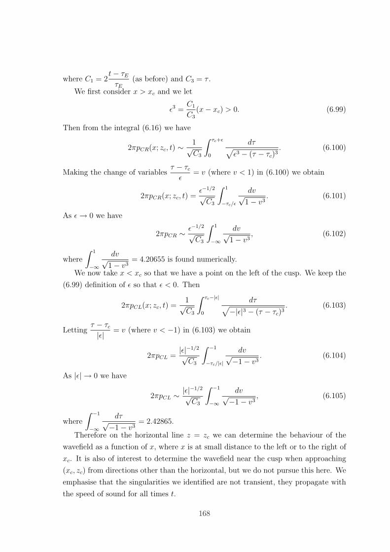
where C1 = 2t− τEτE
(as before) and C3 = τ .
We first consider x > xc and we let
ε3 =C1
C3
(x− xc) > 0. (6.99)
Then from the integral (6.16) we have
2πpCR(x; zc, t) ∼ 1√C3
∫ τc+ε
0
dτ√ε3 − (τ − τc)3
. (6.100)
Making the change of variablesτ − τcε
= v (where v < 1) in (6.100) we obtain
2πpCR(x; zc, t) =ε−1/2
√C3
∫ 1
−τc/ε
dv√1− v3
. (6.101)
As ε→ 0 we have
2πpCR ∼ ε−1/2
√C3
∫ 1
−∞
dv√1− v3
, (6.102)
where
∫ 1
−∞
dv√1− v3
= 4.20655 is found numerically.
We now take x < xc so that we have a point on the left of the cusp. We keep the
(6.99) definition of ε so that ε < 0. Then
2πpCL(x; zc, t) =1√C3
∫ τc−|ε|
0
dτ√−|ε|3 − (τ − τc)3
. (6.103)
Lettingτ − τc|ε| = v (where v < −1) in (6.103) we obtain
2πpCL =|ε|−1/2
√C3
∫ −1
−τc/|ε|
dv√−1− v3. (6.104)
As |ε| → 0 we have
2πpCL ∼ |ε|−1/2
√C3
∫ −1
−∞
dv√−1− v3, (6.105)
where
∫ −1
−∞
dτ√−1− v3= 2.42865.
Therefore on the horizontal line z = zc we can determine the behaviour of the
wavefield as a function of x, where x is at small distance to the left or to the right of
xc. It is also of interest to determine the wavefield near the cusp when approaching
(xc, zc) from directions other than the horizontal, but we do not pursue this here. We
emphasise that the singularities we identified are not transient, they propagate with
the speed of sound for all times t.
168

6.2.4 Deceleration through the sound speed
We now consider another motion of great practical relevance. We consider a point
source moving along the x-direction, from left to right in steady supersonic motion,
with M0 > 1 and which starts decelerating uniformly at τ = 0. We thus have that
x0(t) = M0t t ≤ 0, (6.106)
x0(t) = M0t− t2/2 0 ≤ t ≤M0. (6.107)
The motion is supersonic for t < M0 − 1. At t = M0 − 1 the source speed equals the
sound speed and for M0 − 1 < t < M0 the motion is subsonic. The source stops at
t = M0. Below we will calculate the geometry and the associated wavefield. Pictures
of the geometry are found in [73]. Virtually no discussion of the amplitudes was
located in the literature.
• Geometry
For times t < M0 − 1 the wavefront pattern and Mach envelope are qualitatively the
same as that of steady supersonic motion but new features appear when t ≥M0 − 1.
In Figure 6.14(a) we plot the wavefront pattern for t = M0. We see that for M0−1 ≤τ ≤ M0 the wavefronts are nested and do not contribute to the envelope. In Figure
6.14(b) we present the same plot but also superimpose the boomrays. The boomrays
are emitted at angle ±θb to the direction of motion, where cos θb =1
|x′0|=
1
M0 − τ.
Therefore the angle θb decreases as τ increases, and this corresponds to a defocusing
effect. The two boomrays emitted at the sonic time τ = M0 − 1 coincide with θb
being zero, and the slope discontinuity in the envelope on the x-axis, that is present
in supersonic motion, vanishes. The latter envelope point is called from now on the
sonic point of the envelope. Note that no boomrays are emitted for τ > M0 − 1.
The sonic wavefront emitted at time τ = M0 − 1 is tangent to the envelope at the
sonic point for all times t ≥ M0 − 1. Figure 6.14 reveals the features of the Mach
envelope. For the steady supersonic part of the motion the Mach envelope is the usual
Mach wedge truncated at the point contributed by the boomrays that are emitted at
τ = 0. For the supersonic deceleration part of the motion, when 0 ≤ τ < M0− 1, the
envelope equations (6.22) and (6.23) become
xE = M0τ − τ 2
2+
t− τ
M0 − τ, (6.108)
zE = ±(t− τ)
√1− 1
(M0 − τ)2. (6.109)
169
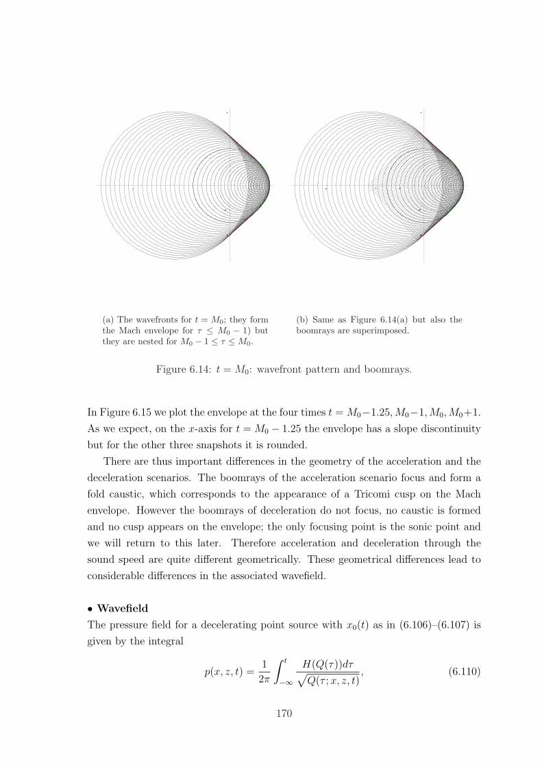
(a) The wavefronts for t = M0; they formthe Mach envelope for τ ≤ M0 − 1) butthey are nested for M0 − 1 ≤ τ ≤ M0.
(b) Same as Figure 6.14(a) but also theboomrays are superimposed.
Figure 6.14: t = M0: wavefront pattern and boomrays.
In Figure 6.15 we plot the envelope at the four times t = M0−1.25,M0−1,M0,M0+1.
As we expect, on the x-axis for t = M0 − 1.25 the envelope has a slope discontinuity
but for the other three snapshots it is rounded.
There are thus important differences in the geometry of the acceleration and the
deceleration scenarios. The boomrays of the acceleration scenario focus and form a
fold caustic, which corresponds to the appearance of a Tricomi cusp on the Mach
envelope. However the boomrays of deceleration do not focus, no caustic is formed
and no cusp appears on the envelope; the only focusing point is the sonic point and
we will return to this later. Therefore acceleration and deceleration through the
sound speed are quite different geometrically. These geometrical differences lead to
considerable differences in the associated wavefield.
• Wavefield
The pressure field for a decelerating point source with x0(t) as in (6.106)–(6.107) is
given by the integral
p(x, z, t) =1
2π
∫ t
−∞
H(Q(τ))dτ√Q(τ ;x, z, t)
, (6.110)
170
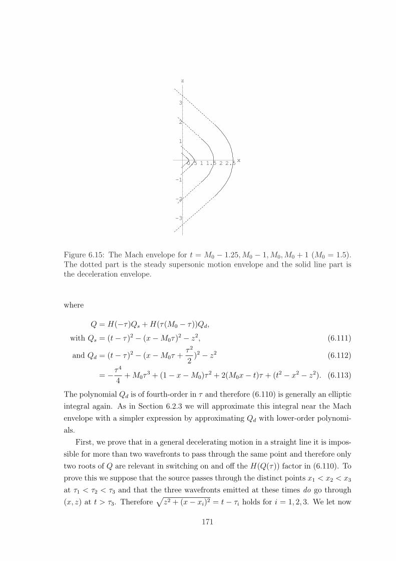
0.5 1 1.5 2 2.5x
-3
-2
-1
1
2
3
z
Figure 6.15: The Mach envelope for t = M0 − 1.25,M0 − 1,M0,M0 + 1 (M0 = 1.5).The dotted part is the steady supersonic motion envelope and the solid line part isthe deceleration envelope.
where
Q = H(−τ)Qs +H(τ(M0 − τ))Qd,
with Qs = (t− τ)2 − (x−M0τ)2 − z2, (6.111)
and Qd = (t− τ)2 − (x−M0τ +τ 2
2)2 − z2 (6.112)
= −τ4
4+M0τ
3 + (1− x−M0)τ2 + 2(M0x− t)τ + (t2 − x2 − z2). (6.113)
The polynomial Qd is of fourth-order in τ and therefore (6.110) is generally an elliptic
integral again. As in Section 6.2.3 we will approximate this integral near the Mach
envelope with a simpler expression by approximating Qd with lower-order polynomi-
als.
First, we prove that in a general decelerating motion in a straight line it is impos-
sible for more than two wavefronts to pass through the same point and therefore only
two roots of Q are relevant in switching on and off the H(Q(τ)) factor in (6.110). To
prove this we suppose that the source passes through the distinct points x1 < x2 < x3
at τ1 < τ2 < τ3 and that the three wavefronts emitted at these times do go through
(x, z) at t > τ3. Therefore√z2 + (x− xi)2 = t− τi holds for i = 1, 2, 3. We let now
171
Xi = x− xi and therefore X1 > X2 > X3. The mean source speed over [τ1, τ2] is
u12 =x2 − x1
τ2 − τ1=
X1 −X2√z2 +X2
1 −√z2 +X2
2
, (6.114)
and similarly over [τ2, τ3] the mean speed is u23. If the motion is decelerating thenu23 < u12 which can also be written as 1/u12 < 1/u23, i.e.
√z2 +X2
1 −√z2 +X2
2
X1 −X2
<
√z2 +X2
2 −√z2 +X2
3
X2 −X3
. (6.115)
However inequality (6.115) is impossible because√z2 +X2 is a convex function; the
left-hand side of (6.115) is the slope of the chord BC (see Figure 6.16) and the right-
hand side is the slope of the chord AB and for a convex function the former slope
is greater than the latter slope. Therefore not more than two wavefronts can pass
X1X2X3
AB
C
Figure 6.16: For a convex function the slope of the chord AB is less than the slopeof the chord BC.
through a point in the region of influence.7 In this case the wavefronts are exactly
two. This is because Q < 0 as τ → −∞ and at τ = t but for some τ we have Q > 0
because (x, z) is inside the region of influence; this means that Q becomes zero at
exactly two values of τ . We denote these roots by τ1 and τ2. The maximum value
of Q is attained for a τm such that τ1 < τm < τ2. If (x, z) is outside the region of
influence we have Q < 0, and the integral (6.110) is zero.
We can think of the region of influence as composed of three regions, according to
whether the two wavefronts are both from Qs, both from Qd or one from each. We
will discuss these regions with the help of Figure 6.18, where we plot Q for the five
points A, B, O, C, D shown in Figure 6.17. The first region is on the left of the IW
7For a general accelerating motion the inequality (6.115) is reversed and therefore there couldbe points in the region of influence where three wavefronts may go through. For the constantacceleration case, considered earlier, such points have indeed been identified; they were the cusps.
172
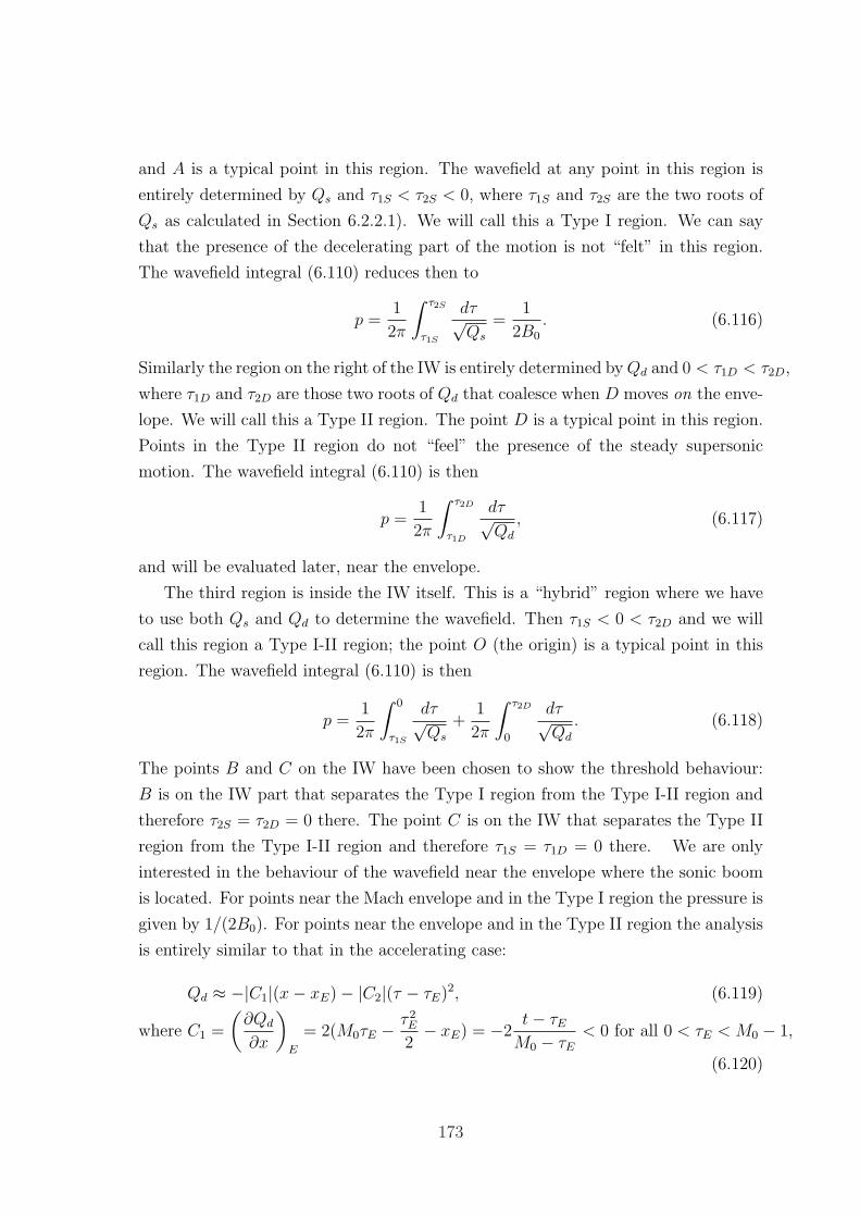
and A is a typical point in this region. The wavefield at any point in this region is
entirely determined by Qs and τ1S < τ2S < 0, where τ1S and τ2S are the two roots of
Qs as calculated in Section 6.2.2.1). We will call this a Type I region. We can say
that the presence of the decelerating part of the motion is not “felt” in this region.
The wavefield integral (6.110) reduces then to
p =1
2π
∫ τ2S
τ1S
dτ√Qs
=1
2B0
. (6.116)
Similarly the region on the right of the IW is entirely determined byQd and 0 < τ1D < τ2D,
where τ1D and τ2D are those two roots of Qd that coalesce when D moves on the enve-
lope. We will call this a Type II region. The point D is a typical point in this region.
Points in the Type II region do not “feel” the presence of the steady supersonic
motion. The wavefield integral (6.110) is then
p =1
2π
∫ τ2D
τ1D
dτ√Qd
, (6.117)
and will be evaluated later, near the envelope.
The third region is inside the IW itself. This is a “hybrid” region where we have
to use both Qs and Qd to determine the wavefield. Then τ1S < 0 < τ2D and we will
call this region a Type I-II region; the point O (the origin) is a typical point in this
region. The wavefield integral (6.110) is then
p =1
2π
∫ 0
τ1S
dτ√Qs
+1
2π
∫ τ2D
0
dτ√Qd
. (6.118)
The points B and C on the IW have been chosen to show the threshold behaviour:
B is on the IW part that separates the Type I region from the Type I-II region and
therefore τ2S = τ2D = 0 there. The point C is on the IW that separates the Type II
region from the Type I-II region and therefore τ1S = τ1D = 0 there. We are only
interested in the behaviour of the wavefield near the envelope where the sonic boom
is located. For points near the Mach envelope and in the Type I region the pressure is
given by 1/(2B0). For points near the envelope and in the Type II region the analysis
is entirely similar to that in the accelerating case:
Qd ≈ −|C1|(x− xE)− |C2|(τ − τE)2, (6.119)
where C1 =
(∂Qd
∂x
)
E
= 2(M0τE − τ 2E
2− xE) = −2
t− τEM0 − τE
< 0 for all 0 < τE < M0 − 1,
(6.120)
173
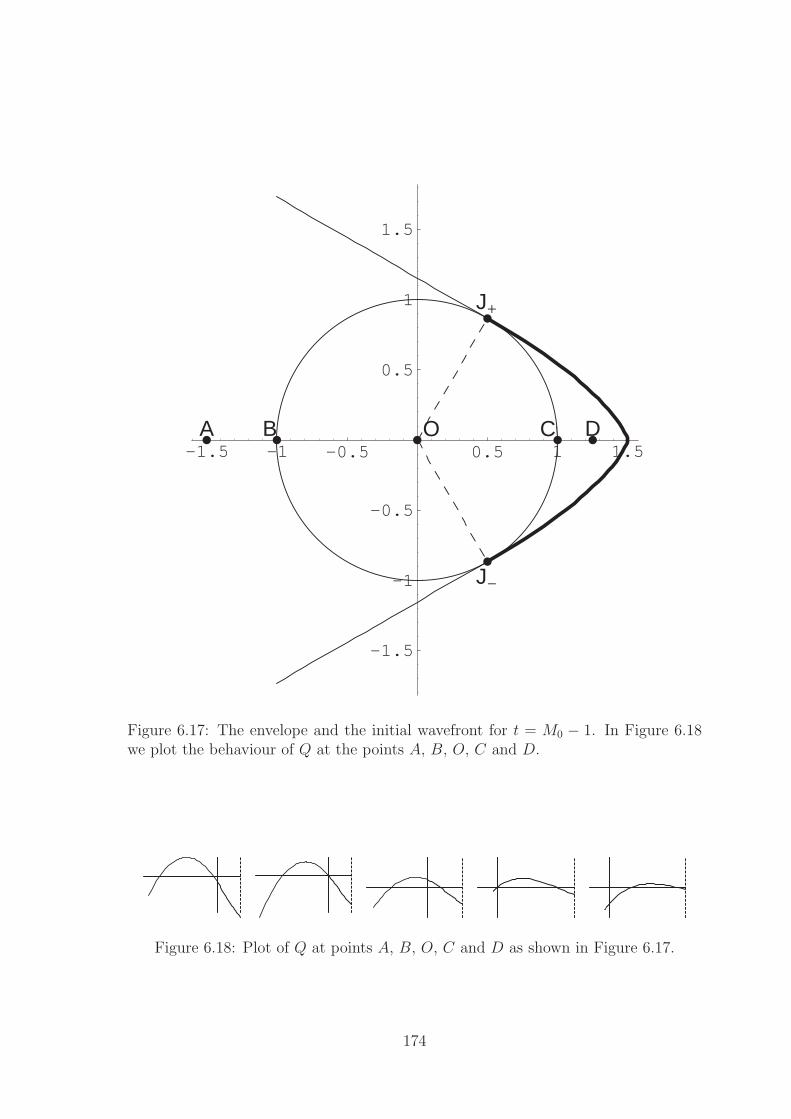
-1.5 -1 -0.5 0.5 1 1.5
-1.5
-1
-0.5
0.5
1
1.5
A B O C D
J+
J-
Figure 6.17: The envelope and the initial wavefront for t = M0 − 1. In Figure 6.18we plot the behaviour of Q at the points A, B, O, C and D.
Figure 6.18: Plot of Q at points A, B, O, C and D as shown in Figure 6.17.
174
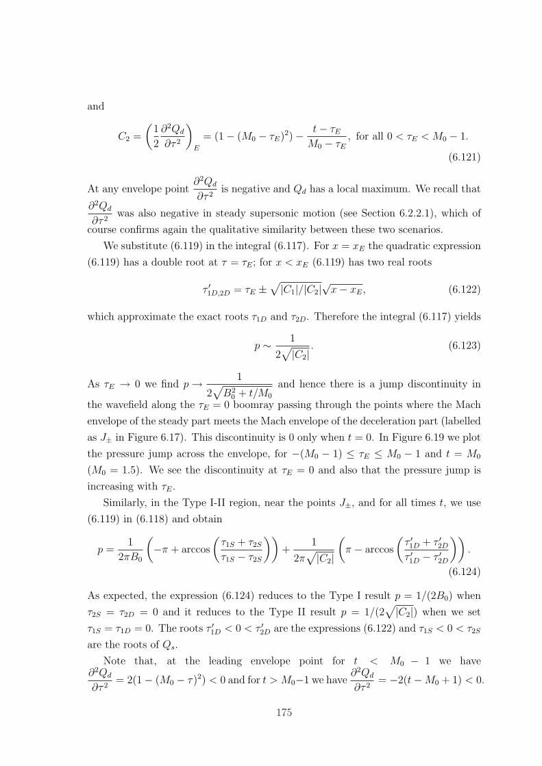
and
C2 =
(1
2
∂2Qd
∂τ 2
)
E
= (1− (M0 − τE)2)− t− τEM0 − τE
, for all 0 < τE < M0 − 1.
(6.121)
At any envelope point∂2Qd
∂τ 2is negative and Qd has a local maximum. We recall that
∂2Qd
∂τ 2was also negative in steady supersonic motion (see Section 6.2.2.1), which of
course confirms again the qualitative similarity between these two scenarios.
We substitute (6.119) in the integral (6.117). For x = xE the quadratic expression
(6.119) has a double root at τ = τE; for x < xE (6.119) has two real roots
τ ′1D,2D = τE ±√|C1|/|C2|
√x− xE, (6.122)
which approximate the exact roots τ1D and τ2D. Therefore the integral (6.117) yields
p ∼ 1
2√|C2|
. (6.123)
As τE → 0 we find p→ 1
2√B2
0 + t/M0
and hence there is a jump discontinuity in
the wavefield along the τE = 0 boomray passing through the points where the Mach
envelope of the steady part meets the Mach envelope of the deceleration part (labelled
as J± in Figure 6.17). This discontinuity is 0 only when t = 0. In Figure 6.19 we plot
the pressure jump across the envelope, for −(M0 − 1) ≤ τE ≤ M0 − 1 and t = M0
(M0 = 1.5). We see the discontinuity at τE = 0 and also that the pressure jump is
increasing with τE.
Similarly, in the Type I-II region, near the points J±, and for all times t, we use
(6.119) in (6.118) and obtain
p =1
2πB0
(−π + arccos
(τ1S + τ2Sτ1S − τ2S
))+
1
2π√|C2|
(π − arccos
(τ ′1D + τ ′2Dτ ′1D − τ ′2D
)).
(6.124)
As expected, the expression (6.124) reduces to the Type I result p = 1/(2B0) when
τ2S = τ2D = 0 and it reduces to the Type II result p = 1/(2√|C2|) when we set
τ1S = τ1D = 0. The roots τ ′1D < 0 < τ ′2D are the expressions (6.122) and τ1S < 0 < τ2S
are the roots of Qs.
Note that, at the leading envelope point for t < M0 − 1 we have∂2Qd
∂τ 2= 2(1− (M0 − τ)2) < 0 and for t > M0−1 we have
∂2Qd
∂τ 2= −2(t−M0 + 1) < 0.
175
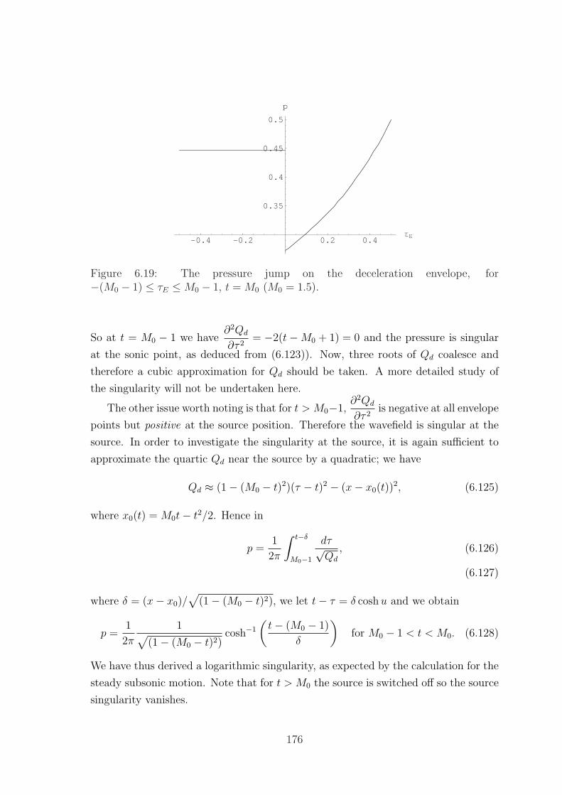
-0.4 -0.2 0.2 0.4ΤE
0.35
0.4
0.45
0.5
p
Figure 6.19: The pressure jump on the deceleration envelope, for−(M0 − 1) ≤ τE ≤M0 − 1, t = M0 (M0 = 1.5).
So at t = M0 − 1 we have∂2Qd
∂τ 2= −2(t−M0 + 1) = 0 and the pressure is singular
at the sonic point, as deduced from (6.123)). Now, three roots of Qd coalesce and
therefore a cubic approximation for Qd should be taken. A more detailed study of
the singularity will not be undertaken here.
The other issue worth noting is that for t > M0−1,∂2Qd
∂τ 2is negative at all envelope
points but positive at the source position. Therefore the wavefield is singular at the
source. In order to investigate the singularity at the source, it is again sufficient to
approximate the quartic Qd near the source by a quadratic; we have
Qd ≈ (1− (M0 − t)2)(τ − t)2 − (x− x0(t))2, (6.125)
where x0(t) = M0t− t2/2. Hence in
p =1
2π
∫ t−δ
M0−1
dτ√Qd
, (6.126)
(6.127)
where δ = (x− x0)/√
(1− (M0 − t)2), we let t− τ = δ coshu and we obtain
p =1
2π
1√(1− (M0 − t)2)
cosh−1
(t− (M0 − 1)
δ
)for M0 − 1 < t < M0. (6.128)
We have thus derived a logarithmic singularity, as expected by the calculation for the
steady subsonic motion. Note that for t > M0 the source is switched off so the source
singularity vanishes.
176
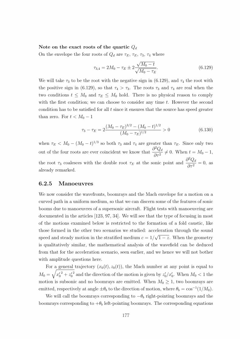
Note on the exact roots of the quartic Qd
On the envelope the four roots of Qd are τE, τE, τ3, τ4 where
τ3,4 = 2M0 − τE ± 2
√M0 − t√M0 − τE
. (6.129)
We will take τ3 to be the root with the negative sign in (6.129), and τ4 the root with
the positive sign in (6.129), so that τ4 > τ3. The roots τ3 and τ4 are real when the
two conditions t ≤ M0 and τE ≤ M0 hold. There is no physical reason to comply
with the first condition; we can choose to consider any time t. However the second
condition has to be satisfied for all t since it ensures that the source has speed greater
than zero. For t < M0 − 1
τ3 − τE = 2(M0 − τE)3/2 − (M0 − t)1/2
(M0 − τE)1/2> 0 (6.130)
when τE < M0 − (M0 − t)1/3 so both τ3 and τ4 are greater than τE. Since only two
out of the four roots are ever coincident we know that∂2Qd
∂τ 26= 0. When t = M0 − 1,
the root τ3 coalesces with the double root τE at the sonic point and∂2Qd
∂τ 2= 0, as
already remarked.
6.2.5 Manoeuvres
We now consider the wavefronts, boomrays and the Mach envelope for a motion on a
curved path in a uniform medium, so that we can discern some of the features of sonic
booms due to manoeuvres of a supersonic aircraft. Flight tests with manoeuvring are
documented in the articles [123, 97, 34]. We will see that the type of focusing in most
of the motions examined below is restricted to the formation of a fold caustic, like
those formed in the other two scenarios we studied: acceleration through the sound
speed and steady motion in the stratified medium c = 1/√
1− z. When the geometry
is qualitatively similar, the mathematical analysis of the wavefield can be deduced
from that for the acceleration scenario, seen earlier, and we hence we will not bother
with amplitude questions here.
For a general trajectory (x0(t), z0(t)), the Mach number at any point is equal to
M0 =√x′0
2 + z′02 and the direction of the motion is given by z′0/x
′0. When M0 < 1 the
motion is subsonic and no boomrays are emitted. When M0 ≥ 1, two boomrays are
emitted, respectively at angle ±θb to the direction of motion, where θb = cos−1(1/M0).
We will call the boomrays corresponding to −θb right-pointing boomrays and the
boomrays corresponding to +θb left-pointing boomrays. The corresponding equations
177
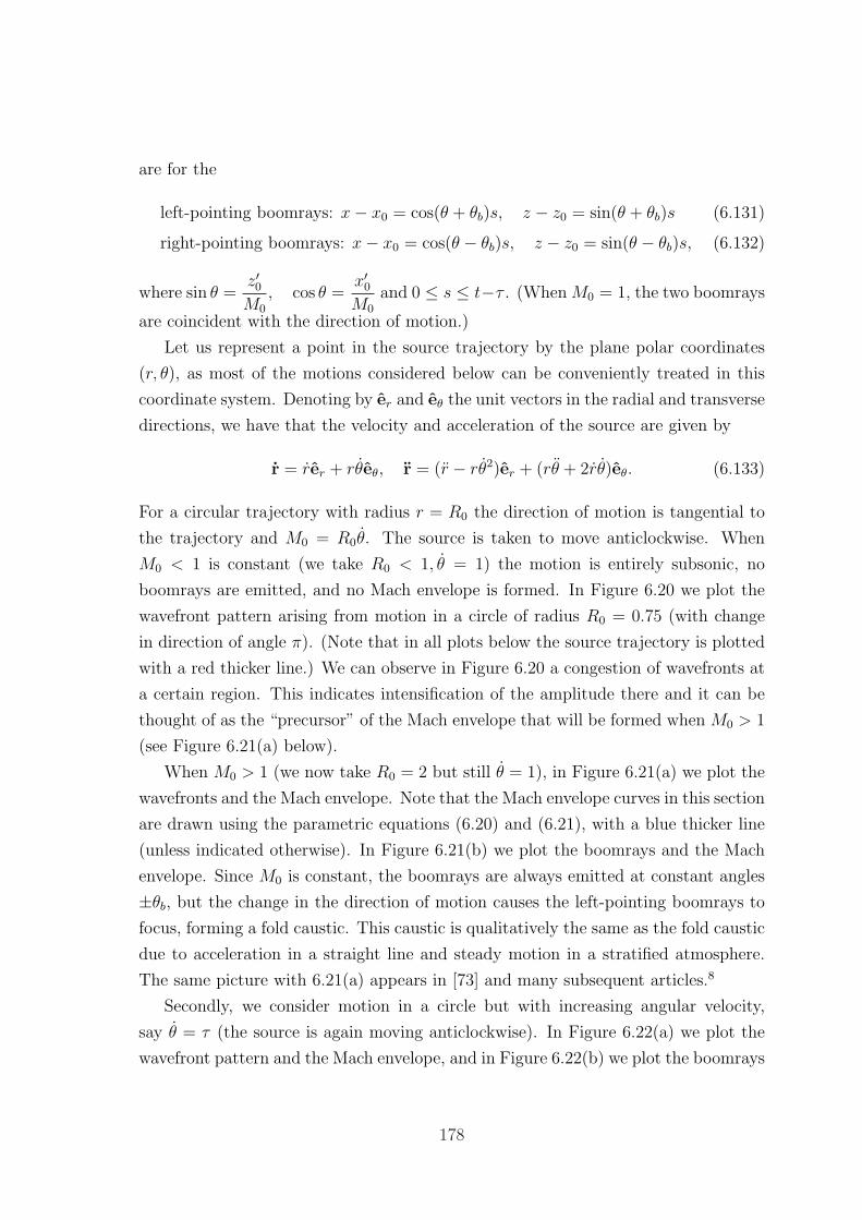
are for the
left-pointing boomrays: x− x0 = cos(θ + θb)s, z − z0 = sin(θ + θb)s (6.131)
right-pointing boomrays: x− x0 = cos(θ − θb)s, z − z0 = sin(θ − θb)s, (6.132)
where sin θ =z′0M0
, cos θ =x′0M0
and 0 ≤ s ≤ t−τ . (WhenM0 = 1, the two boomrays
are coincident with the direction of motion.)
Let us represent a point in the source trajectory by the plane polar coordinates
(r, θ), as most of the motions considered below can be conveniently treated in this
coordinate system. Denoting by er and eθ the unit vectors in the radial and transverse
directions, we have that the velocity and acceleration of the source are given by
r = rer + rθeθ, r = (r − rθ2)er + (rθ + 2rθ)eθ. (6.133)
For a circular trajectory with radius r = R0 the direction of motion is tangential to
the trajectory and M0 = R0θ. The source is taken to move anticlockwise. When
M0 < 1 is constant (we take R0 < 1, θ = 1) the motion is entirely subsonic, no
boomrays are emitted, and no Mach envelope is formed. In Figure 6.20 we plot the
wavefront pattern arising from motion in a circle of radius R0 = 0.75 (with change
in direction of angle π). (Note that in all plots below the source trajectory is plotted
with a red thicker line.) We can observe in Figure 6.20 a congestion of wavefronts at
a certain region. This indicates intensification of the amplitude there and it can be
thought of as the “precursor” of the Mach envelope that will be formed when M0 > 1
(see Figure 6.21(a) below).
When M0 > 1 (we now take R0 = 2 but still θ = 1), in Figure 6.21(a) we plot the
wavefronts and the Mach envelope. Note that the Mach envelope curves in this section
are drawn using the parametric equations (6.20) and (6.21), with a blue thicker line
(unless indicated otherwise). In Figure 6.21(b) we plot the boomrays and the Mach
envelope. Since M0 is constant, the boomrays are always emitted at constant angles
±θb, but the change in the direction of motion causes the left-pointing boomrays to
focus, forming a fold caustic. This caustic is qualitatively the same as the fold caustic
due to acceleration in a straight line and steady motion in a stratified atmosphere.
The same picture with 6.21(a) appears in [73] and many subsequent articles.8
Secondly, we consider motion in a circle but with increasing angular velocity,
say θ = τ (the source is again moving anticlockwise). In Figure 6.22(a) we plot the
wavefront pattern and the Mach envelope, and in Figure 6.22(b) we plot the boomrays
178
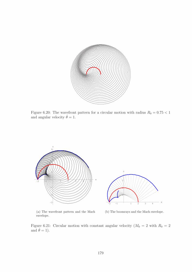
Figure 6.20: The wavefront pattern for a circular motion with radius R0 = 0.75 < 1and angular velocity θ = 1.
-2 -1 1 2 3 4 5x
-3
-2
-1
1
2
3
4z
(a) The wavefront pattern and the Machenvelope.
-2 -1 1 2 3 4x
1
2
3
z
(b) The boomrays and the Mach envelope.
Figure 6.21: Circular motion with constant angular velocity (M0 = 2 with R0 = 2and θ = 1).
179
-2 2 4x
-3
-2
-1
1
2
3
z
(a) The wavefront pattern and the Machenvelope.
-2 -1 1 2 3x
-2
-1
1
2
3
z
(b) The boomrays and the Mach envelope.
Figure 6.22: Motion in a circle with non-constant angular velocity (R0 = 2, θ = τ).
and the Mach envelope (we take 0 ≤ τ ≤ π). We see from Figure 6.22(b) that now
also the right-pointing boomrays form a fold caustic. The Mach envelope is now a
closed curve featuring two Tricomi cusps, and it looks like a distorted version of the
envelope of the accelerating motion in a straight line.
Thirdly, we consider a motion on the parabolic trajectory x0(t) = t, z0(t) = −t2.This motion is an example for a motion that decelerates and then accelerates. The
Mach number is M0 =√
1 + 4t2. For t < 0 the source moves supersonically while
decelerating, at t = 0 it touches the sound speed and for t > 0 it accelerates.
In Figure 6.23(a) we plot the wavefront pattern and the Mach envelope for for
t = 1 and launch times −1 ≤ τ ≤ t = 1. In Figure 6.23(b) we plot the boomrays and
the Mach envelope. The boomray pattern has now some additional features. One of
the two boomrays is always in the x-direction because x0 = 1 = sound speed. When
−1 < τ < 0 (deceleration) the boomrays trace the light blue part of the envelope. The
horizontal boomrays in this case are right-pointing. At time τ = 0, the two boomrays
are emitted from the origin and coincide, giving the sonic point of the envelope. The
tangent to the envelope at this sonic point is normal to the x-axis. Subsequently, for
0 < τ ≤ 1 the horizontal left-pointing boomrays from the acceleration phase trace
again the part of the light blue envelope in z ≤ 0. Therefore the x > 0, z < 0 region
8We have not seen the plot of Figure 6.20 somewhere though.
180
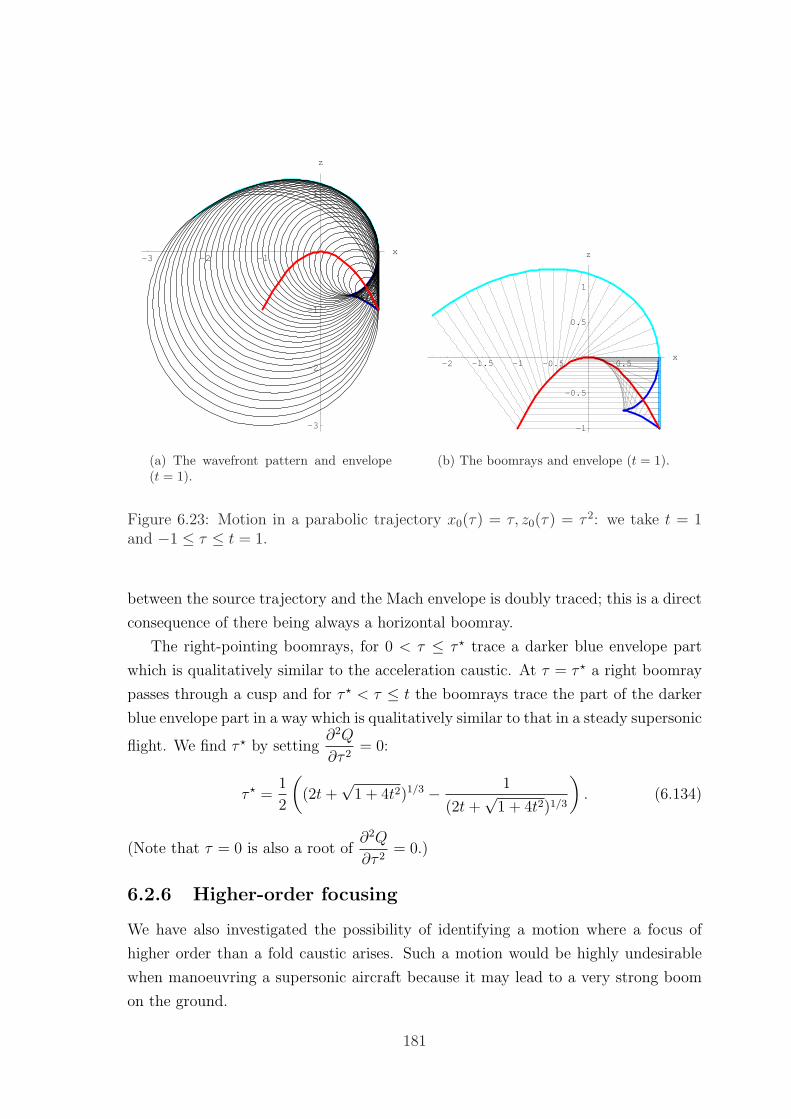
-3 -2 -1 1x
-3
-2
-1
1
z
(a) The wavefront pattern and envelope(t = 1).
-2 -1.5 -1 -0.5 0.5 1x
-1
-0.5
0.5
1
z
(b) The boomrays and envelope (t = 1).
Figure 6.23: Motion in a parabolic trajectory x0(τ) = τ, z0(τ) = τ 2: we take t = 1and −1 ≤ τ ≤ t = 1.
between the source trajectory and the Mach envelope is doubly traced; this is a direct
consequence of there being always a horizontal boomray.
The right-pointing boomrays, for 0 < τ ≤ τ ? trace a darker blue envelope part
which is qualitatively similar to the acceleration caustic. At τ = τ ? a right boomray
passes through a cusp and for τ ? < τ ≤ t the boomrays trace the part of the darker
blue envelope part in a way which is qualitatively similar to that in a steady supersonic
flight. We find τ ? by setting∂2Q
∂τ 2= 0:
τ ? =1
2
((2t+
√1 + 4t2)1/3 − 1
(2t+√
1 + 4t2)1/3
). (6.134)
(Note that τ = 0 is also a root of∂2Q
∂τ 2= 0.)
6.2.6 Higher-order focusing
We have also investigated the possibility of identifying a motion where a focus of
higher order than a fold caustic arises. Such a motion would be highly undesirable
when manoeuvring a supersonic aircraft because it may lead to a very strong boom
on the ground.
181
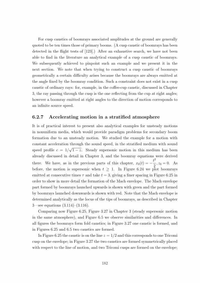
For cusp caustics of boomrays associated amplitudes at the ground are generally
quoted to be ten times those of primary booms. (A cusp caustic of boomrays has been
detected in the flight tests of [123].) After an exhaustive search, we have not been
able to find in the literature an analytical example of a cusp caustic of boomrays.
We subsequently achieved to pinpoint such an example and we present it in the
next section. We note that when trying to construct a cusp caustic of boomrays
geometrically a certain difficulty arises because the boomrays are always emitted at
the angle fixed by the boomray condition. Such a constraint does not exist in a cusp
caustic of ordinary rays: for, example, in the coffee-cup caustic, discussed in Chapter
3, the ray passing through the cusp is the one reflecting from the cup at right angles;
however a boomray emitted at right angles to the direction of motion corresponds to
an infinite source speed.
6.2.7 Accelerating motion in a stratified atmosphere
It is of practical interest to present also analytical examples for unsteady motions
in nonuniform media, which would provide paradigm problems for secondary boom
formation due to an unsteady motion. We studied the example for a motion with
constant acceleration through the sound speed, in the stratified medium with sound
speed profile c = 1/√
1− z. Steady supersonic motion in this medium has been
already discussed in detail in Chapter 3, and the boomray equations were derived
there. We have, as in the previous parts of this chapter, x0(t) = −t2
2, z0 = 0. As
before, the motion is supersonic when t ≥ 1. In Figure 6.24 we plot boomrays
emitted at consecutive times τ and take t = 3, giving a finer spacing in Figure 6.25 in
order to show in more detail the formation of the Mach envelope. The Mach envelope
part formed by boomrays launched upwards is shown with green and the part formed
by boomrays launched downwards is shown with red. Note that the Mach envelope is
determined analytically as the locus of the tips of boomrays, as described in Chapter
3—see equations (3.114)–(3.116).
Comparing now Figure 6.25, Figure 3.27 in Chapter 3 (steady supersonic motion
in the same atmosphere), and Figure 6.5 we observe similarities and differences. In
all figures the boomrays form fold caustics; in Figure 3.27 one caustic is formed, and
in Figures 6.25 and 6.5 two caustics are formed.
In Figure 6.25 the caustic is on the line z = 1/2 and this corresponds to one Tricomi
cusp on the envelope; in Figure 3.27 the two caustics are formed symmetrically placed
with respect to the line of motion, and two Tricomi cusps are formed on the envelope;
182
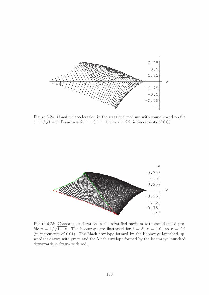
-4 -3 -2 -1x
-1
-0.75
-0.5
-0.25
0.25
0.5
0.75
z
Figure 6.24: Constant acceleration in the stratified medium with sound speed profilec = 1/
√1− z: Boomrays for t = 3, τ = 1.1 to τ = 2.9, in increments of 0.05.
-4 -3 -2 -1x
-1-0.75-0.5-0.25
0.250.50.75
z
Figure 6.25: Constant acceleration in the stratified medium with sound speed pro-file c = 1/
√1− z. The boomrays are ilustrated for t = 3, τ = 1.01 to τ = 2.9
(in increments of 0.01). The Mach envelope formed by the boomrays launched up-wards is drawn with green and the Mach envelope formed by the boomrays launcheddownwards is drawn with red.
183
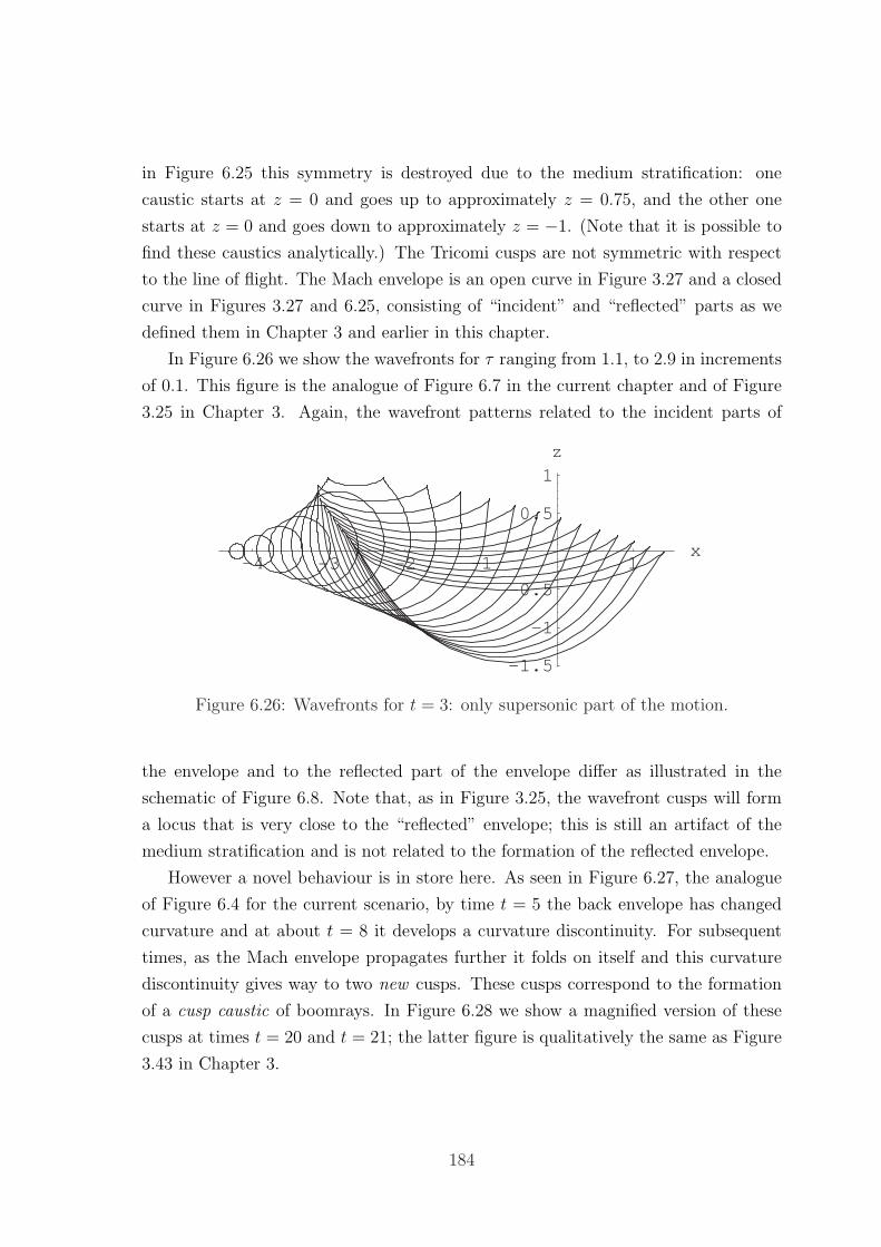
in Figure 6.25 this symmetry is destroyed due to the medium stratification: one
caustic starts at z = 0 and goes up to approximately z = 0.75, and the other one
starts at z = 0 and goes down to approximately z = −1. (Note that it is possible to
find these caustics analytically.) The Tricomi cusps are not symmetric with respect
to the line of flight. The Mach envelope is an open curve in Figure 3.27 and a closed
curve in Figures 3.27 and 6.25, consisting of “incident” and “reflected” parts as we
defined them in Chapter 3 and earlier in this chapter.
In Figure 6.26 we show the wavefronts for τ ranging from 1.1, to 2.9 in increments
of 0.1. This figure is the analogue of Figure 6.7 in the current chapter and of Figure
3.25 in Chapter 3. Again, the wavefront patterns related to the incident parts of
-4 -3 -2 -1 1x
-1.5
-1
-0.5
0.5
1z
Figure 6.26: Wavefronts for t = 3: only supersonic part of the motion.
the envelope and to the reflected part of the envelope differ as illustrated in the
schematic of Figure 6.8. Note that, as in Figure 3.25, the wavefront cusps will form
a locus that is very close to the “reflected” envelope; this is still an artifact of the
medium stratification and is not related to the formation of the reflected envelope.
However a novel behaviour is in store here. As seen in Figure 6.27, the analogue
of Figure 6.4 for the current scenario, by time t = 5 the back envelope has changed
curvature and at about t = 8 it develops a curvature discontinuity. For subsequent
times, as the Mach envelope propagates further it folds on itself and this curvature
discontinuity gives way to two new cusps. These cusps correspond to the formation
of a cusp caustic of boomrays. In Figure 6.28 we show a magnified version of these
cusps at times t = 20 and t = 21; the latter figure is qualitatively the same as Figure
3.43 in Chapter 3.
184
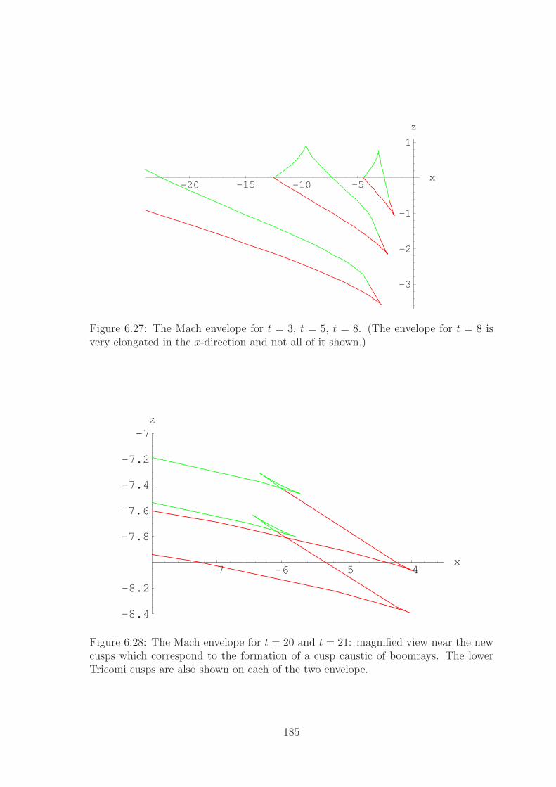
-20 -15 -10 -5x
-3
-2
-1
1
z
Figure 6.27: The Mach envelope for t = 3, t = 5, t = 8. (The envelope for t = 8 isvery elongated in the x-direction and not all of it shown.)
-7 -6 -5 -4x
-8.4
-8.2
-7.8
-7.6
-7.4
-7.2
-7z
Figure 6.28: The Mach envelope for t = 20 and t = 21: magnified view near the newcusps which correspond to the formation of a cusp caustic of boomrays. The lowerTricomi cusps are also shown on each of the two envelope.
185
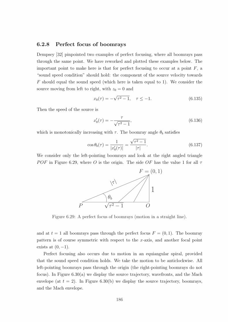
6.2.8 Perfect focus of boomrays
Dempsey [32] pinpointed two examples of perfect focusing, where all boomrays pass
through the same point. We have reworked and plotted these examples below. The
important point to make here is that for perfect focusing to occur at a point F , a
“sound speed condition” should hold: the component of the source velocity towards
F should equal the sound speed (which here is taken equal to 1). We consider the
source moving from left to right, with z0 = 0 and
x0(τ) = −√τ 2 − 1, τ ≤ −1. (6.135)
Then the speed of the source is
x′0(τ) = − τ√τ 2 − 1
, (6.136)
which is monotonically increasing with τ . The boomray angle θb satisfies
cos θb(τ) =1
|x′0(τ)|=
√τ 2 − 1
|τ | . (6.137)
We consider only the left-pointing boomrays and look at the right angled triangle
POF in Figure 6.29, where O is the origin. The side OF has the value 1 for all τ
θb
P
1
√τ 2 − 1 O
F = (0, 1)
|τ |
Figure 6.29: A perfect focus of boomrays (motion in a straight line).
and at t = 1 all boomrays pass through the perfect focus F = (0, 1). The boomray
pattern is of course symmetric with respect to the x-axis, and another focal point
exists at (0,−1).
Perfect focusing also occurs due to motion in an equiangular spiral, provided
that the sound speed condition holds. We take the motion to be anticlockwise. All
left-pointing boomrays pass through the origin (the right-pointing boomrays do not
focus). In Figure 6.30(a) we display the source trajectory, wavefronts, and the Mach
envelope (at t = 2). In Figure 6.30(b) we display the source trajectory, boomrays,
and the Mach envelope.
186
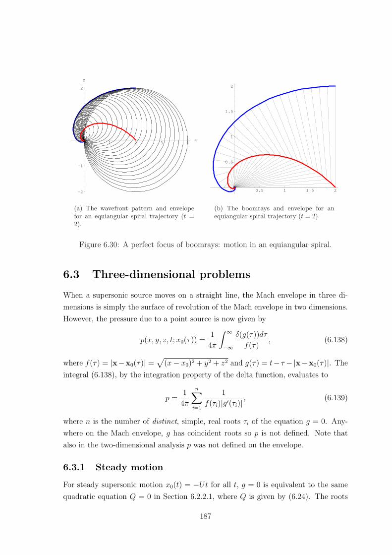
1 2 3 4x
-2
-1
1
2
z
(a) The wavefront pattern and envelopefor an equiangular spiral trajectory (t =2).
0.5 1 1.5 2
0.5
1
1.5
2
(b) The boomrays and envelope for anequiangular spiral trajectory (t = 2).
Figure 6.30: A perfect focus of boomrays: motion in an equiangular spiral.
6.3 Three-dimensional problems
When a supersonic source moves on a straight line, the Mach envelope in three di-
mensions is simply the surface of revolution of the Mach envelope in two dimensions.
However, the pressure due to a point source is now given by
p(x, y, z, t;x0(τ)) =1
4π
∫ ∞
−∞
δ(g(τ))dτ
f(τ), (6.138)
where f(τ) = |x−x0(τ)| =√
(x− x0)2 + y2 + z2 and g(τ) = t− τ −|x−x0(τ)|. The
integral (6.138), by the integration property of the delta function, evaluates to
p =1
4π
n∑i=1
1
f(τi)|g′(τi)| , (6.139)
where n is the number of distinct, simple, real roots τi of the equation g = 0. Any-
where on the Mach envelope, g has coincident roots so p is not defined. Note that
also in the two-dimensional analysis p was not defined on the envelope.
6.3.1 Steady motion
For steady supersonic motion x0(t) = −Ut for all t, g = 0 is equivalent to the same
quadratic equation Q = 0 in Section 6.2.2.1, where Q is given by (6.24). The roots
187
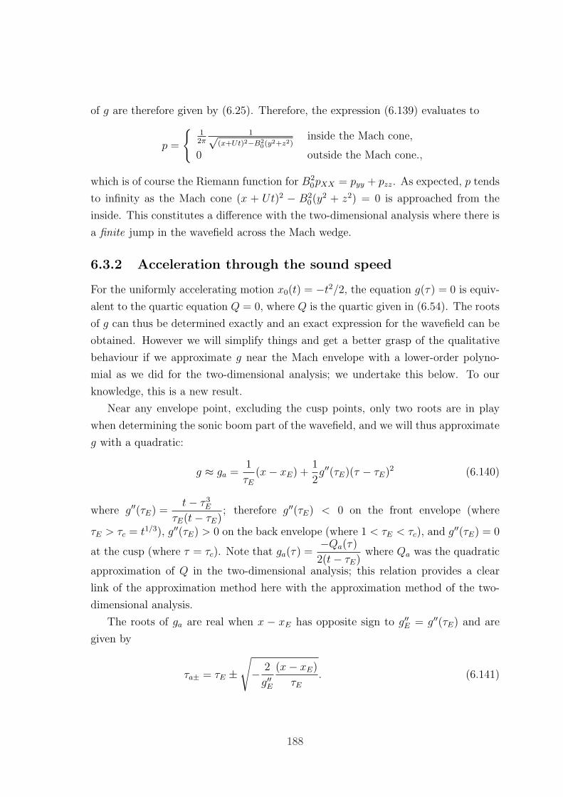
of g are therefore given by (6.25). Therefore, the expression (6.139) evaluates to
p =
{12π
1√(x+Ut)2−B2
0(y2+z2)inside the Mach cone,
0 outside the Mach cone.,
which is of course the Riemann function for B20pXX = pyy + pzz. As expected, p tends
to infinity as the Mach cone (x + Ut)2 − B20(y
2 + z2) = 0 is approached from the
inside. This constitutes a difference with the two-dimensional analysis where there is
a finite jump in the wavefield across the Mach wedge.
6.3.2 Acceleration through the sound speed
For the uniformly accelerating motion x0(t) = −t2/2, the equation g(τ) = 0 is equiv-
alent to the quartic equation Q = 0, where Q is the quartic given in (6.54). The roots
of g can thus be determined exactly and an exact expression for the wavefield can be
obtained. However we will simplify things and get a better grasp of the qualitative
behaviour if we approximate g near the Mach envelope with a lower-order polyno-
mial as we did for the two-dimensional analysis; we undertake this below. To our
knowledge, this is a new result.
Near any envelope point, excluding the cusp points, only two roots are in play
when determining the sonic boom part of the wavefield, and we will thus approximate
g with a quadratic:
g ≈ ga =1
τE(x− xE) +
1
2g′′(τE)(τ − τE)2 (6.140)
where g′′(τE) =t− τ 3
E
τE(t− τE); therefore g′′(τE) < 0 on the front envelope (where
τE > τc = t1/3), g′′(τE) > 0 on the back envelope (where 1 < τE < τc), and g′′(τE) = 0
at the cusp (where τ = τc). Note that ga(τ) =−Qa(τ)
2(t− τE)where Qa was the quadratic
approximation of Q in the two-dimensional analysis; this relation provides a clear
link of the approximation method here with the approximation method of the two-
dimensional analysis.
The roots of ga are real when x − xE has opposite sign to g′′E = g′′(τE) and are
given by
τa± = τE ±√− 2
g′′E
(x− xE)
τE. (6.141)
188
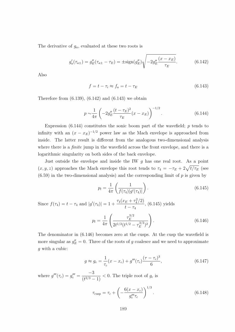
The derivative of ga, evaluated at these two roots is
g′a(τa±) = g′′E(τa± − τE) = ±sign(g′′E)
√−2g′′E
(x− xE)
τE. (6.142)
Also
f = t− τi ≈ fa = t− τE (6.143)
Therefore from (6.139), (6.142) and (6.143) we obtain
p ∼ 1
4π
(−2g′′E
(t− τE)2
τE(x− xE)
)−1/2
. (6.144)
Expression (6.144) constitutes the sonic boom part of the wavefield; p tends to
infinity with an (x − xE)−1/2 power law as the Mach envelope is approached from
inside. The latter result is different from the analogous two-dimensional analysis
where there is a finite jump in the wavefield across the front envelope, and there is a
logarithmic singularity on both sides of the back envelope.
Just outside the envelope and inside the IW g has one real root. As a point
(x, y, z) approaches the Mach envelope this root tends to τ4 = −τE + 2√t/τE (see
(6.59) in the two-dimensional analysis) and the corresponding limit of p is given by
pl =1
4π
(1
f(τ4)|g′(τ4)|). (6.145)
Since f(τ4) = t− τ4 and |g′(τ4)| = 1 +τ4(xE + τ 2
4 /2)
t− τ4, (6.145) yields
pl =1
4π
(τ
3/2E
2t1/2(t1/2 − τ3/2E )2
). (6.146)
The denominator in (6.146) becomes zero at the cusps. At the cusp the wavefield is
more singular as g′′E = 0. Three of the roots of g coalesce and we need to approximate
g with a cubic:
g ≈ gc =1
τc(x− xc) + g′′′(τc)
(τ − τc)3
6, (6.147)
where g′′′(τc) = g′′′c =−3
(t2/3 − 1)< 0. The triple root of gc is
τcusp = τc +
(−6(x− xc)
g′′′c τc
)1/3
. (6.148)
189
Therefore on either side of the cusp, at leading order, p is given by
pc ∼ 1
2π
6−2/3τ2/3c
(t− τc)|g′′′c |1/3|x− xc|−2/3. (6.149)
From (6.149) we conclude that at the cusp p goes to infinity with the power law
|x− xc|−2/3.
We close this section by plotting the trace of the fold caustic with a horizontal
plane, which models the ground. The fold caustic is the surface
y2c + z2
c = −(
2
3xc +
1
3
)3
, (6.150)
obtained by revolution of (6.47) around the x-axis. The intersection of (6.150) with
the ground, which is represented here by z = zg, is thus
y2c = −
(2
3xc +
1
3
)3
− z2g . (6.151)
It is on this curve that the boom is loudest. In Figure 6.31 we plot (6.151), taking
zg = −8. We also plot the (x, y)-cut of (6.151) at the horizontal plane of motion
(dashed line). This curve is what we had arrowed as the “caustic” in Figure 1.3.
-10-8-6-4-2 x
-15
-10
-5
5
10
15
y
Figure 6.31: The trace of the fold caustic at the ground. The (x, y)-cut of the foldcaustic at the height of the source (z = 0) is also plotted (with a dashed line).
190
6.4 The link between Chapter 6 and Chapter 7
In this chapter when we evaluated the wavefield near the Mach envelope for constant-
acceleration motions in two and three dimensions we identified singularities that were
incompatible with the small-amplitude assumption of linear theory. However, solving
corresponding nonlinear problems is a formidable task. Therefore in the next chapter
we will solve a simpler one-dimensional nonlinear problem. This will be itself a
demanding task and will reveal an unexpectedly rich structure. We will see that
nonlinearities, however small they may be, regularise the sonic singularities.
191
Chapter 7
Solution of the Kinematic WaveEquation with an acceleratingpoint source
7.1 Introduction
In this chapter we solve, mainly analytically, the inhomogeneous Kinematic Wave
Equation
ut +
(u2
2
)
x
= Aδ
(x− t2
2
), with the initial condition u(x, 0) = 1, (7.1)
where A is any real number. Here, δ stands for the Dirac delta function and the
equation is interpreted in the sense of distributions. Letting u = 1 + Av we obtain
the equivalent form
vt + (1 + Av)vx = δ
(x− t2
2
), with the initial condition v(x, 0) = 0. (7.2)
This is a model equation for the interaction of nonlinearity with a point force that
accelerates through the sound speed. The point force is represented here by the
singular source term δ(x − t2/2) and the sound speed by the initial value u = 1 in
(7.1), or by the undisturbed characteristic speed 1 in (7.2). The displacement of the
source is x(t) = t2/2 (uniform acceleration) and therefore its velocity at time t is
x(t) = t. Consequently, for 0 < t < 1 the source is subsonic, it passes through a sonic
point at t = 1, and it is supersonic for t > 1.
Problem (7.1) is interesting because it constitutes an analytically tractable paradigm
for the inclusion of nonlinearities in higher-order problems that involve accelerating
motion, such as the rocket propulsion of carriages with the aim of achieving a certain
192
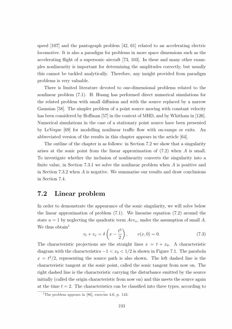
speed [107] and the pantograph problem [42, 61] related to an accelerating electric
locomotive. It is also a paradigm for problems in more space dimensions such as the
accelerating flight of a supersonic aircraft [73, 103]. In these and many other exam-
ples nonlinearity is important for determining the amplitudes correctly, but usually
this cannot be tackled analytically. Therefore, any insight provided from paradigm
problems is very valuable.
There is limited literature devoted to one-dimensional problems related to the
nonlinear problem (7.1). H. Huang has performed direct numerical simulations for
the related problem with small diffusion and with the source replaced by a narrow
Gaussian [58]. The simpler problem of a point source moving with constant velocity
has been considered by Hoffman [57] in the context of MHD, and by Whitham in [126].
Numerical simulations in the case of a stationary point source have been presented
by LeVeque [69] for modelling nonlinear traffic flow with on-ramps or exits. An
abbreviated version of the results in this chapter appears in the article [64].
The outline of the chapter is as follows: in Section 7.2 we show that a singularity
arises at the sonic point from the linear approximation of (7.2) when A is small.
To investigate whether the inclusion of nonlinearity converts the singularity into a
finite value, in Section 7.3.1 we solve the nonlinear problem when A is positive and
in Section 7.3.2 when A is negative. We summarise our results and draw conclusions
in Section 7.4.
7.2 Linear problem
In order to demonstrate the appearance of the sonic singularity, we will solve below
the linear approximation of problem (7.1). We linearise equation (7.2) around the
state u = 1 by neglecting the quadratic term Avvx, under the assumption of small A.
We thus obtain1
vt + vx = δ
(x− t2
2
), v(x, 0) = 0. (7.3)
The characteristic projections are the straight lines x = t + x0. A characteristic
diagram with the characteristics −1 < x0 < 1/2 is shown in Figure 7.1. The parabola
x = t2/2, representing the source path is also shown. The left dashed line is the
characteristic tangent at the sonic point, called the sonic tangent from now on. The
right dashed line is the characteristic carrying the disturbance emitted by the source
initially (called the origin characteristic from now on) and this meets the source again
at the time t = 2. The characteristics can be classified into three types, according to
1The problem appears in [86], exercise 4.6, p. 143.
193
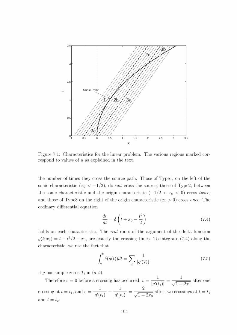
−1 −0.5 0 0.5 1 1.5 2 2.5 3 3.50
0.5
1
1.5
2
2.5
x
t
2a
1 2b
2c3b
3a
Sonic Point
Figure 7.1: Characteristics for the linear problem. The various regions marked cor-respond to values of u as explained in the text.
the number of times they cross the source path. Those of Type1, on the left of the
sonic characteristic (x0 < −1/2), do not cross the source; those of Type2, between
the sonic characteristic and the origin characteristic (−1/2 < x0 < 0) cross twice,
and those of Type3 on the right of the origin characteristic (x0 > 0) cross once. The
ordinary differential equation
dv
dt= δ
(t+ x0 − t2
2
)(7.4)
holds on each characteristic. The real roots of the argument of the delta function
g(t; x0) = t − t2/2 + x0, are exactly the crossing times. To integrate (7.4) along the
characteristic, we use the fact that
∫ b
a
δ(g(t))dt =∑i
1
|g′(Ti)| (7.5)
if g has simple zeros Ti in (a, b).
Therefore v = 0 before a crossing has occurred, v =1
|g′(t1)| =1√
1 + 2x0
after one
crossing at t = t1, and v =1
|g′(t1)| +1
|g′(t2)| =2√
1 + 2x0
after two crossings at t = t1
and t = t2.
194
Therefore v = 0 in the regions 1, 2a and 3a, v = v(x, t) =1√
1 + 2(x− t)in
regions 2b and 3b and v = v(x, t) =2√
1 + 2(x− t)in region 2c.
When t < 1 the jump in v at the source is1
1− t. This jump becomes infinite
at the sonic point (arrowed in Figure 7.1). After the sonic point, an infinite jump
continues on the sonic tangent x = t−1/2 and a finite jump continues with the source
and has value1
t− 1. A jump of fixed value 1 propagates along the characteristic x = t
undisturbed from the origin to infinity.
We have presented the exact solution of the linearised problem and deduced that
a sonic singularity emerges. Such a singularity violates the assumption of small
disturbances tied to the linear problem. We will solve below the nonlinear problem
(7.1), and show that nonlinearity converts the sonic singularity into a finite value.
7.3 Nonlinear problem
Returning to the problem (7.1), the characteristic projections have velocity dx/dt = u.
Since the variation of u along the characteristics is governed by
du
dt= Aδ(x− t2/2), (7.6)
u is constant along characteristics except for jumps when crossing the source. There-
fore before the characteristics cross the source, they are still the straight lines x =
t + x0. We still classify the characteristics by Type1, Type2 and Type3 before they
cross the source. Type1 characteristics never cross the source as in the linear problem.
If a Type2 characteristic crosses the source at time τ , u will change to a new value
we call u2R(τ), and the new characteristic, called Type2R, is
x =τ 2
2+ u(t− τ). (7.7)
We shall show below that for any characteristic crossing the source from left to right
at time τ , the relation between uL and uR, is
uR = τ +√
(uL − τ)2 + 2A. (7.8)
Therefore, applying (7.8) to the Type2R characteristics we find that
u2R = τ +√
(1− τ)2 + 2A (7.9)
195
Finally Type3 characteristics always cross the source. After crossing, they are called
Type3L and their velocity is u3L = τ −√
(1− τ)2 − 2A, found according to the
general relation
uL = τ −√
(uR − τ)2 − 2A, (7.10)
satisfied by any characteristic crossing the source from right to left at time τ . We
now derive (7.8) and (7.10). Let us define the new variable
ξ = x− t2/2 (7.11)
so that, in the (ξ, t)-plane, the source path transforms to the straight line ξ = 0 and
the characteristics have velocity
ξ = x− t = u− t with u varying on them as u = Aδ(ξ). (7.12)
Differentiating ξ with respect to t, we obtain
ξ = u− 1 = Aδ(ξ)− 1. (7.13)
Multiplying (7.13) by ξ, integrating over t, and applying the initial conditions, we
haveξ2
2= A(H(ξ)−H(x0))− ξ + x0 + 1/2 (7.14)
If a characteristic crosses the source, then applying (7.14) just on the left of the source
(ξ = 0−) and just on the right (ξ = 0+), and taking the difference, we obtain
ξ2R
2− ξ2
L
2= A (7.15)
and using (7.12) we rewrite (7.15) as
(uR − t)2 − (uL − t)2 = 2A, (7.16)
where t is the crossing time. This can also be obtained by a Rankine-Hugoniot type
argument using the conservation law (7.1). We therefore have
uR = t±√
(uL − t)2 + 2A and uL = t±√
(uR − t)2 − 2A. (7.17)
For characteristics crossing the source from left to right the velocity both on the
left and on the right is larger than the source velocity. To satisfy this we must select
the positive roots in (7.17). The first one of these equations is precisely relation (7.8),
where t = τ . However, for characteristics crossing the source from right to left the
velocity at both sides is smaller than the source velocity. Therefore in (7.17) we have
196

to pick instead the negative roots and the second equation is precisely (7.10), where
t = τ .
We finally note that relation (7.10) is also to be applied if the Type2R char-
acteristics cross the source from right to left; they would then be called Type2RL
characteristics.
As we expect from (7.6), if A > 0 the characteristics become faster on crossing the
source, but if A < 0 they become slower. We also deduce from the above discussion
that whereas all Type2 characteristics cross the source for any A > 0, for negative A
only characteristics with τ < τm = 1−√
2|A| cross, since u2R becomes complex if τm
is exceeded. These first differences between the A > 0 and A < 0 cases indicate that
the respective solutions will differ significantly. Therefore we first develop the case
A > 0 in Section 7.3.1 and later the case A < 0 in Section 7.3.2.
7.3.1 Positive force (A > 0)
In addition to the characteristic families of Type 1, 2 and 3 (and the deflected families
Type3L, Type2R and Type2RL), another family of characteristics appears in the
nonlinear problem for A > 0. These characteristics all start from x0 = −1/2, reach
the source at t = 1 and then travel for some time along the source2. If they emerge
out on the left where ξ = 0−, and at time τ ≥ 1, then (7.14) implies ξ = 0, i.e.
u = u4(τ) = τ , i.e. the characteristics emerge tangent to the source. We will call
these characteristics Type4. If they emerge on the right, where ξ = 0+, then (7.14)
implies ξ = u− τ = ±√2A and since u > τ we have u = u4R(τ) = τ +√
2A and the
characteristics emerge at an angle to the source. We will call the latter characteristics
Type4R.
Type2R and Type4R characteristics become faster as τ increases and each family,
if not prohibited, would focus into an envelope in a finite time. The solution would
become multi-valued beyond the envelopes and therefore the envelopes’ formation has
to be prevented by the introduction of shocks as we elaborate below. As an example,
we show the focusing of the Type2R family (for A = 1) in Figure 7.2.
¦ Shock from the origin
Since the Type2R characteristics are faster than Type3, these families intersect and a
multi-valued region is formed which is resolved by the introduction of a shock starting
at the origin. We will call this ShockI from now on. We shall parametrise the path
2these characteristics will therefore fill what initially appears as an empty region between thesonic tangent and the τ = 1 characteristic which has velocity u2R(τ = 1) = 1 +
√2A
197
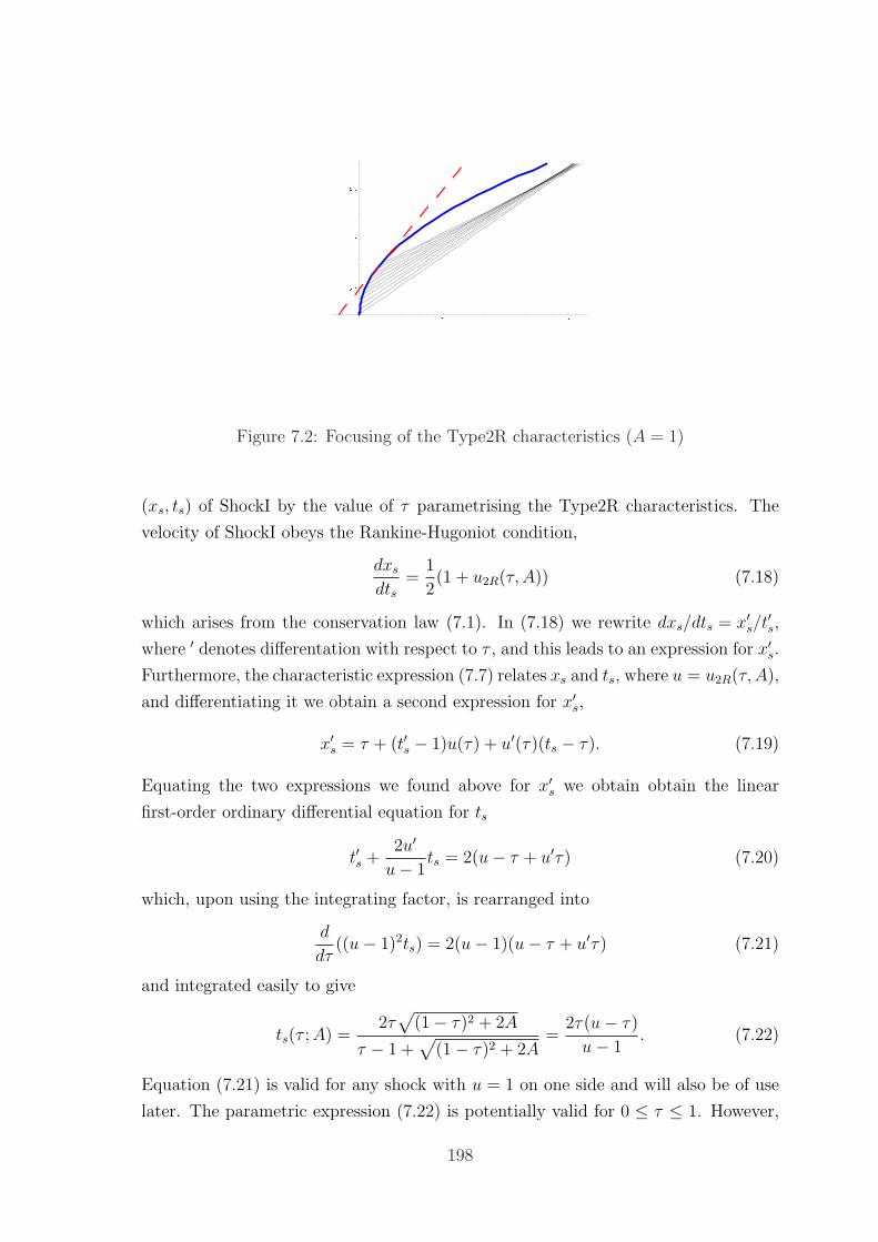
Figure 7.2: Focusing of the Type2R characteristics (A = 1)
(xs, ts) of ShockI by the value of τ parametrising the Type2R characteristics. The
velocity of ShockI obeys the Rankine-Hugoniot condition,
dxsdts
=1
2(1 + u2R(τ, A)) (7.18)
which arises from the conservation law (7.1). In (7.18) we rewrite dxs/dts = x′s/t′s,
where ′ denotes differentation with respect to τ , and this leads to an expression for x′s.
Furthermore, the characteristic expression (7.7) relates xs and ts, where u = u2R(τ, A),
and differentiating it we obtain a second expression for x′s,
x′s = τ + (t′s − 1)u(τ) + u′(τ)(ts − τ). (7.19)
Equating the two expressions we found above for x′s we obtain obtain the linear
first-order ordinary differential equation for ts
t′s +2u′
u− 1ts = 2(u− τ + u′τ) (7.20)
which, upon using the integrating factor, is rearranged into
d
dτ((u− 1)2ts) = 2(u− 1)(u− τ + u′τ) (7.21)
and integrated easily to give
ts(τ ;A) =2τ
√(1− τ)2 + 2A
τ − 1 +√
(1− τ)2 + 2A=
2τ(u− τ)
u− 1. (7.22)
Equation (7.21) is valid for any shock with u = 1 on one side and will also be of use
later. The parametric expression (7.22) is potentially valid for 0 ≤ τ ≤ 1. However,
198
it may cease to be valid when ShockI hits the source or an envelope attempts to form
on ShockI. We examine these two possibilities and we find that the first is realised
for 0 < A < 0.27551 and the second for 0.27551 < A < 1/2. We will label with
τSI the characteristic entering ShockI on the source; τSI is determined by solving
algebraically the equation xs = t2s/2. (This leads to a quartic in τ and care must be
applied to select the root that is real and less than 1.) The point on ShockI where an
envelope attempts to form on the shock is also determined algebraically by solving
dts/dτ = 0 (this also leads to a quartic for τ and again the chosen τ has to be the
one that is real and less than 1).
Therefore it is for A ≥ 1/2 that expression (7.22) is valid for all 0 < τ ≤ 1.
The endpoint of ShockI in this case is always at time t = 2 (and corresponds to
x = 3/2 +√
2A ≥ 5/2 with equality at A = 1/2). It is useful to compare this with
the linear problem; t = 2 was the time that the initial disturbance x = t was inter-
secting the source path. Therefore we can think of ShockI as the path of the initial
disturbance, modified by the nonlinearity. ShockI velocity is always greater than 1
and increases pointwise with A.
¦ Second shock
From our findings above it is obvious that for any A < 1/2 not all Type2R charac-
teristics enter ShockI; the remaining ones would cross Type4R characteristics leading
to a multi-valued region. To resolve this a second shock has to be introduced with
Type4R entering it from the left and Type2R characteristics entering it from the right.
Renaming u4R = u1 and u2R = u2, the Rankine-Hugoniot condition for ShockII is
dxsdts
=1
2(u1(τ1, A) + u2(τ2, A)) (7.23)
where (xs, ts) now labels a general point on ShockII. To decide where to start ShockII,
we find the earliest time of singularity; for both families this is at time t = 1 +√
2A,
on the τ = 1 characteristic. Therefore ShockII has to start at x = 1 +√
2A+ 2A, t =
1 +√
2A. We note that it starts with zero strength as u2R(1) = u4R(1) = 1 +√
2A.
ShockII can be analytically calculated only in the vicinity of its starting point by
using the parametric expressions for u4R and u2R: the relevant analysis is at the end
of this section. For all later times it can only be determined numerically and for
this we use the following method. From the Type4R and Type2R characteristics the
199
following two relations hold respectively on ShockII,
xs =τ 21
2+ u1(τ1, A)(ts − τ1), (7.24)
xs =τ 22
2+ u2(τ2, A)(ts − τ2). (7.25)
Differentiating (7.24) and (7.25) with respect to ts, then combining in turn with the
Rankine-Hugoniot condition (7.23) and solving for dτ1/dts and dτ2/dts we obtain the
following system of ordinary differential equations for τ1 and τ2:
dτ1dts
=u1(τ1)− u2(τ2)
2(u1(τ1)− τ1 − u′1(τ1)(ts − τ1)), (7.26)
dτ2dts
= − u1(τ1)− u2(τ2)
2(u2(τ2)− τ2 − u′2(τ2)(ts − τ2)). (7.27)
The system (7.26)–(7.27) determines any shock that joins two non-constant u states,
u1 and u2. It is therefore the only other tool we need, further to equation (7.21), for
completing the solution. This system is easily solved numerically by using the Matlab
ODE solver ode45.
To solve the system we also have to provide initial conditions for τ1 and τ2; for
ShockII these are supplied by the starting point data, i.e. τ1 = τ2 = 1 at ts = 1+√
2A.
We need to be careful when imposing the initial condition on ShockII numerically,
because the denominator of (7.26) is zero at the starting point of the shock and (7.26)
has a singularity there. By the geometry of the characteristic families it is clear that
τ1 should be increasing with ts, whereas τ2 should be decreasing. Therefore, we ensure
this by selecting an initial value for τ1 slightly larger than 1 and an initial value for τ2
slightly smaller than 1 (below we find that near the shock starting point τ1 ∼ 1+c2√ε,
τ2 ∼ 1 − (23c2
)1/2ε3/4 where c2 is a function of A. Using the latter expressions, with
a fixed value of ε, would provide a more detailed way to choose τ1 and τ2). When
the integration of the system is completed we plot τ1 and τ2 versus ts in order to
check that the former is monotonically increasing whereas the latter is monotonically
decreasing with ts. As a further quality control on the integration we also check that
(7.24) and (7.25) agree (within tolerance).
¦ Analytical calculations in the vicinity of ShockII at starting point
Calculating the derivatives of
u1(τ1) = u4R(τ1) = τ1 +√
2A (τ1 ≥ 1)
and u2(τ2) = u2R(τ2) = τ2 +√
(1− τ2)2 + 2A (τ2 ≤ 1)
200
we find that the first derivative u′1(1) = u′2(1) = 1 is equal at both sides at the
starting point of ShockII. However, u′′ jumps from u′′1(1+) = 0 to u′′2(1−) = 1/√
2A.
This discontinuity tends to zero as A→∞.
To investigate the vicinity of the starting point, we define ε > 0 through the
relation
ts = 1 +√
2A+ ε. (7.28)
As we remarked above when we discuss the initial condition for ShockII, we expect
τ1 to change by some small positive amount dependent on ε and τ2 by some small
negative amount. Therefore set
τ1 = 1 + δ1, (7.29)
τ2 = 1− δ2, (7.30)
where δ1 ¿ 1 and δ2 ¿ 1 are functions of ε. To determine δ1 and δ2 we will insert
(7.28), (7.29) and (7.30) in the system (7.26)–(7.27). To facilitate this we will first
expand the numerator of the system
u1(τ1)− u2(τ2) = u1(1)− u2(1) + u′1(1)δ1 + u′2(1)δ2 − u′′2(1)δ22
2+O(δ4
2)
= δ1 + δ2 − δ22
2√
2A+O(δ4
2) (7.31)
Note that the errors in (7.31) are O(δ42) because u′′′2 (1) = 0.
Secondly, we consider the denominator of (7.26):
2(u1(τ1)− τ1 − u′1(τ1)(ts − τ1)) = 2(√
2A− ts + τ1) = 2(δ1 − ε). (7.32)
Since τ1 is increasing with ts and u1(τ1) > u2(τ2), the denominator (7.26) is positive
and we thus deduce that δ1 > ε.
The denominator of (7.27) similarly gives
−2(u2(τ2)− τ2 − u′2(τ2)(ts − τ2)) = −2
(3
2
δ22√2A
− ε+εδ2√2A
+O(δ32)
). (7.33)
Now, since τ2 is decreasing with ts,3
2
δ22√2A
− ε+εδ2√2A
+O(δ32) > 0. Since δ2 ¿ 1
implies εδ2 ¿ ε, as ε→ 0, we must have
3
2
δ22√2A
> ε⇒ δ2 ≥ O(√ε). (7.34)
201
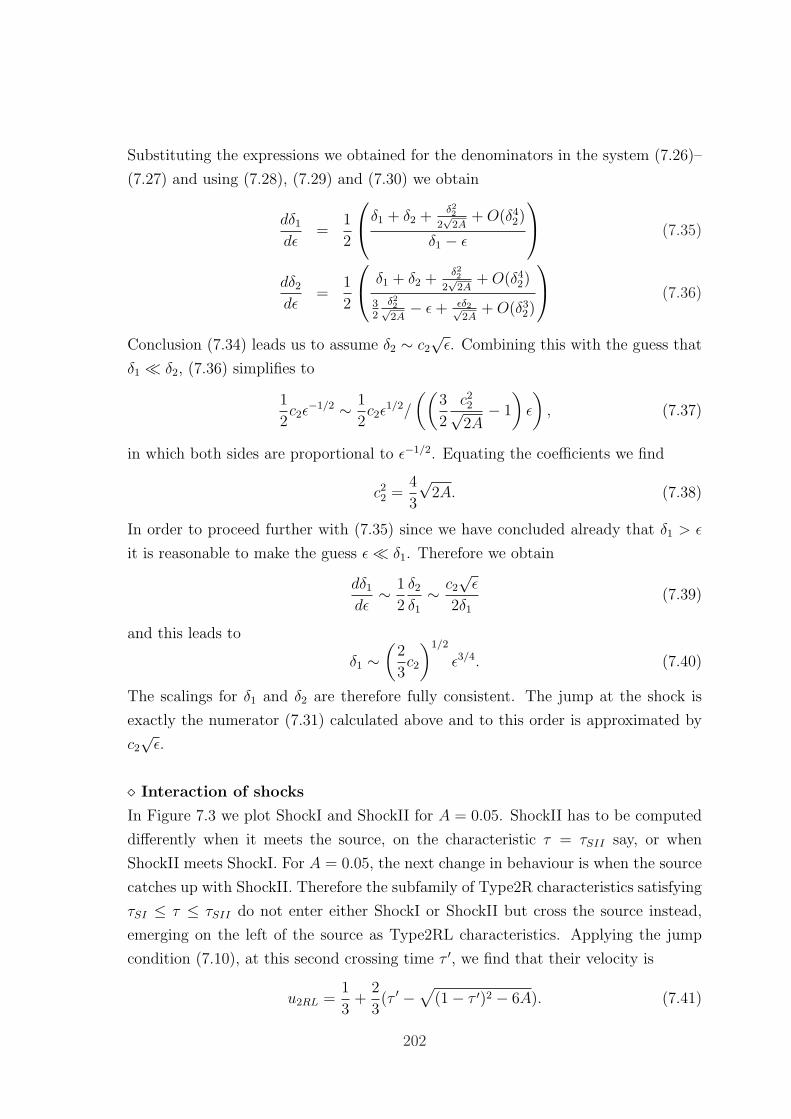
Substituting the expressions we obtained for the denominators in the system (7.26)–
(7.27) and using (7.28), (7.29) and (7.30) we obtain
dδ1dε
=1
2
δ1 + δ2 +
δ222√
2A+O(δ4
2)
δ1 − ε
(7.35)
dδ2dε
=1
2
δ1 + δ2 +
δ222√
2A+O(δ4
2)
32
δ22√2A− ε+ εδ2√
2A+O(δ3
2)
(7.36)
Conclusion (7.34) leads us to assume δ2 ∼ c2√ε. Combining this with the guess that
δ1 ¿ δ2, (7.36) simplifies to
1
2c2ε
−1/2 ∼ 1
2c2ε
1/2/
((3
2
c22√2A
− 1
)ε
), (7.37)
in which both sides are proportional to ε−1/2. Equating the coefficients we find
c22 =4
3
√2A. (7.38)
In order to proceed further with (7.35) since we have concluded already that δ1 > ε
it is reasonable to make the guess ε¿ δ1. Therefore we obtain
dδ1dε
∼ 1
2
δ2δ1∼ c2
√ε
2δ1(7.39)
and this leads to
δ1 ∼(
2
3c2
)1/2
ε3/4. (7.40)
The scalings for δ1 and δ2 are therefore fully consistent. The jump at the shock is
exactly the numerator (7.31) calculated above and to this order is approximated by
c2√ε.
¦ Interaction of shocks
In Figure 7.3 we plot ShockI and ShockII for A = 0.05. ShockII has to be computed
differently when it meets the source, on the characteristic τ = τSII say, or when
ShockII meets ShockI. For A = 0.05, the next change in behaviour is when the source
catches up with ShockII. Therefore the subfamily of Type2R characteristics satisfying
τSI ≤ τ ≤ τSII do not enter either ShockI or ShockII but cross the source instead,
emerging on the left of the source as Type2RL characteristics. Applying the jump
condition (7.10), at this second crossing time τ ′, we find that their velocity is
u2RL =1
3+
2
3(τ ′ −
√(1− τ ′)2 − 6A). (7.41)
202
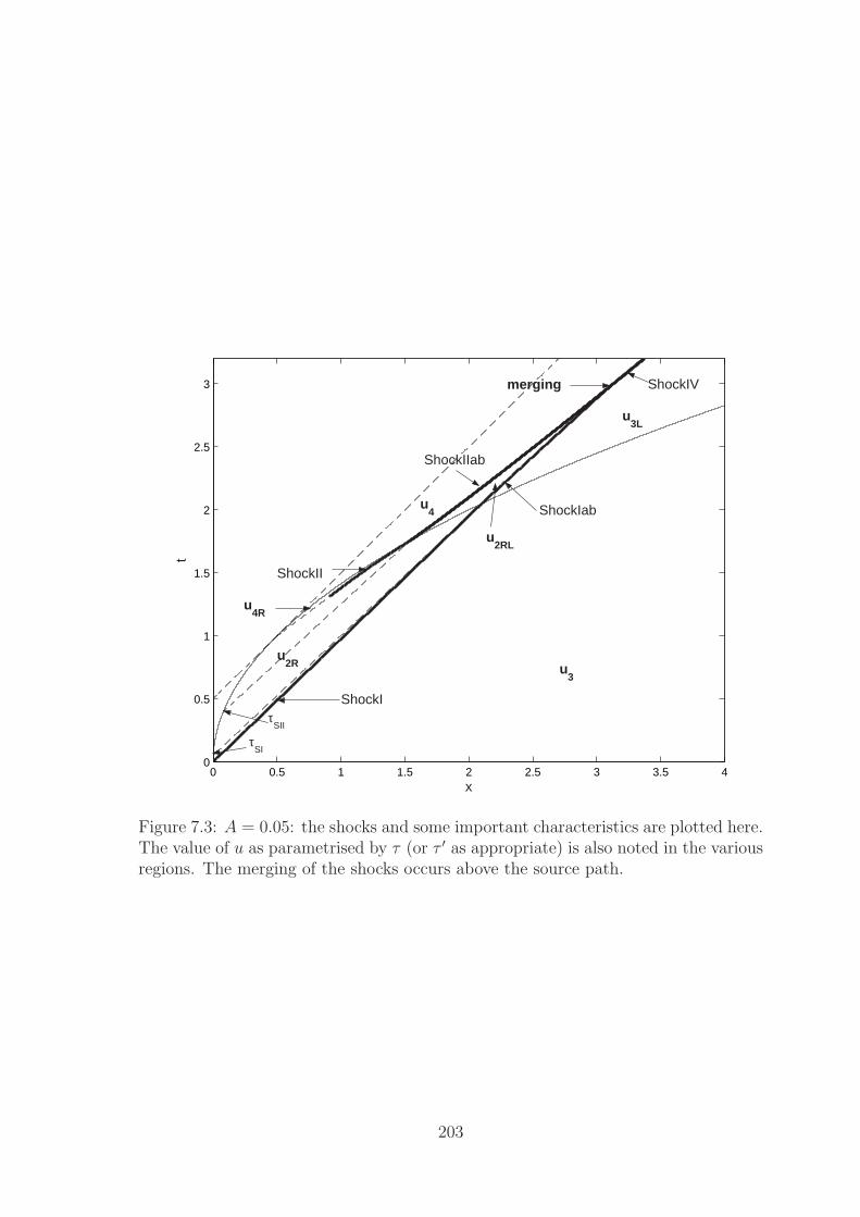
0 0.5 1 1.5 2 2.5 3 3.5 40
0.5
1
1.5
2
2.5
3
x
t
ShockI
ShockII
ShockIab
ShockIVmerging
u3
u3L
u4
ShockIIab
u4R
u2R
u2RL
τSI
τSII
Figure 7.3: A = 0.05: the shocks and some important characteristics are plotted here.The value of u as parametrised by τ (or τ ′ as appropriate) is also noted in the variousregions. The merging of the shocks occurs above the source path.
203
Below we derive the relation (7.41), which is valid for both positive and negative A.
However for A > 0 (7.41) holds only for the restricted range of τ ′ ≥ 1 +√
6A.
From the jump relation (7.17) we have the following relation between u2RL and
u2R
u2RL = τ ′ −√
(τ ′ − u2R)2 − 2A. (7.42)
Since any Type2R characteristic is a chord of the parabola x = t2/2, it satisfies the
relationτ ′2
2=τ 2
2+ u2R(τ)(t− τ) (7.43)
which gives the relation
τ ′ = 2u2R(τ)− τ = τ + 2√
(1− τ)2 − 2A. (7.44)
Inserting (7.44) in (7.42) we obtain
u2RL(τ ′, τ) = 2u2R(τ)− 1 = τ ′ + τ − 1. (7.45)
Therefore to express u2RL in terms of τ ′ only we need to find τ as a function of τ ′ by
solving (7.44) for τ . Rearranging (7.44) we obtain the quadratic
3(1− τ)2 + 2(1− τ ′)(1− τ) + 8A− (τ ′ − 1)2 = 0 (7.46)
which gives
(1− τ) =τ ′ − 1
3± 2
3
√(1− τ ′)2 − 6A (7.47)
and selecting the positive root and inserting in (7.45) we obtain (7.41). The positive
root is selected by checking that when A = 0 (7.47) gives τ ′ = 2− τ as in (7.44).
ShockII will continue above the source; its continuation, called ShockIIab from
now on, will have on the left Type4 characteristics and on the right Type2RL char-
acteristics. The system (7.26)–(7.27) holds again for ShockIIab, but with u1 replaced
by u4 and u2 replaced by u2RL (as indicated in Figure 7.3). Similarly, for the contin-
uation of ShockI above the source, to be called ShockIab, the system (7.26)–(7.27) is
to be solved again, but with u1 replaced by u2RL and u2 replaced by u3L (as indicated
in Figure7.3). ShockIab and ShockIIab are shown in Figure 7.3.
ShockIab and ShockIIab merge at some time tmerge, and the resulting shock, called
ShockIV, has on the left Type4 characteristics and on the right Type3L characteristics,
and obeys again the system (7.26)–(7.27), with u1 replaced by u4 and u2 replaced by
u3L. The merging point and ShockIV are indicated in Figure 7.3. Summarising, we
used the ordinary differential equation (7.21) for determining ShockI and the system
(7.26)–(7.27) for determining ShockII, ShockIIab, ShockIab and ShockIV.
204
When defining the initial conditions for each shock numerically, a careful procedure
similar to that for ShockII was followed for ShockIab and ShockIIab, since (7.26) has
a singularity at the starting point for these. Below we list the initial conditions for
the shocks.
• For ShockIab: τ1 = τ2 = ts = τSI + 2√
(1− τSI)2 + 2A.
• For ShockIIab: τ1 = τ2 = ts = τSII + 2√
(1− τSII)2 + 2A.
Note that τ1 and τ2 and ts stand for different quantities according to the shock we
are considering.
• For ShockIV the initial conditions on τ1 and τ2 are determined by identifying the
τ ′c that parametrises the common Type2RL characteristic entering the merging point
of ShockIab and ShockIIab. Then for this τ ′c we identify the corresponding τ that
parametrises the Type4 characteristic entering the merging point from the left and
this provides the initial condition for τ1 for ShockIV. We also use τ ′c to identify the τ
of the Type3L characteristic entering the merging point from the right, and the latter
value provides the initial condition for τ2 for ShockIV.
As A increases we expect the merging of ShockIab and ShockIIab to occur at
an earlier time. We find numerically that for A ≈ 0.109 the merging happens on
the source path, and for values of A larger than 0.109 the merging occurs below the
source. (Therefore the threshold value A = 0.27551, mentioned earlier, proves to be
irrelevant.)
As an example of this we present the case A = 0.2 in Figure 7.4. The shock formed
when ShockI merges with ShockII, called ShockIII, can now be calculated analytically
using (7.21) since it has on the left Type4R characteristics and on the right Type3
characteristics that have velocity 1. Integrating (7.21) with u = u4R we find
ts(u) =23u3 − u2 + C
(u− 1)2(7.48)
where the constant C is calculated numerically as a function of the merging point.
ShockIV now starts where ShockIII meets the source and (7.26) has a singularity
there. The initial conditions for ShockIV are τ1 = τ2 = tsIII where tsIII is the time of
crossing of ShockIII and the source (and can be determined analytically). In Figure
7.4 we also plot the sonic tangent and the τ = 1 characteristic and label the various
regions of u.
Finally, for values of A ≥ 1/2, Type2R characteristics have all entered ShockI
so ShockII is absent and ShockIII is formed as the continuation of ShockI. ShockIV
starts at the source where ShockIII crosses. We display ShockI, ShockIII and ShockIV
in Figure 7.5.
205
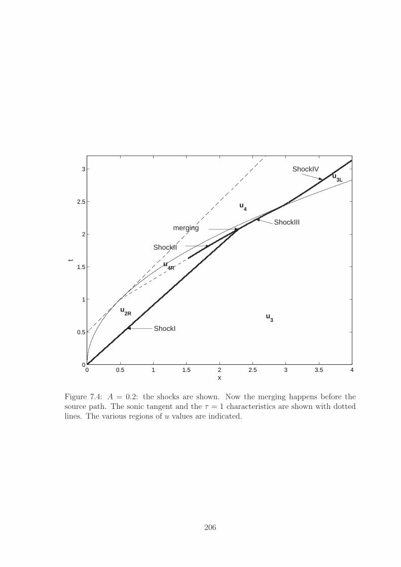
0 0.5 1 1.5 2 2.5 3 3.5 40
0.5
1
1.5
2
2.5
3
ShockI
ShockII
mergingShockIII
u3
u3L
u4
u4R
u2R
x
t
ShockIV
Figure 7.4: A = 0.2: the shocks are shown. Now the merging happens before thesource path. The sonic tangent and the τ = 1 characteristics are shown with dottedlines. The various regions of u values are indicated.
206
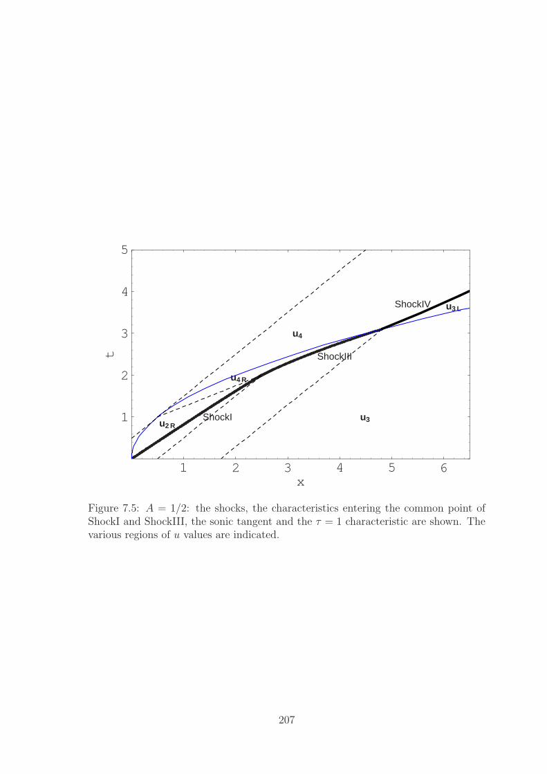
1 2 3 4 5 6x
1
2
3
4
5
t
ShockI
ShockIII
ShockIV
u3
u3 L
u4 R
u4
u2 R
Figure 7.5: A = 1/2: the shocks, the characteristics entering the common point ofShockI and ShockIII, the sonic tangent and the τ = 1 characteristic are shown. Thevarious regions of u values are indicated.
207
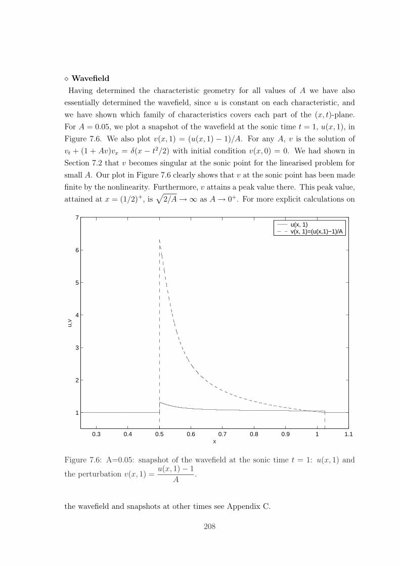
¦ Wavefield
Having determined the characteristic geometry for all values of A we have also
essentially determined the wavefield, since u is constant on each characteristic, and
we have shown which family of characteristics covers each part of the (x, t)-plane.
For A = 0.05, we plot a snapshot of the wavefield at the sonic time t = 1, u(x, 1), in
Figure 7.6. We also plot v(x, 1) = (u(x, 1) − 1)/A. For any A, v is the solution of
vt + (1 + Av)vx = δ(x − t2/2) with initial condition v(x, 0) = 0. We had shown in
Section 7.2 that v becomes singular at the sonic point for the linearised problem for
small A. Our plot in Figure 7.6 clearly shows that v at the sonic point has been made
finite by the nonlinearity. Furthermore, v attains a peak value there. This peak value,
attained at x = (1/2)+, is√
2/A→∞ as A→ 0+. For more explicit calculations on
0.3 0.4 0.5 0.6 0.7 0.8 0.9 1 1.1
1
2
3
4
5
6
7
x
u,v
u(x, 1)v(x, 1)=(u(x,1)−1)/A
Figure 7.6: A=0.05: snapshot of the wavefield at the sonic time t = 1: u(x, 1) and
the perturbation v(x, 1) =u(x, 1)− 1
A.
the wavefield and snapshots at other times see Appendix C.
208
7.3.2 Negative force (A < 0)
¦ Characteristic diagram and the shock
We now consider the A < 0 problem. In this case, we already noted that Type2R
characteristics are slower than Type3 characteristics and therefore an empty region is
formed between them. To resolve this, we introduce the expansion fan characteristics
x = λt, with√
1− 2|A| ≤ λ ≤ 1. We will call the expansion fan characteristics
Type5. Clearly, |A| = 1/2 is a threshold value, and we start with the case |A| < 1/2.
A characteristic in the expansion fan continues up to the source, crosses it at time τ ,
and then deflects with velocity
u5L(τ) = τ −√τ 2
4+ 2|A|. (7.49)
A Type3 characteristic crosses the source once at time τ and slows down afterwards
with velocity u3L = τ−√
(τ − 1)2 + 2|A|. The Type2R characteristics cross the source
again and emerge on the left of the source with a smaller velocity u2RL (as given by
(7.41) with A = −|A|). They therefore cross the Type1 characteristics coming from
the left. Hence, we have to fit a shock on the left of the source. This shock starts
on the source at the time t = 1 −√
2|A| when the leftmost Type2R characteristic
becomes tangent to the source. This corresponds to a Type2RL characteristic with
velocity 1 − 2√
2|A| which crosses a Type1 characteristic at the source. Using this
fact we calculate the initial velocity of the shock there, using the Rankine-Hugoniot
condition,
dx/dt = (1 + (1− 2√
2|A|))/2 = 1−√
2|A|, (7.50)
and we conclude that the shock starts off tangentially to the source. Since the Type1
characteristics have constant velocity equal to 1, this shock can be calculated analyt-
ically, by integrating (7.21). We find
(u2RL(τ ′)− 1)2ts = 427
(√
(τ ′ − 1)2 + 6|A|(1 + 6|A|+ (4− 5τ ′)τ ′) +
τ ′(3 + 36|A|+ τ ′(5τ ′ − 9))) + 427− 8|A|
3. (7.51)
where the constant of integration is determined by imposing the initial condition,
ts = 1−√
2|A| at τ ′ = 1−√
2|A|.The shock moves subsequently into the region of the Type5L characteristics, and
then into the region of the Type3L characteristics, while having always Type1 char-
acteristics on the left. The analytical expression for the shock, corresponding to the
209
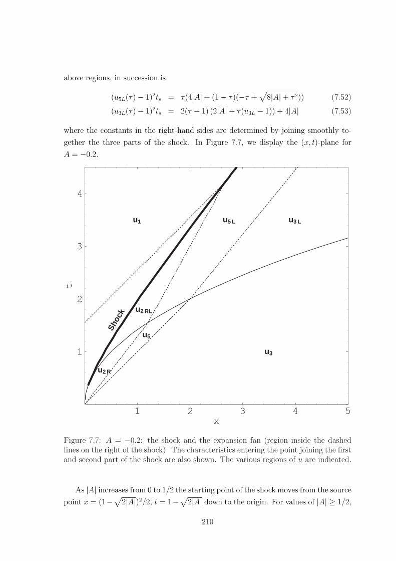
above regions, in succession is
(u5L(τ)− 1)2ts = τ(4|A|+ (1− τ)(−τ +√
8|A|+ τ 2)) (7.52)
(u3L(τ)− 1)2ts = 2(τ − 1) (2|A|+ τ(u3L − 1)) + 4|A| (7.53)
where the constants in the right-hand sides are determined by joining smoothly to-
gether the three parts of the shock. In Figure 7.7, we display the (x, t)-plane for
A = −0.2.
1 2 3 4 5x
1
2
3
4
t
u3
u3 Lu1
u2 R
u2 RL
u5
u5 L
Shoc
k
Figure 7.7: A = −0.2: the shock and the expansion fan (region inside the dashedlines on the right of the shock). The characteristics entering the point joining the firstand second part of the shock are also shown. The various regions of u are indicated.
As |A| increases from 0 to 1/2 the starting point of the shock moves from the source
point x = (1−√
2|A|)2/2, t = 1−√
2|A| down to the origin. For values of |A| ≥ 1/2,
210
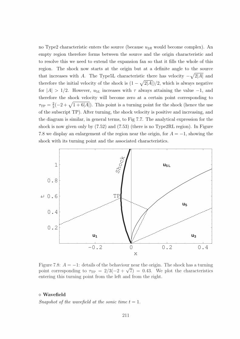
no Type2 characteristic enters the source (because u2R would become complex). An
empty region therefore forms between the source and the origin characteristic and
to resolve this we need to extend the expansion fan so that it fills the whole of this
region. The shock now starts at the origin but at a definite angle to the source
that increases with A. The Type5L characteristic there has velocity −√
2|A| and
therefore the initial velocity of the shock is (1−√
2|A|)/2, which is always negative
for |A| > 1/2. However, u5L increases with τ always attaining the value −1, and
therefore the shock velocity will become zero at a certain point corresponding to
τTP = 23(−2 +
√1 + 6|A|). This point is a turning point for the shock (hence the use
of the subscript TP). After turning, the shock velocity is positive and increasing, and
the diagram is similar, in general terms, to Fig 7.7. The analytical expression for the
shock is now given only by (7.52) and (7.53) (there is no Type2RL region). In Figure
7.8 we display an enlargement of the region near the origin, for A = −1, showing the
shock with its turning point and the associated characteristics.
-0.2 0 0.2 0.4x
0.2
0.4
0.6
0.8
1
t
u3
u3 L
u1
u5
u5 L
Shock
TP
Figure 7.8: A = −1: details of the behaviour near the origin. The shock has a turningpoint corresponding to τTP = 2/3(−2 +
√7) = 0.43. We plot the characteristics
entering this turning point from the left and from the right.
¦ Wavefield
Snapshot of the wavefield at the sonic time t = 1.
211
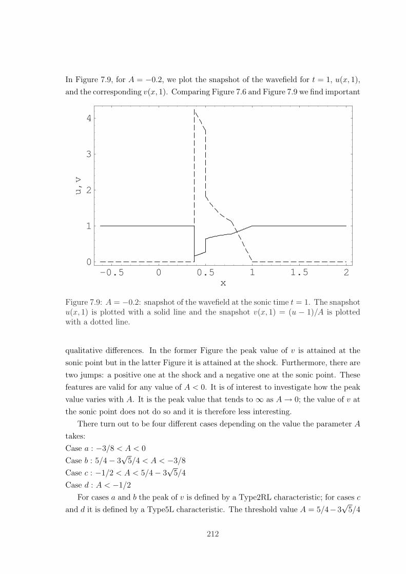
In Figure 7.9, for A = −0.2, we plot the snapshot of the wavefield for t = 1, u(x, 1),
and the corresponding v(x, 1). Comparing Figure 7.6 and Figure 7.9 we find important
-0.5 0 0.5 1 1.5 2x
0
1
2
3
4
u,v
Figure 7.9: A = −0.2: snapshot of the wavefield at the sonic time t = 1. The snapshotu(x, 1) is plotted with a solid line and the snapshot v(x, 1) = (u − 1)/A is plottedwith a dotted line.
qualitative differences. In the former Figure the peak value of v is attained at the
sonic point but in the latter Figure it is attained at the shock. Furthermore, there are
two jumps: a positive one at the shock and a negative one at the sonic point. These
features are valid for any value of A < 0. It is of interest to investigate how the peak
value varies with A. It is the peak value that tends to ∞ as A→ 0; the value of v at
the sonic point does not do so and it is therefore less interesting.
There turn out to be four different cases depending on the value the parameter A
takes:
Case a : −3/8 < A < 0
Case b : 5/4− 3√
5/4 < A < −3/8
Case c : −1/2 < A < 5/4− 3√
5/4
Case d : A < −1/2
For cases a and b the peak of v is defined by a Type2RL characteristic; for cases c
and d it is defined by a Type5L characteristic. The threshold value A = 5/4− 3√
5/4
212
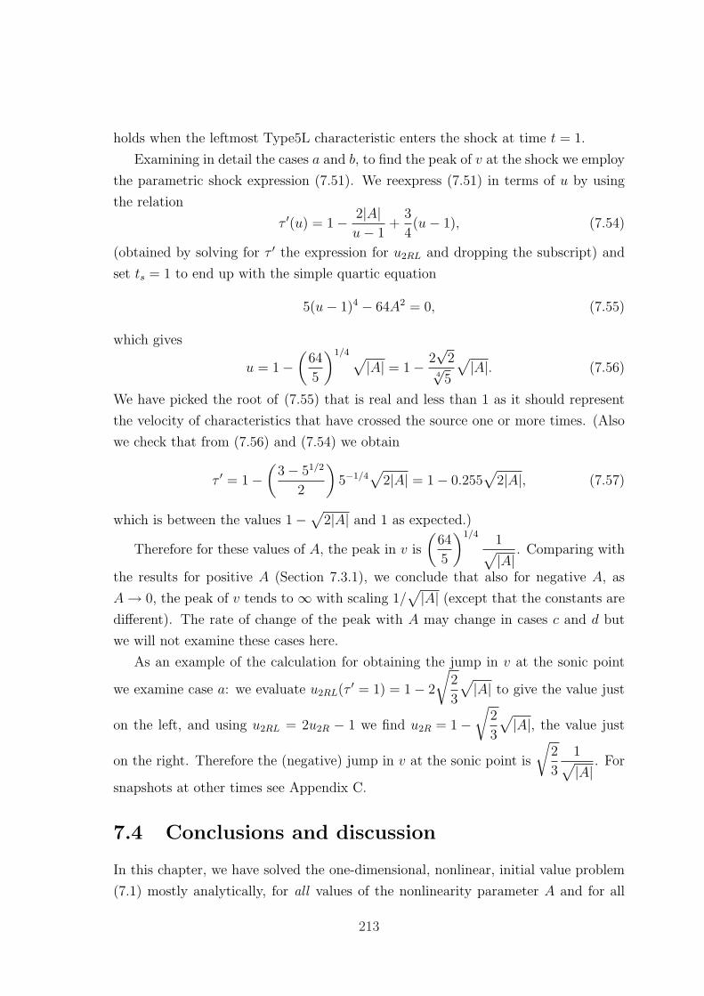
holds when the leftmost Type5L characteristic enters the shock at time t = 1.
Examining in detail the cases a and b, to find the peak of v at the shock we employ
the parametric shock expression (7.51). We reexpress (7.51) in terms of u by using
the relation
τ ′(u) = 1− 2|A|u− 1
+3
4(u− 1), (7.54)
(obtained by solving for τ ′ the expression for u2RL and dropping the subscript) and
set ts = 1 to end up with the simple quartic equation
5(u− 1)4 − 64A2 = 0, (7.55)
which gives
u = 1−(
64
5
)1/4 √|A| = 1− 2
√2
4√
5
√|A|. (7.56)
We have picked the root of (7.55) that is real and less than 1 as it should represent
the velocity of characteristics that have crossed the source one or more times. (Also
we check that from (7.56) and (7.54) we obtain
τ ′ = 1−(
3− 51/2
2
)5−1/4
√2|A| = 1− 0.255
√2|A|, (7.57)
which is between the values 1−√
2|A| and 1 as expected.)
Therefore for these values of A, the peak in v is
(64
5
)1/41√|A| . Comparing with
the results for positive A (Section 7.3.1), we conclude that also for negative A, as
A→ 0, the peak of v tends to ∞ with scaling 1/√|A| (except that the constants are
different). The rate of change of the peak with A may change in cases c and d but
we will not examine these cases here.
As an example of the calculation for obtaining the jump in v at the sonic point
we examine case a: we evaluate u2RL(τ ′ = 1) = 1− 2
√2
3
√|A| to give the value just
on the left, and using u2RL = 2u2R − 1 we find u2R = 1−√
2
3
√|A|, the value just
on the right. Therefore the (negative) jump in v at the sonic point is
√2
3
1√|A| . For
snapshots at other times see Appendix C.
7.4 Conclusions and discussion
In this chapter, we have solved the one-dimensional, nonlinear, initial value problem
(7.1) mostly analytically, for all values of the nonlinearity parameter A and for all
213
points in the (x, t)-plane. This problem constitutes a simple one-dimensional model
for the interaction of nonlinearity with a point force accelerating through the sound
speed. Our solution furnished us with the full details of this interaction. This under-
standing is useful for the various physical problems mentioned in the introduction of
the chapter and which cannot be tackled by analytical means.
In Section 7.2 we have solved the linear approximation of problem (7.1), for small
A in order to show that a singularity is formed at the sonic point x = 1/2, t = 1 which
then propagates along the sonic tangent x = t− 1/2. In Section 7.3.1 we have solved
the full problem (7.1) for all positive A, and in Section 7.3.2 for all negative A. We
obtained the solution by constructing the characteristic diagram in the (x, t)-plane
and resolving multi-valued regions with shocks and empty regions with expansion
fans. For 0 < A < 1/2, there are two shocks which merge later; for A ≥ 1/2 and
all negative A only one shock forms. The solution is entirely analytical for negative
A. For positive A the solution is also analytical, except for some shocks that are
calculated numerically by solving the second-order o.d.e. system (7.26)–(7.27).
Overall, the results are very different qualitatively for the different signs of A,
reflecting the expected physical differences that would come about in the wavefield
when a point force changes direction. However for any non-zero A our solution dis-
plays how the introduction of nonlinearity makes the sonic singularity finite. In order
to show this clearly, for selected positive and negative A, we plotted snapshots of v
at the sonic time t = 1. Furthermore, we found that the peak value of v tends to ∞as A→ 0 with scaling 1/
√|A|.
We assumed uniform acceleration and were thus able to calculate most of the
solution analytically. However, we expect this to be a very useful guide to any scenario
where the source has a monotonically increasing velocity.
214
Chapter 8
Conclusions
We began the thesis with a brief history of sonic boom research and its current
importance for a new SST. We subsequently gave a brief exposition of the established
theory and the major open questions.
In Chapter 2 we presented the equations of gas dynamics, and explained when
these equations simplify into the Euler equations, coupled with the appropriate
Rankine-Hugoniot conditions for fitting shocks into the flow pattern. In this connec-
tion we also proved a new circulation theorem, closely related to Kelvin’s circulation
theorem, Bjerknes’ theorem and Crocco’s theorem, but one that is valid in the pres-
ence of shocks. We showed that the circulation Γ around a closed material curve in an
inviscid gas flow evolves according to an equation that involves the entropy changes
around this curve, excluding the entropy jumps at the shock. We thus proved, in a
rigorous way, that if a uniform transonic or supersonic flow is incident on a thin wing
or a slender rigid body, and the resulting flow contains only weak shocks with strength
of order ε, then the vorticity produced after the shocks is of order ε3. This result was
subsequently needed in Chapter 4 for rigorously justifying the use of potential flow
after a shock is crossed.
In Chapter 3 we started by laying out the basic definitions governing sonic boom
geometry. The notions of a characteristic surface, wavefront, bicharacteristic, ray,
boomray, Mach envelope, and the carpet were defined. Three ways to construct the
Mach envelope were then presented and the relationships between them elucidated.
We also outlined carefully the connection between the theory of characteristics and
geometrical acoustics and showed that the equation for the characteristic surfaces of
the wave equation is precisely the eikonal equation arising at the leading order in the
geometrical acoustics framework. This is often not clear in the sonic boom literature.
We then applied the theoretical results to particular examples and illustrated them
carefully in order to elucidate aspects of the long-range propagation of sound, and in
215
particular of sonic boom in stationary media. (The theory of Geometrical Acoustics
in moving media was briefly presented in Section 3.10 and was used to explain how
stratospheric SSBs may arise.)
We first studied the geometry of the ray surface in the model stratified atmosphere
c = 1/√
1− z. We found that the rays from a stationary source form a fold caustic.
We subsequently calculated the amplitude due to a stationary, sinusoidal source in
this atmosphere. Due to the nature of this particular sound speed profile we were
able to use the full linear wave theory. We showed that inside the caustic there is an
order 1 wavefield which is amplified on the caustic and decays exponentially outside.
These results agreed nicely with the Geometrical Theory of Diffraction.
We then considered a source moving at constant supersonic speed in the same
stratified medium. The governing linear PDE was of mixed type: in the vertical plane
of motion, it was hyperbolic below the sonic height, parabolic at the sonic height, and
elliptic above this height, and could be recast into the Tricomi equation. The boom
reflects from the sonic line, the Mach envelope having the local shape of a Tricomi
cusp there (as illustrated, for example, in Figure 3.27). This Tricomi cusp joins two
qualitatively different parts of the Mach envelope, which we called respectively the
incident part and the reflected part. It is a key fact that the presence of a Tricomi
cusp on the Mach envelope is directly associated with the formation of a fold caustic
of boomrays, and corresponds to focusing of the sonic boom. The fold caustic is
precisely the sonic line (see Figure 3.27); the Tricomi cusp moves on the sonic line at
the local sound speed. In Chapter 6, in a constant-acceleration motion through the
sound speed in a uniform medium, we also saw a qualitatively similar behaviour (see
Figure 6.5): boomrays again formed fold caustics1, and this corresponded to Tricomi
cusps that again moved at the sound speed on the “cusp-locus” curve (6.47).
The geometry of a fold caustic of ordinary rays and that of a fold caustic of
boomrays is similar, and in terms of catastrophe theory they are essentially the same.
This is generally the viewpoint found in the sonic boom literature. However, we
emphasise two important differences:
• Boomrays are curves in (x, t)-space emanating from the source, but for a sta-
tionary harmonic source one generally thinks of rays simply as curves in x-space.
• Rays are emitted by a source in all directions, but boomrays are only emitted
when the source is supersonic, and only at a certain angle to the direction of
motion.
1Two caustics were formed which were symmetric with respect to the direction of motion.
216
Next, through a simple coordinate transformation we used the stationary source
example c = 1/√
1− z to determine the Mach surface for steady motion in three
dimensions in the medium with Prandtl-Glauert parameter B2 = 1− z. In this case
the Tricomi cusp generalised to a focusing curve. The carpet was also determined
analytically and possessed cusps, indicating the location of focusing regions on the
ground.
We then extended the latter example to B2 = 1−|z|, where the sound speed profile
has a minimum, as in a typical (windless) atmosphere. We found that we could still
treat this analytically. Some of the bicharacteristics launched downwards formed a
primary boom carpet, some of those launched upwards formed a secondary carpet,
whereas a third set of bicharacteristics was trapped in the atmosphere and never
reached the ground, resulting in disjoint primary and secondary carpets. Again cusps
were observed at the carpets corresponding to regions of focusing. This behaviour
agreed qualitatively with the behaviour of bicharacteristics in a typical atmosphere,
which was investigated numerically.
We discussed focusing of linear sound waves and weak shock waves at the end
of the chapter in general and also in connection with specific examples. In Chapter
4 we mainly dealt with amplitude questions. We investigated the wavefield around
thin aerofoils or slender axisymmetric bodies moving at constant supersonic speed in
a uniform medium. The starting point was the nonlinear potential equation, derived
exactly from the Euler equations under the assumption of potential flow (as justified
by our results in Chapter 2). We used Matched Asymptotic Expansions (MAE) to
derive consistent approximations of this potential equation in appropriately defined
regions: in the inner region of the MAE (the near-field) we found that the pressure
is governed by a linear wave equation at leading order. However, we showed that
the linear approximation breaks down at a certain distance from the body, due to
small nonlinearities that cumulatively become important. Thus a second region was
introduced, the outer region (or the far-field). In this outer region, the consistent
approximation of the potential equation at leading order is the nonlinear Kinematic
Wave Equation (KWE). An N -wave signature was derived as a solution of this KWE,
exactly for an aerofoil with parabolic shape in two dimensions, and asymptotically
for any thin or slender shape in two or three dimensions. The work in this chapter
formalises Whitham’s rule [124, 125], and the work of Hayes in [51]. The latter
studies accounted only for first-order corrections but our MAE framework allows for
the calculation of the higher orders.
217
In Chapter 5 we extended the work of Chapter 4 in order to incorporate non-
linearities in a consistent way for the long-range propagation of weak shocks in a
stratified atmosphere with wind. This work is new and can be thought of as the
extension of the primary boom results in Chapter 4 (and other literature) to the case
of secondary boom. We sought the wavefield due to a thin, two-dimensional aerofoil
moving supersonically in a general weakly stratified medium with a horizontal wind,
which itself was also weakly stratified. Two small nondimensional parameters were
defined, namely the thickness ratio ε (as in Chapter 4), and the ratio of the aerofoil
length to the scale height of the atmosphere, δ (as in Chapter 3). We have assumed
that δ is much smaller than ε2, an assumption which is reasonable for a typical atmo-
sphere. We also abandoned the assumption of potential flow, since there is already
vorticity in the incident stratified flow, so we worked with the full Euler equations.
We again applied MAE to derive consistent approximations for these equations in
three regions of interest:
• Near the aerofoil the wavefield was determined by linearised wave theory at
leading order. This was the inner region of the MAE method.
• At distances of order L/ε nonlinear effects were important (but not stratification
effects) and we found that the governing PDE at leading order was a KWE. This
was the middle region of the MAE method.
• At distances of order L/δ stratification and nonlinear effects were both of order
1. This was the outer region of the MAE method. We found that the governing
equation at leading order was an inhomogeneous KWE with non-constant co-
efficients. The derived KWE led to a very simple expression for the amplitude
variation along the characteristics.
We noted that the approximations of the Euler equations in the inner region and the
middle region turned out to be the same as those in Chapter 4, in the near-field and
far-field respectively.
Our MAE method blows up near the sonic line where B is small. A fourth re-
gion needs to be introduced with B taken as a third small parameter. Pechuzal
and Kevorkian [91] have undertaken this for the simpler scenario of a homogeneous
medium that has a horizontal linearly stratified wind. They deduced that the consis-
tent approximation of the Euler equations in this sonic region is a nonlinear Tricomi
equation. It remains an open question as to what the analogous equation is for our
scenario.
218
Another point we would like to stress here is that we retained the gravity term
in the Euler momentum equation throughout Chapter 5, in contrast with Chapter 3
where it was neglected by arguing that acoustic and gravity waves were decoupled.
We found that at the order we worked to there was no direct excitation of gravity
waves, even though the motion took place in a gravitationally stratified atmosphere.
This mathematically confirmed our approach in Chapter 3.
Finally, for this chapter it would be interesting to extend the work for studying a
slender body in the same general ambient conditions.
In Chapter 6 we employed linear wave theory to determine the wavefield due
to a point source in various unsteady motions, in two and three dimensions, in the
time domain. In two dimensions we first considered uniform acceleration through the
sound speed, in a uniform medium. We calculated analytically the Mach envelope; it
has Tricomi cusps, qualitatively the same as those on the Mach envelopes for steady
motions in the stratified atmospheres, as seen in Chapter 3. These cusps join two
qualitatively different parts of the envelope. The so-called front, or incident, envelope
is formed in a similar way to the usual Mach wedge of steady supersonic motion, with
the wavefronts touching their envelope from inside. The so-called back or reflected
envelope (also referred to as the acceleration caustic) is formed by wavefronts touching
it from outside. This Tricomi cusp corresponded again to the formation of a fold
caustic of boomrays and again the front envelope was formed by boomrays that have
not touched this fold caustic and the back envelope by boomrays that have touched
the caustic. This is a generic behaviour of all fold caustics and their associated Mach
envelopes, and was illustrated in detail in all the scenarios we examined in this thesis,
namely steady motion in a stratified medium (in Chapter 3), acceleration through
the sound speed in a uniform medium (in Chapter 6) and manoeuvring in a uniform
medium (in Chapter 6).
In order to determine the wavefield near the Mach envelope for the accelerating
motion in two dimensions we devised a simple approximation method in the time
domain: we found a finite jump at the front envelope and logarithmic singularities
at the back envelope. The appearance of these singularities violates the assumption
of small disturbances underlying the linear theory. This suggests that nonlinearity or
damping have to be re-introduced into the equations. Experiments by Sturtevant and
Kulkany have shown that in some circumstances, nonlinearity is the limiting factor.
The link of our work with the existing literature is that the logarithmic singularities
we identified correspond exactly to the infinite peaks of the U -wave formed when
the N -wave reflects from the fold caustics. Our method was based on the fact that
219
for a uniform medium we can work with the wavefield integral rather than the wave
equation itself, treating the time t as a parameter. This spared us the need to look
for local approximations of the wave equation near the focusing regions, which is the
current method in the literature.
We also considered a source that decelerates uniformly after initially travelling
at a constant supersonic speed. We found that the geometry of the Mach envelope
is very different from that of the accelerating motion. The Mach envelope does not
have a Tricomi cusp (or equivalently no fold caustic is formed) and although focusing
occurs when the source goes subsonic, it is restricted to a single point. We calculated
the wavefield near the Mach envelope, using a similar simple approximation method
as for the acceleration problem: we found that the wavefield is finite for all times
except at the focusing point. This indicates that nonlinearity is likely to be far less
crucial in the prediction of amplitudes in decelerating motion than in accelerating
motion.
We then considered a point source accelerating uniformly through the sound speed,
in three dimensions. The Mach envelope is just a conical generalisation of the Mach
envelope in two dimensions but the wavefield exhibits a very different behaviour due to
the difference between the two-dimensional and three-dimensional Riemann function.
The wavefield tends to infinity on one side of the envelope and is finite on the other
side. It would be interesting to investigate what these singularities become in the
case of an extended source.
Moreover, at the end of Chapter 6 we looked at a uniformly accelerating motion
through the sound speed in the stratified medium c = 1/√
1− z: in Figure 6.25 we
observed that the reflected envelope itself developed cusps which corresponded to a
cusp caustic of boomrays.
The results of Chapter 6 for accelerating motion through the sound speed in
two and three dimensions motivated us to investigate the effect of nonlinearity on
singularities arising when a source goes through the sound speed. However, it is a
formidable task to solve the nonlinear problem in two or three dimensions. What we
have been able to achieve instead in Chapter 7 is to solve a related one-dimensional
nonlinear problem. We considered ut+uux = Aδ(x− t2/2), with the initial condition
u = 1 at t = 0. This is a model for a locally forced kinematic wave in which the
force accelerates through the sound speed at the sonic time t = 1. In the linear
approximation, when the nonlinearity parameter A is small, there is a singularity
at the sonic point, which propagates along the characteristic from that point. (The
propagation of this sonic singularity is also a feature of higher-dimensional problems.)
220
However in such sonic singularities the amplitude may be limited by nonlinearity
or damping. We thus produced a global solution of this PDE, valid for arbitrary
A and which is in most regions analytical. As A varies, the qualitative features
of the characteristic diagram change, but for all A we found that the introduction
of nonlinearity leads to a finite amplitude at the sonic point. It still remains an
interesting open question as to whether the introduction of nonlinearity regularises
the singularities in two or three dimensions. It would also be interesting to pinpoint
whether our one-dimensional problem could arise as a consistent approximation of
the Euler equations. A possible scenario would be the forced acceleration of a body
along a tube of gas, so that the drag would effectively exert a point force on the gas.
221
Appendix A
Transport Theorem for an opencurve
A Transport Theorem for open curves with time-varying endpoints, was used in the
derivation of the Circulation Theorem for a compressible flow that takes shocks into
account, in Chapter 2. We called this theorem KCTS, where the S in the end is to
signify that is valid in the presence of shocks.
The derivation was based in breaking up the closed curve (or circuit) of fluid
elements C into open subcurves separated by shock fronts.
We consider one such subcurve and we parametrise it with s and t, where each
s corresponds to a given fluid element in the gas and t is time. Such a parametric
method is standard in the derivation of Kelvin’s circulation theorem. With this
parametrisation we have∂x
∂t(s, t) = u(x(s, t), t). (A.1)
Let the endpoints of C be labelled by P and Q. They correspond respectively to
parameter values sP and sQ such that
P(t) = x(sP (t), t), Q(t) = x(sQ(t), t). (A.2)
For circulation theorems we are particularly interested in the rate of change of the
circulation
Γ =
∫
Cu.dx, (A.3)
but here we will show a general result that is valid for any vector field, say a(x, t).
We let
I =
∫ Q
P
a(x, t).dx, (A.4)
222
and with the parametrisation introduced above, (A.4) becomes
I =
∫ sQ
sP
a(x(s, t), t).∂x
∂sds. (A.5)
Therefore the total derivative of I
dI
dt=
d
dt
∫ sQ
sP
a(x(s, t), t).∂x
∂sds; (A.6)
applying the Fundamental Theorem of Calculus we have
dI
dt= a(Q).
∂x
∂s|sQsQ − a(P).
∂x
∂s|sPsP +
∫ sQ
sP
∂
∂t
(a(x(s, t), t).
∂x
∂s
)ds. (A.7)
We let the third term in (A.7) be
J =
∫ sQ
sP
∂
∂t
(a(x(s, t), t).
∂x
∂s
)ds. (A.8)
and this, using ui =∂xi∂t
, is written in component form as
J =
∫ sQ
sP
(∂ai∂t
+ uj∂ai∂xj
)∂xi∂s
ds+
∫ sQ
sP
aj∂uj∂s
ds. (A.9)
Integrating by parts the second integral in (A.9) we get∫ sQ
sP
aj∂uj∂s
ds = [ajuj]sQsP−
∫ sQ
sP
uj∂aj∂s
ds
= a(Q).u(Q)− a(P).u(P)−∫ Q
P
uj∂aj∂xi
dxi. (A.10)
Substituting (A.10) into (A.9) and returning to (A.7) we have
dI
dt= a(Q).
(u(Q) +
∂x
∂ssQ
)− a(P).
(u(P) +
∂x
∂ssP
)
+
∫ Q
P
(∂ai∂t
+ uj∂ai∂xj
− uj∂aj∂xi
)dxi. (A.11)
Rewriting the first two terms using (A.2) and using
uj
(∂ai∂xj
− ∂aj∂xi
)= ((∇×a)× u)i, (A.12)
we finally have that the total derivative of the line integral I, for any vector field a is
dI
dt= a(Q).Q− a(P).P +
∫ Q
P
(∂a
∂t+ (∇×a)× u
).dx. (A.13)
Note that another, more geometrical, way to derive the above Transport Theorem
exists (see [8]) but we are not going to give it here.
223
Appendix B
Stationary-phase method for sonicboom problems
In this appendix we will present an alternative way for deriving the Mach envelope,
in two dimensions for any unsteady supersonic motion in a straight line. The method
also provides a classification of the Mach envelope points, according to the sign of
the eigenvalues of an appropriately defined matrix and thus gives a clear link of the
frequency domain to the time domain.
We consider a point source moving horizontally on the trajectory (x0(t), 0). A
small disturbance due to this point source is governed by the linear wave equation
and initial conditions
utt −∇2 u = δ(x− x0(t))δ(z), (B.1)
u = ut = 0 at t = 0. (B.2)
(We have taken c0 = 1.) Taking the Fourier Transform of (B.1)–(B.2) with respect
to x and z we have
utt + k2u = exp(ik1x0(t)), (B.3)
u = ut = 0 at t = 0., (B.4)
where k =√k2
1 + k22. Solving the ODE problem (B.3)–(B.4) we have
u(k1, k2, t) =
∫ t
0
eik1x0(τ) sin k(t− τ)
kdτ. (B.5)
Taking the inverse Fourier transform of (B.5) we obtain
u(x1, z, t) =1
4π2
∫ ∞
−∞
∫ ∞
−∞
∫ t
0
eik1(x0(τ)−x)e−ik2zsin k(t− τ)
kdτdk1dk2, (B.6)
224
which can also be written as
u(x1, z, t) = − i
8π2
∫ ∞
−∞
∫ ∞
−∞
∫ t
0
eik1(x0(τ)−x1)e−ik2z(eik(t−τ) − e−ik(t−τ))k
dτdk1dk2.
(B.7)
From now on we will let
JA =
∫∫∫eitφ
kdτdk1dk2, JB =
∫∫∫eitψ
kdτdk1dk2, (B.8)
where the phase functions for JA and JB are respectively
φ =k1(x0(τ)− x1)− k2z + k(t− τ)
t, ψ =
k1(x0(τ)− x1)− k2z − k(t− τ)
t. (B.9)
Therefore we have
8π2u = −i(JA − JB). (B.10)
Below we determine the stationary points of φ and ψ as a first step towards developing
stationary-phase approximations to the integrals JA and JB (with t considered to be
a large parameter) and show that the classical stationary-phase method cannot be
used to calculate wavefields. However, the method is still very useful because even
though it eventually breaks down, it provides the geometry of the Mach envelope.
Since ψ(−k) = −φ(k) there is a 1-1 correspondence between the stationary points
of φ and ψ, and it is sufficient to calculate only the quantities associated with the phase
φ. In order to determine the stationary point(s) of JA, sA say, we set respectively
∇φ|sA= 0. (B.11)
We will make a convenient change of notation from (k1, k2, τ) to s = (s1, s2, s3) so
that the stationary points are denoted by sA = (sA1, sA2, sA3). Writing (B.11) as a
system of three equations in the three unknowns sA1, sA2, sA3 we have
∂φ
ds1
= 0 ⇒ x0(sA3)− x
t+sA1
kA
(1− sA3
t
)= 0, (B.12)
∂φ
ds2
= 0 ⇒ −zt
+sA2
kA
(1− sA3
t
)= 0, (B.13)
∂φ
ds3
= 0 ⇒ sA1x′0(sA3)− kA
t= 0, (B.14)
where kA =√s2A1 + s2
A2. From (B.14) we have
x′0(sA3) =kAsA1
. (B.15)
225
Reverting to the original notation (B.15) gives
x′0(τ0) =k0
k10
. (B.16)
Letting k10 = k0 cos θ, k20 = k0 sin θ in (B.16) we recover the boomray condition
cos θ =1
x′0(τ0), (B.17)
which has been discussed in detail in Chapter 3, p. 37. The boomray condition
cannot hold if |x′0(τ0)| < 1, which simply means that when the source motion is
subsonic there are no boomrays. Also combining (B.12) and (B.13) we obtain
(x0(τ0)− x)2 + z2 = (t− τ0)2, (B.18)
the circular wavefronts evaluated at the stationary point. The points defined by the
relations (B.17) and (B.18) are precisely the Mach envelope points. Therefore the
current method leads to expressions equivalent to the Mach envelope equations for
any general motion on the horizontal line (see expressions (6.22) and (6.23)). For any
τ such that the boomray passes through (x, z) at t, there is a corresponding half-line
of (k10, k20) vectors. The stationary points are therefore not isolated and we now
investigate this degeneracy.
B.1 Classification of the Mach envelope points
We proceed to determine the Hessian matrix of φ, which we will call A:
Ajk =∂2φ
dsjdsk|sA, . (B.19)
A is a symmetric matrix and thus only six entries need to be calculated:
A11 =k2
20
k30
(1− τ0
t
), A12 = −k10k20
k30
(1− τ0
t
), A13 =
x′0(τ0)t
− k10
k0t
A22 =k2
10
k30
(1− τ0
t
), A23 = −k20
k0t, A33 =
k10
tx′′0(τ0).
The determinant is
detA = −(t− τ0)(−x′0(τ0)k10 + k0)2
k30t
3= 0, (B.20)
226
having used the boomray condition (B.16). Therefore A is singular, and one of its
three eigenvalues is zero, for any two-dimensional supersonic motion. The eigenvalues
are
λ1 = 0, λ2,3 =C2
2± 1
2
√C2
2 + 4C1, (B.21)
where C1 = −λ2λ3 =x′0(τ0)
2 − 1
t2− x′′0(τ0)x′0(τ0)
t− τ0t2
, (B.22)
and C2 = λ2 + λ3 =x′′0(τ0)x′0(τ0)
k0
t+t− τ0k0t
. (B.23)
The subscripts “2” and “3” refer respectively to the positive and negative signs in
front of the square root in (B.21). We expect a qualitative change in a Mach envelope
point when an eigenvalue changes sign. We recall that the Mach envelope equations
are determined by Q = 0,∂Q
∂τ= 0 where
Q = (t− τ)2 − (x− x0(τ))2 − z2 = 0. (B.24)
Taking the second derivative of Q with respect to τ we have
∂2Q
∂τ 2= −2(x′0
2 − 1) + 2(x− x0(τ))x′′0. (B.25)
Using the first envelope equation (6.22) we have
∂2Q
∂τ 2= −2(x′0
2 − 1)− 2(t− τ)x′′0x′0, (B.26)
and from (B.26) and (B.22) we conclude that
∂2Q
∂τ 2= 2t2λ2λ3. (B.27)
Relation (B.27) gives a very useful classification of the Mach envelope points. Before
stating this classification criterion for the general case of a source moving with arbi-
trary velocity on a straight line, we will present the paradigm problem of a constant-
acceleration motion through the sound speed. In this case
∂2Q
∂τ 2= 2t2λ2λ3 = −2
τ 3 − t
τ. (B.28)
We have already studied and plotted the Mach envelope for this in Chapter 6. There
we found that it consists of a front envelope which the wavefronts envelope from
inside, and a back envelope which the wavefronts envelope from outside. For the
227
back envelope we had identified that∂2Q
∂τ 2> 0 and therefore 1 < τ < t1/3, and for
the front envelope we had identified that∂2Q
∂τ 2< 0 and therefore t1/3 < τ < t. This
consistuted the algebraic criterion of p. 156. Now this criterion can be reinterpreted
more lucidly in terms of the product of the eigenvalues of the Hessian matrix A: since
λ2λ3 = −τ3 − t
τt2we conclude that on the
• front envelope: t1/3 < τ < t⇔ λ2λ3 < 0 ⇔ ∂2Q
∂τ 2< 0,
• back envelope: 1 < τ < t1/3 ⇔ λ2λ3 > 0 ⇔ ∂2Q
∂τ 2> 0.
The front and back envelope join when λ2λ3 = 0,∂2Q
∂τ 2= 0, and Q has a point
of inflexion there. We already know that this common point is a cusp. Having
established these resuts we can proceed to state the following general assertion “For
a general two-dimensional supersonic motion of a point source in a straight line (and
with a uniform ambient medium) a Mach envelope point can only be one of the
following three types:
Type a.∂2Q
∂τ 2< 0 ⇔ λ2λ3 < 0: the envelope point belongs to an envelope part that
is formed by wavefronts enveloping it from inside (such as the Mach wedge in
steady motion and the front envelope of the constant-acceleration motion).
Type b.∂2Q
∂τ 2= 0 ⇔ λ2λ3 = 0: cusp
Type c.∂2Q
∂τ 2> 0 ⇔ λ2λ3 > 0: the envelope point belongs to an envelope part which
wavefronts envelope from outside (such as the back envelope of the constant-
acceleration motion).”
Note that it is λ3 that changes sign when going from the front to the back envelope.
This assertion gives consisely the relation of the frequency domain to the time
domain in sonic boom problems.
B.2 Wavefield
We have established above a general method to classify the Mach envelope points.
This method was set up as a stationary-phase method and the next question, af-
ter determining the stationary points, is whether it can be employed to determine
228
amplitudes, for two-dimensional sonic boom problems. Note that we have already
calculated such amplitudes for steady flight, a uniformly accelerating flight, and a
uniformly decelerating flight through a time-domain method in Chapter 6.
The task is to determine a consistent approximation of the integral (B.6). Letting
(k1, k2) = (k cos θ, k sin θ), (B.29)
we have from (B.6) that
u(x, z, t) =1
4π2
∫ ∞
k=0
∫ θ=2π
θ=0
∫ t
0
eik((x0(τ)−x) cos θ−z sin θ) sin k(t− τ)dτdθdk. (B.30)
The k integral is not (classically or Lebesgue) convergent so it can only be inter-
preted in terms of distribution theory. The classical stationary-phase approximation
breaks down because the contributions from all wavenumbers are important (instead
of a certain interval of k dominating the integral). This arises because sound is not
dispersive (in this approximation). Note that if we evaluate the integral over k as a
distribution by
∫ ∞
0
eikpdk = πδ(p) +i
p, (B.31)
then we recover exactly the usual integral representation of u, as cited on p. 143.
(Noting that u here is the pressure p in the notation of Chapter 6).
229
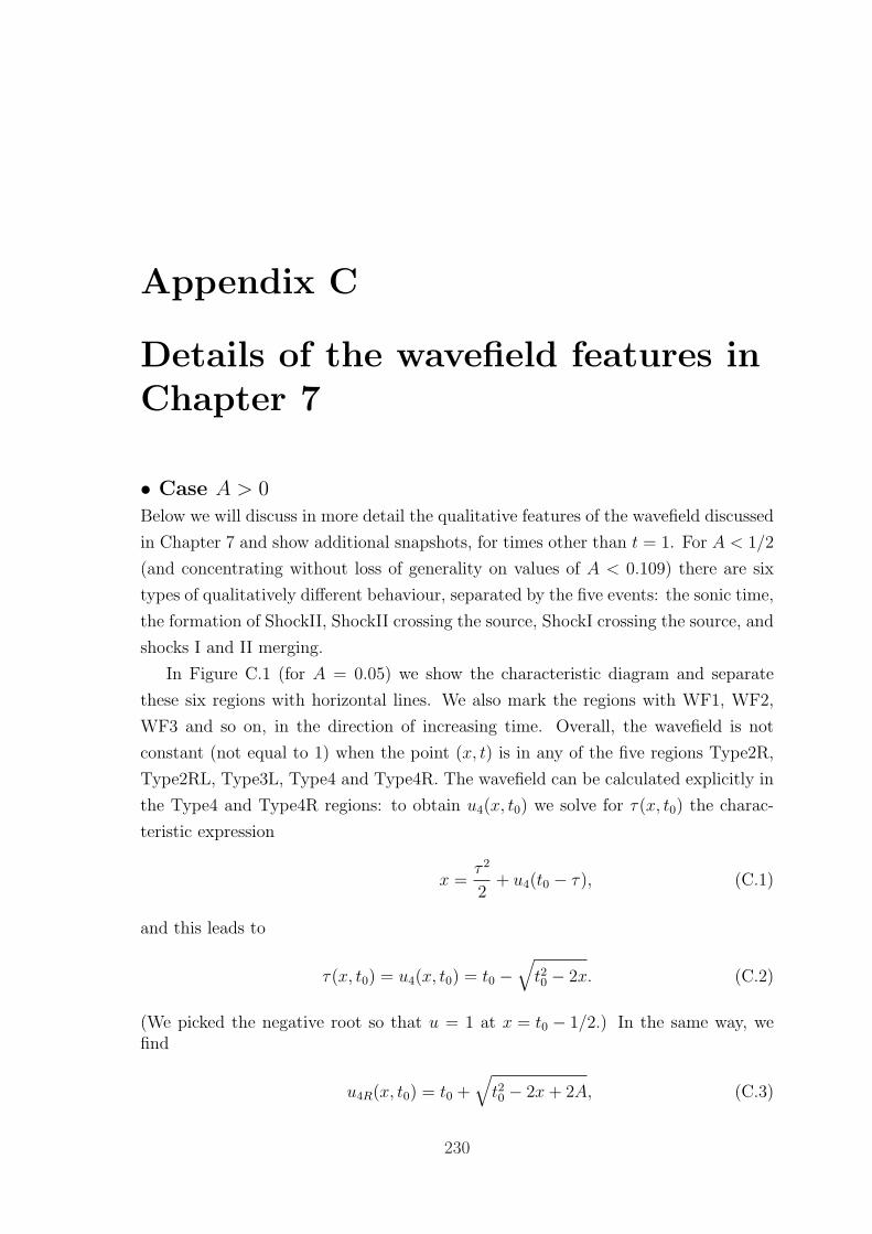
Appendix C
Details of the wavefield features inChapter 7
• Case A > 0Below we will discuss in more detail the qualitative features of the wavefield discussed
in Chapter 7 and show additional snapshots, for times other than t = 1. For A < 1/2
(and concentrating without loss of generality on values of A < 0.109) there are six
types of qualitatively different behaviour, separated by the five events: the sonic time,
the formation of ShockII, ShockII crossing the source, ShockI crossing the source, and
shocks I and II merging.
In Figure C.1 (for A = 0.05) we show the characteristic diagram and separate
these six regions with horizontal lines. We also mark the regions with WF1, WF2,
WF3 and so on, in the direction of increasing time. Overall, the wavefield is not
constant (not equal to 1) when the point (x, t) is in any of the five regions Type2R,
Type2RL, Type3L, Type4 and Type4R. The wavefield can be calculated explicitly in
the Type4 and Type4R regions: to obtain u4(x, t0) we solve for τ(x, t0) the charac-
teristic expression
x =τ 2
2+ u4(t0 − τ), (C.1)
and this leads to
τ(x, t0) = u4(x, t0) = t0 −√t20 − 2x. (C.2)
(We picked the negative root so that u = 1 at x = t0 − 1/2.) In the same way, wefind
u4R(x, t0) = t0 +√t20 − 2x+ 2A, (C.3)
230
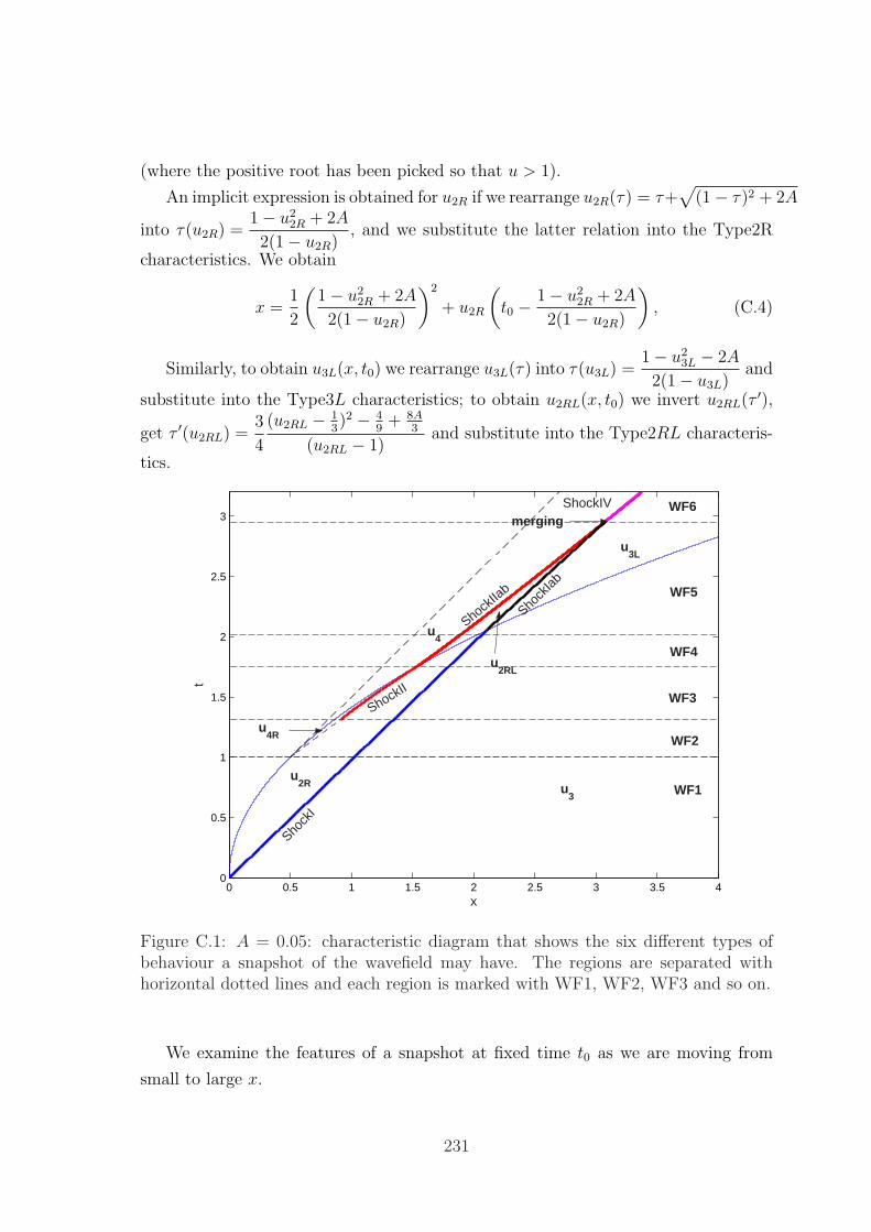
(where the positive root has been picked so that u > 1).
An implicit expression is obtained for u2R if we rearrange u2R(τ) = τ+√
(1− τ)2 + 2A
into τ(u2R) =1− u2
2R + 2A
2(1− u2R), and we substitute the latter relation into the Type2R
characteristics. We obtain
x =1
2
(1− u2
2R + 2A
2(1− u2R)
)2
+ u2R
(t0 − 1− u2
2R + 2A
2(1− u2R)
), (C.4)
Similarly, to obtain u3L(x, t0) we rearrange u3L(τ) into τ(u3L) =1− u2
3L − 2A
2(1− u3L)and
substitute into the Type3L characteristics; to obtain u2RL(x, t0) we invert u2RL(τ ′),
get τ ′(u2RL) =3
4
(u2RL − 13)2 − 4
9+ 8A
3
(u2RL − 1)and substitute into the Type2RL characteris-
tics.
0 0.5 1 1.5 2 2.5 3 3.5 40
0.5
1
1.5
2
2.5
3
x
t
Shock
I
ShockII
Shock
Iab
ShockIVmerging
u3
u3L
u4
ShockIIa
b
u4R
u2R
u2RL
WF1
WF2
WF3
WF4
WF5
WF6
Figure C.1: A = 0.05: characteristic diagram that shows the six different types ofbehaviour a snapshot of the wavefield may have. The regions are separated withhorizontal dotted lines and each region is marked with WF1, WF2, WF3 and so on.
We examine the features of a snapshot at fixed time t0 as we are moving from
small to large x.
231
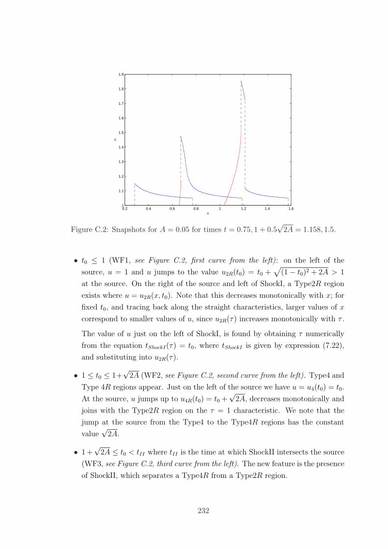
0.2 0.4 0.6 0.8 1 1.2 1.4 1.61
1.1
1.2
1.3
1.4
1.5
1.6
1.7
1.8
1.9
x
u
Figure C.2: Snapshots for A = 0.05 for times t = 0.75, 1 + 0.5√
2A = 1.158, 1.5.
• t0 ≤ 1 (WF1, see Figure C.2, first curve from the left): on the left of the
source, u = 1 and u jumps to the value u2R(t0) = t0 +√
(1− t0)2 + 2A > 1
at the source. On the right of the source and left of ShockI, a Type2R region
exists where u = u2R(x, t0). Note that this decreases monotonically with x; for
fixed t0, and tracing back along the straight characteristics, larger values of x
correspond to smaller values of u, since u2R(τ) increases monotonically with τ .
The value of u just on the left of ShockI, is found by obtaining τ numerically
from the equation tShockI(τ) = t0, where tShockI is given by expression (7.22),
and substituting into u2R(τ).
• 1 ≤ t0 ≤ 1+√
2A (WF2, see Figure C.2, second curve from the left). Type4 and
Type 4R regions appear. Just on the left of the source we have u = u4(t0) = t0.
At the source, u jumps up to u4R(t0) = t0 +√
2A, decreases monotonically and
joins with the Type2R region on the τ = 1 characteristic. We note that the
jump at the source from the Type4 to the Type4R regions has the constant
value√
2A.
• 1 +√
2A ≤ t0 < tII where tII is the time at which ShockII intersects the source
(WF3, see Figure C.2, third curve from the left). The new feature is the presence
of ShockII, which separates a Type4R from a Type2R region.
232
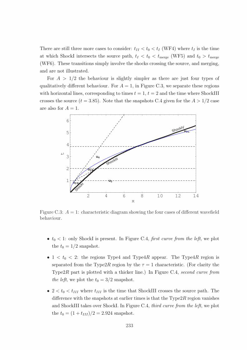
There are still three more cases to consider: tII < t0 < tI (WF4) where tI is the time
at which ShockI intersects the source path, tI < t0 < tmerge (WF5) and t0 > tmerge
(WF6). These transitions simply involve the shocks crossing the source, and merging,
and are not illustrated.
For A > 1/2 the behaviour is slightly simpler as there are just four types of
qualitatively different behaviour. For A = 1, in Figure C.3, we separate these regions
with horizontal lines, corresponding to times t = 1, t = 2 and the time where ShockIII
crosses the source (t = 3.85). Note that the snapshots C.4 given for the A > 1/2 case
are also for A = 1.
2 4 6 8 10 12 14x
1
2
3
4
5
6
t
Shock
I
ShockIII
ShockIV
u3
u3 L
u4 R
u4
u2 R
Figure C.3: A = 1: characteristic diagram showing the four cases of different wavefieldbehaviour.
• t0 < 1: only ShockI is present. In Figure C.4, first curve from the left, we plot
the t0 = 1/2 snapshot.
• 1 < t0 < 2: the regions Type4 and Type4R appear. The Type4R region is
separated from the Type2R region by the τ = 1 characteristic. (For clarity the
Type2R part is plotted with a thicker line.) In Figure C.4, second curve from
the left, we plot the t0 = 3/2 snapshot.
• 2 < t0 < tIII where tIII is the time that ShockIII crosses the source path. The
difference with the snapshots at earlier times is that the Type2R region vanishes
and ShockIII takes over ShockI. In Figure C.4, third curve from the left, we plot
the t0 = (1 + tIII)/2 = 2.924 snapshot.
233
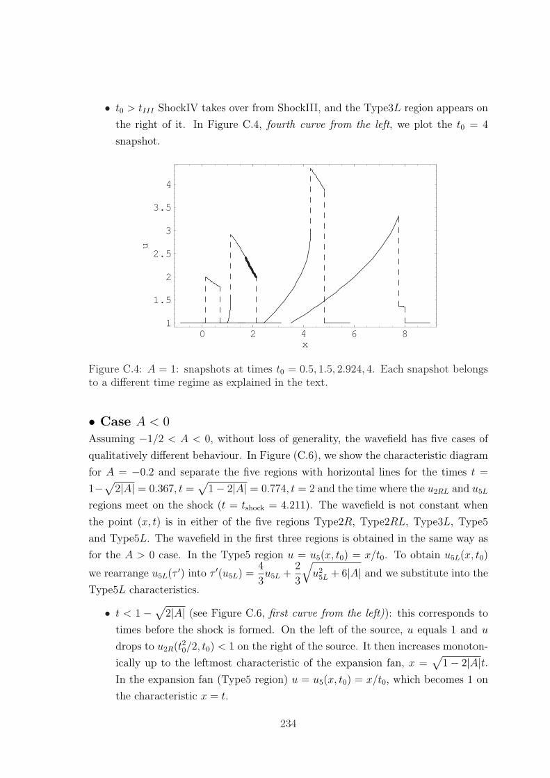
• t0 > tIII ShockIV takes over from ShockIII, and the Type3L region appears on
the right of it. In Figure C.4, fourth curve from the left, we plot the t0 = 4
snapshot.
0 2 4 6 8x
1
1.5
2
2.5
3
3.5
4
u
Figure C.4: A = 1: snapshots at times t0 = 0.5, 1.5, 2.924, 4. Each snapshot belongsto a different time regime as explained in the text.
• Case A < 0Assuming −1/2 < A < 0, without loss of generality, the wavefield has five cases of
qualitatively different behaviour. In Figure (C.6), we show the characteristic diagram
for A = −0.2 and separate the five regions with horizontal lines for the times t =
1−√
2|A| = 0.367, t =√
1− 2|A| = 0.774, t = 2 and the time where the u2RL and u5L
regions meet on the shock (t = tshock = 4.211). The wavefield is not constant when
the point (x, t) is in either of the five regions Type2R, Type2RL, Type3L, Type5
and Type5L. The wavefield in the first three regions is obtained in the same way as
for the A > 0 case. In the Type5 region u = u5(x, t0) = x/t0. To obtain u5L(x, t0)
we rearrange u5L(τ ′) into τ ′(u5L) =4
3u5L +
2
3
√u2
5L + 6|A| and we substitute into the
Type5L characteristics.
• t < 1 −√
2|A| (see Figure C.6, first curve from the left)): this corresponds to
times before the shock is formed. On the left of the source, u equals 1 and u
drops to u2R(t20/2, t0) < 1 on the right of the source. It then increases monoton-
ically up to the leftmost characteristic of the expansion fan, x =√
1− 2|A|t.In the expansion fan (Type5 region) u = u5(x, t0) = x/t0, which becomes 1 on
the characteristic x = t.
234
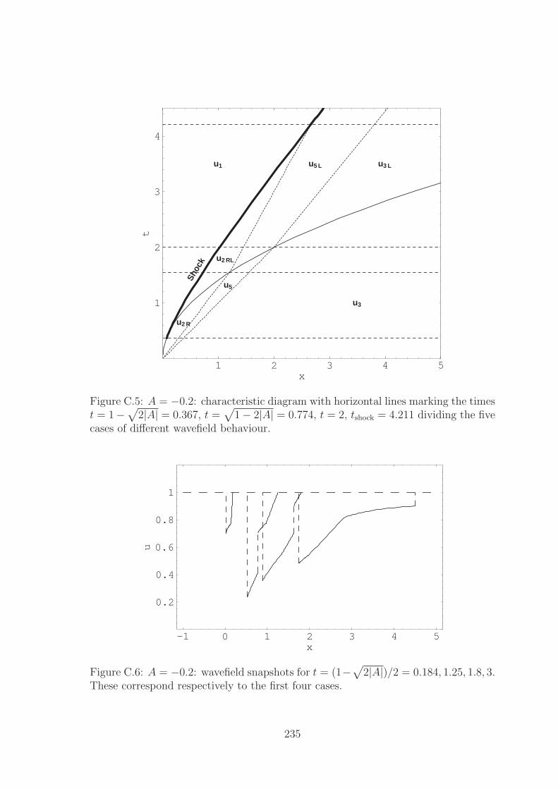
1 2 3 4 5x
1
2
3
4t
u3
u3 Lu1
u2 R
u2 RL
u5
u5 L
Shoc
k
Figure C.5: A = −0.2: characteristic diagram with horizontal lines marking the timest = 1−
√2|A| = 0.367, t =
√1− 2|A| = 0.774, t = 2, tshock = 4.211 dividing the five
cases of different wavefield behaviour.
-1 0 1 2 3 4 5x
0.2
0.4
0.6
0.8
1
u
Figure C.6: A = −0.2: wavefield snapshots for t = (1−√
2|A|)/2 = 0.184, 1.25, 1.8, 3.These correspond respectively to the first four cases.
235
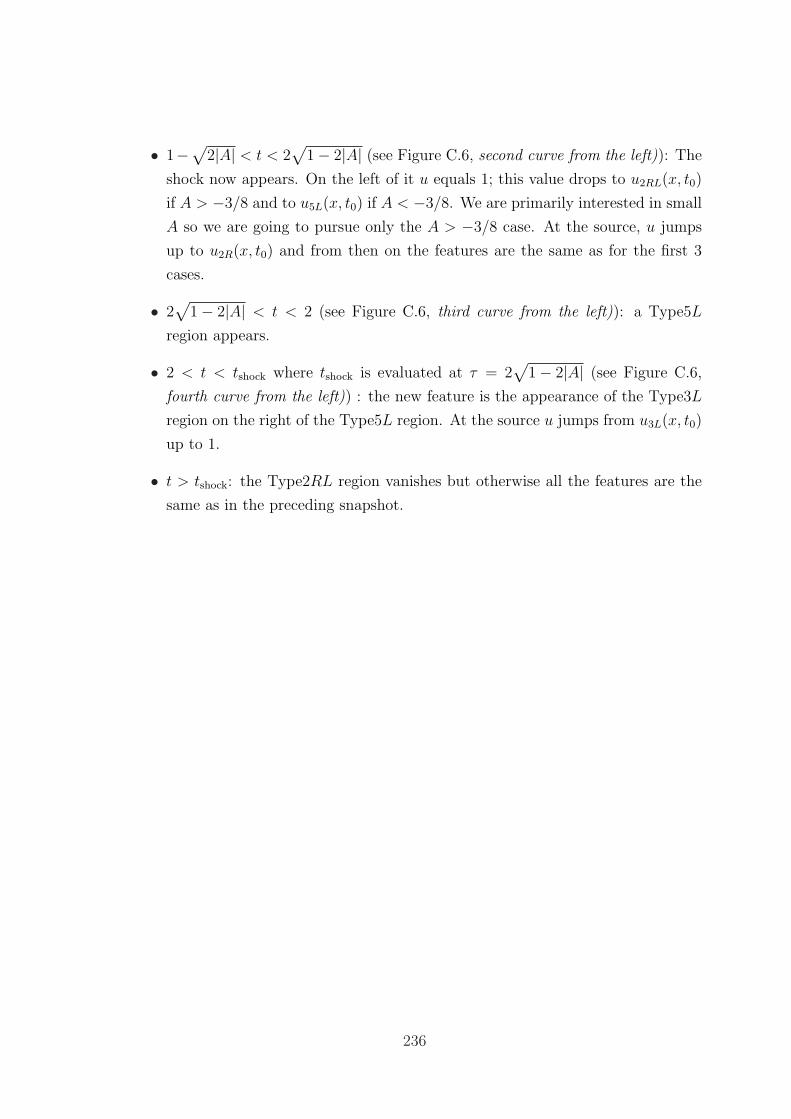
• 1−√
2|A| < t < 2√
1− 2|A| (see Figure C.6, second curve from the left)): The
shock now appears. On the left of it u equals 1; this value drops to u2RL(x, t0)
if A > −3/8 and to u5L(x, t0) if A < −3/8. We are primarily interested in small
A so we are going to pursue only the A > −3/8 case. At the source, u jumps
up to u2R(x, t0) and from then on the features are the same as for the first 3
cases.
• 2√
1− 2|A| < t < 2 (see Figure C.6, third curve from the left)): a Type5L
region appears.
• 2 < t < tshock where tshock is evaluated at τ = 2√
1− 2|A| (see Figure C.6,
fourth curve from the left)) : the new feature is the appearance of the Type3L
region on the right of the Type5L region. At the source u jumps from u3L(x, t0)
up to 1.
• t > tshock: the Type2RL region vanishes but otherwise all the features are the
same as in the preceding snapshot.
236
References
[1] M. Abramowitz and I.A. Stegun. Handbook of Mathematical Functions.
Wiley, New York, 1971.
[2] D.J. Acheson. Elementary Fluid Dynamics. Clarendon Press, Oxford, 1990.
[3] Federal Aviation Adminstration. Civil aircraft sonic boom. Aeronautics
and Space, Code of Federal Regulations, Title 14, Part 91, January 1987. pp.
169–170.
[4] G.B. Airy. On the intensity of light in the neighbourhood of a caustic. Trans.
Camb. Phil. Soc., 6:379–401, 1838.
[5] D.J. Allwright, L. Dallois, and K. Kaouri. SOBER report D9: Sec-
ondary sonic boom. Technical report, University of Oxford, July 2002.
[6] D.J. Allwright, L. Dallois, K. Kaouri, P. Blanc-Benon, J. Scott,
and U. Berger. SOBER report D14: Report and software code for simulat-
ing secondary boom in a three-dimensionally inhomogeneous atmosphere and
comparison with observations. Technical report, University of Oxford, Ecole
Centrale de Lyon, Leibniz-Institute of Atmospheric Physics, March 2004.
[7] D.J. Allwright, L. Dallois, K. Kaouri, P. Blanc-Benon, J. Scott,
and U. Berger. SOBER report D18: Guideline on the environmental impact
of secondary boom. Technical report, University of Oxford, Ecole Centrale de
Lyon, Leibniz-Institute of Atmospheric Physics, April 2004.
[8] D.J. Allwright and K. Kaouri. Circulation in inviscid gas flows with
shocks. Appl. Math. Let., 17:767–770, July 2004.
[9] T. Aubin and F. Coulouvrat. Nonlinear acoustic waves in a relaxing fluid.
J. Math. Pure Appl., 77(4):387, 1998.
237
[10] T. Auger. Modelisation et simulation numerique de la focalisation d’ondes
de chocs acoustiques en milieu en mouvement. Application a la focalisation du
bang sonique en acceleration. PhD thesis, Universite Paris VI, 2001.
[11] Th. Auger and F. Coulouvrat. Numerical simulation of sonic boom fo-
cusing. AIAA Journal, 40(9):1726–1734, 2002.
[12] H.E. Bass, J. Ezell, and R. Raspet. Effect of vibrational relaxation on rise
times of shock waves in the atmosphere. J. Acoust. Soc. Am., 74(5):1514–17,
1983.
[13] H.E. Bass, B.A. Layton, L.N. Bolen, and R. Raspet. Propagation of
medium strength shock waves through the atmosphere. J. Acoust. Soc. Am.,
82:306–310, 1987.
[14] G.K. Batchelor. An Introduction to Fluid Dynamics. Cambridge University
Press, 3rd edition, 2000.
[15] M.V. Berry. Waves and Thom’s theorem. Adv. Phys., 25:1–26, 1976.
[16] V. Bjerknes. On a fundamental theorem of hydrodynamics and its applica-
tions particularly to the mechanics of the atmosphere and the world’s oceans.
(in German). Proc. Roy. Swed. Acam. Sci., 1898.
[17] D.I. Blokhintsev. The propagation of sound in an inhomogeneous and mov-
ing medium I. J. Acoust. Soc. Am., 18:322–328, 1946.
[18] M. Born and E. Wolf. Principles of Optics. Cambridge University Press,
Cambridge, 7th edition, 2002.
[19] R.B. Buchal and Keller J.B. Boundary layer problems in diffraction
theory. Comm. Pur. Appl. Math., 13:85–144, 1960.
[20] L. Cambier. ”The elsA project”. In First ONERA/DLR Aerospace Sympo-
sium, Paris, June 1999.
[21] C. J Chapman. High Speed Flow. Cambridge University Press, 2000.
[22] C.J. Chapman. Time-domain asymptotics and the method of stationary phase.
Proc. Roy. Soc. Lon., 437(1899):25–40, 1992.
238
[23] H.K. Cheng and M.M. Hafez. The superboom as a Tricomi problem: appli-
cation. In IUTAM Symposium Transsonicum, Gottingen, Germany, September
2002.
[24] R. Cleveland. Propagation of sonic booms through a real, stratified atmo-
sphere. PhD thesis, Univ. Texas at Austin., 1995.
[25] F. Coulouvrat. Focusing of weak acoustic shock waves at a caustic cusp.
Wave Motion, 32(3):233–45, 2000.
[26] F. Coulouvrat. Sonic boom in the shadow zone: a geometrical theory of
diffraction. J. Acoust. Soc. Am., 111(1):499–508, 2001.
[27] F. Coulouvrat. Numerical simulation of shock wave focusing at fold caustics
with application to sonic boom. J. Acoust. Soc. Am., 114(4):1758–1771, 2003.
[28] M.S. Cramer. Focusing of weak three-dimensional shock waves. AIAA Jour-
nal, 19(10):1363–1365, 1981.
[29] M.S. Cramer and A.R. Seebass. Focusing of weak shock waves at an arete.
J. Fluid Mech., 110:249–253, 1981.
[30] S.C. Crow. Distortion of sonic bangs by atmospheric turbulence. J. Fluid
Mech., 37:529–563, 1969.
[31] L. Dallois, P. Blanc-Benon, J. Scott, U. Berger, D.J. Allwright,
and K. Kaouri. Secondary sonic boom modelling for realistic atmospheric
conditions. In Proceedings of the CFA-DAGA Meeting, Strasburg, 2004.
[32] D.F. Dempsey. Focusing conditions for sonic booms. J. Acoust. Soc. Am.,
61(3), March 1977.
[33] W.L. Donn. Exploring the atmosphere with sonic booms. American Scientist,
66:724–733, 1978.
[34] M. Downing, N. Zamot, C. Moss, D. Morin, Ed. Wolski, S. Chung,
K. Plotkin, and D. Maglieri. Controlled focused sonic booms from ma-
neuveuring aircraft. J. Acoust. Soc. Am., 104(1), 1998.
[35] J.W.M. DuMond, E.R. Cohen, W.K.H. Panofksy, and E. Deeds. A
determination of the wave forms and laws of propagation and dissipation of
ballistic shock waves. J. Acoust. Soc. Am., 18(1):97–118, 1946.
239
[36] Effects of aircraft noise and sonic boom on domestic animals and wildlife: A
literature synthesis. Engineering and Services Centre, Fish and Wildlife Service,
U.S. Air Force, June 1988.
[37] T.P. Evans and J.J. Doherty. The aerodynamic design of EUROSUP
configuration. DERA/AS/ASD/CR97620/1.0, 1997.
[38] A. Ferri, L. Ting, and R.W. Lo. Nonlinear sonic boom propagation in-
cluding the asymmetric effects. AIAA Journal, 15(5):653–658, 1977.
[39] F.I. Frankl and E.A. Karpovich. Gas Dynamics of Thin Bodies. Inter-
science Publishers Ltd., 1953.
[40] F. G. Friedlander. Sound Pulses. Cambridge University Press, 1958.
[41] K.Y. Fung. Shock wave formation at a caustic. SIAM J. Appl. Math., 39:355–
371, 1980.
[42] G. Gilbert and H.E.H. Davies. Pantograph motion on a nearly uniform
railway overhead line. Proc. IEE, 113(3):485–492, 1966.
[43] P.M. Gill and A.R. Seebass. Nonlinear acoustic behavior at a caustic:
an approximate analytical solution. In AIAA Aeroacoustics Conference, Cam-
bridge, MA, U.S.A., 1973. MIT Press.
[44] M.E. Goldstein. Aeroacoustics. McGraw-Hill International Book Co, New
York, 1976.
[45] J.-P. Guiraud. Acoustique geometrique, bruit balistique des avions superson-
iques et focalisation. J. Mec., 4:215–267, 1965.
[46] J. Hadamard. Lecons sur la Propagation de Ondes. Hermann, Paris, 1903.
[47] G.T. Haglund and E.J. Kane. Analysis of sonic boom measurements near
shock wave extremities for flight near Mach 1.0 and for airplane accelerations.
NASA CR, 2417, 1974.
[48] G.T. Haglund and H.W. Poling. HSCT sonic boom impact at the Earth’s
surface due to secondary booms. Technical report, Boeing Commercial Airplane
Company, Seattle, WA, 1995. Prepared for Nasa Langley Research Center,
contract NAS1-20220.
240
[49] P.W. Hammerton. Effect of molecular relaxation on the propagation of sonic
booms through a stratified atmosphere. Wave Motion, 33(4):359–377, April
2001.
[50] W.D. Hayes. Linearised Supersonic Flow. PhD thesis, California Institute of
Technology, 1947.
[51] W.D. Hayes. Pseudotransonic similitude and first-order wave structure. J.
Aero. Sci., 21:721–730, 1954.
[52] W.D. Hayes. Brief review of the basic theory: sonic boom research. NASA
SP, 147:3–7, 1967.
[53] W.D. Hayes. Similarity rules for nonlinear acoustic propagation through a
caustic. (Proceedings of the second conference on sonic boom research). NASA
SP, 180:165–171, 1967.
[54] W.D. Hayes, R.C. Haefeli, and H.E. Kulsrud. Sonic boom propagation
in a stratified atmosphere, with computer program. NASA CR, 1299, 1969.
[55] H.M. Helfand. An application of the method of Multiple Scales to problems
arising in supersonic aerodynamics and stratified fluid mechanics. PhD thesis,
Cornell University, 1974.
[56] G.S. Heller. Propagation of acoustic discontinuities in an inhomogeneous
moving liquid medium. J. Acoust. Soc. Am., 25:950–951, 1953.
[57] A.L. Hoffman. A single fluid model for shock formation in MHD shock tubes.
J. Plasma Phys., 1:193–207, 1967.
[58] H. Huang. Private communication. York University, Toronto, Canada.
[59] J.K. Hunter and J.B. Keller. Caustics of nonlinear waves. Wave Motion,
9(5):429–443, 1987.
[60] J Jena and V.D. Sharma. Far-field behaviour of waves in a relaxing gas.
Acta Astronautica, 40(10):713–718, 1996.
[61] C.N. Jensen. Nonlinear systems with discrete and continuous elements. PhD
thesis, Technical University of Denmark, 1997.
241
[62] M.E. Johnson and P.W. Hammerton. Effect of molecular relaxation pro-
cesses on travelling wave solutions of sonic boom waveforms. Wave Motion,
38(3):229–240, September 2003.
[63] K. Kaouri. Effects of the earth’s curvature and rotation on sound ray propa-
gation. Technical report, OCIAM, Mathematical Institute, Oxford., 2002.
[64] K. Kaouri. Solution of the kinematic wave equation with an accelerating point
source. Wave Motion, 2004. (in press).
[65] J.B. Keller. Geometrical acoustics I: the theory of weak shock waves. J.
Appl. Phys., 25(8):938–947, 1954.
[66] J.B. Keller. A geometrical theory of diffraction. In Proc. Symposia Appl.
Math., 8, pages 27–32. McGraw-Hill, 1958.
[67] L.D. Landau. On shock waves at large distances from the place of their origin.
Journal of Physics of the Academy of Sciences of the U.S.S.R., 9:496, 1945.
[68] J.M. Lawry. Some results on diffraction theory. Master’s thesis, Oxford
University, 1993.
[69] R.J. LeVeque. Finite Volume Methods for Hyperbolic Problems. Cambridge
University Press, Cambridge, 2002.
[70] H.W. Liepmann and A. Roshko. Elements of Gasdynamics. John Wiley,
Inc., 1956.
[71] M.J. Lighthill. The conditions behind the trailing edge of the supersonic
aerofoil. Rep. Memor. Aero. Res. Comm. Lond., 1930, 1944.
[72] M.J. Lighthill. Waves in Fluids. Cambridge University Press, 1978.
[73] G.M. Lilley, R. Westley, A.H. Yates, and J.R. Busing. Some aspects
of noise from supersonic aircraft. J. Roy. Aero Soc., 57:396–414, 1953.
[74] H. Lomax. The wave drag of arbitrary configurations in linearised flow as
determined by areas and forces in oblique planes. NACA RM, A55 A18, 1955.
[75] D. Ludwig. Uniform asymptotic expansions at a caustic. Comm. Pur. Appl.
Math., 19:215–250, 1966.
242
[76] D.J. Maglieri and K.J. Plotkin. Sonic Boom, chapter 10, pages 519–561.
NASA, USA, 1991.
[77] R. Marchiano, F. Coulouvrat, and Grenon R. Numerical simulation of
shock wave focusing at fold caustics, with application to sonic boom. J. Acoust.
Soc. Am., 114(4):1–14, 2003.
[78] R. Marchiano, F. Coulouvrat, and J.-L. Thomas. Focusing of finite
amplitude waves at caustics. Moscow (Russia), August 2002. 16th Int. Sump.
Nonlinear Acoustics.
[79] D.A. McCurdy, S.A. Brown, and R.D. Hilliard. The effects of simulated
sonic booms on people in their homes. In 33rd Aerospace Sciences Meeting,
AIAA, 95-0834, 1995.
[80] C.B. Moler and L.P. Solomon. Use of splines and numerical integration
in Geometrical Acoustics. J. Acoust. Soc. Am., 48:739–734, 1970.
[81] J.F. Nye. Natural focusing and fine structure of light: caustics and wave
dislocations. Institute of Physics Publishing, Bristol, 1999.
[82] H. Ockendon and J.R. Ockendon. Waves and Compressible Flow.
Springer-Verlag, New York; London, 2004.
[83] H. Ockendon and D.A. Spence. Nonlinear wave propagation in a relaxing
gas. J. Fluid Mech., 39:329–345, 1969.
[84] H. Ockendon and A.B. Tayler. Inviscid Fluid Flows. Springer-Verlag,
New York, 1983.
[85] J. Ockendon, S. Howison, A. Lacey, and A. Movchan. Applied Partial
Differential Equations. Oxford University Press, 1st edition, 1999.
[86] J. Ockendon, S. Howison, A. Lacey, and A. Movchan. Applied Partial
Differential Equations. Oxford University Press, 2nd edition, 2003.
[87] C. B. Officer. Introduction to the Theory of Sound Transmission: With Ap-
plication to the Ocean. McGraw-Hill series in the geological sciences. McGraw-
Hill, 1958.
[88] R.O. Onyeowu. Diffraction of sonic boom past the nominal edge of the
corridor. J. Acoust. Soc. Am., 58:326–330, 1975.
243
[89] N.W. Page and K.J. Plotkin. An efficient method for incorporating Com-
putational Fluid Dynamics into sonic boom prediction. AIAA-1991, page
3275. AIAA Aeroacoustics conference, 1991.
[90] T. Pearcey. The structure of an electromagnetic field in the neighbourhood
of a cusp of a caustic. Phil. Mag., 37:311–7, 1946.
[91] W.R. Pechuzal and J. Kevorkian. Supersonic-transonic flow generated
by a thin airfoil in a stratified atmosphere. SIAM J. Appl. Math., 33(1):8–33,
1977.
[92] A.D. Pierce. Maximum overpressures of sonic boom near the cusp of caustic.
In M.J. Crocker, editor, Noise and Vibration Control Engineering., pages
478–487. Purdue University Press, 1971.
[93] A.D. Pierce. Statistical theory of atmospheric turbulence on sonic boom rise
times. J. Acoust. Soc. Am., 49:906–924, 1971.
[94] A.D. Pierce. Acoustics, an Introduction to its Physical Principles and Appli-
cations. Acoustical Society of America, 1994.
[95] A.D. Pierce. Dispersion relation influence on rise times of sonic boom prop-
agation through turbulence. J. Acoust. Soc. Am., 99(4):2488–2500, 1996.
[96] A.D. Pierce and D.J. Maglieri. Effects of atmospheric irregularities on
sonic boom propagation. J. Acoust. Soc. Am., 51(2):702–721, 1972.
[97] K.J. Plotkin. Sonic boom focal zones from tactical aircraft maneuvers. J.
Aircraft, 30(1):75–80, 1993. interlibrary.
[98] K.J. Plotkin. State of the art of sonic boom modeling. J. Acoust. Soc. Am.,
104:1830, 1998.
[99] K.J. Plotkin. State of the art of sonic boom modeling. J. Acoust. Soc. Am.,
111(1):530–536, 2002.
[100] K.J. Plotkin and N.W. Page. Extrapolation of sonic boom signatures from
CFD solutions. AIAA-0922, pages 1–6. AIAA Aeroacoustics conference, 2002.
[101] A.L. Polyakova, S.I. Soluyan, and R.V. Khokhlov. Propagation of
finite disturbances in a relaxing medium. Soviet Phys. Acoust., 8:78–82, 1962.
244
[102] P.S. Rao. Supersonic bangs I. Aero Q., 7:21–44, 1956.
[103] P.S. Rao. Supersonic bangs II. Aero Q., 7:135–155, 1956.
[104] E. Rickley and A. Pierce. Detection and assessment of secondary sonic
booms in New England. J. Acoust. Soc. Am., 67(1), 1980.
[105] R. A. Riehle and R.C. Newman, editors. Principles of Extracorporeal Shock
Wave Lithotripsy. Churchill Livingstone, New York, 1987.
[106] L.D. Robinson. Sonic boom propagation through an inhomogeneous, windy
atmosphere. PhD thesis, University of Texas at Austin., 1991.
[107] R Rodeman, D.B. Longcope, and L.F Shampine. Response of a string
to an accelerating mass. J. Applied Mech., 98(4):675–680, 1976.
[108] P.H. Rogers and J.H. Gardner. Propagation of sonic booms in the ther-
mosphere. J. Acoust. Soc. Am., 67(1):79–91, 1980.
[109] R.R. Rosales and E.G. Tabak. Caustics of weak shock waves. Phys. Fluids,
10(1):206–222, 1998.
[110] C. Schar. Infrasonic wave propagation in the atmosphere (in German)., 1993.
[111] J. Scott. personal communication.
[112] W.R. Sears, editor. General Theory of High Speed Aerodynamics. Princeton
University Press, 1954.
[113] A.R. Seebass. Nonlinear acoustic behavior at a caustic. (Proceedings of the
third conference on sonic boom research.). NASA SP, 255:87–120, 1971.
[114] K.P. Shepherd, S.A. Brown, J.D. Leatherwood, and D.A. McCurdy.
Human response to sonic booms-recent NASA research. NASA Langley Re-
search Center, Hampton, VA 23681, USA.
[115] Y.L. Sinai and J.F. Clarke. The wave system attached to a finite slender
body in a supersonic relaxing gas stream. J. Fluid Mech., 84:717–741, 1978.
[116] M.J.T. Smith. Aircraft Noise. Cambridge University Press, 1989.
[117] V. Sparrow. Review and status of sonic boom penetration into the ocean. J.
Acoust. Soc. Am., 111(1):537–543, 2002.
245
[118] B. Sturtevant and V.A. Kulkarny. The focusing of weak shock waves.
J. Fluid Mech., 73(4):651–671, 1976.
[119] A.D. Taylor. The TRAPS sonic boom program. Technical report, U.S. Dept.
of Commerce, 1980.
[120] C.L. Thomas. Extrapolation of sonic boom pressure signatures by the wave-
form parameter method. NASA TN, D-6832, 1972.
[121] M.D. Van Dyke. Perturbation Methods in Fluid Mechanics. Stanford:
Parabolic Press, 1975.
[122] F. Walkden. The shock pattern of a wing-body combination, far from the
flight path. Aeronautical Q., IX:164–194, 1958.
[123] J.-C.L. Wanner, J. Vallee, C. Vivier, and C. Thery. Theoretical and
experimental studies of the focus of sonic booms. J. Acoust. Soc. Am., 52(1):13–
32, 1972.
[124] G.B. Whitham. The flow pattern of a supersonic projectile. Comm. Pur.
Appl. Math., 5:301–348, 1952.
[125] G.B. Whitham. On the propagation of weak shocks. J. Fluid Mech., 1:290–
318, 1956.
[126] G.B. Whitham. Linear and Nonlinear Waves. Wiley, New York, 1974.
246


![VARIABILITY OF MEASURED SONIC BOOM ... CONTRACTOR REPORT 191483 VARIABILITY OF MEASURED SONIC BOOM SIGNATURES VOLUME I - TECHNICAL REPORT K. 1L ELMER M.C. JOSH] MCDONNELL DOUGLAS AEROSPACE](https://img.pdfslide.us/doc/110x75/5abcbc457f8b9a567c8e245f/variability-of-measured-sonic-boom-contractor-report-191483-variability-of-measured.jpg)