Embed Size (px)
Citation preview
Generated using version 3.1.2 of the official AMS LATEX template
Secondary instabilities in breaking inertia-gravity waves
Mark D. Fruman ∗ and Ulrich Achatz
Institute for Atmospheric and Environmental Sciences, Goethe University Frankfurt, Germany
∗Corresponding author address: M. D. Fruman, IAU, Goethe Universitat-Frankfurt, Altenhoferallee 1,
60438 Frankfurt am Main, Germany.
E-mail: [email protected]
1
ABSTRACT
The three-dimensionalization of turbulence in the breaking of nearly vertically propagat-
ing inertia-gravity waves is investigated numerically using singular vector analysis applied
to the Boussinesq equations linearized about three two-dimensional time-dependent basic
states obtained from nonlinear simulations of breaking waves: a statically unstable wave
perturbed by its leading transverse normal mode, the same wave perturbed by its leading
parallel normal mode, and a statically stable wave perturbed by a leading transverse singular
vector. The secondary instabilities grow through interaction with the buoyancy gradient and
velocity shear in the basic state. Which growth mechanism predominates depends on the
time dependent structure of the basic state and the wavelength of the secondary perturba-
tion. The singular vectors are compared to integrations of the linear model using random
initial conditions, and the leading few singular vectors are found to be representative of the
structures that emerge in the randomly initialized integrations. A main result is that the
length scales of the leading secondary instabilities are an order of magnitude smaller than
the wavelength of the initial wave, suggesting that the essential dynamics of the breaking
might be captured by tractable nonlinear three-dimensional simulations in a relatively small
triply periodic domain.
1. Introduction
The importance of gravity waves to the large scale circulation in the middle atmosphere
is well established. The mean state of the atmosphere as well as phenomena such as the cold
summer pole in the mesopause (Houghton 1978) and the quasi-biennial oscillation (QBO) in
equatorial winds in the stratosphere (Lindzen and Holton 1968) cannot be properly explained
without accounting for the effects of gravity waves.
The range of scales inherent in the sources of gravity waves in the middle atmosphere,
especially flow over topography and convection but also spontaneous emission from the
1
adjustment of balanced flows, is reflected in the range of temporal and spatial scales involved,
from minutes to several hours and tens of metres to thousands of kilometres (see Fritts et al.
2006, for a review of the characteristics of gravity wave sources). Due to the range of scales
involved, both the sources of gravity waves and the momentum deposition associated with
their breaking, known as gravity-wave drag, must be at least partially parameterized in
general circulation models.
Most parameterization schemes, such as that of Lindzen (1981) and Holton (1982), are
based on the criterion of static instability (also known as convective instability). Gravity
waves from a source with prescribed wavenumber and frequency spectrum are assumed to
propagate vertically against a mean background wind and temperature field. The propaga-
tion of the waves is assumed to follow the predictions of WKBJ theory (Bretherton 1966;
Grimshaw 1975; Muller 1976), wherein the frequency, vertical wavenumber and amplitude
of the waves vary depending on the structure of the background fields. At the point at
which the waves become statically unstable, i.e. where the total potential temperature field
decreases locally with height, some or all of the momentum of the waves is absorbed by the
mean flow and the amplitude of the waves as they continue upward is reduced relative to the
growth predicted by linear theory. See McLandress (1998) and Fritts and Alexander (2003)
for reviews of gravity wave parameterization and surveys of commonly used schemes.
Since there is great uncertainty in all aspects of gravity wave modeling, parameterizations
can be tuned extensively in order to produce a realistic forcing on the circulation. Ultimately,
in order for progress to be made in parameterizing gravity-wave breaking, for example with
a view to simulating future climate scenarios, it is of primary importance to understand the
conditions under which a wave will break as well as the detailed dynamics of the breaking.
Mied (1976) and Drazin (1977) showed using Floquet theory that inviscid monochromatic
gravity waves are linearly unstable at all amplitudes even if their amplitudes are far from the
threshold for static instability and their Richardson numbers greater than 1/4, the sufficient
condition for stability of a steady shear flow (Miles 1961; Howard 1961). Later, Klostermeyer
2
(1983) showed how weak viscosity affects the growth rates and spatial scales of the leading
unstable modes, a relevant point since in the mesosphere the kinematic viscosity and thermal
diffusivity are relatively large due to the very low ambient density.
The above studies neglect the effect of rotation, which becomes significant for steeply
propagating waves, so-called inertia-gravity waves (IGW). Due to their very low frequencies
and near horizontal symmetry, steeply propagating waves can be modeled to a large extent
as steady stratified shear flows, whereby Dunkerton (1997) and Achatz and Schmitz (2006)
obtained approximate analytic results. These studies and numerical studies by Yau et al.
(2004), Lelong and Dunkerton (1998a,b), and Achatz (2005) found that rotation strongly af-
fects the orientation of the most unstable perturbations relative to the propagation direction
of the wave. This is because waves affected by rotation have a nonzero velocity component
in the direction perpendicular to the plane of the wave. It has also been shown that shear
instability occurs in IGW below the threshold for static instability.
Most numerical studies of gravity wave breaking have considered only two-dimensional
breaking, but the fact that there are linearly unstable perturbations with all orientations
relative to the propagation direction of the wave indicates that in practice the process must
be strongly three dimensional. Nonlinear numerical simulations by Andreassen et al. (1994)
(see also Fritts et al. 1994) of breaking high-frequency gravity waves found fundamentally
different behaviour in two- and three-dimensional simulations, with more efficient reduc-
tion of the amplitude of the gravity wave and generation of turbulence occurring in the
three-dimensional simulations. More recently, Fritts et al. (2009a,b) used simulations at
much higher resolution and with higher Reynolds numbers more realistic for the atmosphere
and again found differences between the two- and three-dimensional dynamics. Initially,
two-dimensional structures on the scale of the initial wave dominate, while later on, local
instabilities lead to the formation of small scale three-dimensional structures. Another im-
portant point is that waves with amplitudes both above and below the threshold for static
instability break, but the relative sizes of the buoyancy and momentum flux differ depending
3
on the static stability of the wave.
There have been to our knowledge no three-dimensional direct numerical simulations
(DNS), comparable to those of Fritts et al. (2009a,b), of breaking IGW (meaning waves
affected by rotation) with parameters realistic for the middle atmosphere and of high enough
resolution to reliably represent the small scales that emerge in the turbulent evolution of the
breaking wave. This is partly because of their very long horizontal scale, a difficulty that
may be overcome by a change of reference frame (as explained below) or by artificially
reducing the ratio N/f (Lelong and Dunkerton 1998a,b), and partly due to the fact that
since the vertical momentum flux associated with a gravity wave decreases with decreasing
intrinsic frequency (Fritts et al. 2006) there has been less interest in IGW breaking than
in the breaking of high frequency waves. That is not to say, however, that the cumulative
effect of IGW on the large scale circulation is negligible. A recent observational case study by
Nicolls et al. (2010) found that a breaking IGW with properties similar to those considered
here accelerated the background flow by 10-20 ms−1.
Three-dimensional simulations are of course computationally expensive, especially given
the scales of low-frequency inertia-gravity waves, and are thus impractical for investigating
much of parameter space. However, since for related problems three-dimensional simula-
tions have indicated essential differences in the two- and three-dimensional aspects of wave
breaking, including different temporal and spatial scales, the following three-stage approach
presents itself. First, the leading primary linear instabilities of the IGW are computed. Next,
high resolution nonlinear two-dimensional simulations initialized with the superposition of
the IGW and its leading linear modes are performed. Finally the linear stability, with re-
spect to perturbations varying in the remaining spatial direction, of the two-dimensional
time dependent states obtained from the nonlinear integrations is considered. The latter is
a two-dimensional problem because the coefficients in the linearized equations depend only
on two spatial dimensions, and is the subject of the present article.
The idea of analyzing the linear stability of numerically calculated two-dimensional non-
4
linear solutions to perturbations varying in the perpendicular direction was used by Klaassen
and Peltier (1985a,b) for the problem of Kelvin-Helmholtz instability. Assuming the growth
of the secondary instabilities is much faster than the evolution of the two-dimensional basic
state, they took the two-dimensional state to be time-independent. The resulting linearized
equations could then be analyzed in terms of normal modes. The effect of the temporal evo-
lution of the basic state was considered by performing the linearization at different times.
Here we investigate secondary instabilities using singular vector analysis (Farrell and Ioan-
nou 1996a,b), whereby the perturbations whose energy grows by the largest factor within a
given optimization time are computed. Unlike normal mode analysis, singular vectors may
be computed even for time dependent basic states. In addition, even when the system is
non-normal, singular vectors are the eigenvectors of a real, symmetric matrix and thus form
an orthogonal set, both at the initial time and at the optimization time, making it possible
to project an arbitrary state onto a subset of the leading singular vectors without comput-
ing the whole set. Disadvantages of singular vector analysis are that the singular vectors
have time dependent spatial structure and are thus difficult to compare to, say, observed
structures (although it can identify temporal and spatial scales which one may compare with
observations) and that it cannot distinguish between true linearly unstable, exponentially
growing modes, and the transient growth of a linear combination of oscillatory modes. On
the other hand, with respect to the latter point, if perturbations are finite amplitude, modes
with large transient growth can be the most interesting in practice, leading to nonlinear
effects which dominate the subsequent evolution.
The determination of the primary linear instabilities and the nonlinear two-dimensional
integrations are the subjects of Achatz and Schmitz (2006) and Achatz (2007) respectively.
To describe the orientation of the primary perturbations, we adopt the terminology of
Dunkerton (1997): perturbations varying in the direction perpendicular to the plane of the
wave are called transverse, and perturbations varying in the plane of the wave are called par-
allel. In the present article we focus on two cases identified by Achatz (2007) as particularly
5

effective in reducing the amplitude of the initial IGW. In both cases the wave propagates in
the x-z plane with an angle of phase propagation of 89.5 to the horizontal and a vertical
wavelength of 6 km. In the first case the IGW is statically unstable, with amplitude 1.2 times
the threshold amplitude for static instability, and the primary perturbation is the leading
transverse normal mode (varying in the y direction). The second case is a statically stable
wave with non-dimensional amplitude 0.86 perturbed by a leading transverse singular vector.
We also investigate the secondary instabilities of the statically unstable IGW perturbed by
its leading parallel normal mode, which is the fast growing of all the normal modes.
The paper is organized as follows: In section 2, the Boussinesq equations in a coordinate
system moving with the wave and rotated so that one axis is parallel to the wavevector of
the IGW, as well as the properties of the IGW solution itself, are reviewed and the hierarchy
of IGW, primary perturbations and secondary perturbations introduced. Section 3 is a
brief outline of singular vector analysis. Section 4 describes the primary instabilities of the
IGW and the basic states taken from Achatz (2007), and Section 5 discusses the secondary
instabilities in terms of singular vectors.
2. Governing equations, the inertia-gravity wave solu-
tion, and primary and secondary perturbations
We use the Boussinesq equations on an f plane,
Du
Dt− fv +
∂P
∂x= ν∇2u, (1a)
Dv
Dt+ fu+
∂P
∂y= ν∇2v, (1b)
Dw
Dt− b+
∂P
∂z= ν∇2w, (1c)
Db
Dt+N2w = µ∇2b, (1d)
∂u
∂x+
∂v
∂y+
∂w
∂z= 0, (1e)
6
where v = (u, v, w) is the velocity field, buoyancy b is defined in terms of potential tem-
perature θ by b ≡ (θ − θ)/θ0, where θ(z) is the background potential temperature and θ0
a representative constant value, N2 ≡ (g/θ0)dθ/dz is the square of the Brunt-Vaisala fre-
quency, f ≡ 2Ω sinφ0 is the Coriolis parameter at a reference latitude φ0, ν is the kinematic
viscosity, and µ the thermal diffusivity. In all simulations, a value of 1 m2 s−1, typical of the
mesopause region, was used for both ν and µ, N was constant and equal to 2 × 10⁻² s−1,
and the f -plane was centred at φ0 = 70N. The material time derivative is defined by
D
Dt≡ ∂
∂t+ v · ∇. (2)
In the absence of dissipation (ν = µ = 0)1, a monochromatic inertia-gravity wave is an
exact solution to (1) of the form
[u, v, w, b] = Re
[u, v, w, b] exp [i(kx+mz − ωt)]
, (3)
where hatted variables are complex constants, and the constants k and m are the horizontal
and vertical wavenumbers, related to the frequency ω through the dispersion relation
ω2 = N2 cos2 Θ+ f 2 sin2 Θ, (4)
where Θ = tan−1(m/k) is the angle of phase propagation of the wave relative to the hori-
zontal. Since f and N do not depend on horizontal position, there is no preferred horizontal
direction and no loss of generality in considering a wave with wavevector in the x-z plane.
The complex amplitudes satisfy the polarization relations
[u, v, w, b] = a
[
ω
k,−i
f
k,− ω
m, iN2
m
]
, (5)
where a is a dimensionless constant defined so that a = 1 corresponds to a wave neutral with
respect to static stability at its least stable point. Notice that because of the Coriolis force,
the horizontal component of the velocity vector rotates with time.
1In the dissipative case, if µ = ν (Prandtl number unity), then (3) is still a solution, but with amplitude
decaying with time.
7
As mentioned, the problem of gravity wave stability is greatly simplified by working in a
Cartesian coordinate system rotated about the y axis so that the vertical axis is parallel to
the wave-vector of the wave (Mied 1976). Let the new coordinates be (ξ, y, ζ), where
ξ = sinΘ x− cosΘ z, (6a)
ζ = cosΘ x+ sinΘ z, (6b)
with associated velocity components uξ, v and wζ .
Written in terms of ξ, y, φ and t, where φ = Kζ − ωt is the phase of the wave and
K ≡√k2 +m2, the system (1) becomes
Duξ
Dt− f sinΘ v +
∂p
∂ξ+ cosΘ b = ν∇2uξ, (7a)
Dv
Dt+ f(sinΘ uξ + cosΘ wζ) +
∂p
∂y= ν∇2v, (7b)
Dwζ
Dt− f cosΘ v +K
∂p
∂φ− sinΘ b = ν∇2wζ , (7c)
Db
Dt+N2(− cosΘ uξ + sinΘ wζ) = µ∇2b, (7d)
∂uξ
∂ξ+
∂v
∂y+K
∂wζ
∂φ= 0, (7e)
where now
D
Dt≡ ∂
∂t+ uξ
∂
∂ξ+ v
∂
∂y+ (Kwζ − ω)
∂
∂φ, (8)
and the gravity wave solution (3) becomes
uξ = U(0)ξ = −
√K2ω
kmsinφ, (9a)
v = V (0) =f
kcosφ, (9b)
wζ = W(0)ζ = 0, (9c)
b = B(0) = −N2
mcosφ. (9d)
Using φ as coordinate in place of ζ places us in the reference frame moving with the phase
velocity of the gravity wave.
8
The instability analysis proceeds by linearizing (7) about the solution (9) and looking for
growing perturbations. Because the gravity wave is independent of ξ and y, perturbation
solutions exist of the form
[u′(p)ξ , v
′(p), w′(p)ζ , b
′(p)] = Re
[u′(p)ξ (φ, t), v
′(p)(φ, t), w′(p)ζ (φ, t), b
′(p)(φ, t)] exp [i(kξξ + kyy)]
,
(10)
which we refer to as primary perturbations. While it may be unstable to three-dimensional
perturbations, if not perturbed a nonlinear integration initialized with an IGW and one
of its leading unstable primary perturbations remains two-dimensional in space, with all
fields depending on only the IGW phase φ and the spatial coordinate in the direction of the
wavevector (kξ, ky) of the primary perturbation. It is therefore convenient to introduce an
additional coordinate transformation
x‖ = cosα ξ + sinα y, (11a)
y⊥ = − sinα ξ + cosα y, (11b)
where α ≡ tan−1(ky/kξ), and the corresponding velocity components u‖ and v⊥. For parallel
primary perturbations u‖ = uξ and v⊥ = v, and for transverse primary perturbations u‖ = v
and v⊥ = −uξ.
We investigate the three-dimensionalization of the turbulence that develops in the break-
ing of an inertia-gravity wave by linearizing (7) about the time-dependent nonlinear devel-
opment of the state initialized with the IGW and a leading primary perturbation, referred
to henceforth as the time-dependent basic state,
[u‖, v⊥, wζ , b] =[
U‖(x‖, φ, t), V⊥(x‖, φ, t),Wζ(x‖, φ, t), B(x‖, φ, t)]
, (12)
9
yielding
D′u′‖
Dt+
∂U‖
∂x‖
u′‖ +K
∂U‖
∂φw′
ζ − f(sinΘ v′⊥ + sinα cosΘ u′‖) +
∂p′
∂x‖
+ cosα cosΘ b′ = ν∇2u′‖,
(13a)
D′v′⊥Dt
+∂V⊥
∂x‖
u′‖ +K
∂V⊥
∂φw′
ζ + f(sinΘ u′‖ + cosα cosΘ w′
ζ) +∂p′
∂y⊥− sinα cosΘ b′ = ν∇2v′⊥,
(13b)
D′w′ζ
Dt+
∂Wζ
∂x‖
u′‖ +K
∂Wζ
∂φw′
ζ − f(sinα cosΘ u′‖ + cosα cosΘ v′⊥) +K
∂p′
∂φ− sinΘ b′ = ν∇2w′
ζ ,
(13c)
D′b′
Dt+N2(− cosα cosΘ u′
‖ + sinα cosΘ v′⊥ + sinΘ w′ζ) = µ∇2b′,
(13d)
∂u′‖
∂x‖
+∂v′⊥∂y⊥
+K∂w′
ζ
∂φ= 0,
(13e)
where
D′
Dt≡ ∂
∂t+ U‖
∂
∂x‖
+ V⊥∂
∂y⊥+ (KWζ − ω)
∂
∂φ. (14)
Since the coefficients in (13) are independent of y⊥, we may seek solutions of the form
[u′‖, v
′⊥, w
′ζ , b
′] = Re
[u′‖(x‖, φ, t), v
′⊥(x‖, φ, t), w
′ζ(x‖, φ, t), b
′(x‖, φ, t)] exp(ik⊥y⊥)
, (15)
which we call secondary perturbations. The perturbation pressure p′ is found by solving a
Poisson equation obtained by demanding that the perturbation velocity field remain nondi-
vergent.
Note that as much as possible, results will be given in terms of coordinates (ξ, y, ζ) and
dependent variables (uξ, v, wζ , b) in the IGW frame to facilitate comparisons between parallel
and transverse perturbations and between primary and secondary instabilities.
10
Energy Budget
The size of perturbations is measured in terms of the change in the perturbation total
energy
E ′ =1
K
∫∫∫[
1
2
(
u′2‖ + v′2⊥ + w′2
ζ +b′2
N2
)]
dx‖dy⊥dφ, (16)
where the integration is over one wavelength of each of the IGW and the primary and
secondary perturbations. E ′ grows or decays through interaction between the perturbation
and the basic state and decays through dissipation. By analyzing the various momentum
and buoyancy flux terms in the time derivative of E ′,
dE ′
dt=
1
K
∫∫∫[
−u′2‖
∂U‖
∂x‖
−Ku′‖w
′ζ
∂U‖
∂φ− v′⊥u
′‖
∂V⊥
∂x‖
−Kv′⊥w′ζ
∂V⊥
∂φ
− w′ζu
′‖
∂Wζ
∂x‖
−Kw′2ζ
∂Wζ
∂φ− 1
N2b′u′
‖
∂B
∂x‖
− K
N2b′w′
ζ
∂B
∂φ
− ν(
∣
∣∇u′‖
∣
∣
2+ |∇v′⊥|
2+∣
∣∇w′ζ
∣
∣
2)
− µ
N2|∇b′|2
]
dx‖dy⊥dφ, (17)
as functions of time, the mechanisms responsible for perturbation growth may be inferred.
Typically, since the gravity wave is statically unstable or near the static stability threshold,
the terms in (17) involving components of the buoyancy gradient are important at early
times. However, at later times, the shear in the basic-state velocity field often plays a role. By
analogy with growth of sinusoidally varying perturbations in the presence of vertical velocity
shear, we call growth due to shear in U‖ (the basic state velocity component transverse
to the direction of sinusoidal variation of the secondary perturbation), a generalized roll
mechanism, and growth due to shear in V⊥ a generalized Orr mechanism. See Achatz and
Schmitz (2006) and Bakas et al. (2001) for discussions of the roll and Orr mechanisms for
perturbation growth in the presence of vertical velocity shear.
Numerical models
All numerical integrations, including the two-dimensional nonlinear simulations for de-
termining the basic states and the linear integrations required for determining the primary
11
and secondary perturbations, are performed with the numerical models developed by Achatz
(2005, 2007).
As described in Achatz (2005), primary perturbations in the form of normal modes are
computed using a one-dimensional linear model constructed by linearizing (7) about (9) and
substituting (10) for the perturbation fields. The independent variables are the real and
imaginary parts of u′(p)ξ (φ, t), v
′(p)(φ, t), w′(p)ζ (φ, t), and b
′(p)(φ, t) evaluated on the discretized
φ axis. Singular vectors additionally require the corresponding adjoint model, which was
developed using the utility TAMC (Giering and Kaminski 1998).
The nonlinear integrations used for generating the basic states are performed at high
enough resolution to resolve scales down to close to the Kolmogorov scale of three-dimensional
turbulence, here a few metres. Note that while the model is two dimensional in space, the
velocity field is three dimensional, and crucially, the vortex tube tilting mechanism is active.
As a result, the turbulence that develops is more like three-dimensional turbulence, with a
direct cascade of energy to small scales, than it is like two-dimensional turbulence with its
inverse cascade. Such a model is therefore sometimes referred to as 2.5D (Achatz 2007).
The secondary singular vectors are computed using a two-dimensional model to solve
the system (13) with solutions of the form (15) inserted. The dependent variables are the
real and imaginary parts of u′‖(x‖, φ, t), v
′⊥(x‖, φ, t), w
′ζ(x‖, φ, t), and b′(x‖, φ, t) evaluated on
the discrete x‖-φ grid. Again, the corresponding adjoint model required for finding singular
vectors was developed with the help of TAMC.
For all models, the spatial discretization is a staggered one- or two-dimensional C grid
(see, for example, Durran 1999) and the time stepping is performed using a third-order-
accurate Runge-Kutta method. Eigenvalues are computed iteratively using a variant of the
Arnoldi process with the FORTRAN library ARPACK (Lehoucq et al. 1998).
12
3. Singular vectors
Singular vector analysis (Farrell and Ioannou 1996a,b) of a linear system finds the pertur-
bations whose energy (or another norm) grows by the largest factor in a given optimization
time. Consider a discrete system of the form
dx
dt= Ax, (18)
where x is a vector and A is a real, possibly time dependent matrix, and introduce a norm
||x||2 ≡ xTMx. (19)
Then, given an optimization time τ , define the propagator matrix Φ(τ) such that
x(τ) = Φ(τ)x(0). (20)
It can be shown that the initial perturbation x(0) that maximizes the growth factor
σ ≡ ||x(τ)||||x(0)|| (21)
is the leading eigenvector of the matrix M−1Φ
T(τ)MΦ(τ). It can furthermore be shown that
the eigenvectors pk of the matrix, called singular vectors, are mutually orthogonal with
respect to the inner product induced by M, as are the vectors Φ(τ)pk. Note that since the
propagator matrix Φ(τ) is never calculated explicitly, the appearance of the adjoint matrix
Φ(τ)T means that in practice the adjoint model corresponding to the discrete tangent linear
model must be developed.
If A is independent of time, as is the case for the primary instability problem, the normal
modes of (18) may be computed. The spatial structure of the normal modes is given by the
eigenvectors of A, and the real parts of the corresponding complex eigenvalues represent the
growth or decay rates. Since computing the full set of normal modes involves finding the
eigenvectors of a very large matrix, and since we are interested in only the normal modes
with largest growth rates, it is advantageous to work with the matrix exp(τA), obtained
13
approximately by integrating the linear system (18) for some finite time τ . Its eigenvectors
are the same as those of A, and its complex eigenvalues are of the form Λ = eλrteiλit, where
λr + iλi is an eigenvalue of A. The Arnoldi iteration is used to find the eigenvalues Λ with
the largest square moduli, which correspond to the growth factors of the leading normal
modes after time τ .
Since the inertia-gravity wave is independent of time in the rotated and co-moving ref-
erence frame, the primary perturbations can be either singular vectors or normal modes,
depending on the application. However, since the basic state for secondary perturbations is
time-dependent, of the two, only singular vector analysis may be applied.
4. Primary instabilities
Achatz (2005) calculated the leading normal modes and singular vectors for a wide range
of IGW parameter choices, from which Achatz (2007) identified a few cases in which initial
perturbations lead to significant decay of the original wave in corresponding nonlinear simu-
lations. We focus here on the case of an IGW with wavelength 6 km and propagation angle
89.5 to the horizontal, propagating on an f -plane centred at latitude 70 N, and consider
both a statically unstable wave, with nondimensional amplitude a = 1.2 (zonal velocity
amplitude of 29 m s−1), and a statically and dynamically stable wave, with nondimensional
amplitude a = 0.86 (zonal velocity amplitude of 21 m s−1). The waves have a period of
approximately 8 hours.
The leading perturbations all have energy initially concentrated near the level of minimum
static stability, i.e. where ∂B(0)/∂z is most negative, which is located near φ = 3π/2 for the
IGW solution (9). At the same level, there is maximum vertical shear in the transverse
velocity component V (0) and the parallel velocity component U(0)ξ has a local minimum. The
regions with vertical shear in U(0)ξ are located one quarter wavelength above and below the
level of minimum static stability.
14
For the statically unstable wave, Achatz (2007) found that in nonlinear simulations,
perturbation of the IGW by its leading normal mode was more effective in initiating wave
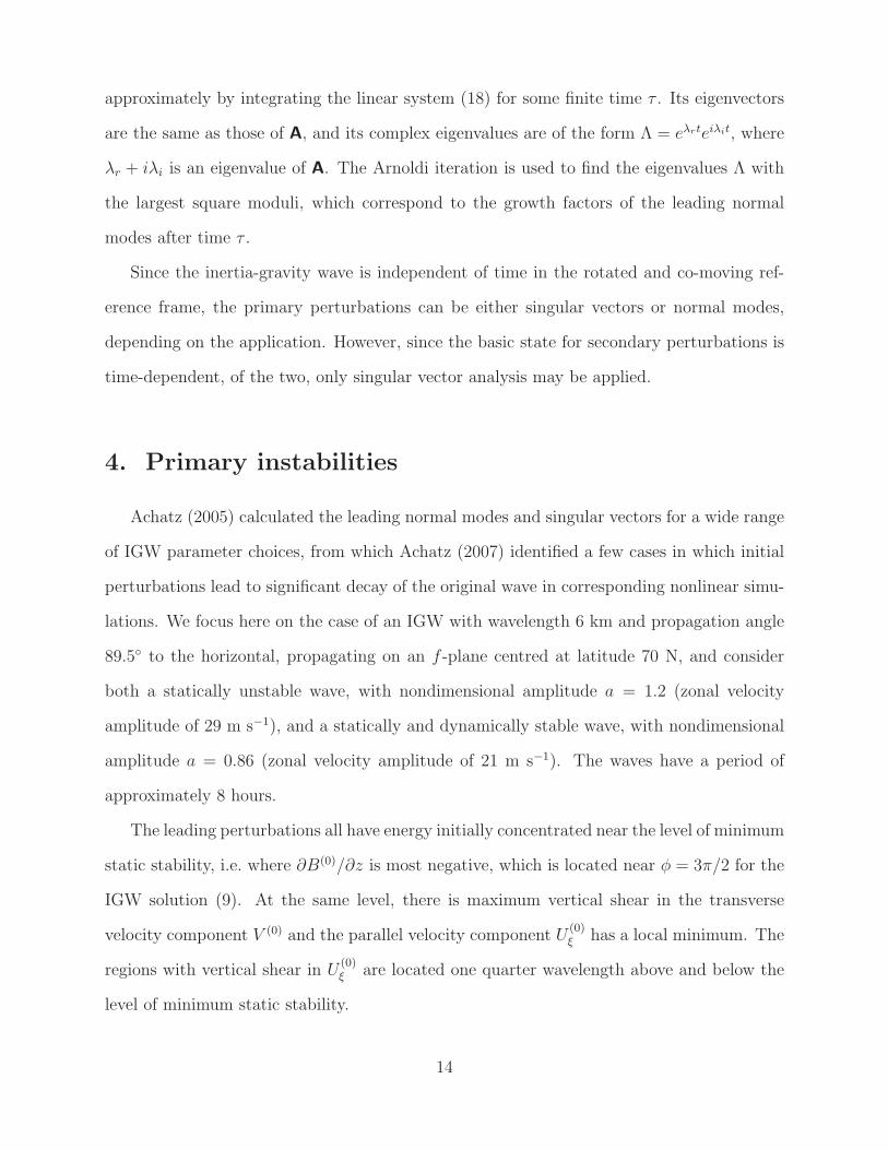
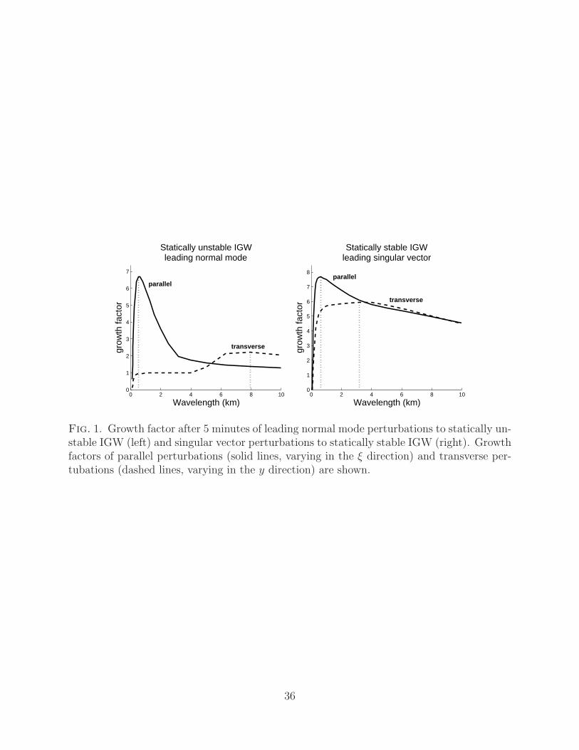
breaking than perturbation by its leading singular vector. The left panel of Fig. 1 shows the
growth factor after 5 minutes as a function of wavelength in the ξ-y plane for the limiting
cases of parallel perturbations (ky = 0), where the perturbation varies in the ξ direction,
and transverse perturbations (kξ = 0), where the perturbation varies in the y direction.
While short wavelength parallel perturbations have the larger growth factors, long wave-
length transverse perturbations lead to more dissipation of the original inertia-gravity wave
(see Fig. 4 of Achatz 2007). An interpretation of this is that the shorter wavelength struc-
tures also have shorter scale in the phase direction, which leads to the formation of strong
gradients, an earlier onset of Kelvin-Helmholtz type instabilities, and relatively rapid non-
linear saturation of the initial instability. Slower developing, larger scale structures (with
correspondingly weaker gradients) that propagate in the phase direction can draw energy
from the shear in all parts of the wave, initially through buoyancy conversion and the gen-
eralized Orr mechanism, and later through the more efficient generalized roll mechanism as
the perturbation propagates away from the level of minimum static stability toward regions
of shear in Uξ.
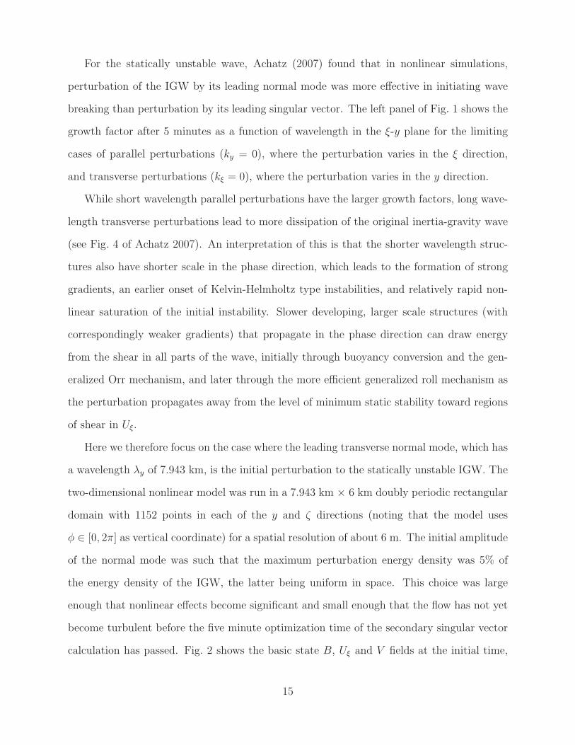
Here we therefore focus on the case where the leading transverse normal mode, which has
a wavelength λy of 7.943 km, is the initial perturbation to the statically unstable IGW. The
two-dimensional nonlinear model was run in a 7.943 km × 6 km doubly periodic rectangular
domain with 1152 points in each of the y and ζ directions (noting that the model uses
φ ∈ [0, 2π] as vertical coordinate) for a spatial resolution of about 6 m. The initial amplitude
of the normal mode was such that the maximum perturbation energy density was 5% of
the energy density of the IGW, the latter being uniform in space. This choice was large
enough that nonlinear effects become significant and small enough that the flow has not yet
become turbulent before the five minute optimization time of the secondary singular vector
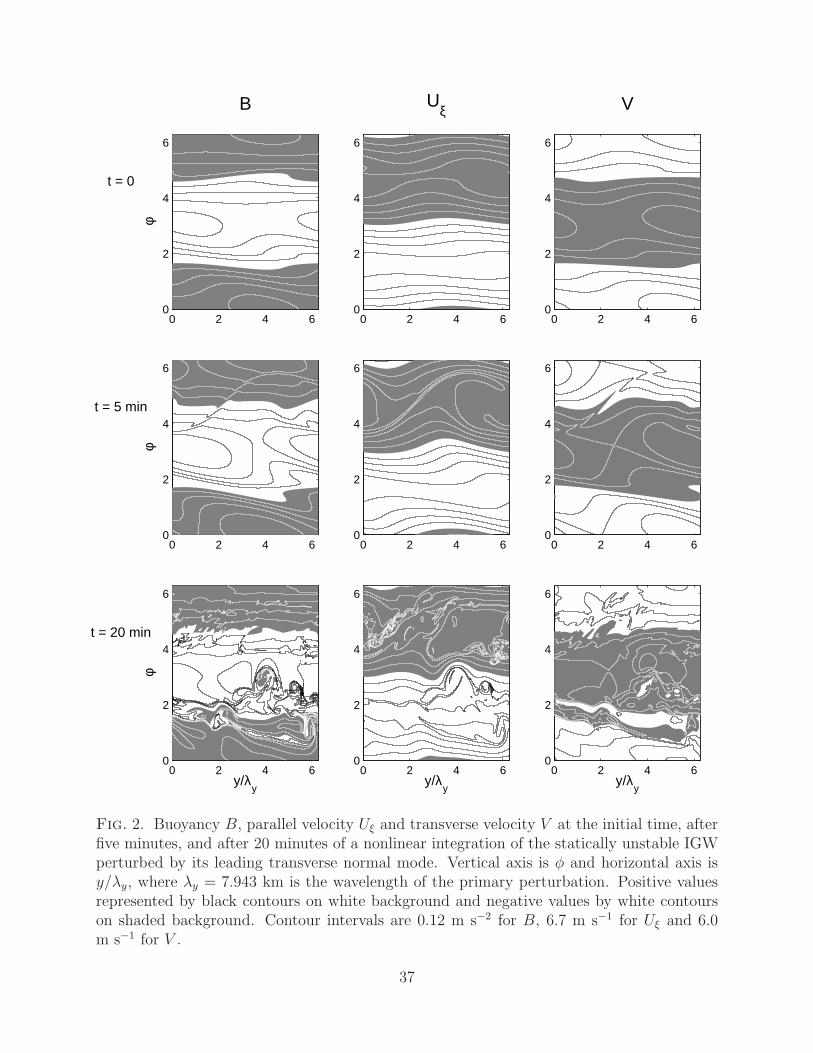
calculation has passed. Fig. 2 shows the basic state B, Uξ and V fields at the initial time,
15
after 5 minutes (the optimization time for the secondary singular vector calculations), and
after 20 minutes.
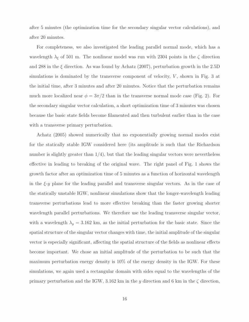
For completeness, we also investigated the leading parallel normal mode, which has a
wavelength λξ of 501 m. The nonlinear model was run with 2304 points in the ζ direction
and 288 in the ξ direction. As was found by Achatz (2007), perturbation growth in the 2.5D
simulations is dominated by the transverse component of velocity, V , shown in Fig. 3 at
the initial time, after 3 minutes and after 20 minutes. Notice that the perturbation remains
much more localized near φ = 3π/2 than in the transverse normal mode case (Fig. 2). For
the secondary singular vector calculation, a short optimization time of 3 minutes was chosen
because the basic state fields become filamented and then turbulent earlier than in the case
with a transverse primary perturbation.
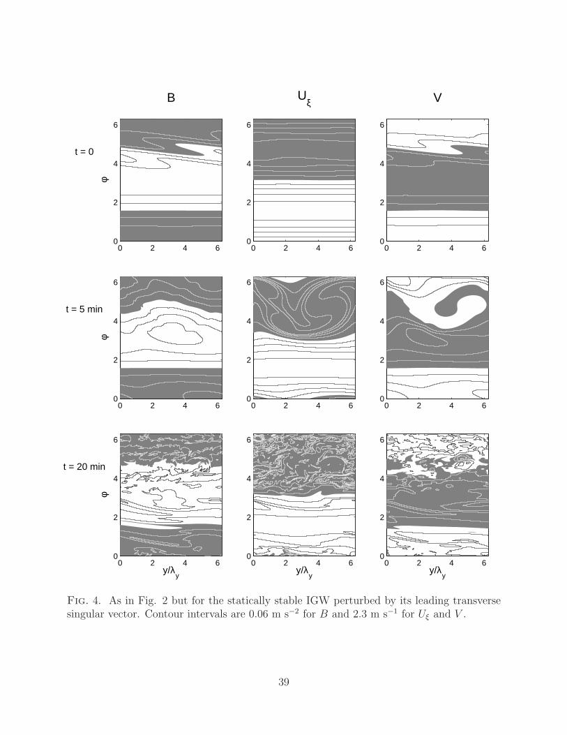
Achatz (2005) showed numerically that no exponentially growing normal modes exist
for the statically stable IGW considered here (its amplitude is such that the Richardson
number is slightly greater than 1/4), but that the leading singular vectors were nevertheless
effective in leading to breaking of the original wave. The right panel of Fig. 1 shows the
growth factor after an optimization time of 5 minutes as a function of horizontal wavelength
in the ξ-y plane for the leading parallel and transverse singular vectors. As in the case of
the statically unstable IGW, nonlinear simulations show that the longer-wavelength leading
transverse perturbations lead to more effective breaking than the faster growing shorter
wavelength parallel perturbations. We therefore use the leading transverse singular vector,
with a wavelength λy = 3.162 km, as the initial perturbation for the basic state. Since the
spatial structure of the singular vector changes with time, the initial amplitude of the singular
vector is especially significant, affecting the spatial structure of the fields as nonlinear effects
become important. We chose an initial amplitude of the perturbation to be such that the
maximum perturbation energy density is 10% of the energy density in the IGW. For these
simulations, we again used a rectangular domain with sides equal to the wavelengths of the
primary perturbation and the IGW, 3.162 km in the y direction and 6 km in the ζ direction,
16
with, respectively, 1152 points and 2304 points for a spatial resolution of approximately 3 m.
Fig. 4 shows the basic state fields at the initial time, after 5 minutes, and after 20 minutes.
5. Secondary instabilities
The secondary instability analysis proceeds as follows: The Boussinesq equations (7) are
linearized about one of the time dependent basic states described above, i.e. the nonlinear
two-dimensional simulations initialized with either a statically unstable IGW perturbed by
its leading parallel or transverse normal mode or a statically stable IGW perturbed by
its leading transverse singular vector. A solution of the form (15) is substituted into the
resulting linearized equations (13), yielding a set of partial differential equations for the
complex amplitudes u′‖, v
′⊥, w
′ζ , and b′ with coefficients periodic in the x‖ and φ directions
and in which the wavelength of the perturbation in the y⊥ direction, λ⊥ = 2π/k⊥, is a
parameter.
The secondary instabilities in which we are interested are of larger scale than the 3 m to
6 m scale resolved by the nonlinear simulations, and the hundreds of integrations necessary
to determine the leading singular vectors at such high resolution would be prohibitively
expensive in terms of computing resources. We found that a grid of 128 × 512 points (a
resolution of 25-50 m in the y direction and the equivalent of 10 m in the φ direction) was
sufficient for the two cases with transverse primary perturbations, the higher resolution in
the φ direction required because the gradients in the basic state are predominantly in the φ
direction. For the statically unstable IGW perturbed by its leading parallel normal mode,
the same 128 × 512 grid was used, representing a more isotropic resolution of 5 to 10 m in
both the ξ and φ directions.
Due to the symmetry of the system, for finite λ⊥, the singular vectors come in pairs with
identical growth factors and spatial structures, corresponding to phase shifts of π/2 in all
variables. We will not distinguish between degenerate singular vectors and by the terms lead-
17
ing, second-leading, and trailing singular vectors, refer to non-degenerate perturbations. The
mode with k⊥ = 0 (i.e. λ⊥ = ∞) is not degenerate, and may be thought of as a modification
of the primary instability due to the nonlinear evolution of the primary perturbation.
We consider the cases of the statically unstable and statically stable IGW separately
in terms of the growth factors and spatial structure of the leading singular vectors and
the dominant energy conversion mechanisms. The singular vectors are then compared to
integrations of the linear model initialized with a random perturbation with |k|−5/3 energy
density spectrum, where k is the perturbation wavevector in the x‖-ζ plane, corresponding
to an isotropic three-dimensional turbulent flow.
a. Statically unstable IGW and transverse primary NM
We begin with the case of the statically unstable IGW perturbed by its leading transverse
normal mode (cf. Fig. 2). For transverse primary perturbations, y⊥ = −ξ and λ⊥ = λξ.
Fig. 5 shows growth factors for the leading singular vectors plotted against λξ. The growth
factor of the leading singular vector is indicated by the solid curve and of the second leading
singular vector by the dashed curve. The single largest growth factor occurs for λξ = 150 m,
but there is a second peak in the growth factor curve of the second leading singular vector
at a wavelength of about 800 m. At each of the two peaks, the 20 leading singular vectors
were computed and their growth factors are indicated by filled diamonds. Shown in the right
panel of the figure are the growth factors of the ensemble of initially random perturbations.
The growth factors of the randomly initialized integrations are naturally much smaller than
those of the singular vectors, the latter being optimally initialized to maximize the growth
factor. One notices again two peaks, one near λξ = 215 m, and the other near λξ = 800 m.
Here, the longer wavelength peak is higher than the shorter wavelength peak. This might be
explained by the fact that for λξ = 800 m, the growth factors of the leading singular vectors
are closer together, while at the λξ = 150 m peak, the growth factor decreases quickly after
the leading singular vector. The random initializations at λξ = 800 m therefore project onto
18
more singular vectors with significant growth factors.
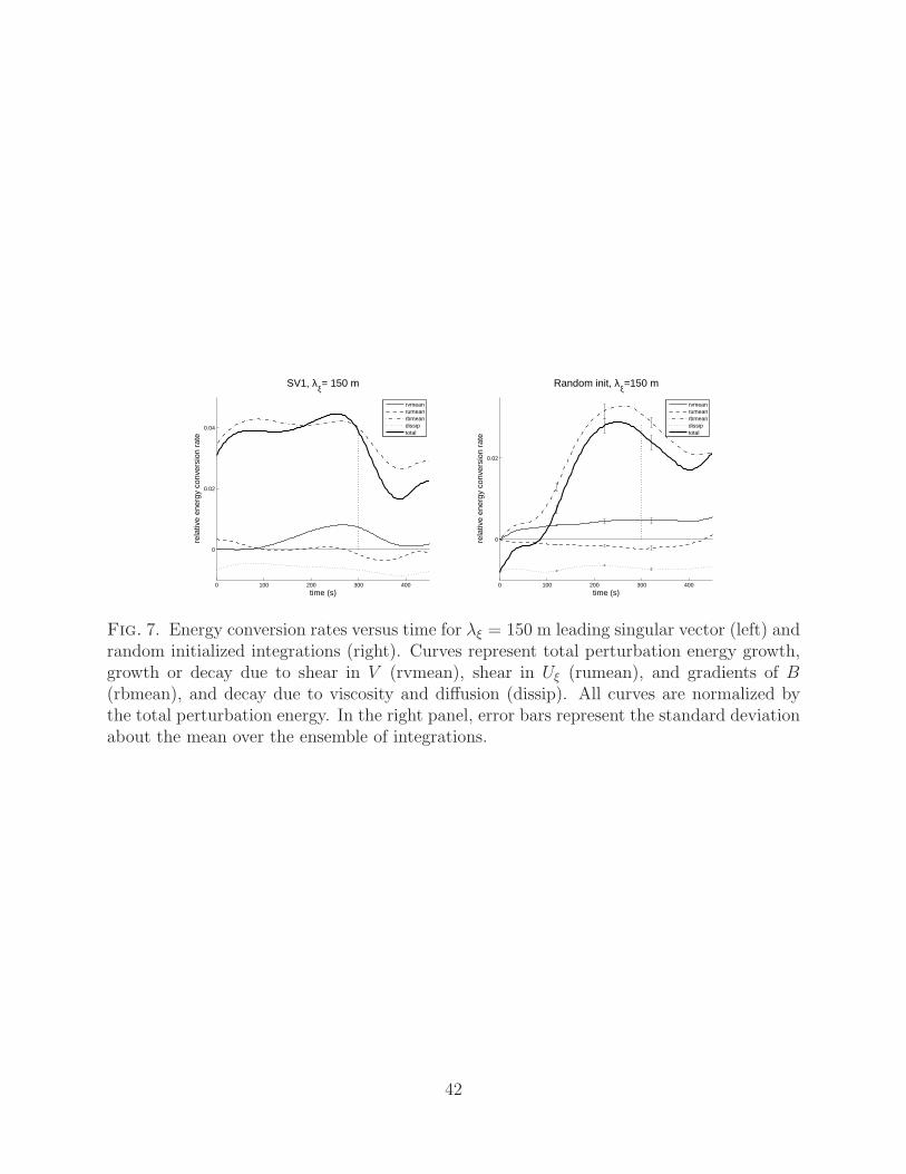
Fig. 6 shows contours of perturbation vertical velocity amplitude w′ζ corresponding to
the leading singular vector at λξ = 150 m plotted over the basic state buoyancy field at the
initial time, halfway to the optimization time, and at the optimization time. Notice how the
time dependent structure of the singular vector follows the location of maximum negative
vertical buoyancy gradient.
For the leading few singular vectors at each of the peaks in the growth factor curve and
for the randomly initialized integrations at the same values of λξ, the integrated energy
conversion rate densities decomposed into contributions from the shears in each velocity
component and from the buoyancy gradient (see Eq. 17) are plotted as functions of time
in Fig. 7. The contributions due to gradients of B represent buoyancy conversion, and the
contributions due to shear in Uξ and V represent growth through the generalized Orr and
roll mechanisms respectively. The linear model is integrated past the optimization time to
see how robust the growth captured by the singular vectors is. All curves are normalized
by the total perturbation energy at each time and can be interpreted as instantaneous
effective growth rates. The energy conversion rates of the leading singular vector match
qualitatively with the corresponding curves for the random initialzations. The dominant
growth mechanism is buoyancy conversion throughout, with a late contribution from the roll
mechanism (growth due to shear in V ). This is consistent with the earlier noted observation
that the energy in the singular vector is concentrated near the location of maximum negative
buoyancy gradient. The randomly initialized integrations take time to become organized but
the energy conversion rate curves match those of the singular vector close to and beyond the
optimization time. The small variation in the conversion curves for the random ensemble,
indicated by error bars, and their resemblance to those of the singular vector suggest that
the dynamics of the singular vectors is representative of the instability of the basic state.
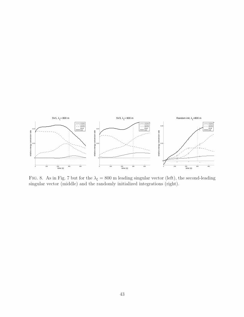
For λξ = 800 m the picture is somewhat different. In this case the second-leading
and trailing singular vectors (not shown for trailing singular vectors) more closely resemble
19
the random ensemble than does the leading singular vector (see Fig. 8). While buoyancy
conversion is the most important mechanism at early times, nearer the optimization time
growth due to shear in Uξ takes over. Contours of perturbation vertical velocity are shown
in Fig. 9 over contours of basic state Uξ at the initial time, at half the optimization time,
and at the optimization time for both the second leading singular vector and for one of the
randomly initialized integrations. The structures in the singular vector perturbation field
are larger scale in y and ζ than their counterparts in the λξ = 150 m case (Fig. 6). This
isotropic scaling (here the scales in all three directions are on the order of 1 km) seems to
be a generic phenomenon: growing perturbations of larger scale in the ξ direction also have
larger scales in the y and ζ directions. Also, the initial concentration of perturbation energy
in the singular vector does not coincide with a region of strong gradient in Uξ, but it does
in the later snapshots. This is consistent with the energy conversion rates plotted in Fig. 8,
where growth due to shear in Uξ becomes important only at later times. The final state of
the randomly initialized integration qualitatively resembles that of the singular vector.
b. Statically unstable IGW and parallel primary NM
For the case of the statically unstable IGW perturbed by its leading parallel normal mode
(cf. Fig. 3), x‖ = ξ and λ⊥ = λy. Fig. 10 shows the growth factors after three minutes of
secondary perturbations as functions of λy for the leading singular vectors and an ensemble
of randomly initialized integrations. There is very close agreement in terms of the position
of the peak and the shape of the growth factor curves, probably because the leading singular
vector is so dominant. The spatial structures of the u′ξ, v
′, and w′ζ components of the leading
singular vector with λy = 270 m are shown in Fig. 11. The perturbations are aligned with
the region of strongest gradient in the basic state V field, again consistent with the energy
conversion rates (Fig. 12), which are dominated by terms proportional to the gradient of V .
Note that while the secondary instabilities of the IGW perturbed by its leading transverse
NM resemble the parallel primary instabilities in terms of length scale and growth mecha-
20
nism, in this case the filamentation that occurs due to the rapid growth of the small-scale
primary perturbation leads to shear instabilities before the large-scale transverse pertur-
bations can grow through the Orr mechanism associated with vertical shear in Uξ. The
small-scale primary and secondary instabilities will, inevitably, saturate rapidly in nonlinear
three-dimensional simulations and are probably not as relevant as the transverse primary
perturbations which lead to more significant dissipation of the original wave.
c. Statically stable IGW and transverse primary SV
The results for the secondary instabilities of the statically stable IGW are somewhat less
clear, but we can still draw conclusions in terms of scales and growth mechanisms like we
did in the case of the statically unstable wave.
Growth factors for the leading secondary singular vectors plotted against λξ for the
statically stable wave are shown in Fig. 13, along with the corresponding growth factor
curves for an ensemble of randomly initialized integrations. There is a single peak near
λξ = 485 m, but the largest growth factors occur for λξ = ∞. The growth factors of the
leading 20 singular vectors at λξ = 485 m are indicated by the filled diamonds, and at
λξ = ∞ by the horizontal line segments at the right edge of the figure. The growth factor
curves for the ensemble of randomly initialized runs do not show a single clear peak, although
individual cases (each curve represents the same initial distribution in y and φ but with a
different value of λξ) have local maxima at λξ < 1 km, and, like the leading singular vector
curve, tend to increase as λξ becomes very large.
The energy conversion rates as functions of time are shown in Fig. 14 for the leading
singular vectors and randomly initialized integrations for both λξ = 485 m and λξ = ∞.
As in the statically unstable IGW case, the linear integrations are extended beyond the
optimization time. While the infinite wavelength runs have larger growth factors at the
optimization time (5 minutes), for a longer run (10 minutes), the short wavelength runs
have much higher growth factors (the growth factors are not shown, but are reflected in the
21
higher conversion rates past the optimization time). For λξ = 485 m, the dominant energy
conversion mechanism is the generalized Orr mechanism (growth due to interaction with
shear in Uξ). For λξ = ∞ both buoyancy conversion and the Orr mechanism are significant.
At later times, and especially beyond the optimization time, the randomly initialized runs
show very similar behaviour to the leading singular vector.
For the λξ = 485 m perturbations, Fig. 15 shows the energy conversion rate densities
due to, respectively, the buoyancy gradient and shear in Uξ and V as functions of space
at the optimization time for both a randomly initialized integration and the same initial
condition projected onto the leading 20 singular vectors. The spatial distribution of the
energy conversion in the full field is largely represented by just the leading singular vectors.
At the optimization time buoyancy conversion is no longer the dominant growth mechanism
for perturbations but is in fact an energy sink. The dominant mechanism at the optimization
time is the generalized Orr mechanism, and as one would expect, it acts in regions of strong
gradients in Uξ (compare with the centre panel of Fig. 4). Note that this result for the
secondary singular vector might be compared with the case of the leading parallel primary
singular vector, whose growth is dominated by buoyancy conversion and the roll mechanism
(Achatz 2005). Evidently the effect of the transverse primary perturbation is to change the
nature of the leading instability with respect to perturbations varying in the ξ (parallel)
direction.
6. Summary and discussion
We have demonstrated a systematic, computationally economical method for investigat-
ing the three dimensionalization of turbulence in breaking inertia gravity waves (IGW) in
the Boussinesq equations. In earlier studies, Achatz (2005; 2007) computed leading linear
instabilities (normal modes and singular vectors) of IGW as functions of perturbation wave-
length and orientation relative to the direction of IGW propagation and used high-resolution
22
“2.5D” simulations to identify the perturbations most important for wave breaking. In the
present study, we have applied singular vector analysis to the equations linearized about
nonlinearly evolving basic states, focusing on two cases identified by Achatz (2007) as lead-
ing to significant dissipation of the IGW in the 2.5D simulations: a statically unstable IGW
perturbed by its leading transverse normal mode, and a statically stable IGW perturbed by
its leading transverse singular vector.
The singular vector results suggest that the dominant spatial scales of the secondary in-
stabilities are an order of magnitude shorter than the scales of the IGW (and of the leading
tranverse primary perturbations). For the statically unstable IGW with wavelength λ = 6
km, perturbed by a transverse normal mode with wavelength λy ≈ 8 km, the leading sec-
ondary singular vector has wavelength of just λξ = 150 m. The singular vector growth factor
spectrum has a second peak near λξ = 800 m, and randomly initialized linear integrations
suggest that the longer wavelength perturbations grow on average somewhat faster than per-
turbations of the shorter scale of the leading singular vector. Two important points to note
are that the scale of the spatial structures of the leading secondary perturbations in the y-ζ
plane is similar to the wavelength of the perturbations in the ξ direction (isotropic scaling)
and that the dominant growth mechanism depends on the spatial scale – buoyancy driven
production of potential energy for the short perturbations and for the longer perturbations,
the generalized Orr mechanism of growth due to shear in the basic state velocity component
Uξ.
For the statically stable IGW perturbed by its leading transverse singular vector of wave-
length λy ≈ 3 km, the secondary perturbations with the largest growth after an optimization
time of 5 minutes have infinite λξ (i.e. they do not vary in the ξ direction), but longer in-
tegrations of the linear model show that perturbations with λξ = 485 m grow significantly
more.
We also consider the statically unstable IGW perturbed its leading parallel normal mode,
which has the largest linear growth rate of any perturbation but appears to saturate quickly
23
in 2.5D simulations without leading to strong dissipation of the original wave. Like the
primary perturbations, the leading secondary singular vectors in this case grow through a
shear instability associated with basic state V .
A weakness of singular vector analysis as a diagnostic tool is that the spatial structures it
identifies are time-dependent, so they cannot be expected to be recognized in observations.
To address this point, we compared the growth factor spectra, spatial scales and growth
mechanisms of the singular vectors with randomly initialized integrations of the linear model
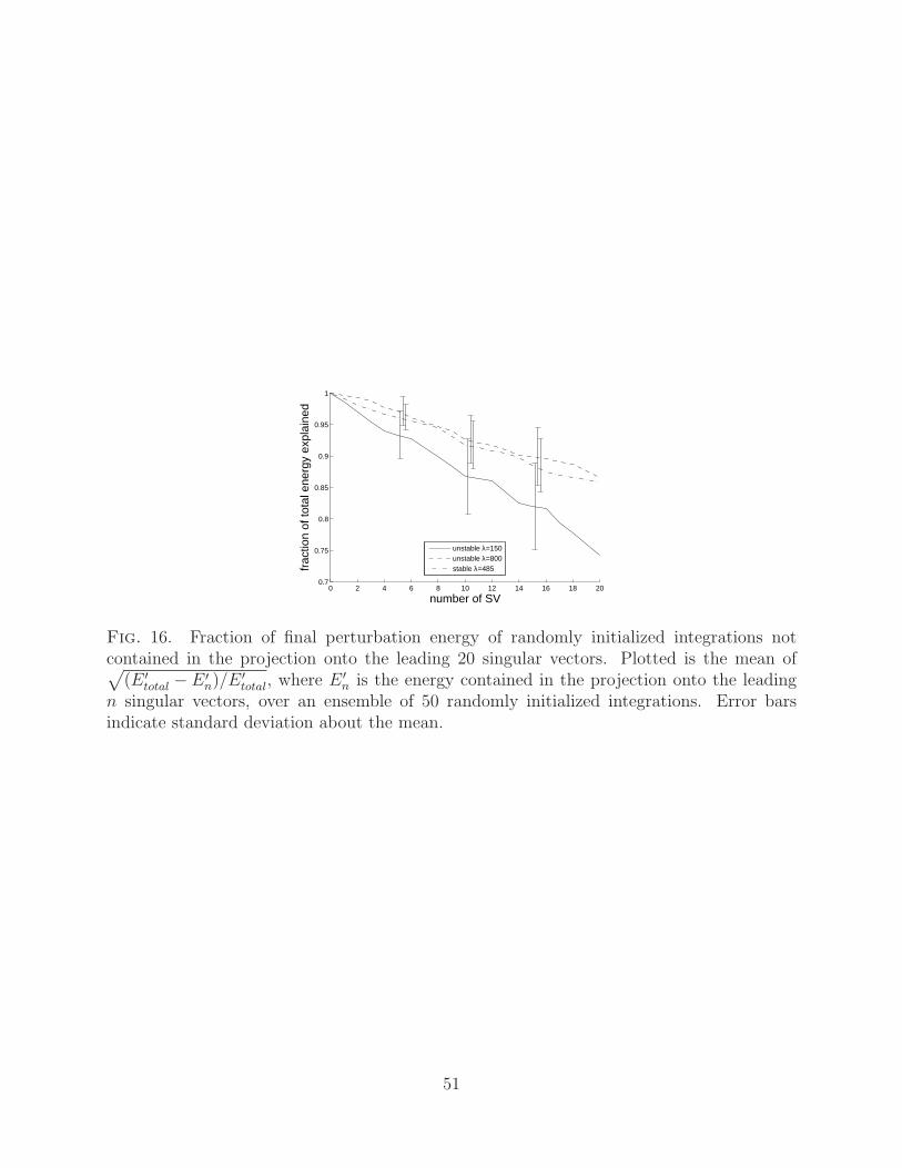
and found consistent agreement. A natural question is how much of the growth of random
perturbations can be “explained” by the leading singular vectors. Since singular vectors
are mutually orthogonal at both the initial and optimization times, it is a simple matter
to project the state at the optimization time of the randomly initialized integrations onto a
subset of the singular vectors. The energy not contained in the leading n singular vectors
for λξ = 150 m and λξ = 800 m for the statically unstable IGW perturbed by its leading
transverse NM and λξ = 485 m for the statically stable IGW is plotted against n in Fig. 16.
Between about 10% and 30% of the total perturbation energy is contained in the leading 20
singular vectors. This is considerable since the discretized system has on the order of 104
degrees of freedom.
Since wave-breaking is an inherently three dimensional and multi-scale phenomenon,
definitive conclusions require three-dimensional nonlinear simulations with high enough reso-
lution to resolve the small scales of turbulence and domains large enough to contain the large-
scale instabilities which dominate the early phase of wave breaking. While high-resolution
three-dimensional numerical simulations of breaking high frequency gravity waves have been
done (Fritts et al. 2009a,b), to our knowledge no such simulations of breaking low-frequency
inertia-gravity waves (waves affected by rotation) have yet been done. Our results suggest
that the scales of the instabilities are such that the dominant structures can be contained
in a domain considerably smaller than the cube of the wavelength of the IGW, and the
rotated coordinate system allows for the accommodation of the very large horizontal scale
24
of IGW in the earth frame. Such simulations, initialized with the IGW, a leading primary
perturbation, and a leading secondary singular vector, would serve as data for evaluating
large eddy simulation (LES) methods as well as gravity-wave drag parameterization schemes
used in climate and general circulation models.
Acknowledgments.
This work was supported by the Deutsche Forschungsgemeinschaft through the Met-
Strom Priority Research Program (SPP 1276) and the grant Ac 71/4-1 and by the Leibniz-
Gemeinschaft (WGL) through the PAKT program.
25
REFERENCES
Achatz, U., 2005: On the role of optimal perturbations in the instability of monochromatic
gravity waves. Phys. Fluids, 17, 1–27.
Achatz, U., 2007: The primary nonlinear dynamics of modal and nonmodal perturbations
of monochromatic inertia-gravity waves. J. Atmos. Sci., 64, 74–95.
Achatz, U. and G. Schmitz, 2006: Shear and static instability of inertia-gravity wave packets:
Short-term modal and nonmodal growth. J. Atmos. Sci., 63, 397–413.
Andreassen, O., C. E. Wasberg, D. C. Fritts, and J. R. Isler, 1994: Gravity wave breaking
in two and three dimensions 1. Model description and comparison of two-dimensional
evolutions. J. Geophys. Res., 99, 8095–8108.
Bakas, N. A., P. J. Ioannou, and G. E. Kefaliakos, 2001: The emergence of coherent struc-
tures in stratified shear flow. J. Atmos. Sci, 58, 2790–2806.
Bretherton, F. P., 1966: The propagation of groups of internal gravity waves in a shear flow.
Quart. J. Roy. Met. Soc., 92, 466–480.
Drazin, P. G., 1977: On the instability of an internal gravity wave. Proc. R. Soc. London,
356, 411–432.
Dunkerton, T. J., 1997: Shear instability of internal inertia-gravity waves. J. Atmos. Sci.,
54, 1628–1641.
Durran, D. R., 1999: Numerical Methods for Wave Equations in Geophysical Fluid Dynam-
ics. Springer, New York, 465pp. pp.
26
Farrell, B. F. and P. J. Ioannou, 1996a: Generalized stability theory. Part I: Autonomous
operators. J. Atmos. Sci., 53, 2025–2040.
Farrell, B. F. and P. J. Ioannou, 1996b: Generalized stability theory. Part II: Nonautonomous
operators. J. Atmos. Sci., 53, 2041–2053.
Fritts, D. C. and M. J. Alexander, 2003: Gravity wave dynamics and effects in the middle
atmosphere. Rev. Geophys., 41, 3.1–3.64.
Fritts, D. C., J. R. Isler, and O. Andreassen, 1994: Gravity wave breaking in two and three
dimensions 2. Three-dimensional evolution and instability structure. J. Geophys. Res., 99,
8109–8123.
Fritts, D. C., S. L. Vadas, and J. A. Werne, 2006: Mean and variable forcing of the middle
atmosphere by gravity waves. J. Atmos. Sol.-Terr. Phys., 68, 247–265.
Fritts, D. C., L. Wang, J. Werne, T. Lund, and K. Wan, 2009a: Gravity wave instability
dynamics at high Reynolds numbers. Part I: Wave field evolution at large amplitudes and
high frequencies. J. Atmos. Sci., 66, 1126–1148.
Fritts, D. C., L. Wang, J. Werne, T. Lund, and K. Wan, 2009b: Gravity wave instabil-
ity dynamics at high Reynolds numbers. Part II: Turbulence evolution, structure, and
anisotropy. J. Atmos. Sci., 66, 1149–1171.
Giering, R. and T. Kaminski, 1998: Recipes for adjoint code construction. ACM Trans.
Math. Software, 24, 437–474.
Grimshaw, R., 1975: Internal gravity waves: critical layer absorption in a rotating fluid. J.
Fluid Mech., 70, 287–304.
Holton, J. R., 1982: The role of gravity wave induced drag and diffusion in the momentum
budget of the mesosphere. J. Atmos. Sci., 39, 791–799.
27
Houghton, J. T., 1978: The stratosphere and the mesosphere. Quart. J. Roy. Meteor. Soc.,
104, 1–29.
Howard, L. N., 1961: Note on a paper of John W. Miles. J. Fluid Mech., 10, 509–512.
Klaassen, G. P. and W. R. Peltier, 1985a: Evolution of finite amplitude Kelvin-Helmholtz
billows in two spatial dimensions. J. Atmos. Sci., 42, 1321–1339.
Klaassen, G. P. and W. R. Peltier, 1985b: The onset of turbulence in finite-amplitude
Kelvin-Helmholtz billows. J. Fluid Mech., 155, 1–35.
Klostermeyer, J., 1983: On parametric instabilities of finite-amplitude internal gravity waves.
J. Fluid Mech., 119, 367–377.
Lehoucq, R. B., D. C. Sorensen, and C. Yang, 1998: ARPACK Users’ Guide: Solution of
large-scale eigenvalue problems with implicitly restarted Arnoldi methods. SIAM, 160 pp.
Lelong, M.-P. and T. J. Dunkerton, 1998a: Inertia-gravity wave breaking in three dimensions.
Part I: Convectively stable waves. J. Atmos. Sci., 55, 2473–2488.
Lelong, M.-P. and T. J. Dunkerton, 1998b: Inertia-gravity wave breaking in three dimensions.
Part II: Convectively unstable waves. J. Atmos. Sci., 55, 2489–2501.
Lindzen, R. S., 1981: Turbulence and stress owing to gravity wave and tidal breakdown. J.
Geophys. Res., 86, 9707–9714.
Lindzen, R. S. and J. R. Holton, 1968: A theory of the quasi-biennial oscillation. J. Atmos.
Sci., 25, 1095–1107.
McLandress, C., 1998: On the importance of gravity waves in the middle atmosphere and
their parameterization in general circulation models. J. Atmos. Sol.-Terr. Phy., 60, 1357–
1383.
28
Mied, R. P., 1976: The occurrence of parametric instabilities in finite amplitude internal
gravity waves. J. Fluid Mech., 78, 763–784.
Miles, J. W., 1961: On the stability of heterogeneous shear flows. J. Fluid Mech., 10, 496–
508.
Muller, P., 1976: On the diffusion of momentum and mass by internal gravity waves. J. Fluid
Mech., 77, 789–823.
Nicolls, M. J., R. H. Varney, S. L. Vadas, P. A. Stamus, C. J. Heinselman, R. B. Cosgrove,
and M. C. Kelley, 2010: Influence of an inertia-gravity wave on mesospheric dynamics: A
case study with the Poker Flat Incoherent Scatter Radar. J. Geophys. Res., 115, D00N02,
doi:10.1029/2010JD014042.
Yau, K. H., G. P. Klaassen, and L. J. Sonmor, 2004: Principal instabilities of large amplitude
inertio-gravity waves. Phys. Fluids, 16, 936–951.
29
List of Tables
1 Summary of model parameters. 31
30
Statically Unstable IGW Statically Stable IGW
IGW amplitude withrespect to static instability
a = 1.2(u = 29 m s−1)
a = 0.86(u = 21 m s−1)
IGW wavelength, period 6 km, 8 h 6 km, 8 h
Primary perturbation
trans. NM: λy = 7.943 km
para. NM: λξ = 501 m
ampl. Emaxpert/EIGW = 5%
trans. SV: λy = 3.162 km
ampl. Emaxpert/EIGW = 10%
Resolution of nonlinear2.5D simulation (nx‖ × nφ)
trans. NM: 1152 × 1152
para. NM: 288 × 2304trans. SV: 1152 × 2304
Resolution for secondarysingular vector calculation(nx‖ × nφ)
128 × 512 128 × 512
Wavelengths of leadingsecondary perturbations
trans. NM: λξ = 150 m, 800 m
para. NM: λy = 270 mλξ = 485 m, ∞
Table 1. Summary of model parameters.
31
List of Figures
1 Growth factor after 5 minutes of leading normal mode perturbations to stati-
cally unstable IGW (left) and singular vector perturbations to statically stable
IGW (right). Growth factors of parallel perturbations (solid lines, varying in
the ξ direction) and transverse pertubations (dashed lines, varying in the y
direction) are shown. 36
2 Buoyancy B, parallel velocity Uξ and transverse velocity V at the initial time,
after five minutes, and after 20 minutes of a nonlinear integration of the stati-
cally unstable IGW perturbed by its leading transverse normal mode. Vertical
axis is φ and horizontal axis is y/λy, where λy = 7.943 km is the wavelength
of the primary perturbation. Positive values represented by black contours
on white background and negative values by white contours on shaded back-
ground. Contour intervals are 0.12 m s−2 for B, 6.7 m s−1 for Uξ and 6.0
m s−1 for V . 37
3 Transverse velocity V as a function of ξ and φ at the initial time, after three
minutes, and after 20 minutes of a nonlinear integration of the statically un-
stable IGW perturbed by its leading parallel normal mode, which has wave-
length λξ = 501 m. Positive values represented by black contours on white
background and negative values by white contours on shaded background.
Contour intervals are 3.6 m s−1. 38
4 As in Fig. 2 but for the statically stable IGW perturbed by its leading trans-
verse singular vector. Contour intervals are 0.06 m s−2 for B and 2.3 m s−1
for Uξ and V . 39
32
5 Left: Growth factor of leading secondary singular vectors versus wavelength in
the ξ direction for the basic state consisting of the statically unstable inertia-
gravity wave perturbed by its leading transverse normal mode. Filled dia-
monds represent the leading 20 singular vectors at λξ = 150 m and λξ = 800
m. Right: Growth factors for an ensemble of randomly initialized integrations
with heavy dashed line representing the ensemble mean. 40
6 Contours of perturbation vertical velocity amplitude w′ζ for the leading sec-
ondary singular vector (with λξ = 150 m) of the perturbed statically unstable
IGW over the basic state buoyancy field (shading, cf. upper- and middle-left
panels of Fig. 2) at the initial time, half way to the optimization time and at
the optimization time. Initially concentrated near maximum negative buoy-
ancy gradient, the perturbation migrates in space with time due to advection
by the basic state V and Wζ fields. Contours of w′ζ are in increments of 20%
of the maximum value at the corresponding time (amplitudes are increasing
roughly exponentially with time). Black (white) contours represent positive
(negative) values. 41
7 Energy conversion rates versus time for λξ = 150 m leading singular vector
(left) and random initialized integrations (right). Curves represent total per-
turbation energy growth, growth or decay due to shear in V (rvmean), shear
in Uξ (rumean), and gradients of B (rbmean), and decay due to viscosity and
diffusion (dissip). All curves are normalized by the total perturbation energy.
In the right panel, error bars represent the standard deviation about the mean
over the ensemble of integrations. 42
8 As in Fig. 7 but for the λξ = 800 m leading singular vector (left), the second-
leading singular vector (middle) and the randomly initialized integrations
(right). 43
33
9 Contours of perturbation vertical velocity amplitude w′ζ for secondary pertur-
bations with λξ = 800 m to the statically unstable IGW over the basic state
parallel velocity field Uξ (shading, cf. upper and middle centre panels in Fig.
2) at the initial time, half way to the optimization time and at the optimiza-
tion time. Top row: second leading singular vector. Bottom row: randomly
initialized integrations. Contours of w′ζ are as in Fig. 6. 44
10 Growth factor of leading secondary singular vectors (left) and randomly ini-
tialized integrations (right) versus wavelength in the y direction for the IGW
perturbed by its leading parallel normal mode. 45
11 Contours of perturbation velocity amplitude u′ξ, v
′, and w′ζ , over basic state
transverse velocity field V (shading) for secondary perturbations with λy =
270 m to the statically unstable IGW perturbed by its leading parallel normal
mode at initial time (top row) and optimization time (bottom row). Contours
are normalized by perturbation total energy as in Fig. 6. 46
12 As in Fig. 7 but for the IGW perturbed by its leading parallel normal mode:
leading singular vector (left) and randomly initialized integrations (right) with
λy = 270 m. 47
13 As in Fig. 5 but for the perturbed statically stable IGW. Horizontal lines at
right edge of left panel represent growth factors for λξ = ∞. 48
14 As in Fig. 7 but for λξ = 485 m (top row) and λξ = ∞ (bottom row) and
statically stable IGW. 49
34
15 Statically stable IGW case. Energy conversion rate density involving gradients
of B (left), shear in Uξ (centre), and shear in V (right) at the optimization time
for a randomly initialized integration (bottom) and the same initial condition
projected onto the leading singular vectors (top). Shading is scaled so as to
show the sign (light positive, dark negative) and spatial distribution of each
energy conversion mechanism but not the relative magnitudes of the three
contributions. 50
16 Fraction of final perturbation energy of randomly initialized integrations not
contained in the projection onto the leading 20 singular vectors. Plotted is
the mean of√
(E ′total − E ′
n)/E′total, where E ′
n is the energy contained in the
projection onto the leading n singular vectors, over an ensemble of 50 ran-
domly initialized integrations. Error bars indicate standard deviation about
the mean. 51
35
0 2 4 6 8 100
1
2
3
4
5
6
7
Wavelength (km)
grow
th fa
ctor
Statically unstable IGWleading normal mode
0 2 4 6 8 100
1
2
3
4
5
6
7
8
Wavelength (km)
grow
th fa
ctor
Statically stable IGWleading singular vector
parallel
transverse
parallel
transverse
Fig. 1. Growth factor after 5 minutes of leading normal mode perturbations to statically un-stable IGW (left) and singular vector perturbations to statically stable IGW (right). Growthfactors of parallel perturbations (solid lines, varying in the ξ direction) and transverse per-tubations (dashed lines, varying in the y direction) are shown.
36
0 2 4 60
2
4
6φ
0 2 4 60
2
4
6
φ
0 2 4 60
2
4
6
φ
y/λy
0 2 4 60
2
4
6
0 2 4 60
2
4
6
0 2 4 60
2
4
6
y/λy
0 2 4 60
2
4
6
0 2 4 60
2
4
6
0 2 4 60
2
4
6
y/λy
B Uξ V
t = 0
t = 5 min
t = 20 min
Fig. 2. Buoyancy B, parallel velocity Uξ and transverse velocity V at the initial time, afterfive minutes, and after 20 minutes of a nonlinear integration of the statically unstable IGWperturbed by its leading transverse normal mode. Vertical axis is φ and horizontal axis isy/λy, where λy = 7.943 km is the wavelength of the primary perturbation. Positive valuesrepresented by black contours on white background and negative values by white contourson shaded background. Contour intervals are 0.12 m s−2 for B, 6.7 m s−1 for Uξ and 6.0m s−1 for V .
37
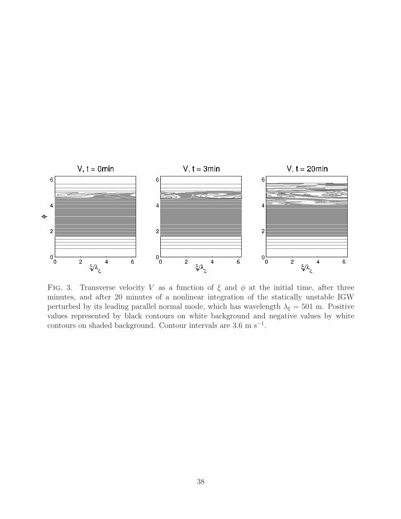
Fig. 3. Transverse velocity V as a function of ξ and φ at the initial time, after threeminutes, and after 20 minutes of a nonlinear integration of the statically unstable IGWperturbed by its leading parallel normal mode, which has wavelength λξ = 501 m. Positivevalues represented by black contours on white background and negative values by whitecontours on shaded background. Contour intervals are 3.6 m s−1.
38
0 2 4 60
2
4
6
φ
0 2 4 60
2
4
6
φ
0 2 4 60
2
4
6
φ
y/λy
0 2 4 60
2
4
6
0 2 4 60
2
4
6
0 2 4 60
2
4
6
y/λy
0 2 4 60
2
4
6
0 2 4 60
2
4
6
0 2 4 60
2
4
6
y/λy
B Uξ V
t = 0
t = 5 min
t = 20 min
Fig. 4. As in Fig. 2 but for the statically stable IGW perturbed by its leading transversesingular vector. Contour intervals are 0.06 m s−2 for B and 2.3 m s−1 for Uξ and V .
39
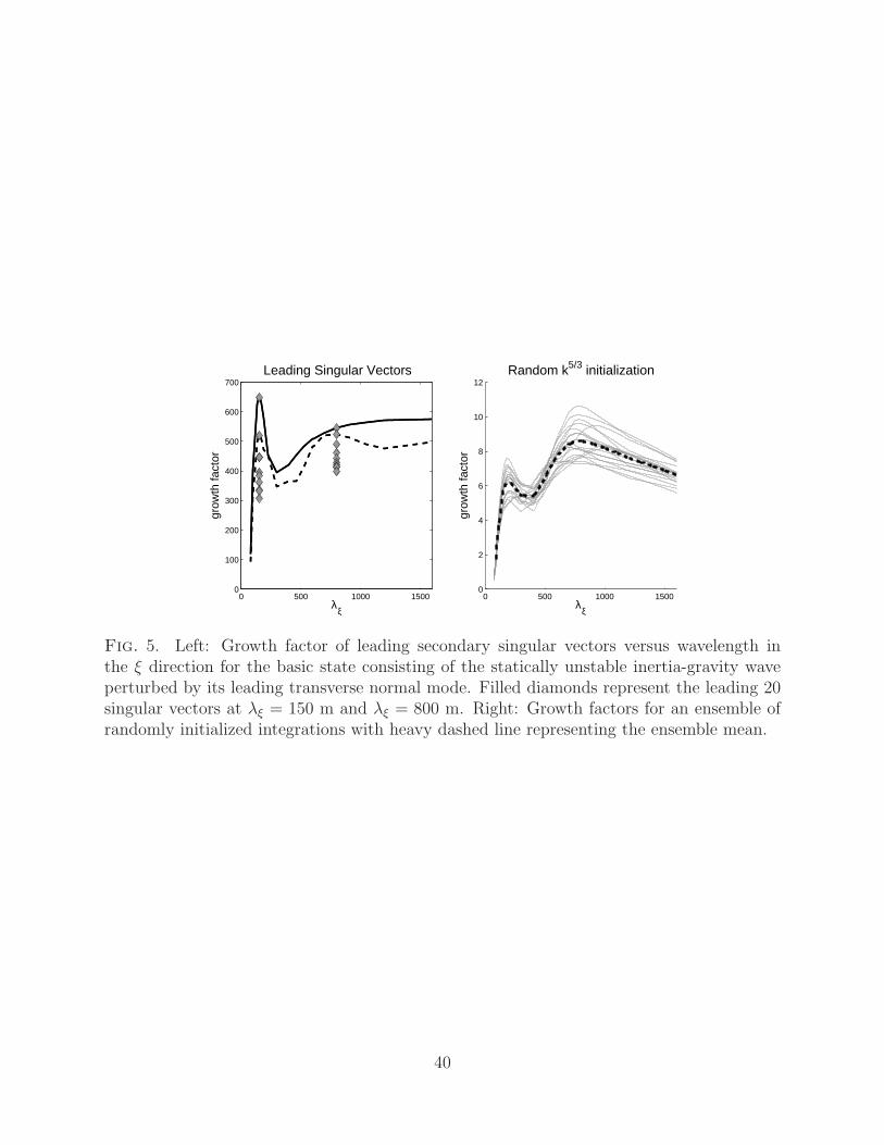
0 500 1000 15000
100
200
300
400
500
600
700Leading Singular Vectors
λξ
grow
th fa
ctor
0 500 1000 15000
2
4
6
8
10
12Random k5/3 initialization
λξ
grow
th fa
ctor
Fig. 5. Left: Growth factor of leading secondary singular vectors versus wavelength inthe ξ direction for the basic state consisting of the statically unstable inertia-gravity waveperturbed by its leading transverse normal mode. Filled diamonds represent the leading 20singular vectors at λξ = 150 m and λξ = 800 m. Right: Growth factors for an ensemble ofrandomly initialized integrations with heavy dashed line representing the ensemble mean.
40
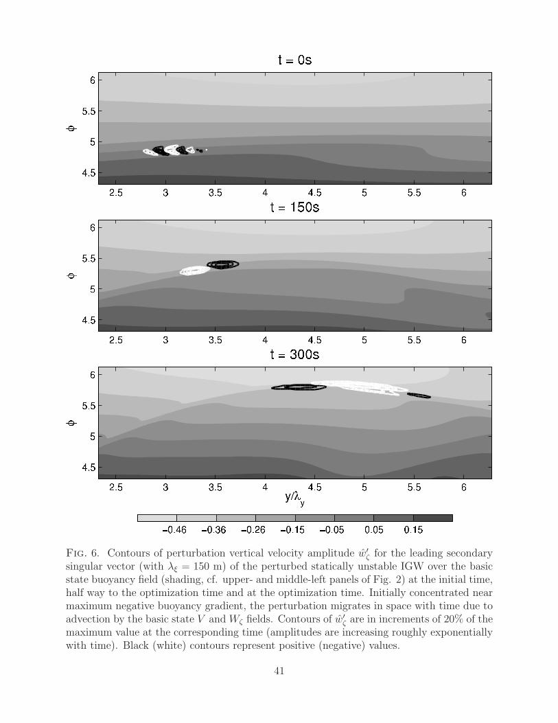
Fig. 6. Contours of perturbation vertical velocity amplitude w′ζ for the leading secondary
singular vector (with λξ = 150 m) of the perturbed statically unstable IGW over the basicstate buoyancy field (shading, cf. upper- and middle-left panels of Fig. 2) at the initial time,half way to the optimization time and at the optimization time. Initially concentrated nearmaximum negative buoyancy gradient, the perturbation migrates in space with time due toadvection by the basic state V and Wζ fields. Contours of w
′ζ are in increments of 20% of the
maximum value at the corresponding time (amplitudes are increasing roughly exponentiallywith time). Black (white) contours represent positive (negative) values.
41
0 100 200 300 400
0
0.02
0.04
time (s)
rela
tive
ener
gy c
onve
rsio
n ra
te
SV1, λξ= 150 m
rvmeanrumeanrbmeandissiptotal
0 100 200 300 400
0
0.02
time (s)
rela
tive
ener
gy c
onve
rsio
n ra
te
Random init, λξ=150 m
rvmeanrumeanrbmeandissiptotal
Fig. 7. Energy conversion rates versus time for λξ = 150 m leading singular vector (left) andrandom initialized integrations (right). Curves represent total perturbation energy growth,growth or decay due to shear in V (rvmean), shear in Uξ (rumean), and gradients of B(rbmean), and decay due to viscosity and diffusion (dissip). All curves are normalized bythe total perturbation energy. In the right panel, error bars represent the standard deviationabout the mean over the ensemble of integrations.
42
0 100 200 300 400
0
0.02
0.04
time (s)
rela
tive
ener
gy c
onve
rsio
n ra
te
SV1, λξ= 800 m
rvmeanrumeanrbmeandissiptotal
0 100 200 300 400
0
0.02
0.04
time (s)
rela
tive
ener
gy c
onve
rsio
n ra
te
SV3, λξ= 800 m
rvmeanrumeanrbmeandissiptotal
0 100 200 300 400
0
0.02
0.04
time (s)
rela
tive
ener
gy c
onve
rsio
n ra
te
Random init, λξ=800 m
rvmeanrumeanrbmeandissiptotal
Fig. 8. As in Fig. 7 but for the λξ = 800 m leading singular vector (left), the second-leadingsingular vector (middle) and the randomly initialized integrations (right).
43
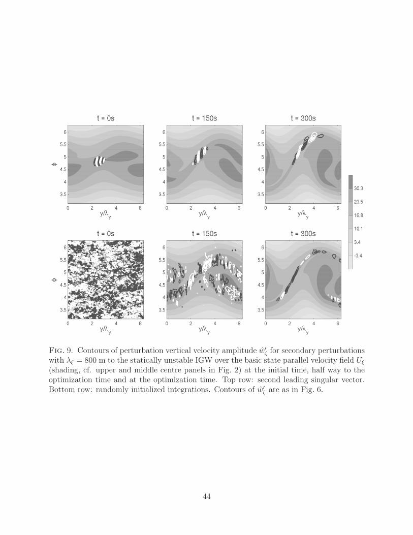
Fig. 9. Contours of perturbation vertical velocity amplitude w′ζ for secondary perturbations
with λξ = 800 m to the statically unstable IGW over the basic state parallel velocity field Uξ
(shading, cf. upper and middle centre panels in Fig. 2) at the initial time, half way to theoptimization time and at the optimization time. Top row: second leading singular vector.Bottom row: randomly initialized integrations. Contours of w′
ζ are as in Fig. 6.
44
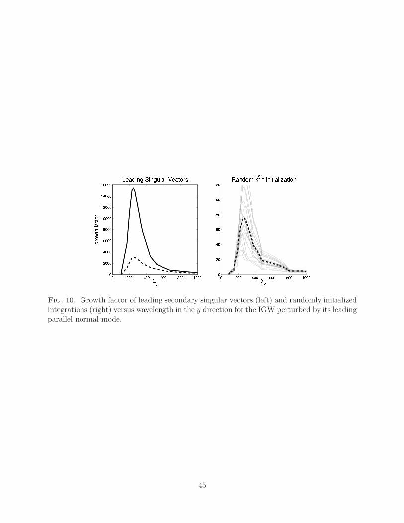
Fig. 10. Growth factor of leading secondary singular vectors (left) and randomly initializedintegrations (right) versus wavelength in the y direction for the IGW perturbed by its leadingparallel normal mode.
45
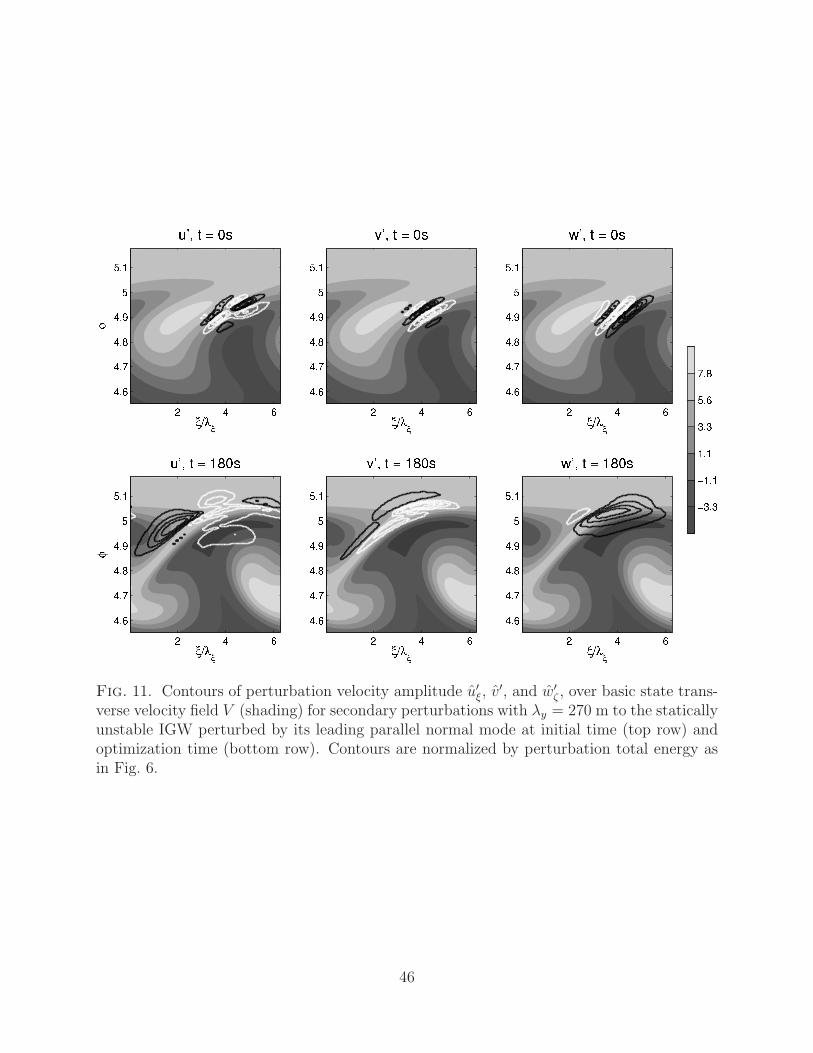
Fig. 11. Contours of perturbation velocity amplitude u′ξ, v
′, and w′ζ , over basic state trans-
verse velocity field V (shading) for secondary perturbations with λy = 270 m to the staticallyunstable IGW perturbed by its leading parallel normal mode at initial time (top row) andoptimization time (bottom row). Contours are normalized by perturbation total energy asin Fig. 6.
46
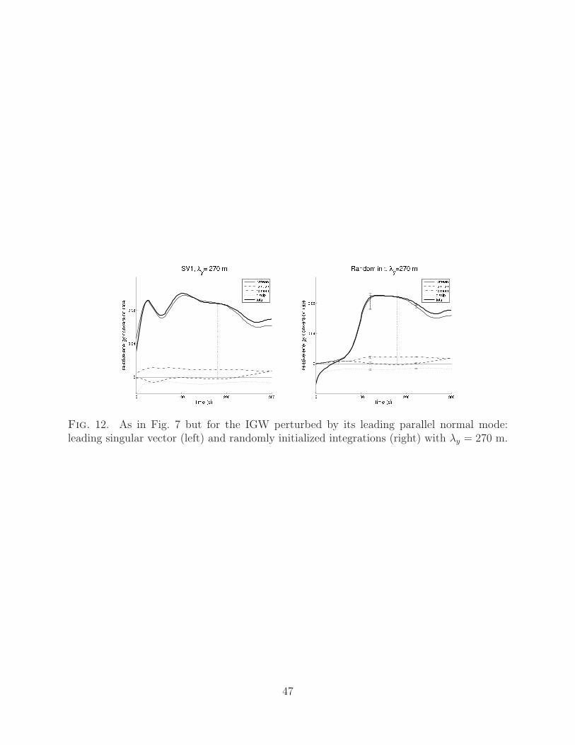
Fig. 12. As in Fig. 7 but for the IGW perturbed by its leading parallel normal mode:leading singular vector (left) and randomly initialized integrations (right) with λy = 270 m.
47
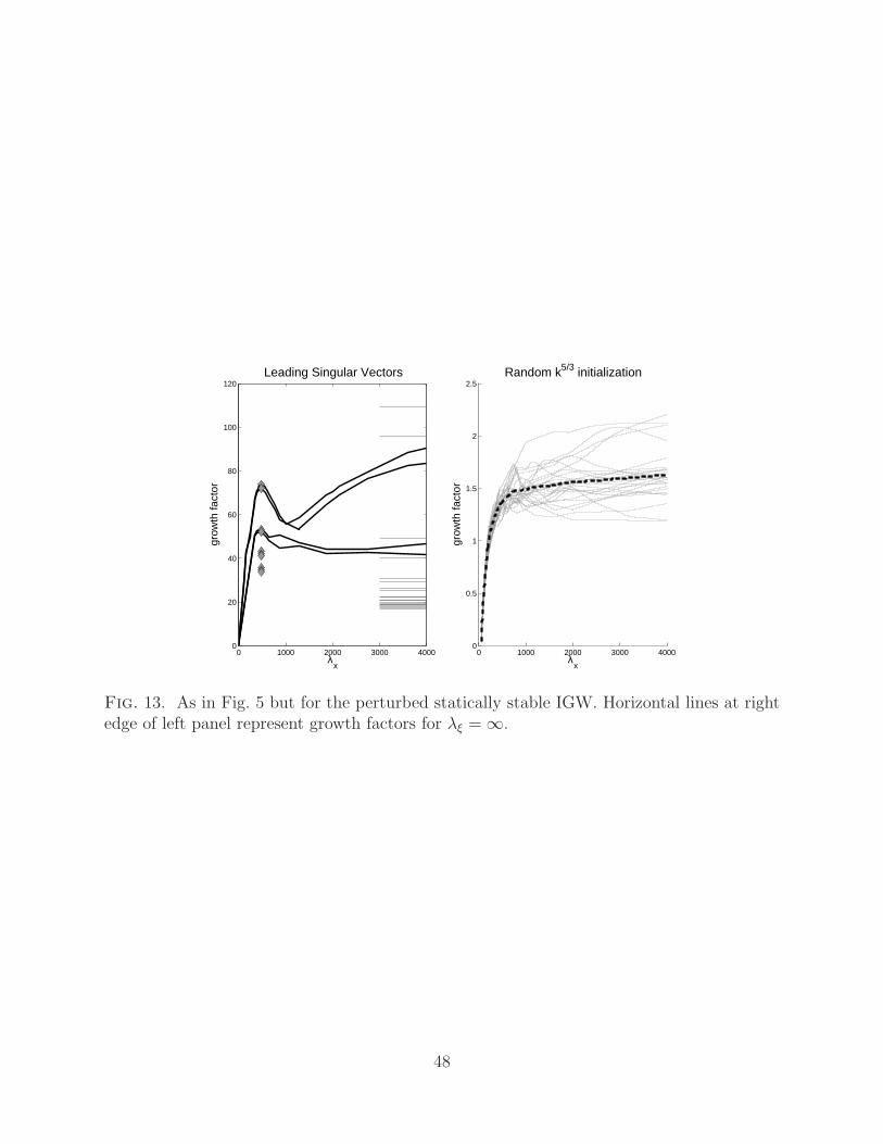
0 1000 2000 3000 40000
20
40
60
80
100
120Leading Singular Vectors
λx
grow
th fa
ctor
0 1000 2000 3000 40000
0.5
1
1.5
2
2.5Random k5/3 initialization
λx
grow
th fa
ctor
Fig. 13. As in Fig. 5 but for the perturbed statically stable IGW. Horizontal lines at rightedge of left panel represent growth factors for λξ = ∞.
48
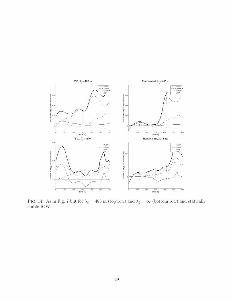
0 100 200 300 400 500 600
0
0.02
0.04
0.06
time (s)
rela
tive
ener
gy c
onve
rsio
n ra
te
SV1, λξ= 485 m
rvmeanrumeanrbmeandissiptotal
0 100 200 300 400 500 600
0
0.02
0.04
0.06
time (s)
rela
tive
ener
gy c
onve
rsio
n ra
te
Random init, λξ= 485 m
rvmeanrumeanrbmeandissiptotal
0 100 200 300 400 500 600
0
0.02
0.04
time (s)
rela
tive
ener
gy c
onve
rsio
n ra
te
SV1, λξ= infty
rvmeanrumeanrbmeandissiptotal
0 100 200 300 400 500 600
0
0.02
time (s)
rela
tive
ener
gy c
onve
rsio
n ra
te
Random init, λξ= infty
rvmeanrumeanrbmeandissiptotal
Fig. 14. As in Fig. 7 but for λξ = 485 m (top row) and λξ = ∞ (bottom row) and staticallystable IGW.
49
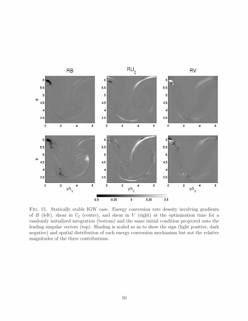
Fig. 15. Statically stable IGW case. Energy conversion rate density involving gradientsof B (left), shear in Uξ (centre), and shear in V (right) at the optimization time for arandomly initialized integration (bottom) and the same initial condition projected onto theleading singular vectors (top). Shading is scaled so as to show the sign (light positive, darknegative) and spatial distribution of each energy conversion mechanism but not the relativemagnitudes of the three contributions.
50
0 2 4 6 8 10 12 14 16 18 200.7
0.75
0.8
0.85
0.9
0.95
1
number of SV
frac
tion
of to
tal e
nerg
y ex
plai
ned
unstable λ=150unstable λ=800stable λ=485
Fig. 16. Fraction of final perturbation energy of randomly initialized integrations notcontained in the projection onto the leading 20 singular vectors. Plotted is the mean of√
(E ′total − E ′
n)/E′total, where E ′
n is the energy contained in the projection onto the leadingn singular vectors, over an ensemble of 50 randomly initialized integrations. Error barsindicate standard deviation about the mean.
51