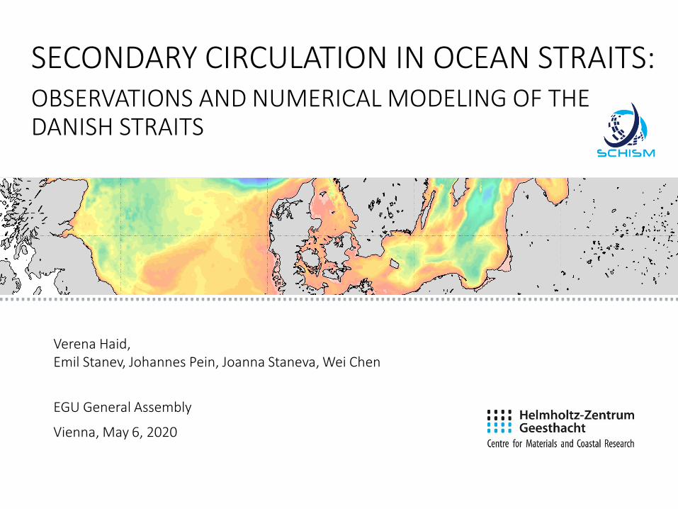
SECONDARY CIRCULATION IN OCEAN STRAITS:

Verena Haid,Emil Stanev, Johannes Pein, Joanna Staneva, Wei Chen

EGU General Assembly

Vienna, May 6, 2020

OBSERVATIONS AND NUMERICAL MODELING OF THE DANISH STRAITS

PREFACESecondary Circulation in Ocean straits

2

Welcome and thank you for your interest!

We all know that these are extraordinary times and while this presentation was planned to be an oral presentation, I tried to add all the necessary information. However, should you find something missing or are interested in more detail, please know that our publication

Haid et al., 2020, Secondary circulation in shallow ocean straits: Observations and numerical modeling of the Danish Straits. Ocean Modelling 148, 101585. https://www.sciencedirect.com/science/article/pii/S1463500319303099?via%3Dihub

will provide you with further facts.

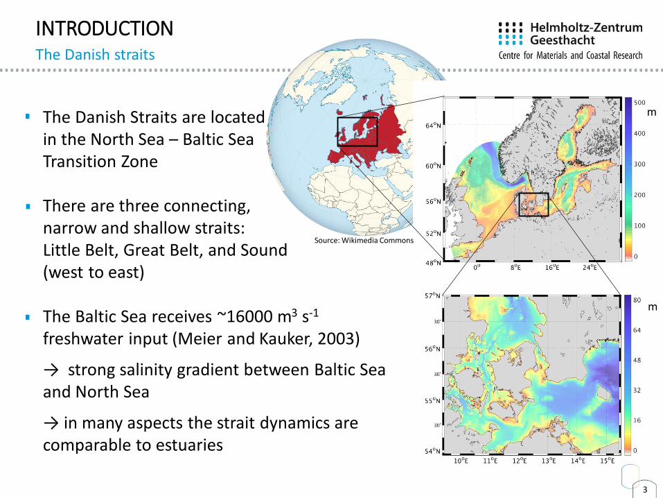
INTRODUCTIONThe Danish straits

3

m

The Danish Straits are located in the North Sea – Baltic Sea Transition Zone

There are three connecting, narrow and shallow straits:Little Belt, Great Belt, and Sound(west to east)

The Baltic Sea receives ~16000 m3 s-1

freshwater input (Meier and Kauker, 2003)

→ strong salinity gradient between Baltic Sea and North Sea

→ in many aspects the strait dynamics are comparable to estuaries

m

Source: Wikimedia Commons

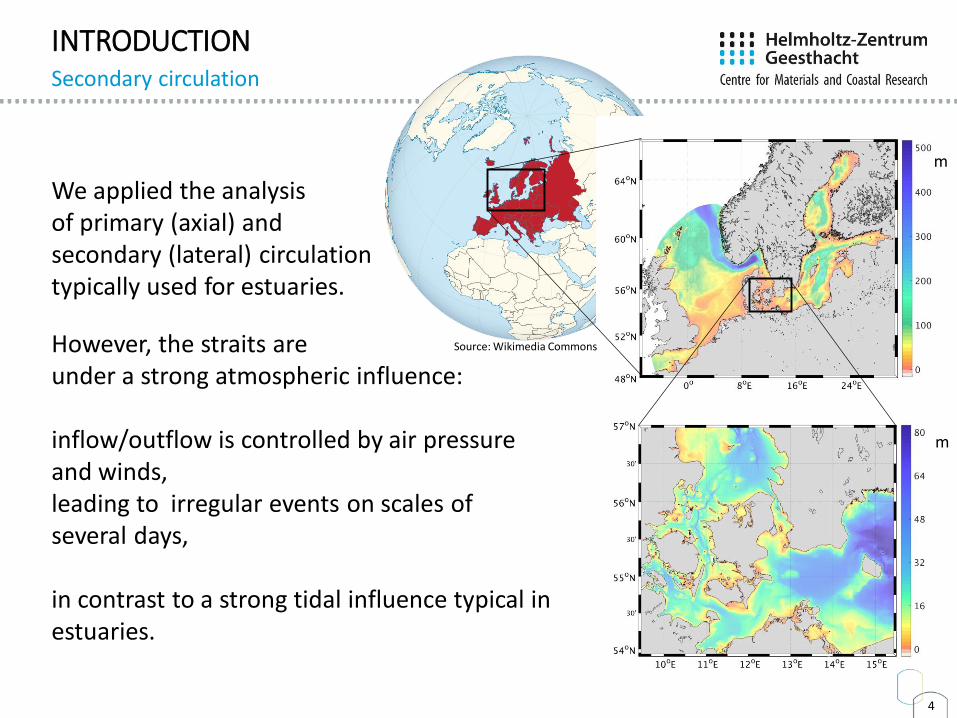
INTRODUCTIONSecondary circulation

4

m

We applied the analysisof primary (axial) and secondary (lateral) circulation typically used for estuaries.

However, the straits are under a strong atmospheric influence:

inflow/outflow is controlled by air pressure and winds, leading to irregular events on scales of several days,

in contrast to a strong tidal influence typical in estuaries.

m

Source: Wikimedia Commons

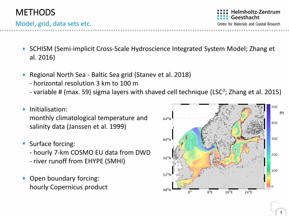
METHODSModel, grid, data sets etc.

5

SCHISM (Semi-implicit Cross-Scale Hydroscience Integrated System Model; Zhang et al. 2016)

Regional North Sea - Baltic Sea grid (Stanev et al. 2018) - horizontal resolution 3 km to 100 m - variable # (max. 59) sigma layers with shaved cell technique (LSC2; Zhang et al. 2015)

Initialisation: monthly climatological temperature and salinity data (Janssen et al. 1999)

Surface forcing: - hourly 7-km COSMO EU data from DWD- river runoff from EHYPE (SMHI)

Open boundary forcing: hourly Copernicus product

m

O-V

O-D

50

100

150

T-SA

O-V

O-D100

150

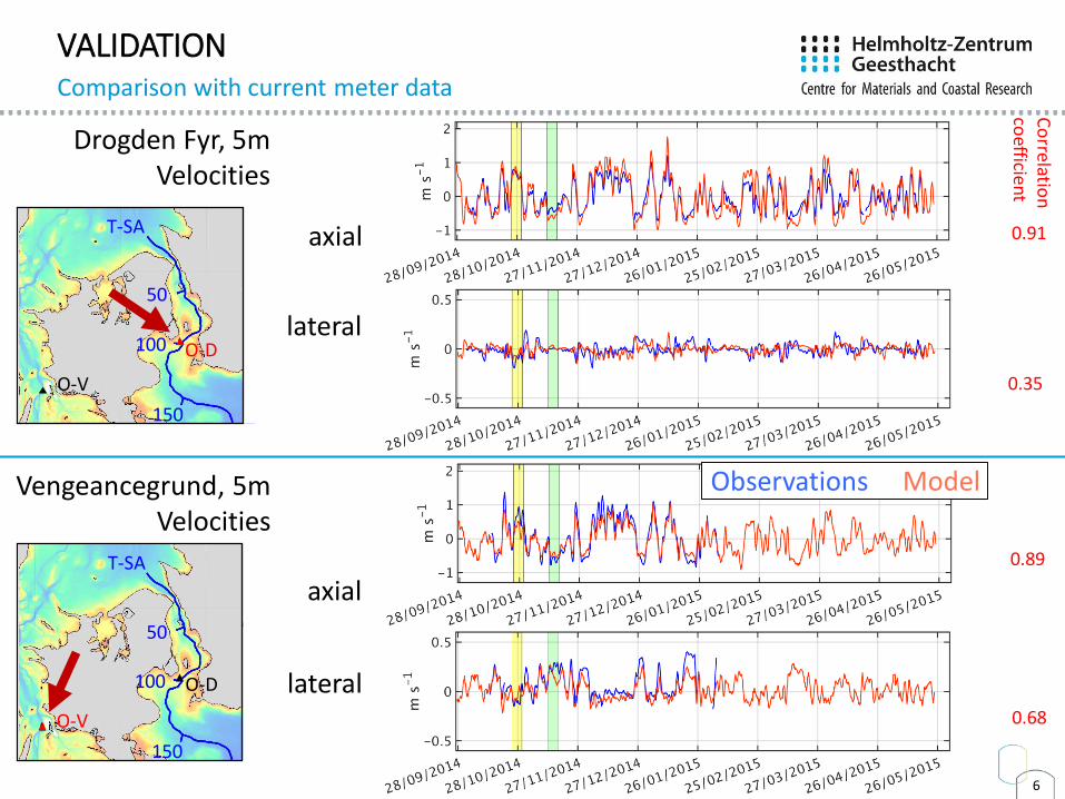
Drogden Fyr, 5mVelocities

lateral

VALIDATIONComparison with current meter data

6

Vengeancegrund, 5mVelocities

lateral

Observations Model

0.91

axial

axial

0.89

0.35

0.68

Co

rrelation

co

efficient

50

T-SA

VALIDATIONComparison with current meter data

7

Current observations of the necessary duration are sparse and we arelucky to have two stations to compare with.

At both stations, the model shows very good agreement for the axial flowwith a correlation coefficient close to 0.9.

For the lateral flow, the station in the Great Belt (Vengeancegrund) showsa good performance with a correlation coefficient of 0.68.

The comparatively low correlation for lateral flow in the Sound is due tothe station‘s location in a very shallow area (Drogden Sill, 8 m depth), where the water is well mixed and thus secondary circulation is weak. The signal-to-noise ratio at this station (Drogden Fyr) is very high.

In the following, we will examine the secondary circulation in the Sound at different locations.

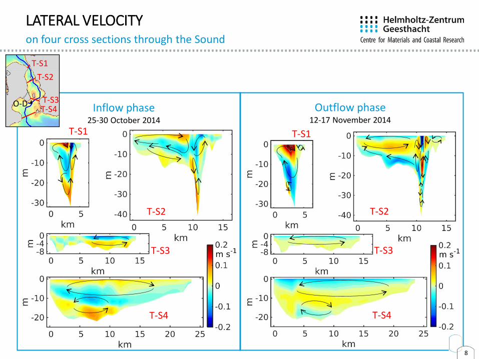
LATERAL VELOCITYon four cross sections through the Sound

T-S1

T-S2

T-S4

T-S3

T-S1

T-S2

T-S4

T-S3

Inflow phase25-30 October 2014

Outflow phase12-17 November 2014

8

T-S1

T-S2

T-S3T-S4

O-D

LATERAL VELOCITYon four cross sections through the Sound

9

The patterns of the secondary circulation are strongly determined bytopography and position in the strait. Also, inflow and outflow will not necessarily generate opposing circulation patterns.

On the northern end of the Sound, the influence of the high salinityNorth Sea water makes itself known during the inflow phase. T-S1 andTS-2 show features reminiscent of the textbook case of differential advection in an estuary during flood.

However, the interplay with other influences (Coriolis force, streamlinecurvature, advected lateral momentum) complicates the apparentpatterns of the secondary circulation.

T-S1 and T-S2 also feature the highest lateral velocities. At the shallow T-S3 transect they are lowest. This is in keeping with the missing ‚signal‘ at the observation station Drogden Fyr.

DIFFERENCES TO ESTUARINE CIRCULATIONAlong-channel transect T-SA

10

inflow outflowSalinity

Richardson number

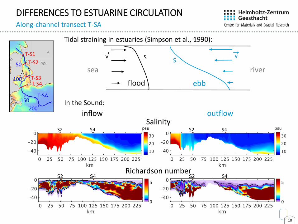
Tidal straining in estuaries (Simpson et al., 1990):

sea river

flood

Sv

ebb

SvT-S1

T-S2

T-S3T-S4

50

100

T-SA150

200In the Sound:

DIFFERENCES TO ESTUARINE CIRCULATIONAlong-channel transect T-SA

11

In a transect along the strait, we find interesting features unknown fromestuaries.In contradiction to tidal straining in estuaries, (where the flood tends toweaken the water column stability and during ebb the surface flow offresh water has a stabilizing effect,) in the Sound the water columnappears well mixed during the outflow phase and gradient Richardson numbers are lower than during the inflow phase.

There are several reasons why the behaviour differs from estuaries:Inflow and outflow phases are of irregular duration and intensity. In thepresented case e.g. the outflow velocities are twice as fast, secondarycirculation and mixing is therefore enhanced. The phases last for several days (the figure shows a 6-day mean). Time enough to flush a large portion of the strait and move the salinity front by75 km.The geometry of a strait typically features one or more narrow and/orshallow constricting areas in the middle and widen toward both ends, while an estuary typically widens toward the sea.

INFLUENCE OF MODEL RESOLUTIONTransect T-S2, lateral velocity

Grid resolution Lateral velocity

Up to 500 m

Up to 100 m

T-S1

T-S2

T-S3

T-S4

O-D50

100

COARSE

FINEf)

outflowinflow

12

INFLUENCE OF MODEL RESOLUTIONTransect T-S2, lateral velocity

13

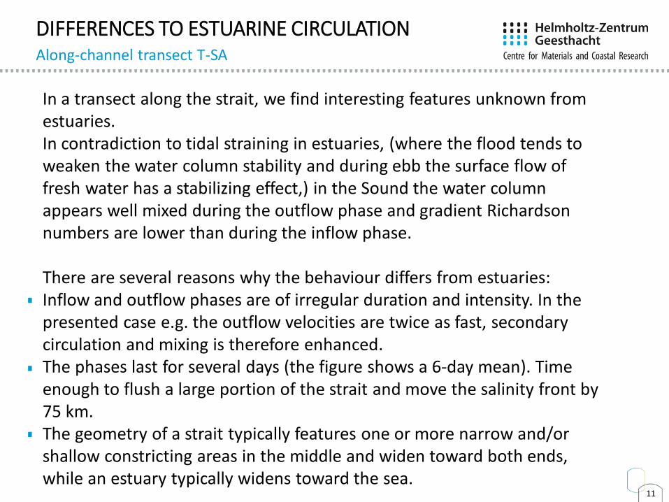
How important is it to adequately resolve the secondary circulationin straits (and what is an adequate resolution)?

Comparing the previously presented experiment (FINE, up to 100 m horizontal resolution) with an experiment with a minimumresolution of 500 m (COARSE), we find that in COARSE thecomplexity of the secondary circulation is much reduced as smallercirculation cells cannot be resolved. This entails an underestimationof lateral (and vertical) velocities and therefore mixing.

COARSE

14

INFLUENCE OF MODEL RESOLUTIONTransect T-SA, along-channel characteristics

T-S1

T-S2

T-S3T-S4

50

100

T-SA150

200 FINE

inflow outflow

Salinity

15

INFLUENCE OF MODEL RESOLUTIONTransect T-SA, along-channel characteristics

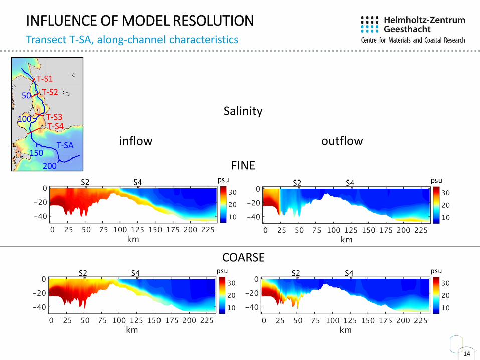
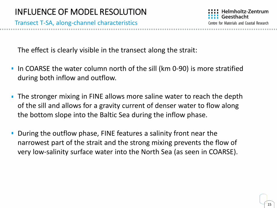
The effect is clearly visible in the transect along the strait:

In COARSE the water column north of the sill (km 0-90) is more stratifiedduring both inflow and outflow.

The stronger mixing in FINE allows more saline water to reach the depthof the sill and allows for a gravity current of denser water to flow alongthe bottom slope into the Baltic Sea during the inflow phase.

During the outflow phase, FINE features a salinity front near thenarrowest part of the strait and the strong mixing prevents the flow ofvery low-salinity surface water into the North Sea (as seen in COARSE).

16

INFLUENCE OF MODEL RESOLUTIONTransect T-S2, two-directional transport

T-S1

T-S2

T-S3T-S4

O-V

O-D50

100

150

T-SA

Two-directional transport

FINE COARSE

----- FINE- - - COARSE

17

INFLUENCE OF MODEL RESOLUTIONTransect T-S2, two-directional transport

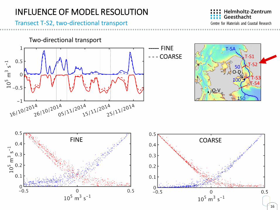
These changes also affect the axial flow through the strait.

Volume transport is higher in FINE since a fully developed secondarycirculation allows for an easier momentum transfer from axial to lateral direction, and back, when the flow navigates the complex geometry ofthe strait (Pein et al., 2018).

Not only peak transports are higher in FINE, also the two-directionaltransports are strengthened at T-S2. The inflow of saline water is higher, which is compensated with an increased counter-flow of fresher water(and vice versa for the outflow phase).

SUMMARY AND CONCLUSIONSSecondary circulation in ocean straits

18

Position and topography exert a strong influence on the appearance of the secondary circulation, which differs strongly with location

Circulation differs from estuarine circulation due to- Irregularity of forcing- Net inflow of comparable magnitude as two-way exchange flow- Different geometry (two-way funnel)- Longer time scales

Inadequate resolution leads to-> misrepresentation of secondary circulation cells-> underestimation of vertical and horizontal mixing -> biased axial flow, water characteristics and transports

For further details:Haid et al., 2020, Secondary circulation in shallow ocean straits: Observations and numerical modeling of the Danish Straits. Ocean Modelling 148, 101585.DOI: 10.1016/j.ocemod.2020.101585