Second-Order Type Optimization AlgorithmsFor Machine Learning

Zaiwen Wen

Beijing International Center For Mathematical ResearchPeking University

1/47

2/47

References/Coauthors in our group or alumnus

(a) Andre (b) 李勇锋 (c) 柳伊扬 (d) 陈子昂 (e) 赵明明 (f) 杨明瀚

Li Yongfeng, Wen Zaiwen, Yang Chao, Yuan Yaxiang; A Semi-smooth Newton MethodFor semidefinite programs and its applications in electronic structure calculations;SIAM Journal on Scientific ComputingChen Ziang, Andre Milzarek, Wen Zaiwen; A Trust-Region Method For NonsmoothNonconvex Optimization, arXiv: 2002.08513Andre Milzarek, Xiao Xiantao, Cen Sicong, Wen Zaiwen, Michael Ulbrich; A stochasticsemi-smooth Newton method for nonsmooth nonconvex optimization, SIAMJournal on OptimizationYang Minghan, Andre Milzarek, Wen Zaiwen, Zhang Tong, Stochastic semi-smoothQuasi-Newton method for nonsmooth optimizationZhao Mingming, Li Yongfeng, Wen Zaiwen, A stochastic trust region framework forpolicy optimization

3/47

Outline

1 Basic Concepts of Semi-smooth Newton method

2 A Trust Region Method For Nonsmooth Convex Programs

3 Stochastic Semi-smooth Newton Methods

4 A stochastic trust region method for deep reinforcement learning

4/47

Composite convex program

Consider the following composite convex program

minx∈Rn

f (x) + ϕ(x),

where f and h are convex, f is differentiable but h may not

Many applications:Sparse and low rank optimization: h(x) = ‖x‖1 or ‖X‖∗ and manyother forms.

Regularized risk minimization: f (x) =∑

i fi(x) is a loss function ofsome misfit and ϕ is a regularization term.

Constrained program: ϕ is an indicator function of a convex set.

5/47

A General Recipe

Goal: study approaches to bridge the gap between first-order andsecond-order type methods for composite convex programs.

key observations:Many popular first-order methods can be equivalent to somefixed-point iterations: xk+1 = T(xk);

Advantages: easy to implement; converge fast to a solution withmoderate accuracy.

Disadvantages: slow tail convergence.

The original problem is equivalent to the systemF(x) := (I − T)(x) = 0.

Newton-type method since F(x) is semi-smooth in many cases

Computational costs can be controlled reasonably well

6/47

An SDP From Electronic Structure Calculation

system: BeO

0 1000 2000 3000 4000 5000 6000 7000

iter

10-8

10-6

10-4

10-2

100

102

err

(g) ADMM

2000 2010 2020 2030 2040 2050 2060 2070

iter

10-8

10-6

10-4

10-2

100

err

(h) Semi-smooth Newton

7/47

Proximal gradient method

A first-order method

xk+1 = arg minx

⟨∇f (xk), x− xk⟩+

λ

2‖x− xk‖2

2 + ϕ(x)

= proxλϕ(xk −∇f (xk)/λ

), k = 0, 1, · · · ,

where the proximal mapping is:

proxλϕ(x) := argminu∈Rn

ϕ(u) +λ

2‖u− x‖2

2.

Equivalent to find a root of a fixed-point mapping

x = T(x) = proxλϕ(x−∇f (x)/λ)

8/47

Semi-smoothness

Solving the systemF(z) = 0,

where F(z) = T(z)− z and T(z) is a fixed-point mapping.

F(z) fails to be differentiable in many interesting applications.

but F(z) is (strongly) semi-smooth and monotone.(a) F is directionally differentiable at x; and

(b) for any d ∈ Rn and J ∈ ∂F(x + d),

‖F(x + d)− F(x)− Jd‖2 = o(‖d‖2) as d → 0.

9/47

A regularized semi-smooth Newton method

The Jacobian Jk ∈ ∂BF(zk) is positive semidefinite

Let µk = λk‖Fk‖2. Constructe a Newton system:

(Jk + µkI)d = −Fk,

Solving the Newton system inexactly:

rk := (Jk + µkI)dk + Fk.

We seek a step dk approximately such that

‖rk‖2 ≤ τ min1, λk‖Fk‖2‖dk‖2, where 0 < τ < 1

Newton Step: zk+1 = zk + dk

Faster local convergence is ensured

10/47

Semidefinite Programming

Consider the SDP

min 〈C,X〉 , s.t. AX = b,X 0

f (X) = 〈C,X〉+ 1AX=b(X).

h(X) = 1K(X), where K = X : X 0.

Proximal Operator: proxth(Z) = arg minX12‖X − Z‖2

F + th(X)

Let Z = QΣQT be the spectral decomposition

proxtf (Y) = (Y + tC)−A∗(AY + tAC − b),

proxth(Z) = QαΣαQTα,

Fixed-point mapping from DRS:

F(Z) = proxth(Z)− proxtf (2proxth(Z)− Z) = 0.

11/47

Semi-smooth Newton System

assumption: AA∗ = I

The SMW theorem yields the inverse matrix

(Jk + µkI)−1 = H−1 + H−1AT(I − AWH−1AT)−1AWH−1

=1

µ(µ+ 1)(µI + T)(I + A>(

µ2

2µ+ 1I + ATA>)−1A(

µ

2µ+ 1I − T)).

ATA>d = AQ(Ω0 (QT(D)Q))QT , where D = A∗d,

Ω0 =

[Eαα lααlTαα 0

],

and Eαα is a matrix of ones and lij =µkij

µ+1−kij

computational cost O(|α|n2)

12/47

Comparison on electronic structure calculation

0 2 4 6 8

not more than 2 x times worse than the best

0

0.2

0.4

0.6

0.8

1

ratio

of

pro

ble

ms

maxp,

d,

g

SDPNAL

SDPNAL+

SSNSDP

(i) max(ηp,ηd,ηg)

0 1 2 3 4

not more than 2 x times worse than the best

0

0.2

0.4

0.6

0.8

1

ratio o

f pro

ble

ms

cpu

SDPNAL

SDPNAL+

SSNSDP

(j) cpu time

13/47

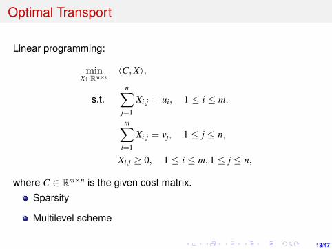
Optimal Transport

Linear programming:

minX∈Rm×n

〈C,X〉,

s.t.n∑

j=1

Xi,j = ui, 1 ≤ i ≤ m,

m∑i=1

Xi,j = vj, 1 ≤ j ≤ n,

Xi,j ≥ 0, 1 ≤ i ≤ m, 1 ≤ j ≤ n,

where C ∈ Rm×n is the given cost matrix.Sparsity

Multilevel scheme

14/47

Squared `2-DOTmark 128× 128 images

MSSN CPLX-NWS M-CPLXClass TIME/SSN/CG gap/pinf/dinf TIME TIME

WhiteNoise 24.86/1717/18839 3.57e-07/9.90e-07/2.98e-08 1262.96 22.09GRFrough 21.61/1375/12727 2.00e-07/7.28e-07/4.20e-08 1398.86 53.71GRFmod 18.28/1049/8573 1.14e-09/9.69e-07/1.19e-07 1703.69 51.16

GRFsmooth 35.15/1467/17149 1.79e-08/9.86e-07/3.45e-08 1892.41 69.25LogGRF 94.41/3945/22768 2.23e-10/9.93e-07/7.83e-07 2066.44 56.17LogitGRF 83.57/3276/33599 1.31e-08/8.96e-07/9.57e-07 1928.92 83.84Cauchy 104.64/17826/256255 1.86e-07/9.65e-07/9.34e-07 1869.37 51.30Shapes 9.12/748/3380 1.19e-08/5.67e-07/3.38e-10 2501.76 12.11Classic 31.73/2820/27321 1.18e-07/7.45e-07/3.27e-07 1732.93 70.36

Microscopy 24.69/1663/10880 8.52e-09/9.98e-07/9.30e-08 1671.90 35.14

15/47

Outline

1 Basic Concepts of Semi-smooth Newton method

2 A Trust Region Method For Nonsmooth Convex Programs

3 Stochastic Semi-smooth Newton Methods

4 A stochastic trust region method for deep reinforcement learning

16/47

Problem setup

Nonsmooth composite program:

minx∈Rn

ψ(x) := f (x) + ϕ(x),

where f : Rn → R is a (probably nonconvex) smooth function andϕ : Rn → R is a convex, proper, and lower semi-continuousmapping.Trust-region subproblem:

mins∈Rn

mk(p) = ψk + gTk p +

12

pTBkp, s.t. ‖p‖ ≤ ∆k.

g(x) is an extension of the gradient and will be constructed later.A desired property: mk(p) locally fits ψ(x) well along a specificdirection.

17/47

Construction of g(x)

The steepest descent direction: ds(x) = argmind∈Rn, ‖d‖≤1

ψ′(x; d).

In the smooth case: ∇ψ(x) = ψ′(x; ds(x))ds(x).In the nonsmooth case, we choose a descent direction d(x) with

‖d(x)‖ =

0, 0 ∈ ∂ψ(x),

1, 0 /∈ ∂ψ(x),

and an upper bound of the directional derivative:

u(x) ∈

[ψo(x, d(x)), 0), 0 /∈ ∂ψ(x),

0, 0 ∈ ∂ψ(x).

g(x) := u(x)d(x).

18/47

Preferable Choices of d(x) and u(x)

Choice 1:We say dγ(x) is a γ-inexact steepest descent direction (γ ∈ (0, 1])if it satisfies ‖dγ(x)‖ ≤ 1 and ψ′(x; dγ(x)) ≤ γψ′(x; ds(x)).d(x) = dγ(x), u(x) = ψ′(x; dγ(x)).Choice 1 may be difficult to implement.

Choice 2:

Proximal Operator: proxΛϕ(x) := argmin

z∈Rnϕ(z) +

12‖z− x‖2

Λ.

Natural Residual: FΛnat(x) := x− proxΛ

ϕ(x− Λ−1∇f (x)).A point x∗ is a stationary point of problem (16) if and only if x∗ is asolution of the nonsmooth equation FΛ

nat(x) = 0.

ψ′(x;−FΛ

nat(x))≤ −

∥∥FΛnat(x)

∥∥2Λ

.

d(x) = − FΛnat(x)

‖FΛnat(x)‖ , u(x) = −λmin

∥∥FΛnat(x)

∥∥.

19/47

Model Function and Trust-Region Subproblem

Let gk = u(xk)d(xk). Trust region subproblem:

mins

mk(s) = ψk + 〈gk, s〉+12〈s,Bks〉 s.t. ‖s‖ ≤ ∆k

Cauchy point: pCk := −αC

k gk and αCk := argmin

0≤t≤ ∆k‖gk‖

mk(−tgk).

Choose the regularization parameter:

12

hTBkh + tk‖h‖2 ≥ λ1‖h‖2 ∀ h ∈ Rn and ‖Bk + tkI‖ ≤ λ2,

Solve a system: (Bk + tkI)p = −gk such that

(Bk + tkI)pk = −gk + rk and ‖rk‖ ≤ λ1

2(λ1 + λ2)‖gk‖.

Project pk onto the trust region: sk = min∆k, ‖pk‖pk

20/47

Suitable Stepsize

Descent direction pk = pk‖pk‖ .

Γmax(x, d) := sup

T > 0 : ψox,d(t) := ψo(x + td; d) ∈ C(0,T)

Γ(x) := infd∈Rn, ‖d‖=1 Γmax(x, d)

Stepsize αk = min Γ (xk; pk) , ‖pk‖.Example: n = 2, ϕ(x) = ‖x‖1, where qk := αkpk.

21/47

Truncation Step

Definition 1If there exists a sequence Sim

i=0 satisfying Rn = S0 ⊃ S1 · · · ⊃ Sm,δ ∈ (0,+∞], κ > 0, and a function T : Rn × (0, δ]→ Rn with followingproperties:(1) Γ(x) ≥ δ, ∀x ∈ Sm;(2) For any a ∈ (0, δ] and x ∈ Si\Si+1 (i ∈ 0, 1, · · · ,m− 1), if Γ(x) ≥ a, itholds T(x, a) = x; if Γ(x) < a, it holds T(x, a) ∈ Si+1, Γ(T(x, a)) ≥ a,and ‖T(x, a)− x‖ ≤ κa;we say ϕ is truncatable and T is a truncation operator.

22/47

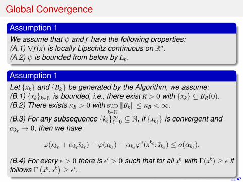
Global Convergence

Assumption 1We assume that ψ and f have the following properties:(A.1) ∇f (x) is locally Lipschitz continuous on Rn.(A.2) ψ is bounded from below by Lb.

Assumption 1Let xk and Bk be generated by the Algorithm, we assume:(B.1) xkk∈N is bounded, i.e., there exist R > 0 with xk ⊆ BR(0).(B.2) There exists κB > 0 with sup

k∈N‖Bk‖ ≤ κB <∞.

(B.3) For any subsequence k`∞`=0 ⊆ N, if xk` is convergent andαk` → 0, then we have

ϕ(xk` + αk` sk`)− ϕ(xk`)− αk`ϕo(xk` ; sk`) ≤ o(αk`).

(B.4) For every ε > 0 there is ε′ > 0 such that for all xk with Γ(xk) ≥ ε itfollows Γ

(xk, sk

)≥ ε′.

23/47

Global Convergence

Theorem 1For truncatable ϕ, suppose that (A.1), (A.2), (B.1)-(B.4) are satisfied.Assume that the Algorithm does not terminate in finitely many stepsand let xk∞k=0 be the sequence generated by the Algorithm. Then itholds that

lim infk→∞

‖gk‖ = 0.

Theorem 1Under the same assumptions as in the last Theorem, let x∗ be anyaccumulation point of the sequence xk∞k=0 generated by theAlgorithm where gk is given by Choice 1 or Choice 2. Then x∗ is anstationary point of (16).

24/47

Outline

1 Basic Concepts of Semi-smooth Newton method

2 A Trust Region Method For Nonsmooth Convex Programs

3 Stochastic Semi-smooth Newton Methods

4 A stochastic trust region method for deep reinforcement learning

25/47

Stochatic optimization problem

Considerminx∈Rn

Ψ(x) := f (x) + ϕ(x)

Expected and Empirical Risk Minimization:

f (x) := E[F(x, ξ)], f (x) =1N

N∑i=1

fi(x)

Assume f (x) is smooth but ϕ(x) is convex and non-smooth.Large-scale machine learning problems: the number of datasamples N is very largeFull evaluation of f (x) and ∇f (x) is not tractable or simply tooexpansive.

26/47

Algorithmic Idea

Basic idea based on xk+1 = proxλϕ(xk − t∇f (xk)).We incorporate second order information and use stochasticHessian oracles (SSO)

Htk(xk) ≈ ∇2f (xk)

to estimate the Hessian ∇2f and compute the Newton step.The sample collections sk and tk are chosen independently ofeach other and of the other batches s`, t`, ` ∈ N0 \ k.

We work with the following SFO and SSO:

∇fsk(x) :=1|sk|

∑i∈sk

∇fi(x) and Htk(x) :=1|tk|∑i∈tk∇2fi(x).

27/47

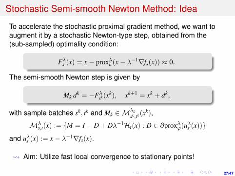
Stochastic Semi-smooth Newton Method: Idea

To accelerate the stochastic proximal gradient method, we want toaugment it by a stochastic Newton-type step, obtained from the(sub-sampled) optimality condition:

Fλs (x) = x− proxλh (x− λ−1∇fs(x)) ≈ 0.

The semi-smooth Newton step is given by

Mk dk = −Fλsk(xk), xk+1 = xk + dk,

with sample batches sk, tk and Mk ∈Mλksk,tk(xk),

Mλs,t(x) := M = I − D + Dλ−1Ht(x) : D ∈ ∂proxλϕ(uλs (x))

and uλs (x) := x− λ−1∇fs(x).

Aim: Utilize fast local convergence to stationary points!

28/47

Algorithmic Framework

We use the following growth conditions (?):

‖Fλk+1sk+1 (zk)‖ ≤ (η + νk) · θk + ε1

k , (G.1)

ψ(zk) ≤ ψ(xk) + β · θ1/2k ‖F

λk+1sk+1 (zk)‖1/2 + ε2

k , (G.2)

where η ∈ (0, 1), β > 0, and (νk), (ε2k) ∈ `1

+, (ε1k) ∈ `1/2

+ .

We set θk+1 to ‖Fλk+1sk+1 (xk+1)‖ if xk+1 was obtained in step 3.

Remark:

Calculating Fλk+1sk+1 (zk) requires evaluation of ∇fsk+1(zk). This

information can be reused in the next iteration if zk xk+1 isaccepted as new iterate.

29/47

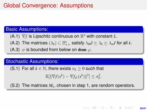
Global Convergence: Assumptions

Basic Assumptions:(A.1) ∇f is Lipschitz continuous on Rn with constant L.(A.2) The matrices (λk) ⊂ Sn

++ satisfy λMI λk λmI for all k.(A.3) ψ is bounded from below on dom ϕ.

Stochastic Assumptions:(S.1) For all k ∈ N, there exists σk ≥ 0 such that

E[‖∇f (xk)−∇fsk(xk)‖2] ≤ σ2k .

(S.2) The matrices Mk, chosen in step 1, are random operators.

30/47

Global Convergence

Theorem: Global Convergence [MXCW, ’17]

Suppose that (A.1)–(A.3) and (S.1)–(S.2) are fulfilled. Then, underthe additional conditions, αk ≤ α := min1, λm/L,

(αk) is nonincreasing ,∑

αk =∞,∑

αkσ2k <∞

it holds lim infk→∞ E[‖Fλ(xk)‖2] = 0 and lim infk→∞ Fλ(xk) = 0 a.s. forany λ ∈ Sn

++.

Verify that (xk) actually defines an adapted stochastic process.The batch sk and the iterate xk are not independent.Derive approximate and uniform descent estimates for the termsψ(xk)− ψ(xk+1).

For strongly convex case: limk→∞ E[‖Fλ(xk)‖2] = 0 andlimk→∞ Fλ(xk) = 0 a.s. for any λ ∈ Sn

++.

31/47

Stochastic Semi-smooth Quasi-Newton Method

Use stochastic approximation technique!Estimate vk ≈ ∇f (xk) from stochastic oracle and set

Fvk(xk) := xk − proxλϕ(xk − vk/λ).

Example: Assume the samples s are chosen independently, thena possible estimate of ∇f (x) is ∇fs(xk) := 1

|s|∑

i∈s∇fi(xk).

Use extra-gradient step for globalization!(a) First employ the “Newton” step:

zk = xk + βkdk, dk = −WkFvk (xk)

where Wk is exact or approximation of inverse of Jk.

(b) Perform an extra gradient step:

xk+1 = proxλϕ(xk + αkdk − vk+/λ), vk

+ ≈ ∇f (zk).

The choice of βk and αk are very flexible !

32/47

Coordinate Quasi-Newton Method

Further computation reduction?Use coordinate update!Given a coordinates set A(xk) and O(xk) := [N] \ A(xk), dk isupdated by coordinate set:

dk = −

WA(xk)A(xk) 0

0 γkI

(Fλvk(xk))A(xk)

(Fλvk(xk))O(xk)

,WA(xk)A(xk) is updated by L-BFGS related to coordinates A(xk).

(Uk)A(xk) = [uk−pA(xk)

, . . . , uk−1A(xk)

], (Yk)A(xk) = [yk−pA(xk)

, . . . , yk−1A(xk)

],

are the subvectors of Uk,Yk.

33/47

Convergence Assumption

Basic AssumptionA.1 The gradient mapping ∇f is Lipschitz continuous on Rn with modulus Lf ≥ 1.

A.2 The objective function ψ is bounded from below on dom ϕ.

A.3 ϕ : Rn → (−∞,∞] is convex, lower semicontinuous, and proper.

Stochastic Assumption

B.1 The mapping Dk : Ω→ Rn is an F k-measurable function for all k.

B.2 There is νk > 0 such that we have E[‖Dk‖2 | F k−1+ ] ≤ ν2

k · E[‖FVk (Xk)‖2 | F k−1+ ]

a.e. and for all k ∈ N.

B.3 For all k ∈ N, it holds E[Vk | F k−1+ ] = ∇f (Xk), E[Vk

+ | F k] = ∇f (Zk) a.e. andthere exists σk, σk,+ > 0 such that a.e.

E[‖∇f (Xk)− Vk‖2 | F k−1+ ] ≤ σ2

k and E[‖∇f (Zk)− Vk+‖2 | F k] ≤ σ2

k,+,

whereF k = σ(V0,V0

+, . . . ,Vk) and F k

+ = σ(Fk ∪ σ(Vk+)).

34/47

Theorem 1

Suppose that the assumptions (A.1)–(A.3) and (B.1)–(B.3) aresatisfied and we have

λk,+ ≤1Lf, λk ≤

(1− ρ)λk,+

1 + µ2k

,

where µk = νk(αk + Lfβkλk,+). Then, under the additional conditions∑λk =∞,

∑λkσ

2k <∞,

∑λk,+σ

2k,+ <∞

it follows lim infk→∞ E[‖F(Xk)‖2] = 0 and lim infk→∞ F(Xk) = 0 a.s.and (ψ(Xk))k a.s. converges to some random variable Y∗ withlimk→∞ E[ψ(Xk)] = E[Y∗].

Locally, if we further assume the function satisfy KL-property andsome mild assumption, we can show then (Xk)k converges almostsurely to a crit ψ-valued random variable X∗.

35/47

Deep learning: ResNet-18 on Cifar10, ψ(x) = ‖x‖1

0 25 50 75 100 125 150 175 200Epoch

10

20

30

40

50

60

70

80

90

100

Training

Acc

Prox-SGDSEQN

(a) Training accuracy

0 25 50 75 100 125 150 175 200Epoch

10

20

30

40

50

60

70

80

90

100

Testing Acc

Prox-SGDSEQN

(b) Testing accuracy

36/47

Outline

1 Basic Concepts of Semi-smooth Newton method

2 A Trust Region Method For Nonsmooth Convex Programs

3 Stochastic Semi-smooth Newton Methods

4 A stochastic trust region method for deep reinforcement learning

37/47

Reinforcement learning

38/47

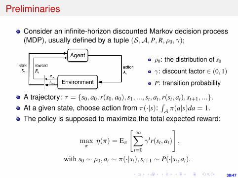
Preliminaries

Consider an infinite-horizon discounted Markov decision process(MDP), usually defined by a tuple (S,A,P,R, ρ0, γ);

ρ0: the distribution of s0

γ: discount factor ∈ (0, 1)

P: transition probability

A trajectory: τ = s0, a0, r(s0, a0), s1, ..., st, at, r(st, at), st+1, ....At a given state, choose action from π(·|s):

∫A π(a|s)da = 1.

The policy is supposed to maximize the total expected reward:

maxπ

η(π) = Eπ

[ ∞∑t=0

γtr(st, at)

],

with s0 ∼ ρ0, at ∼ π(·|st), st+1 ∼ P(·|st, at).

39/47

Deep reinforcement learning

In real-world tasks: high dimensionality, limited observations,...In deep reinforcement learning, the policy π and/or valuefunctions are usually parameterized with differentiable neuralnetworks.The policy-based optimization:

maxθ

η(θ).

The value-based optimization:

minφ

Es,a

Qφ(s, a)− Es′∼P(·|s,a)

[r(s, a) + γmax

a′Qφ(s′, a′)|s, a

]2

.

Challenges: theoretical analysis; generalization; stability; tradeoff between exploration and exploitation...

40/47

VPG, NPG

Policy gradient: ∇η(θ) = Eρθ,πθ [∇ log πθ(a|s)Aθ(s, a)].

ρθ(s) =∞∑

t=0γtP(st = s|πθ) is the (unnormalized) discounted

visitation frequencies.

Vanilla1/Natural2 policy gradient: θk+1 = θk + αM(θk)∇θη(θk).

M(θk)−1 = Eρθk ,πθk

[∇θ log πθk(s, a)∇θ log πθk(s, a)T

].

A local approximation of η:

η(θ) = η(θk) +∑

s

ρθ(s)∑

a

πθ(a|s)Aθk(s, a),

Lθk(θ) = η(θk) +∑

s

ρθk(s)∑

a

πθ(a|s)Aθk(s, a).

η(θk) = Lθk(θk),∇η(θk) = ∇Lθk(θk).1R. S. Sutton, el al., Policy gradient methods for reinforcement learning with

function approximation.2S. M. Kakade, A natural policy gradient.

41/47

Stochastic Trust Region Algorithm

The objective functionmaxθ

η(θ).

At k-th iteration, obtain a trail point θk+1 from the subproblem:

maxθ

Lθk(θ), s.t. Es∼ρθk[D(πθk(·|s), πθ(·|s))] ≤ δk.

Compute the ratio rk =η(θk+1)−η(θk)

Lθk (θk+1)−Lθk (θk).

Update θk+1 =

θk+1, rk ≥ β0,

θk, o.w.,, with β0 > 0.

Update δk+1 = µk+1‖∇Lθk+1(θk+1)‖ with γ1 > 1 ≥ γ2 > γ3,

µk+1 =

γ1µk, rk ≥ β1,

γ2µk, rk ∈ [β0, β1),

γ3µk, o.w.,

.

42/47

Unparameterized Policy

Specifying the total variation distance in discrete cases (the KLdivergence in continuous cases).

Policy advantage: Aπ(π′) = Es∼ρπ[Ea∼π′(·|s) [Aπ(s, a)]

].

Lemma 2 (Optimality condition)π is the optimal policy if and only if

A∗π = maxπ′

Aπ(π′) = 0, i.e., π ∈ argmaxπ′Aπ(π′).

Lemma 3 (Monotonicity)Suppose πk is the sequence generated by our trust region method,then we have η(πk+1) ≥ η(πk), the equality holds if and only if πk isthe optimal policy.

43/47

Main Results

Lemma 4 (Lower bound of ∆Lπk)Suppose πk is the sequence generated by our trust region method,then we have Lπk(πk+1)− Lπk(πk) ≥ min(1, (1− γ)δk)A∗πk

.

Lemma 5 (Lower bound of rk)

The ratio rk satisfies that rk ≥ min

(1− 4εkγδ

2k

p20(1−γ)2A∗πk

, 1− 4εkγδkp2

0(1−γ)3A∗πk

),

where p0 = mins ρ0(s) and εk = maxs,a |Aπk(s, a)|.

Theorem 6 (Convergence)Suppose πk is the sequence generated by our trust region method,then we have the following conclusions

1 limk→∞

A∗πk= 0.

2 limk→∞

η(πk) = η(π∗), where π∗ is the optimal policy.

44/47

Empirical algorithm

Terminate condition:

|Lθk(θk,l+1)− Lθk(θk,l)|1 +

∣∣Lθk(θk,l)∣∣ ≤ ε, or

|Ent(θk,l+1)− Ent(θk)|1 + |Ent(θk)|

≥ ε.

Ratio:

rk =η(θk+1)− η(θk)

Lθk(θk+1)− Lθk(θk)=⇒ rk =

η(θk+1)− η(θk)

ση(θk) + Lθk(θk+1)− Lθk(θk).

ση(θ) is the empirical standard deviation of η(θ).

Acceptance criteria: θk+1 =

θk+1, rk ≥ β0,

θk, o.w., with a small

negative constant β0 < 0.Mandatory acceptance: after several consecutive rejections,force to accept the best performed point among the pastrejections.

45/47

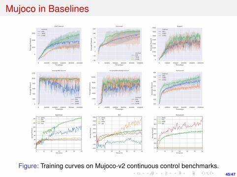
Mujoco in Baselines

0 200000 400000 600000 800000 1000000Timesteps

0

1000

2000

3000

Aver

age

Rewa

rd

HalfCheetahmethodPPOTRPOSTRO

0 200000 400000 600000 800000 1000000Timesteps

50

25

0

25

50

75

100

125

Aver

age

Rewa

rd

Swimmer

methodPPOTRPOSTRO

0 200000 400000 600000 800000 1000000Timesteps

0

500

1000

1500

2000

2500

3000

3500

4000

Aver

age

Rewa

rd

HoppermethodPPOTRPOSTRO

0 200000 400000 600000 800000 1000000Timesteps

0

200

400

600

800

1000

1200

Aver

age

Rewa

rd

InvertedPendulum

methodPPOTRPOSTRO

0 200000 400000 600000 800000 1000000Timesteps

0

2000

4000

6000

8000

10000

Aver

age

Rewa

rd

InvertedDoublePendulum

methodPPOTRPOSTRO

0 200000 400000 600000 800000 1000000Timesteps

100

200

300

400

500

600

700

800

Aver

age

Rewa

rd

HumanoidmethodPPOTRPOSTRO

0 10 20 30 40 50 60Time(min)

0

20

40

60

80

100

120

140

Aver

age

Rewa

rd

SwimmerDDPGTD3STROSAC

0 10 20 30 40 50 60Time(min)

1000

500

0

500

1000

1500

2000

2500

3000

Aver

age

Rewa

rd

AntDDPGTD3STROSAC

0 10 20 30 40 50 60Time(min)

100

200

300

400

500

600

700

Aver

age

Rewa

rd

HumanoidDDPGTD3STROSAC

Figure: Training curves on Mujoco-v2 continuous control benchmarks.

46/47

Atari games

Table: Max Average Reward (100 episodes) ± standard deviation over 5trails of 1e7 time steps.

Environment PPO TRPO STROPong 20±0 3±7 20±0

MsPacman 2125±322 1538±159 2452±487Seaquest 1004±141 692±92 1172±346Bowling 50±17 38±15 105±6Freeway 30±0 28±3 31±0

PrivateEye 100±0 88±16 100±0

47/47

Contact Information

Many Thanks For Your Attention!

北大课程：大数据分析中的算法，华文慕课回放http://bicmr.pku.edu.cn/~wenzw/bigdata2020.html

教材：刘浩洋,户将,李勇锋，文再文，最优化计算方法http://bicmr.pku.edu.cn/~wenzw/optbook.html

Looking for Ph.D students and PostdocCompetitive salary as U.S and Europe

http://bicmr.pku.edu.cn/~wenzw

E-mail: wenzw@pku.edu.cn

Office phone: 86-10-62744125