Embed Size (px)
Citation preview

1
1
Second Order Second Order Measurement System Measurement System
BehaviourBehaviour
2
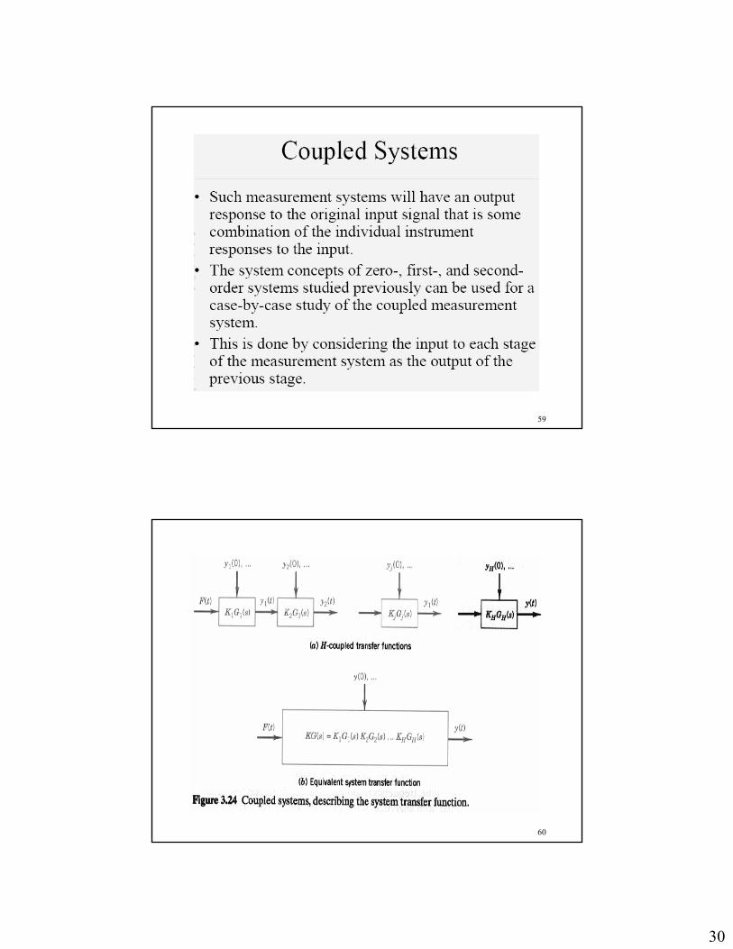
GENERAL MEASUREMENT SYSTEM MODEL
MEASUREMENT SYSTEMMEASUREMENT SYSTEMSYSTEM OUTPUTSYSTEM OUTPUT
y(ty(t))F(tF(t))SIGNAL INPUTSIGNAL INPUT
y(0)y(0)INITIAL CONDITIONSINITIAL CONDITIONS
Understanding the theoretical response of our measurement systemUnderstanding the theoretical response of our measurement system is is essential foressential for
•• Specification of appropriate transducersSpecification of appropriate transducers
•• Understanding our measurement results Understanding our measurement results
However: Exact response is always determined However: Exact response is always determined and confirmed through calibrationand confirmed through calibration

2
3
•• Static measurementStatic measurement: measured physical quantity is NOT : measured physical quantity is NOT changing with timechanging with time
•• Dynamic measurementDynamic measurement: It is ! Consider a vibrating beam : It is ! Consider a vibrating beam –– the the displacement is constantly changing with time. Or fluid flow displacement is constantly changing with time. Or fluid flow under turbulent conditions.under turbulent conditions.
•• We will discuss some important parameters and characteristics We will discuss some important parameters and characteristics applicable to a measurement system under dynamic conditionsapplicable to a measurement system under dynamic conditions
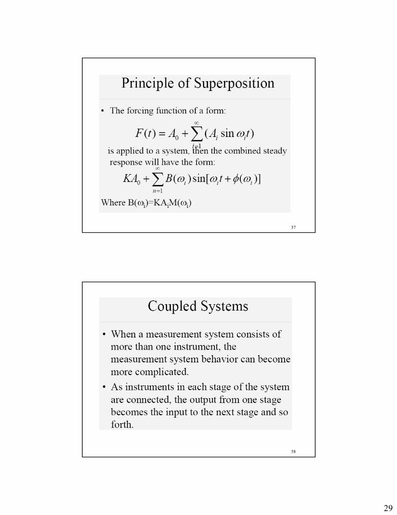
•• A general form of describing a system: A general form of describing a system: through an nthrough an nthth order order nonnon--homogeneous differential equationhomogeneous differential equation
•• The The order of the systemorder of the system is designated by the order of the is designated by the order of the differential equationdifferential equation
•• RightRight--hand side: hand side: Forcing functionForcing function F(tF(t)) imposed on the systemimposed on the system
GENERAL MEASUREMENT SYSTEM MODELGENERAL MEASUREMENT SYSTEM MODEL
4
1.1. ZERO ORDER SYSTEMZERO ORDER SYSTEM
•• General ModelGeneral Model
•• Response to unit step inputResponse to unit step input
2.2. FIRST ORDER SYSTEMFIRST ORDER SYSTEM
•• General Model (recap from temperature unit)General Model (recap from temperature unit)
•• Response to unit step inputResponse to unit step input
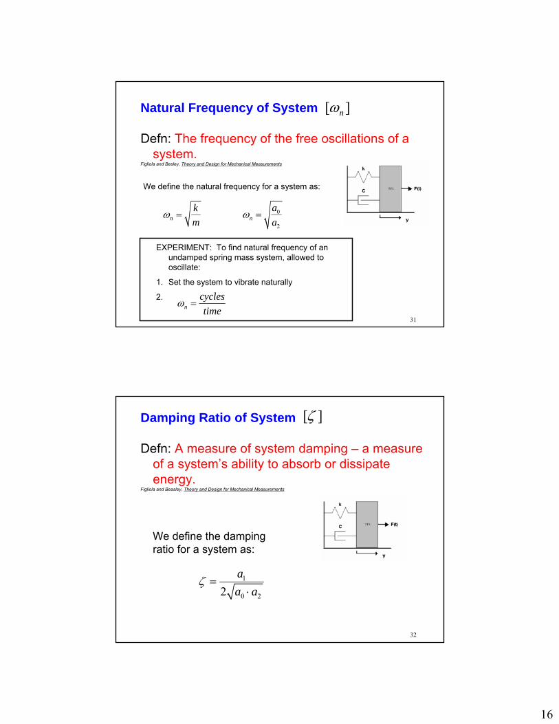
3.3. SECOND ORDER SYSTEMSECOND ORDER SYSTEM
•• General Model General Model
•• Response to unit step inputResponse to unit step input
•• Response to vibration or sinusoidal inputsResponse to vibration or sinusoidal inputs
WE WILL CONSIDER THREE GENERAL SYSTEM MODELSWE WILL CONSIDER THREE GENERAL SYSTEM MODELS

3
5
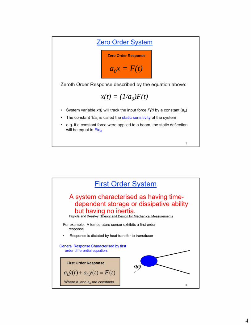
Zero Order System
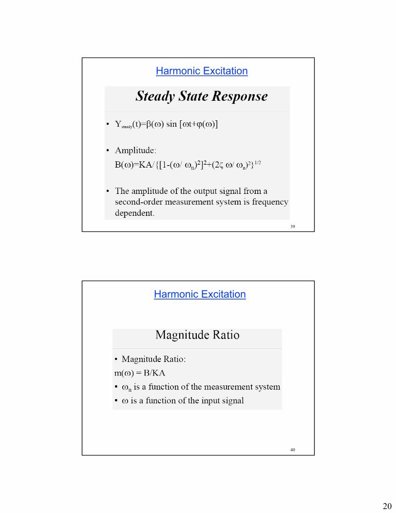
Characteristics of Zero Order System
• Suitable for static signals only
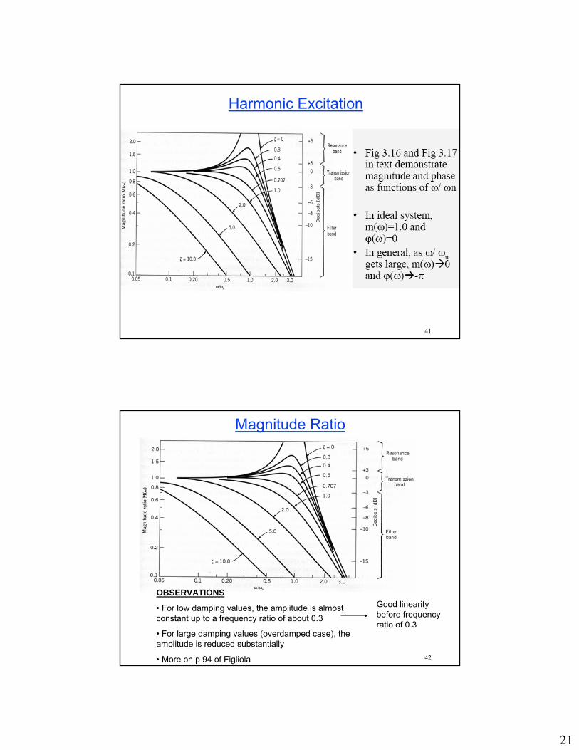
• System has negligible inertia
• System has negligible damping
• Output = constant x input
Defn: A system whose behaviour is independent of the time-dependent characteristics of storage or inertia.
Figliola and Beasley, Theory and Design for Mechanical Measurements
Example: A simple pressure gauge
6
Response of Zero Order System
INPUTRESPONSE
RESPONSE:• Instantaneous response
• Output tracks input exactly
• Characterised by a zeroth order differential equation
Zero Order Response
a0x = F(t)
4
7
Zero Order System
Zeroth Order Response described by the equation above:
x(t) = (1/a0)F(t)
• System variable x(t) will track the input force F(t) by a constant (a0)
• The constant 1/a0 is called the static sensitivity of the system
• e.g. if a constant force were applied to a beam, the static deflection will be equal to F/a0
Zero Order Response
a0x = F(t)
8
First Order Response
First Order System
A system characterised as having time-dependent storage or dissipative ability but having no inertia.
Figliola and Beasley, Theory and Design for Mechanical Measurements
Q(t)
For example: A temperature sensor exhibits a first order response
• Response is dictated by heat transfer to transducer
1 0( ) ( ) ( )a y t a y t F t+ =&
General Response Characterised by first order differential equation:
Where a1 and a0 are constants
5
9
First Order Response to Step Input
INPUT
RESPONSE
0( ) ( )t
y t KA y KA e τ−
= + −
Response of First Order System to Step Input:
Transient componentSteady state component
Solution to first order differential equation for step function input
KA
Where time constant τ = a1/ao
10
Transducers with Mass, Inertia & Damping
Second Order SystemA system whose behaviour includes time-
dependent inertiaFigliola and Besley, Theory and Design for Mechanical Measurements
Pressure and Acceleration transducers
Motion of a transducer element is coupled to parameter under observation
Using the Single Degree-of-Freedom System Model
6
11
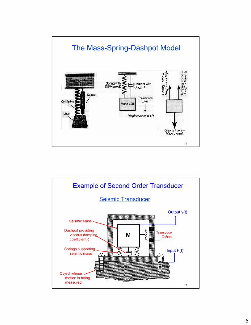
The Mass-Spring-Dashpot Model
12
Seismic Transducer
Transducer Output
Dashpot providing viscous damping coefficient ζ
Springs supporting seismic mass
Object whose motion is being measured
Seismic Mass
M
Input F(t)
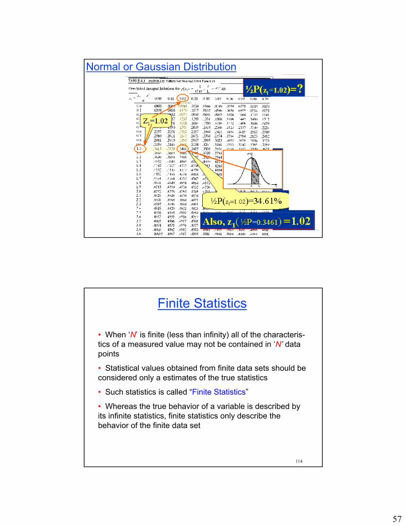
Output y(t)
Example of Second Order Transducer
7
13
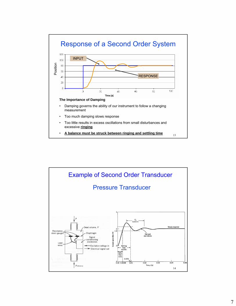
Response of a Second Order System
INPUT
RESPONSEPos
ition
The Importance of Damping
• Damping governs the ability of our instrument to follow a changing measurement
• Too much damping slows response
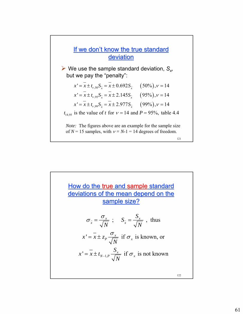
• Too little results in excess oscillations from small disturbances and excessive ringing
• A balance must be struck between ringing and settling time
14
Example of Second Order Transducer
Pressure Transducer
8
15
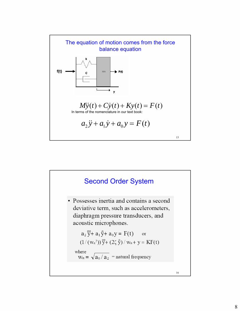
2 1 0 ( )a y a y a y F t+ + =&& &
f(t)
( ) ( ) ( ) ( )My t Cy t Ky t F t+ + =&& &
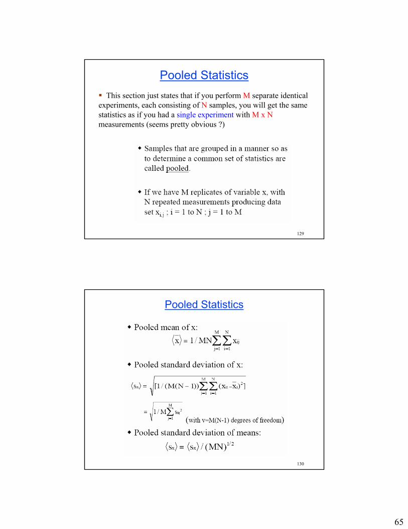
The equation of motion comes from the force balance equation
In terms of the nomenclature in our text book:
16
Second Order System
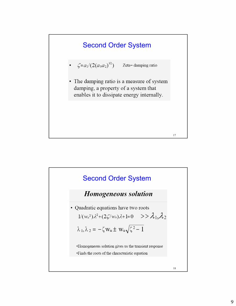
9
17
Second Order System
18
Second Order System
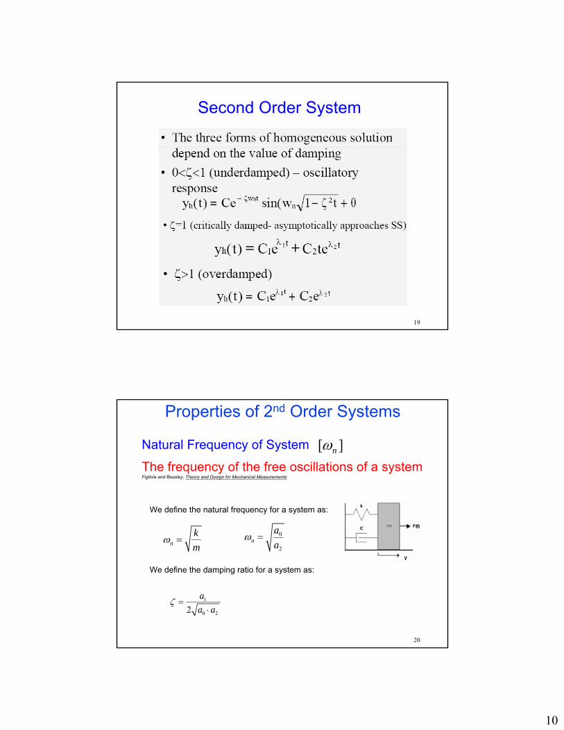
10
19
Second Order System
20
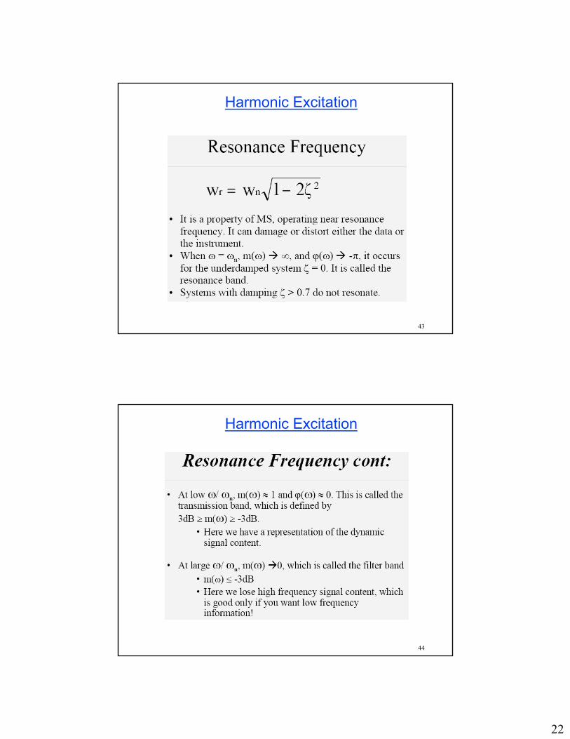
Properties of 2nd Order Systems
1
0 22aa a
ζ =⋅
0
2n
aa
ω =
[ ]nωNatural Frequency of System
The frequency of the free oscillations of a systemFigliola and Beasley, Theory and Design for Mechanical Measurements
We define the natural frequency for a system as:
nkm
ω =
We define the damping ratio for a system as:
11
21
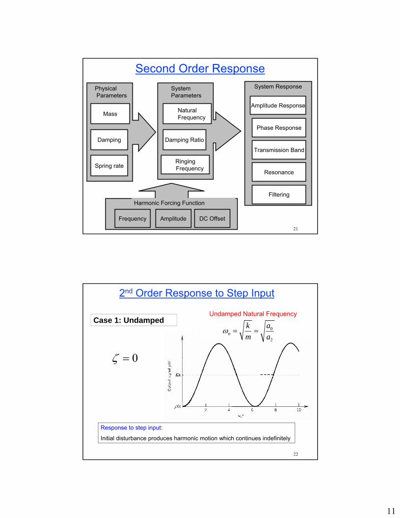
Second Order ResponsePhysicalParameters
Mass
Damping
Spring rate
System Parameters
Ringing Frequency
Natural Frequency
Damping Ratio
System Response
Amplitude Response
Phase Response
Resonance
Filtering
Transmission Band
Frequency Amplitude DC Offset
Harmonic Forcing Function
22
2nd Order Response to Step Input
0ζ =
Response to step input:
Initial disturbance produces harmonic motion which continues indefinitely
Case 1: UndampedUndamped Natural Frequency
0
2n
akm a
ω = =
12
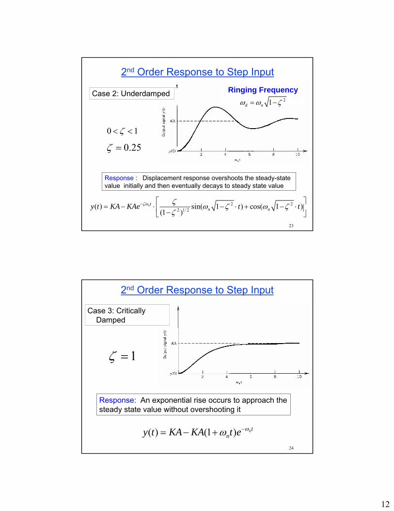
23
2nd Order Response to Step Input
0 1ζ< <
0.25ζ =
Response : Displacement response overshoots the steady-state value initially and then eventually decays to steady state value
2 22 1/ 2( ) sin( 1 ) cos( 1 )
(1 )nt
n ny t KA KAe t tζω ζ ω ζ ω ζζ
− ⎡ ⎤= − ⋅ − ⋅ + − ⋅⎢ ⎥−⎣ ⎦
Ringing Frequency21d nω ω ζ= −
Case 2: Underdamped
24
2nd Order Response to Step Input
1ζ =
Response: An exponential rise occurs to approach the steady state value without overshooting it
( ) (1 ) ntny t KA KA t e ωω −= − +
Case 3: Critically Damped
13
25
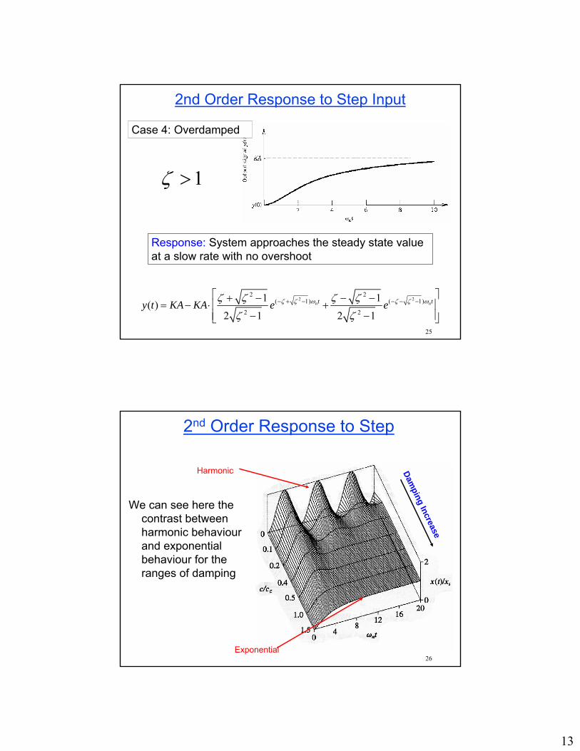
2nd Order Response to Step Input
1ζ >
Response: System approaches the steady state value at a slow rate with no overshoot
2 22 2
( 1) ( 1)
2 2
1 1( )
2 1 2 1n nt ty t KA KA e eζ ζ ω ζ ζ ωζ ζ ζ ζ
ζ ζ− + − − − −
⎡ ⎤+ − − −= − ⋅ +⎢ ⎥
⎢ ⎥− −⎣ ⎦
Case 4: Overdamped
26
2nd Order Response to Step
We can see here the contrast between harmonic behaviour and exponential behaviour for the ranges of damping
Harmonic
Exponential
Damping Increase
14
27
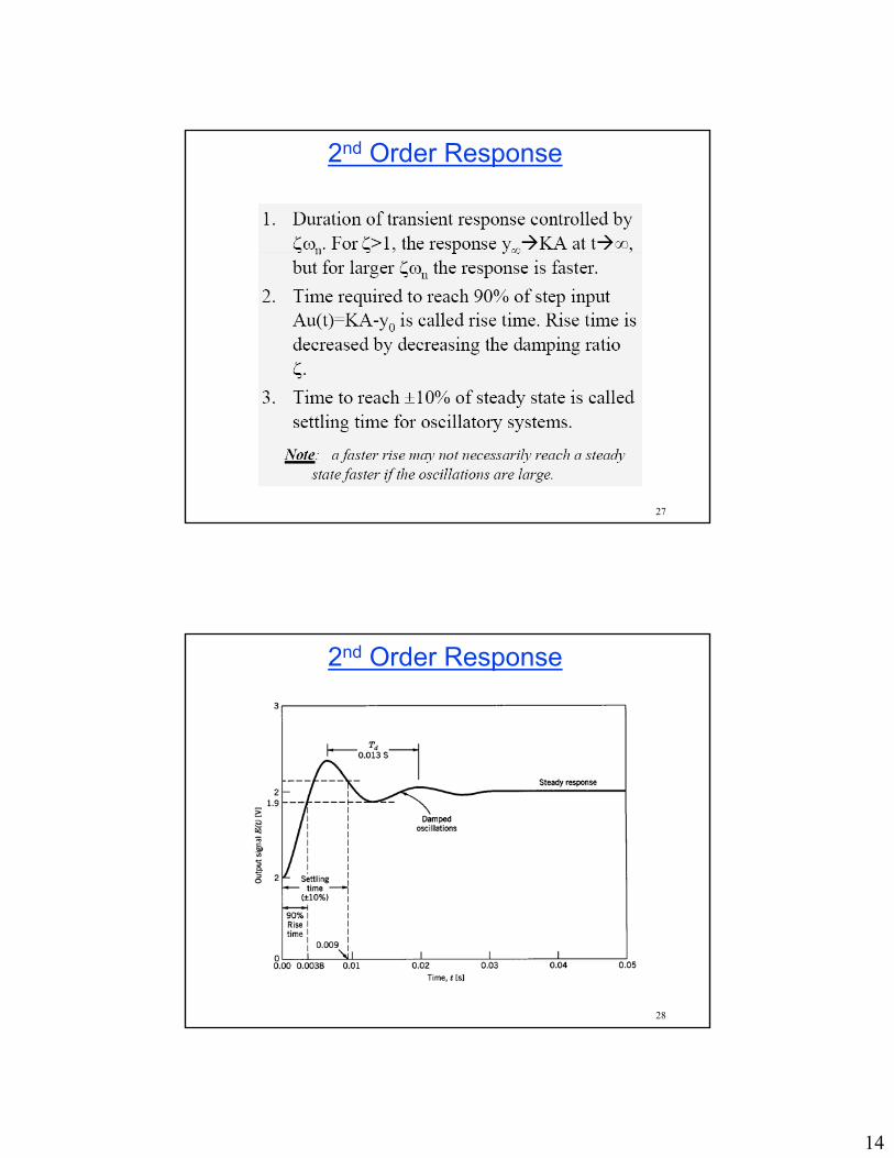
2nd Order Response
28
2nd Order Response
15
29
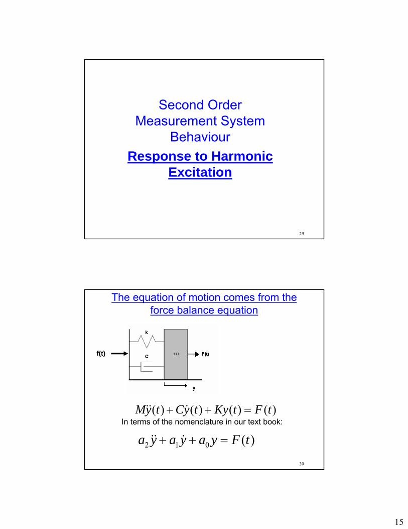
Second Order Measurement System
BehaviourResponse to Harmonic
Excitation
30
2 1 0 ( )a y a y a y F t+ + =&& &
f(t)
( ) ( ) ( ) ( )My t Cy t Ky t F t+ + =&& &
The equation of motion comes from the force balance equation
In terms of the nomenclature in our text book:
16
31
Natural Frequency of System
Defn: The frequency of the free oscillations of a system.
Figliola and Besley, Theory and Design for Mechanical Measurements
0
2n
aa
ω =
[ ]nω
We define the natural frequency for a system as:
nkm
ω =
EXPERIMENT: To find natural frequency of an undamped spring mass system, allowed to oscillate:
1. Set the system to vibrate naturally
2.n
cyclestime
ω =
32
Damping Ratio of System
Defn: A measure of system damping – a measure of a system’s ability to absorb or dissipate energy.
Figliola and Beasley, Theory and Design for Mechanical Measurements
1
0 22aa a
ζ =⋅
[ ]ζ
We define the damping ratio for a system as:
17
33
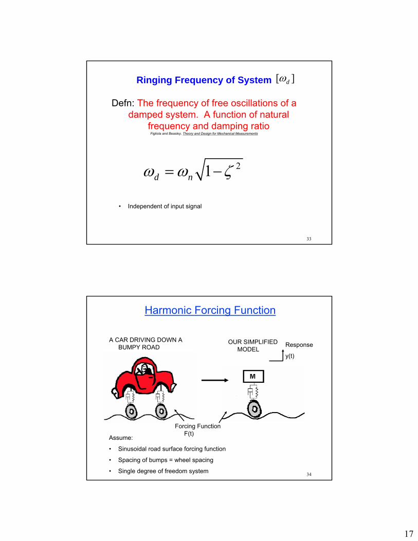
Ringing Frequency of System
Defn: The frequency of free oscillations of a damped system. A function of natural
frequency and damping ratioFigliola and Beasley, Theory and Design for Mechanical Measurements
[ ]dω
21d nω ω ζ= −
• Independent of input signal
34
Harmonic Forcing Function
OUR SIMPLIFIED MODEL
A CAR DRIVING DOWN A BUMPY ROAD
Assume:
• Sinusoidal road surface forcing function
• Spacing of bumps = wheel spacing
• Single degree of freedom system
Forcing Function F(t)
Response
y(t)
18
35
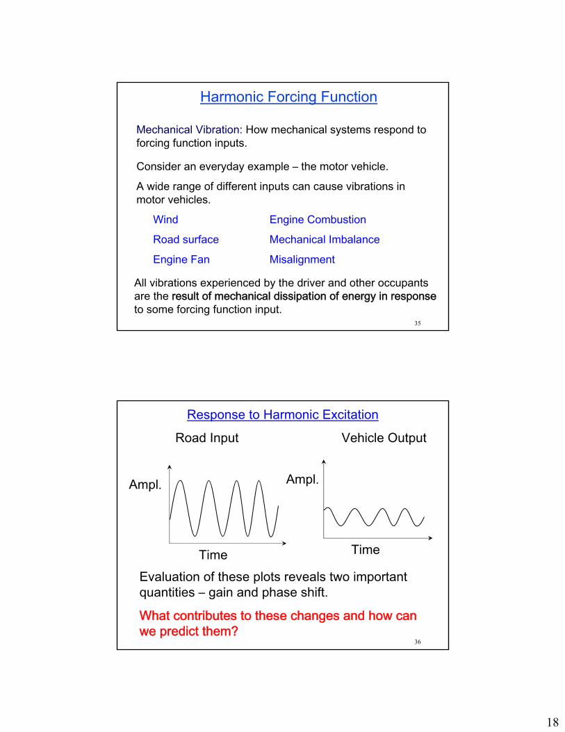
Mechanical Vibration: How mechanical systems respond to forcing function inputs.
Consider an everyday example – the motor vehicle.
A wide range of different inputs can cause vibrations in motor vehicles.
Wind Engine Combustion
Road surface Mechanical Imbalance
Engine Fan Misalignment
All vibrations experienced by the driver and other occupants are the result of mechanical dissipation of energy in responseto some forcing function input.
Harmonic Forcing Function
36
Road Input Vehicle Output
Response to Harmonic Excitation
Ampl.
Time
Ampl.
TimeEvaluation of these plots reveals two important quantities – gain and phase shift.
What contributes to these changes and how can we predict them?
19
37
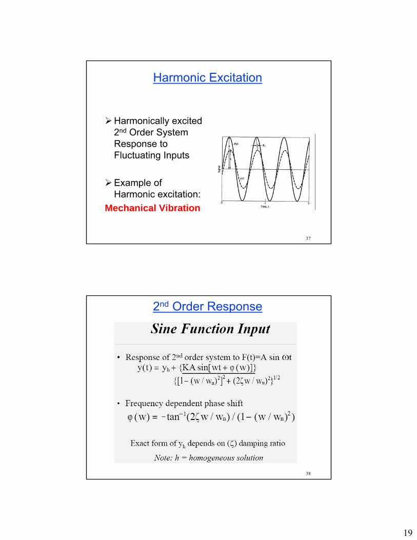
Harmonic Excitation
Harmonically excited 2nd Order System Response to Fluctuating Inputs
Example of Harmonic excitation:
Mechanical Vibration
38
2nd Order Response
20
39
Harmonic Excitation
40
Harmonic Excitation
21
41
Harmonic Excitation
42
Magnitude Ratio
OBSERVATIONS
• For low damping values, the amplitude is almost constant up to a frequency ratio of about 0.3
• For large damping values (overdamped case), the amplitude is reduced substantially
• More on p 94 of Figliola
Good linearity before frequency ratio of 0.3
22
43
Harmonic Excitation
44
Harmonic Excitation
23
45
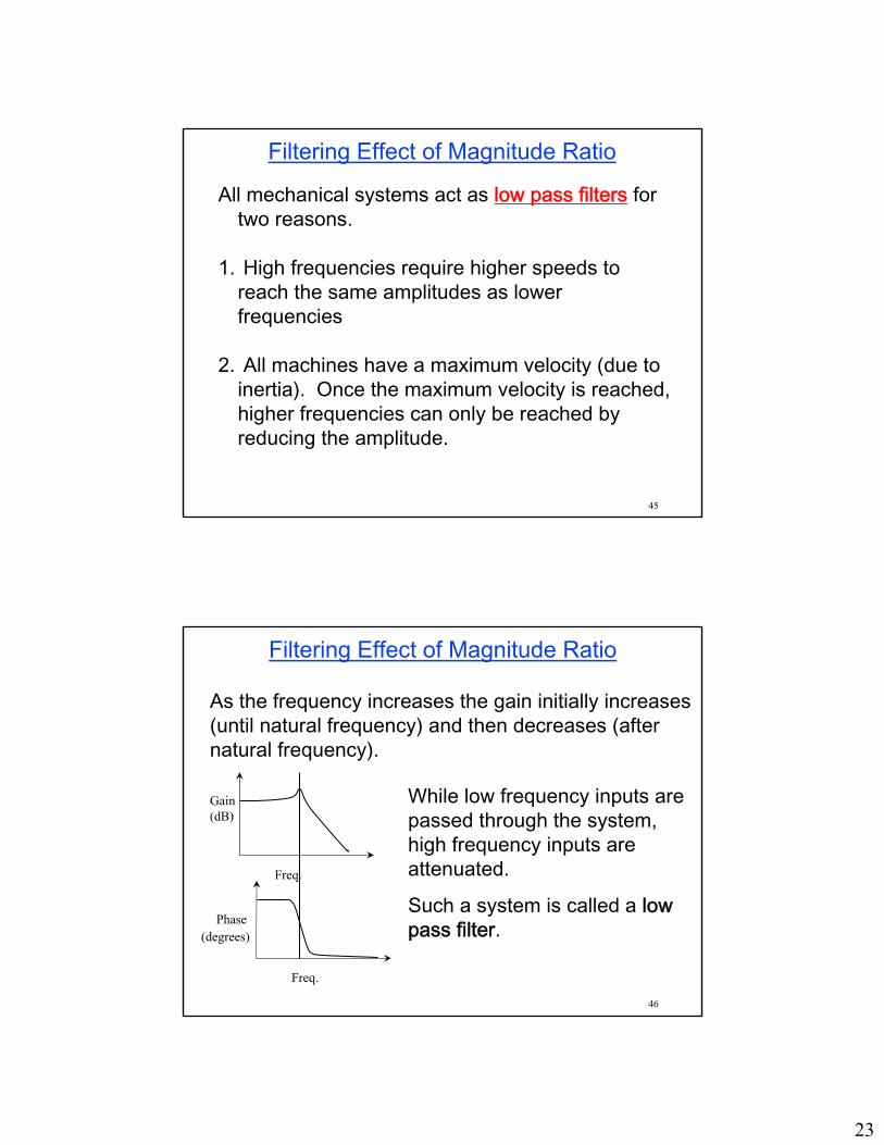
All mechanical systems act as low pass filters for two reasons.
1. High frequencies require higher speeds to reach the same amplitudes as lower frequencies
2. All machines have a maximum velocity (due to inertia). Once the maximum velocity is reached, higher frequencies can only be reached by reducing the amplitude.
Filtering Effect of Magnitude Ratio
46
As the frequency increases the gain initially increases (until natural frequency) and then decreases (after natural frequency).
While low frequency inputs are passed through the system, high frequency inputs are attenuated.
Such a system is called a low pass filter.
Gain(dB)
Freq.
Phase(degrees)
Freq.
Filtering Effect of Magnitude Ratio
24
47
OBSERVATIONS
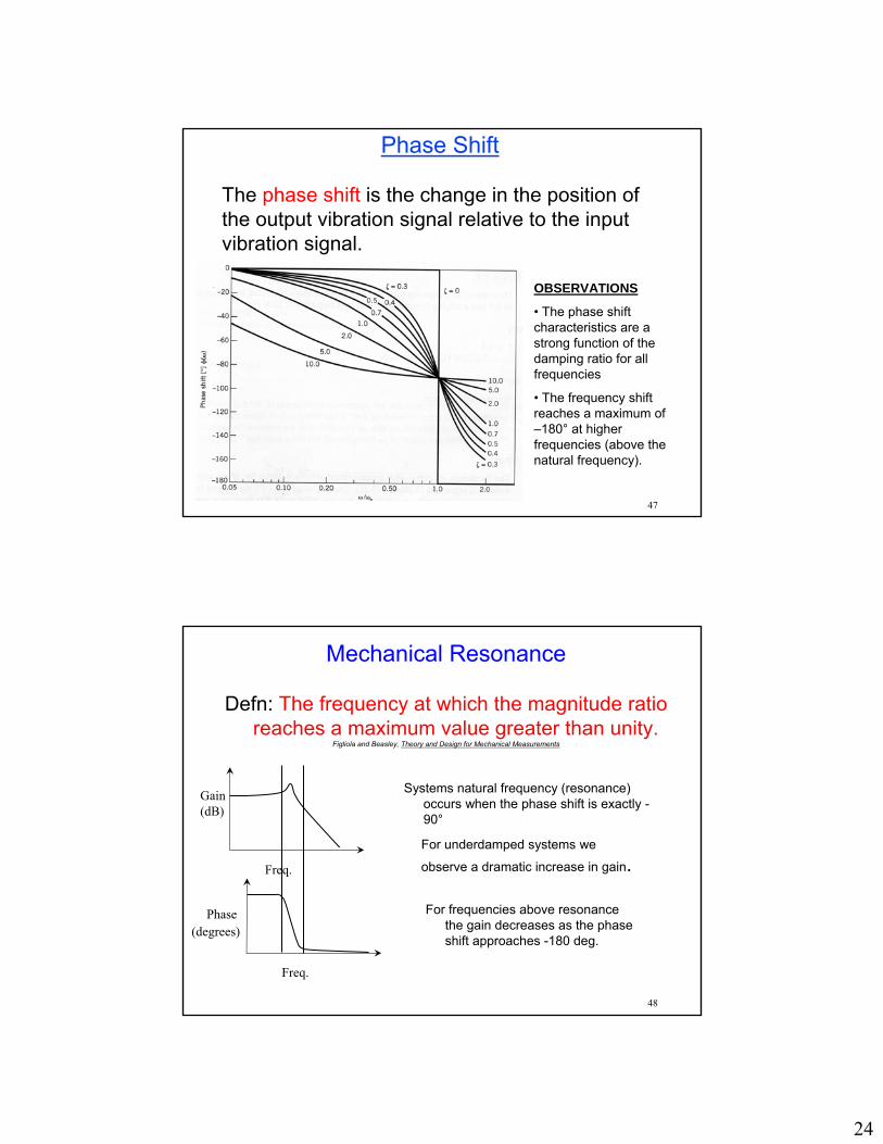
• The phase shift characteristics are a strong function of the damping ratio for all frequencies
• The frequency shift reaches a maximum of –180° at higher frequencies (above the natural frequency).
The phase shift is the change in the position of the output vibration signal relative to the input vibration signal.
Phase Shift
48
For underdamped systems we
observe a dramatic increase in gain.
Gain(dB)
Freq.
Phase(degrees)
Freq.
Mechanical Resonance
Defn: The frequency at which the magnitude ratio reaches a maximum value greater than unity.
Figliola and Beasley, Theory and Design for Mechanical Measurements
Systems natural frequency (resonance) occurs when the phase shift is exactly -90°
For frequencies above resonance the gain decreases as the phase shift approaches -180 deg.

25
49
Tacoma Narrows Bridge
The old Tacoma Narrows bridge was named Galloping Gertie after its completion in July 1940 because it vibrated violently in some wind conditionsCrossing it was like a roller-coaster ride, and Gertie was quite popular. November 7, 1940, a day high winds, Gertietook on a 30-hertz transverse vibration with an amplitude of 1½ feet!
50
Galloping Gertie After The Storm
• Wind-tunnel testing of bridge designs along with considerations for resonant behavior are now used to insure against similar disasters.
Old Tacoma Narrows Bridge New Narrows Bridge!
26
51
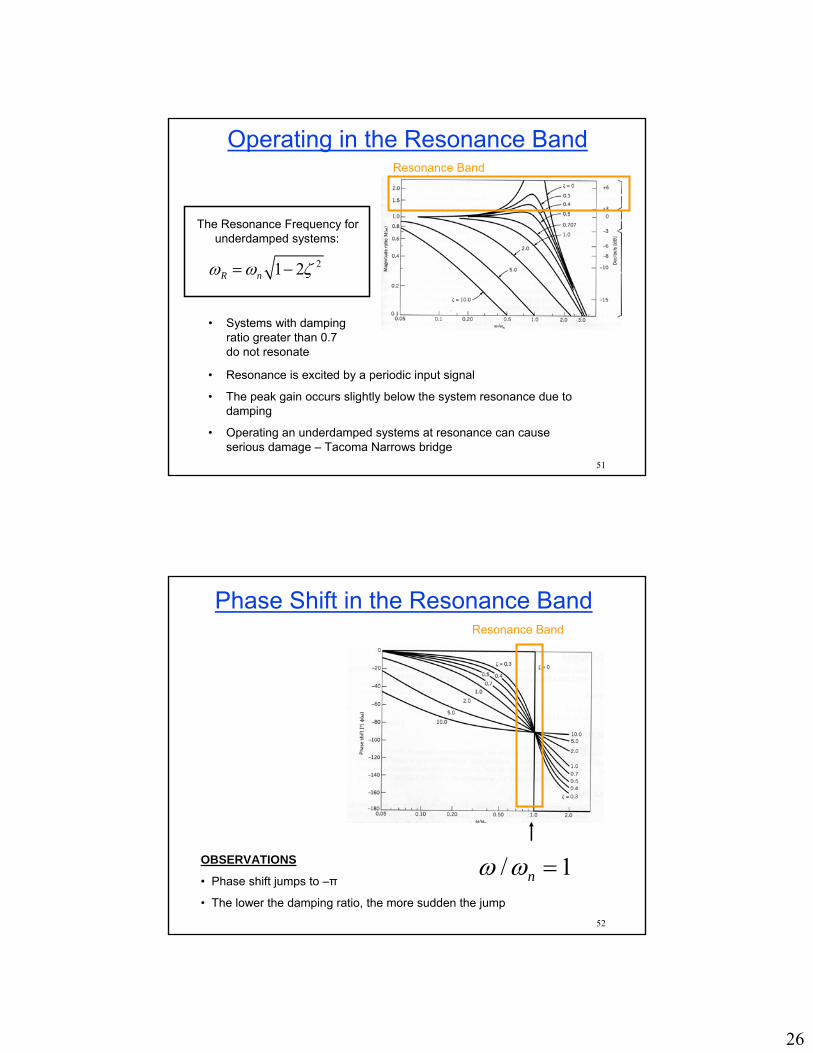
Operating in the Resonance Band
21 2R nω ω ζ= −
The Resonance Frequency for underdamped systems:
Resonance Band
• Resonance is excited by a periodic input signal
• The peak gain occurs slightly below the system resonance due to damping
• Operating an underdamped systems at resonance can cause serious damage – Tacoma Narrows bridge
• Systems with damping ratio greater than 0.7 do not resonate
52
Phase Shift in the Resonance Band
OBSERVATIONS
• Phase shift jumps to –π
• The lower the damping ratio, the more sudden the jump
Resonance Band
/ 1nω ω =
27
53
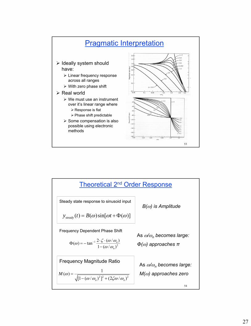
Pragmatic Interpretation
Ideally system should have:
Linear frequency response across all rangesWith zero phase shift
Real world We must use an instrument over it’s linear range where
Response is flatPhase shift predictable
Some compensation is also possible using electronic methods
54
Theoretical 2nd Order Response
12
2 ( / )( ) tan1 ( / )
n
n
ζ ω ωωω ω
− ⋅ ⋅Φ = −
−
2 2 2
1( )[1 ( / ) ] (2 / )n n
M ωω ω ζω ω
=− +
Frequency Dependent Phase Shift
Frequency Magnitude Ratio
As ω/ωn becomes large:
Φ(ω) approaches π
As ω/ωn becomes large:
M(ω) approaches zero
( ) ( )sin[ ( )]steadyy t B tω ω ω= + Φ
B(ω) is AmplitudeSteady state response to sinusoid input
28
55
56
29
57
58
30
59
60

31
61
62
32
63
Probability And Probability And StatisticsStatistics
64
Probability And StatisticsProbability And Statistics
33
65
Probability And StatisticsProbability And Statistics
66
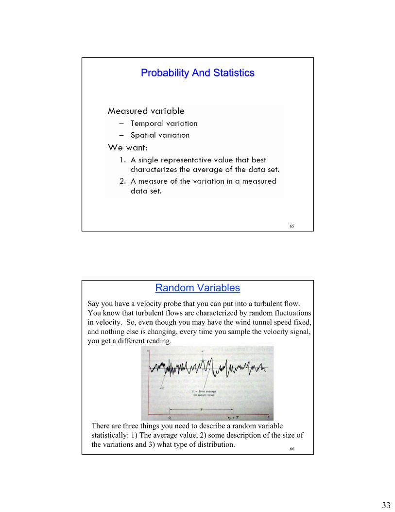
Random VariablesSay you have a velocity probe that you can put into a turbulent flow. You know that turbulent flows are characterized by random fluctuations in velocity. So, even though you may have the wind tunnel speed fixed, and nothing else is changing, every time you sample the velocity signal, you get a different reading.
There are three things you need to describe a random variable statistically: 1) The average value, 2) some description of the size of the variations and 3) what type of distribution.
34
67
Probability And StatisticsProbability And Statistics
We define x’ to be the true mean value of the random variable x. With a finite number of samples, we will never know the value of x’ exactly, but we will learn ways to estimate it.
68
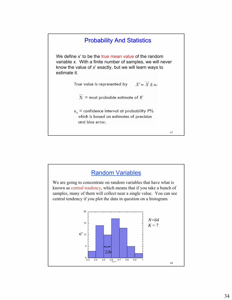
Random VariablesWe are going to concentrate on random variables that have what is known as central tendency, which means that if you take a bunch of samples, many of them will collect near a single value. You can see central tendency if you plot the data in question on a histogram.
0
5
10
15
20
0.3 0.4 0.5 0.6 0.7 0.8 0.9 1
Thermo II 2002
Cou
nt
out of 1
n j
N=64K = 7
}
2δx
35
69
Probability Density Function
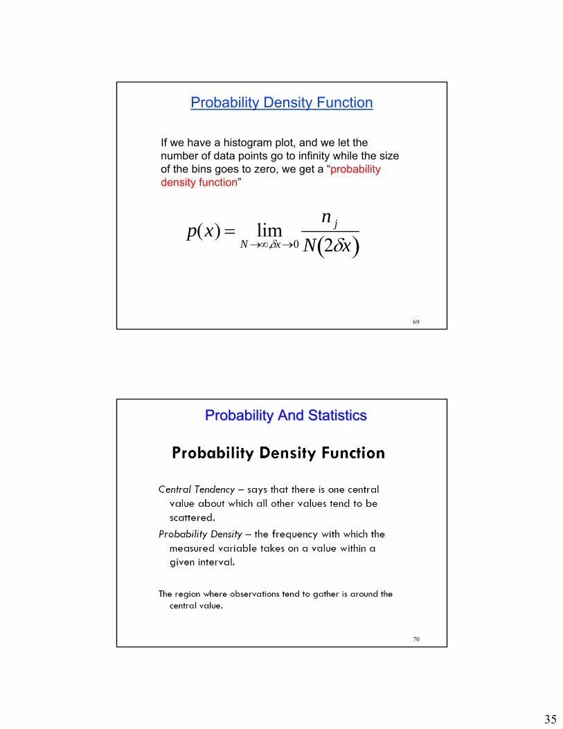
If we have a histogram plot, and we let the number of data points go to infinity while the size of the bins goes to zero, we get a “probability density function”
p(x) = limN →∞,δx →0
n j
N 2δx( )
70
Probability And StatisticsProbability And Statistics
36
71
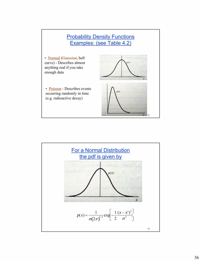
Probability Density FunctionsExamples: (see Table 4.2)
• Normal (Gaussian, bell curve) - Describes almost anything real if you take enough data
• Poisson - Describes events occurring randomly in time (e.g. radioactive decay)
72
For a Normal Distribution the pdf is given by
p(x) =1
σ 2π( )1/ 2 exp −12
(x − x ')2
σ 2
⎡
⎣ ⎢
⎤
⎦ ⎥
37
73
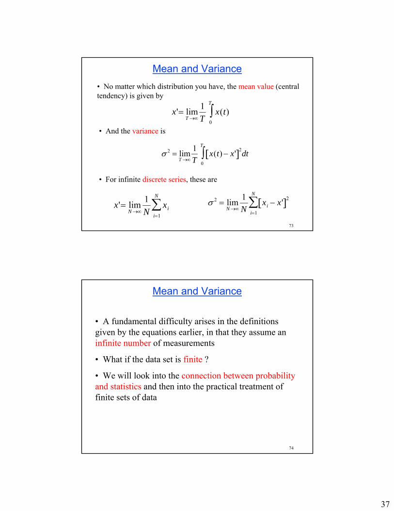
Mean and Variance• No matter which distribution you have, the mean value (central tendency) is given by
x'= limT →∞
1T
x(t)0
T
∫• And the variance is
σ 2 = limT →∞
1T
x(t) − x'[ ]2
0
T
∫ dt
• For infinite discrete series, these are
x'= limN →∞
1N
xii=1
N
∑ σ 2 = limN →∞
1N
xi − x '[ ]2
i=1
N
∑
74
Mean and Variance
• A fundamental difficulty arises in the definitions given by the equations earlier, in that they assume an infinite number of measurements
• What if the data set is finite ?
• We will look into the connection between probability and statistics and then into the practical treatment of finite sets of data
38
75
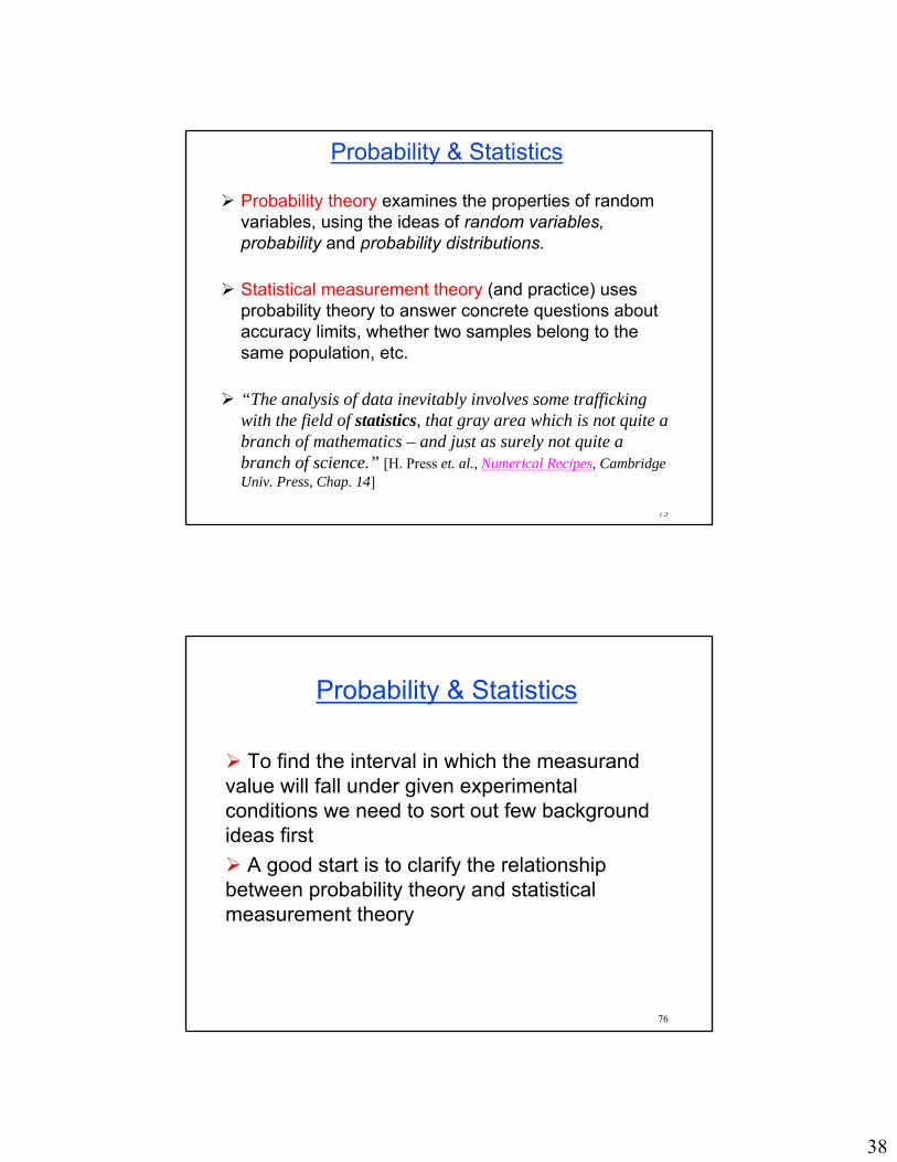
Probability theory examines the properties of random variables, using the ideas of random variables, probability and probability distributions.
Statistical measurement theory (and practice) uses probability theory to answer concrete questions about accuracy limits, whether two samples belong to the same population, etc.
“The analysis of data inevitably involves some trafficking with the field of statistics, that gray area which is not quite a branch of mathematics – and just as surely not quite a branch of science.” [H. Press et. al., Numerical Recipes, Cambridge Univ. Press, Chap. 14]
Probability & Statistics
76
Probability & Statistics
To find the interval in which the measurandvalue will fall under given experimental conditions we need to sort out few background ideas first
A good start is to clarify the relationship between probability theory and statistical measurement theory
39
77
Probability And StatisticsProbability And Statistics
78
See Example 4.1 page 112
Probability And StatisticsProbability And Statistics

40
79
Having a set of repeated measurement Having a set of repeated measurement data, we want to know how to:data, we want to know how to:
1. Find the best estimate for the measured variable (the measurand)
2. Find the best estimate for the measurandvariability
3. Find the interval in which the measurandvalue will fall under given experimental conditions
80
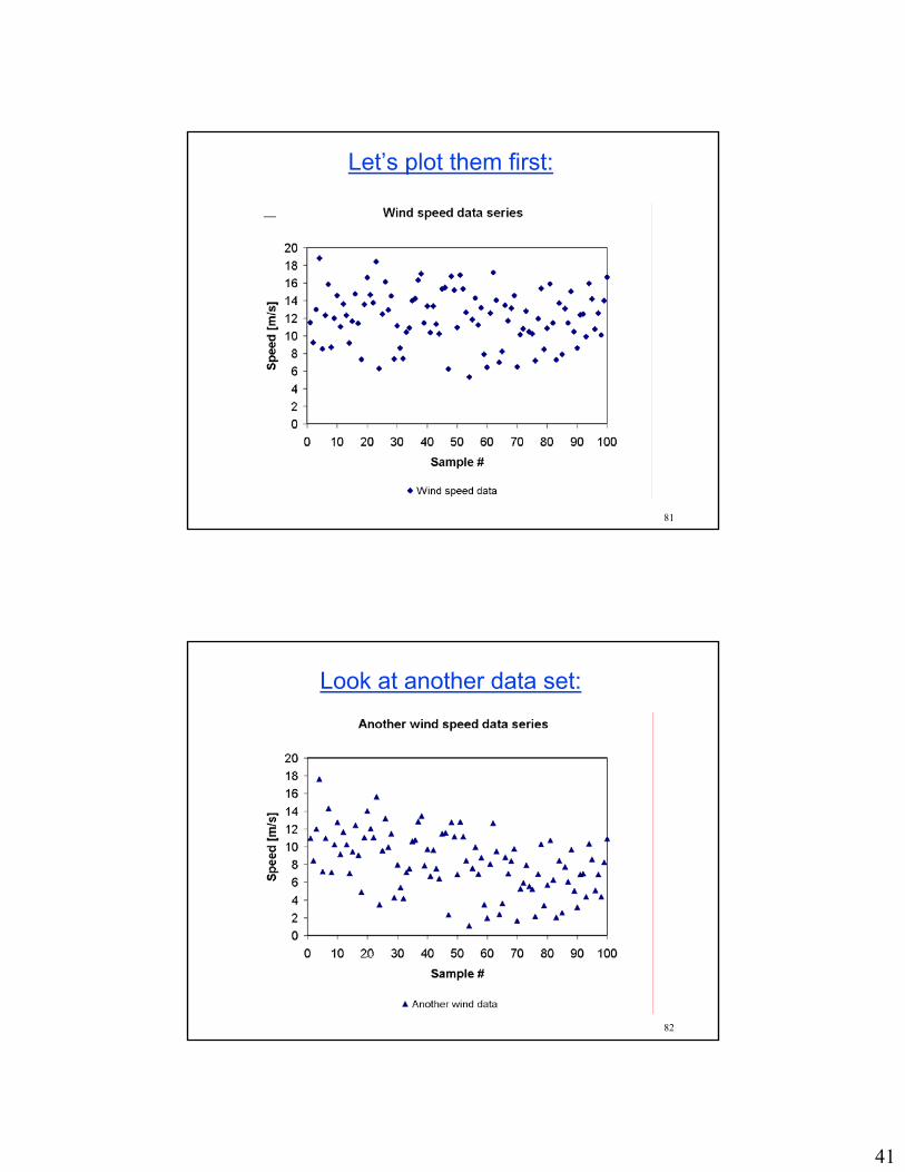
Example: Consider the Wind speed data:
Sample #Wind
speed data
Running average Sample #
Wind speed data
Running average Sample #
Wind speed data
Running average Sample #
Wind speed data
Running average
1 11.5365 11.5365 26 16.1416 12.6104 51 16.9181 12.5474 76 7.1871 12.08292 9.2332 10.3849 27 12.9392 12.6226 52 15.3221 12.6008 77 11.9689 12.08143 12.9846 11.2515 28 14.5035 12.6898 53 12.6510 12.6017 78 15.3700 12.12364 18.7957 13.1375 29 7.3669 12.5062 54 5.3269 12.4670 79 8.4892 12.07765 8.5051 12.2110 30 11.1278 12.4603 55 11.8757 12.4563 80 10.8533 12.06236 12.3544 12.2349 31 8.6197 12.3364 56 14.2836 12.4889 81 15.8850 12.10957 15.8414 12.7501 32 7.4469 12.1836 57 11.2585 12.4673 82 11.4947 12.10208 8.7258 12.2471 33 10.4165 12.1300 58 13.1818 12.4796 83 7.3016 12.04419 11.9886 12.2184 34 10.9251 12.0946 59 7.8915 12.4019 84 13.7059 12.0639
10 14.5874 12.4553 35 14.0136 12.1494 60 6.4132 12.3020 85 7.8833 12.014711 11.0471 12.3272 36 14.2179 12.2069 61 12.5804 12.3066 86 13.0810 12.027112 13.6365 12.4363 37 16.3352 12.3185 62 17.2129 12.3857 87 11.4623 12.020613 12.3296 12.4281 38 17.0296 12.4424 63 14.0680 12.4124 88 15.0626 12.055214 9.1848 12.1965 39 11.4896 12.4180 64 7.0001 12.3279 89 10.4630 12.037315 11.6655 12.1611 40 13.3769 12.4420 65 8.2330 12.2649 90 8.6416 11.999616 14.7416 12.3224 41 10.3996 12.3922 66 13.4989 12.2836 91 12.3941 12.003917 11.4189 12.2692 42 13.3815 12.4157 67 11.7140 12.2751 92 12.4995 12.009318 7.3487 11.9958 43 11.3415 12.3907 68 13.1620 12.2881 93 9.9212 11.986919 13.5740 12.0789 44 10.2202 12.3414 69 14.5516 12.3209 94 15.9513 12.029020 16.6338 12.3067 45 15.3365 12.4080 70 6.4819 12.2375 95 14.1887 12.051821 14.6856 12.4199 46 15.4909 12.4750 71 10.1296 12.2078 96 10.7504 12.038222 13.7430 12.4801 47 6.2576 12.3427 72 10.8048 12.1883 97 12.5755 12.043723 18.4066 12.7378 48 16.7661 12.4348 73 12.8268 12.1971 98 10.0896 12.023824 6.2973 12.4694 49 15.1833 12.4909 74 10.4948 12.1741 99 14.0007 12.043825 12.4632 12.4692 50 10.9444 12.4600 75 10.2319 12.1482 100 16.6868 12.0902
41
81
Let’s plot them first:
82
Look at another data set:
42
83
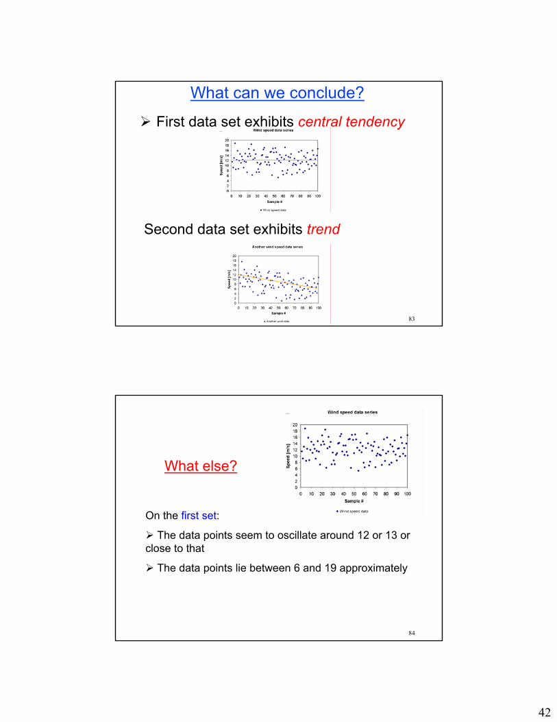
What can we conclude?
First data set exhibits central tendency
Second data set exhibits trend
84
What else?
On the first set:
The data points seem to oscillate around 12 or 13 or close to that
The data points lie between 6 and 19 approximately

43
85
Next, we can make a histogram
Histogram
0
10
20
30
40
50
60
6 10 14 18 MoreB in
Histogram
0
5
10
15
20
25
30
6 8 10 12 14 16 18
Mor
e
B in
Histogram
02468
10121416
6 7 8 9 10 11 12 13 14 15 16 17 18
Mor
e
Bin
Freq
uenc
y
Which one is the right one?
Number of bins, K = 1.87(N-1)0.4 + 1 (Eq. 4.2) pg. 111
For our data, N = 100, K = 13
86
Next, we can make a histogram
Histogram
0
10
20
30
40
50
60
6 10 14 18 MoreB in
Histogram
0
5
10
15
20
25
30
6 8 10 12 14 16 18
Mor
e
B in
Histogram
02468
10121416
6 7 8 9 10 11 12 13 14 15 16 17 18
Mor
e
Bin
Freq
uenc
y
Which one is the right one?
Number of bins, K = 1.87(N-1)0.4 + 1 (Eq. 4.2) pg. 111
For our data, N = 100, K = 13
44
87
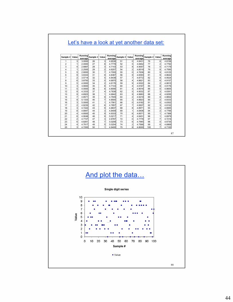
Let’s have a look at yet another data set:
Sample # Value Running average Sample # Value Running
average Sample # Value Running average Sample # Value Running
average1 3 3.0000 26 3 4.6538 51 0 4.8431 76 6 4.81582 1 2.0000 27 8 4.7778 52 5 4.8462 77 2 4.77923 4 2.6667 28 3 4.7143 53 8 4.9057 78 0 4.71794 1 2.2500 29 2 4.6207 54 2 4.8519 79 8 4.75955 5 2.8000 30 7 4.7000 55 0 4.7636 80 9 4.81256 9 3.8333 31 9 4.8387 56 9 4.8393 81 9 4.86427 2 3.5714 32 5 4.8438 57 7 4.8772 82 8 4.90248 6 3.8750 33 0 4.6970 58 4 4.8621 83 6 4.91579 5 4.0000 34 2 4.6176 59 9 4.9322 84 2 4.881010 3 3.9000 35 8 4.7143 60 4 4.9167 85 8 4.917611 5 4.0000 36 8 4.8056 61 4 4.9016 86 0 4.860512 8 4.3333 37 4 4.7838 62 5 4.9032 87 3 4.839113 9 4.6923 38 1 4.6842 63 9 4.9683 88 4 4.829514 7 4.8571 39 9 4.7949 64 2 4.9219 89 8 4.865215 9 5.1333 40 7 4.8500 65 3 4.8923 90 2 4.833316 3 5.0000 41 1 4.7561 66 0 4.8182 91 5 4.835217 2 4.8235 42 6 4.7857 67 7 4.8507 92 3 4.815218 3 4.7222 43 9 4.8837 68 8 4.8971 93 4 4.806519 8 4.8947 44 3 4.8409 69 1 4.8406 94 2 4.776620 4 4.8500 45 9 4.9333 70 6 4.8571 95 1 4.736821 6 4.9048 46 9 5.0217 71 4 4.8451 96 1 4.697922 2 4.7727 47 3 4.9787 72 0 4.7778 97 7 4.721623 6 4.8261 48 7 5.0208 73 6 4.7945 98 0 4.673524 4 4.7917 49 5 5.0204 74 2 4.7568 99 6 4.686925 3 4.7200 50 1 4.9400 75 8 4.8000 100 7 4.7100
88
And plot the data…
45
89
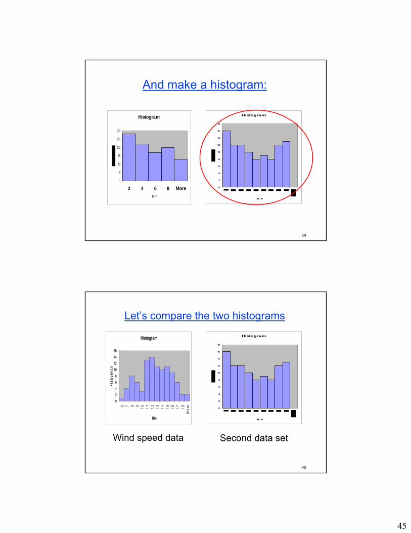
And make a histogram:
Histogram
0
5
10
15
20
25
30
2 4 6 8 MoreBin
Histogram
0
2
4
6
8
10
12
14
16
18
Bin
90
Let’s compare the two histograms
Histogram
02468
10121416
6 7 8 9 10 11 12 13 14 15 16 17 18M
ore
Bin
Freq
uenc
y
Histogram
0
2
4
6
8
10
12
14
16
18
Bin
Wind speed data Second data set
46
91
Answer to Question 1:
1. To find the best estimate for the measured variable (the measurand)
Use the mean value!
1
1 N
ix xN
= ∑
92
Answer to Question 2:
2. To find the best estimate for the measurand variability
Use the Sample variance
Or the Sample standard deviation
( )2
2
1
11
N
x iS x xN
= −− ∑
2x xS S=
47
93
How do we add up sample means, How do we add up sample means, variances and standard deviations?variances and standard deviations?
Let x a b= + Then,
2 2 2
2 2
x a b
x a b
x a bS S S
S S S
= +
= +
= +
Means add up
Standard deviations don’t simplyadd up
Variances add up
Provided that a and b are uncorrelated!
94
A bathroom scale example
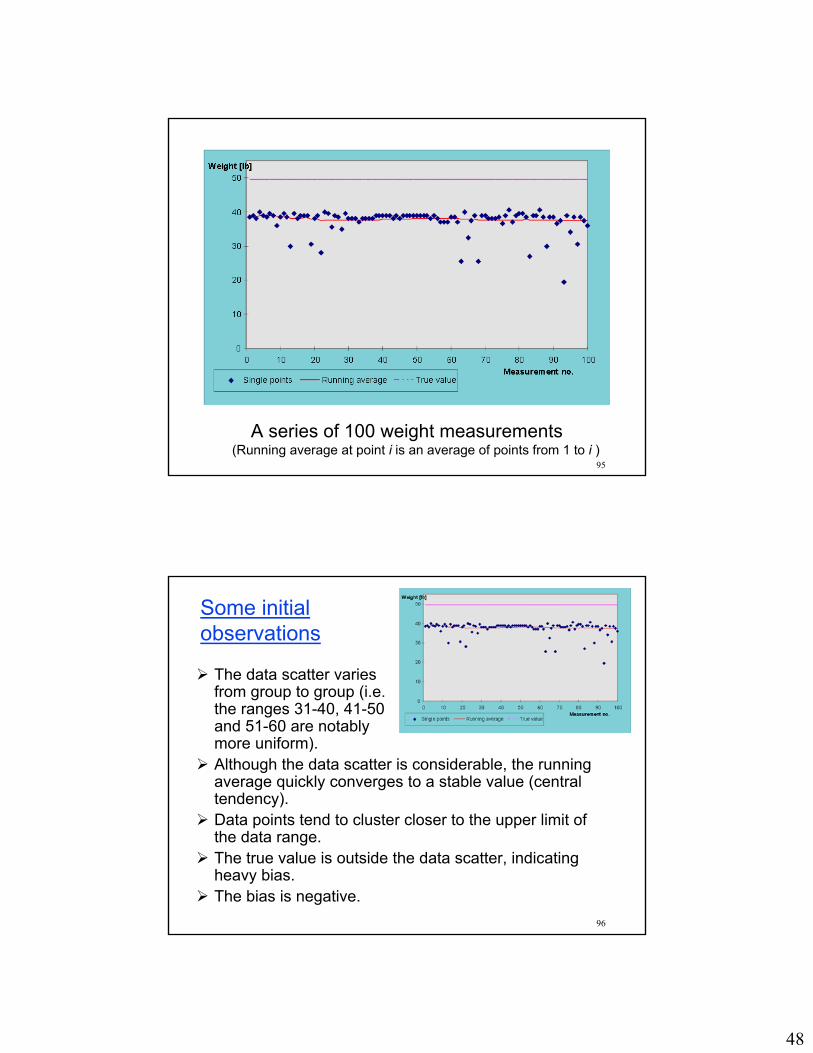
A series of 100 weight measurements were performed on a (badly tuned) bathroom scale. A weight of 50 lb was repeatedly measured by a class in 1996.10 groups made 10 measurements each.
The raw data with running average is shown in the following figure.
48
95
A series of 100 weight measurements(Running average at point i is an average of points from 1 to i )
96
Some initial observations
The data scatter varies from group to group (i.e. the ranges 31-40, 41-50 and 51-60 are notably more uniform).Although the data scatter is considerable, the running average quickly converges to a stable value (central tendency).Data points tend to cluster closer to the upper limit of the data range.The true value is outside the data scatter, indicating heavy bias.The bias is negative.
49
97
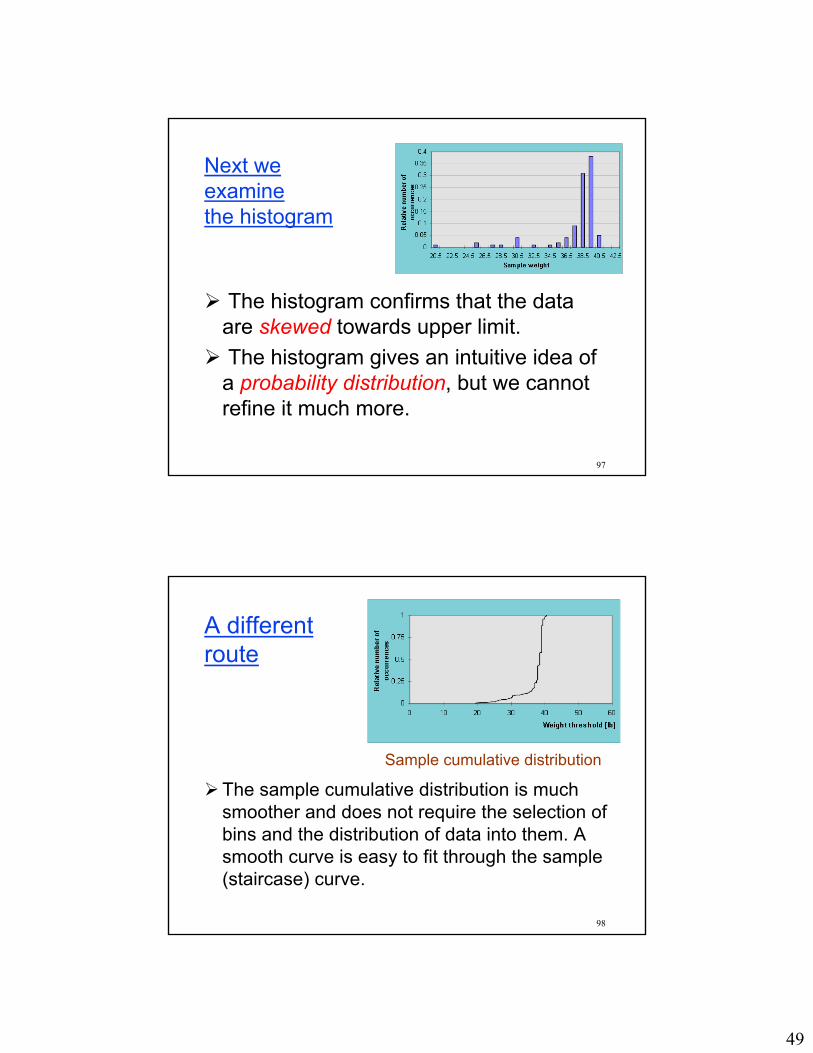
Next we examinethe histogram
The histogram confirms that the data are skewed towards upper limit. The histogram gives an intuitive idea of a probability distribution, but we cannot refine it much more.
98
A different route
The sample cumulative distribution is much smoother and does not require the selection of bins and the distribution of data into them. A smooth curve is easy to fit through the sample (staircase) curve.
Sample cumulative distribution
50
99
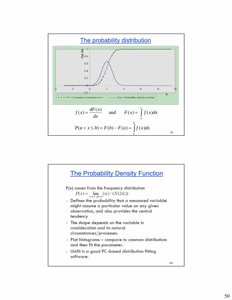
The probability distribution
( )( ) and ( ) ( )
( ) ( ) ( ) ( )
x
b
a
dF xf x F x f x dxdx
P a x b F b F a f x dx
−∞
= =
< ≤ = − =
∫
∫
100
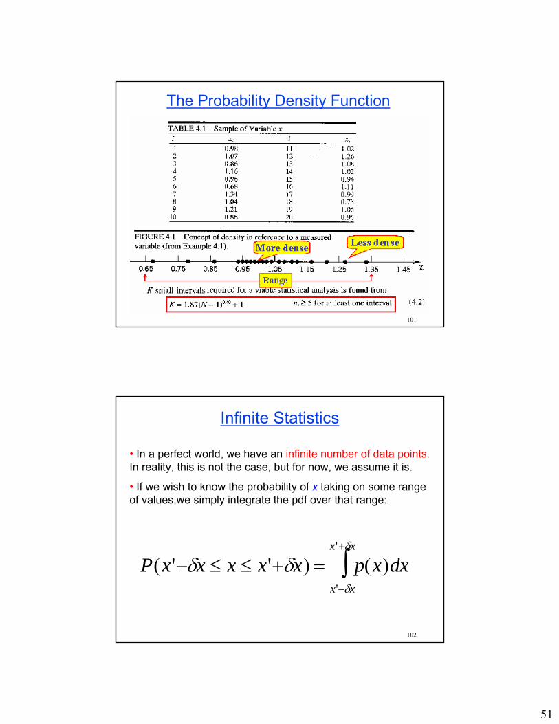
The Probability Density Function
51
101
The Probability Density Function
102
Infinite Statistics
• In a perfect world, we have an infinite number of data points. In reality, this is not the case, but for now, we assume it is.
• If we wish to know the probability of x taking on some range of values,we simply integrate the pdf over that range:
P(x'−δx ≤ x ≤ x'+δx) = p(x)dxx'−δx
x'+δx
∫
52
103
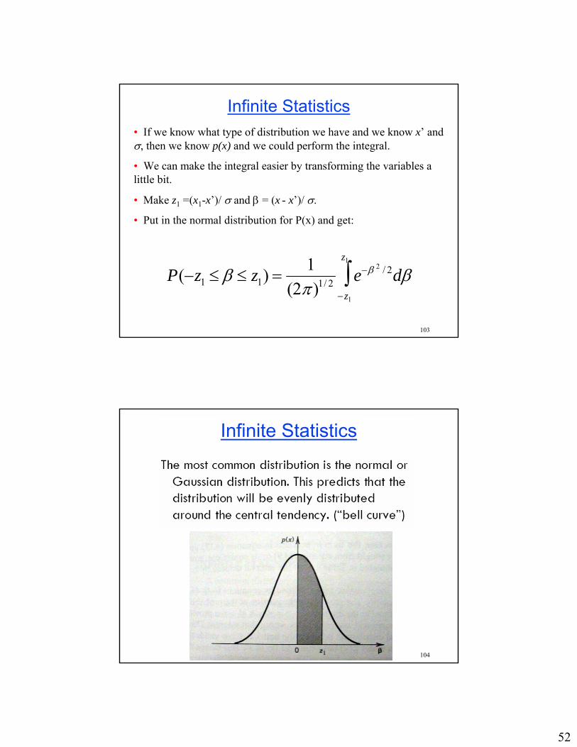
Infinite Statistics• If we know what type of distribution we have and we know x’ and σ, then we know p(x) and we could perform the integral.
• We can make the integral easier by transforming the variables a little bit.
• Make z1 =(x1-x’)/ σ and β = (x - x’)/ σ.
• Put in the normal distribution for P(x) and get:
P(−z1 ≤ β ≤ z1) =1
(2π )1/ 2 e−β 2 / 2
−z1
z1
∫ dβ
104
Infinite Statistics
53
105
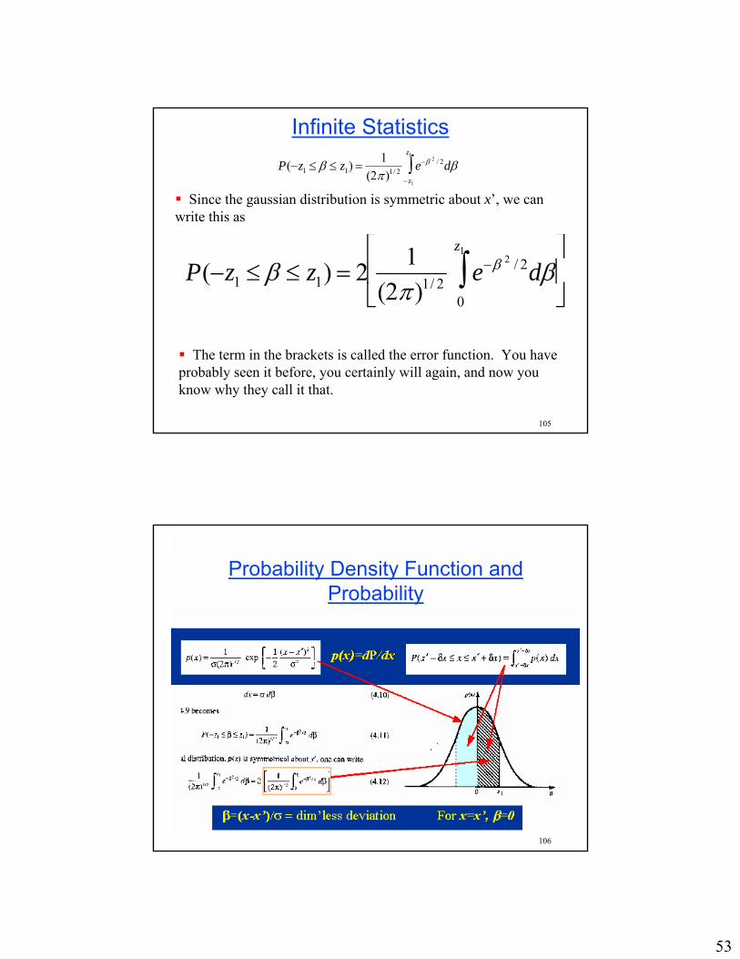
Infinite StatisticsP(−z1 ≤ β ≤ z1) =
1(2π )1/ 2 e−β 2 / 2
−z1
z1
∫ dβ
Since the gaussian distribution is symmetric about x’, we can write this as
P(−z1 ≤ β ≤ z1) = 2 1(2π )1/ 2 e−β 2 / 2
0
z1
∫ dβ⎡
⎣ ⎢
⎤
⎦ ⎥
The term in the brackets is called the error function. You have probably seen it before, you certainly will again, and now you know why they call it that.
106
Probability Density Function and Probability

54
107
Probability values for Normal Error FunctionsTable 4.2
108
Normal or Gaussian Distribution
z = 1 z = 2 z = 3z = 0z = –1z = –2z = –3
'x xzσ−
=
Note: p(x) is the “probability density of x”
See Table 4.2 pg,. See Table 4.2 pg,. 114 for other types 114 for other types of distributionsof distributions
P(−z1 ≤ β ≤ z1) =1
(2π )1/ 2 e−β 2 / 2
−z1
z1
∫ dβ
55
109
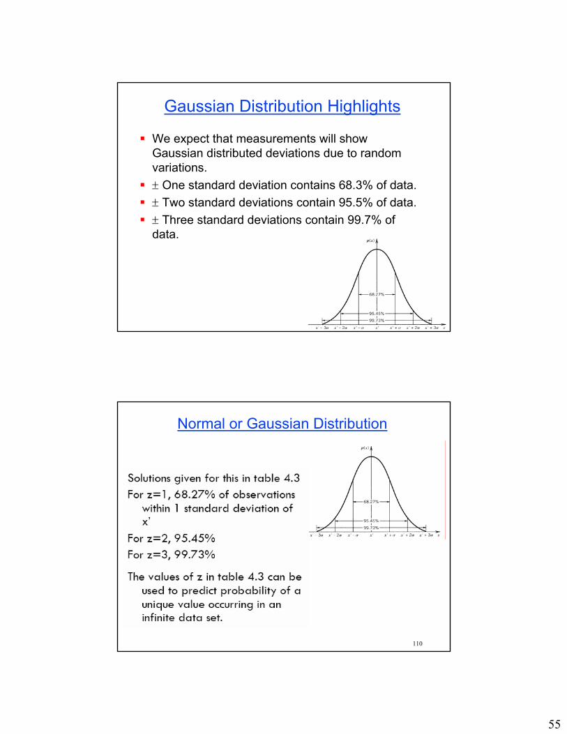
Gaussian Distribution Highlights
We expect that measurements will show Gaussian distributed deviations due to random variations.± One standard deviation contains 68.3% of data.± Two standard deviations contain 95.5% of data.± Three standard deviations contain 99.7% of data.
110
Normal or Gaussian Distribution
56
111
Normal or Gaussian Distribution
112
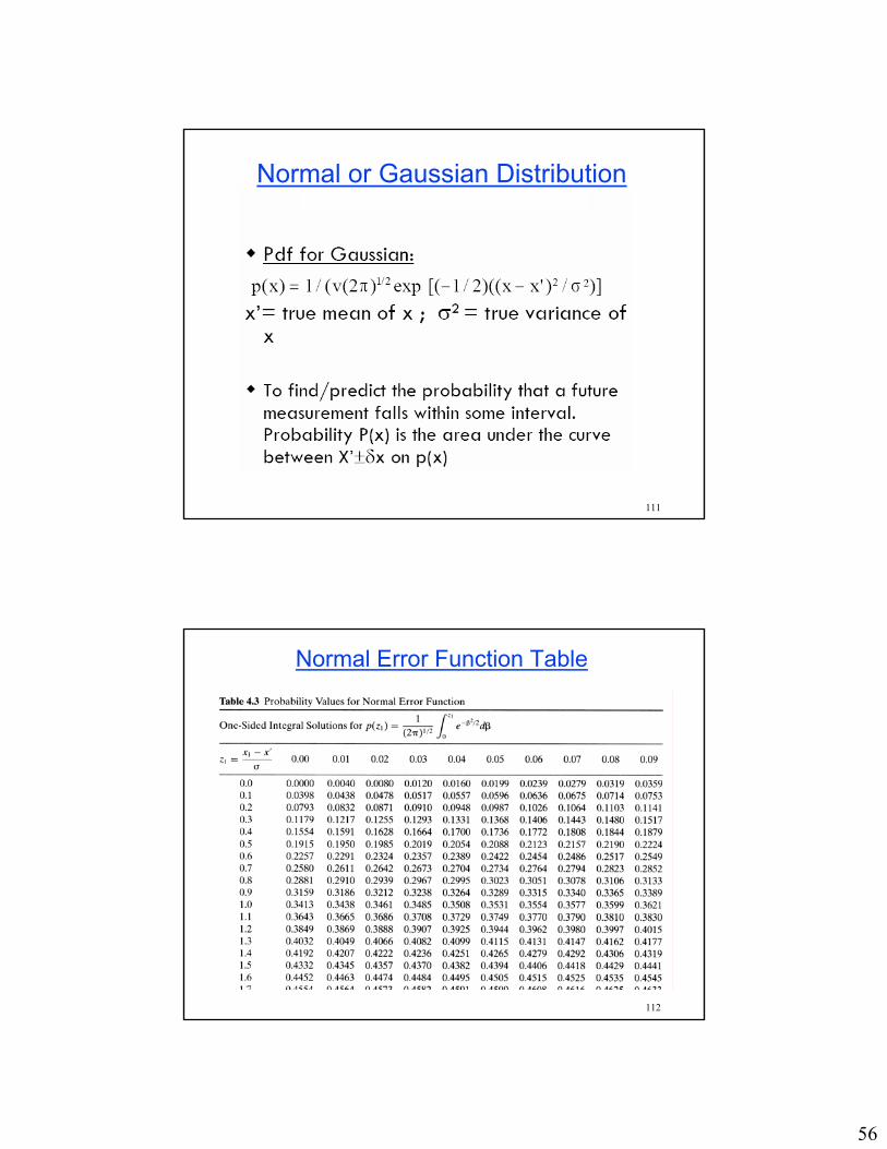
Normal Error Function Table
57
113
Normal or Gaussian Distribution
114
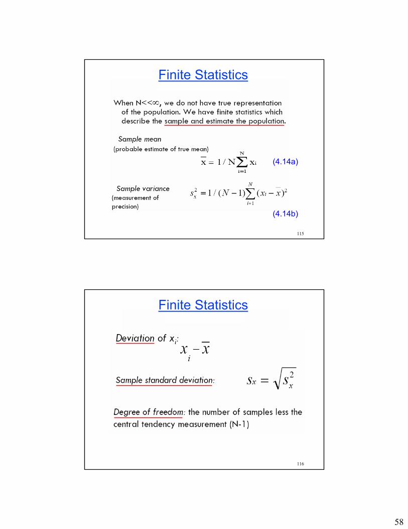
Finite Statistics
• When ‘N’ is finite (less than infinity) all of the characteris-tics of a measured value may not be contained in ‘N’ data points
• Statistical values obtained from finite data sets should be considered only a estimates of the true statistics
• Such statistics is called “Finite Statistics”
• Whereas the true behavior of a variable is described by its infinite statistics, finite statistics only describe the behavior of the finite data set
58
115
(4.14a)
(4.14b)
Finite Statistics
116
Finite Statistics
59
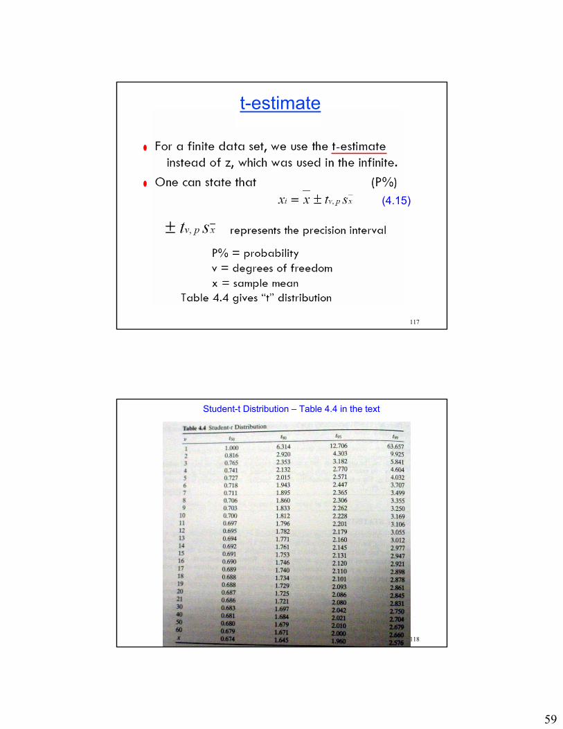
117
(4.15)
t-estimate
118
Student-t Distribution – Table 4.4 in the text
60
119
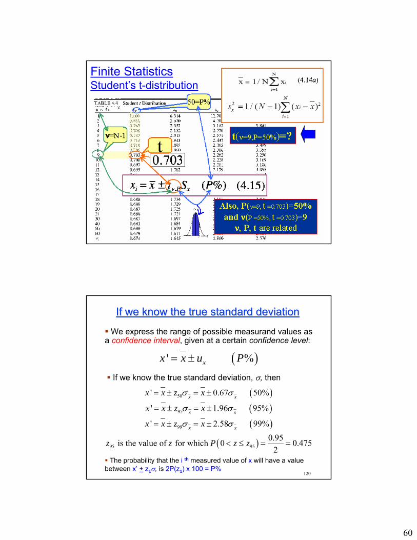
Finite StatisticsStudent’s t-distribution
120
If we know the true standard deviationIf we know the true standard deviation
We express the range of possible measurand values as a confidence interval, given at a certain confidence level:
( )' %xx x u P= ±
If we know the true standard deviation, σ, then
( )( )( )
( )
50
95
99
95 95
' 0.67 50%
' 1.96 95%
' 2.58 99%0.95 is the value of for which 0 0.475
2
x x
x x
x x
x x z x
x x z x
x x z x
z z P z z
σ σ
σ σ
σ σ
= ± = ±
= ± = ±
= ± = ±
< ≤ = =
The probability that the i th measured value of x will have a value between x’ + z1σ, is 2P(z1) x 100 = P%
61
121
If we donIf we don’’t know the true standard t know the true standard deviationdeviation
We use the sample standard deviation, Sx, but we pay the “penalty”:
( )( )( )
,50
,95
,99
14,95
' 0.692 50% , 14
' 2.145 95% , 14
' 2.977 99% , 14 is the value of for 14 and 95%, table 4.4
x x
x x
x x
x x t S x S
x x t S x S
x x t S x St t P
ν
ν
ν
ν
ν
νν
= ± = ± =
= ± = ± =
= ± = ± =
= =
Note: The figures above are an example for the sample sizeof N = 15 samples, with ν = N-1 = 14 degrees of freedom.
122
How do the How do the truetrue and and samplesample standard standard deviations of the mean depend on the deviations of the mean depend on the
sample size?sample size?
1,
; , thus
' if is known, or
' if is not known
x xx x
xP x
xN P x
SSN N
x x zNSx x tN
σσ
σ σ
σ−
= =
= ±
= ±
62
123
Standard Deviation of the Means
124
Standard Deviation of the Means
Sx =Sx
N1/ 2
x'= x ± tv,P Sx (P%)
63
125
Example for small samples
A Micrometer is calibrated to eliminate bias errorsFour independent measurements of shaft diameter are made: 25.04, 24.91, 24.98, 25.06 mmWhat is the uncertainty associated with the measurements in this application?Variations are partly due to the measurement process, partly due to real variation in the shaft diameter.
126
Sample Statistics (Example)
Degrees of freedom, ν = N - 1 = 3t3,95 = 3.182 from Table 4.4Our uncertainty is about 1.5 times larger because of the small sample (3.182 vs 1.96)1.96 is the value for t3,95 at N = infinity
( )21 0.0675 mm1x iS x x
N= − =
− ∑
1 24.9975 mmix xN
= =∑
64
127
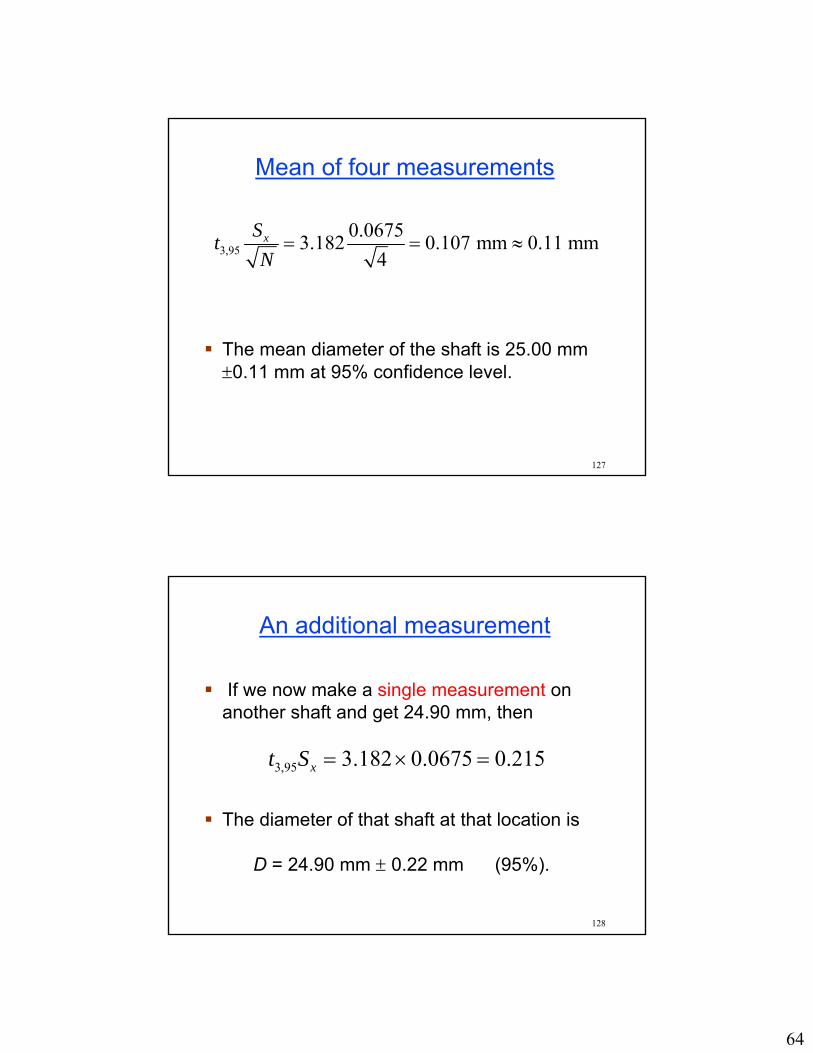
Mean of four measurements
The mean diameter of the shaft is 25.00 mm ±0.11 mm at 95% confidence level.
3,950.06753.182 0.107 mm 0.11 mm
4xStN
= = ≈
128
An additional measurement
If we now make a single measurement on another shaft and get 24.90 mm, then
The diameter of that shaft at that location is
D = 24.90 mm ± 0.22 mm (95%).
3,95 3.182 0.0675 0.215xt S = × =
65
129
Pooled StatisticsThis section just states that if you perform M separate identical
experiments, each consisting of N samples, you will get the same statistics as if you had a single experiment with M x Nmeasurements (seems pretty obvious ?)
130
Pooled Statistics
66
131
Chi-Squared Distribution (ki-squared)
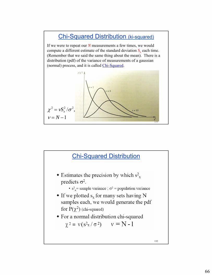
If we were to repeat our N measurements a few times, we would compute a different estimate of the standard deviation Sx each time. (Remember that we said the same thing about the mean). There is a distribution (pdf) of the variance of measurements of a gaussian(normal) process, and it is called Chi-Squared.
χ 2 = νSx2 /σ 2,
ν = N −1
132
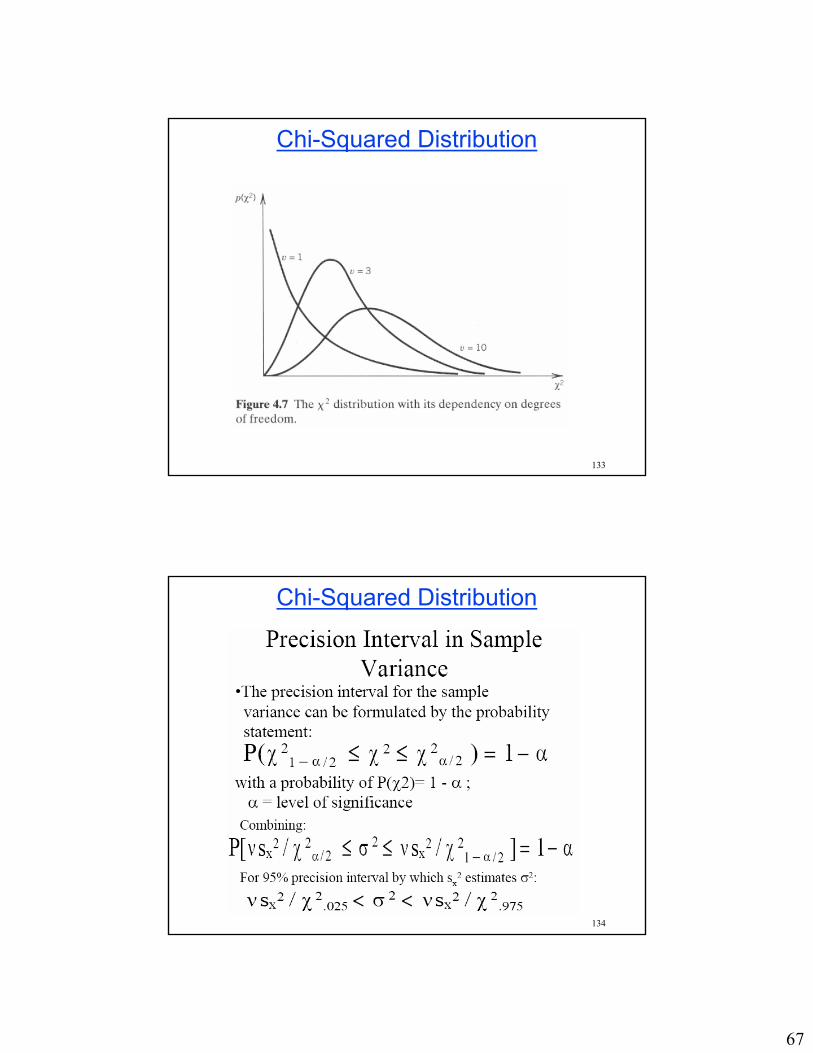
Chi-Squared Distribution
67
133
Chi-Squared Distribution
134
Chi-Squared Distribution

68
135
Chi-Squared Distribution
136
Chi-Squared Distribution
69
137
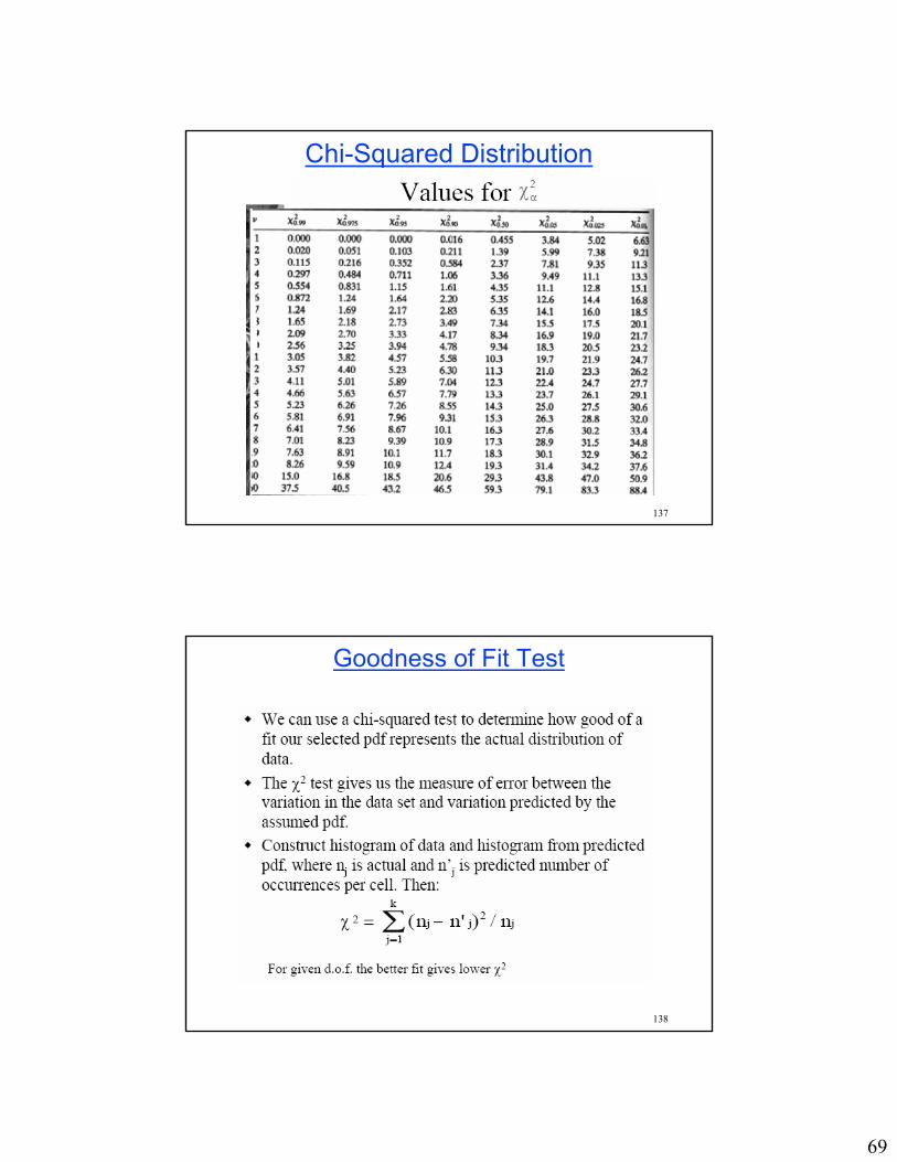
Chi-Squared Distribution
138
Goodness of Fit Test
N=64K = 7
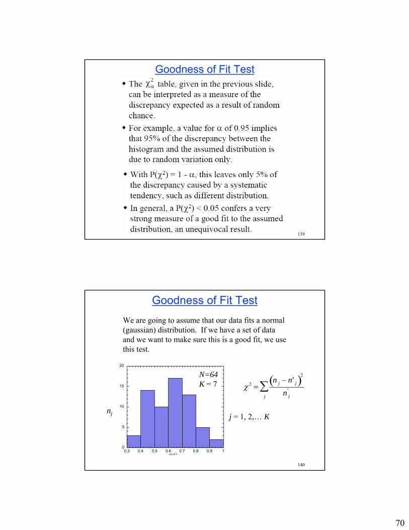
70
139
Goodness of Fit Test
140
Goodness of Fit TestWe are going to assume that our data fits a normal (gaussian) distribution. If we have a set of data and we want to make sure this is a good fit, we use this test.
0
5
10
15
20
0.3 0.4 0.5 0.6 0.7 0.8 0.9 1
Thermo II 2002
Cou
nt
out of 1
N=64K = 7
nj j = 1, 2,… K
χ 2 =n j − n' j( )2
n j'
j∑
71
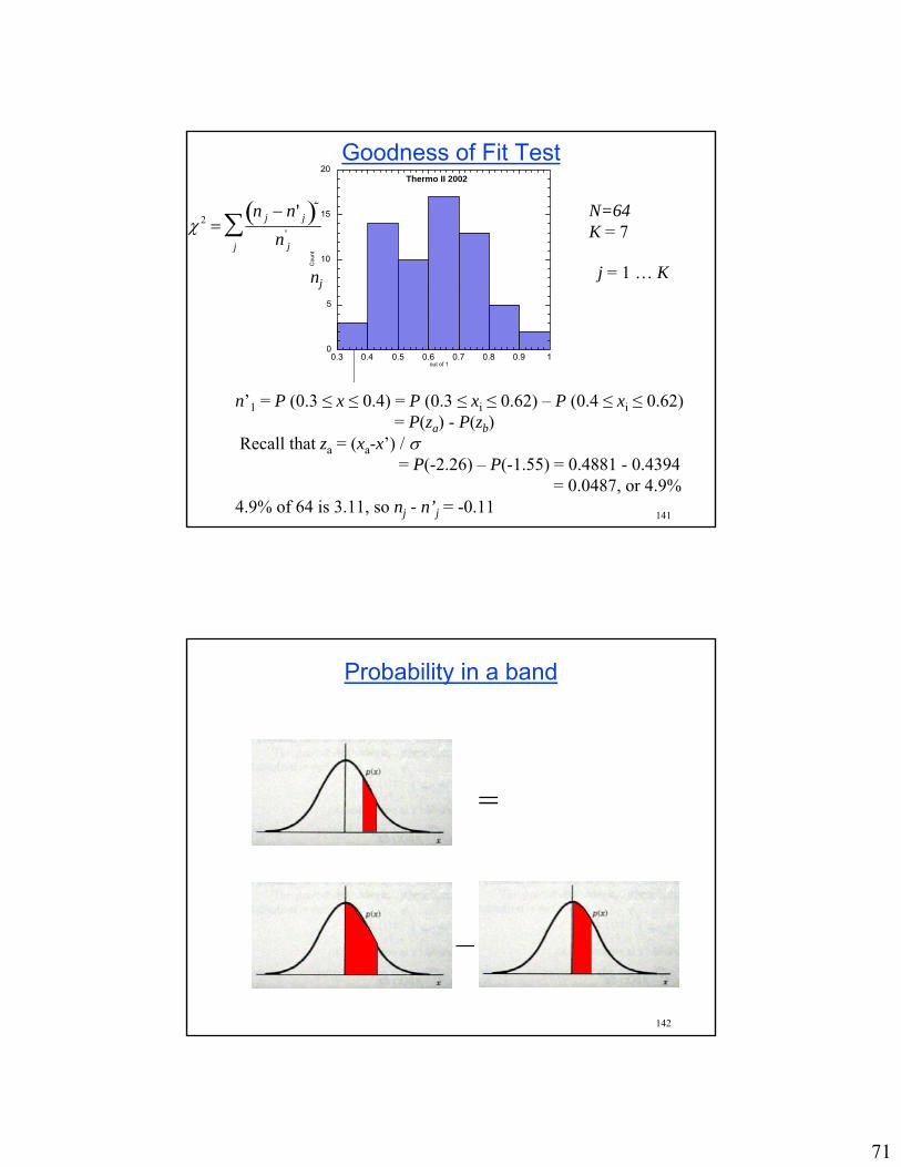
141
N=64K = 7
njj = 1 … K
x = 0.6196Sx = 0.14136
n’1 = P (0.3 ≤ x ≤ 0.4) = P (0.3 ≤ xi ≤ 0.62) – P (0.4 ≤ xi ≤ 0.62)= P(za) - P(zb)
Recall that za = (xa-x’) / σ= P(-2.26) – P(-1.55) = 0.4881 - 0.4394
= 0.0487, or 4.9%4.9% of 64 is 3.11, so nj - n’j = -0.11
χ 2 =n j − n' j( )2
n j'
j∑
Goodness of Fit Test
0
5
10
15
20
0.3 0.4 0.5 0.6 0.7 0.8 0.9 1
Thermo II 2002
Cou
nt
out of 1
142
Probability in a band
=
–
72
143
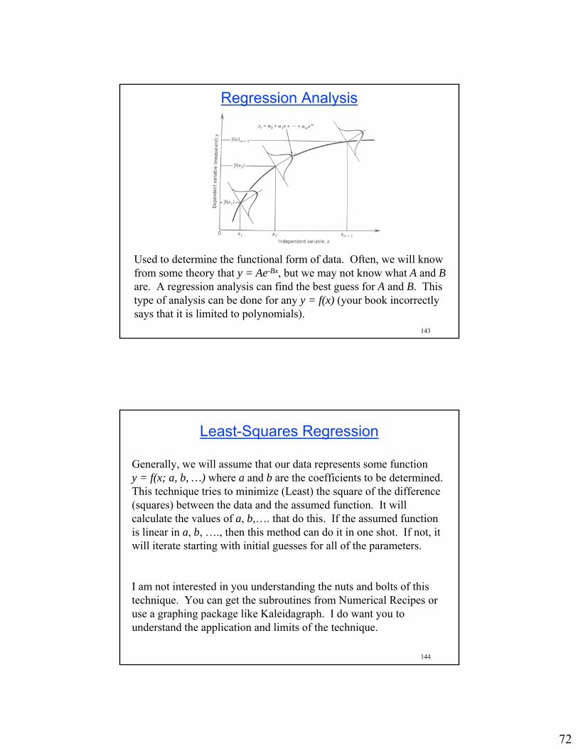
Regression Analysis
Used to determine the functional form of data. Often, we will know from some theory that y = Ae-Bx, but we may not know what A and Bare. A regression analysis can find the best guess for A and B. This type of analysis can be done for any y = f(x) (your book incorrectly says that it is limited to polynomials).
144
Least-Squares Regression
Generally, we will assume that our data represents some functiony = f(x; a, b, …) where a and b are the coefficients to be determined. This technique tries to minimize (Least) the square of the difference (squares) between the data and the assumed function. It will calculate the values of a, b,…. that do this. If the assumed function is linear in a, b, …., then this method can do it in one shot. If not, it will iterate starting with initial guesses for all of the parameters.
I am not interested in you understanding the nuts and bolts of this technique. You can get the subroutines from Numerical Recipes or use a graphing package like Kaleidagraph. I do want you to understand the application and limits of the technique.

73
145
Curve Fitting Examples
146
Number of Measurements Required
Again, the books discussion on this topic is confusing since it uses a t-estimator. There is nothing wrong with this approach, but it isperhaps easier to understand using infinite statistics. Say we have a measurement of some random data, and we want to know its mean with an error smaller than 5%. If we have some estimate of its standard deviation, then we know that
The above statement says that we want to be less than 5% of
Sx =Sx
N 1 / 2
Sx x 0.05 = Sx / x = Sx
x N 1 / 2
N =Sx
0.05 x ⎛ ⎝ ⎜
⎞ ⎠ ⎟
2
74
147
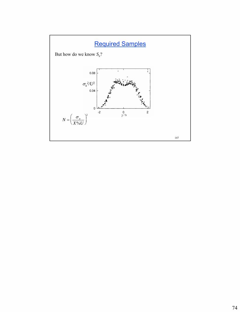
Required SamplesBut how do we know Sx?
σu2/U2
N =σ u
X%U⎛ ⎝ ⎜
⎞ ⎠ ⎟
2


![TIMOTHY BESLEY AND ANNE CASE - Princeton Universityaccase/downloads/Does...and voters. Besley and Case [1995] have extended the basic model to permit yardstick competition in tax setting](https://img.pdfslide.us/doc/110x75/60b2a94964ffb86809729732/timothy-besley-and-anne-case-princeton-university-accasedownloadsdoes-and.jpg)