Bergals School of Economics Fall 1997/8Tel Aviv University

Second degree price discrimination

Yossi Spiegel

1. Introduction

Second degree price discrimination refers to cases where a firm does not have precise information

about the preferences of individual customers but it can use non-linear tariffs in order to extract

the relevant information from its customers. At the optimum, the firm typically offers a menu

of offers and buyers self-select from this menu. Second degree price discrimination is

undoubtedly much more complex to analyze than first degree or third degree price discrimination.

This is because the combination of non linear tariffs and asymmetric information about buyers

requires certain techniques to solve the firm’s problem. These techniques were not available until

the early 70’s. The major breakthrough was by Mirrlees in his 1971 paper about non linear

taxation under asymmetric information. In 1996 Mirrlees got the Nobel prize for this

contribution. The methodology that Mirrlees developed is the basis for the analysis of second

degree price discrimination. Since this methodology is so widely used we shall study it in detail.

2. The model

A monopoly sells a single product to a continuum of buyers. Buyers differ from one another

with respect to their utilities: the utility of a representative buyer if he buys is given by

where p is the price andθ is the buyer’s type. If a buyer does not buy his utility is 0. As for

(1)

q, we can give this parameter at least two interpretations. First we can think of q as a quantity

(i.e., the number of units the buyer buys). In that case, p is the price of a bundle that contains

q units and V(q,θ) is the gross consumer surplus (i.e., the area under the inverse demand

function). This interpretation corresponds to Maskin and Riley’s (1984) paper. Second we can

think of q as a measure of the quality of the product. Under this interpretation, each buyer is

2

interested in buying only one unit, p is the price of that unit, and V(q,θ) is the direct utility from

consumption, ignoring the loss of income due to the payment to the monopoly. The

interpretation of q as quality corresponds to Mussa and Rosen’s (1978) paper. As usual, we will

assume that Vq > 0 > Vqq so the direct utility from consumption increases with q (the number of

units the buyer buys or the quality of the good he buys) at a decreasing rate. Since Vq is the

marginal willingness to pay, then if we interpret q is quantity then Vq is simply the inverse

demand function so the assumptions that Vq > 0 > Vqq amount to assuming that the inverse

demand function is positive and decreasing.1 Similarly, if we interpret q is quality, the

assumption that Vq > 0 > Vqq implies that the inverse demand function for quality is positive and

decreasing.

The variableθ (the buyer’s type) is distributed on the interval [θ0, θ1] according to a

distribution function f(θ) and a cumulative distribution function F(θ). Assume that Vθ > 0 and

Vqθ > 0 so higher types have higher utility levels and higher marginal utilities.2 Since Vq can

be thought of as the inverse demand function, the assumption that Vqθ > 0 means that higher

types have higher demand functions. This assumption is important because it guarantees that the

inverse demand functions for two different types never cross one another. In addition we will

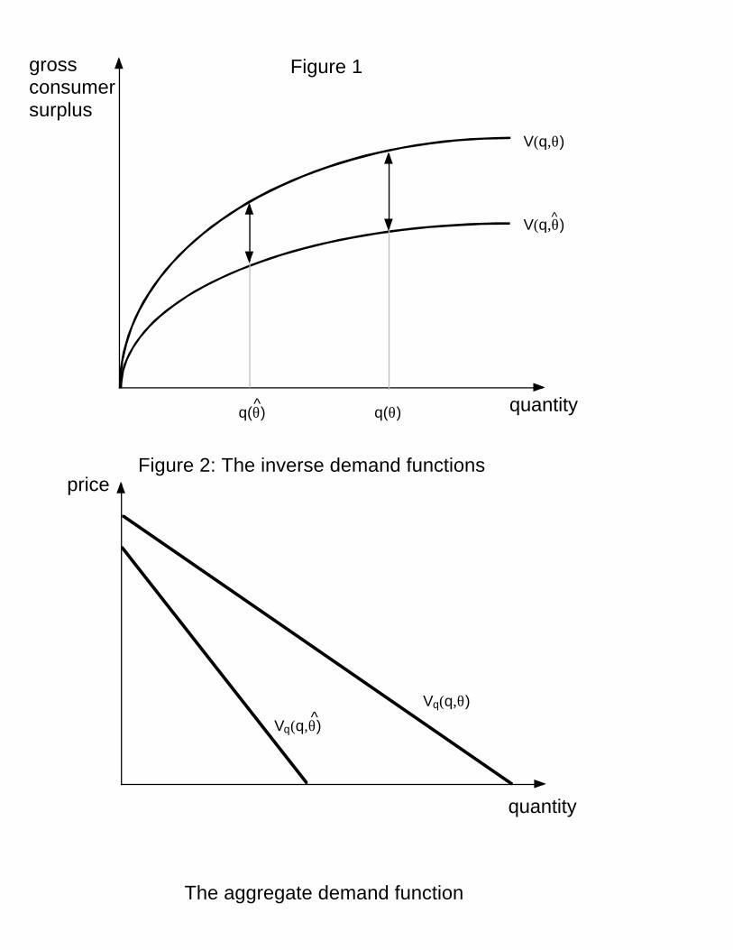
assume that Vqqθ ≤ 0. Keeping in mind the interpretation of Vq as the inverse demand function,

the assumption that Vqqθ ≤ 0 means that the slope of the inverse demand functions is steeper for

lower types. This situation is shown in Figure 2.

The firm has a the same cost for serving each buyer (so there is no interaction between

different buyers through the monopoly’s cost like in the case of third degree price

discrimination). The cost of serving a buyer depends on q and it is given by c(q), where c’ >

0, c" ≥ 0. Hence, if we adopt the interpretation of q as quality, this assumption means that it is

1 Note that given a uniform price, a buyer’s utility is given by V(q,θ)-pq. The quantity thatthe buyer would like to buy at that price is given implicitly by Vq(q,θ) = p. The equation canbe also interpreted as describing the highest price that the buyer will agree to pay when healready buys q units. This is by definition the inverse demand function of the buyer.

2 If the utility of the buyer when he does not buy is not 0 as I have assumed above (i.e.,V(0,θ) ≠ 0), then the assumption that Vθ > 0 should be replaced with the assumption thatd/dθ(V(q,θ)-V(0,θ)) = Vθ(q,θ)-Vθ(0,θ) > 0 for all q > 0.

price

gross consumer surplus

quantity

quantity

Figure 2: The inverse demand functions

V(q,θ)

The aggregate demand function

V(q,θ)^

Figure 1

q(θ)q(θ)^

Vq(q,θ)

Vq(q,θ)̂

3

more costly to produce higher quality products and the marginal cost increases at an increasing

rate. When we’ll treat q as quantity in a bundle, it will be more natural to assume that c" = 0.

(It is hard to believe that a 2 liter bottle costs to produce more than twice than a one liter bottle -

in fact quite the opposite might be true. But to keep up with the assumption that c"≥ 0 which

is natural in the case of quality, let’s assume that when q is quantity, c" = 0.)

3. The full information benchmark

When the monopoly knows the buyers’ type, we are in a situation of first degree price

discrimination. The monopoly’s problem then is as follows:

That is the monopoly maximizes profits subject to the constraint that the buyer will buy. Clearly

(2)

at the optimum it must be the case that the constraint holds with equality otherwise the monopoly

can raise p and make more money. Substituting from the constraint into the objective function

and maximizing with respect to q, the optimal q is given implicitly by the following first-order

condition:

Let q*(θ) be the solution to this equation. The optimal price is then given by p*(θ) = V(q*(θ),θ).

(3)

Equation (3) shows that at the optimum the monopoly equates the marginal benefit of the

consumer from q with the marginal cost of q. The choice of q is socially optimal because the

monopoly captures the entire social surplus by making sure that at the optimum the buyer makes

zero utility and is just indifferent between buying and not buying.

4. Asymmetric information

Now suppose that the buyer’s type is private information (i.e., only the buyer knows his ownθ).

The monopoly only knows the distribution of types but cannot tell the type of an individual

4

buyer. In order to find out the prices and quantities/qualities that the monopoly will offer we will

model the situation as a Bayesian game. In this game, the monopoly chooses a menu of price

and quantity/quality pairs, and each buyer selects at most one pair from the menu. If a buyer

does not select any pair from the menu, he does not buy anything and does not pay anything.

But if he selects the pair (p, q), then he pays the monopoly p and gets in return a quantity/quality

q. Since the monopoly can put himself in the buyers shoes, he anticipates their selections for

every menu he offers them. Therefore, we can characterize the optimal menu offered by the

monopoly by using the revelation approach which is the standard way to solve these kind of

problems. According to this approach, instead of offering the buyers a menu with pairs of p and

q, the monopoly can ask each buyer for his type and select for the buyer the pair that the buyer

whose type coincides with the report would have selected in the original game. To illustrate,

suppose that in the original game, a buyer whose type isθ’ chose the pair (p’, q’). Now in the

revelation game, if a buyer will report that his type isθ’ the monopoly will select for him the

pair (p’, q’). Of course if some type, sayθ", chose not to select anything from the original

menu, the monopoly will select nothing for buyers who will report that their type isθ".

In short, the monopoly will design a menu of price and quantity/quality pairs, (p(θ), q(θ)),

such that each pair will be geared towards one type of a buyer. Then each buyer will report his

type to the monopoly, and the monopoly will then charge him the price and will give him the

quantity/quality that was designed that reported type. The monopoly’s strategy along with the

buyer’s report are referred to as a mechanism and will be denoted by M = {p(θ), q(θ), θ ∈ [θ0,

θ1]}.

In order to find the optimal mechanism from the monopoly’s point of view, we can

invoke the revelation principle. This principle says that we can restrict attention to mechanisms

in which the buyers report their types truthfully.3 Such mechanisms are calledIncentive

3 This of course does not mean that the buyers will always report their types truthfully. Itonly means that at the optimum there is no loss of generality in looking at mechanisms in whichthey do report their types truthfully. The reason for this is straightforward: suppose that we hada mechanism in which the monopoly offers buyers a menu that contains pairs of p and q andeach buyer selects one pair from this menu. Suppose that among all possible such mechanism(all the possible menus of pairs of p and q) there is one that is best for the monopoly andsuppose moreover that in this optimal mechanism, the buyer whose type isθ’ selects the pair (p’,

5

Compatible (IC) and they satisfy the following set of (IC) constraints:

The IC constraints state the each buyer is better-off reporting his type truthfully than pretending

(4)

to be some other type. Or using an alternative interpretation, each type prefers to pick the pair

that geared towards him than picking any other pair. Since buyers can always get a zero level

of utility it must be the case that

These type of constraints are calledIndividual Rationality (IR) or Voluntary Participation

(5)

(VP) constraints. A mechanism is said to befeasible is it satisfies the IC and IR constraints.

4.1 The monopoly’s problem

Given an incentive compatible mechanism M = {p(θ), q(θ), θ ∈ [θ0, θ1]}, the monopoly’s

problem is to solve the following problem:

q’). Since the monopoly can always puts himself in the buyers’ shoes, he realizes that this iswhat the buyer will do, so he can design an equivalent revelation mechanism. In this mechanism,each buyer announces his type to the monopoly and the monopoly in turn selects for the buyera pair of p and q from the menu, based on the buyers report. The monopoly can always designthis revelation mechanism in such a way that once a buyer announces that his type isθ’ he getsthe pair (p’, q’). That is, the monopoly designs the new mechanism such that p(θ’) = p’ andq(θ’) = q’. Since typeθ’ selects the pair (p’, q’) in the original game he will have an incentiveto report his true type in the revelation mechanism in order to receive again the pair (p’ q’)which is the most preferred pair from his point of view. Hence, the monopoly can design therevelation mechanism in a way that leads to exactly the same outcome as in the originalmechanism. Since the original mechanism was the best from the monopoly’s point of view, sowill be the new mechanism. Note that in the new mechanism, each buyer reports his typetruthfully, since otherwise he gets a pair that is not optimal from his point of view.

6

In general the problem is very messy. Hence we shall now simplify it in order to characterize

(6)

the optimal menu that the monopoly will offer. We will do so by simplifying the IC and IR

constraints in a series of claims. This will enable us in the end to solve a much simpler problem.

This approach follows the methodology developed by Baron and Myerson’s (1982) classic paper

on optimal regulation under asymmetric information (see also Baron 1989).

4.2 Simplifying the constraints

Claim 1: IC implies that U(θ) is monotonically increasing, so U(θ0) ≥ 0 is sufficient to ensure

that all the IR constraint are satisfied.

Proof of Claim 1: Using IC and recalling that Vθ > 0, it follows that for allθ > θ0:

Hence if IR holds for typeθ0, it surely holds for all types greater thanθ0.

(7)

Remark: Claim 1 implies that we can replace all IR constraints with the single constraint U(θ0)

≥ 0. Moreover, we can already tell that at the optimum it must be the case that U(θ)0 = 0,

otherwise the monopoly can raise p(θ0) further.

Claim 2: Incentive compatibility implies

where U(θ0) is the utility of the lowest type of the buyer.

(8)

7

Remark: The first term on the right side of equation (8) is referred to in the literature as the

"information rent" of the typeθ buyer because we know that under full information each buyer

gets a zero utility. Thus the buyers can have a positive surplus only because the monopoly needs

to "bribe" them in order to induce them to reveal their private information regarding their types.

Proof of Claim 2: Suppose that typeθ̂ reports truthfully. Then, his utility is

Using this expression, the IC constraint for typeθ can be written as

(9)

Similarly, the IC constraint of typeθ̂ can be written as

(10)

Combining the inequalities (10) and (11) we get

(11)

Assuming without a loss of generality thatθ > θ̂, dividing the inequalities byθ-θ̂ and taking the

(12)

limit as θ-θ̂ goes to zero yields

almost everywhere. Since by assumption, Vθ > 0, equation (13) shows that, as we found in

(13)

Claim 1, higher types indeed get a higher level of utility at the optimum. Thus, we can integrate

(13) from θ0 to θ to obtain equation (8).

Remark: If we assume that p(θ) and q(θ) are differentiable, we can derive equation (13) more

easily from the IC constraints. To see how, note that incentive compatibility means that

8

That is, the best thing that a buyer can do is to report his type truthfully. Therefore it must be

(14)

the case that

Differentiating U(θ) with respect toθ and using this equation, yields equation (13). The proof

(15)

of the claim is more general however because it does not rely on the assumption that q(θ) and

p(θ) are differentiable. Indeed one of the purposes of the proof is to establish that U(θ) is

differentiable almost everywhere.

Claim 3: IC implies that

where U(θ0) = 0 is the utility of the lowest type.

(16)

Proof of Claim 3: Equation (16) can be derived from equations (1) and (13). Now let’s verify

that p(θ) indeed induces truthful revelation. To this end, suppose that a buyer whose true type

is θ reports that his type isθ̂ and buys according to the pair (p(θ̂), q(θ̂)). The buyer’s utility then

is given by

The optimal report for the buyer is given by the following first-order condition:

(17)

9

This equation implies that at a local optimum,θ̂ = θ, so the buyer will indeed have an incentive

(18)

to report his type truthfully at least locally. Truthful revelation is optimal at this point only

locally because we did not show up to now thatθ̂ = θ is a global optimum (indeed we are yet

to show that the second order condition is satisfied).

Claim 4: A monotonically increasing q(θ) is a necessary and sufficient condition for truthful

revelation to be globally optimal.

Remark: Claim 4 establishes that any mechanism such that the q(θ) is monotonically increasing

in θ is incentive compatible. This claim simplifies the monopoly’s problem immensely since it

will allow us to replace the IC constraints with the constraint that q(θ) must be an increasing

function (in fact we will not even do that: we will simply solve an unconstrained maximization

problem and then verify that the optimal q(θ) is monotonically increasing inθ). It implies that

higher types buy bigger bundles or if q represents quality, they buy better products. Of course,

it can’t be that higher types get higher q and pay lower prices as this would give lower types an

incentive to mimic them, thus violating IC. This can be verified by differentiating p(θ) with

respect toθ:

which is positive when q’(θ) > 0.

(19)

Proof of Claim 4: First we will show that a necessary condition for global incentive

compatibility is that q(θ) is a monotonically increasing function. From (12) we know that for

all θ̂, θ ∈ [θ0, θ1], the following inequality must hold if the mechanism is incentive compatible:

Now assume without a loss of generality thatθ > θ̂. Because Vθ > 0, both sides of the inequality

(20)

10

are positive. Moreover because Vqθ > 0, the left side can exceed the right side only if q(θ) >

q(θ̂). Hence, we showed that global incentive compatibility is satisfied only if q(θ) is a

monotonically increasing function.

Next we will show that the necessary condition is also sufficient. In other words, we need

to show that if q(θ) is a monotonically increasing function then the IC constraints given by (4)

hold. To this end, assuming again (without a loss of generality) thatθ > θ̂, and subtracting

equation (17) from (8) yields,

Since Vqθ > 0 it is clear that q(θ) > q(θ̂) ensures that U(θ) - U(θ̂ θ) > 0 so themonotonicity of

(21)

q(θ) is also a sufficient condition for global incentive compatibility.

The first part of Claim 4 is demonstrated in Figure 1. The two sides of inequality (20)

describe the vertical distance between the gross consumer surpluses of two buyers and are

represented by the two arrows. Given thatθ > θ̂, we know that from the assumption that Vθ >

0, that the gross consumer surplus of theθ type buyer lies above the gross consumer surplus of

the θ̂ type buyer. Moreover, from the assumption that Vqθ > 0, we also know that the vertical

distance between the two curves must increase as we move to the right since V(.,θ) is steeper

than V(.,θ̂). Consequently, inequality (20) can hold only if q(θ) > q(θ̂). Graphically, the

properties of the gross consumer surplus imply that the left arrow in Figure 1 is shorter than the

right arrow so it must be that q(θ) > q(θ̂).

4.3 Rewriting the monopoly’s maximization problem

Having simplified the set of constraints, we are now in a position to rewrite the monopoly’s

problem. Since U(θ0) = 0 is sufficient to ensure that all IR constraints hold and since requiring

that q(θ) is a monotonically increasing function is necessary and sufficient for global incentive

11

compatibility, the monopoly’s problem can be rewritten as follows:

Substituting from equation (16) for p(θ) into the objective function and imposing the constraint

(22)

that U(θ0) = 0, the monopoly’s problem becomes:

We therefore turned the problem into a problem of finding an optimal function, q(θ), subject to

(23)

a monotonicity constraint. The common "trick" now (due to Mirrlees, 1971) is to ignore the

constraint, solve the problem and verify later that the solution satisfies the constraint. But before

we solve the problem we can simplify it a bit further. To this end note that after integration by

parts, the expression

becomes

(24)

12

Substituting this expression in (23), the monopoly’s problem becomes:

(25)

where

(26)

(27)

4.4 The optimal menu

Let q*(θ) be the solution to the monopoly’s maximization problem written in (26). We can solve

for q*(θ) by maximizing the integral in (26) pointwise. That is, for everyθ, q*(θ) is the value

of q that maximizes the expression I(q(θ),θ). Since we repeat this procedure for every value of

θ we obtain the optimal q as a function ofθ. Pointwise maximization is possible since there is

no "interaction" between the optimal choices for different types in the sense that the integrand

in (26) involve terms that depend only on one value ofθ. The first order condition for an

interior solution for q*(θ) is

where H(θ) ≡ (1-F(θ))/f(θ) is the inverse of the "hazard rate" of the distribution ofθ. The left

(28)

side of the equation is simply the marginal willingness of the buyer to pay for an extra unit of

13

q (or the inverse demand function of the buyer). The first expression is the marginal cost of an

extra unit of q. These two expression are exactly the same as in the full information case. The

difference between the current case and the full information case is that we now have an

additional term on the right side of the equation which represents an additional cost from the

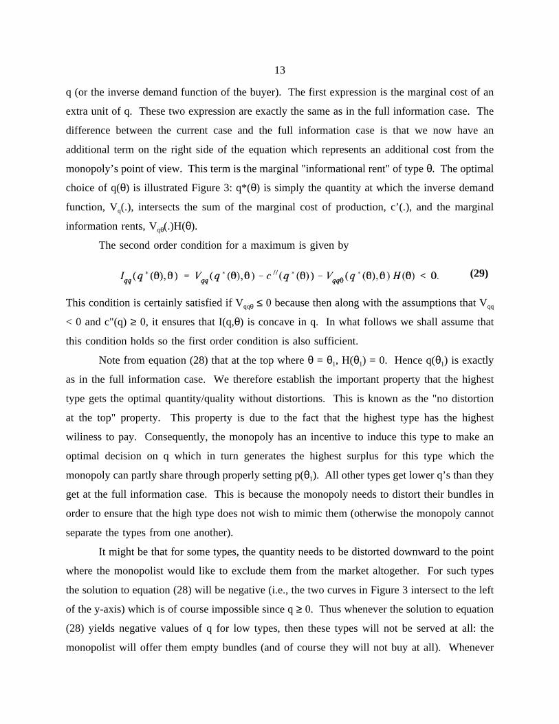
monopoly’s point of view. This term is the marginal "informational rent" of typeθ. The optimal

choice of q(θ) is illustrated Figure 3: q*(θ) is simply the quantity at which the inverse demand

function, Vq(.), intersects the sum of the marginal cost of production, c’(.), and the marginal

information rents, Vqθ(.)H(θ).

The second order condition for a maximum is given by

This condition is certainly satisfied if Vqqθ ≤ 0 because then along with the assumptions that Vqq

(29)

< 0 and c"(q)≥ 0, it ensures that I(q,θ) is concave in q. In what follows we shall assume that

this condition holds so the first order condition is also sufficient.

Note from equation (28) that at the top whereθ = θ1, H(θ1) = 0. Hence q(θ1) is exactly

as in the full information case. We therefore establish the important property that the highest

type gets the optimal quantity/quality without distortions. This is known as the "no distortion

at the top" property. This property is due to the fact that the highest type has the highest

wiliness to pay. Consequently, the monopoly has an incentive to induce this type to make an

optimal decision on q which in turn generates the highest surplus for this type which the

monopoly can partly share through properly setting p(θ1). All other types get lower q’s than they

get at the full information case. This is because the monopoly needs to distort their bundles in

order to ensure that the high type does not wish to mimic them (otherwise the monopoly cannot

separate the types from one another).

It might be that for some types, the quantity needs to be distorted downward to the point

where the monopolist would like to exclude them from the market altogether. For such types

the solution to equation (28) will be negative (i.e., the two curves in Figure 3 intersect to the left

of the y-axis) which is of course impossible since q≥ 0. Thus whenever the solution to equation

(28) yields negative values of q for low types, then these types will not be served at all: the

monopolist will offer them empty bundles (and of course they will not buy at all). Whenever

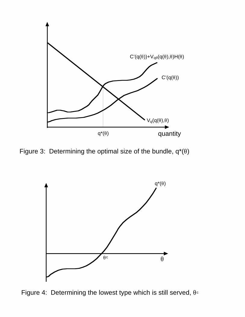
Figure 3: Determining the optimal size of the bundle, q*(θ)

quantity

C’(q(θ))+Vqθ(q(θ),θ)H(θ)

q*(θ)

Vq(q(θ),θ)

C’(q(θ))

θc θ

q*(θ)

Figure 4: Determining the lowest type which is still served, θc

14

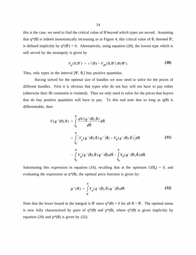
this is the case, we need to find the critical value ofθ beyond which types are served. Assuming

that q*(θ) is indeed monotonically increasing as in Figure 4, this critical value ofθ, denotedθc,

is defined implicitly by q*(θc) = 0. Alternatively, using equation (28), the lowest type which is

still served by the monopoly is given by

Thus, only types in the interval [θc, θ1] buy positive quantities.

(30)

Having solved for the optimal size of bundles we now need to solve for the prices of

different bundles. First it is obvious that types who do not buy will not have to pay either

(otherwise their IR constraint is violated). Thus we only need to solve for the prices that buyers

that do buy positive quantities will have to pay. To this end note that so long as q(θ) is

differentiable, then

Substituting this expression in equation (16), recalling that at the optimum U(θ0) = 0, and

(31)

evaluating the expression at q*(θ), the optimal price function is given by:

Note that the lower bound in the integral isθc since q*(θ) = 0 for all θ < θc. The optimal menu

(32)

is now fully characterized by pairs of q*(θ) and p*(θ), where q*(θ) is given implicitly by

equation (28) and p*(θ) is given by (32).

15

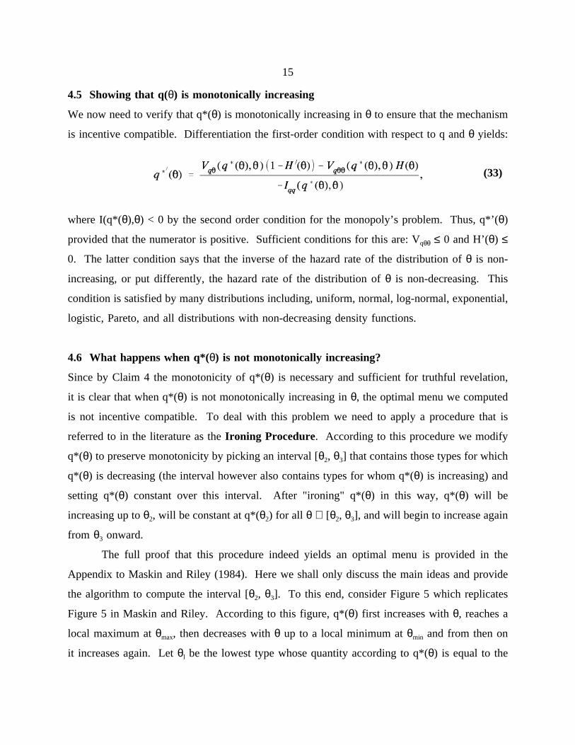
4.5 Showing that q(θ) is monotonically increasing

We now need to verify that q*(θ) is monotonically increasing inθ to ensure that the mechanism

is incentive compatible. Differentiation the first-order condition with respect to q andθ yields:

where I(q*(θ),θ) < 0 by the second order condition for the monopoly’s problem. Thus, q*’(θ)

(33)

provided that the numerator is positive. Sufficient conditions for this are: Vqθθ ≤ 0 and H’(θ) ≤

0. The latter condition says that the inverse of the hazard rate of the distribution ofθ is non-

increasing, or put differently, the hazard rate of the distribution ofθ is non-decreasing. This

condition is satisfied by many distributions including, uniform, normal, log-normal, exponential,

logistic, Pareto, and all distributions with non-decreasing density functions.

4.6 What happens when q*(θ) is not monotonically increasing?

Since by Claim 4 the monotonicity of q*(θ) is necessary and sufficient for truthful revelation,

it is clear that when q*(θ) is not monotonically increasing inθ, the optimal menu we computed

is not incentive compatible. To deal with this problem we need to apply a procedure that is

referred to in the literature as theIroning Procedure. According to this procedure we modify

q*(θ) to preserve monotonicity by picking an interval [θ2, θ3] that contains those types for which

q*(θ) is decreasing (the interval however also contains types for whom q*(θ) is increasing) and

setting q*(θ) constant over this interval. After "ironing" q*(θ) in this way, q*(θ) will be

increasing up toθ2, will be constant at q*(θ2) for all θ ∈ [θ2, θ3], and will begin to increase again

from θ3 onward.

The full proof that this procedure indeed yields an optimal menu is provided in the

Appendix to Maskin and Riley (1984). Here we shall only discuss the main ideas and provide

the algorithm to compute the interval [θ2, θ3]. To this end, consider Figure 5 which replicates

Figure 5 in Maskin and Riley. According to this figure, q*(θ) first increases withθ, reaches a

local maximum atθmax, then decreases withθ up to a local minimum atθmin and from then on

it increases again. Letθl be the lowest type whose quantity according to q*(θ) is equal to the

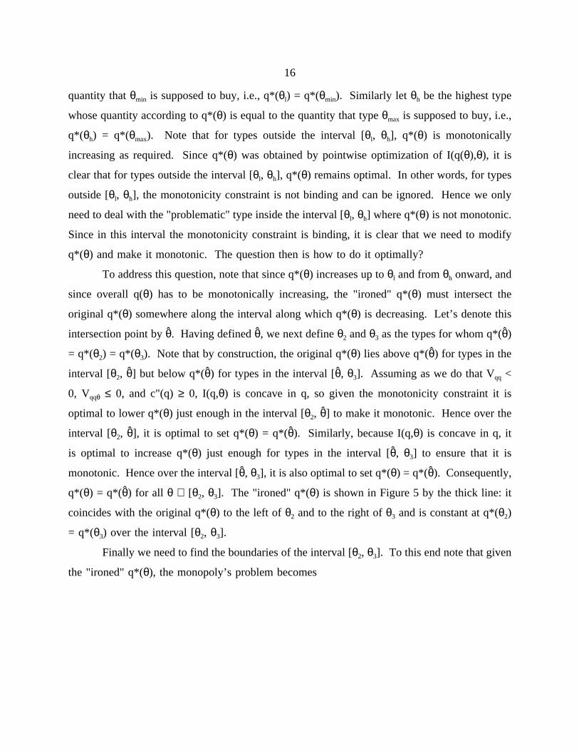
16

quantity thatθmin is supposed to buy, i.e., q*(θl) = q*(θmin). Similarly let θh be the highest type

whose quantity according to q*(θ) is equal to the quantity that typeθmax is supposed to buy, i.e.,

q*(θh) = q*(θmax). Note that for types outside the interval [θl, θh], q*(θ) is monotonically

increasing as required. Since q*(θ) was obtained by pointwise optimization of I(q(θ),θ), it is

clear that for types outside the interval [θl, θh], q*(θ) remains optimal. In other words, for types

outside [θl, θh], the monotonicity constraint is not binding and can be ignored. Hence we only

need to deal with the "problematic" type inside the interval [θl, θh] where q*(θ) is not monotonic.

Since in this interval the monotonicity constraint is binding, it is clear that we need to modify

q*(θ) and make it monotonic. The question then is how to do it optimally?

To address this question, note that since q*(θ) increases up toθl and fromθh onward, and

since overall q(θ) has to be monotonically increasing, the "ironed" q*(θ) must intersect the

original q*(θ) somewhere along the interval along which q*(θ) is decreasing. Let’s denote this

intersection point byθ̂. Having definedθ̂, we next defineθ2 andθ3 as the types for whom q*(θ̂)

= q*(θ2) = q*(θ3). Note that by construction, the original q*(θ) lies above q*(θ̂) for types in the

interval [θ2, θ̂] but below q*(θ̂) for types in the interval [θ̂, θ3]. Assuming as we do that Vqq <

0, Vqqθ ≤ 0, and c"(q)≥ 0, I(q,θ) is concave in q, so given the monotonicity constraint it is

optimal to lower q*(θ) just enough in the interval [θ2, θ̂] to make it monotonic. Hence over the

interval [θ2, θ̂], it is optimal to set q*(θ) = q*(θ̂). Similarly, because I(q,θ) is concave in q, it

is optimal to increase q*(θ) just enough for types in the interval [θ̂, θ3] to ensure that it is

monotonic. Hence over the interval [θ̂, θ3], it is also optimal to set q*(θ) = q*(θ̂). Consequently,

q*(θ) = q*(θ̂) for all θ ∈ [θ2, θ3]. The "ironed" q*(θ) is shown in Figure 5 by the thick line: it

coincides with the original q*(θ) to the left ofθ2 and to the right ofθ3 and is constant at q*(θ2)

= q*(θ3) over the interval [θ2, θ3].

Finally we need to find the boundaries of the interval [θ2, θ3]. To this end note that given

the "ironed" q*(θ), the monopoly’s problem becomes

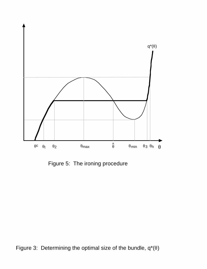
Figure 5: The ironing procedure

θ

q*(θ)

Figure 3: Determining the optimal size of the bundle, q*(θ)

θl θhθ2 θ3θ̂θc θmax θmin

17

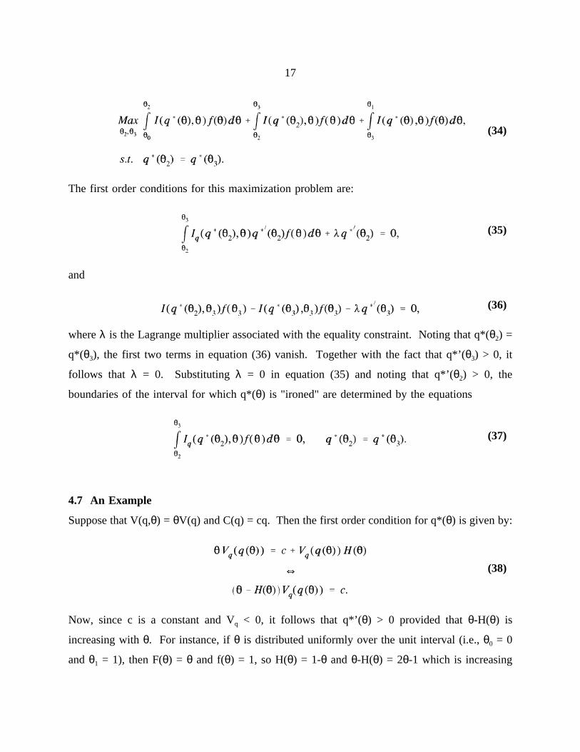
The first order conditions for this maximization problem are:

(34)

and

(35)

whereλ is the Lagrange multiplier associated with the equality constraint. Noting that q*(θ2) =

(36)

q*(θ3), the first two terms in equation (36) vanish. Together with the fact that q*’(θ3) > 0, it

follows that λ = 0. Substitutingλ = 0 in equation (35) and noting that q*’(θ2) > 0, the

boundaries of the interval for which q*(θ) is "ironed" are determined by the equations

(37)

4.7 An Example

Suppose that V(q,θ) = θV(q) and C(q) = cq. Then the first order condition for q*(θ) is given by:

Now, since c is a constant and Vq < 0, it follows that q*’(θ) > 0 provided thatθ-H(θ) is

(38)

increasing withθ. For instance, ifθ is distributed uniformly over the unit interval (i.e.,θ0 = 0

andθ1 = 1), then F(θ) = θ and f(θ) = 1, so H(θ) = 1-θ andθ-H(θ) = 2θ-1 which is increasing

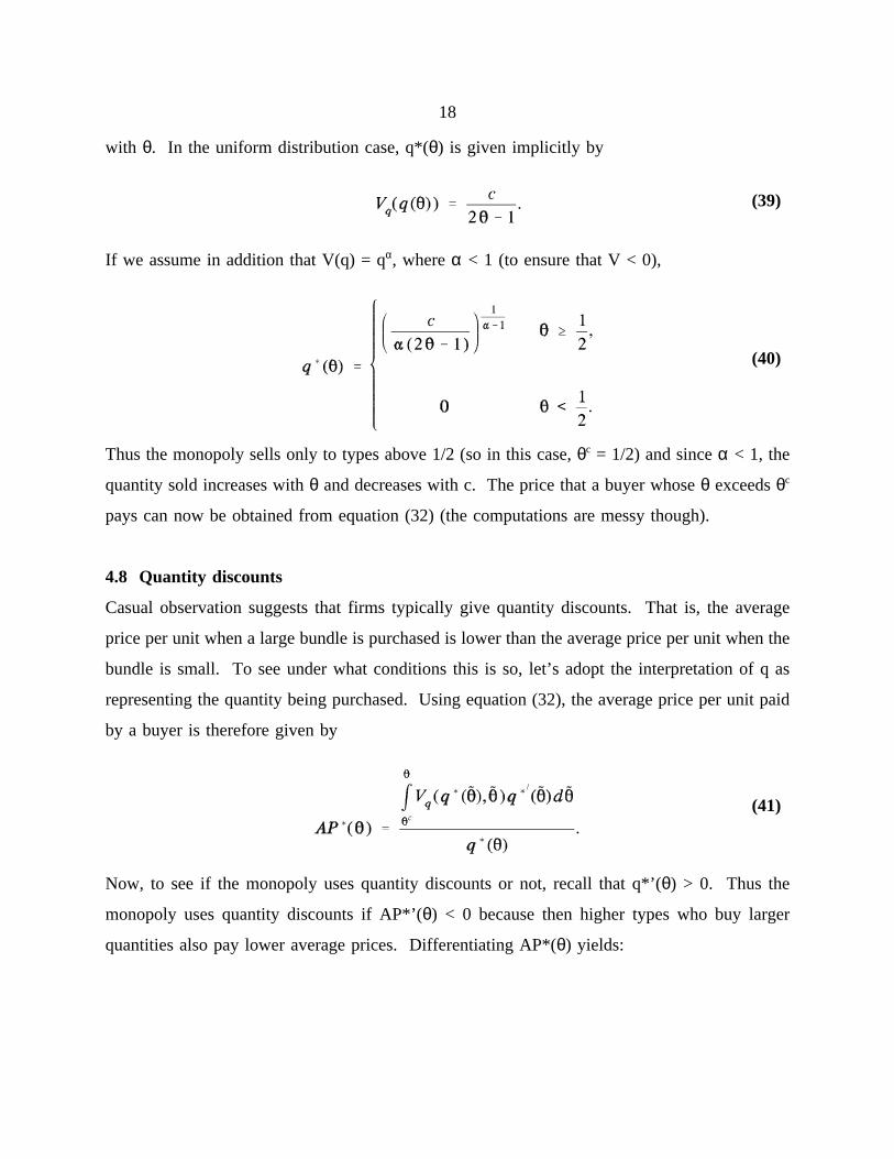
18

with θ. In the uniform distribution case, q*(θ) is given implicitly by

If we assume in addition that V(q) = qα, whereα < 1 (to ensure that V < 0),

(39)

Thus the monopoly sells only to types above 1/2 (so in this case,θc = 1/2) and sinceα < 1, the

(40)

quantity sold increases withθ and decreases with c. The price that a buyer whoseθ exceedsθc

pays can now be obtained from equation (32) (the computations are messy though).

4.8 Quantity discounts

Casual observation suggests that firms typically give quantity discounts. That is, the average

price per unit when a large bundle is purchased is lower than the average price per unit when the

bundle is small. To see under what conditions this is so, let’s adopt the interpretation of q as

representing the quantity being purchased. Using equation (32), the average price per unit paid

by a buyer is therefore given by

Now, to see if the monopoly uses quantity discounts or not, recall that q*’(θ) > 0. Thus the

(41)

monopoly uses quantity discounts if AP*’(θ) < 0 because then higher types who buy larger

quantities also pay lower average prices. Differentiating AP*(θ) yields:

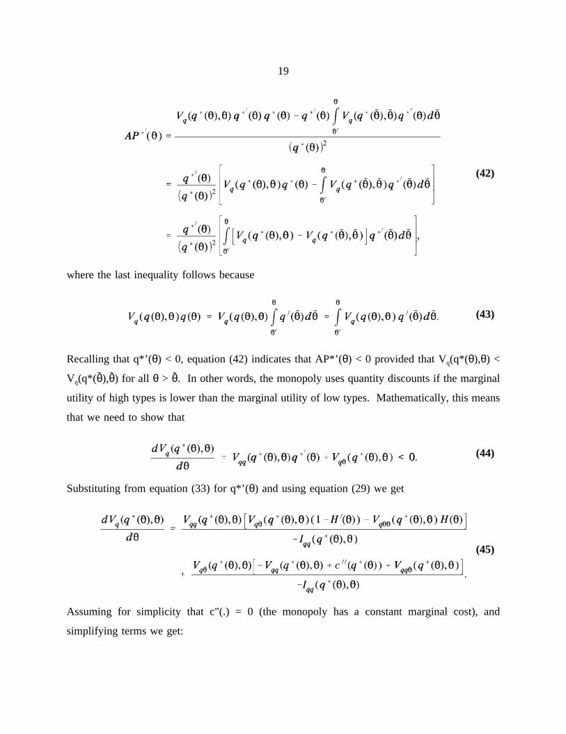
19

where the last inequality follows because

(42)

Recalling that q*’(θ) < 0, equation (42) indicates that AP*’(θ) < 0 provided that Vq(q*(θ),θ) <

(43)

Vq(q*(θ̃),θ̃) for all θ > θ̃. In other words, the monopoly uses quantity discounts if the marginal

utility of high types is lower than the marginal utility of low types. Mathematically, this means

that we need to show that

Substituting from equation (33) for q*’(θ) and using equation (29) we get

(44)

Assuming for simplicity that c"(.) = 0 (the monopoly has a constant marginal cost), and

(45)

simplifying terms we get:

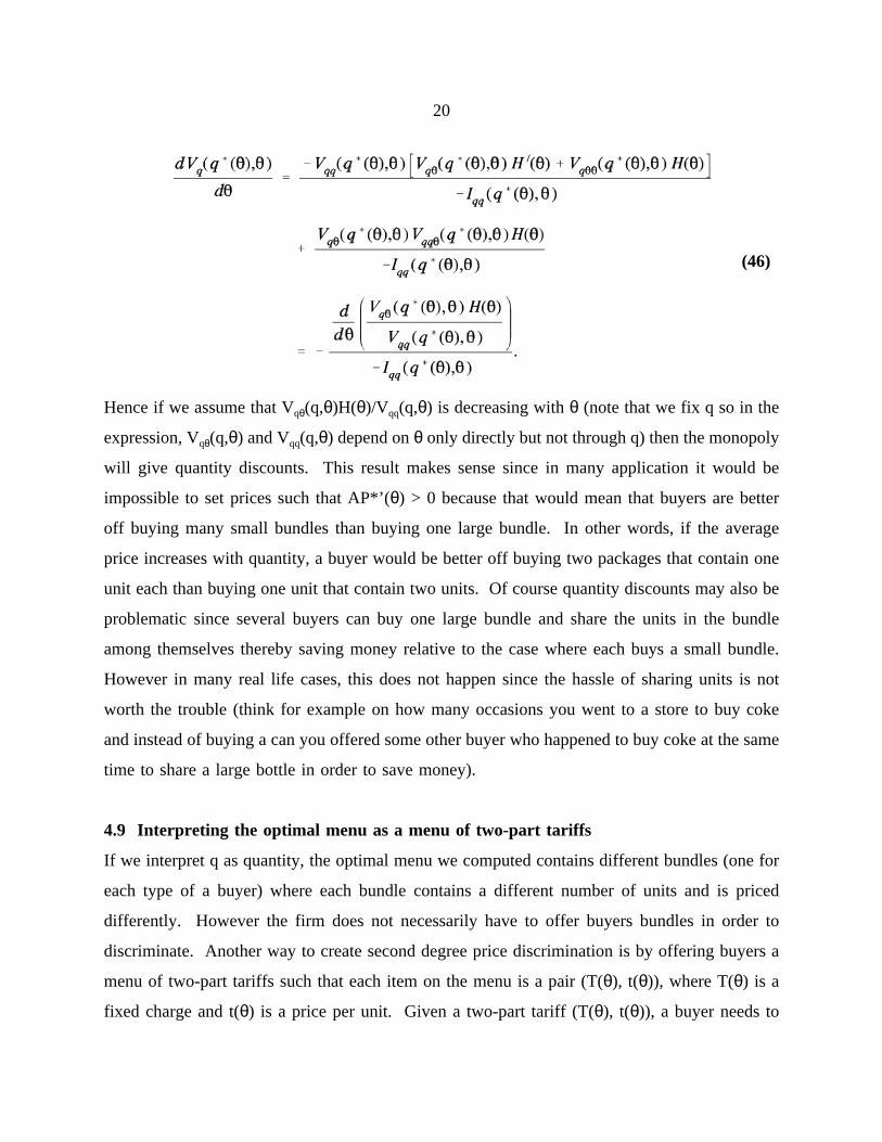
20

Hence if we assume that Vqθ(q,θ)H(θ)/Vqq(q,θ) is decreasing withθ (note that we fix q so in the

(46)

expression, Vqθ(q,θ) and Vqq(q,θ) depend onθ only directly but not through q) then the monopoly

will give quantity discounts. This result makes sense since in many application it would be

impossible to set prices such that AP*’(θ) > 0 because that would mean that buyers are better

off buying many small bundles than buying one large bundle. In other words, if the average

price increases with quantity, a buyer would be better off buying two packages that contain one

unit each than buying one unit that contain two units. Of course quantity discounts may also be

problematic since several buyers can buy one large bundle and share the units in the bundle

among themselves thereby saving money relative to the case where each buys a small bundle.

However in many real life cases, this does not happen since the hassle of sharing units is not

worth the trouble (think for example on how many occasions you went to a store to buy coke

and instead of buying a can you offered some other buyer who happened to buy coke at the same

time to share a large bottle in order to save money).

4.9 Interpreting the optimal menu as a menu of two-part tariffs

If we interpret q as quantity, the optimal menu we computed contains different bundles (one for

each type of a buyer) where each bundle contains a different number of units and is priced

differently. However the firm does not necessarily have to offer buyers bundles in order to

discriminate. Another way to create second degree price discrimination is by offering buyers a

menu of two-part tariffs such that each item on the menu is a pair (T(θ), t(θ)), where T(θ) is a

fixed charge and t(θ) is a price per unit. Given a two-part tariff (T(θ), t(θ)), a buyer needs to

21

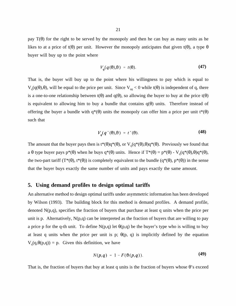
pay T(θ) for the right to be served by the monopoly and then he can buy as many units as he

likes to at a price of t(θ) per unit. However the monopoly anticipates that given t(θ), a typeθ

buyer will buy up to the point where

That is, the buyer will buy up to the point where his willingness to pay which is equal to

(47)

Vq(q(θ),θ), will be equal to the price per unit. Since Vqq < 0 while t(θ) is independent of q, there

is a one-to-one relationship between t(θ) and q(θ), so allowing the buyer to buy at the price t(θ)

is equivalent to allowing him to buy a bundle that contains q(θ) units. Therefore instead of

offering the buyer a bundle with q*(θ) units the monopoly can offer him a price per unit t*(θ)

such that

The amount that the buyer pays then is t*(θ)q*(θ), or Vq(q*(θ),θ)q*(θ). Previously we found that

(48)

a θ type buyer pays p*(θ) when he buys q*(θ) units. Hence if T*(θ) = p*(θ) - Vq(q*(θ),θ)q*(θ),

the two-part tariff (T*(θ), t*(θ)) is completely equivalent to the bundle (q*(θ), p*(θ)) in the sense

that the buyer buys exactly the same number of units and pays exactly the same amount.

5. Using demand profiles to design optimal tariffs

An alternative method to design optimal tariffs under asymmetric information has been developed

by Wilson (1993). The building block for this method is demand profiles. A demand profile,

denoted N(p,q), specifies the fraction of buyers that purchase at least q units when the price per

unit is p. Alternatively, N(p,q) can be interpreted as the fraction of buyers that are willing to pay

a price p for the q-th unit. To define N(p,q) letθ(p,q) be the buyer’s type who is willing to buy

at least q units when the price per unit is p;θ(p, q) is implicitly defined by the equation

Vq(q,θ(p,q)) = p. Given this definition, we have

That is, the fraction of buyers that buy at least q units is the fraction of buyers whoseθ’s exceed

(49)

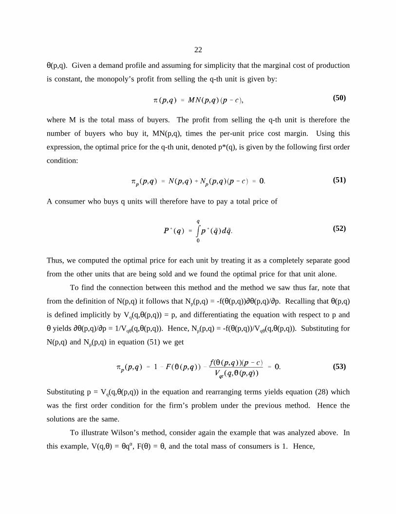
22

θ(p,q). Given a demand profile and assuming for simplicity that the marginal cost of production

is constant, the monopoly’s profit from selling the q-th unit is given by:

where M is the total mass of buyers. The profit from selling the q-th unit is therefore the

(50)

number of buyers who buy it, MN(p,q), times the per-unit price cost margin. Using this

expression, the optimal price for the q-th unit, denoted p*(q), is given by the following first order

condition:

A consumer who buys q units will therefore have to pay a total price of

(51)

Thus, we computed the optimal price for each unit by treating it as a completely separate good

(52)

from the other units that are being sold and we found the optimal price for that unit alone.

To find the connection between this method and the method we saw thus far, note that

from the definition of N(p,q) it follows that Np(p,q) = -f(θ(p,q))∂θ(p,q)/∂p. Recalling thatθ(p,q)

is defined implicitly by Vq(q,θ(p,q)) = p, and differentiating the equation with respect to p and

θ yields∂θ(p,q)/∂p = 1/Vqθ(q,θ(p,q)). Hence, Np(p,q) = -f(θ(p,q))/Vqθ(q,θ(p,q)). Substituting for

N(p,q) and Np(p,q) in equation (51) we get

Substituting p = Vq(q,θ(p,q)) in the equation and rearranging terms yields equation (28) which

(53)

was the first order condition for the firm’s problem under the previous method. Hence the

solutions are the same.

To illustrate Wilson’s method, consider again the example that was analyzed above. In

this example, V(q,θ) = θqα, F(θ) = θ, and the total mass of consumers is 1. Hence,

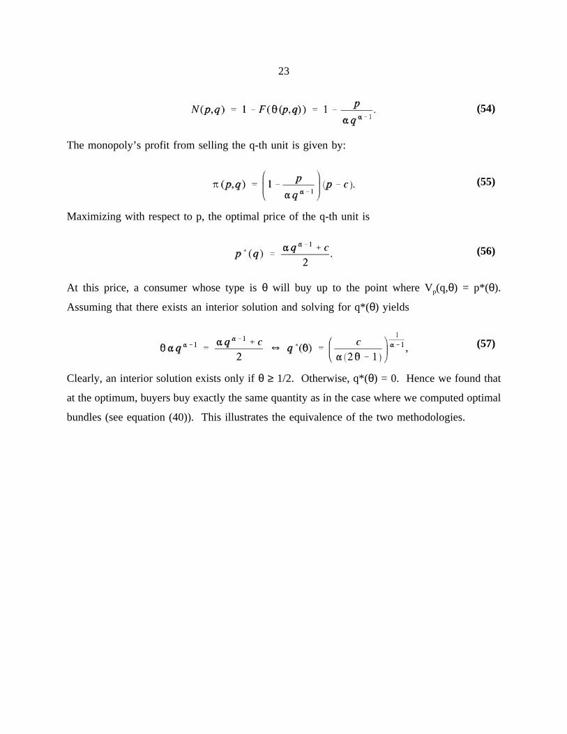
23

The monopoly’s profit from selling the q-th unit is given by:

(54)

Maximizing with respect to p, the optimal price of the q-th unit is

(55)

At this price, a consumer whose type isθ will buy up to the point where Vp(q,θ) = p*(θ).

(56)

Assuming that there exists an interior solution and solving for q*(θ) yields

Clearly, an interior solution exists only ifθ ≥ 1/2. Otherwise, q*(θ) = 0. Hence we found that

(57)

at the optimum, buyers buy exactly the same quantity as in the case where we computed optimal

bundles (see equation (40)). This illustrates the equivalence of the two methodologies.

24

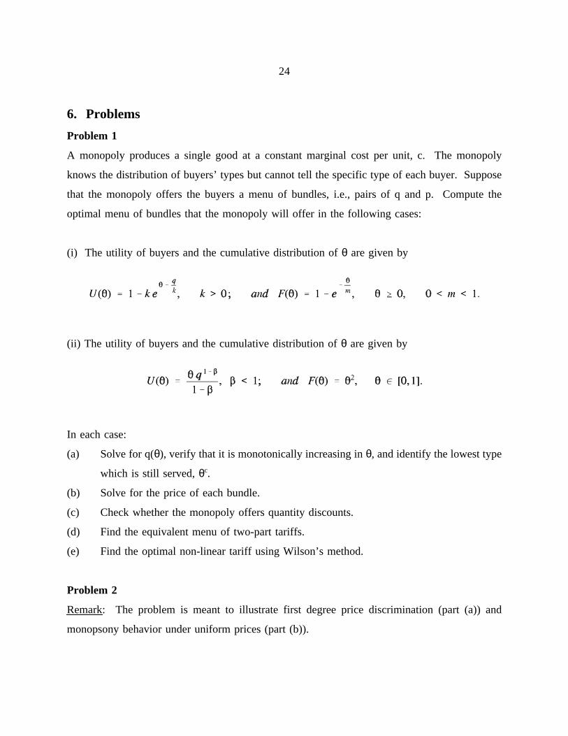
6. Problems

Problem 1

A monopoly produces a single good at a constant marginal cost per unit, c. The monopoly

knows the distribution of buyers’ types but cannot tell the specific type of each buyer. Suppose

that the monopoly offers the buyers a menu of bundles, i.e., pairs of q and p. Compute the

optimal menu of bundles that the monopoly will offer in the following cases:

(i) The utility of buyers and the cumulative distribution ofθ are given by

(ii) The utility of buyers and the cumulative distribution ofθ are given by

In each case:

(a) Solve for q(θ), verify that it is monotonically increasing inθ, and identify the lowest type

which is still served,θc.

(b) Solve for the price of each bundle.

(c) Check whether the monopoly offers quantity discounts.

(d) Find the equivalent menu of two-part tariffs.

(e) Find the optimal non-linear tariff using Wilson’s method.

Problem 2

Remark: The problem is meant to illustrate first degree price discrimination (part (a)) and

monopsony behavior under uniform prices (part (b)).

25

A monopoly sells a homogenous good. The inverse demand function for the good is p = 1-q,

where p denotes the price and q denotes the quantity that the monopoly sells (the monopoly

cannot use price discrimination on the market - all units must be sold at the same price). The

monopoly buys the good from a single manufacturer whose cost per unit is c < 1. The sequence

of events is as follows: the monopoly first offers the manufacturer to buy from him q units and

offers him in return a payment T. If the manufacturer accepts the offer, the monopoly takes the

q units and sells them on the market. If the manufacturer rejects the offer there is no trade and

all parties get a zero payoff.

(a) Suppose that the monopoly knows c. How many units will the monopoly buy from the

manufacturer and how much will he pay him? Compute the profits of the monopoly and

the manufacturer.

(b) Now suppose that the monopoly does not know c but knows that it is drawn from a

uniform distribution on the interval [0, 1]. How many units will the monopoly buy from

the manufacturer now and how much will he pay him? Compute the expected profit of

the monopoly and the ex ante expected profit of the manufacturer’s (by ex ante I mean

before the manufacturer knows his type; hence the expectation is taken on all possible

types).

26

References

Baron D. (1989), "Design of Regulatory Mechanisms and Institutions," inThe Handbook of

Industrial Organization, R. Schmalansee and R. Willig (eds.), Volume II, Chapter 24,

1347-1447, Elsevier Science Publishers B.V. (North Holland).

Baron D. and Myerson R. (1982), "Regulating a Monopolist with Unknown Costs,"

Econometrica,50: 911-930.

Maskin E., and Riley J. (1984), "Monopoly with Incomplete Information,"Rand Journal of

Economics,15: 171-196.

Mirrlees J. (1971), "An Exploration in the Theory of Optimal Taxation,"Review of Economic

Studies," 38: 175-208.

Mussa M. and Rosen S. (1978), "Monopoly and Product Quality,"Journal of Economic Theory,

18: 301-317.

Wilson R. (1993),Nonlinear Pricing, Oxford University Press.