Embed Size (px)
Citation preview
SECED NEWSLETTER - DECEMBER 2001 - Page 1
ISSN 0967-859X THE SOCIETY FOR EARTHQUAKE AND CIVIL
ENGINEERING DYNAMICS
NEWSLETTER
Volume 14 No 4 December 2001
Seismic Effects On Buried Structures David Smith of Scott Wilson Kirkpatrick & Co Ltd outlines the objectives of a seminar, which was SECED’s first meeting on the subject of seismic effects on buried structures. The seminar was an opportunity for the work of John Haines, Martin Morris and Ian Troman to be introduced to the Society. The seminar was a half-day meeting held at the ICE on 29th November 2000. Disruptions on the day caused by the railways created difficulties for some of the speakers, so to avoid curtailment of the presentations, the discussion at the end of the day was omitted and questions were submitted by Email. These are included as appropriate in the papers below. Richard Lunniss (Symonds Group) had to withdraw at the last moment so the presentation on submerged tunnels was made by Martin Morris of Hyder.
The topics identified for inclusion were: • Overview of damage to
underground structures. • Tunnels • Pipelines • Underground motion and variation
with depth • Caverns • Geotechnical and geophysical
information needed for the analysis
Underground we have both linear structures and caverns. Linear structures include tunnels for conveyance of people and liquids, pipelines and shafts. Caverns are mainly for storage of nuclear waste, water petroleum and liquefied gas, but they also contain power plants, military installations and even conference centres.
Categorised by means of construction, tunnels, the predominant form of underground structures in most countries, include immersed tube,
cut-and-cover and rock tunnels, whereas caverns are either cut-and-cover or in rock. This seminar considered sufficient of these to provide most of with a new and interesting perspective on ground/structure interaction.
Amongst these papers is new information, older information not previously published, simplified methods and rules of thumb to assess when no special measures, either in design or in construction, are likely to be required.
The seminar was inspired by the URS/JA Blume report of 1980 on ‘Earthquake Engineering of Large Underground Structures’, which is still
the only comprehensive study on the subject.
In acknowledgement of the fact that the deeper buried structures have performed generally better than surface structures, the speakers were asked, where possible, to identify particular forms of construction or details which were damage prone and so should be avoided. This was the common theme throughout the presentations and, being particularly relevant, is reflected in the recorded versions in this Special Edition of the Newsletter.
S E
S E C E D E D
SECED NEWSLETTER - DECEMBER 2001 - Page 2
0
0.1
0.2
0.3
0.4
0.5
0.6
0.7
0.8
0.9
Pea
k G
rou
nd
Acc
eler
atio
n (g
)
The observed damage to buried structures Tim Allmark of EQE International discusses damage to buried structures, illustrated by examples from the EQE database, and indicates how the knowledge can be applied. INTRODUCTION There is a wealth of experience data available to the engineer faced with the problem of assessing existing buried structures. For those undertaking design, the information is equally valuable as a guide towards the key features that should be considered. It encourages a necessary overview of the performance of the whole facility, resulting in a holistic approach to design and construction or assessment that ensures the “function” of the facility is to be maintained. This is illustrated by examples from earthquakes over the past 100 years.
TUNNELS A review of the past performance of a large number of underground openings during earthquakes was conducted by URS John Blume in 1980. The review indicated that underground structures in general are less severely affected than surface structures at the same geographic location. While a surface structure responds as a resonating cantilevered beam, amplifying the ground motion, an underground structure responds essentially with the ground. However, the review showed that severe damage is often associated with tunnels in soil and poor rock, whereas damage to tunnels in competent rock is usually (but not always) minor.
Peak ground motion parameters, can be extracted from the data to provide a broad synopsis of the performance, as can be seen in Figure 1.
Earthquake damage to underground structures may be attributed to the following key effects:
1. Fault crossing the line of the tunnels
2. Slope failure causing damage to the portal, or in some cases to shallow depth tunnels
3. Poor geological conditions adjacent to the tunnel leading to local/global instabilities
4. Long term degradation leaving tunnels in a weakened state
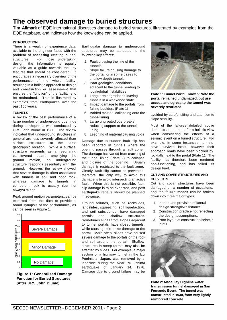
5. Impact damage to the portals from falling boulders (Plate 1)
6. Voided material collapsing onto the tunnel lining
7. Large ungrouted overbreaks reducing support to the tunnel lining
8. Leeching of material causing voids
Damage due to sudden fault slip has been reported in tunnels where the opening passes through a fault zone. The damage has varied from cracking of the tunnel lining (Plate 2) to collapse and closure of the opening. Usually damage is restricted to the fault zone. Clearly, fault slip cannot be prevented; therefore, the only way to avoid this damage is to avoid intersecting an active fault. When this is not possible, fault slip damage is to be expected, and post earthquake repairs should be planned in advance.
Ground failures, such as rockslides, landslides, squeezing, soil liquefaction, and soil subsidence, have damaged portals and shallow structures. Sometimes slides from slopes adjacent to tunnel portals have closed tunnels, while causing little or no damage to the portal. More often, slides have caused severe damage to the portals or the rock and soil around the portal. Shallow structures in steep terrain may also be affected by slides. For example, a major section of a highway tunnel in the Izu Peninsula, Japan, was removed by a landslide during the Near Izu-Oshima earthquake of January 14, 1978. Damage due to ground failure may be
avoided by careful siting and attention to slope stability.
Most of the failures detailed above demonstrate the need for a holistic view when considering the effects of a seismic event on a buried structure. For example, in some instances, tunnels have survived intact, however their approach roads have been blocked by rockfalls next to the portal (Plate 1). The facility has therefore been rendered non-functioning, and has failed its design brief.
CUT AND COVER STRUCTURES AND CULVERTS Cut and cover structures have been damaged on a number of occasions, and the failure modes can be broken down into three major types.
1. Inadequate provision of lateral design strength/resistance.
2. Construction practice not reflecting the design assumptions.
3. Poor layout of construction/seismic joints.
Plate 1: Tunnel Portal, Taiwan: Note the portal remained undamaged, but use access and egress to the tunnel was severely restricted.
Plate 2: Macaulay Highline water transmission tunnel damaged in San Fernando Event. The tunnel was constructed in 1930, from very lightly reinforced concrete
Figure 1: Generalised Damage Function for Buried Structures (After URS John Blume)
Severe Damage
Minor Damage
No Damage
SECED NEWSLETTER - DECEMBER 2001 - Page 3
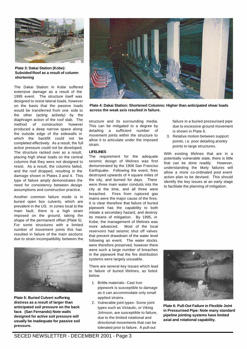
The Dakai Station in Kobe suffered extensive damage as a result of the 1995 event. The structure itself was designed to resist lateral loads, however on the basis that the passive loads would be transferred from one side to the other (acting actively) by the diaphragm action of the roof slab. The method of construction however produced a deep narrow space along the outside edge of the sidewalls in which the backfill could not be completed effectively. As a result, the full active pressure could not be developed. The structure racked over as a result, placing high shear loads on the central columns that they were not designed to resist. As a result, the columns failed, and the roof dropped, resulting in the damage shown in Plates 3 and 4. This type of failure amply demonstrates the need for consistency between design assumptions and construction practice.
Another common failure mode is in buried open box culverts, which are prevalent in the US. In zones local to the main fault, there is a high strain imposed on the ground, taking the shape of the permanent offset (Plate 5). For some structures with a limited number of movement joints this has resulted in failure of the main sections due to strain incompatibility between the
structure and its surrounding media. This can be mitigated to a degree by detailing a sufficient number of movement joints within the structure to allow it to articulate under the imposed strain.
LIFELINES The requirement for the adequate seismic design of lifelines was first demonstrated by the 1906 San Franciso Earthquake. Following the event, fires destroyed upwards of 4 square miles of the city, and burned for days. There were three main water conduits into the city at the time, and all three were breached. Fires from ruptured gas mains were the major cause of the fires. It is clear therefore that failure of buried pipework has the capability to both initiate a secondary hazard, and destroy its means of mitigation. By 1995, in Kobe, the management of lifelines was more advanced. Most of the local reservoirs had seismic shut off valves that prevent drawdown of the water level following an event. The water stocks were therefore preserved, however there were such a large number of breaches in the pipework that the fire distribution systems were largely unusable.
There are several key issues which lead to failure of buried lifelines, as listed below.
1. Brittle materials- Cast Iron pipework is susceptible to damage as it can accommodate only small applied strains.
2. Vulnerable joint types- Some joint types such as Victaulic, or Viking Johnson, are susceptible to failure, due to the limited rotational and directional movements that can be tolerated prior to failure. A pull-out
failure in a buried pressurised pipe due to excessive ground movement is shown in Plate 6.
3. Relative motion between support points, i.e. poor detailing at entry points to large structures.
With existing lifelines that are in a potentially vulnerable state, there is little that can be done readily. However, understanding the likely failures will allow a more co-ordinated post event action plan to be devised. This should identify the key issues at an early stage to facilitate the planning of mitigation.
Plate 3: Dakai Station (Kobe): Subsided Roof as a result of column shortening
Plate 4: Dakai Station: Shortened Columns: Higher than anticipated shear loads across the weak axis resulted in failure.
Plate 5: Buried Culvert suffering distress as a result of larger than anticipated soil pressure on the back face. (San Fernando) Note walls designed for active soil pressure will usually be inadequate for passive soil pressure.
Plate 6: Pull-Out Failure in Flexible Joint in Pressurised Pipe: Note many standard pipeline jointing systems have limited axial and rotational capability.
SECED NEWSLETTER - DECEMBER 2001 - Page 4
Seismic Effects on Immersed Tube Tunnels Martin Morris, Technical Director, Hyder Consulting Limited, briefly reviews the origins and evolution of immersed tube tunnels, their construction and their merits relative to bridges. He discusses the effects of earthquakes and how they can be reduced by the appropriate choice of bedding layer and joints, the impairment of the waterproofing and the problem of repair. He compares the free-field motion with that of a Flush analysis. INTRODUCTION Immersed tube tunnels are an increasingly popular means of crossing inland and nearshore waterways for road and rail projects. The technique may be said to have originated in USA and was developed into its modern European form in Holland from just before World War II. As always, the story is not quite so simple and there have been independent developments of the technique in Japan, USA and Hong Kong. Even the origins might actually said to be British since two engineers published experiments with cylinders in the River Thames in the 19th Century but their foresight exceeded the capacity of their available materials i.e. bricks.
The application of seismic effects to immersed tube tunnels takes, as usual, two forms: those of faulting and shaking. Faulting, involving major ground displacements or liquefaction, might well sensibly preclude immersed tube tunnel construction in the first place but the same might be said for any form of construction. Faulting damage will be very localised and provision can be made for local damage repair.
Shaking imposes arbitrary deformations on the tunnel structure: design takes the form of ensuring sufficient ductility to absorb the imposed deformations whilst retaining the capacity to carry static loads. The immersed tube tunnel
technique has some particular in built ductility as will be seen.
This paper begins with a short description of the immersed tube tunnelling technique for those not familiar with it. It then reviews seismic effects on these tunnels and then looks at methods of mitigation.
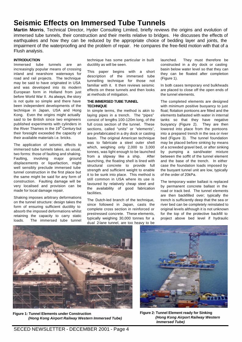
THE IMMERSED TUBE TUNNEL TECHNIQUE In simple terms, the method is akin to laying pipes in a trench. The “pipes” consist of lengths 100-120m long, of the full cross section of the tunnel. These sections, called “units” or “elements”, are prefabricated in a dry dock or casting basin. The original American technique was to fabricate a steel outer shell which, weighing only 2,000 to 3,000 tonnes, was light enough to be launched from a slipway like a ship. After launching, the floating shell is lined with structural concrete to provide full strength and sufficient weight to enable it to be sunk into place. This method is still common in USA where its use is favoured by relatively cheap steel and the availability of good fabrication facilities.
The Dutch-led branch of the technique, since followed in Japan, casts the complete cross section in reinforced or prestressed concrete. These elements, typically weighing 30,000 tonnes for a dual 2-lane tunnel, are too heavy to be
launched. They must therefore be constructed in a dry dock or casting basin below water level so that they can they can be floated after completion (Figure 1).
In both cases temporary end bulkheads are placed to close off the open ends of the tunnel elements.
The completed elements are designed with minimum positive buoyancy to just float; flotation pontoons are fitted and the elements ballasted with water in internal tanks so that they have negative buoyancy (Figure 2). They are then lowered into place from the pontoons into a prepared trench in the sea or river bed (Figure 3). The tunnel foundation may be placed before sinking by means of a screeded gravel bed, or after sinking by pumping a sand/water mixture between the soffit of the tunnel element and the base of the trench. In either case the foundation loads imposed by the buoyant tunnel unit are low, typically of the order of 20kPa.
The temporary water ballast is replaced by permanent concrete ballast in the road or track bed. The tunnel elements are then backfilled over; typically the trench is sufficiently deep that the sea or river bed can be completely reinstated to original levels although it is not unknown for the top of the protective backfill to project above bed level if hydraulic
Figure 1: Tunnel Elements under Construction (Hong Kong Airport Railway Western Immersed Tube)
Figure 2: Tunnel Element ready for Sinking (Hong Kong Airport Railway Western Immersed Tube)
SECED NEWSLETTER - DECEMBER 2001 - Page 5
conditions permit.
In early USA steel shell tunnels, the joints between tunnel elements were achieved by welding the steel shell. Most modern tunnels make use of a hydraulic jointing technique. This relies on differential water pressure to compress a large section rubber gasket between specially fabricated face plates. This gasket (Figure 4), commonly referred to as a “Gina” gasket, remains flexible and is capable of absorbing some of the shaking movement.
The advantages of the immersed tube tunnel technique can be summarised as
Against a bridge • No visual impact; • No requirement for deep
foundations; • Improved vertical alignment since
navigational depth requirement for shipping to pass over a tunnel is always less than the “airdraft” for vertical clearance.
Against a conventional driven tunnel • Improved vertical alignment since
the immersed tube element need only be 1-2m below the navigation envelope, whereas a driven tunnel must have a minimum cover for structural integrity (typically one
tunnel diameter); • Less dependence on ground
conditions. • Ability to tailor the cross section to fit
precisely to the project requirements. A circular or near circular driven tunnel may require additional bores to accommodate multi -lane or multi -track requirements.
Seismically, the flexibility of an immersed tube tunnel to move with the ground is advantageous, avoiding the amplification effects which may affect bridge structures, particularly those on the tall piers common in waterway crossings.
SEISMIC EFFECTS The primary seismic effects are summarised in Table 1.
Faulting may create major soil displacements in original ground, in foundation materials or in backfill. Such major displacements are typically very localised and provision can be made for damage repair. Where a sand foundation is used, its low density may make it prone to liquefaction. This can be locally strengthened e.g. by using sand/cement or bentonite cement, a topic discussed in more detail below under Special Issues.
When shaking occurs, transverse shear waves transmit the greatest proportion
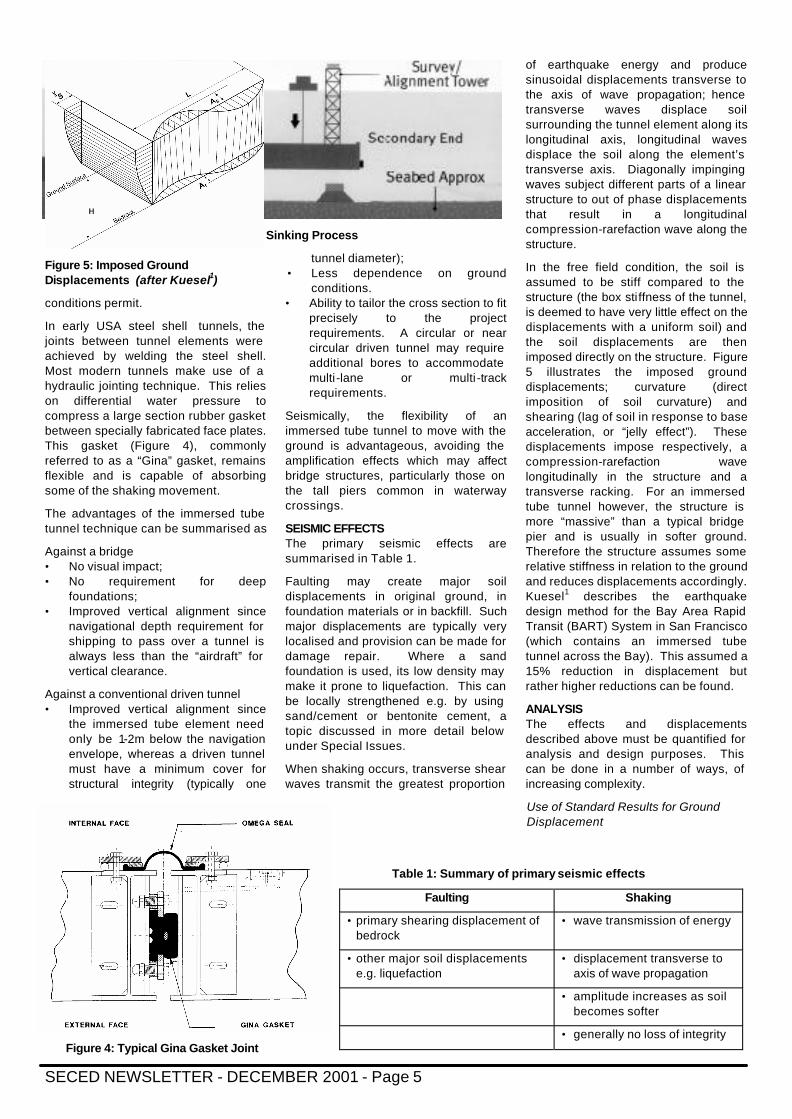
of earthquake energy and produce sinusoidal displacements transverse to the axis of wave propagation; hence transverse waves displace soil surrounding the tunnel element along its longitudinal axis, longitudinal waves displace the soil along the element’s transverse axis. Diagonally impinging waves subject different parts of a linear structure to out of phase displacements that result in a longitudinal compression-rarefaction wave along the structure.
In the free field condition, the soil is assumed to be stiff compared to the structure (the box sti ffness of the tunnel, is deemed to have very little effect on the displacements with a uniform soil) and the soil displacements are then imposed directly on the structure. Figure 5 illustrates the imposed ground displacements; curvature (direct imposition of soil curvature) and shearing (lag of soil in response to base acceleration, or “jelly effect”). These displacements impose respectively, a compression-rarefaction wave longitudinally in the structure and a transverse racking. For an immersed tube tunnel however, the structure is more “massive” than a typical bridge pier and is usually in softer ground. Therefore the structure assumes some relative stiffness in relation to the ground and reduces displacements accordingly. Kuesel1 describes the earthquake design method for the Bay Area Rapid Transit (BART) System in San Francisco (which contains an immersed tube tunnel across the Bay). This assumed a 15% reduction in displacement but rather higher reductions can be found.
ANALYSIS The effects and displacements described above must be quantified for analysis and design purposes. This can be done in a number of ways, of increasing complexity.
Use of Standard Results for Ground Displacement
Table 1: Summary of primary seismic effects
Faulting Shaking
• primary shearing displacement of bedrock
• wave transmission of energy
• other major soil displacements e.g. liquefaction
• displacement transverse to axis of wave propagation
• amplitude increases as soil becomes softer
• generally no loss of integrity
Figure 3: Immersed Tube Sinking Process
Figure 4: Typical Gina Gasket Joint
Figure 5: Imposed Ground Displacements (after Kuesel1)
SECED NEWSLETTER - DECEMBER 2001 - Page 6
In low risk areas, such as UK, Australia and Hong Kong, it has been traditional to either make no earthquake design provision or to rely on the use of static load coefficients to make a representation of the dynamic load. With increasing concern over the vulnerability of structures to earthquake (e.g. Australia has tightened its seismic design requirements and there is concern that earthquake risk in Hong Kong has been underestimated) there is a need for a more rational displacement related approach. The standard results developed by Kuesel1 for BART are based on the El Centro 1940 earthquake spectrum, often quoted as typical of a moderate shallow depth earthquake. This provides a transverse ground displacement spectrum based on a design earthquake of 0.33g in rock and shallow overburden (depth <21.3m above bedrock). From this it is possible to derive rational values for curvature and shearing displacement within appropriate limits of use.
The maximum strain in the structure due to curvature distortion is calculated from the critical wavelength (taken as 6 times the width of the structure in the plane of bending) and the corresponding amplitude taken from the ground displacement spectrum. For the BART Tunnel, this maximum strain was found to occur when the shear wave travelled obliquely to the structure, at an angle of 32°. If the strain is <0.0001, distortion is assumed to be elastic and no further provision need be made. If >0.0001, transverse articulation is required. Kuesel’s approach of course was for any underground railway structure; an immersed tube tunnel has this transverse articulation “built in” but the
effect of the elastic shortening on the joint has to be checked.
The shearing distortion (transverse displacement) is estimated from the depth of overburden above bedrock and the velocity of wave propagation through that overburden. Kuesel also gives an empirical formula for estimating the elastic distortion capacity of the structure. Alternatively the displacement induced imposed loading can be determined from a simple transverse plane frame model.
The simplicity of this empirical approach should not detract from its value; in Kuesel’s own words “…mathematical elaboration of this complex subject does not necessarily lead to an increased understanding of its nature….”
The use of an earthquake of this magnitude will be conservative for most areas of low seismic activity. Typically, the longitudinal wave will create displacements up to +/- 10mm over a 100m long element, which can be absorbed within the Gina gasket at each element-to-element joint. The joint will neither fail in compression nor open up under tension. Similarly, it will be found that the shearing distortion (transverse displacement) of the structure is within its ductile capacity.
Site Specific Ground Displacement Analysis For higher risk areas, a site-specific displacement analysis such as SHAKE can be undertaken. This determines sub surface accelerations and displacements in a single dimension which are therefore applicable on all
axes. Programs such as FLUSH employ finite element analysis to take soil-structure interaction, and hence structure stiffness, into account.
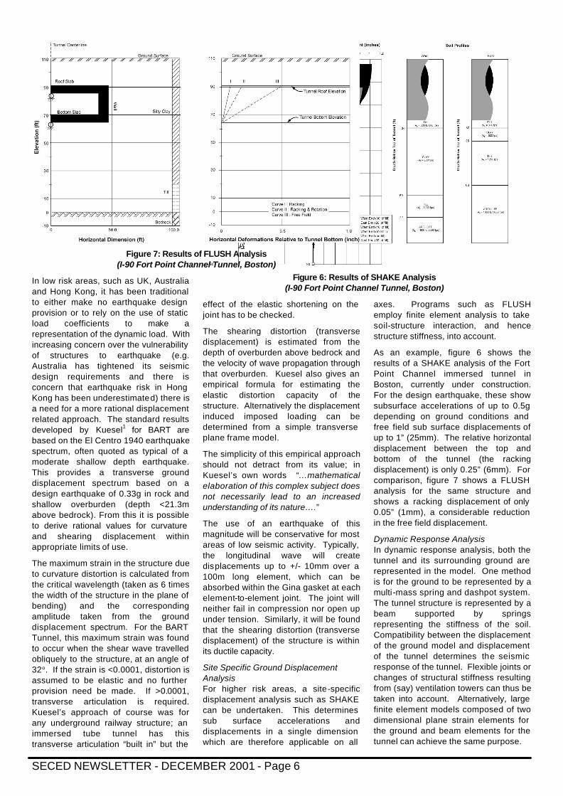
As an example, figure 6 shows the results of a SHAKE analysis of the Fort Point Channel immersed tunnel in Boston, currently under construction. For the design earthquake, these show subsurface accelerations of up to 0.5g depending on ground conditions and free field sub surface displacements of up to 1” (25mm). The relative horizontal displacement between the top and bottom of the tunnel (the racking displacement) is only 0.25” (6mm). For comparison, figure 7 shows a FLUSH analysis for the same structure and shows a racking displacement of only 0.05” (1mm), a considerable reduction in the free field displacement.
Dynamic Response Analysis In dynamic response analysis, both the tunnel and its surrounding ground are represented in the model. One method is for the ground to be represented by a multi -mass spring and dashpot system. The tunnel structure is represented by a beam supported by springs representing the stiffness of the soil. Compatibility between the displacement of the ground model and displacement of the tunnel determines the seismic response of the tunnel. Flexible joints or changes of structural stiffness resulting from (say) ventilation towers can thus be taken into account. Alternatively, large finite element models composed of two dimensional plane strain elements for the ground and beam elements for the tunnel can achieve the same purpose.
Figure 6: Results of SHAKE Analysis (I-90 Fort Point Channel Tunnel, Boston)
Figure 7: Results of FLUSH Analysis (I-90 Fort Point Channel Tunnel, Boston)
SECED NEWSLETTER - DECEMBER 2001 - Page 7
Ojiyama2 presents a useful summary of Japanese practice in seismic modelling of immersed tube tunnels . Ref 3 describes the application of dynamic response analysis to the Tama River Tunnel on the Expressway Bay Shore Route in Tokyo. The results in Table 2 taken from that paper illustrate the benefits of the flexible joint in reducing earthquake forces.
It can be seen that, as might be expected, the flexible (i.e. Gina) joint reduces the forces on the tunnel significantly. However, it can also be seen that in a high seismicity area such as Tokyo, potential displacements are of the order of 90mm, much greater than the values of 10mm or so in low risk areas. These movements cannot be accommodated by the Gina gasket without opening the joint. A common method of preventing this is to tie the joint using prestressing cables (refer Special issues below).
Such complex analysis is only appropriate to very high risk areas e.g. Japan, or very complex structures or major changes of cross section in medium risk areas.
DESIGN CRITERIA The curvature distortion creates longitudinal strain in the structure. This
strain, added to any conventional bending strain must remain within the elastic range. The strain applied to the length of an immersed tube element will create a lengthening and shortening of the element that must be absorbed in the Gina gasket. Typically the change in length will be of the order of 10mm. The gasket is approximately 200mm thick in its uncompressed form and is compressed in the joint to about 120mm. The compression of 80mm has to cater for age-related relaxation, relative settlement of the tunnel units with time etc. However, longitudinal movements of this order can generally be accommodated.
Racking of the structure as a result of the design earthquake must stay within the elastic distortion capacity. In areas of low seismic risk, the distortion capacity will normally be deemed sufficient if the structure is designed and detailed in accordance with national codes as a ductile structure. Alternatively the distortion capacity of the cross section can be calculated. This will ensure that the structure remains elastic with no cracking. The leakage threshold for a reinforced concrete tunnel would be the point where cracks did not close after racking displacement. If the earthquake exceeds the design
earthquake the structure must still avoid collapse, even if significant damage occurs. Here, ductile detailing will ensure the integrity of the main reinforcement and prevent actual collapse. Immersed tube tunnels by their nature are subject to high hydrostatic loading, which will generally require the use of substantial shear reinforcement in the structural sections. In areas of high seismicity, this will require review to ensure that it meets the requirements of ductile detailing in the earthquake sense; this may sometimes require the addition of diagonal bars tying-in the outer tensile reinforcement in the corners of the section.
SPECIAL ISSUES FOR IMMERSED TUBE TUNNELS
Liquefaction The sand-placed foundation initially self-compacts and is further compacted on release of the tunnel element from its jacks. Accordingly, it is very loosely compacted and therefore prone to liquefaction in seismic conditions. Typically in earthquake areas, the sand can be replaced by bentonite cement or neat cement grout that is pre-mixed and pumped into place. A screeded gravel mattress as a foundation is less vulnerable to pore water pressure build-up and may be a cost-effective alternative to a sand foundation in seismic areas. However for wide road tunnels (say >30m) the screed may be difficult to place to the required tolerance (typically +/-50mm).
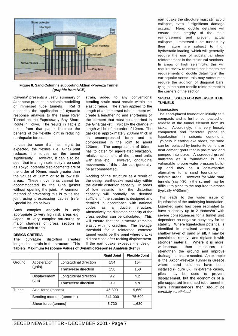
This leads to the wider issue of liquefaction of the underlying foundation. Liquefied sand has been estimated to have a density up to 2 tonnes/m3 with severe consequences for a tunnel unit dependent on negative buoyancy for its stability. Where liquefaction potential is identified in localised areas e.g. a shallow layer of sand or silt, it may be possible to remove and replace it with stronger material. Where it is more widespread, then measures to strengthen the ground and improve drainage paths are needed. An example is the Aktion-Preveza Tunnel in Greece where sand columns have been installed (Figure 8). In extreme cases, piles may be used to prevent displacement, but the economics of a pile-supported immersed tube tunnel in such circumstances then should be carefully scrutinised.
Table 2: Maximum Response Values of Dynamic Response Analysis (Ref 3)
Rigid Joint Flexible Joint
Longitudinal direction 154 154 Acceleration (gals)
Transverse direction 158 158
Longitudinal direction 9.2 9.2
Ground
Displacement (cm)
Transverse direction 9.9 9.9
Axial force (tonnes) 45,300 9,660
Bending moment (tonne-m) 341,000 75,600
Tunnel
Shear force (tonnes) 5,730 1,630
Figure 8: Sand Columns supporting Aktion -Preveza Tunnel (graphic from NCE)
SECED NEWSLETTER - DECEMBER 2001 - Page 8
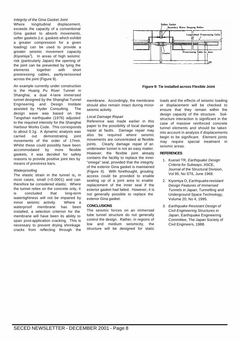
Integrity of the Gina Gasket Joint Where longitudinal displacement, exceeds the capacity of a conventional Gina gasket to absorb movements, softer gaskets (i.e. gaskets which exhibit a greater compression for a given loading) can be used to provide a greater seismic movement capacity (Kiyomiya2). In areas of high seismic risk (particularly Japan) the opening of the joint can be prevented by tying the elements together with short prestressing cables, partly-tensioned across the joint (Figure 9).
An example currently under construction is the Huang Pu River Tunnel in Shanghai, a dual 4-lane immersed tunnel designed by the Shanghai Tunnel Engineering and Design Institute assisted by Hyder Consulting. The design wave was based on the Tangshan earthquake (1976) adjusted to the required intensity for the Shanghai Harbour Works Code. This corresponds to about 0.1g. A dynamic analysis was carried out demonstrating joint movements of the order of 17mm. Whilst these could possibly have been accommodated by more flexible gaskets, it was decided for safety reasons to provide positive joint ties by means of prestress bars.
Waterproofing The elastic strain in the tunnel is , in most cases, small (<0.0001) and can therefore be considered elastic. Where the tunnel relies on the concrete only, it is concluded that long-term watertightness will not be impaired by minor seismic activity. Where a waterproof membrane has been installed, a selection criterion for the membrane will have been its ability to span post-application cracking. This is necessary to prevent drying shrinkage cracks from reflecting through the
membrane. Accordingly, the membrane should also remain intact during minor seismic activity.
Local Damage Repair Reference was made earlier in this paper to the possibility of local damage repair at faults. Damage repair may also be required where seismic movements are concentrated at flexible joints. Clearly damage repair of an underwater tunnel is not an easy matter. However, the flexible joint already contains the facility to replace the inner “omega” seal, provided that the integrity of the exterior Gina gasket is maintained (Figure 4). With forethought, grouting access could be provided to enable sealing up of a joint area to enable replacement of the inner seal if the exterior gasket had failed. However, it is not generally possible to replace the exterior Gina gasket.
CONCLUSIONS The seismic forces on an immersed tube tunnel structure do not generally control the design. Rather, in regions of low and medium seismicity, the structure will be designed for static
loads and the effects of seismic loading or displacement will be checked to ensure that they remain within the design capacity of the structure. Soil-structure interaction is significant in the case of massive reinforced concrete tunnel elements and should be taken into account in analysis if displacements begin to be significant. Element joints may require special treatment in seismic areas.
REFERENCES
1. Kuesel TR, Earthquake Design Criteria for Subways, ASCE, Journal of the Structural Division, Vol 95, No ST6, June 1969.
2. Kiyomiya O, Earthquake-resistant Design Features of Immersed Tunnels in Japan, Tunnelling and Underground Space Technology, Volume 20, No 4, 1995.
3. Earthquake Resistant Design of Civil Engineering Structures in Japan, Earthquake Engineering Committee, The Japan Society of Civil Engineers, 1988.
Figure 9: Tie installed across Flexible Joint
SECED NEWSLETTER - DECEMBER 2001 - Page 9
Design of Tunnels for Earthquake Ground Motions Colin Robertson, director of the Halcrow Group, outlines the various ways in which earthquakes affect tunnels and comments on the generally low vulnerability of tunnels to the effects of earthquakes. He reviews the relevant seismic waves and describes the design methods used in the USA and Japan and concludes with an example demonstrating how alterations in the construction can significantly improve the performance in earthquakes. INTRODUCTION In general terms underground structures are less severely affected by earthquakes than above ground structures. There are two principal reasons for this. Firstly, below ground structures are designed for high levels of external load due to ground and water pressures. The increase in these loads due to seismic ground motions is often within the elastic capacity of the structures, after allowing for partial material and load factors. Secondly, the response of an above ground structure is controlled by resonance with the ground motion at the foundations, whilst that for a below ground structure is typically compliant with the ground motion itself. Resonance in free standing structures can induce loads and displacements much greater than those from the non-seismic combinations. This can lead to member rupture and instability, leading to failure of structures not designed for these effects. Conversely loads experienced by compliant structures in the ground during a seismic event are controlled by the ground strains and can typically be absorbed without the structures losing their ability to carry static loads.
Tunnels form a special sub-set of underground structures and are distinguished by their linear nature and relatively simple structural form. This contributes in part to their good seismic performance as well as simplifying their analysis and design.
Before initiating a design process, it is necessary to understand the modes of failure against which protection is to be provided. For tunnels, there are three different modes, these and the strategy for dealing with them are identified below:
• Fault slip - Design to avoid intersecting
active faults if this is possible. - Design to facilitate post-seismic
repairs, for example oversize tunnel in the fault zone so that some slip can be accommodated without the need for new excavations to realign the tunnel post-event.
• Ground Failure
- Tunnels can be badly affected by ground slips, landslides, subsidence and liquefaction.
- These failures can be reduced by careful siting and alignment of the tunnel, by appropriate geotechnical design to give stable slopes and actions such as ground improvement to minimise subsidence and liquefaction potential.
• Direct Effects of Ground Motions - The ground subjects the tunnel to
straining and inertial loading. - Simplified design approaches for
this mode are the subject of this paper.
American and Japanese procedures for hand analysis are outlined and a further simple procedure as adopted for a project in the UK is also given.
To enable effective design strategies to be adopted it is necessary to have an understanding of how the tunnel and ground interact during a seismic event.
GROUND MOTION CHARACTERISATION Seismic motions propagate through the ground in a variety of waveforms. These are:
Body Waves - Compression Waves (analogous to
sound), referred to as P waves. - Shear waves, referred to as SH or SV
waves depending on the direction of particle motion, which are
perpendicular to the direction of propagation.
Surface Waves - Rayleigh waves have particle
motions that form a vertical orbit in the plane containing the direction of wave propagation; they decay rapidly with depth and are analogous to sea waves.
- Love waves have a horizontal shear motion perpendicular to the direction of propagation, decay with depth and are found in soft deposits overlying rock.
The above description of the motion is sufficient to understand the following discussion.
TUNNEL-GROUND INTERACTION The ground motions can be conceptualised as a strain field propagating through the ground. A flexible tunnel will conform to the ground motion and experience equivalent strains. A stiff tunnel will resist deformation and will experience lower strains but higher imposed loads (Figures 1 & 2).
Studies in support of the San Francisco Bay Area Rapid Transport (SFBART) scheme in the late 1950s led to an appreciation of the manner in which tunnels and ground interact during a seismic event and generated a design process, which can be undertaken by
sinØ Ø)
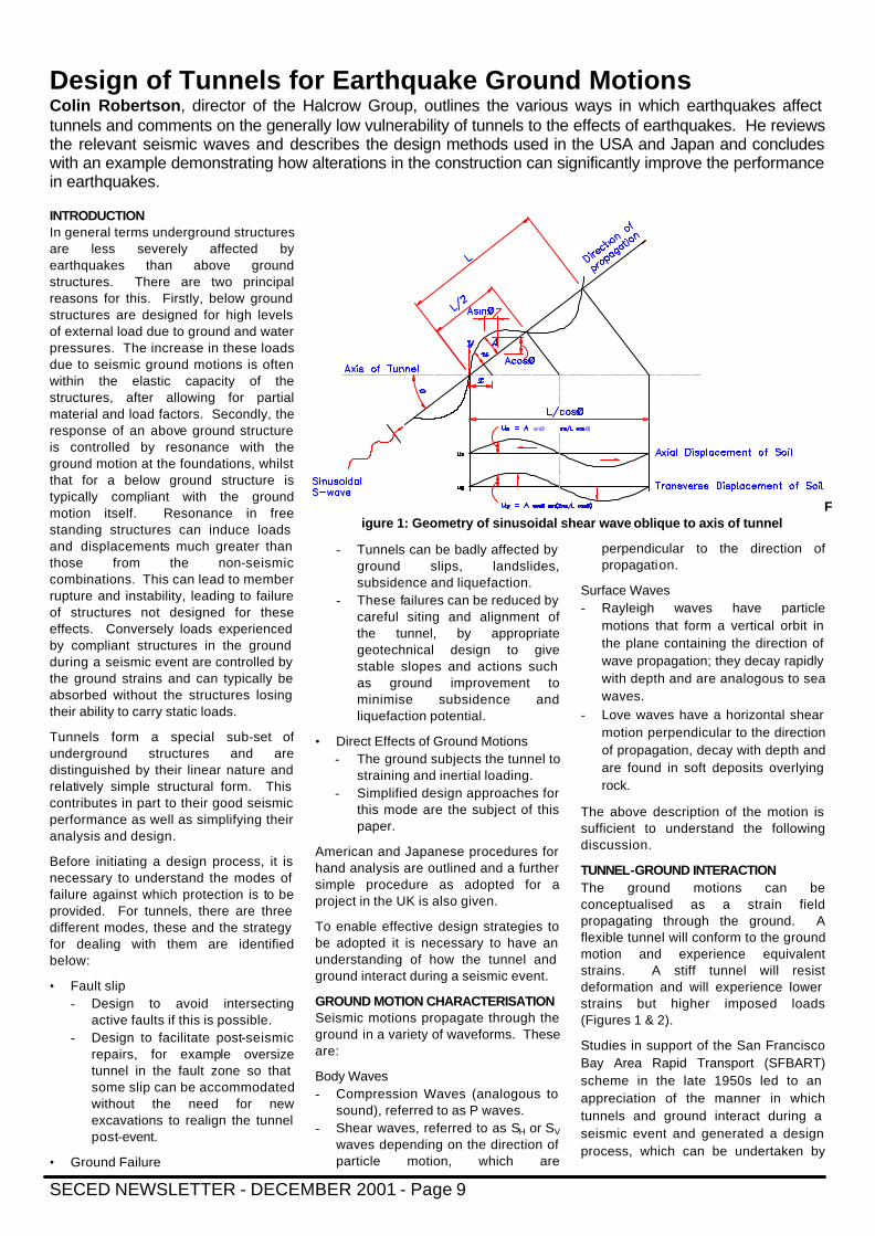
Figure 1: Geometry of sinusoidal shear wave oblique to axis of tunnel
SECED NEWSLETTER - DECEMBER 2001 - Page 10
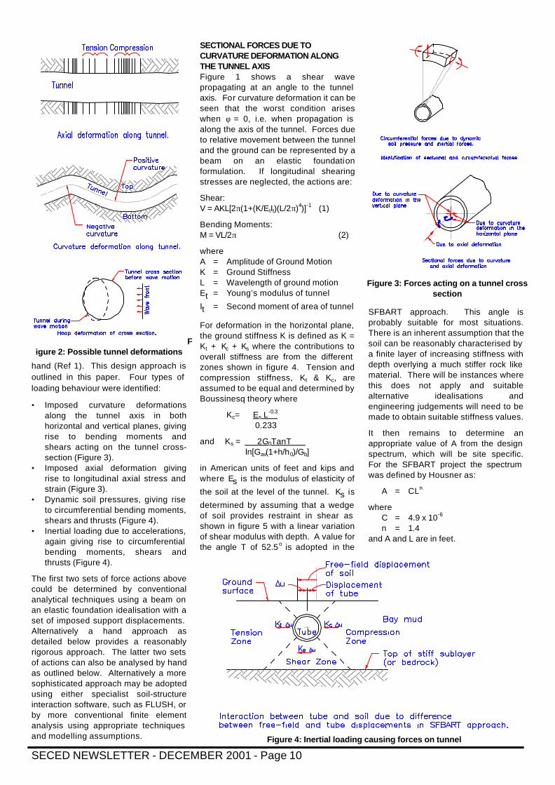
hand (Ref 1). This design approach is outlined in this paper. Four types of loading behaviour were identified:
• Imposed curvature deformations along the tunnel axis in both horizontal and vertical planes, giving rise to bending moments and shears acting on the tunnel cross-section (Figure 3).
• Imposed axial deformation giving rise to longitudinal axial stress and strain (Figure 3).
• Dynamic soil pressures, giving rise to circumferential bending moments, shears and thrusts (Figure 4).
• Inertial loading due to accelerations, again giving rise to circumferential bending moments, shears and thrusts (Figure 4).
The first two sets of force actions above could be determined by conventional analytical techniques using a beam on an elastic foundation idealisation with a set of imposed support displacements. Alternatively a hand approach as detailed below provides a reasonably rigorous approach. The latter two sets of actions can also be analysed by hand as outlined below. Alternatively a more sophisticated approach may be adopted using either specialist soil-structure interaction software, such as FLUSH, or by more conventional finite element analysis using appropriate techniques and modelling assumptions.
SECTIONAL FORCES DUE TO CURVATURE DEFORMATION ALONG THE TUNNEL AXIS Figure 1 shows a shear wave propagating at an angle to the tunnel axis. For curvature deformation it can be seen that the worst condition arises when φ = 0, i.e. when propagation is along the axis of the tunnel. Forces due to relative movement between the tunnel and the ground can be represented by a beam on an elastic foundation formulation. If longitudinal shearing stresses are neglected, the actions are:
Shear: V = AKL[2π(1+(K/EtIt)(L/2π)4)]-1 (1)
Bending Moments: M = VL/2π (2)
where A = Amplitude of Ground Motion K = Ground Stiffness L = Wavelength of ground motion Et = Young’s modulus of tunnel
It = Second moment of area of tunnel
For deformation in the horizontal plane, the ground stiffness K is defined as K = Kt + Kc + Ks where the contributions to overall stiffness are from the different zones shown in figure 4. Tension and compression stiffness, Kt & Kc, are assumed to be equal and determined by Boussinesq theory where
Kc= Es L-0.3
0.233
and Ks = 2G0TanT ln[Gav(1+h/h0)/Gb]
in American units of feet and kips and where Es is the modulus of elasticity of
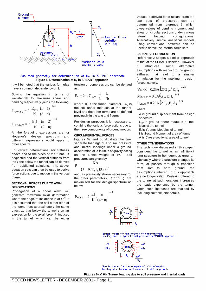
the soil at the level of the tunnel. Ks is
determined by assuming that a wedge of soil provides restraint in shear as shown in figure 5 with a linear variation of shear modulus with depth. A value for the angle T of 52.5o is adopted in the
SFBART approach. This angle is probably suitable for most situations. There is an inherent assumption that the soil can be reasonably characterised by a finite layer of increasing stiffness with depth overlying a much stiffer rock like material. There will be instances where this does not apply and suitable alternative idealisations and engineering judgements will need to be made to obtain suitable stiffness values.
It then remains to determine an appropriate value of A from the design spectrum, which will be site specific. For the SFBART project the spectrum was defined by Housner as:
A = CLn
where C = 4.9 x 10⁻⁶ n = 1.4
and A and L are in feet.
Figure 4: Inertial loading causing forces on tunnel
Figure 3: Forces acting on a tunnel cross
section
Figure 2: Possible tunnel deformations
SECED NEWSLETTER - DECEMBER 2001 - Page 11
It will be noted that the various formulae have a common dependency on L.
Solving the equation in terms of wavelength to maximise shear and bending respectively yields the following:
1/4tt
VMAX n)(31)(n.
KIE2L
−+=
1/4tt
MMAX n)(2)2(n
.K
IE2L
−+
=
All the foregoing expressions are for Housner’s design spectrum and different expressions would apply to other spectra.
For vertical deformations, soil stiffness above and to the sides of the tunnel is neglected and the vertical stiffness from the zone below the tunnel can be derived from published solutions. The above equation sets can then be used to derive force actions due to motion in the vertical plane.
SECTIONAL FORCES DUE TO AXIAL DEFORMATIONS Propagation of a shear wave will generate maximum axial deformation where the angle of incidence is at 45o. If it is assumed that the soil either side of the tunnel has approximately the same effect as that below the tunnel then an expression for the axial force, F, induced in the tunnel, which can be either
tension or compression, can be derived as:
+=2hL
LhG2dF AV0?
where do is the tunnel diameter, GAV is the soil shear modulus at the tunnel level and the other terms are as defined previously in the text and figures.
For design purposes it is necessary to combine the various force actions due to the three components of ground motion.
CIRCUMFERENTIAL FORCES Figures 6a and 6b illustrate the two separate loadings due to soil pressure and inertial loadings under a ground acceleration of a in units of gravity acting on the tunnel weight of W. Soil pressures are given by
4tt )(L/2)IK/E(1
KAP
+=
and, as previously shown necessary for the other parameters, Ph and Pv are maximised for the design spectrum as below
1/4
MAX n)(4n.
KEI2P
−
=
Values of derived force actions from the two sets of pressures can be determined from reference 6, which gives values of bending moment and shear on circular sections under various lateral loading configurations. Alternatively simple analytical models using conventional software can be used to derive the internal force sets.
JAPANESE FORMULATION Reference 2 adopts a similar approach to that of the SFBART scheme. However it introduces some alternative assumptions with respect to the ground stiffness that lead to a simpler formulation for the maximum design forces, namely.
( )0.25tt
3avMAX IE27G0.25AV =
( )0.5ttavMAX IEG0.5AM =
( )0.5ttavMAX AE2G0.25AP =
where
A is ground displacement from design spectrum Gav is ground shear modulus at the level of the tunnel Et is Youngs Modulus of tunnel It is Second Moment of area of tunnel At is Cross-sectional area of tunnel
OTHER CONSIDERATIONS The technique discussed in this paper considers the tunnel as an infinitely / long structure in homogenous ground. Obviously where a structure changes its form, or passes through a transition from soft to hard ground, the assumptions inherent in this approach are no longer valid. Restraint offered to the tunnel at such locations increases the loads experience by the tunnel. Often such increases are avoided by including suitable joint details.
Figures 6a & 6b: Tunnel loading due to soil pressure and inertial loads
Figure 5: Determination of Ks in SFBART approach
SECED NEWSLETTER - DECEMBER 2001 - Page 12
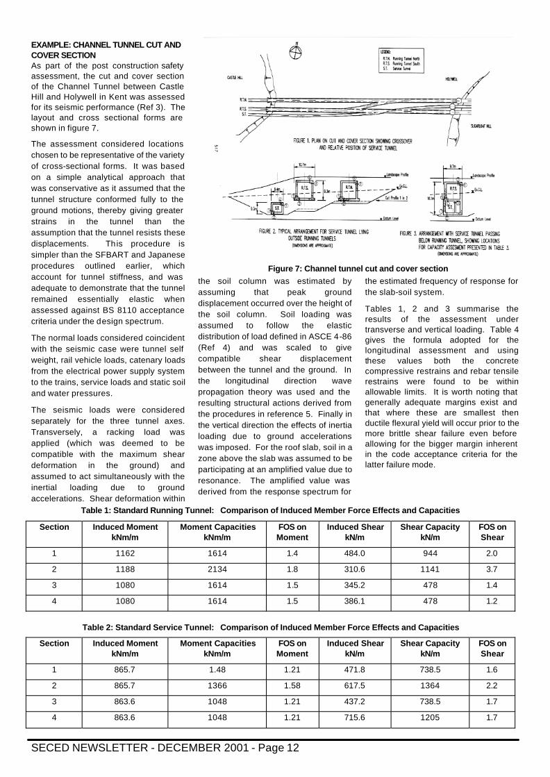
EXAMPLE: CHANNEL TUNNEL CUT AND COVER SECTION As part of the post construction safety assessment, the cut and cover section of the Channel Tunnel between Castle Hill and Holywell in Kent was assessed for its seismic performance (Ref 3). The layout and cross sectional forms are shown in figure 7.
The assessment considered locations chosen to be representative of the variety of cross-sectional forms. It was based on a simple analytical approach that was conservative as it assumed that the tunnel structure conformed fully to the ground motions, thereby giving greater strains in the tunnel than the assumption that the tunnel resists these displacements. This procedure is simpler than the SFBART and Japanese procedures outlined earlier, which account for tunnel stiffness, and was adequate to demonstrate that the tunnel remained essentially elastic when assessed against BS 8110 acceptance criteria under the design spectrum.
The normal loads considered coincident with the seismic case were tunnel self weight, rail vehicle loads, catenary loads from the electrical power supply system to the trains, service loads and static soil and water pressures.
The seismic loads were considered separately for the three tunnel axes. Transversely, a racking load was applied (which was deemed to be compatible with the maximum shear deformation in the ground) and assumed to act simultaneously with the inertial loading due to ground accelerations. Shear deformation within
the soil column was estimated by assuming that peak ground displacement occurred over the height of the soil column. Soil loading was assumed to follow the elastic distribution of load defined in ASCE 4-86 (Ref 4) and was scaled to give compatible shear displacement between the tunnel and the ground. In the longitudinal direction wave propagation theory was used and the resulting structural actions derived from the procedures in reference 5. Finally in the vertical direction the effects of inertia loading due to ground accelerations was imposed. For the roof slab, soil in a zone above the slab was assumed to be participating at an amplified value due to resonance. The amplified value was derived from the response spectrum for
the estimated frequency of response for the slab-soil system.
Tables 1, 2 and 3 summarise the results of the assessment under transverse and vertical loading. Table 4 gives the formula adopted for the longitudinal assessment and using these values both the concrete compressive restrains and rebar tensile restrains were found to be within allowable limits. It is worth noting that generally adequate margins exist and that where these are smallest then ductile flexural yield will occur prior to the more brittle shear failure even before allowing for the bigger margin inherent in the code acceptance criteria for the latter failure mode.
Figure 7: Channel tunnel cut and cover section
Table 1: Standard Running Tunnel: Comparison of Induced Member Force Effects and Capacities
Section Induced Moment kNm/m
Moment Capacities kNm/m
FOS on Moment
Induced Shear kN/m
Shear Capacity kN/m
FOS on Shear
1 1162 1614 1.4 484.0 944 2.0
2 1188 2134 1.8 310.6 1141 3.7
3 1080 1614 1.5 345.2 478 1.4
4 1080 1614 1.5 386.1 478 1.2
Table 2: Standard Service Tunnel: Comparison of Induced Member Force Effects and Capacities
Section Induced Moment kNm/m
Moment Capacities kNm/m
FOS on Moment
Induced Shear kN/m
Shear Capacity kN/m
FOS on Shear
1 865.7 1.48 1.21 471.8 738.5 1.6
2 865.7 1366 1.58 617.5 1364 2.2
3 863.6 1048 1.21 437.2 738.5 1.7
4 863.6 1048 1.21 715.6 1205 1.7
SECED NEWSLETTER - DECEMBER 2001 - Page 13
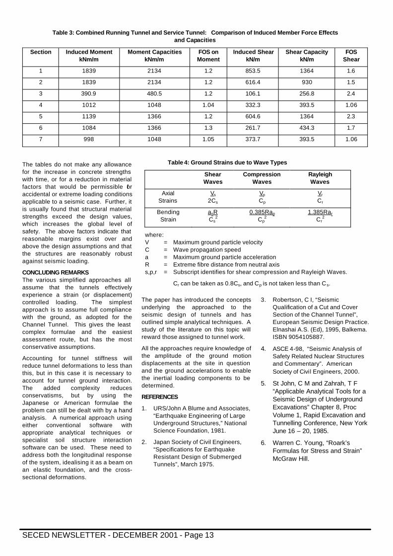
The tables do not make any allowance for the increase in concrete strengths with time, or for a reduction in material factors that would be permissible for accidental or extreme loading conditions applicable to a seismic case. Further, it is usually found that structural material strengths exceed the design values, which increases the global level of safety. The above factors indicate that reasonable margins exist over and above the design assumptions and that the structures are reasonably robust against seismic loading.
CONCLUDING REMARKS The various simplified approaches all assume that the tunnels effectively experience a strain (or displacement) controlled loading. The simplest approach is to assume full compliance with the ground, as adopted for the Channel Tunnel. This gives the least complex formulae and the easiest assessment route, but has the most conservative assumptions.
Accounting for tunnel stiffness will reduce tunnel deformations to less than this, but in this case it is necessary to account for tunnel ground interaction. The added complexity reduces conservatisms, but by using the Japanese or American formulae the problem can still be dealt with by a hand analysis. A numerical approach using either conventional software with appropriate analytical techniques or specialist soil structure interaction software can be used. These need to address both the longitudinal response of the system, idealising it as a beam on an elastic foundation, and the cross-sectional deformations.
The paper has introduced the concepts underlying the approached to the seismic design of tunnels and has outlined simple analytical techniques. A study of the literature on this topic will reward those assigned to tunnel work.
All the approaches require knowledge of the amplitude of the ground motion displacements at the site in question and the ground accelerations to enable the inertial loading components to be determined.
REFERENCES
1. URS/John A Blume and Associates, “Earthquake Engineering of Large Underground Structures,” National Science Foundation, 1981.
2. Japan Society of Civil Engineers, “Specifications for Earthquake Resistant Design of Submerged Tunnels”, March 1975.
3. Robertson, C I, “Seismic Qualification of a Cut and Cover Section of the Channel Tunnel”, European Seismic Design Practice. Elnashai A.S. (Ed), 1995, Balkema. ISBN 9054105887.
4. ASCE 4-98, “Seismic Analysis of Safety Related Nuclear Structures and Commentary”. American Society of Civil Engineers, 2000.
5. St John, C M and Zahrah, T F “Applicable Analytical Tools for a Seismic Design of Underground Excavations” Chapter 8, Proc Volume 1, Rapid Excavation and Tunnelling Conference, New York June 16 – 20, 1985.
6. Warren C. Young, “Roark’s Formulas for Stress and Strain” McGraw Hill.
Table 3: Combined Running Tunnel and Service Tunnel: Comparison of Induced Member Force Effects and Capacities
Section Induced Moment kNm/m
Moment Capacities kNm/m
FOS on Moment
Induced Shear kN/m
Shear Capacity kN/m
FOS Shear
1 1839 2134 1.2 853.5 1364 1.6
2 1839 2134 1.2 616.4 930 1.5
3 390.9 480.5 1.2 106.1 256.8 2.4
4 1012 1048 1.04 332.3 393.5 1.06
5 1139 1366 1.2 604.6 1364 2.3
6 1084 1366 1.3 261.7 434.3 1.7
7 998 1048 1.05 373.7 393.5 1.06
Table 4: Ground Strains due to Wave Types
Shear Waves
Compression Waves
Rayleigh Waves
Axial Strains
Vs
2Cs Vp
Cp Vr
Cr
Bending Strain
asR Cs
2 0.385Rap
Cp2
1.385Rar
Cr2
where: V = Maximum ground particle velocity C = Wave propagation speed a = Maximum ground particle acceleration R = Extreme fibre distance from neutral axis s,p,r = Subscript identifies for shear compression and Rayleigh Waves.
Cr can be taken as 0.8Cs, and Cp is not taken less than C s.
SECED NEWSLETTER - DECEMBER 2001 - Page 14
On Shaky Ground John Haines Reader of Geodesy and Geophysics in the Department of Earth Sciences, Bullard Laboratories, University of Cambridge discusses the prediction and predictability of earthquake ground motion and the effect of depth. A prerequisite to predicting ground motion in soil and rock is that spatial variation in ground motion can be attributed to geotechnical and geophysical phenomenon. The appreciation for the reasons for variation at the surface is an important factor in estimating the effects at depth.
Having had some previous success in modelling seismic wave propagation in complex situations, the then New Zealand Department of Scientific and Industrial Research (DSIR) at the end of the 1980s supported my exploration of the problem of predicting actual ground motion in earthquakes; in particular, in identifying the effects of surface topography and the elastic properties of near-surface geological materials. DSIR had a core of excellent earthquake engineers who were sceptical that my objectives were achievable. They were right in regard to the precision achievable, but much useful information has emerged concerning the nature of the problem.
Details of the modelling of the ground and the representation of the excitation are given in the references.
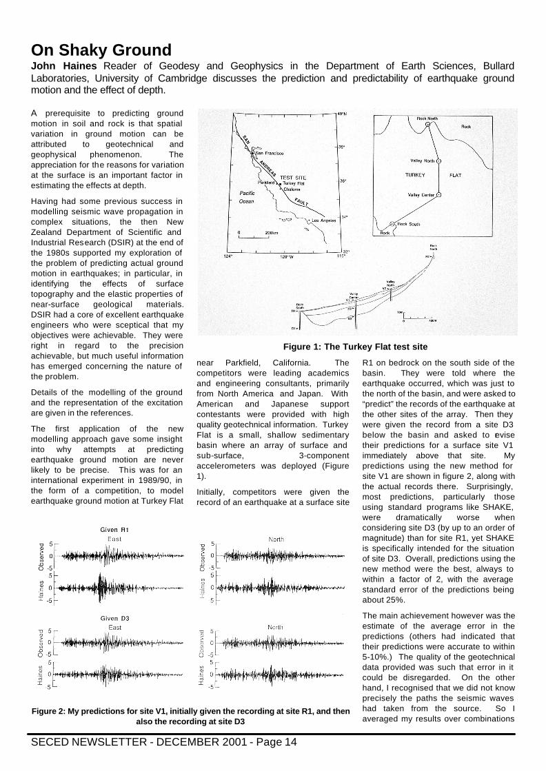
The first application of the new modelling approach gave some insight into why attempts at predicting earthquake ground motion are never likely to be precise. This was for an international experiment in 1989/90, in the form of a competition, to model earthquake ground motion at Turkey Flat
near Parkfield, California. The competitors were leading academics and engineering consultants, primarily from North America and Japan. With American and Japanese support contestants were provided with high quality geotechnical information. Turkey Flat is a small, shallow sedimentary basin where an array of surface and sub-surface, 3-component accelerometers was deployed (Figure 1).
Initially, competitors were given the record of an earthquake at a surface site
R1 on bedrock on the south side of the basin. They were told where the earthquake occurred, which was just to the north of the basin, and were asked to “predict” the records of the earthquake at the other sites of the array. Then they were given the record from a site D3 below the basin and asked to revise their predictions for a surface site V1 immediately above that site. My predictions using the new method for site V1 are shown in figure 2, along with the actual records there. Surprisingly, most predictions, particularly those using standard programs like SHAKE, were dramatically worse when considering site D3 (by up to an order of magnitude) than for site R1, yet SHAKE is specifically intended for the situation of site D3. Overall, predictions using the new method were the best, always to within a factor of 2, with the average standard error of the predictions being about 25%.
The main achievement however was the estimate of the average error in the predictions (others had indicated that their predictions were accurate to within 5-10%.) The quality of the geotechnical data provided was such that error in it could be disregarded. On the other hand, I recognised that we did not know precisely the paths the seismic waves had taken from the source. So I averaged my results over combinations
Figure 1: The Turkey Flat test site
Figure 2: My predictions for site V1, initially given the recording at site R1, and then also the recording at site D3
SECED NEWSLETTER - DECEMBER 2001 - Page 15
of angles of incidence at the array that were consistent with the records provided. Without the 3-component records from a site close to where the predictions were being made, the accuracy of the predictions would have been poorer.
For future earthquakes, nearby recordings of those earthquakes don't
already exist. What then was the point of the Turkey Flat experiment, other than fostering justifiable distrust of modelling predictions? Programs like SHAKE assume purely vertical propagation of the waves, which was clearly inappropriate to the situation at Turkey Flat. However, that alone does not explain the exceedingly poor accuracy of predictions using such programs. Programs that took into account the correct angles of incidence also were likely to perform moderately poorly if they did not allow properly for the sedimentary layers pinching out on each side of the basin and changing thickness slightly elsewhere.
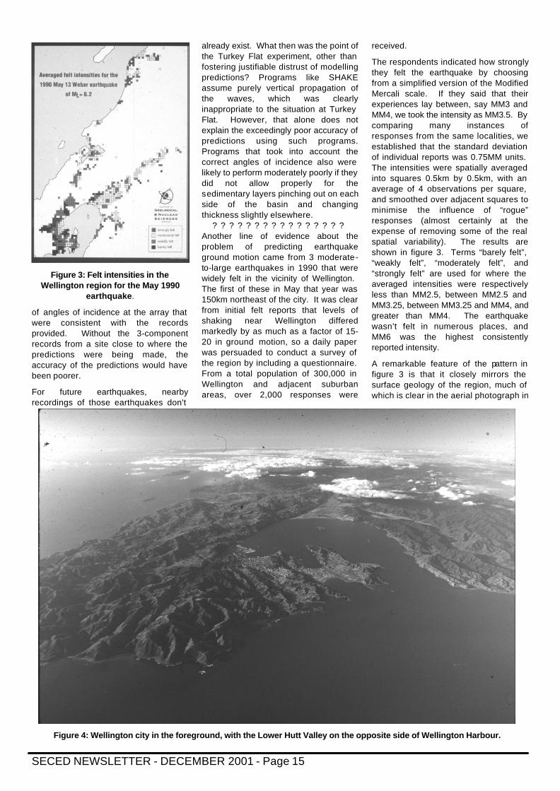
? ? ? ? ? ? ? ? ? ? ? ? ? ? ? ? Another line of evidence about the problem of predicting earthquake ground motion came from 3 moderate-to-large earthquakes in 1990 that were widely felt in the vicinity of Wellington. The first of these in May that year was 150km northeast of the city. It was clear from initial felt reports that levels of shaking near Wellington differed markedly by as much as a factor of 15-20 in ground motion, so a daily paper was persuaded to conduct a survey of the region by including a questionnaire. From a total population of 300,000 in Wellington and adjacent suburban areas, over 2,000 responses were
received.
The respondents indicated how strongly they felt the earthquake by choosing from a simplified version of the Modified Mercali scale. If they said that their experiences lay between, say MM3 and MM4, we took the intensity as MM3.5. By comparing many instances of responses from the same localities, we established that the standard deviation of individual reports was 0.75MM units. The intensities were spatially averaged into squares 0.5km by 0.5km, with an average of 4 observations per square, and smoothed over adjacent squares to minimise the influence of “rogue” responses (almost certainly at the expense of removing some of the real spatial variability). The results are shown in figure 3. Terms “barely felt”, “weakly felt”, “moderately felt”, and “strongly felt” are used for where the averaged intensities were respectively less than MM2.5, between MM2.5 and MM3.25, between MM3.25 and MM4, and greater than MM4. The earthquake wasn’t felt in numerous places, and MM6 was the highest consistently reported intensity.
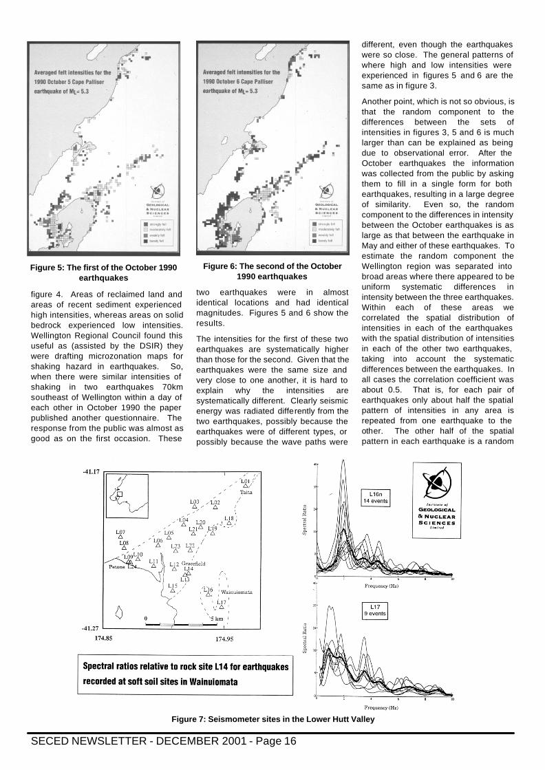
A remarkable feature of the pattern in figure 3 is that it closely mirrors the surface geology of the region, much of which is clear in the aerial photograph in
Figure 3: Felt intensities in the Wellington region for the May 1990
earthquake.
Figure 4: Wellington city in the foreground, with the Lower Hutt Valley on the opposite side of Wellington Harbour.
SECED NEWSLETTER - DECEMBER 2001 - Page 16
figure 4. Areas of reclaimed land and areas of recent sediment experienced high intensities, whereas areas on solid bedrock experienced low intensities. Wellington Regional Council found this useful as (assisted by the DSIR) they were drafting microzonation maps for shaking hazard in earthquakes. So, when there were similar intensities of shaking in two earthquakes 70km southeast of Wellington within a day of each other in October 1990 the paper published another questionnaire. The response from the public was almost as good as on the first occasion. These
two earthquakes were in almost identical locations and had identical magnitudes. Figures 5 and 6 show the results.
The intensities for the first of these two earthquakes are systematically higher than those for the second. Given that the earthquakes were the same size and very close to one another, it is hard to explain why the intensities are systematically different. Clearly seismic energy was radiated differently from the two earthquakes, possibly because the earthquakes were of different types, or possibly because the wave paths were
different, even though the earthquakes were so close. The general patterns of where high and low intensities were experienced in figures 5 and 6 are the same as in figure 3.
Another point, which is not so obvious, is that the random component to the differences between the sets of intensities in figures 3, 5 and 6 is much larger than can be explained as being due to observational error. After the October earthquakes the information was collected from the public by asking them to fill in a single form for both earthquakes, resulting in a large degree of similarity. Even so, the random component to the differences in intensity between the October earthquakes is as large as that between the earthquake in May and either of these earthquakes. To estimate the random component the Wellington region was separated into broad areas where there appeared to be uniform systematic differences in intensity between the three earthquakes. Within each of these areas we correlated the spatial distribution of intensities in each of the earthquakes with the spatial distribution of intensities in each of the other two earthquakes, taking into account the systematic differences between the earthquakes. In all cases the correlation coefficient was about 0.5. That is, for each pair of earthquakes only about half the spatial pattern of intensities in any area is repeated from one earthquake to the other. The other half of the spatial pattern in each earthquake is a random
Figure 5: The first of the October 1990 earthquakes
Figure 6: The second of the October 1990 earthquakes
Figure 7: Seismometer sites in the Lower Hutt Valley
SECED NEWSLETTER - DECEMBER 2001 - Page 17
distribution.
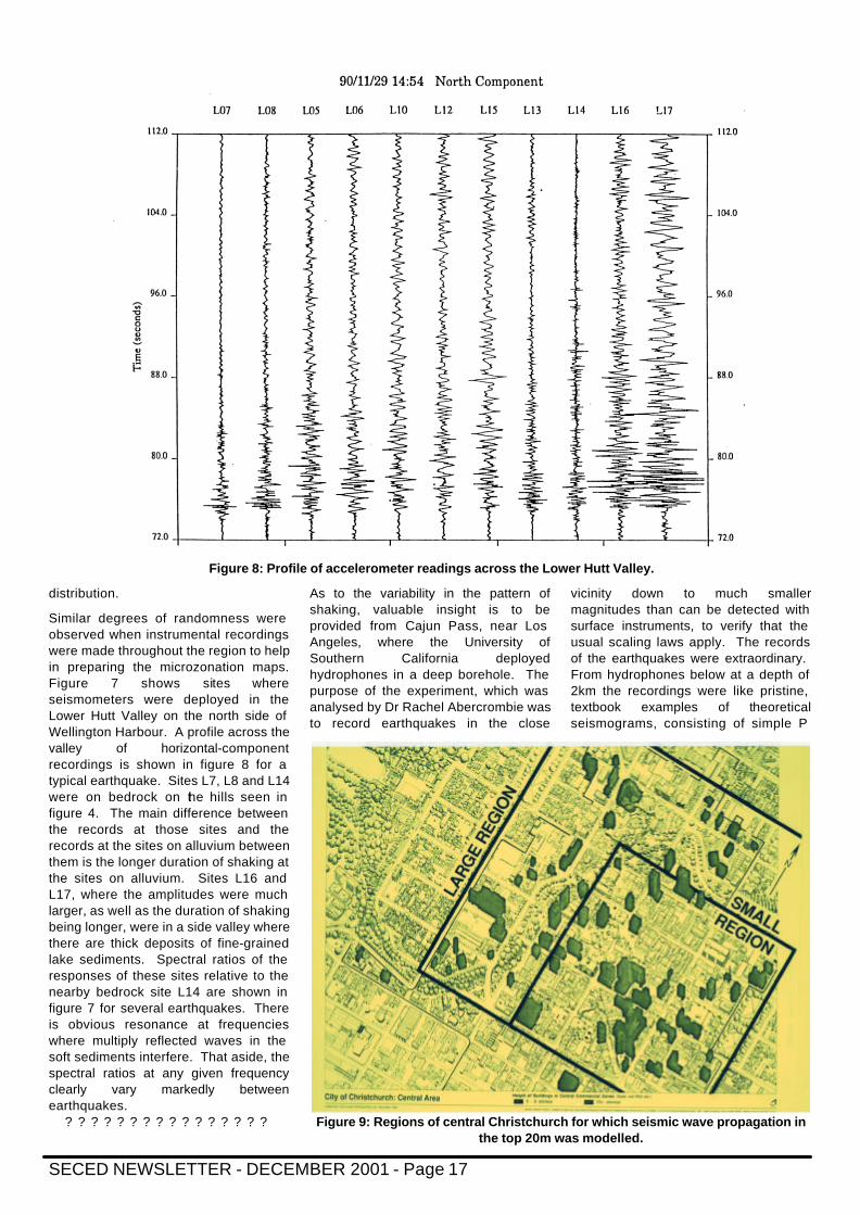
Similar degrees of randomness were observed when instrumental recordings were made throughout the region to help in preparing the microzonation maps. Figure 7 shows sites where seismometers were deployed in the Lower Hutt Valley on the north side of Wellington Harbour. A profile across the valley of horizontal-component recordings is shown in figure 8 for a typical earthquake. Sites L7, L8 and L14 were on bedrock on the hills seen in figure 4. The main difference between the records at those sites and the records at the sites on alluvium between them is the longer duration of shaking at the sites on alluvium. Sites L16 and L17, where the amplitudes were much larger, as well as the duration of shaking being longer, were in a side valley where there are thick deposits of fine-grained lake sediments. Spectral ratios of the responses of these sites relative to the nearby bedrock site L14 are shown in figure 7 for several earthquakes. There is obvious resonance at frequencies where multiply reflected waves in the soft sediments interfere. That aside, the spectral ratios at any given frequency clearly vary markedly between earthquakes.
? ? ? ? ? ? ? ? ? ? ? ? ? ? ? ?
As to the variability in the pattern of shaking, valuable insight is to be provided from Cajun Pass, near Los Angeles, where the University of Southern California deployed hydrophones in a deep borehole. The purpose of the experiment, which was analysed by Dr Rachel Abercrombie was to record earthquakes in the close
vicinity down to much smaller magnitudes than can be detected with surface instruments, to verify that the usual scaling laws apply. The records of the earthquakes were extraordinary. From hydrophones below at a depth of 2km the recordings were like pristine, textbook examples of theoretical seismograms, consisting of simple P
Figure 8: Profile of accelerometer readings across the Lower Hutt Valley.
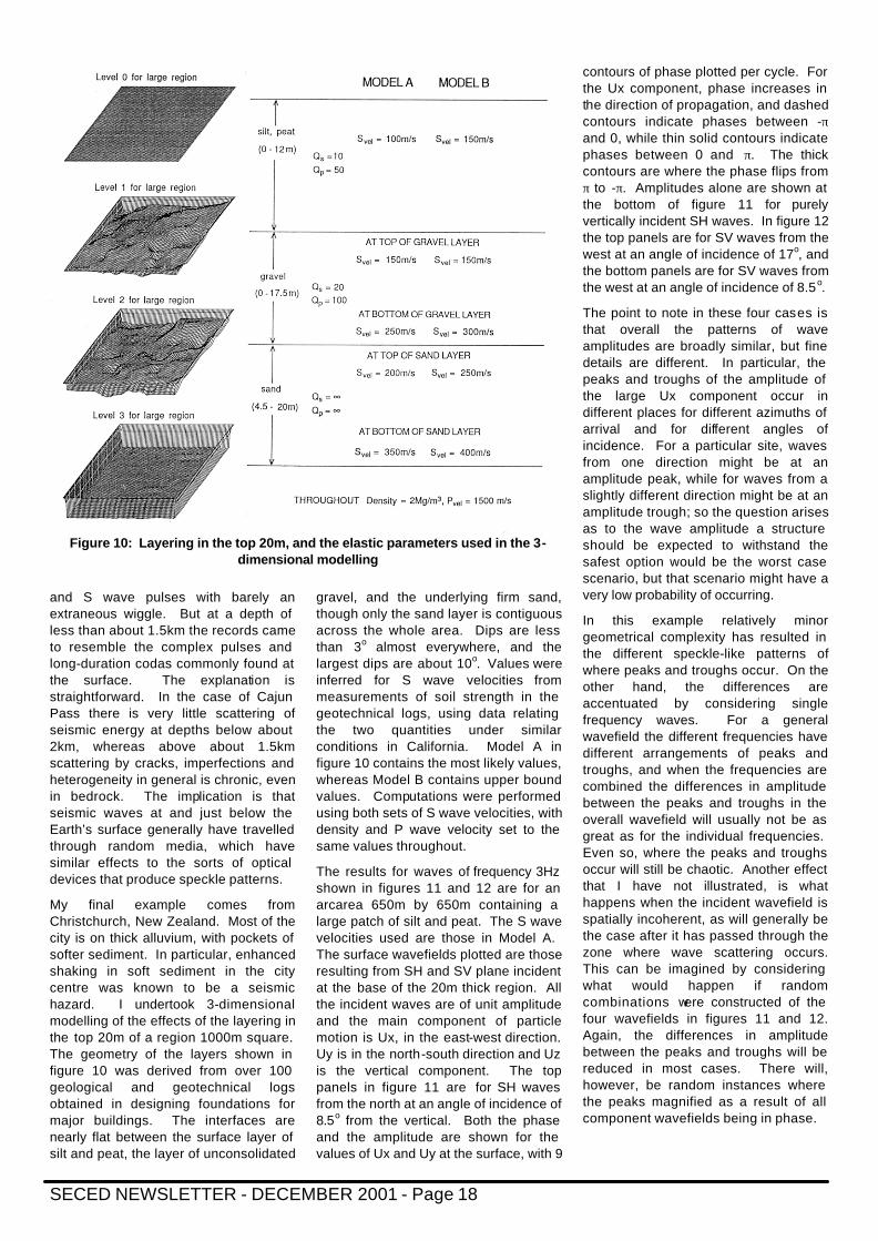
Figure 9: Regions of central Christchurch for which seismic wave propagation in
the top 20m was modelled.
SECED NEWSLETTER - DECEMBER 2001 - Page 18
and S wave pulses with barely an extraneous wiggle. But at a depth of less than about 1.5km the records came to resemble the complex pulses and long-duration codas commonly found at the surface. The explanation is straightforward. In the case of Cajun Pass there is very little scattering of seismic energy at depths below about 2km, whereas above about 1.5km scattering by cracks, imperfections and heterogeneity in general is chronic, even in bedrock. The implication is that seismic waves at and just below the Earth’s surface generally have travelled through random media, which have similar effects to the sorts of optical devices that produce speckle patterns.
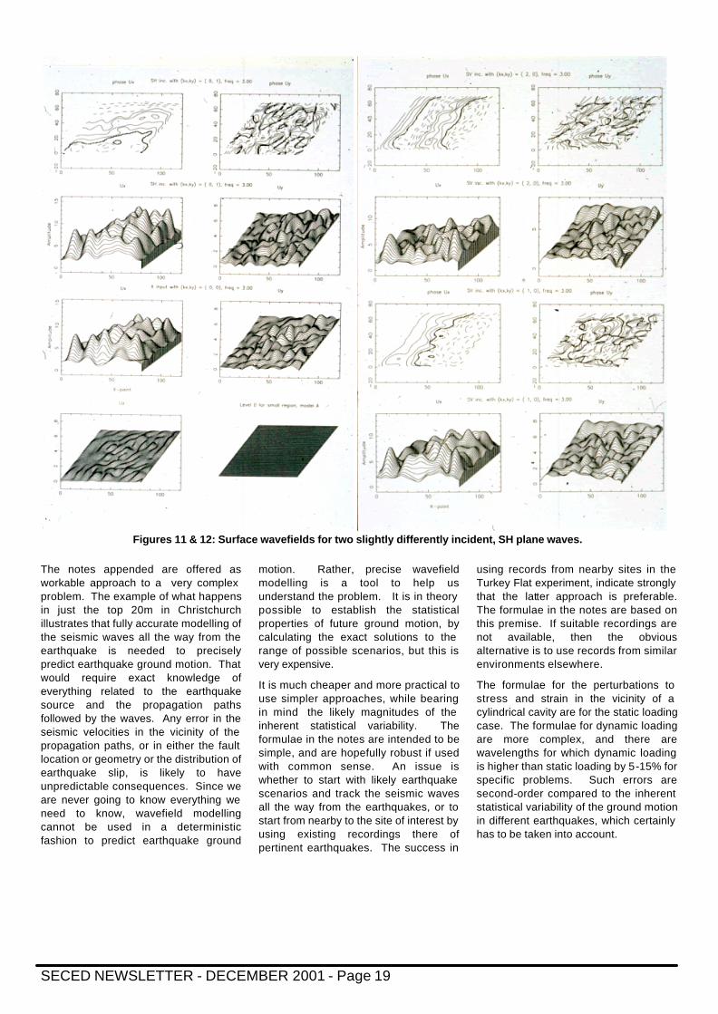
My final example comes from Christchurch, New Zealand. Most of the city is on thick alluvium, with pockets of softer sediment. In particular, enhanced shaking in soft sediment in the city centre was known to be a seismic hazard. I undertook 3-dimensional modelling of the effects of the layering in the top 20m of a region 1000m square. The geometry of the layers shown in figure 10 was derived from over 100 geological and geotechnical logs obtained in designing foundations for major buildings. The interfaces are nearly flat between the surface layer of silt and peat, the layer of unconsolidated
gravel, and the underlying firm sand, though only the sand layer is contiguous across the whole area. Dips are less than 3o almost everywhere, and the largest dips are about 10o. Values were inferred for S wave velocities from measurements of soil strength in the geotechnical logs, using data relating the two quantities under similar conditions in California. Model A in figure 10 contains the most likely values, whereas Model B contains upper bound values. Computations were performed using both sets of S wave velocities, with density and P wave velocity set to the same values throughout.
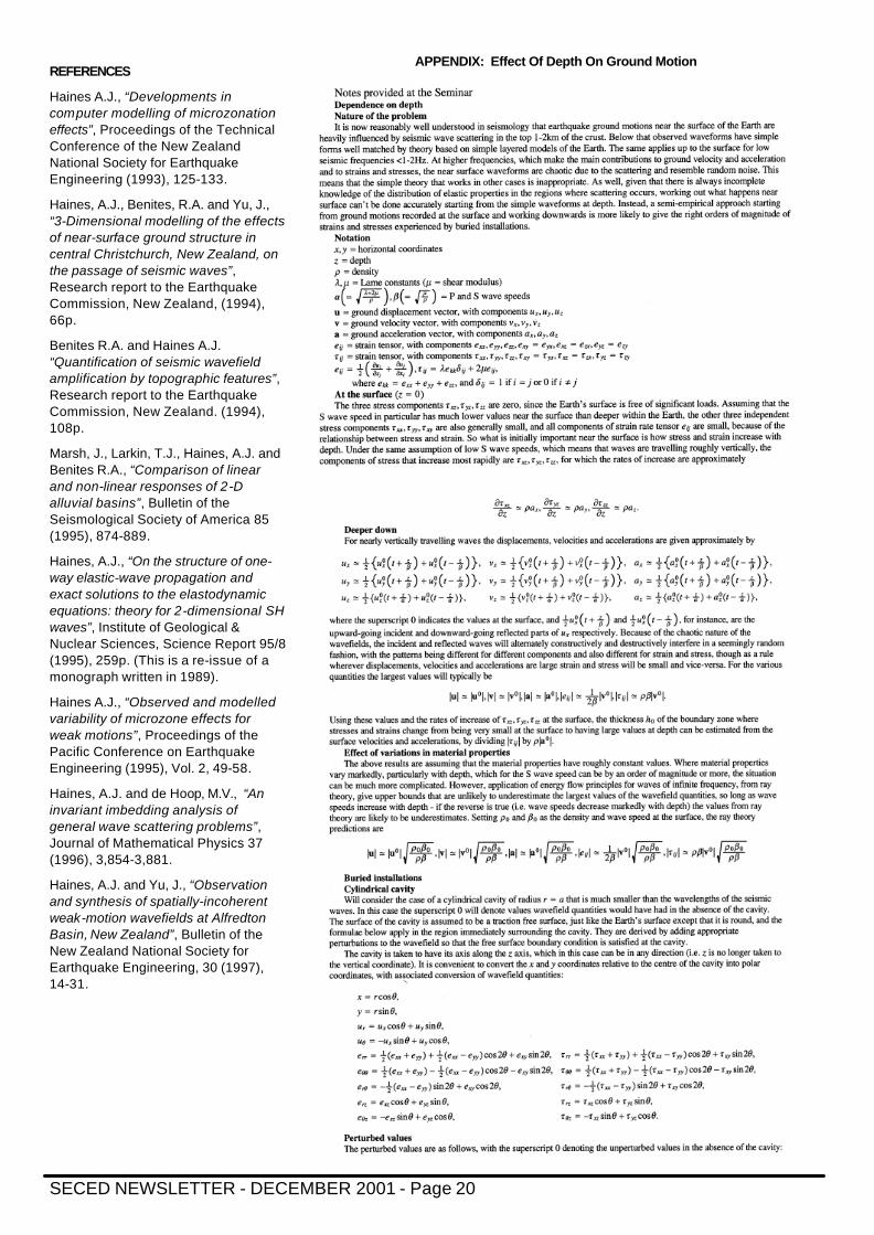
The results for waves of frequency 3Hz shown in figures 11 and 12 are for an arcarea 650m by 650m containing a large patch of silt and peat. The S wave velocities used are those in Model A. The surface wavefields plotted are those resulting from SH and SV plane incident at the base of the 20m thick region. All the incident waves are of unit amplitude and the main component of particle motion is Ux, in the east-west direction. Uy is in the north-south direction and Uz is the vertical component. The top panels in figure 11 are for SH waves from the north at an angle of incidence of 8.5o from the vertical. Both the phase and the amplitude are shown for the values of Ux and Uy at the surface, with 9
contours of phase plotted per cycle. For the Ux component, phase increases in the direction of propagation, and dashed contours indicate phases between -π and 0, while thin solid contours indicate phases between 0 and π. The thick contours are where the phase flips from π to -π. Amplitudes alone are shown at the bottom of figure 11 for purely vertically incident SH waves. In figure 12 the top panels are for SV waves from the west at an angle of incidence of 17o, and the bottom panels are for SV waves from the west at an angle of incidence of 8.5o.
The point to note in these four cases is that overall the patterns of wave amplitudes are broadly similar, but fine details are different. In particular, the peaks and troughs of the amplitude of the large Ux component occur in different places for different azimuths of arrival and for different angles of incidence. For a particular site, waves from one direction might be at an amplitude peak, while for waves from a slightly different direction might be at an amplitude trough; so the question arises as to the wave amplitude a structure should be expected to withstand the safest option would be the worst case scenario, but that scenario might have a very low probability of occurring.
In this example relatively minor geometrical complexity has resulted in the different speckle-like patterns of where peaks and troughs occur. On the other hand, the differences are accentuated by considering single frequency waves. For a general wavefield the different frequencies have different arrangements of peaks and troughs, and when the frequencies are combined the differences in amplitude between the peaks and troughs in the overall wavefield will usually not be as great as for the individual frequencies. Even so, where the peaks and troughs occur will still be chaotic. Another effect that I have not illustrated, is what happens when the incident wavefield is spatially incoherent, as will generally be the case after it has passed through the zone where wave scattering occurs. This can be imagined by considering what would happen if random combinations were constructed of the four wavefields in figures 11 and 12. Again, the differences in amplitude between the peaks and troughs will be reduced in most cases. There will, however, be random instances where the peaks magnified as a result of all component wavefields being in phase.
Figure 10: Layering in the top 20m, and the elastic parameters used in the 3-
dimensional modelling
SECED NEWSLETTER - DECEMBER 2001 - Page 19
The notes appended are offered as workable approach to a very complex problem. The example of what happens in just the top 20m in Christchurch illustrates that fully accurate modelling of the seismic waves all the way from the earthquake is needed to precisely predict earthquake ground motion. That would require exact knowledge of everything related to the earthquake source and the propagation paths followed by the waves. Any error in the seismic velocities in the vicinity of the propagation paths, or in either the fault location or geometry or the distribution of earthquake slip, is likely to have unpredictable consequences. Since we are never going to know everything we need to know, wavefield modelling cannot be used in a deterministic fashion to predict earthquake ground
motion. Rather, precise wavefield modelling is a tool to help us understand the problem. It is in theory possible to establish the statistical properties of future ground motion, by calculating the exact solutions to the range of possible scenarios, but this is very expensive.
It is much cheaper and more practical to use simpler approaches, while bearing in mind the likely magnitudes of the inherent statistical variability. The formulae in the notes are intended to be simple, and are hopefully robust if used with common sense. An issue is whether to start with likely earthquake scenarios and track the seismic waves all the way from the earthquakes, or to start from nearby to the site of interest by using existing recordings there of pertinent earthquakes. The success in
using records from nearby sites in the Turkey Flat experiment, indicate strongly that the latter approach is preferable. The formulae in the notes are based on this premise. If suitable recordings are not available, then the obvious alternative is to use records from similar environments elsewhere.
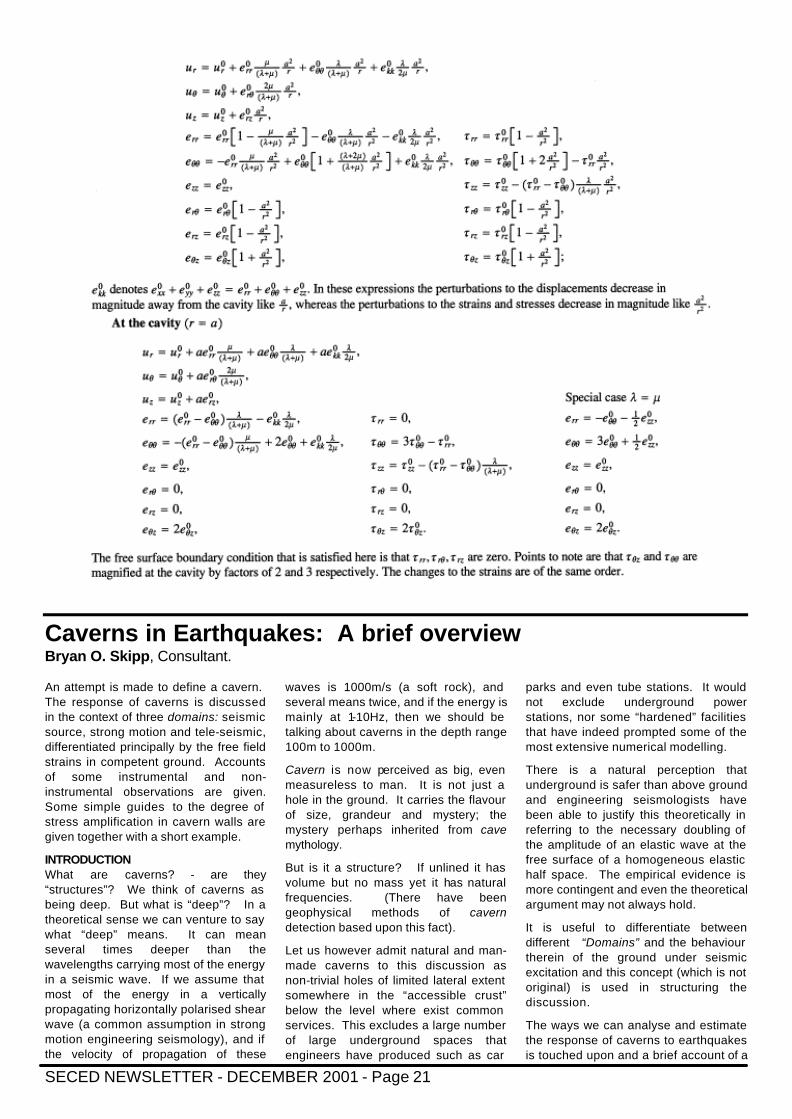
The formulae for the perturbations to stress and strain in the vicinity of a cylindrical cavity are for the static loading case. The formulae for dynamic loading are more complex, and there are wavelengths for which dynamic loading is higher than static loading by 5-15% for specific problems. Such errors are second-order compared to the inherent statistical variability of the ground motion in different earthquakes, which certainly has to be taken into account.
Figures 11 & 12: Surface wavefields for two slightly differently incident, SH plane waves.
SECED NEWSLETTER - DECEMBER 2001 - Page 20
REFERENCES
Haines A.J., “Developments in computer modelling of microzonation effects”, Proceedings of the Technical Conference of the New Zealand National Society for Earthquake Engineering (1993), 125-133.
Haines, A.J., Benites, R.A. and Yu, J., “3-Dimensional modelling of the effects of near-surface ground structure in central Christchurch, New Zealand, on the passage of seismic waves”, Research report to the Earthquake Commission, New Zealand, (1994), 66p.
Benites R.A. and Haines A.J. “Quantification of seismic wavefield amplification by topographic features”, Research report to the Earthquake Commission, New Zealand. (1994), 108p.
Marsh, J., Larkin, T.J., Haines, A.J. and Benites R.A., “Comparison of linear and non-linear responses of 2-D alluvial basins”, Bulletin of the Seismological Society of America 85 (1995), 874-889.
Haines, A.J., “On the structure of one-way elastic-wave propagation and exact solutions to the elastodynamic equations: theory for 2-dimensional SH waves”, Institute of Geological & Nuclear Sciences, Science Report 95/8 (1995), 259p. (This is a re-issue of a monograph written in 1989).
Haines A.J., “Observed and modelled variability of microzone effects for weak motions”, Proceedings of the Pacific Conference on Earthquake Engineering (1995), Vol. 2, 49-58.
Haines, A.J. and de Hoop, M.V., “An invariant imbedding analysis of general wave scattering problems”, Journal of Mathematical Physics 37 (1996), 3,854-3,881.
Haines, A.J. and Yu, J., “Observation and synthesis of spatially-incoherent weak-motion wavefields at Alfredton Basin, New Zealand”, Bulletin of the New Zealand National Society for Earthquake Engineering, 30 (1997), 14-31.
APPENDIX: Effect Of Depth On Ground Motion
SECED NEWSLETTER - DECEMBER 2001 - Page 21
Caverns in Earthquakes: A brief overview Bryan O. Skipp, Consultant. An attempt is made to define a cavern. The response of caverns is discussed in the context of three domains: seismic source, strong motion and tele-seismic, differentiated principally by the free field strains in competent ground. Accounts of some instrumental and non-instrumental observations are given. Some simple guides to the degree of stress amplification in cavern walls are given together with a short example.
INTRODUCTION What are caverns? - are they “structures”? We think of caverns as being deep. But what is “deep”? In a theoretical sense we can venture to say what “deep” means. It can mean several times deeper than the wavelengths carrying most of the energy in a seismic wave. If we assume that most of the energy in a vertically propagating horizontally polarised shear wave (a common assumption in strong motion engineering seismology), and if the velocity of propagation of these
waves is 1000m/s (a soft rock), and several means twice, and if the energy is mainly at 1-10Hz, then we should be talking about caverns in the depth range 100m to 1000m.
Cavern is now perceived as big, even measureless to man. It is not just a hole in the ground. It carries the flavour of size, grandeur and mystery; the mystery perhaps inherited from cave mythology.
But is it a structure? If unlined it has volume but no mass yet it has natural frequencies. (There have been geophysical methods of cavern detection based upon this fact).
Let us however admit natural and man-made caverns to this discussion as non-trivial holes of limited lateral extent somewhere in the “accessible crust” below the level where exist common services. This excludes a large number of large underground spaces that engineers have produced such as car
parks and even tube stations. It would not exclude underground power stations, nor some “hardened” facilities that have indeed prompted some of the most extensive numerical modelling.
There is a natural perception that underground is safer than above ground and engineering seismologists have been able to justify this theoretically in referring to the necessary doubling of the amplitude of an elastic wave at the free surface of a homogeneous elastic half space. The empirical evidence is more contingent and even the theoretical argument may not always hold.
It is useful to differentiate between different “Domains” and the behaviour therein of the ground under seismic excitation and this concept (which is not original) is used in structuring the discussion.
The ways we can analyse and estimate the response of caverns to earthquakes is touched upon and a brief account of a
SECED NEWSLETTER - DECEMBER 2001 - Page 22
“back of the envelope“ approach to a problem of the vulnerability of very large and deep caverns in a large solution salt mine in the giant Mirova diapir in Bulgaria is given.
The terminology in this paper is as defined in Skipp (1992).
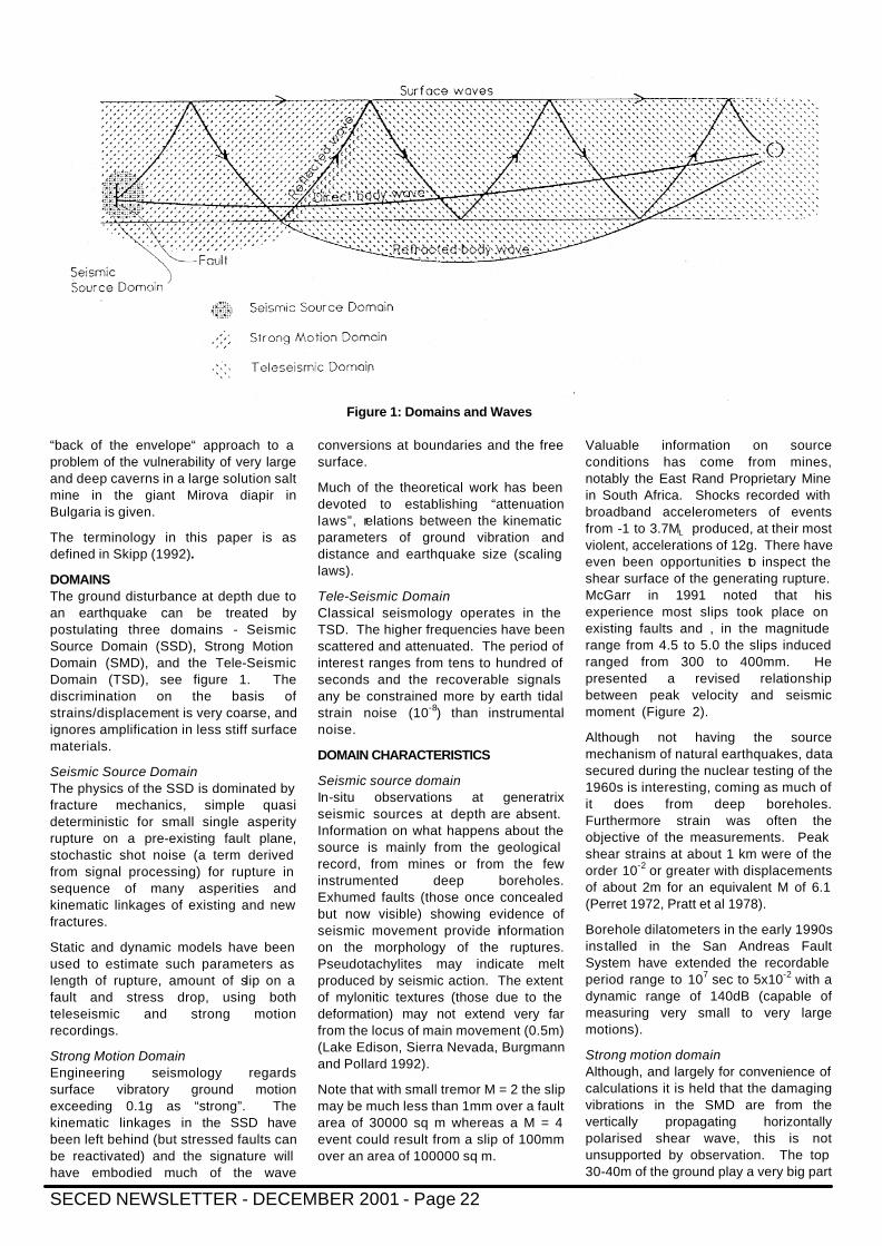
DOMAINS The ground disturbance at depth due to an earthquake can be treated by postulating three domains - Seismic Source Domain (SSD), Strong Motion Domain (SMD), and the Tele-Seismic Domain (TSD), see figure 1. The discrimination on the basis of strains/displacement is very coarse, and ignores amplification in less stiff surface materials.
Seismic Source Domain The physics of the SSD is dominated by fracture mechanics, simple quasi deterministic for small single asperity rupture on a pre-existing fault plane, stochastic shot noise (a term derived from signal processing) for rupture in sequence of many asperities and kinematic linkages of existing and new fractures.
Static and dynamic models have been used to estimate such parameters as length of rupture, amount of slip on a fault and stress drop, using both teleseismic and strong motion recordings.
Strong Motion Domain Engineering seismology regards surface vibratory ground motion exceeding 0.1g as “strong”. The kinematic linkages in the SSD have been left behind (but stressed faults can be reactivated) and the signature will have embodied much of the wave
conversions at boundaries and the free surface.
Much of the theoretical work has been devoted to establishing “attenuation laws”, relations between the kinematic parameters of ground vibration and distance and earthquake size (scaling laws).
Tele-Seismic Domain Classical seismology operates in the TSD. The higher frequencies have been scattered and attenuated. The period of interest ranges from tens to hundred of seconds and the recoverable signals any be constrained more by earth tidal strain noise (10-8) than instrumental noise.
DOMAIN CHARACTERISTICS
Seismic source domain In-situ observations at generatrix seismic sources at depth are absent. Information on what happens about the source is mainly from the geological record, from mines or from the few instrumented deep boreholes. Exhumed faults (those once concealed but now visible) showing evidence of seismic movement provide information on the morphology of the ruptures. Pseudotachylites may indicate melt produced by seismic action. The extent of mylonitic textures (those due to the deformation) may not extend very far from the locus of main movement (0.5m) (Lake Edison, Sierra Nevada, Burgmann and Pollard 1992).
Note that with small tremor M = 2 the slip may be much less than 1mm over a fault area of 30000 sq m whereas a M = 4 event could result from a slip of 100mm over an area of 100000 sq m.
Valuable information on source conditions has come from mines, notably the East Rand Proprietary Mine in South Africa. Shocks recorded with broadband accelerometers of events from -1 to 3.7ML produced, at their most violent, accelerations of 12g. There have even been opportunities to inspect the shear surface of the generating rupture. McGarr in 1991 noted that his experience most slips took place on existing faults and , in the magnitude range from 4.5 to 5.0 the slips induced ranged from 300 to 400mm. He presented a revised relationship between peak velocity and seismic moment (Figure 2).
Although not having the source mechanism of natural earthquakes, data secured during the nuclear testing of the 1960s is interesting, coming as much of it does from deep boreholes. Furthermore strain was often the objective of the measurements. Peak shear strains at about 1 km were of the order 10-2 or greater with displacements of about 2m for an equivalent M of 6.1 (Perret 1972, Pratt et al 1978).
Borehole dilatometers in the early 1990s installed in the San Andreas Fault System have extended the recordable period range to 107 sec to 5x10⁻² with a dynamic range of 140dB (capable of measuring very small to very large motions).
Strong motion domain Although, and largely for convenience of calculations it is held that the damaging vibrations in the SMD are from the vertically propagating horizontally polarised shear wave, this is not unsupported by observation. The top 30-40m of the ground play a very big part
Figure 1: Domains and Waves
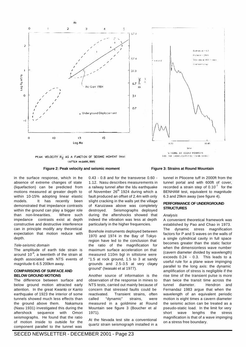
SECED NEWSLETTER - DECEMBER 2001 - Page 23
in the surface response, which in the absence of extreme changes of state (liquefaction) can be predicted from motions measured at greater depth to within 10-15% adopting linear elastic models. It has recently been demonstrated that impedance contrasts within the ground can play a bigger role than non-linearities. Where such impedance contrasts exist at depth constructive and destructive interference can in principle modify any theoretical expectation that motion reduce with depth.
Tele-seismic domain The amplitude of earth tide strain is around 10-8, a twentieth of the strain at depth associated with NTS events of magnitude 6-6.5 200km away.
COMPARISONS OF SURFACE AND BELOW GROUND MOTIONS The difference between surface and below ground motion attracted early attention. In the great Kwanto or Kanto earthquake of 1923 the interior of some tunnels showed much less effects than the ground above them. Nakamura (Nasu 1931) investigated this during the aftershock sequence with Omori seismographs. He found that the ratio of motion inside to outside for the component parallel to the tunnel was
0.43 - 0.8 and for the transverse 0.60 - 1.12. Nasu describes measurements in a railway tunnel after the Idu earthquake of November 26th 1924 during which a fault produced an offset of 2.4m with only slight cracking in the walls yet the village of Karuizawa above was completely destroyed. Seismographs deployed during the aftershocks showed that indeed the vibration was less at depth particularly in the higher frequencies.
Borehole instruments deployed between 1970 and 1974 in the Bay of Tokyo region have led to the conclusion that the ratio of the magnification for maximum surface acceleration on that measured 110m bgl in siltstone were “1.5 at rock ground, 1.5 to 3 at sandy grounds and 2.5-3.5 at very clayey ground” (Iwasaki et al 1977).
Another source of information is the observation of the response in mines to NTS tests, carried out mainly because of concern that stressed faults could be reactivated. Transient strains, often called “dynamic” strains, were measured in a goldmine at Round Mountain see figure 3 (Boucher et al 1971).
At the Nevada test site a conventional quartz strain seismograph installed in a
tunnel in Pliocene tuff in 2000ft from the tunnel portal and with 600ft of cover, recorded a strain step of 0.10-7 for the BENHAM test, equivalent to magnitude 6.3 and 29km away (see figure 4).
PERFORMANCE OF UNDERGROUND STRUCTURES
Analysis A convenient theoretical framework was established by Pao and Chao in 1973. The dynamic stress magnification factors for P and S waves on the walls of a single cylindrical cavity in full space becomes greater than the static factor when the dimensionless wave number (cavern diameter divided by wavelength) exceeds 0.24 - 0.3. This leads to a useful rule for a plane wave impinging parallel to the long axis: the dynamic amplification of stress is negligible if the rise time of the transient pulse is more than twice the transit time across the tunnel diameter. Hendron and Fernandaz 1983 argue that when the wavelength of an equivalent periodic motion is eight times a cavern diameter the seismic action can be treated as a pseudo-static load. In the limit for very short wave lengths the stress magnification is that of a wave impinging on a stress free boundary.
Figure 2: Peak velocity and seismic moment Figure 3: Strains at Round Mountain
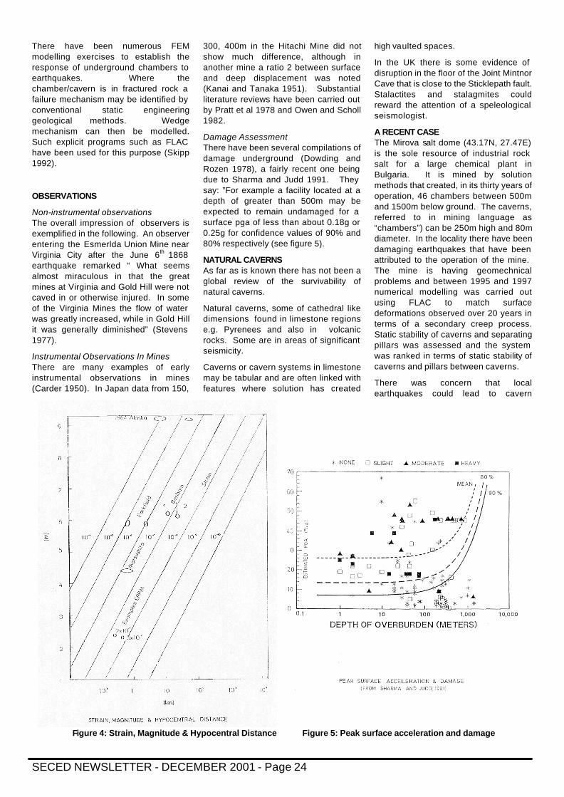
SECED NEWSLETTER - DECEMBER 2001 - Page 24
There have been numerous FEM modelling exercises to establish the response of underground chambers to earthquakes. Where the chamber/cavern is in fractured rock a failure mechanism may be identified by conventional static engineering geological methods. Wedge mechanism can then be modelled. Such explicit programs such as FLAC have been used for this purpose (Skipp 1992).
OBSERVATIONS
Non-instrumental observations The overall impression of observers is exemplified in the following. An observer entering the Esmerlda Union Mine near Virginia City after the June 6th 1868 earthquake remarked “ What seems almost miraculous in that the great mines at Virginia and Gold Hill were not caved in or otherwise injured. In some of the Virginia Mines the flow of water was greatly increased, while in Gold Hill it was generally diminished” (Stevens 1977).
Instrumental Observations In Mines There are many examples of early instrumental observations in mines (Carder 1950). In Japan data from 150,
300, 400m in the Hitachi Mine did not show much difference, although in another mine a ratio 2 between surface and deep displacement was noted (Kanai and Tanaka 1951). Substantial literature reviews have been carried out by Pratt et al 1978 and Owen and Scholl 1982.
Damage Assessment There have been several compilations of damage underground (Dowding and Rozen 1978), a fairly recent one being due to Sharma and Judd 1991. They say: ”For example a facility located at a depth of greater than 500m may be expected to remain undamaged for a surface pga of less than about 0.18g or 0.25g for confidence values of 90% and 80% respectively (see figure 5).
NATURAL CAVERNS As far as is known there has not been a global review of the survivability of natural caverns.
Natural caverns, some of cathedral like dimensions found in limestone regions e.g. Pyrenees and also in volcanic rocks. Some are in areas of significant seismicity.
Caverns or cavern systems in limestone may be tabular and are often linked with features where solution has created
high vaulted spaces.
In the UK there is some evidence of disruption in the floor of the Joint Mintnor Cave that is close to the Sticklepath fault. Stalactites and stalagmites could reward the attention of a speleological seismologist.
A RECENT CASE The Mirova salt dome (43.17N, 27.47E) is the sole resource of industrial rock salt for a large chemical plant in Bulgaria. It is mined by solution methods that created, in its thirty years of operation, 46 chambers between 500m and 1500m below ground. The caverns, referred to in mining language as “chambers”) can be 250m high and 80m diameter. In the locality there have been damaging earthquakes that have been attributed to the operation of the mine. The mine is having geomechnical problems and between 1995 and 1997 numerical modelling was carried out using FLAC to match surface deformations observed over 20 years in terms of a secondary creep process. Static stability of caverns and separating pillars was assessed and the system was ranked in terms of static stability of caverns and pillars between caverns.
There was concern that local earthquakes could lead to cavern
Figure 4: Strain, Magnitude & Hypocentral Distance Figure 5: Peak surface acceleration and damage
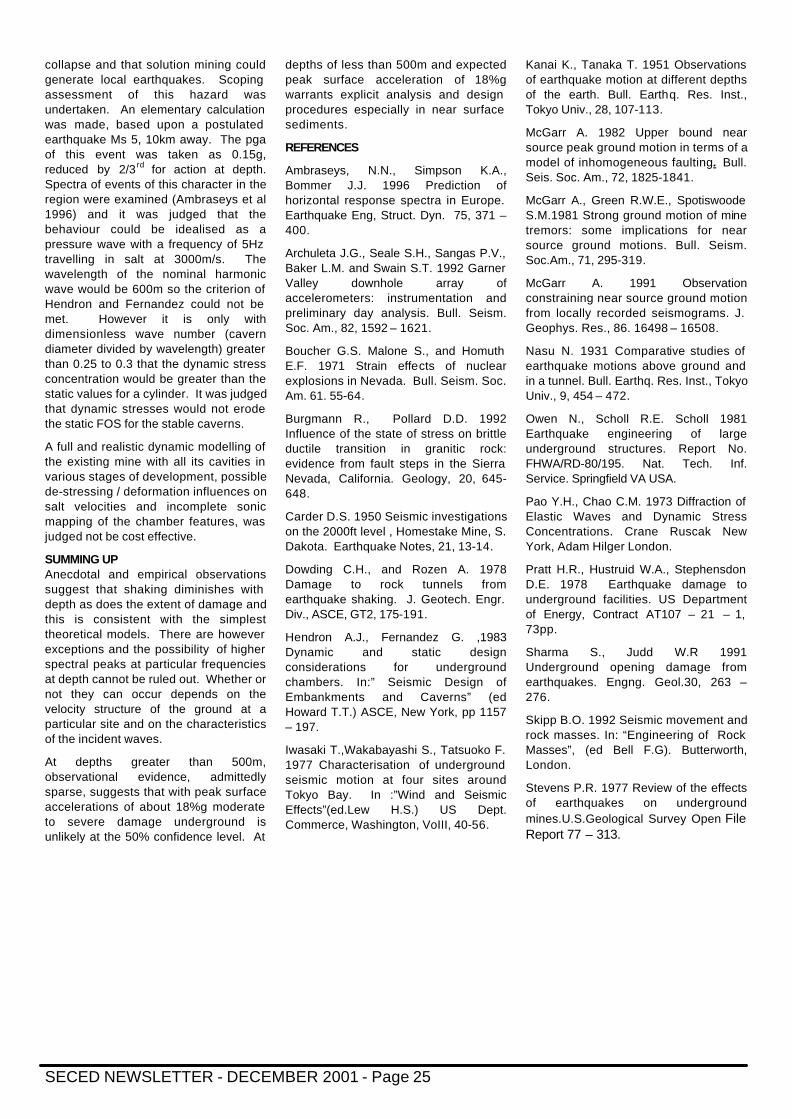
SECED NEWSLETTER - DECEMBER 2001 - Page 25
collapse and that solution mining could generate local earthquakes. Scoping assessment of this hazard was undertaken. An elementary calculation was made, based upon a postulated earthquake Ms 5, 10km away. The pga of this event was taken as 0.15g, reduced by 2/3 rd for action at depth. Spectra of events of this character in the region were examined (Ambraseys et al 1996) and it was judged that the behaviour could be idealised as a pressure wave with a frequency of 5Hz travelling in salt at 3000m/s. The wavelength of the nominal harmonic wave would be 600m so the criterion of Hendron and Fernandez could not be met. However it is only with dimensionless wave number (cavern diameter divided by wavelength) greater than 0.25 to 0.3 that the dynamic stress concentration would be greater than the static values for a cylinder. It was judged that dynamic stresses would not erode the static FOS for the stable caverns.
A full and realistic dynamic modelling of the existing mine with all its cavities in various stages of development, possible de-stressing / deformation influences on salt velocities and incomplete sonic mapping of the chamber features, was judged not be cost effective.
SUMMING UP Anecdotal and empirical observations suggest that shaking diminishes with depth as does the extent of damage and this is consistent with the simplest theoretical models. There are however exceptions and the possibility of higher spectral peaks at particular frequencies at depth cannot be ruled out. Whether or not they can occur depends on the velocity structure of the ground at a particular site and on the characteristics of the incident waves.
At depths greater than 500m, observational evidence, admittedly sparse, suggests that with peak surface accelerations of about 18%g moderate to severe damage underground is unlikely at the 50% confidence level. At
depths of less than 500m and expected peak surface acceleration of 18%g warrants explicit analysis and design procedures especially in near surface sediments.
REFERENCES
Ambraseys, N.N., Simpson K.A., Bommer J.J. 1996 Prediction of horizontal response spectra in Europe. Earthquake Eng, Struct. Dyn. 75, 371 – 400.
Archuleta J.G., Seale S.H., Sangas P.V., Baker L.M. and Swain S.T. 1992 Garner Valley downhole array of accelerometers: instrumentation and preliminary day analysis. Bull. Seism. Soc. Am., 82, 1592 – 1621.
Boucher G.S. Malone S., and Homuth E.F. 1971 Strain effects of nuclear explosions in Nevada. Bull. Seism. Soc. Am. 61. 55-64.
Burgmann R., Pollard D.D. 1992 Influence of the state of stress on brittle ductile transition in granitic rock: evidence from fault steps in the Sierra Nevada, California. Geology, 20, 645-648.
Carder D.S. 1950 Seismic investigations on the 2000ft level , Homestake Mine, S. Dakota. Earthquake Notes, 21, 13-14.
Dowding C.H., and Rozen A. 1978 Damage to rock tunnels from earthquake shaking. J. Geotech. Engr. Div., ASCE, GT2, 175-191.
Hendron A.J., Fernandez G. ,1983 Dynamic and static design considerations for underground chambers. In:” Seismic Design of Embankments and Caverns” (ed Howard T.T.) ASCE, New York, pp 1157 – 197.
Iwasaki T.,Wakabayashi S., Tatsuoko F. 1977 Characterisation of underground seismic motion at four sites around Tokyo Bay. In :”Wind and Seismic Effects”(ed.Lew H.S.) US Dept. Commerce, Washington, VoIII, 40-56.
Kanai K., Tanaka T. 1951 Observations of earthquake motion at different depths of the earth. Bull. Earthq. Res. Inst., Tokyo Univ., 28, 107-113.
McGarr A. 1982 Upper bound near source peak ground motion in terms of a model of inhomogeneous faulting. Bull. Seis. Soc. Am., 72, 1825-1841.
McGarr A., Green R.W.E., Spotiswoode S.M.1981 Strong ground motion of mine tremors: some implications for near source ground motions. Bull. Seism. Soc.Am., 71, 295-319.
McGarr A. 1991 Observation constraining near source ground motion from locally recorded seismograms. J. Geophys. Res., 86. 16498 – 16508.
Nasu N. 1931 Comparative studies of earthquake motions above ground and in a tunnel. Bull. Earthq. Res. Inst., Tokyo Univ., 9, 454 – 472.
Owen N., Scholl R.E. Scholl 1981 Earthquake engineering of large underground structures. Report No. FHWA/RD-80/195. Nat. Tech. Inf. Service. Springfield VA USA.
Pao Y.H., Chao C.M. 1973 Diffraction of Elastic Waves and Dynamic Stress Concentrations. Crane Ruscak New York, Adam Hilger London.
Pratt H.R., Hustruid W.A., Stephensdon D.E. 1978 Earthquake damage to underground facilities. US Department of Energy, Contract AT107 – 21 – 1, 73pp.
Sharma S., Judd W.R 1991 Underground opening damage from earthquakes. Engng. Geol.30, 263 – 276.
Skipp B.O. 1992 Seismic movement and rock masses. In: “Engineering of Rock Masses”, (ed Bell F.G). Butterworth, London.
Stevens P.R. 1977 Review of the effects of earthquakes on underground mines.U.S.Geological Survey Open File Report 77 – 313.
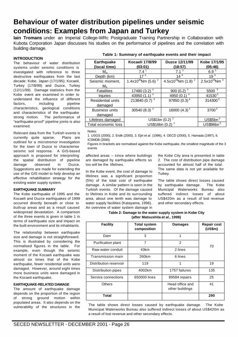
SECED NEWSLETTER - DECEMBER 2001 - Page 26
Behaviour of water distribution pipelines under seismic conditions: Examples from Japan and Turkey Iain Tromans under an Imperial College-WRc Postgraduate Training Partnership in Collaboration with Kubota Corporation Japan discusses his studies on the performance of pipelines and the correlation with building damage. INTRODUCTION The behaviour of water distribution systems under seismic conditions is investigated with reference to three destructive earthquakes from the last decade: Kobe, Japan (17/1/95); Kocaeli, Turkey (17/8/99) and Duzce, Turkey (12/11/99). Damage statistics from the Kobe event are examined in order to understand the influence of different factors, including pipeline characteristics, geological conditions and characteristics of the earthquake strong motion. The performance of "earthquake-proof" pipeline joints is also examined.
Relevant data from the Turkish events is currently quite sparse. Plans are outlined for a microtremor investigation for the town of Duzce to characterise seismic soil response. A GIS-based approach is proposed for interpreting the spatial distribution of pipeline damage observed in Duzce. Suggestions are made for extending the use of the GIS model to help develop an effective rehabilitation strategy for the existing water supply system.
EARTHQUAKE SUMMARY The Kobe earthquake of 1995 and the Kocaeli and Duzce earthquakes of 1999 occurred directly beneath or close to built-up areas and as a result caused widespread devastation. A comparison of the three events is given in table 1 in terms of earthquake size and impact on the built environment and its inhabitants.
The relationship between earthquake size and damage is not straightforward. This is illustrated by considering the normalised figures in the table. For example, even though the seismic moment of the Kocaeli earthquake was almost six times that of the Kobe earthquake, fewer residential units were damaged. However, around eight times more business units were damaged in the Kocaeli earthquake.
EARTHQUAKE-RELATED DAMAGE The amount of earthquake damage depends on the proportion of the region of strong ground motion within populated areas. It also depends on the vulnerability of the structures in the
affected areas – since where buildings are damaged by earthquake effects so too will be the lifelines.
In the Kobe event, the cost of damage to lifelines was a significant proportion (5%) of the total cost of earthquake damage. A similar pattern is seen in the Turkish events. Of the damage caused to lifelines in Kobe and its surrounding area, about one tenth was damage to water supply facilities (Katayama, 1996). An overview of water system damage in
the Kobe City area is presented in table 2. The cost of distribution pipe damage accounted for almost half of the total. The same data is not yet available for Turkey.
The table shows direct losses caused by earthquake damage. The Kobe Municipal Waterworks Bureau also suffered indirect losses of about US$420m as a result of lost revenue and other secondary effects.
Table 1: Summary of earthquake events and their impact
Earthquake (local time)
Kocaeli 17/8/99 (03:01)
Duzce 12/11/99 (18:57)
Kobe 17/1/95 (05:46)
Mw 7.4 1 7.1 2 6.9 3
Depth (km) 17 6 14 6 19 6
Seismic moment, M0
1.4x10²⁰Nm (5.6) 2 4.5x10¹⁹Nm (1.8) 2 2.5x10¹⁹Nm 3
Fatalities 17480 (3.2) 4 900 (0.2) 4 5500 5
Injuries 43950 (1.1) 4 4950 (0.1) 4 41530 5
Residential units damaged
213840 (0.7) 4 97850 (0.3) 4 314300 5
Business units damaged
30540 (8.3) 4 16000 (4.3) 4 3700 5
Lifelines damaged US$5bn 5
Total economic loss US$1bn (0.2) 2
US$16bn (0.2) 2 US$96bn 5
Notes: 1. USGS (2000), 2. Erdik (2000), 3. Ejiri et al. (1996), 4. OECD (2000), 5. Hamada (1997), 6. ICSMDB (2000). Figures in brackets are normalised against the Kobe earthquake, the smallest magnitude of the 3 events
Table 2: Damage to the water supply system in Kobe City (after Matsushita et al., 1998)
Facility Total system composition
Damages Repair cost (US$m)
Dam 3 1
Purification plant 7 2
Raw water conduit 43km 2 lines
Transmission main 260km 6 lines
70
Distribution reservoir 119 1 19
Distribution pipes 4002km 1757 failures 135
Service connections 650000 lines 89584 repairs 25
Others Head office and other buildings
41
Total 290
The table shows direct losses caused by earthquake damage. The Kobe Municipal Waterworks Bureau also suffered indirect losses of about US$420m as a result of lost revenue and other secondary effects.
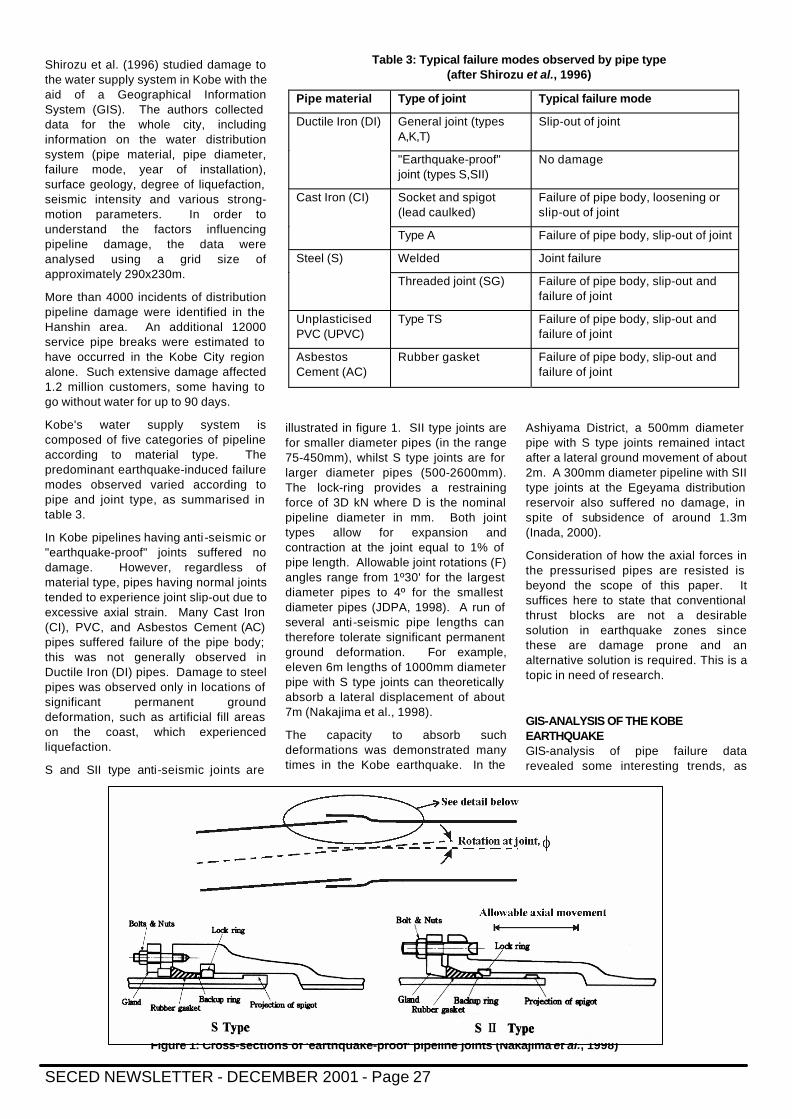
SECED NEWSLETTER - DECEMBER 2001 - Page 27
Shirozu et al. (1996) studied damage to the water supply system in Kobe with the aid of a Geographical Information System (GIS). The authors collected data for the whole city, including information on the water distribution system (pipe material, pipe diameter, failure mode, year of installation), surface geology, degree of liquefaction, seismic intensity and various strong-motion parameters. In order to understand the factors influencing pipeline damage, the data were analysed using a grid size of approximately 290x230m.
More than 4000 incidents of distribution pipeline damage were identified in the Hanshin area. An additional 12000 service pipe breaks were estimated to have occurred in the Kobe City region alone. Such extensive damage affected 1.2 million customers, some having to go without water for up to 90 days.
Kobe's water supply system is composed of five categories of pipeline according to material type. The predominant earthquake-induced failure modes observed varied according to pipe and joint type, as summarised in table 3.
In Kobe pipelines having anti -seismic or "earthquake-proof" joints suffered no damage. However, regardless of material type, pipes having normal joints tended to experience joint slip-out due to excessive axial strain. Many Cast Iron (CI), PVC, and Asbestos Cement (AC) pipes suffered failure of the pipe body; this was not generally observed in Ductile Iron (DI) pipes. Damage to steel pipes was observed only in locations of significant permanent ground deformation, such as artificial fill areas on the coast, which experienced liquefaction.
S and SII type anti-seismic joints are
illustrated in figure 1. SII type joints are for smaller diameter pipes (in the range 75-450mm), whilst S type joints are for larger diameter pipes (500-2600mm). The lock-ring provides a restraining force of 3D kN where D is the nominal pipeline diameter in mm. Both joint types allow for expansion and contraction at the joint equal to 1% of pipe length. Allowable joint rotations (F) angles range from 1º30' for the largest diameter pipes to 4º for the smallest diameter pipes (JDPA, 1998). A run of several anti-seismic pipe lengths can therefore tolerate significant permanent ground deformation. For example, eleven 6m lengths of 1000mm diameter pipe with S type joints can theoretically absorb a lateral displacement of about 7m (Nakajima et al., 1998).
The capacity to absorb such deformations was demonstrated many times in the Kobe earthquake. In the
Ashiyama District, a 500mm diameter pipe with S type joints remained intact after a lateral ground movement of about 2m. A 300mm diameter pipeline with SII type joints at the Egeyama distribution reservoir also suffered no damage, in spite of subsidence of around 1.3m (Inada, 2000).
Consideration of how the axial forces in the pressurised pipes are resisted is beyond the scope of this paper. It suffices here to state that conventional thrust blocks are not a desirable solution in earthquake zones since these are damage prone and an alternative solution is required. This is a topic in need of research.
GIS-ANALYSIS OF THE KOBE EARTHQUAKE GIS-analysis of pipe failure data revealed some interesting trends, as
Table 3: Typical failure modes observed by pipe type (after Shirozu et al., 1996)
Pipe material Type of joint Typical failure mode
General joint (types A,K,T)
Slip-out of joint Ductile Iron (DI)
"Earthquake-proof" joint (types S,SII)
No damage
Socket and spigot (lead caulked)
Failure of pipe body, loosening or slip-out of joint
Cast Iron (CI)
Type A Failure of pipe body, slip-out of joint
Welded Joint failure Steel (S)
Threaded joint (SG) Failure of pipe body, slip-out and failure of joint
Unplasticised PVC (UPVC)
Type TS Failure of pipe body, slip-out and failure of joint
Asbestos Cement (AC)
Rubber gasket Failure of pipe body, slip-out and failure of joint
Figure 1: Cross-sections of 'earthquake-proof' pipeline joints (Nakajima et al., 1998)
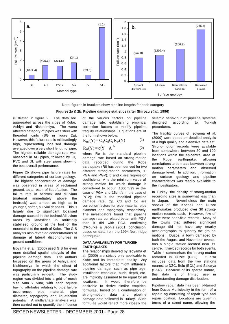
SECED NEWSLETTER - DECEMBER 2001 - Page 28
illustrated in figure 2. The data are aggregated across the cities of Kobe, Ashiya and Nishinomiya. The worst affected category of pipes was steel with threaded joints (SG in figure 2a). However, this failure rate is misleadingly high, representing localised damage averaged over a very short length of pipe. The highest reliable damage rate was observed in AC pipes, followed by CI, PVC and DI, with steel pipes showing the best overall performance.
Figure 2b shows pipe failure rates for different categories of surface geology. The highest concentration of damage was observed in areas of reclaimed ground, as a result of liquefaction. The failure rate in bedrock and diluvium (material immediately above the bedrock) was almost as high as in younger, softer, alluvial deposits. This is largely due to significant localised damage caused in the bedrock/diluvium areas by landslides in artificially stabilised ground at the foot of the mountains to the north of Kobe. The GIS analysis also revealed concentrations of damage at lateral discontinuities in ground conditions.
Isoyama et al. (2000) used GIS for even more detailed spatial analysis of the pipeline damage data. The authors focussed on the areas of Ashiya and Nishinomiya, in which the effect of topography on the pipeline damage rate was particularly evident. The study region was divided into a grid of mesh size 50m x 50m, with each square having attributes relating to pipe failure occurrence, pipe material, pipe diameter, topography and liquefaction potential. A multivariate analysis was then carried out to quantify the influence
of the various factors on pipeline damage rate, establishing empirical correction factors to modify pipeline fragility relationships. Equations are of the form shown below:
(Y)RCCC(Y)R 0gdpm = (1)
( )b0 AYc(Y)R −= (2)
where Ro is the standard pipeline damage rate based on strong-motion data recorded during the Kobe earthquake (R0 has been derived for two different strong-motion parameters, Y: PGA and PGV); b and c are regression coefficients; A is the minimum value of strong motion for which damage is considered to occur (100cm/s2 in the case of PGA and 15cm/s in the case of PGV); Rm is the modified pipeline damage rate; Cp, Cd and Cg are correction factors for pipe material, pipe diameter and topography respectively. The investigators found that pipeline damage rate correlated better with PGV than it did with PGA, confirming O'Rourke & Jeon's (2001) conclusion based on data from the 1994 Northridge earthquake.
DATA AVAILABILITY FOR TURKISH EARTHQUAKES The relationships derived by Isoyama et al. (2000) are strictly only applicable to Kobe and its immediate locality. Any additional factors that might influence pipeline damage, such as pipe age, installation technique, burial depth, etc. are implicitly assumed to be equal for all locations. It would therefore be desirable to derive similar empirical formulae, based on a combination of strong-motion data and pipeline damage data collected in Turkey. Such formulae would reflect more closely the
seismic behaviour of pipeline systems designed according to Turkish procedures.
The fragility curves of Isoyama et al. (2000) were based on detailed analysis of a high quality and extensive data set. Strong-motion records were available from somewhere between 30 and 100 locations within the epicentral area of the Kobe earthquake, allowing correlations to be made between strong-motion parameters and observed damage level. In addition, information on surface geology and pipeline characteristics was readily available to the investigators.
In Turkey, the density of strong-motion recording sites is somewhat less than in Japan. Nevertheless the main shocks of the Kocaeli and Duzce earthquakes produced over 30 strong-motion records each. However, few of these were near-field records. Many of the towns that suffered significant damage did not have any nearby accelerographs to quantify the ground motions. Duzce, a town damaged by both the August and November events, has a single station located near its centre. It yielded records for both events. Table 4 summarises the strong-motion recorded in Duzce (DZC). It also includes data from the two stations nearest to DZC, Bolu (BOL) and Sakarya (SKR). Because of its sparse nature, this data is of limited use in understanding damage distribution.
Pipeline repair data has been obtained from Duzce Municipality in the form of a repair log consisting of repair type and repair location. Locations are given in terms of a street name, allowing the
0
1
2
3
4
5
6
DI C I PVC AC S SG
Material type
Fai
lure
rat
e (k
m-1
)
0
0.2
0.4
0.6
0.8
1
1.2
1.4
1.6
1.8
2
Bedrock,
diluvium, etc.
Alluvium Natural levee,
sand bar
Reclaimed
ground
Surface geology
Fa
ilure
ra
te (
km-1
)
(1874.4)
(405.1) (231.5)(24.1)
(29.6)
(1.1)
(947.0)(1292.4)
(156.2)
(285.4)a. b.
Note: figures in brackets show pipeline lengths for each category
Figures 2a & 2b: Pipeline damage statistics (after Shirozu et al., 1996)
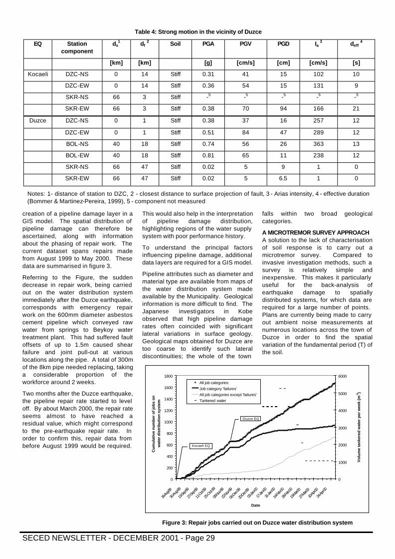
SECED NEWSLETTER - DECEMBER 2001 - Page 29
creation of a pipeline damage layer in a GIS model. The spatial distribution of pipeline damage can therefore be ascertained, along with information about the phasing of repair work. The current dataset spans repairs made from August 1999 to May 2000. These data are summarised in figure 3.
Referring to the Figure, the sudden decrease in repair work, being carried out on the water distribution system immediately after the Duzce earthquake, corresponds with emergency repair work on the 600mm diameter asbestos cement pipeline which conveyed raw water from springs to Beykoy water treatment plant. This had suffered fault offsets of up to 1.5m caused shear failure and joint pull-out at various locations along the pipe. A total of 300m of the 8km pipe needed replacing, taking a considerable proportion of the workforce around 2 weeks.
Two months after the Duzce earthquake, the pipeline repair rate started to level off. By about March 2000, the repair rate seems almost to have reached a residual value, which might correspond to the pre-earthquake repair rate. In order to confirm this, repair data from before August 1999 would be required.
This would also help in the interpretation of pipeline damage distribution, highlighting regions of the water supply system with poor performance history.
To understand the principal factors influencing pipeline damage, additional data layers are required for a GIS model.
Pipeline attributes such as diameter and material type are available from maps of the water distribution system made available by the Municipality. Geological information is more difficult to find. The Japanese investigators in Kobe observed that high pipeline damage rates often coincided with significant lateral variations in surface geology. Geological maps obtained for Duzce are too coarse to identify such lateral discontinuities; the whole of the town
falls within two broad geological categories.
A MICROTREMOR SURVEY APPROACH A solution to the lack of characterisation of soil response is to carry out a microtremor survey. Compared to invasive investigation methods, such a survey is relatively simple and inexpensive. This makes it particularly useful for the back-analysis of earthquake damage to spatially distributed systems, for which data are required for a large number of points. Plans are currently being made to carry out ambient noise measurements at numerous locations across the town of Duzce in order to find the spatial variation of the fundamental period (T) of the soil.
Table 4: Strong motion in the vicinity of Duzce
EQ Station component
ds1 df
2 Soil PGA PGV PGD Ia 3 deff
4
[km] [km] [g] [cm/s] [cm] [cm/s] [s]
Kocaeli DZC-NS 0 14 Stiff 0.31 41 15 102 10
DZC-EW 0 14 Stiff 0.36 54 15 131 9
SKR-NS 66 3 Stiff -5 -5 -5 -5 -5
SKR-EW 66 3 Stiff 0.38 70 94 166 21
Duzce DZC-NS 0 1 Stiff 0.38 37 16 257 12
DZC-EW 0 1 Stiff 0.51 84 47 289 12
BOL-NS 40 18 Stiff 0.74 56 26 363 13
BOL-EW 40 18 Stiff 0.81 65 11 238 12
SKR-NS 66 47 Stiff 0.02 5 9 1 0
SKR-EW 66 47 Stiff 0.02 5 6.5 1 0
Notes: 1- distance of station to DZC, 2 - closest distance to surface projection of fault, 3 - Arias intensity, 4 - effective duration (Bommer & Martinez-Pereira, 1999), 5 - component not measured
0
200
400
600
800
1000
1200
1400
1600
1800
16-Au
g-99
30-Au
g-99
13-Se
p-99
27-Se
p-99
11-Oct-9
9
25-O
ct-99
08-No
v-99
22-No
v-99
06-De
c-99
20-De
c-99
03-Jan
-00
17-Jan
-00
31-Jan
-00
14-Fe
b-00
28-Fe
b-00
13-Mar-0
0
27-Mar-0
0
10-Ap
r-00
24-Ap
r-00
Date
Cu
mu
lativ
e n
um
ber
of j
ob
s o
n
wat
er d
istr
ibu
tion
sys
tem
0
1000
2000
3000
4000
5000
6000
Vol
ume
tank
ered
wat
er p
er w
eek
(m3 )
All job categoriesJob category 'failures'All job categories except 'failures'Tankered water
Kocaeli EQ
Duzce EQ
Figure 3: Repair jobs carried out on Duzce water distribution system
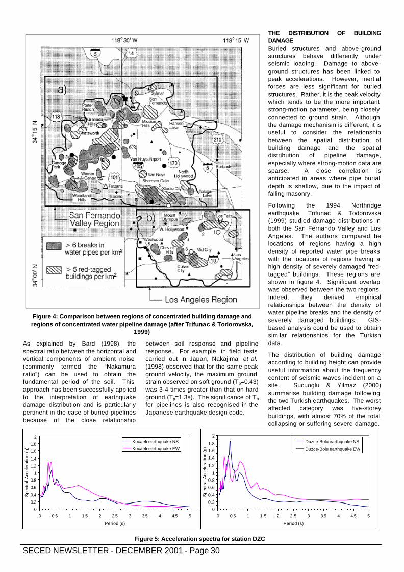
SECED NEWSLETTER - DECEMBER 2001 - Page 30
As explained by Bard (1998), the spectral ratio between the horizontal and vertical components of ambient noise (commonly termed the “Nakamura ratio”) can be used to obtain the fundamental period of the soil. This approach has been successfully applied to the interpretation of earthquake damage distribution and is particularly pertinent in the case of buried pipelines because of the close relationship
between soil response and pipeline response. For example, in field tests carried out in Japan, Nakajima et al. (1998) observed that for the same peak ground velocity, the maximum ground strain observed on soft ground (Tp=0.43) was 3-4 times greater than that on hard ground (Tp=1.3s). The significance of Tp for pipelines is also recognised in the Japanese earthquake design code.
THE DISTRIBUTION OF BUILDING DAMAGE Buried structures and above-ground structures behave differently under seismic loading. Damage to above-ground structures has been linked to peak accelerations. However, inertial forces are less significant for buried structures. Rather, it is the peak velocity which tends to be the more important strong-motion parameter, being closely connected to ground strain. Although the damage mechanism is different, it is useful to consider the relationship between the spatial distribution of building damage and the spatial distribution of pipeline damage, especially where strong-motion data are sparse. A close correlation is anticipated in areas where pipe burial depth is shallow, due to the impact of falling masonry.
Following the 1994 Northridge earthquake, Trifunac & Todorovska (1999) studied damage distributions in both the San Fernando Valley and Los Angeles. The authors compared the locations of regions having a high density of reported water pipe breaks with the locations of regions having a high density of severely damaged “red-tagged” buildings. These regions are shown in figure 4. Significant overlap was observed between the two regions. Indeed, they derived empirical relationships between the density of water pipeline breaks and the density of severely damaged buildings. GIS-based analysis could be used to obtain similar relationships for the Turkish data.
The distribution of building damage according to building height can provide useful information about the frequency content of seismic waves incident on a site. Sucuoglu & Yilmaz (2000) summarise building damage following the two Turkish earthquakes. The worst affected category was five-storey buildings, with almost 70% of the total collapsing or suffering severe damage.
Figure 4: Comparison between regions of concentrated building damage and regions of concentrated water pipeline damage (after Trifunac & Todorovska,
1999)
0
0.2
0.4
0.6
0.8
1
1.2
1.4
1.6
1.8
2
0 0.5 1 1.5 2 2.5 3 3.5 4 4.5 5
Period (s)
Spe
ctra
l Acc
eler
atio
n (g
)
Kocaeli earthquake NS
Kocaeli earthquake EW
0
0.2
0.4
0.6
0.8
1
1.2
1.4
1.6
1.8
2
0 0.5 1 1.5 2 2.5 3 3.5 4 4.5 5
Period (s)
Spe
ctra
l Acc
eler
atio
n (g
)
Duzce-Bolu earthquake NS
Duzce-Bolu earthquake EW
Figure 5: Acceleration spectra for station DZC
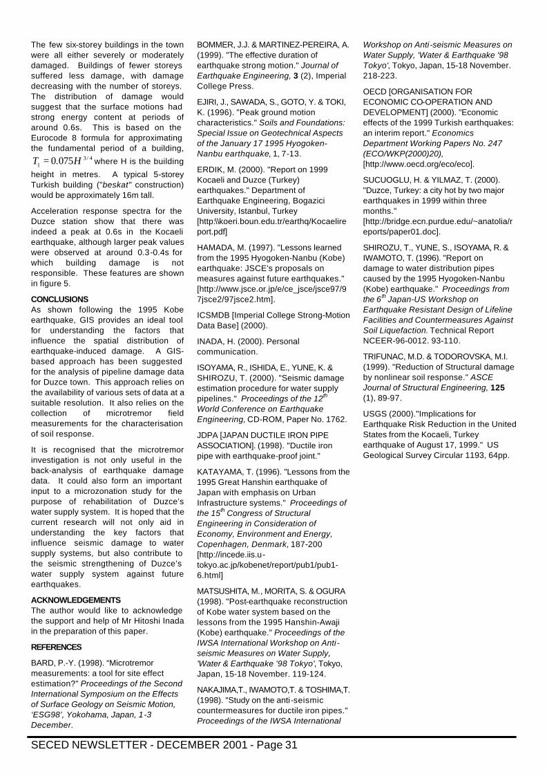
SECED NEWSLETTER - DECEMBER 2001 - Page 31
The few six-storey buildings in the town were all either severely or moderately damaged. Buildings of fewer storeys suffered less damage, with damage decreasing with the number of storeys. The distribution of damage would suggest that the surface motions had strong energy content at periods of around 0.6s. This is based on the Eurocode 8 formula for approximating the fundamental period of a building,
4/31 075.0 HT = where H is the building
height in metres. A typical 5-storey Turkish building ("beskat" construction) would be approximately 16m tall.
Acceleration response spectra for the Duzce station show that there was indeed a peak at 0.6s in the Kocaeli earthquake, although larger peak values were observed at around 0.3-0.4s for which building damage is not responsible. These features are shown in figure 5.
CONCLUSIONS As shown following the 1995 Kobe earthquake, GIS provides an ideal tool for understanding the factors that influence the spatial distribution of earthquake-induced damage. A GIS-based approach has been suggested for the analysis of pipeline damage data for Duzce town. This approach relies on the availability of various sets of data at a suitable resolution. It also relies on the collection of microtremor field measurements for the characterisation of soil response.
It is recognised that the microtremor investigation is not only useful in the back-analysis of earthquake damage data. It could also form an important input to a microzonation study for the purpose of rehabilitation of Duzce’s water supply system. It is hoped that the current research will not only aid in understanding the key factors that influence seismic damage to water supply systems, but also contribute to the seismic strengthening of Duzce’s water supply system against future earthquakes.
ACKNOWLEDGEMENTS The author would like to acknowledge the support and help of Mr Hitoshi Inada in the preparation of this paper.
REFERENCES
BARD, P.-Y. (1998). “Microtremor measurements: a tool for site effect estimation?” Proceedings of the Second International Symposium on the Effects of Surface Geology on Seismic Motion, ‘ESG98’, Yokohama, Japan, 1-3 December.
BOMMER, J.J. & MARTINEZ-PEREIRA, A. (1999). "The effective duration of earthquake strong motion." Journal of Earthquake Engineering, 3 (2), Imperial College Press.
EJIRI, J., SAWADA, S., GOTO, Y. & TOKI, K. (1996). "Peak ground motion characteristics." Soils and Foundations: Special Issue on Geotechnical Aspects of the January 17 1995 Hyogoken-Nanbu earthquake, 1, 7-13.
ERDIK, M. (2000). "Report on 1999 Kocaeli and Duzce (Turkey) earthquakes." Department of Earthquake Engineering, Bogazici University, Istanbul, Turkey [http:\\koeri.boun.edu.tr/earthq/Kocaelireport.pdf]
HAMADA, M. (1997). "Lessons learned from the 1995 Hyogoken-Nanbu (Kobe) earthquake: JSCE's proposals on measures against future earthquakes." [http://www.jsce.or.jp/e/ce_jsce/jsce97/97jsce2/97jsce2.htm].
ICSMDB [Imperial College Strong-Motion Data Base] (2000).
INADA, H. (2000). Personal communication.
ISOYAMA, R., ISHIDA, E., YUNE, K. & SHIROZU, T. (2000). "Seismic damage estimation procedure for water supply pipelines." Proceedings of the 12th World Conference on Earthquake Engineering, CD-ROM, Paper No. 1762.
JDPA [JAPAN DUCTILE IRON PIPE ASSOCIATION]. (1998). "Ductile iron pipe with earthquake-proof joint."
KATAYAMA, T. (1996). "Lessons from the 1995 Great Hanshin earthquake of Japan with emphasis on Urban Infrastructure systems." Proceedings of the 15th Congress of Structural Engineering in Consideration of Economy, Environment and Energy, Copenhagen, Denmark, 187-200 [http://incede.iis.u-tokyo.ac.jp/kobenet/report/pub1/pub1-6.html]
MATSUSHITA, M., MORITA, S. & OGURA (1998). "Post-earthquake reconstruction of Kobe water system based on the lessons from the 1995 Hanshin-Awaji (Kobe) earthquake." Proceedings of the IWSA International Workshop on Anti-seismic Measures on Water Supply, 'Water & Earthquake '98 Tokyo', Tokyo, Japan, 15-18 November. 119-124.
NAKAJIMA,T., IWAMOTO,T. & TOSHIMA,T. (1998). "Study on the anti-seismic countermeasures for ductile iron pipes." Proceedings of the IWSA International
Workshop on Anti-seismic Measures on Water Supply, 'Water & Earthquake '98 Tokyo', Tokyo, Japan, 15-18 November. 218-223.
OECD [ORGANISATION FOR ECONOMIC CO-OPERATION AND DEVELOPMENT] (2000). "Economic effects of the 1999 Turkish earthquakes: an interim report." Economics Department Working Papers No. 247 (ECO/WKP(2000)20), [http://www.oecd.org/eco/eco].
SUCUOGLU, H. & YILMAZ, T. (2000). "Duzce, Turkey: a city hot by two major earthquakes in 1999 within three months." [http://bridge.ecn.purdue.edu/~anatolia/reports/paper01.doc].
SHIROZU, T., YUNE, S., ISOYAMA, R. & IWAMOTO, T. (1996). "Report on damage to water distribution pipes caused by the 1995 Hyogoken-Nanbu (Kobe) earthquake." Proceedings from the 6 th Japan-US Workshop on Earthquake Resistant Design of Lifeline Facilities and Countermeasures Against Soil Liquefaction. Technical Report NCEER-96-0012. 93-110.
TRIFUNAC, M.D. & TODOROVSKA, M.I. (1999). "Reduction of Structural damage by nonlinear soil response." ASCE Journal of Structural Engineering, 125 (1), 89-97.
USGS (2000)."Implications for Earthquake Risk Reduction in the United States from the Kocaeli, Turkey earthquake of August 17, 1999." US Geological Survey Circular 1193, 64pp.

SECED NEWSLETTER - DECEMBER 2001 - Page 32
In-situ and laboratory testing to provide the properties of foundation materials for seismically loaded structures Nick Ramsey of Fugro Ltd outlines and discusses the determination of the soil and rock properties. Properties required Material properties required for seismic analysis are:
• Density • Seismic wave velocities • Dynamic moduli • Poisson’s ratio • Elastic damping
Merits of in-situ and laboratory techniques
In-situ techniques may be used to provide soil properties for seismic analysis.
Advantages: • They provide data on the macro
behaviour of the soil. • They provide accurate estimates of
G0 Disadvantages: • They do not provide information on
the behaviour of soil at higher strain levels
• They do not provide information on soil damping
Laboratory techniques are preferably used to supplement in-situ test data.
Advantages: • Changes in stiffness, damping and
pore water associated with strain levels can be assessed
• Soil samples can be reconsolidated to take account of the increase in stresses caused by the structural loading
• Tests are performed in a controlled environment
Disadvantages:
• In sandy soils in particular the method of preparation can affect the soil response.
• A much smaller amount of soil is being tested so macro effects may not be apparent
• The 3-dimensional nature of an earthquake is not taken into account
Since the effects of competent rock depends upon flaws and discontinuities it is essential that every effort is made to determine their nature, extent and orientation by whatever means is available.
Methods of assessing dynamic moduli
In-situ tests: • Cross-hole seismic testing. • Seismic cone testing. • Pressuremeter testing.
Laboratory tests: • Bender element tests are used to
assess shear wave velocity and G0.
• Local strain measurements are used to assess soil stiffness and Poisson’s ratio.
• Resonant column tests are used to assess G0 and stiffness degradation.
• Stress-controlled cyclic simple shear and cyclic triaxial tests are used to assess stiffness degradation and liquefaction potential as a function of number of cycles of applied loading.
• Strain-controlled cyclic simple shear and cyclic triaxial tests are used to assess hysteretic damping.
Recommended approach
In soil: • Assess whether a refined
computer model may be justified. • Use field tests to provide reference
values for in-situ stiffness. • Use bender element and resonant
column tests to assess Gmax. • Use local strain measurements to
assess Poisson’s ratio and stiffness degradation.
• Use resonant column and strain-controlled cyclic tests to assess dynamic moduli and damping.
• Use stress-controlled cyclic tests to assess effective stresses and liquefaction potential.
In rock: • The depth may limit the options
available, but both in-situ and laboratory techniques may be used.
• Outcrops, geological records and GIS, indicate where investigations are likely to be most profitable.
SECED Newsletter The SECED Newsletter is published quarterly. Contributions are welcome and manuscripts should be sent on a PC compatible disk or directly by Email. Copy typed on one side of the paper only is also acceptable.
Diagrams should be sharply defined and prepared in a form suitable for direct reproduction. Photographs should be high quality (black and white prints are preferred). Diagrams and photographs are only returned to the authors on request. Diagrams and pictures may also be sent by Email (GIF format is preferred).
Articles should be sent to:
Adam Crewe, Editor SECED Newsletter, University of Bristol, Department of Civil Engineering, Queen’s Building, University Walk, Bristol BS8 1TR, UK.
Email: [email protected]
SECED SECED, The Society for Earthquake and Civil Engineering Dynamics, is the UK national section of the International and European Associations for Earthquake Engineering and is an affiliated society of the Institution of Civil Engineers.
It is also sponsored by the Institution of Mechanical Engineers, the Institution of Structural Engineers, and the Geophysical Society. The Society is also closely associated with the UK Earthquake Engineering Field Investigation Team. The objective of the Society is to promote co-operation in the advancement of knowledge in the fields of earthquake engineering and civil engineering dynamics including blast, impact and other vibration problems.
For further information about SECED contact: The Secretary, SECED, Institution of Civil Engineers, Great George Street, London SW1P 3AA, UK.
Special Issue Contents Introduction Page 1
Observed damage to buried structures
Page 2
Seismic effects on immersed tube tunnels
Page 4
Design of tunnels for earthquake ground motions
Page 9
On shaky ground Page 14
Caverns in earthquakes Page 21
Behaviour of water distribution pipelines
Page 26
In-situ testing to determine soil and rock properties
Page 32