1

Seasonal Volatility of Corn Futures Prices*†‡

Caleb Seeley

Fall 2009

___________________________

* This report was completed in compliance with the Duke Community Standard † Professor George Tauchen, Faculty Advisor

‡ Honors Thesis submitted in partial fulfillment of the requirements for Graduation with Distinction in

Economics in Trinity College of Duke University

2

Abstract

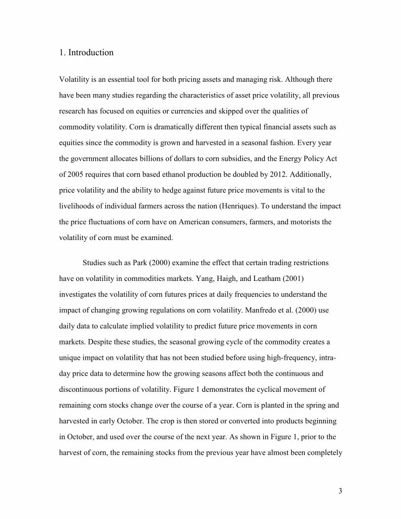
This paper examines the seasonal patterns evident in the volatility of corn futures

prices. It adds to the high-frequency volatility literature by exploring large price

discontinuities (jumps), and both the continuous and discontinuous portions of volatility

in a commodity, corn. Furthermore, the paper analyzes how the growing cycle of corn

influences volatility over the course of a year. After identifying a distinct pattern in the

volatility of corn over the growing season, this paper articulates some of the potential

causes of the observed trend. The amount of information available to the market seems to

drive the volatility of corn prices, and the changes in volatility occur almost entirely in

the continuous portion of volatility which led to jumps being evenly distributed

throughout the year.

3

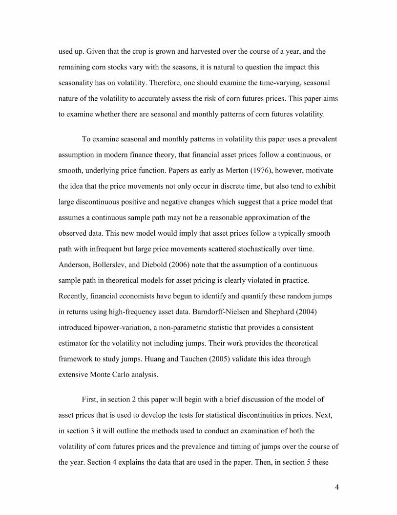
1. Introduction

Volatility is an essential tool for both pricing assets and managing risk. Although there

have been many studies regarding the characteristics of asset price volatility, all previous

research has focused on equities or currencies and skipped over the qualities of

commodity volatility. Corn is dramatically different then typical financial assets such as

equities since the commodity is grown and harvested in a seasonal fashion. Every year

the government allocates billions of dollars to corn subsidies, and the Energy Policy Act

of 2005 requires that corn based ethanol production be doubled by 2012. Additionally,

price volatility and the ability to hedge against future price movements is vital to the

livelihoods of individual farmers across the nation (Henriques). To understand the impact

the price fluctuations of corn have on American consumers, farmers, and motorists the

volatility of corn must be examined.

Studies such as Park (2000) examine the effect that certain trading restrictions

have on volatility in commodities markets. Yang, Haigh, and Leatham (2001)

investigates the volatility of corn futures prices at daily frequencies to understand the

impact of changing growing regulations on corn volatility. Manfredo et al. (2000) use

daily data to calculate implied volatility to predict future price movements in corn

markets. Despite these studies, the seasonal growing cycle of the commodity creates a

unique impact on volatility that has not been studied before using high-frequency, intra-

day price data to determine how the growing seasons affect both the continuous and

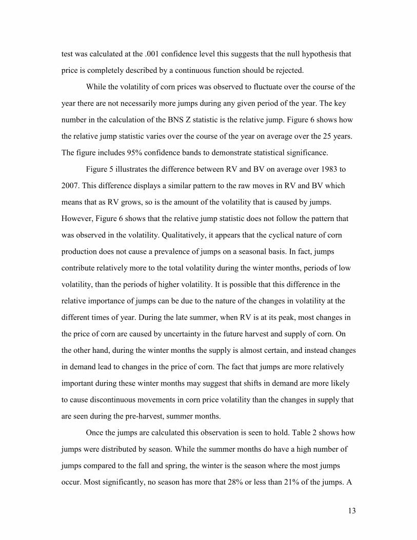
discontinuous portions of volatility. Figure 1 demonstrates the cyclical movement of

remaining corn stocks change over the course of a year. Corn is planted in the spring and

harvested in early October. The crop is then stored or converted into products beginning

in October, and used over the course of the next year. As shown in Figure 1, prior to the

harvest of corn, the remaining stocks from the previous year have almost been completely

4

used up. Given that the crop is grown and harvested over the course of a year, and the

remaining corn stocks vary with the seasons, it is natural to question the impact this

seasonality has on volatility. Therefore, one should examine the time-varying, seasonal

nature of the volatility to accurately assess the risk of corn futures prices. This paper aims

to examine whether there are seasonal and monthly patterns of corn futures volatility.

To examine seasonal and monthly patterns in volatility this paper uses a prevalent

assumption in modern finance theory, that financial asset prices follow a continuous, or

smooth, underlying price function. Papers as early as Merton (1976), however, motivate

the idea that the price movements not only occur in discrete time, but also tend to exhibit

large discontinuous positive and negative changes which suggest that a price model that

assumes a continuous sample path may not be a reasonable approximation of the

observed data. This new model would imply that asset prices follow a typically smooth

path with infrequent but large price movements scattered stochastically over time.

Anderson, Bollerslev, and Diebold (2006) note that the assumption of a continuous

sample path in theoretical models for asset pricing is clearly violated in practice.

Recently, financial economists have begun to identify and quantify these random jumps

in returns using high-frequency asset data. Barndorff-Nielsen and Shephard (2004)

introduced bipower-variation, a non-parametric statistic that provides a consistent

estimator for the volatility not including jumps. Their work provides the theoretical

framework to study jumps. Huang and Tauchen (2005) validate this idea through

extensive Monte Carlo analysis.

First, in section 2 this paper will begin with a brief discussion of the model of

asset prices that is used to develop the tests for statistical discontinuities in prices. Next,

in section 3 it will outline the methods used to conduct an examination of both the

volatility of corn futures prices and the prevalence and timing of jumps over the course of

the year. Section 4 explains the data that are used in the paper. Then, in section 5 these

5

results will be analyzed compared to the growing and harvesting pattern of corn in order

to better understand how the seasonal nature of corn production impacts the volatility of

the commodity.

2 Stochastic Model of Returns

It is important to understand the theoretical model of asset price movements and the

concept of market microstructure noise that are used to derive the results of this paper. To

motivate our discussion of jump discontinuities and seasonal volatility in corn futures

prices we will begin by investigating a standard model of asset price evolution. This

paper considers a log price, p(t), that changes over time as

where µ(t)dt represents the time-varying drift component of the asset. The time-varying

volatility of the price movement is represented by σ(t) where the dW(t) term is

standardized Brownian motion. The equation defined above is the continuous time

interpretation of a Binomial model in which the price can either more up or down over

small time intervals. The drift term and the standard Brownian motion are the

consequences of adding independent identically distributed log-returns over

infinitesimally small time periods.

Recent literature has suggested that the addition of jumps in the price process is

important for theoretical and empirical modeling. Merton (1976) introduced the

following equation to include a jump process:

6

where the non-continuous portion of the price movement is added with the term κ(t)dq(t).

In this equation q(t) is a counting process and k(t) is the magnitude of the jump. Here,

while the price paths still take place in continuous time, the paths are discontinuous.

3. Methods

To determine whether a statistically significant price discontinuity, or jump, occurs

during a trading period, high frequency measures of variance must be calculated.

Barndorff-Nielsen and Shephard (2004) introduced a test that uses high frequency price

data to determine if there is a jump over the course of a day. The test compares two

different measures of variance: realized variance and bipower variation. The variance is

calculated daily in unit t, and intraday geometric returns are defined as

where p is the log price and M is the number of observations in the given day. The first

measure of quadratic variation is the realized variance (RV) which is defined as:

and the alternate measure is realized bipower variation (BV) which is defined:

7

Both of these two measures were thoroughly investigated in Barndorf-Neilsen and

Shephard (2005) to produce asymptotic results that allow for the separate identification of

the continuous and jump components of the quadratic variation. While the RV measures

both the variation of the continuous process and the jump process, the BV only measures

the variation of the continuous process. The BV is robust to jumps because it multiplies

adjacent returns. Thus any singular, large price move will be canceled out when it is

followed or preceded by, and thus multiplied by, a small return. Therefore, the difference

between the RV and the BV isolates the jump component of the daily volatility.

Furthermore, to measure of the percentage of total variance caused by the jump process

this paper uses the relative jump:

This result can be used to test the hypothesis that no jump occurred on any particular day.

The test can be expressed as a z-statistic:

where TP is the tripower quarticity defined as:

The TP is used in this test because, as shown in Barndorf-Nielsen and Shephard (2004), it

converges to the integrated quarticity of the price process. And Huang and Tauchen

(2005) discovered that the best test statistic for jump detection is the Z-Tripower-Max

8

test statistic as represented in equation 5. The statistic, Zt, approaches a standard normal

distribution, N(0, 1), as M approaches infinity and the data get denser.

The test operates under the assumption that there are no jumps. This means that

higher values Z suggest the presence of jumps on a particular day. When Zt is sufficiently

high then we can reject the null hypothesis that there are no jumps. Throughout this

paper, the Z-statistic is tested at the .001 confidence level to distinguish a day with jumps

from a day without jumps.

Another method of computing variance, Realized Semi-Variance, is also

investigated. RS is defined by Barndorff-Nielsen, Kinnebrock, and Shephard (2008) in

order to separate the negative and positive variation. Realized Semi-Variance is the sum

of squared negative returns and for the purposes of this paper will be referred to as down-

variance, DV.

Up-Variance, also developed in the same paper, is the sum of squared positive returns,

but for purposes of simplicity is calculated by:

Realized DV and UV were initially developed to examine the predictive power of

negative and positive returns on volatility, but are used here to examine potential causes

of the trends observed in the seasonal variance of corn futures prices.

4. Data

9

This paper examines the prices of corn futures from the start of trading in January 1983 to

the end of trading in December 2007. The high-frequency corn futures data used for this

research were purchased from http://tickdata.com. The data were delivered in one-minute

intervals, but the returns used in this paper are calculated at five minute intervals in an

attempt to find a balance between the micro-structure noise, and a significant amount of

data. The fundamental value for corn futures is determined by forward-looking supply

and demand. The predicted intersection of supply and demand at the delivery date is

constantly changing. Microstructure-noise results from bid-ask bounce, the time it takes

information to reach the market, and other high-frequency factors that cause the price to

deviate slightly from this fundamental value. Market microstructure noise is noticeable

when estimating variance using high frequency data, and can have a significant impact on

tests for jumps in asset prices.

Corn was chosen for this study since it has a cyclical, seasonal growing pattern,

and is the most widely produced feed grain in the United States, accounting for more than

90 percent of total value and production of feed grains. Around 80 million acres of land

are planted to corn, with the majority of the crop grown in the aptly named Corn Belt.

The Corn Belt includes the states of Michigan, Minnesota, South Dakota, Wisconsin,

Ohio, Illinois, Indiana, Iowa, Missouri, Kansas, and Nebraska. Most of the crop is used as

the main energy ingredient in livestock feed. Hogs, cattle, sheep, and poultry eat more

than half of the corn grain grown each year. Corn is also processed into a multitude of

food and industrial products including starch, sweeteners, corn oil, beverage and

industrial alcohol, and fuel ethanol. Some corn is used for silage. Corn silage is livestock

food that is made from the parts of the corn plant that are left after the roots and ears of

corn have been taken off.

The commodity futures are traded on the Chicago Board of Trade from 9:30 am

to 1:15 pm central time through both open-outcry and, more recently, electronic methods.

10

Each contract is a dollar denominated physical delivery contract of 5000 bushels,

approximately 127 metric tons. The prices are quoted in cents and quarter cents per

bushel. Corn futures provide a way to participate in price discovery, and manage

exposure to price risk for corn producers, food processors, livestock operators, and other

market participants have related to the purchase and sale of corn.

5. Results

The results are split into three sections. First, the trends of both RV and BV are

examined. Next, DV is studied in an attempt to understand potential causes of the trends

observed in the variance. Thirdly, the amount and time of occurrence of jumps is assessed

to further understand the seasonal trends in corn futures price volatility.

5.1 RV and BV

Over the 25 years from which the data were collected, 1983-2007, the RV when

expressed in standard deviation and annualized implies an average annualized volatility

of 17.07%. When BV is expressed in the same manner the implied annualized volatility is

slightly lower at 15.93%. The average volatility of the stock market during this same time

was about 16.00%. This suggests that there are discontinuities in the price moves

throughout each year which are expressed in the RV but not picked up by the BV.

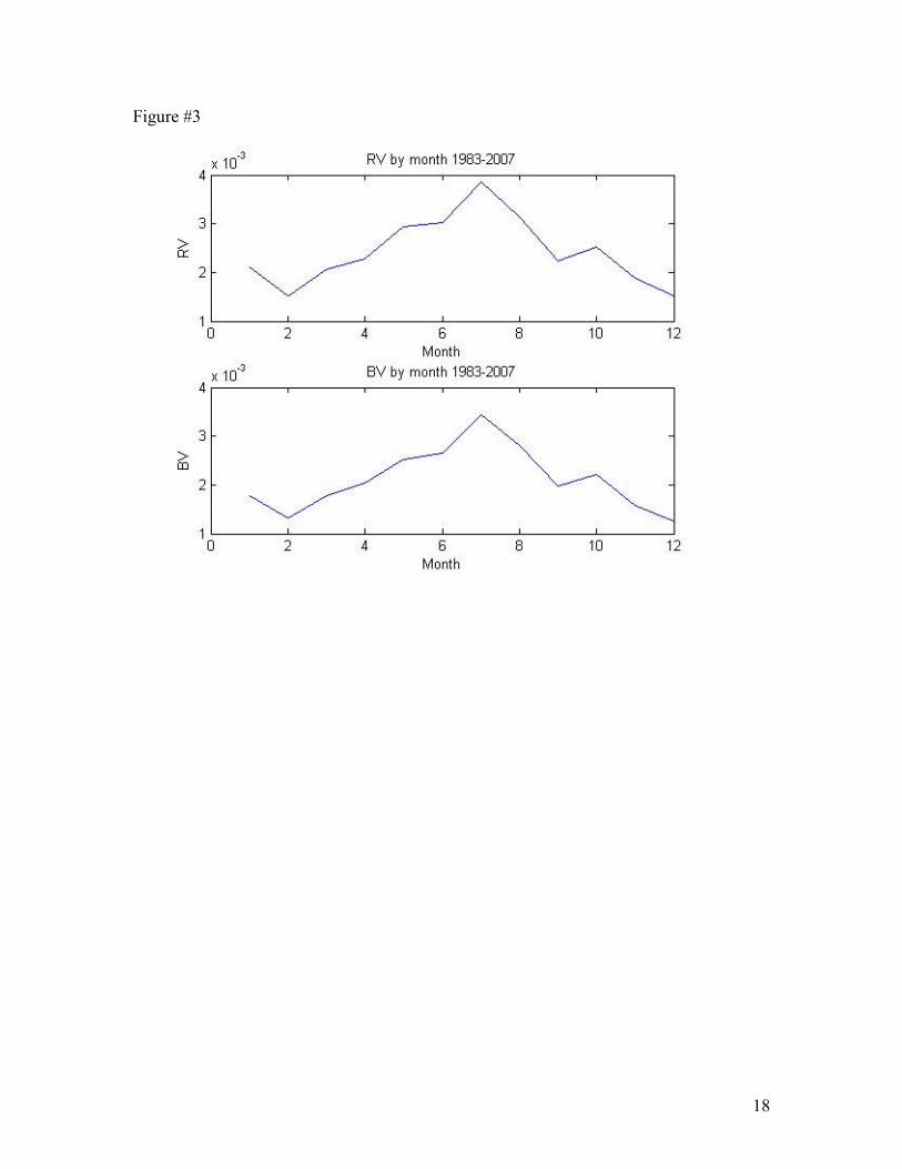
Additionally, the volatility was not constant throughout the year. Figure 3 shows both the

average RV and average BV on a month by month basis over the 25 years. The RV

increases linearly from low volatility in February to a peak in July before decreasing over

the later months of the year.

Remarkably, the remaining corn stocks at the end of each quarter (Figure 1)

follow a striking seasonal pattern that can explain the observed shifts in RV and BV

during the course of a year. Immediately following a harvest, when remaining corn stocks

are at their peak, the volatility of corn prices are at the lowest point, the RV represented

11

as annualized volatility is 13.42%. Right before the harvest, however, with corn stocks at

their lowest level, the volatility of futures prices is at its highest point, the RV implies an

annualized volatility of 21.63%. The difference between the trough of RV and the peak of

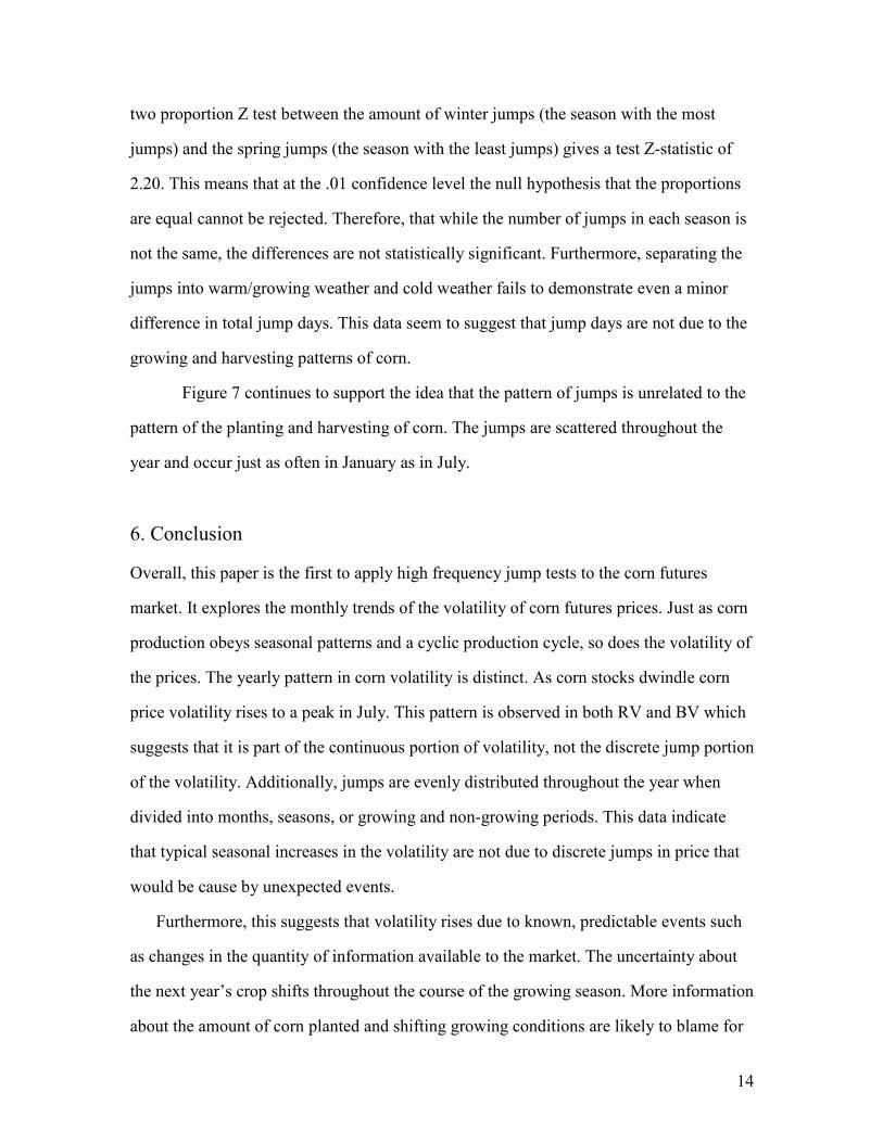
the RV is statistically significant at a .01 level. The disappearance of corn stocks, shown

in Figure 2, follows a similar trend, but the stocks remaining at the end of August are not

enough to sustain the same levels of consumption. Since futures markets are intended to

aid in price discovery, the price seems most volatile when the supply is at a very low

level, and the future supply is not fully known.

The timing of the crop reports released by the USDA provides further evidence

that quantity of information possessed by market participants extensively contributes to

the observed pattern of volatility. At the end of each March (the beginning of corn

growing season) the Prospective Plantings report indicates how many acres of corn

producers are expecting to plant. At precisely this time, the RV and BV begin to increase

as information about the future supply of corn reaches the market. Then, as the summer

progresses, monthly crop production reports are issued to give an updated estimate of the

supply and demand for corn. In June, the USDA releases a more concrete plantings

report, shortly after which the volatility of corn prices reaches its peak. Once this

information about the harvest has been absorbed by the market the volatility begins to

decrease steadily. Finally, after the October harvest there the volatility reaches its lows as

market participants wait until next March for any supply information to be calculated.

Interestingly, the BV also exhibits the same pattern. This suggests that the time

varying nature of the volatility is largely explained by the continuous portion for the price

evolution function. If the seasonal nature of the harvest caused statistically significant

discontinuities in returns then there would be a difference between the patterns of the RV

and the BV over the course of the year. However, when analyzed at either a monthly or

weekly interval, the RV and BV demonstrate the same single peaked pattern over the

course of the year.

12

5.2 Realized Down-Variance

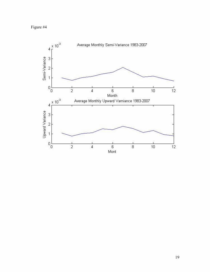
DV can be used to better understand potential causes of the seasonal trend that is

observed in both RV and BV. DV is the variance of only negative returns. If corn price

volatility rises only due to natural disasters or other sudden shocks that unexpectedly hurt

the future supply of corn then there would likely be larger price increases than price

decreases. Thus, DV would be constant throughout the year while UV would display the

same significant single peaked shape that is seen in both the RV and the BV in Figure 3.

However, as seen in Figure 4, this is not the case.

The DV and UV both follow the same pattern as the RV and BV in figure 2. Not

only is this pattern qualitatively the same for RV, BV, DV and UV on a monthly and

weekly interval throughout the year, but also UV is always slightly greater than UV. This

indicates that there is no significant trend in returns that suggests disasters, or other

supply constraining events, are driving the volatility of corn futures prices. If that were

the case, it would be indicated by positive returns dominating negative returns during the

late spring and summer months of each year. This indicates that price shifts occur in both

directions with similar magnitude. Producers can plant more acres than initially expected

just as easily as they may plant fewer acres than were predicted by the USDA surveys.

This supports the idea that the volatility changes of corn futures prices over the course of

each year are largely continuous and not caused by discontinuous price jumps which may

be caused by unexpected supply shocks.

5.3 Jumps

For the entire sample there were 372 total days that were identified by the BNS

test as containing jumps. This is 5.8% of the total number of days in the sample. Since the

13

test was calculated at the .001 confidence level this suggests that the null hypothesis that

price is completely described by a continuous function should be rejected.

While the volatility of corn prices was observed to fluctuate over the course of the

year there are not necessarily more jumps during any given period of the year. The key

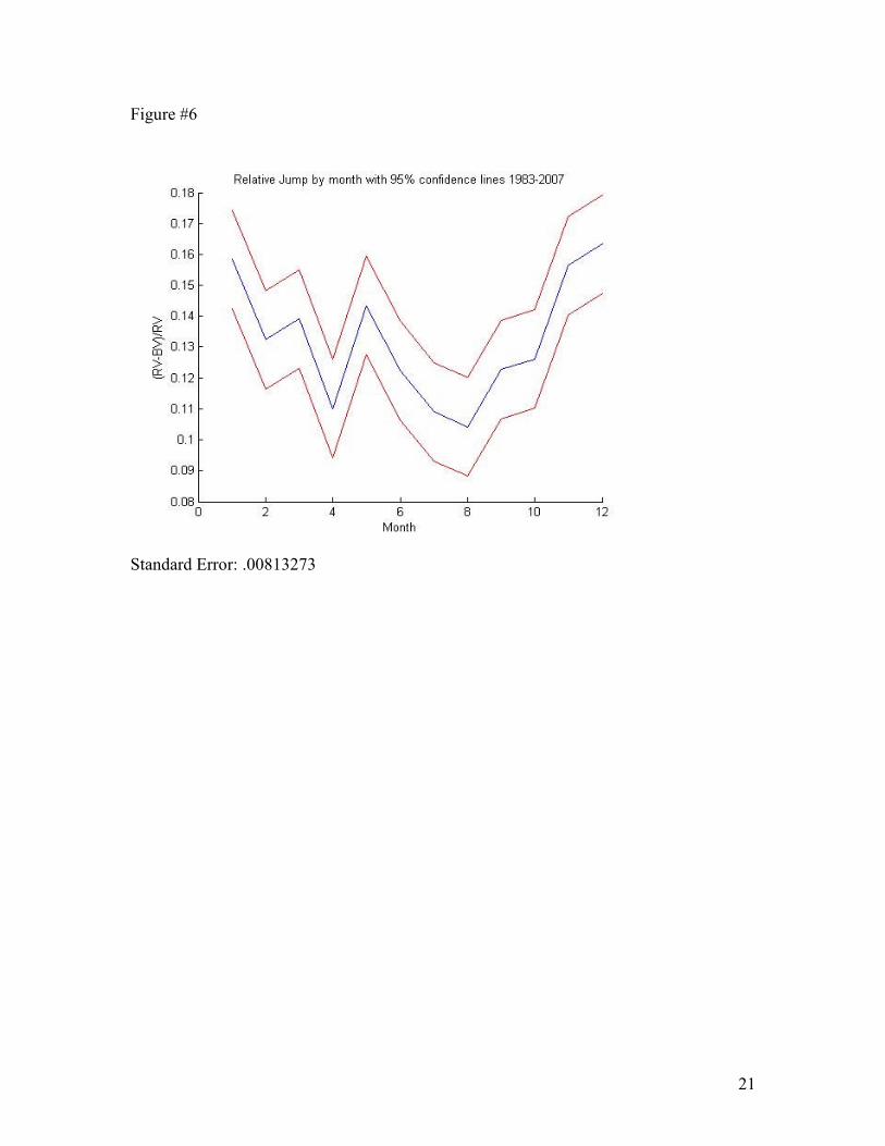
number in the calculation of the BNS Z statistic is the relative jump. Figure 6 shows how

the relative jump statistic varies over the course of the year on average over the 25 years.

The figure includes 95% confidence bands to demonstrate statistical significance.

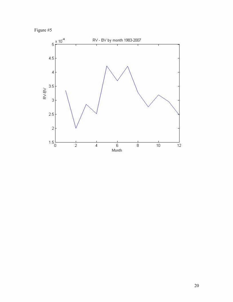
Figure 5 illustrates the difference between RV and BV on average over 1983 to

2007. This difference displays a similar pattern to the raw moves in RV and BV which

means that as RV grows, so is the amount of the volatility that is caused by jumps.

However, Figure 6 shows that the relative jump statistic does not follow the pattern that

was observed in the volatility. Qualitatively, it appears that the cyclical nature of corn

production does not cause a prevalence of jumps on a seasonal basis. In fact, jumps

contribute relatively more to the total volatility during the winter months, periods of low

volatility, than the periods of higher volatility. It is possible that this difference in the

relative importance of jumps can be due to the nature of the changes in volatility at the

different times of year. During the late summer, when RV is at its peak, most changes in

the price of corn are caused by uncertainty in the future harvest and supply of corn. On

the other hand, during the winter months the supply is almost certain, and instead changes

in demand lead to changes in the price of corn. The fact that jumps are more relatively

important during these winter months may suggest that shifts in demand are more likely

to cause discontinuous movements in corn price volatility than the changes in supply that

are seen during the pre-harvest, summer months.

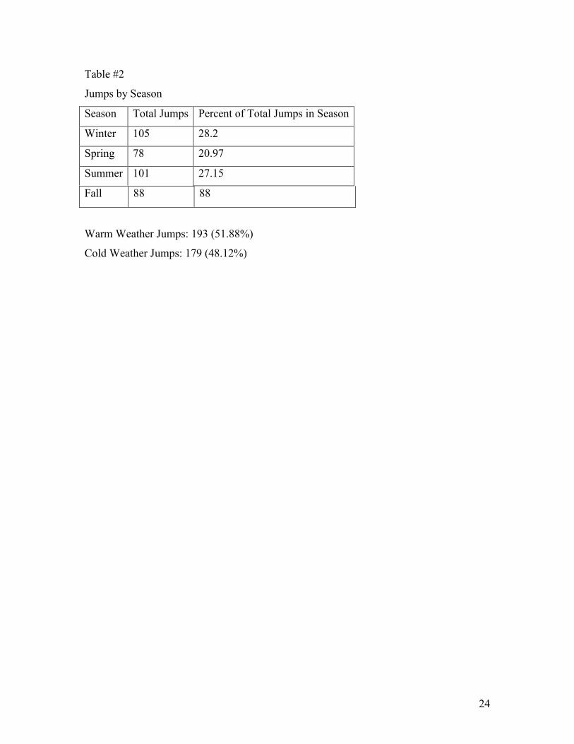
Once the jumps are calculated this observation is seen to hold. Table 2 shows how

jumps were distributed by season. While the summer months do have a high number of

jumps compared to the fall and spring, the winter is the season where the most jumps

occur. Most significantly, no season has more that 28% or less than 21% of the jumps. A

14

two proportion Z test between the amount of winter jumps (the season with the most

jumps) and the spring jumps (the season with the least jumps) gives a test Z-statistic of

2.20. This means that at the .01 confidence level the null hypothesis that the proportions

are equal cannot be rejected. Therefore, that while the number of jumps in each season is

not the same, the differences are not statistically significant. Furthermore, separating the

jumps into warm/growing weather and cold weather fails to demonstrate even a minor

difference in total jump days. This data seem to suggest that jump days are not due to the

growing and harvesting patterns of corn.

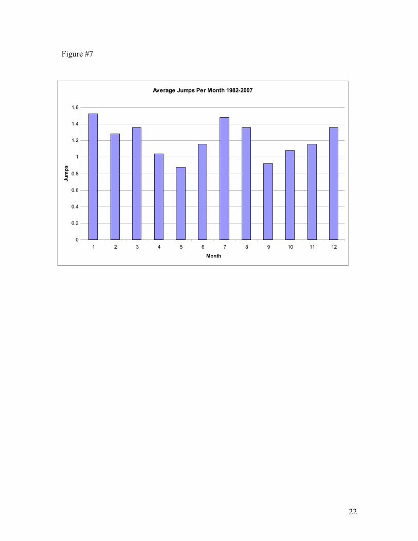
Figure 7 continues to support the idea that the pattern of jumps is unrelated to the

pattern of the planting and harvesting of corn. The jumps are scattered throughout the

year and occur just as often in January as in July.

6. Conclusion

Overall, this paper is the first to apply high frequency jump tests to the corn futures

market. It explores the monthly trends of the volatility of corn futures prices. Just as corn

production obeys seasonal patterns and a cyclic production cycle, so does the volatility of

the prices. The yearly pattern in corn volatility is distinct. As corn stocks dwindle corn

price volatility rises to a peak in July. This pattern is observed in both RV and BV which

suggests that it is part of the continuous portion of volatility, not the discrete jump portion

of the volatility. Additionally, jumps are evenly distributed throughout the year when

divided into months, seasons, or growing and non-growing periods. This data indicate

that typical seasonal increases in the volatility are not due to discrete jumps in price that

would be cause by unexpected events.

Furthermore, this suggests that volatility rises due to known, predictable events such

as changes in the quantity of information available to the market. The uncertainty about

the next year’s crop shifts throughout the course of the growing season. More information

about the amount of corn planted and shifting growing conditions are likely to blame for

15

increases in volatility. Neither natural disasters nor large unexpected shifts in the size of

the harvest are to blame for the rise in volatility. This explains why the continuous

volatility increases as corn stocks dwindle, and follows a distinct seasonal pattern in line

with the cyclical production cycle of the commodity.

16

A. Figures

Figure #1

Ending Corn Stocks

0.00

2,000.00

4,000.00

6,000.00

8,000.00

10,000.00

12,000.00

Sept.-Nov. Dec.-Feb. Mar.-May Jun.-Aug.

Quarter

Millions of Bushels 2001

2002

2003

2004

2005

2006

17

Figure #2

Total Corn Disappearance

0.00

500.00

1,000.00

1,500.00

2,000.00

2,500.00

3,000.00

3,500.00

4,000.00

Sept.-Nov. Dec.-Feb. Mar.-May Jun.-Aug.

Quarter

Millions o

f Bushels 2001

2002

2003

2004

2005

2006

18

Figure #3

19

Figure #4

20

Figure #5

21

Figure #6

Standard Error: .00813273

22

Figure #7

Average Jumps Per Month 1982-2007

0

0.2

0.4

0.6

0.8

1

1.2

1.4

1.6

1 2 3 4 5 6 7 8 9 10 11 12

Month

Jumps

23

B. Tables

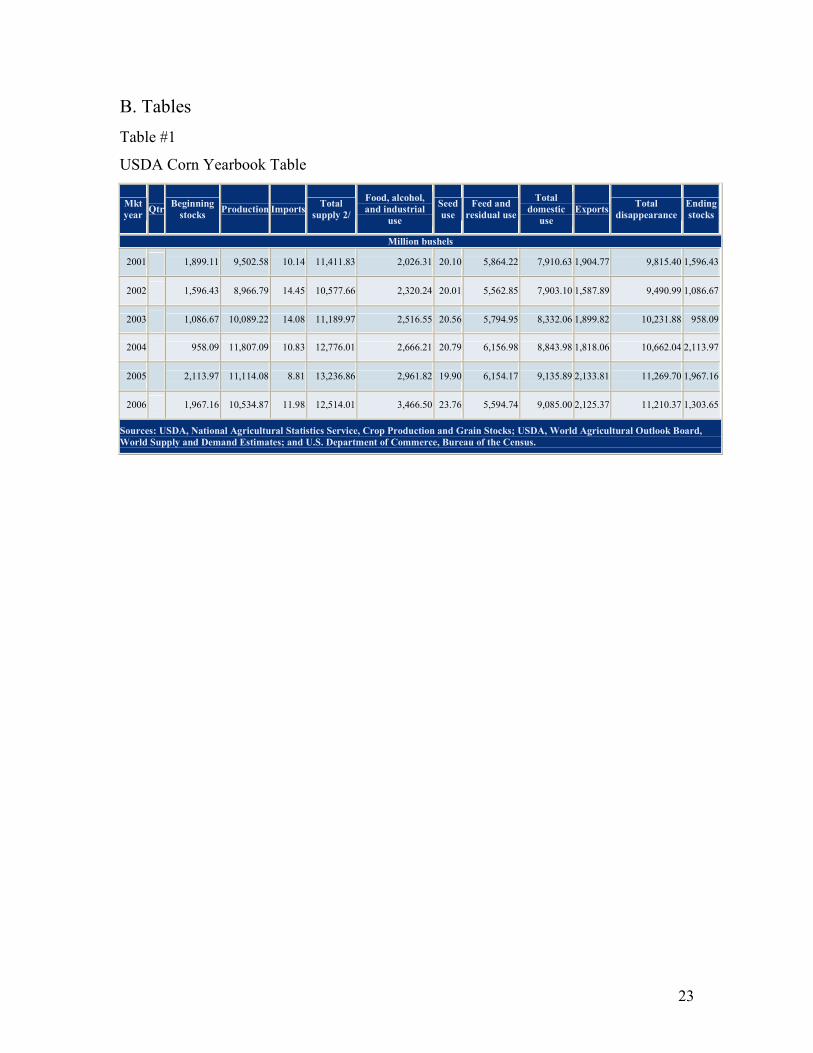
Table #1

USDA Corn Yearbook Table

Mkt

year Qtr Beginning stocks Production Imports Total

supply 2/ Food, alcohol,

and industrial

use Seed

use Feed and

residual use Total

domestic

use Exports Total

disappearance Ending

stocks

Million bushels

2001 1,899.11 9,502.58 10.14 11,411.83 2,026.31 20.10 5,864.22 7,910.63 1,904.77 9,815.40 1,596.43

2002 1,596.43 8,966.79 14.45 10,577.66 2,320.24 20.01 5,562.85 7,903.10 1,587.89 9,490.99 1,086.67

2003 1,086.67 10,089.22 14.08 11,189.97 2,516.55 20.56 5,794.95 8,332.06 1,899.82 10,231.88 958.09

2004 958.09 11,807.09 10.83 12,776.01 2,666.21 20.79 6,156.98 8,843.98 1,818.06 10,662.04 2,113.97

2005 2,113.97 11,114.08 8.81 13,236.86 2,961.82 19.90 6,154.17 9,135.89 2,133.81 11,269.70 1,967.16

2006 1,967.16 10,534.87 11.98 12,514.01 3,466.50 23.76 5,594.74 9,085.00 2,125.37 11,210.37 1,303.65

Sources: USDA, National Agricultural Statistics Service, Crop Production and Grain Stocks; USDA, World Agricultural Outlook Board,

World Supply and Demand Estimates; and U.S. Department of Commerce, Bureau of the Census.

24

Table #2

Jumps by Season

Season Total Jumps Percent of Total Jumps in Season

Winter 105 28.2

Spring 78 20.97

Summer 101 27.15

Fall 88 88

Warm Weather Jumps: 193 (51.88%)

Cold Weather Jumps: 179 (48.12%)

25

8. References

Allen, Edward and Allen Baker, 2005, “Feed Outlook”. FDS-05j, USDA, Economic

Research Service, November 2005

Andersen, T. G., Bollerslev, T., and Diebold, F. X. (2006), “Roughing it Up: Including

Jump Components in the Measurement, Modeling and Forecasting of Return

Volatility.” The Review of Economics and Statistics, 89(4): 701-720.

Barndorff-Nielsen, O.E., and N. Shephard, 2004, “Power and Bipower Variation with

Stochastic Volatility and Jumps.” Journal of Financial Econometrics 2, 1-48.

Barndorff-Nielsen, Ole E., Svend Erik Graversen, Jean Jacod, Mark Podolskij, and Neil

Shephard. (2006). “Econometrics of Testing for Jumps in Financial Economics

Using Bipower Variation. Journal of Financial Econometrics, 4, 1-30.

Barndorf-Nielsen, Ole E, Silja Kinnebrock and Neil Shephard (2008). “Measuring

Downside Risk – Realized Semi-Variance”

“Corn Production Supply and Distribution” 2008. United States Department of

Agriculture. March 15 2008. http://www.fas.usda.gov/psdonline/

Henriques. Diana B. "Price Volatility Adds to Worry on U.S. Farms," New York

TimesWorry on U.S. Farms 22/04/2008. 3 Dec 2008

<http://www.nytimes.com/2008/04/22/business/22commodity.html>

Huang, X. and G. Tauchen, 2005, “The Relative Contribution of Jumps to Total Price

Variance,” Journal of Financial Econometrics 3, 456-499.

Manfredo, Mark R., Leuthold, Raymond M. and Irwin, Scott H.. “Forecasting Cash Price

Volatility of Fed Cattle, Feeder Cattle, and Corn: Time Series, Implied Volatility,

and Composite Approaches”. OFOR Working Paper No. 99-08.

Merton, R.C. (1971). “Optimum Consumption and Portfolio Rules in a Continuous-Time

Model”. Journal of Economic Theory, 3, 373-413.

Merton, R.C. (1976). “The Impact on Option Pricing of Specification Error in the

Underlying Stock Price Returns”. Journal of Finance, 31, 333-350.

Park, Chul Woo. "Examining futures price changes and volatility on the trading day after

a limit-lock day." Journal of Futures Markets 20(2000): 445-466.

26

Van Tassel, P. (2008). “Patterns within the Trading Day: Volatility and Jump

Discontinuities in High Frequency Equity Price Series”. Duke Journal of

Economics, Undergraduate Research Symposium Spring 2008.

Yang, Jian; Haigh, Michael S.; Leatham, David J.. "Agricultural liberalization policy and

commodity price volatility: a GARCH application" Applied Economics Letters

8.9 (2001). 04 Dec. 2008