Seasonal Variations of Hydrological Influences · Seasonal Variations of Hydrological Influences ... their state of weathering and tectonic influences (formation of clefts and cavities

Seasonal Variations of Hydrological Influences

on Gravity Measurements at Wettzell

Martina Harnisch, Günter Harnischformerly Bundesamt für Kartographie und Geodäsie (BKG)

Richard-Strauss-Allee 11, D-60598 Frankfurt am Main

1. IntroductionDuring the first years of gravimeter recordings at Wettzell hydrological influences were assumed to be unimportant.Arguments were: station on a mountain top, rocky underground, water circulation only in clefts etc. However, at leastsince R. FALK [7] found a clear correlation between absolute gravity measurements and groundwater, there is no doubtabout the presence of hydrological influences on the gravity at Wettzell (fig. 1). If the influence of groundwater variationsis corrected, the scattering range of the measured absolute values decreases from more than 100 nm s‑2 to about 50nm s‑2, which much better corresponds to the expected accuracy of the FG5.

Fig. 1: Correlation between changes of the groundwater level and gravity variations, measured with the absolutegravimeter FG5-101 at Wettzell.

The changes of the groundwater level at Wettzell may reach about 4 m (fig. 2). The formal fit of a sinusoidal wave with aperiod of 365.25 days to the groundwater data results in an amplitude of 57.02 cm. Using a groundwater regressioncoefficient of 0.689 nm s-2/cm (the value which was derived from the comparisons with absolute gravity measurements),the corresponding gravity variations would be near ±40 nm s-2. It is clear that variations of such an amount are verydangerous for investigations of long-term gravity phenomena and that they must be taken into account and eliminatedvery carefully.

Seasonal Variations of Hydrological Influences http://www.upf.pf/ICET/bim/text/harnisch2.htm

1 of 13 2/22/2011 9:40 AM

Fig. 2: Long-term changes of the groundwater level at Wettzell and the corresponding annual gravity variations.

2. Some problems of hydrological modeling in gravimetryThe infiltration of water into the underground and its redistribution are very complex processes. Because of the greateconomical importance there are many attempts of hydrological modeling, which aim at the estimation of waterresources. Generally the fundamental equation of hydrology (equation of the water balance) is valid

P = R0 + E + (A – C)

(1)

where P = precipitation, R0 = run-off at the earth’s surface, E = evaporation, A = accumulation (= increase of water in acertain area during a certain time) and C = consumption (= decrease of water in a certain area during a certain time).Each of the constituents of this equation may be influenced by different factors in different ways.First of all the accumulation of water depends on the rocks in the underground, their state of weathering and tectonicinfluences (formation of clefts and cavities of different size). The run-off depends on the properties of the superficialmaterial, the evaporation on meteorological parameters (air temperature, humidity of the air, wind) and on the plantcover, etc. In hydrologic modeling generalized input data and parameters are commonly used, which are representativefor a certain area or a certain period of time.In contrast, models for gravimetric purposes should describe with high accuracy the actual hydrologic situation in thearea under consideration and its variation with time.In view of the multitude of factors influencing the hydrologic modeling, which themselves stand for different complexprocesses, the following conclusions may be drawn:- It seems to be nearly impossible to develop physically based models, which describe very accurate the actualdistribution of water and soil moisture in the underground and which moreover may be realized in practice (especiallywith regard to the input data to be measured). Therefore for gravimetric purposes statistic models are preferred.However, such models may also be improved if basic principles of the deterministic hydrologic modeling areincorporated.- Many of the factors mentioned above, which influence the infiltration of water and its distribution in the underground,change seasonally (e.g. precipitation, air temperature, plant cover). Therefore not only seasonal changes of thegroundwater level and of the soil moisture measured at single points are to expect. Varying influences on the resultinggravimetric signal, i.e. seasonal variations of the corresponding regression coefficients are also possible. 3. Meteorological and Hydrological Data at WettzellMeteorological data are gathered at Wettzell since 1986. A small meteorological station continuously records airtemperature, air pressure, humidity of the air, precipitation (since 1.4.1998), direction and velocity of the wind. In August2000 a second rain sensor was added, and since December 2000 soil moisture is also recorded continuously. The soilmoisture sensor (Type TRIME-EZ, accuracy ±1%) was placed in a depth of about 50 cm beneath the earth’s surface.The position of the measuring points as well as that of the gravimeter building is shown in fig. 3.


2 of 13 2/22/2011 9:40 AM

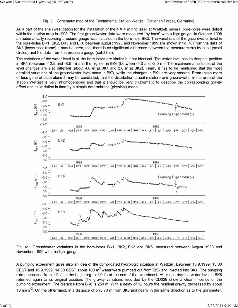
Fig. 3: Schematic map of the Fundamental Station Wettzell (Bavarian Forest, Germany).

As a part of the site investigation for the installation of the 4 × 4 m ring laser at Wettzell, several bore-holes were drilledwithin the station area in 1998. The first groundwater data were measured “by hand” with a light gauge. In October 1998an automatically recording pressure gauge was installed in the bore-hole BK3. The variations of the groundwater level inthe bore-holes BK1, BK2, BK3 and BK6 between August 1998 and November 1999 are shown in fig. 4. From the data ofBK3 (lowermost frame) it may be seen, that there is no significant difference between the measurements by hand (smallcircles) and the data from the pressure gauge (solid line).The variations of the water level in all the bore-holes are similar but not identical. The water level has its deepest positionin BK1 (between ‑12.5 and ‑8.5 m) and the highest in BK6 (between ‑5.0 and ‑2.0 m). The maximum amplitudes of thelevel changes are also different (about 4.0 m at BK1 and 2.0 m at BK2). Finally it has to be mentioned that the mostdetailed variations of the groundwater level occur in BK3, while the changes in BK1 are very smooth. From these moreor less general facts alone it may be concluded, that the distribution of soil moisture and groundwater in the area of thestation Wettzell is very inhomogeneous and that it should be very problematic to describe the corresponding gravityeffect and its variation in time by a simple deterministic (physical) model.

Fig. 4: Groundwater variations in the bore-holes BK1, BK2, BK3 and BK6, measured between August 1998 andNovember 1999 with the light gauge.

A pumping experiment gives also an idea of the complicated hydrologic situation at Wettzell. Between 15.9.1999, 13:00CEST and 16.9.1999, 14:00 CEST about 100 m3 water were pumped out from BK6 and injected into BK1. The pumpingrate decreased from 1.2 l/s in the beginning to 1.0 l/s at the end of the experiment. After one day the water level in BK6returned again to its original position. The gravity variations recorded by the CD029 show a clear influence of thepumping experiment. The distance from BK6 is 250 m. With a delay of 12 hours the residual gravity decreased by about10 nm s‑2. On the other hand, in a distance of only 70 m from BK6 and nearly in the same direction as to the gravimeter,


3 of 13 2/22/2011 9:40 AM

no clear changes of the water level occurred in BK3. If a groundwater regression coefficient rGW = 0.689 nm s‑2/cm isassumed (derived from the absolute measurements, see above) about 15 cm had to be expected. The downwarddirected bulge in the air pressure is not related to the pumping experiment.

A summary of all the precipitation, groundwater and soil moisture data available at Wettzell from the beginning of therecordings up to the end of January 2002 is given in fig. 6. The groundwater data measured with the light gauge (see fig.4) as well as the data from rain gauge RE2 were not included in the figure. The series of the rain data starts in April1998, the groundwater data followed in October of the same year (BK3, pressure gauge). The measurements of the soilmoisture started more than two years later in the end of December 2000.

Fig. 5: Pumping experiment. In the two frames at the right the vertical broken lines mark the time of the pumpingexperiment.

Within the precipitation data two small sections are marked by rectangles. In both cases gaps in the precipitation dataoccurred which are filled up with data from the nearby power station at the Hoellenstein reservoir (in a valley about 2 kmto the south-west from Wettzell, elevation difference about 200 m). Such manipulations are problematic from differentpoints of view, but better than data gaps. 4. Preparation of the SG-DataThe investigations concerned with the influence of groundwater variations on the gravity are based on the residualgravity, derived from the recordings of the superconducting gravimeter CD029 at Wettzell. “Residual gravity” means thatfrom the observed gravity data several “disturbing” influences are eliminated. It is of great importance, that the “right”influences are eliminated. In our case these are - Tides. In the period range greater than one month the amplitude factor 1.16 has to be used, regardless of the

results of the tidal analysis of local gravity data. Otherwise there is a risk, that the groundwater effect under study ispartly eliminated together with the tides.

- Air pressure. The influence of varying air density in the atmosphere is eliminated by a linear regression model, usingthe local air pressure variations at the gravimeter site and an regression coefficient derived by the standard tidalanalysis. More details of the air pressure model (e.g. regional air pressure distribution, deviations from the standardatmosphere) are not included.

- Polar motion. The gravity effect of polar motion has to be eliminated before any estimates of the instrumental driftare made. To this end IERS pole co-ordinates and the amplitude factor of 1.16 have to been used.

- Instrumental drift. Different constituents of the instrumental drift have to be taken into account. The exponential drift,occurring in the initial phase after the initialization of the gravimeter, has to be eliminated by fitting an exponentialmodel. After the exponential constituents have been eliminated, the remaining long-term drift in most cases may bedescribed by a linear model. If a sufficient number of absolute measurements is available, they may be used to


4 of 13 2/22/2011 9:40 AM

check the drift model derived alone from the data of the superconducting gravimeter. Commonly there is a goodagreement. In the case of discrepancies the residual gravity of the SG may be fitted linearly to the AG data and inthis way a corrected value of the drift rate may be found.

The data series of the CD029 is interrupted by a gap of about 6 weeks (May 5 – June 12, 1999), caused by total loss ofthe Helium. In the first section before the gap a strong linear drift of -136.15 nm s-2/month occurred in the lower system.After a careful re-initialization the drift-rate reduced to a very low value in the section after the gap. Altogether 9 absolutemeasurements were available, which could be used to correct the instrumental drift. The result is shown in theuppermost frame of figure 7. Especially in the second section of the data series a clear correlation between gravityvariations and changes of the groundwater level at BK3 can be recognized. Anomalies in the residual gravity can now beexplained simply by strong groundwater variations, e.g. the large peak of the residual gravity in the first half of 2000.

Fig. 6: Precipitation, groundwater and soil moisture at Wettzell from the beginning of the recordings up to the end ofJanuary 2002. The rectangles mark gaps in the precipitation data, which have been filled up with data from the nearbypower station at the Hoellenstein reservoir.

Unfortunately the first section of the data series recorded by the CD029 is supported only by two absolutemeasurements. Considering moreover the very strong linear drift and the remaining residuals of the exponentialconstituents, it may be concluded that the gravity data before the gap are very unreliable and therefore unsuited forfurther investigations.

5. Correlation between precipitation and gravityFrom equation (1) follows that in a closed hydrological system precipitation is the only input of water. The precipitationinfiltrates and distributes in the ground. In this way changes of the groundwater level and of the soil moisture arise.Inflow and run-off of water in the underground may change the situation in detail. However, precipitation measurementsin principle provide the most important input data of hydrological modeling.


5 of 13 2/22/2011 9:40 AM

Fig. 7: Corrections for the influences of precipitation and groundwater, applied to the residual gravity of the gravimeterCD029 at Wettzell.

The rain-meter used at Wettzell counts ticks of a rocker arm. However, there is always the problem to discern from thedistance between “no rain” and “no data due to a malfunction of the instrument”. In every case precipitation sensors mustbe maintained very carefully.Generally precipitation data may not be correlated directly with gravity changes. At first the precipitation (measured inheight or volume per unit of time) has to be converted into the corresponding gravity effect. For that purpose the simpleformula

(2)


6 of 13 2/22/2011 9:40 AM

was used, which was proposed and very successfully applied by D. CROSSLEY et al. [2] to correct a data seriesrecorded at Boulder. δgi is the contribution of the precipitation rj at the time j to the gravity change at the time i (i ≥ j). Toget the total time dependent gravity effect the single δgi have to be summed up over i and j. The time constants τ1 andτ2 stand for a multitude of different influences. According to the balance equation (1) τ1 describes the accumulation, i.e.the infiltration of the precipitation into the underground, and τ2 the consumption, i.e. the disappearance of the moisturedue to evapotranspiration and downward migration. Numerical values of τ1 and τ2 representative for a certain station arederived by fitting the mathematical model to the observed gravity data. In [2] the values τ1 = 4 hours and τ2 = 91 daysare given, which are valid for the local hydrological situation at Boulder. First attempts of hydrological modeling at Wett-

zell were done using the modified values τ1 = 4 hours and τ2 = 30 days [5,6 [1]].

Fig. 8: Precipitation and air temperature at Wettzell, 1.4.1998 – 30.6.2001. Modeled gravity effect of precipitationaccording to equation (2). First frame: precipitation. Second frame: air temperature. Three different values of the timeconstant τ2 were used in dependence of the air temperature. Third frame: long-term model (LTM). Fourth frame:short-term model (STM).

Many of the influences themselves vary during the year and as a consequence seasonal variations of the time constantsare to be expected too. A very expressive example are the variations of temperature which not only influence the directevaporation and the evapotranspiration (which additionally includes the contribution of the vegetation), but are alsoresponsible for the kind of precipitation (rain or snow) and for the state of the underground (frozen or not). Therefore theattempt was made to introduce time constants τ21, τ22 and τ23, being valid for the temperature ranges above 15°C,between 0 and 15°C, and below 0°C respectively. Examples of the gravity effect of precipitation modeled in this way aregiven in the third and the fourth frame of fig. 8. As may be seen from a comparison of both examples, the time constantsinfluence the amplitude of the modeled gravity effect. However, it has to be considered that no irreversible long-termaccumulation occurs. The greater values used in the long-term model (fig. 8, third frame), result in more pronouncedgravity anomalies as compared with the short-term model (fig. 8, fourth frame). Another example is given in fig. 12.There it could be shown, that the short-term model is equivalent to corrections derived from the directly measuredchanges of the groundwater level and variations of the soil moisture.


7 of 13 2/22/2011 9:40 AM

The relation between precipitation and gravity variations changes during the year. The correlogram is similarly muddledlike that of the groundwater influence (fig. 10, upper left frame), however it looks even less clear. At first for the relationbetween precipitation and groundwater as well as for the relation between precipitation and gravity changes regressioncoefficients were estimated over fortnightly periods. Similarly to the considerations with concern to the groundwaterinfluence (as described in the next paragraph) these fortnightly values were stacked with an annual period and averagedover the years (fig. 9). In a last step moving averages over every three neighboring values were derived. In this way thethick solid lines result, which more or less clearly show the seasonal variations of the regression behavior.

Due to the fact that precipitation cannot be directly correlated with changes of groundwater or gravity, the interpretationof the resulting regression coefficients differs slightly from that of the corresponding groundwater regression coefficients.With regard to the influence of precipitation on gravity the regression coefficients describe the deviations from therespective model and its parameters.

Fig. 9: Correlation between the modeled gravity effect of precipitation, groundwater and residual gravity. Stackedrepresentation of the regression coefficients. Horizontal bars: regression coefficients estimated over fortnightly periods inthe different years. Circles: mean values of the fortnightly regression coefficients over the years. Solid line: movingaverage of the fortnightly mean values. The vertical dotted lines separate the periods of high and low correlation.

As may be seen from the left frame of fig. 9 during the cold first months of the year as well as in the rainy autumn astrong correlation between precipitation and changes of the groundwater level occurs (upward curved sections of thesolid line), while in the remaining time of the year the influence nearly vanishes. The right frame shows, that the influenceof precipitation on the gravity has also a maximum in the cold season (snow cover, persistent frost), i.e. the modeledgravity effect during this time is too low. Due to increased run-off and evaporation the influence of precipitation is less inthe remaining time of the year. While in summer the observed values nearly correspond to the modeled effect(regression coefficient near 1.0), for two short periods in spring and in the early winter the influence is very low(regression coefficient near zero). 6. Correlation between groundwater and gravity

At the end of 2000 a first attempt was made to estimate the dependency of groundwater variations and gravity. Thisinvestigation was spread over the period 13.6.1999 – 31.12.2000. The result was the clear proof of a varying regressionbehavior during the year. From February to August groundwater variations have a strong influence on the gravity, whilefrom September to January the influence is weak.

At the end of 2001 a similar investigation was started on the basis of an enlarged data set. All data of the second part ofthe CD029 series having been available up to that time were included (i.e. all data after the large gap in May 1999). Atfirst sight the result was disappointing. The correlogram looks like a chaotic muddle of lines, obviously caused byresiduals of incompletely eliminated systematic influences (fig.10, upper left frame). However, if the correlogram isstudied more in detail (especially during the period when its visualization develops step by step on the screen of thecomputer), the visual impression alone suggests to distinguish between sections with weak slope and steeper ones. Aseparation of these sections results in the graphic representations shown in the upper right and the lower left frame offig. 10. The different slopes being characteristic for both subsets of the correlogram are clearly seen. However, like inthe total data set, the data of both subsets are not homogeneous. Therefore regression lines were separately derivedfor each uninterrupted section of the correlograms. The results are given in the lower right frame of fig. 10. The solid


8 of 13 2/22/2011 9:40 AM

lines relate to the weak sloped sections, the broken lines to the steep sections. The averaged regression coefficients are(0.248 ± 0.028) and (0.933 ± 0.048) nm s-2/cm respectively. These numbers very clearly confirm the visual impression ofdifferent slopes being characteristic for both subsets of the correlogram. If the fact of different slopes is neglected, theadjustment of the total data set (upper left frame) would result in a regression coefficient of (0.516 ± 0.003) nm s-2/cm.This value is near to the weighted mean of 0.476 nm s‑2/cm derived from the both seasonal values. The weights wereset proportional to the respective range of validity. The directly estimated total value as well as the weighted meancorrespond to the value of (0.689 ± 0.090) nm s-2/cm, derived from absolute measurements (fig. 1). However, due to theuse of only 9 separate absolute gravity values this first estimation of the groundwater regression coefficient is lessreliable than the later values on the basis of the continuous CD029 data series.

Fig.10: Correlation between groundwater and residual gravity. Seasonal variations of the groundwater regressioncoefficient

Generally correlograms have no relation to time. However, if the data are transferred to the time scale, the sections withdifferent regression behavior (described by the different regression coefficients) may be related to different times of theyear. From this kind of representation it becomes clear, that the periods with similar regression line slope repeat veryregularly from year to year. Therefore in a last step the data were stacked over a yearly period. The result is given infig.11, which very clearly shows the strong influence of groundwater changes from mid-May to mid-September (highregression coefficients, broken lines) and the weak influence from mid-September to mid-May (low regressioncoefficients, solid lines). The short sections of broken lines in February and November/December are related to themarginal sections of the data set and therefore may be ignored.


9 of 13 2/22/2011 9:40 AM

Fig. 11: Wettzell, 13.6.1999 – 31.12.2002. Stacked time intervals with similar regression behavior. The vertical dottedlines separate the period of strong groundwater influence (from mid-May to mid-September) from that of weakgroundwater influence (from mid-September to mid-May).

7. Examples of corrected gravity data

The change of soil moisture and groundwater after rainfall and the response of the gravimeter are clearly to berecognized, if short sections of the data series are studied. An example is given in fig. 12, covering the two monthlyperiod from October 1 to November 30, 2001. Between November 6 and 9 numerous rainfalls occurred (the plot isbased on the precipitation sums over 15 minutes each), which are followed by clear signals of the soil moisture as wellas the groundwater level. The vertical dotted line at November 7, 2001, 15:00 UT marks a steep rise of the soil moistureimmediately after the beginning of the rainfall. The groundwater level changes with a time delay of about two days. Afterthe rainfall both signals go down, the soil moisture more rapidly than the groundwater.The residual gravity (fifth frame from above) is also influenced by the rainfall. A clear peak is to be seen similar to thechange of the soil moisture. At last it has to be pointed out, that the modeled gravity effect of the precipitationcorresponds very well to the change of the residual gravity, especially to its amplitude. However, it decreases moreslowly than the residual gravity. - In the lowermost frame two attempts of corrections are shown.In the first variant the modeled gravity effect of precipitation is subtracted from the residual gravity (short-term model,second frame from above). However, for better approximation additionally a factor crain = 1.5 was used. Due to the fact,that the modeled gravity represents the total effect of precipitation, in this way changes of the soil moisture as well asthose of the groundwater level are corrected (assuming that the parameters of the model are chosen correctly). As maybe seen from the lowermost frame, the result of this correction is a clear diminution of the roughness of the curve.However, a total elimination of the precipitation influence could not be achieved.

In the second variant instead of the modeled gravity effect of precipitation the directly measured changes of soil moistureand of the groundwater level are used. The corrections are based on the groundwater regression coefficient 0.150 nms-2/cm, valid for the time between mid-September and mid-May, while for the soil moisture a value of 2.5 nm s-2/percentis assumed (roughly estimated from the graphical representations).If the results of both correction procedures are compared, no significant differences are to be recognized, i.e. bothvariants are equivalent. Strictly this is valid only for the example under consideration (1.10. – 30.11.2001, fig. 12). Fromother examples a similar visual impression results. However, details and the numerical values may differ.

The residual gravity during the total recording period of the CD029 at Wettzell is shown in fig. 13 (lowermost frame). Thetwo curves beneath are corrected for the influence of groundwater changes and additionally for the influence ofprecipitation (short-term model, instead of a soil moisture correction). As already mentioned, caused by certain reasonsthe first section of the record (before the gap in May, 1999) is unfavorably affected, and therefore it cannot be includedin the detailed studies. The second section is dominated by the large anomaly in the first half of 2000, clearly caused byan anomaly of the groundwater (uppermost frame). A similar behavior repeats in the first half of 2001. After thegroundwater correction was applied, the large anomaly in 2000 reduces considerably. Only a part of the second half ofthe anomaly remains. In contrast to that, the correspondent anomaly in 2001 seems to be overcompensated. As may beseen from the third curve below, the correction for precipitation has only a small influence. There are two exceptions. Atfirst the overcompensated groundwater anomaly in 2001 seems to be increased. The second exception concerns thesharp double anomaly in May 2000. While the second spike unambiguously is caused by a heavy rainfall, the first spikehas no correspondence to rainfall, soil moisture or groundwater. Therefore only the second spike vanishes after the datahave been corrected for the influence of precipitation. The first spike remains unchanged. To sum up it can be said that


10 of 13 2/22/2011 9:40 AM

the greatest part of the hydrological influences is eliminated by the groundwater correction on the basis of smootheddata, while details are covered by corrections for the influence of precipitation (modeled gravity effect of precipitation,STM). Residuals of the anomalies may remain or overcompensation may arise if the seasonal changes of the regressionbehavior are neglected.

Fig. 12: Hydrological influences at Wettzell, 1.10. – 30.11.2001. Groundwater values not smoothed. The vertical dottedline marks the date November 7, 2001, 15:00 UT. In the lowermost frame two different ways of hydrological correctionsare compared: firstly the modeled gravity effect of precipitation, secondly corrections derived from measured values ofthe groundwater level and of the soil moisture.


11 of 13 2/22/2011 9:40 AM

Fig. 13: Hydrological corrections, 1.4.1998 – 30.6.2001. Groundwater smoothed. The modeled gravity effect ofprecipitation (short-term model STM) is plotted in an enlarged scale (approx. 2:1) compared with the three curves in thelowermost frame. 8. Conclusions - The investigations presented here generally confirm, that gravity measurements may be affected significantly by

hydrological influences.

- At Wettzell an annual wave with a double amplitude of about 70 nm s-2 is to be expected, caused by variations of thegroundwater level throughout the year. The correction of such influences is of great importance for the investigationof other long-term phenomena (e.g. gravity effect of the polar motion).

- At Wettzell the long-term gravity effects are closely correlated with changes of the groundwater level, while themodeled gravity effect of precipitation better corresponds to the short-term gravity variations.

- At Wettzell the influence of groundwater variations may be described by a linear regression model with a meanregression coefficient in the order of 0.52 nm s-2/cm. However, between mid-May and mid-September the influenceseems to be stronger (0.93 nm s-2/cm) than in the remaining part of the year (0.25 nm s-2/cm).

- If the seasonal variations of the groundwater regression coefficient are neglected, errors may arise by over- orunder-compensation of the disturbing hydrological influences.

Acknowledgement

The authors express their thanks to


12 of 13 2/22/2011 9:40 AM

- the BKG, which permitted the use of the data and supported our investigations. - Thomas Klügel (FS Wettzell), who reliably made available the groundwater data and initiated the installation of the

soil moisture sensor. He always was ready for discussions and gave many hints with concern to the localhydrogeologic situation at Wettzell.

References

1. Harnisch, M., Harnisch, G.: Processing of the data from two superconducting gravimeters, recorded in 1990 - 1991 at Richmond (Miami,

Florida). Some problems and results. Marées Terrestres, Bull. Inf., Bruxelles (1995) 122, pp. 9141 - 9147

2. Crossley, D. J., S. Xu and T. van Dam (1998): Comprehensive Analysis of 2 years of SG Data from Table Mountain, Colorado. Proc. 13th Int. Symp. Earth Tides, Brussels, July 1997. Obs. Royal Belgique, Brussels 1998, 659 – 668.3. Harnisch, M., Harnisch, G.: Hydrological Influences in the Registrations of Superconducting Gravimeters and Ways to their Elimination. Marées Terrestres, Bull. Inf., Bruxelles 131 (1999), pp. 10161 - 10170

4. Harnisch, M., Harnisch, G., Nowak, I., Richter, B., Wolf, P.: The Dual Sphere Superconducting Gravimeter C029 at Frankfurt a.M. and Wettzell. First Results and Calibration. Cahiers du Centre Européen de Géodynamique et de Séismologie, Luxembourg 17(2000), pp. 39 - 56

5. Harnisch, M., Harnisch, G., Jurczyk, H., Wilmes, H.: 889 Days of Registrations with the Superconducting Gravimeter SG103 at Wettzell (Germany). Cahiers du Centre Européen de Géodynamique et de Séismologie, Luxembourg 17(2000), pp. 25 - 38

6. Harnisch, M., Harnisch, G., Nowak, I., Richter, B., Wolf, P.: The Dual Sphere Superconducting Gravimeter GWR CD029 at Frankfurt a.M. and Wettzell. First Results and

Calibration. IAG Symposia, Vol. 121, Springer-Verlag Berlin Heidelberg 2000, pp. 155 - 160

7. Falk, R.: Deutsches Schwerereferenzsystem (DSRS). Deutsches Schweregrundnetz (DSGN) Poster. INTERGEO, Berlin 2000

[1] In [6] the false value τ2 = 91 days is given instead of the right value 30 days


13 of 13 2/22/2011 9:40 AM

Documents

Seasonal Variations of Hydrological Influences · Seasonal Variations of Hydrological Influences ... their state of weathering and tectonic influences (formation of clefts and cavities