6

Table 2. Correlation of skid numbers with texture data.

Tire Coefficient Data

Test Type ao a1 a2 R2

Fall 1978 SNB -19.68 0.64 0.41 0.813 SNR -7.83 0.80 -0.12 0.740

Spring 1979 SNB -16.87 0.54 0.50 0.906 SNR -9.19 0.74 0.15 0.926

ferent sign for the two data sets. The coefficients a1 and a2 for the blank tire are similar in magnitude, which indicates comparable sensitivity to microtexture and macrotexture.

CONCLUSIONS AND RECOMMENDATIONS

The results of this study indicate that the ribbed E501 test tire provides a good evaluation of micro­texture but is not sensitive to macrotexture, which is felt to be a significant factor in wet-pavement safety. This may account for a lack of correlation between skid~resistance measurements by using the ribbed tire and accident statistics.

Ideally, a pavement skid-resistance survey would be performed by using both the ribbed E501 and the blank E524 tires. By comparing the skid-resistance values from both tires, one can readily estimate the levels of microtexture and macrotexture and assess the cause of poor skid resistance and likelihood of success of corrective action.

In the event that skid-resistance surveys can be performed with one tire only, the blank E524 tire appears to be the stronger candidate. At this writing, no attempts to correlate smooth-tire data with accident frequency are known to me, although in one state some data are reportedly being collected. A study to relate blank-tire data to accident fre­quency should be conducted to verify this conclusion.

Since this research was initiated, the manu-

Transportation Research Record 788

facture of the E524 tire has been suspended due to lack of demand. Preliminary tests indicate that a used E501 tire that has the ribs machined away com­pletely and has been subjected to a 350-km (200-mile) break-in produces results that are in ex­cellent agreement with those of the E524 tire. Such a tire will not have a long useful life but will serve as an interim tire for research until demand for the blank tire increases.

REFERENCES

1. R. J. Rasmussen. Pavement Surface Texturing and Restoration for Highway Safety. Presented at the 53rd Annual Meeting, HRB, 1974.

2. v. R. Shah and J. J. Henry. Relationship of Locked-Wheel Friction to That of Other Test Modes. Pennsylvania Department of Transporta­tion, Harrisburg, Final Rept. on Agreement 52489, Feb. 1977.

3. R. L. Rizenbergs, J. L. Burchett, J. A. Deacon, and C. T. Napier. Accidents on Rural Interstate and Parkway Roads and Their Relation to Pavement Friction. TRB, Transportation Research Record 584, 1975, pp. 22-36.

4. R. ~. Rizenbergs, J. L. Burchett, and L. Warren. Accidents on Rural, Two-Lane Roads and Th'eir Re­lation to Pavement Friction. Kentucky Bureau of Highways, Frankfort, Research Rept. 458, 1976.

5. J. J. Henry. The Relationship Between Texture and Pavement Friction. Presented as 1977 Kummer Lecture at ASTM Annual Meeting, St. Louis, MO, Dec. 1977.

6. D. C. Mahone. An Evaluation of the Effects of Tread Depth, Pavement Texture, and Water Film Thickness on Skid Number--Speed Gradients. Virginia Highway and Transportation Research Council: Federal Highway Administration, U.S. De­partment of Transportation, March 1975.

7. Interim Recommendations for the Construction of Skid-Resistant Concrete Pavement. American Con­crete Paving Association, Oak Brook, IL, Tech. Bull. 6, 1969.

Seasonal Variations in the Skid Resistance of Pavements in Kentucky

JAMES L. BURCHETI AND ROLANDS L. RIZENBERGS

Frequent measurements of skid resistance were made on 20 pavements in common use in Kentucky from November 1969 through 1973. Principal analysis involved relating changes in skid resistance to day of the year and re· lating skid resistance to temperature at the time of test, to average antecedent temperatures, and to average rainfall. Seasonal variations exhibited an annual sinusoidal cycle. The changes in sand-asphalt and bituminous concrete surfaces under high volumes of traffic were about 12 skid numbers (SNsi. The changes in portland cement concrete (PCCI and bituminous concrete under low volumes of traffic were about 5 SNs. The lowest SN values occurred in early to mid· August for PCC and sand-asphalt pavements and in late August to early Septem· ber for bituminous concrete. Correlations between changes in SN and tem­perature were best for ambient air temperature averaged over four- and eight­week periods prior to date of test. However, correlations between changes in SN and temperature were not so good as correlations between SN and day of the year. On the other hand, combining traffic volumes in the form of de­viations from yearly average daily traffic with temperature yielded correlations with SN that were as good as correlations between SN and the day of the year. It was concluded that skid=resistancc measurements in Kentucky should

be conducted between the first of July and the middle of November to assure detection of significant differences in SN. However, frequent testing of refer­ence sections is recommended to define more specifically each year the be­ginning and ending dates of the testing season.

Laboratory studies of wear and frictional characteristics of aggregates in Kentucky began in 1956, and field testing of pavement surfaces began in 1958. Many variables associated with testing devices, procedures, and methods of test were investigated and led eventually to standardization. From 1958 to 1969, field tests were conducted with an automobile in several modes (!l. Testing then was confined mostly to a six-month period from mid-May through mid-November. Also, the greater

Transportation Research Record 788

manpower needs for testing with an automobile could best be satisfied in the summer. However, concerns persisted with regard to the influence of weather and the seasonal changes. A limited investigation of seasonal changes was conducted during 1965, 1966, and 1967. Results then indicated significant fluctuations, but the data were insufficient to define the change (2).

A two-wheeled skid-test trailer was acquired in 1969 and was adapted for routine testing <1>· Statewide surveys were initiated, and the data were used for a multiplicity of purposes, which included the identification of hazardous locations in wet weather. The test period needed to be defined to minimize variability. Also, measurements outside the test period needed to be adjusted to a common base.

Periodic measurements were initiated in 1969 on 20 pavement sections; there were four types of surfaces. Tests were conducted from November 1969 through 1973. Changes in skid res i stance were related to day of the year. Relationships were sought between skid resistance and temperature at the time of test, average temperature for one to eight weeks prior to the day of test, and average rainfall. This paper presents those analyses.

DATA

Pavement Sections

A total of 20 pavement sections was selected that were within 48 km (30 miles) of Lexington. Fourteen were 2.4 km (1.5 miles) long and the other six were 1.6 km (1.0 mile) long. The sections were bituminous (class 1, types A and B), sand-asphalt, and portland cement concrete (PCC). The annual average daily traffic (AADT) per lane ranged from 200 to 10 300. Each section was at leas t three years old; therefore, polishing effects due to traffic had stabilized.

Weather

Precipitation and temperatures were obtained from monthly Environmental Data Service tabulations of local climatological data for the Lexington area. Average precipitation was determined in terms of both quantity and duration. Average temperatures for periods of one, two, three, four, and eight weeks preceding tests were calculated from daily average temperatures, which were determined by averaging 3-h readings. Monthly average tempera­tures were recorded. Ambient air temperature and pavement surface temperature were measured and re­corded at the time of test.

Skid-Resistance Measurement

Skid resistance was measured with a surface-dynamics pavement friction tester (model 965A) manufactured by K. J. Law Engineers, Incorporated, Detroit , Michigan. The two-wheeled skid-test trailer was acquired in 1969. This trailer complied with ASTM E274-70. The measurements represent the traction developed between a standard 36-mm (14-in) test tire (AS'llol. E249-66) and a wetted pavement. The locked-wheel measurements are expressed in skid numbers (SNs) •

From November 1969 to December 1972, the test sections were tested on a monthly basis. Six of the sections were overlaid in June 1972. Testing continued during March and June 1973 on the 14 remaining sections. Equipment malfunctions, weather conditions, and other circumstances prevented testing during some months. In all, tests were made

7

during two-thirds of the scheduled months. Measurements were made in the left wheel path at

17.9 m/s (40 miles/h). Tests were also made at 8.9 m/s (20 miles/h) and at 26.8 m/s (60 miles/h) during one-half of the schedule.

SN VERSUS DAY OF YEAR

From the 17. 9-m/s tests, the SN was plotted versus date of test. These plots indicated that the SN varies sinusoidally during the year. It was desirable to derive an equation to indicate the day of occurrence of the highest and lowest SN values. Therefore, the model equation for the regression analysis was based on the cosine function; one cycle encompassed 365 days. This equation was as follows1

SNP = SN8 -C.SN cos (360°(0- Da)/365]

where

= predicted SN, SN about which SN varies, largest variation of SN about SNa, day of year, and day of year at which SN is lowest.

(I)

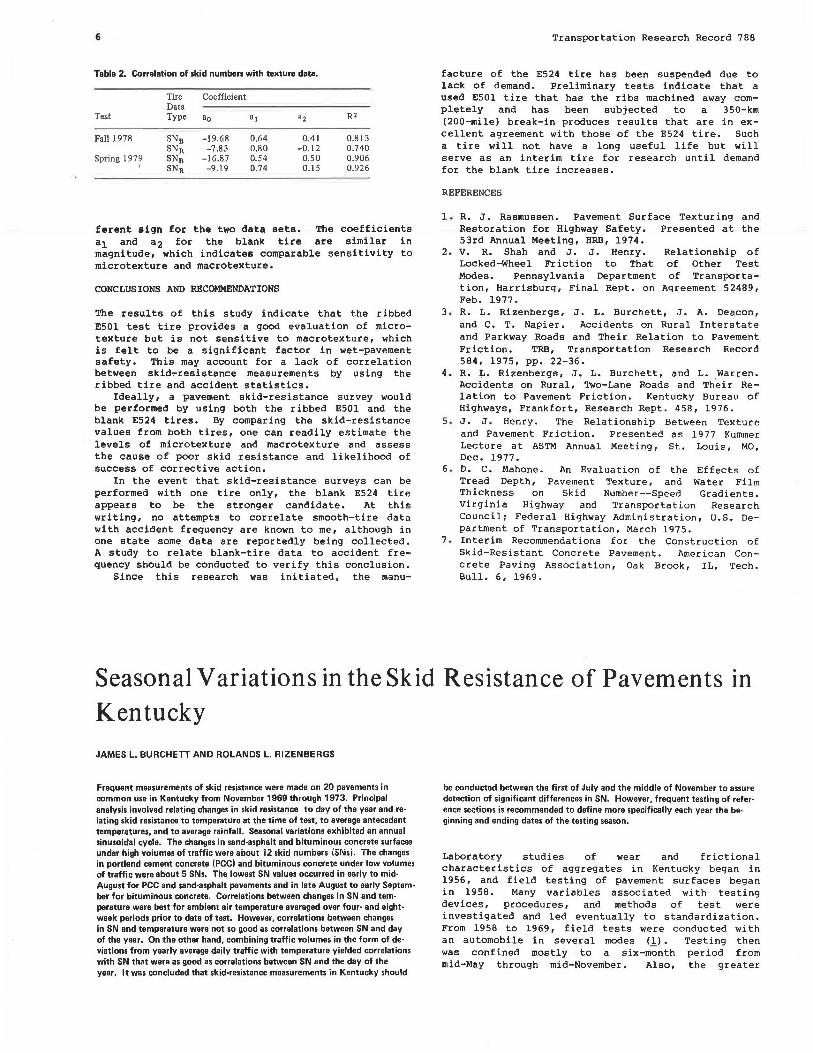
The values of SNa, 6SN, and D1 were determined for each test section by using the method of least squares. These values, along with other statistics, are presented in Table 1. The variations in SN were d etermined for each sec t ion by subtracting SNa f rom SNP. The resulting curves are s hown in Figure 1.

The variances in SN on bituminous surfaces were associated with traffic volume. For example, section 1, which has a 16-point change, was the same construction project as section 2, which had only a 12-point change. Section 1, however, was the outer lane and had a higher AADT than did section 2. The same was true for pairs of sections 5 and 6, 7 and 8, 9 and 10, and 17 and 18. All other sections were on two-lane roads and therefore pairs of sections had nearly the same AADT. These pairs were sections 3 and 4, 11 and 12, and 19 and 20. There was very little difference in the SNs in those cases.

Changes in · the SN (SN - SNal for each type of surface were combined, and regression equations were determined. Class 1, type A and B bituminous

Table 1. Results of regression analysis for SN versus day of year, by pavement section.

Section SN8 C.SN Di Dtt Rl E,

I 43.5 8.0 248 65 0 .735 3.6 2 52.7 5.8 252 69 0.587 3.6 3 37 .0 7.0 248 66 0 .39 1 6.7 4 36.8 6.6 253 70 0.492 5.1 5 53 .7 2.4 226 44 0 .234 3.6 6 65 .0 1.6 222 39 0.156 2.9 7 41.8 5.1 225 43 0.588 2.9 8 5 1.6 3.5 248 65 0.463 2.7 9 49.0 8.1 246 63 0.670 4.2

10 60.2 4 .0 260 78 0.335 4.0 II 49.6 2.7 238 55 0 .191 4.2 12 48.9 3.0 256 73 0.177 5.0 13 36.6 3.9 231 49 0.282 4.5 14 43.4 4.7 206 24 0.318 5.1 15 42 . l 2.2 315 132 0.223 3.0 16 46 .3 2.3 190 7 0.175 3.5 17 38.0 6.8 231 49 0.640 3.8 18 40 .5 5.9 215 33 0.509 4.3 19 45 .2 3.8 207 25 0.408 3.5 20 43 .8 5. 1 207 25 0.720 2.4

Note: Dh • day of year at which SN is highest (Oh= DJ -182.5) ; R2 =coefficient of correlation; E5 =standard error of the estimate .

8

Figure 1. Best·fit curves for SN variation versus day of year for each test section, by pavement type.

a: w

"' lE :::> z

0 ;;;:

"'

0

-5

•IO

s

Transportation Research Record 788

SAND - ASPHALT SURFACE

PORTLAND CEMENT CONCRETE SURFACE

SEC'rlON NUMBER

'" Cl • ) <I a: w > CLASS I, TYPE B, BITUMINOUS SURFACE <I

10

~ a: ~ .... >-

lE 0 0

TEST SECTION a: ... -5

"' z 0 j:: ~ -10 > w 0

CLASS I, TYPE A, BITUMINOUS SURFACE

30 60 90 120 150 180 210 240 270 300 30 360 DAY OF YEAR

JAN I FEB I MAR I APR I MAY I JUN I JUL I AUG

MONTH OF YEAR SEP I OCT I NOV I DEC I

Table 2. Results of regression analysis for deviations from yearly average SN versus day of year.

Pavement Type SN8 llSN D1 Dh R2 E,

Class I, type A -0. l 5.3 248 65 0.402 4.8 AADT > 3500 0.0 6.8 250 68 0.508 5.0 AADT < 3500 0.0 2.0 225 42 0.198 3.2

Class l , type B 0.1 4.1 243 61 0.346 4.1 AADT > 3500 -0.1 5.6 239 56 0.536 3.6 AADT < 3500 0.1 3.1 251 68 0.215 4.3,

PCC 0.0 2.5 223 40 0.150 4.2 Sand-asphalt 0.0 5.4 218 36 0.537 3.7

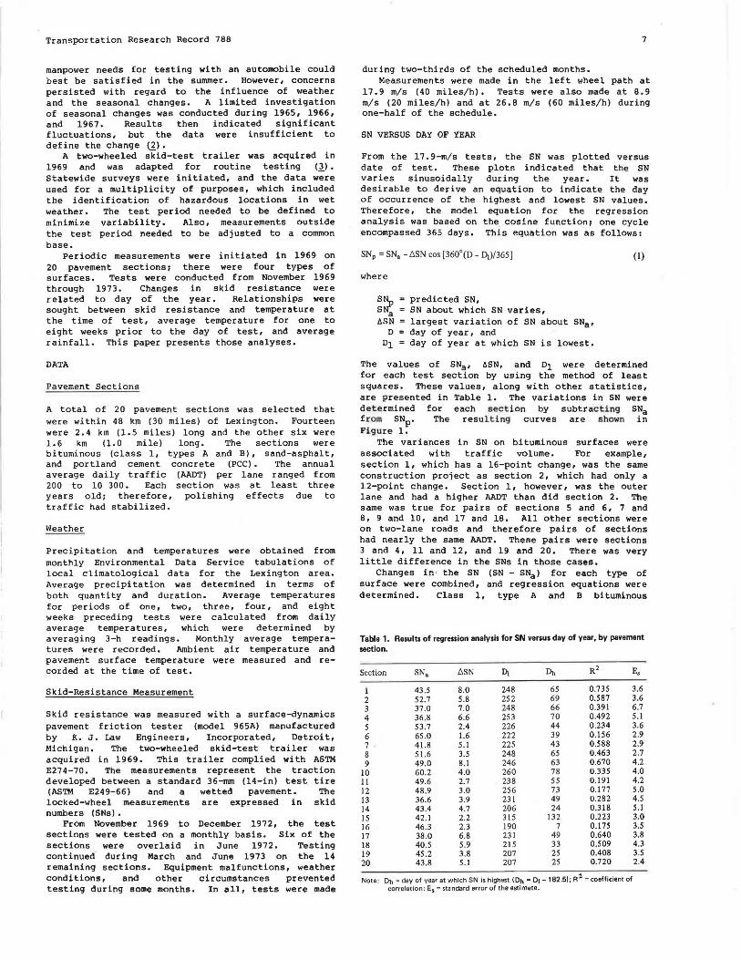
pavements were also divided into two groups: AADT greater than or less than 3500 vehicles per day per lane. The equations and their coefficients are given in Table 2. Regression curves for the 365-day cycle are given in Figure 2. Data and curves are in Figures 3-5.

The regression curves indicated that SNs for class 1, type A that had the higher AADT varied seasonally by 14 points; the lowest SN occurred in early September. The SN for class 1, type A that

had the lower AADT varied by 4 points, and the lowest SN value occurred in mid-August . The SN fQr class 1, t ype B surfaces t ha t had the higher AADT varied seasonally by 11 points, and those with the lower AADT varied by 6. The lowest SN values for those pavements occurred in late August and early September, respectively. The SN fnr Pr.r. p;ivP.mentio; varied seasonally by 5 po ints. The lowest value occurred during mid-August. The SN for sand­asphalts varied seasonally by 11 points (lowest in early August) .

PRECIPITATION AND TEMPERATURE VERSUS DAY OF YEAR

The mechanisms that change pavement surface character is tics are many and have been enumerated elsewhere (i l. Two factors investigated in this study and that may be associated witjl these mechanisms were precipitation and temperature.

Since changes in the SN correlated with day of the year, factors associated with the principal mechanisms that cause variances must also correlate with day of the year. Figure 6 is a plot of monthly averages of precipitation and temperature. The amount and duration of precipitation and air

Transportation Research Record 788

Figure 2. Best-fit curves for SN variation versus day of year for test sections grouped by pavement type.

Figure 3. SN variation versus date of test for class 1, type A bituminous pavement, grouped by AADT.

SAND - ASPHALT SURFACE

0

a: ~ PORTLAND CEMENT CONCRETE SURFACE

; _:.__f ___ ~----Al.-L -SE-CTIO-NS ___ a ___ ____, ~ a:

~ 10 .--~~~~~~~-C_L_A_s_s~_r_,~_T_Y_P_E~_B_,~~B_IT_U_M~IN_o_u_s~~s_u_R_~_A_C_E~~~~~~~~-.

0 ~ AADT < 3, 500

~ ( SECTIONS 10, II, ANO 12 )

(/) z 0

-5

3,500 (SECTIONS 7, 8, AND 9)

SECTIONS

~-10 ~~~~~~~~~~~~~~~~~~~~~~~~~~~~~~~~~~~~~

> w 0

0 AADT < 3,500

I SECTIONS 5 AND 6 )

- ~

-100 30 60 90

JAN FEB I MAR I APR

20

a: w 10

"' ::; :::> z 0

0 ~ · 10

"' w -20

"' <( a: w > <(

~ 20 a: <( w 10 >-

::; 0 \:: 0

a: LL

·10 (/) z 0 t= -20 :'! _J <C > z "' ~ _J <C

> ;;i ~ 0

" <(

;;i w w z " " "' 0 I 1969 I 1970

120

> 3,500 I SECTIONS I, 2, 3, AND 4 )

SECTIONS

150 180 210 2•0 270 300 330 360 DAY OF YEAR

MAY I JUN I JUL I AUG SEP I OCT I NOV I DEC I MONTH OF YEAR

AADT < 3,500

AADT > 3,500

I I

> z "' ,.

~ <C > z "' ~ _J <C i5 z "' ~ 0

" <( <(

~ 0

" <(

;;i ~ " <(

z " " z " " z " " I 1971 I 1972 I 1973

9

_J

;;i

JUL

lo SEP en <O

NOV

JAN

MAR

(0 MAY

(3 JUL

SEP

NOV

JAN

MAR

MAY <O :~ JUL

SEP

NOV

- JAN

MAR

-- MAY <0 -~ h:I JUL

SEP

NOV

'"7-JAN

-- MAR <O -~ CJol MAY

JUL

PRECIPITATION (WATER) (INCHES)

o gggg g PRECIPITATION

( WAITR) (MILLIMETERS)

PRECFITATION DURATION (HOURS, 01 11 (0.25 mm) OR MORE)

1:)~~~~g~~

e ::!! ~ ... CD C .... ~ 0 CD ~ O> CD•

!!: > :r c 3 ~ 0 .. ~ 'i :::r"§I 0 CD ""'n M -6' e ... ~~­i g S· ! a. a. . -CD

3 ... .. ill

AMBIENT AIR TEMPERATURE ( • F)

N OI 6 Cl' 00 00

, 1 I

1'

~ a g:

I l

II

II

111

1 1

II I I

II I

I

J I I

'1 I I

1. ' ' ' ' Ji, 0-Ul()(j~ :x

AMBIENT AIR TEMPERATURE (°C)

Ill .,, ::iG' is .... -g. !" !- ~ ii c c .. .. ~ 3 iii' CD =t. :I 0 !f :I c ..

;: 5 ! .. s. ;: ~

~ ~ n n .. :I a.

DEVIATIONS FROM YEARLY AVERAGE, SKID NUMBER

~ t o o ~ ~ a o a ~ JUL

~ SEF'

"' NOV

- JAN

MAR

_ MAY

"' (3 JUL

SEP

NOV

-JAN

MAR

MAY co ::! JUL

SEP

NOV

JAN

MAR

- MA'

"' jj JUL

SEP

NOV

JAN

...- MAR

"' -.I l.lol MAY

JUL

~=

(1l

"~ Or z,. "z 21 0

"' -to ...... "" "' z -t

I•

.. ..

~ ,. i ,. !::;

•

~::!! I--'

i'I! 0

mil

i:"" e en 3 z f: c: ~.

i g. c :I

~ 3 ~~ ~! c .. is. .{ i ~~ on. ~ .. . a .-

DEVIATIONS FROM YEARLY AVERAGE, SKID NUMBER ' ~ 0 0 ~

~ ~ 0 5 2l 0 0 0 - JUL

~ SEP

"' NOV

JAN

MAR

MAY iii ~ JUL

SEP

NOV

- JAN

MAR

MAY iii ::::! JUL

SEP >cl ... Ill

NOV ::i DI

JAN '8 ... MAR rT

"' rT _ MAY

"' j:j JUL

SEP

,. .... 0 ,. ::i 0 ,.

I I t :. -t ,. A

:.i 0 f1) -t "' DI

"' f1) NOV

JAN

0 Ill .!"

I I \' 0 ...

"' 0 0 "' 0

_MAR

"' ~MAY

:.i f1) 0 0 ...

JUL Q.

.., "" ""

Transportation Research Record 788

temperature correlated somewhat with month of the year.

Precipi tation

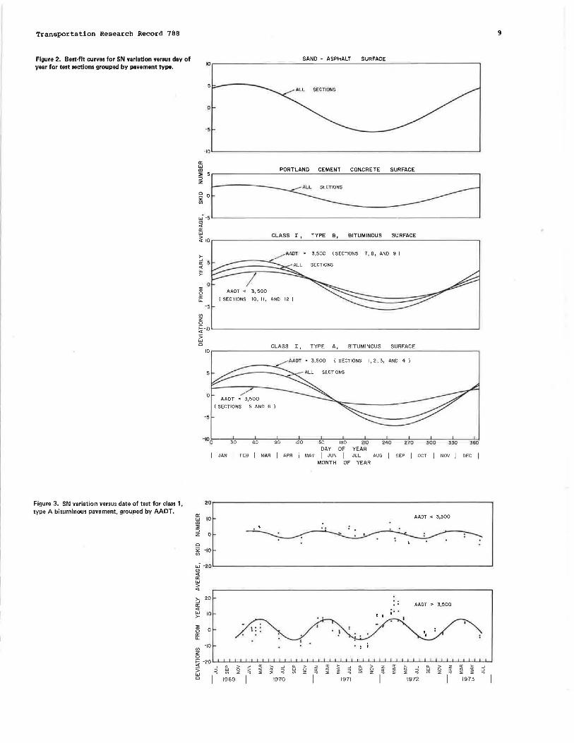
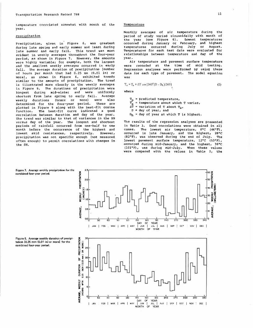
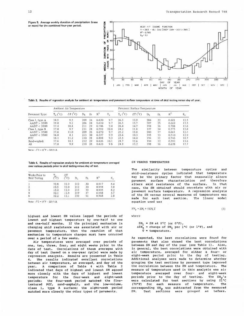
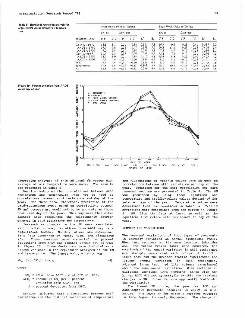
Precipitation, given in Figure 6, was greatest during late spring and early summer and least during late summer and early fall. This trend was most evident in weekly averages throughout the four-year period, as shown in Figure 7. However, the amounts were highly variablei for example, both the largest and the smallest weekly averages occurred in early fall. The average duration of precipitation [number of hours per month that had 0.25 mm (0.01 in) or more], as shown in Figure 6, exhibited trends similar to the amounts of precipitation. The trend is illustrated more clearly in the weekly averages in Figure 8. The durations of precipitation were longest during mid-winter and were uniformly shortest from late spring to early fall. Average weekly durations (trace or more) were also determined for the four-year period. These are plotted in Figure 9 along with the best-fit cosine function. The best-fit curve indicated a good correlation between duration and day of the year. The trend was similar to that of variances in the SN versus day of the year. The longest and shortest periods of rainfall occurred from one-half to one month before the occurrence of the highest and lowest skid resistances, respectively. However, precipitation was not specific enough (not measured often enough) to permit correlations with changes in the SN.

11

Temperature

Monthly averages of air temperature during the period of study varied sinusoidally with month of the year (see Figure 6). Lowest temperatures occurred during January or February, and highest temperatures occurred during July or August. Temperatures for each test date were evaluated for relationships between temperature and day of the year.

Air temperature and pavement surface temperature were recorded at the time of skid testing. Regression analyses were performed by using these data for each type of pavement. The model equation was

Tp =Ta+ L'.T cos [360°(0 - Dh)/365) (2)

where

Tp predicted temperature, Ta temperature about which T varies, t.T variation of T about Tar

D day of year, and Dh day of year at which T is highest.

The results of the regression analyses are presented in Table 3. Good correlations were obtained in all cases. The lowest air temperature, 8°C (46°F), occurred in late January, and the highest, 28°C (82°F), was observed during the end of July. The lowest pavement surface temperature, 12°C (53°F), occurred during mid-January, and the highest, 38°C (101°F), was during mid-July. When these values were compared with the values in Table 2, the

Figure 7. Average weekly precipitation for the combined four-year period.

2.5,...-- ---------------- -----------------,

Figure 8. Average weekly duration of precipi­tation [0.25 mm (0.01 in) or morel for the combined four-year period.

I 0~5 "' " 10:

0~0!:---~3~0;:---~6~0-----,9~0,...--~12~0--..,,15~0---...,1~so;:---~21~0---,,2i40,,_-2~1~0-~,o~o--3~3-o--3~s~o' 0 ~

DAY OF YEAR JAN I FEB I MAR I APR I MAY I JUN JUL I AUG SEP I OCT I NOV I DEC

MONTH OF YEAR

W W ~ ~ I~ ~ W - 270 30 0 330 360 DAY OF YEAR

JAN I FEB I MAR I APR I MAY I JUN I JUL I AUG SEP I OCT I NOV I DEC I MONTH OF YEAR

12

Figure 9. Average weekly duration of precipitation (trace or morel for the combined four·year period.

Transportation Research Record 788

BEST ·FIT COSINE FUNCTION Y • 26.5 - 16.1 COS [ 360° I DAY • 207 i I 365 ) R' • 0,785 E5 "' 6.l

00!-~~30,......~~i;o.,.._~-90~~---'12Lo~~15~0~~,~so~~-2~10~~2~4-o~-2-1~0~~3~oo~~:n~-0~~3s,_..o

DAY OF YEAR JAN I FEB I MAR I APR I MAY I JUN I JUL I AUG SEP I OCT I NOV I DEC I

MUNTN OF YEAR

Table 3. Results of regression analysis for ambient air temperature and pavement surface temperature at time of skid testing versus day of year.

Ambient Air Temperature Pavement Surtace ·femperature

Pavement Type T8 (°C) 6T(° C) Dh Di R2 E, Ta (°C)

Class I, type A 18.5 9.5 209 26 0.630 9.7 26 .S AADT > 3500 19.0 9 .2 206 24 0.610 9.7 26.S AADT < 3500 17.4 10.4 211 29 0.706 9.4 26.4

Class 1 , type B 17'.0 9.7 211 28 0.593 10.4 24.2 AADT > 3500 17.8 11.0 209 26 0.670 9.7 25.2 AADT< 3500 16.8 8.1 213 30 0.537 9.9 23.6

PCC 18.I 11.2 210 28 0.698 9.3 23 .5 Sand~asphalt 17.6 JO.I 212 29 0.636 JO.I 24.7 All 17.8 9.9 210 28 0.633 9.8 24.9

Note: t°C= (t°F -32)/1.8.

Table 4. Results of regression analysis for ambient air temperature averaged over various periods prior to skid testing versus day of test.

Weeks Prior to T 6T Skid Testing ld'C) (°C) Dh Di R2 E,

I 12.8 12.3 212 30 0.917 4.8 2 12.5 12.0 212 30 0.944 3.8 3 12.2 12.3 215 33 0.935 4.2 4 12. l 12.4 219 37 0.958 3.7 8 12.2 12.l 233 51 0.968 2.8

Note: t°C = (t°F -32)/1.8.

highest and lowest SN values lagged the periods of lowest and highest temperature by one-half to one and one-half months. If the principal mechanism in changing skid resistance was associated with air or pavement temperature, then the reaction of that mechanism to temperature changes must have occurred over a period of a few weeks.

Air temperatures were averaged over periods of one, two, three, four, and eight weeks prior to the date of test. Correlations of these averages with day of test (based on a one-year cycle) were made by regression analysis. Results are presented in Table 4. The results indicated excellent correlations between air temperature, as averaged, and day of the year. A comparison of Table 4 with Table 2 indicated that days of highest and lowest SN agreed more closely with the days of highest and lowest temperature for the four-week and eight-week periods: the four-week period matched the fine­textured PCC, sand-asphalt, and the low-volume, class 1, type A surfacei the eight-week period matched more closely the other types cf pavements ~

6T(°C) Dh Di R2 E,

13.9 204 22 0 .681 12.5 13.7 207 25 0.669 12.5 14.7 198 16 0 .708 12.6 11.8 197 14 0 .575 12.8 13.8 200 17 0.661 12.4 10.3 195 13 0.510 12.9 14.8 194 II 0.746 10.7 12.6 194 12 0.592 13.6 13 .2 198 16 0.638 12.7

SN VERSUS TEMPERATURE

The similarity between temperature cycles and skid-resistance cycles indicated that temperature may be the primary factor that seasonally alters pavement surface characteristics and therefore alters skid resistance of the surface. In that case, the SN obtained should correlate with air or pavement surface temperature. A regression analysis of the SN versus several measures of temperature was made for each test section. The linear model equation used was

where

SN at 0°C (or 0°F), change of SNi per 1°C (or 1°F), and temperature.

(3)

As expected, the best correlations were found for pavements that also showed the best correlations between SN and day of the year (see Table 1). Also, in general, the best correlations were obtained with air temperature, averaged for either a four- or eigh t -week period p r ior to the day of test i ng. Additional analyses were made to determine whether grouping the test sections by pavement type improved the correlation between the SN and temperature. The measure of temperature used in this analysis was air temperature averaged over four- and eight-week periods prior to the day of testing. The SNp's were calculated for test sections by using 21°C (70°F) for each measure of temperature. The corresponding SNp was subtrac,ted from the measured SN . Test s ect i ons were g r,m p<>il "'" hefore.

Transportation Research Record 788 13

Table 5. Results of regression analysis for Four Weeks Prior to Testing Eight Weeks Prior to Testing adjusted SN versus ambient air tempera·

ture.

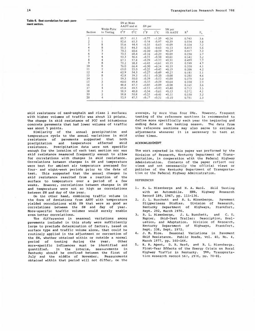
Figure 10. Percent deviation from AADT versus day of year.

SNi at

Pavement Type 0°F 0°C

Class I, type A 14.8 8.1 AADT > 3500 17.9 9.6 AADT< 3500 7.0 3.8

Class I, type B 11.4 6.3 AADT > 3500 14.7 8.0 AADT < 3500 7.9 4.4

PCC 7.9 4.4 Sand-asphalt 17.8 9.8 All 12.8 7.0

!.! ~o ... ... "' a: I- o - INTERSTATE

o • PARKWAY

~ 20 • - FOUR LANES DIVIDED

i'ISNi per

]oF 1°c R2

-0.21 -0.38 0.307 -0.26 -0.47 0.358 -0.10 -0.18 0.250 -0.16 -0.29 0.268 -0.21 -0.38 0.417 -0.11 -0.20 0.154 -0.11 -0.20 0.151 -0.25 -0.45 0.588 -0.18 -0.32 0.296

SNi at i'ISNi per

E, 0°F 0°C ]oF !°C R2 E,

5.3 16.4 9.4 -0.23 -0.41 0.337 5.2 5.7 20.3 11.5 -0.29 -0.52 0.424 5.4 3.1 7.4 4.7 -0.10 -0.18 0.234 3.1 4.5 12.l 7.1 -0.17 -0.31 0.274 4.5 4.1 15.4 8.8 -0.22 -0.40 0.403 4.2 4.5 8.6 5.2 -0.12 -0.22 0.171 4.4 4.4 8.0 4.6 -0.12 -0.22 0.143 4.6 3.6 18.0 IO.I -0.26 -0.47 0.532 3.8 4.7 13.6 8.0 -0.19 -0.34 0.294 4.8

a c " - FOUR LANES UNDIVIDED • - TWO LANES

... -" "' 10 a: ... ~

~ 0 a:

"' ... >-~ 0 - 10 a: ... z 0

!;i ·20 5 ... c

I-~ - 300 w w m ~ ~ ~ w ~ 270 300 330 360 a: DAY OF YEAR ... 0.. JAN I FEB I MAR I APR I MAY I JUN JUL I AUG SEP I OCT I NOV I DEC I

Regression analyses of this adjusted SN versus each average of air temperature were made. The results are presented in Table s.

Results indicated that correlations between skid resistance and temperature were not so good as correlations between skid resistance and day of the year. For these data, therefore, prediction of the skid-resistance cycle based on correlations between SN and temperature would not be so accurate as those that used day of the year. This may mean that other factors have confounded the relationship between changes in skid resistance and temperature.

Inasmuch as changes in the SN were associated with traffic volume, deviations from AADT may be a significant factor. Monthly volume was determined from data presented by Agent, Herd, and Rizenbergs <.~). These averages were converted to percent deviations from AADT and plotted versus day of year in Figure 10. These deviations were included as a second variable in the regression analyses of the SN and temperature. The linear model equation was

where

SNi SN at mean AADT and at 0°C (or 0°F), 6SNa change in SNi per 1 percent

deviation from AADT, and A percent deviation from AADT.

(4)

Results indicated that correlations between skid resistance and the combined variables of temperature

MONTH OF YEAR

and fluctuations of traffic volume were as good as correlations between skid resistance and day of the year. Equations for the best correlation for each pavement section are presented in Table 6. The SN was predicted by using these equations and temperature and traffic-volume values determined for selected days of the year. Temperature values were determined from the equations in Table 5. Traffic deviations were determined from the curves in Figure B. SI\> fits the data at least as well as the equations that relate skid resistance to day of the year.

SUMMARY AND CONCLUSIONS

The seasonal variations of four types of pavements in Kentucky exhibited an annual sinusoidal cycle. When test sections at the same location (shoulder and lane versus median lane) were compared, the magnitude of the annual variation in skid resistance was strongly associated with volume of traffic. Lanes that had the greater traffic experienced the largest annual variation in skid resistance. Adjacent lanes that had like volumes experienced about the same annual variation. When sections at different locations were compared, those with the higher AADT did not necessarily exhibit the greatest changes in SN. Other factors apparently confounded the correlation.

The lowest SN during the year for PCC and sand-asphalt pavements occurred in early to mid­August. The lower SN for class 1 surfaces occurred in late August to early September. The change in

14 Transportation Research Record 788

Table 6. Be1t correlation for each pave· ment section. SN at Mean

AADTand at SN per Weeks Prior

Section to Testing 0°F

I I 85.7 2 I 82.6 3 8 55.6 4 8 55.5 5 3 70.2 6 3 73.5 7 4 53.3 8 4 67.] 9 8 73.2

10 8 76.0 II 2 63.0 12 4 62.9 13 8 42.8 14 I 59.3 15 3 60.0 16 3 48.8 17 4 65.8 18 3 58 .9 19 2 58.8 20 4 52.9

skid resistanc e o f sand-as phal t and class 1 surfaces with higher volumes of traffic was about 12 points. The change in skid resistance of PCC and bituminous concrete pavements that had lower volumes of traffic was about 5 points.

Similarity of the annual precipitation and temperature cycle to the annual variations in skid resistance of pavements suggested that both precipitation and temperature affected skid resistance. Precipitation data were not specific enough for the location of each test section nor was skid resistance measured frequently enough to allow for correlations with changes in skid resistance. Correlations between changes in SN and temperature were best for ambient air temperature averaged for four- and eight-week periods prior to the date of test. This suggested that the annual changes in skid resistance resulted from a reaction of the surface to temperature over a period of a few weeks. However, correlations between changes in SN and temperature were not so high as correlations between SN and day of the year.

On the other hand, combining traffic volume in the form of deviations from AADT with temperature yielded correlations with SN that were as good as correlations between the SN and day of year. More-specific traffic volumes would surely enable even better correlations.

The differences in seasonal variations among pavements included in this study were sufficiently large to preclude determination of factors, based on surface type and traffic volume alone, that could be routinely applied in the adjustment or correction of the SN, whether obtained within or outside a normal period of testing during the year. Other more-specific influences must be identified and quantified. In the interim, measurements in Kentucky should be confined between the first of July and the middle of November. Measurements obtained within that period will not differ, on the

0°C JoF l°C SN per 1% AADT R2 E,

6 l.l -0.77 -1.39 +0.54 0.743 3.6 65.3 -0.54 -0.97 +0.39 0.554 3.8 44.4 -0.35 -0.63 +0.09 0.324 7 .2 44.3 -0.35 -0.63 +0.13 0.413 5.6 60.6 -0.30 -0.54 +0.24 0.417 3.2 68.4 -0.16 -0.29 +0.09 0.230 2.9 46.6 -0.21 -0.38 +0.01 0.542 3.2 57.8 -0.29 -0.52 +0 .31 0.499 2.7 58.8 -0.45 -0.81 +0.15 0.599 4.7 66.4 -0.30 -0.54 +0.19 0.350 4.1 55.0 -0.25 -0.45 +0.19 0.208 4.2 54.3 -0.27 -0.49 +0.27 0.181 5 .I 39.3 -0. 11 -0.20 -0.08 0.285 4.6 50.0 -0.29 -0.52 +0.09 0.379 5.0 49.4 -0.33 -0.59 +0.64 0.330 2.9 47.2 -0.05 -0.09 -0.08 0.165 3.6 49.5 -0.51 -0.92 +0.40 0.713 3.5 48.0 -0.34 -0.61 +0.13 0.572 4.1 50.8 -0.25 -0.45 +0. 11 0.530 3.2 47.5 -0.17 -0.31 -0.10 0.751 2.3

average, by more than four SNs. However, fr equent testing of the reference sections is recommended to define more specifically each year the beginning and ending date of the testing season. The data from the reference sections may also serve to estimate adjustments whenever it is necessary to test at other times.

ACKNOWLEDGMENT

The work reported in this paper was performed by the Division of Research, Kentucky Department of Trans­portation, in cooperation with the Federal Highway Administration. Contents of the paper reflect our v iews and not necessarily the official views or policies of the Kentucky Department of Transporta­tion or the Federal Highway Administration.

REFERENCES

1. R. L. Rizenbergs and H. A. Ward. Skid Testing with an Automobile. HRB, Highway Research Record 189, 1967, pp. 115-136.

2. J. L. Burchett and R. L. Rizenbergs. Pavement Slipperiness Studies. Division of Research, Kentucky Department of Highways, Frankfort, Rept. 292, March 1970.

3. R. L. Rizenbergs, J. L. Burchett, and C. T. Napier. Skid-Test Trailer: Description, Eval­uation, and Adaptation. Division of Research, Kentucky Department of Highways, Frankfort, Rept. 338, Sept. 1972.

4. J. M. Rice. Seasonal Variations in Pavement Skid Resistance. Public Roads, Vol. 40, No. 4, March 1977, pp. 160-166.

5 . K. R. Agent, D. R. Herd, and R. L. Rizenbergs. First-Year Effects of the Energy Crisis on Rural Highway Traffic in Kentucky. TRB, Transporta­tion Research Record 5b 7 , 1976, pp. 70-81.