Seasonal patterns of futures hedging and the resolution of output uncertainty

JOURNAL OF ECONOMIC THEORY 53, 304327 ( 1991)

Seasonal Patterns of Futures Hedging and the Resolution of Output Uncertainty*

DAVID HIRSHLEIFER

Anderson Graduate School of Management, University of Califorrlia at Los Angeles,

Los Angeles. California 90024

Received May 9, 1989; revised July 2, 1990

Optimal futures hedging is examined in a two-good model with stochastic output and sequential information arrival. A producer’s optimal hedge depends on demand elasticity, sensitivity of his output to weather. his correlation with aggregate output, and how rapidly his output uncertainty is resolved relative to other producers during different seasonal periods. Because regional output uncertainties are resolved at different times, the optimal futures position of a grower will commonly reverse in direction during the crop year. A producer with non-stochastic output who faces price risk arising from demand shocks may remain unhedged or even maintain a long position, Journa/ qf Economic Liferature Classification Numbers: 022. 521. 714. :(’ 1991 Academic Press. Inc.

An issue that is central to the analysis of commodity futures markets is the determination of optimal hedging positions of producers. To the extent that growers or handlers of a commodity are risk-averse, they have an incentive to hedge on the associated futures market to offset the revenue variability of their businesses. If other means of risk reduction such as equity issuance are costly, owing either to transaction costs or to the problems of moral hazard and adverse selection, futures hedging becomes an important means of controlling risk.

Most research on optimal hedging has employed models that are “partial equilibrium,” in the sense that the consumption choice between the commodity underlying the futures contract and other commodities is not modeled. Instead, decisionmakers are assumed to derive utility from generalized wealth, which is equivalent to assuming only a single consump-

* I thank a referee of this journal, Avi Kamara, Warren Bailey and Francis LongstaR for helpful comments.

304 0022-053 l/91 $3.00 Copyright CI 1991 by Academic Press. Inc. All rights of reproduction in any form reserved

SEASONAL PATTERNS OF FUTURES HEDGING 305

tion good.’ Since the payoff on a futures contract is determined by the stochastic price of the underlying commodity relative to other goods, it is more satisfactory to model futures trading in a setting in which individuals consume distinct goods. The current paper examines optimal patterns of hedging through time within a general equilibrium (multi-good) setting.

A number of general equilibrium papers on futures have examined different issues. [ 13, 10, 27,4] provide a number of useful results concerning hedging by producers in two date models. [2, 121 allow for multiple trading rounds, but focus more on futures pricing than on the factors deter- mining optimal hedging decisions. [3] examined the ability of traders to achieve efficient allocations using instantaneously expiring futures contracts in continuous time; it did not focus on seasonal patterns of hedging.

This paper provides a multigood model in which information arrives sequentially, and resolves uncertainty at different rates for different growers depending on the time of year. An obvious consequence of sequential information arrival is that hedgers are given an opportunity to rebalance their futures positions repeatedly.

As will be seen, the need to rebalance is intensified by the fact that for most crops uncertainty about output is resolved at different times for different growers. For example, with respect to the orange juice futures market, uncertainty about whether a freeze will harm the Florida orange crop is resolved at a different time of year from the resolution of the Brazil crop. News about own output, versus news about others’ outputs, has very different effects on a grower’s revenue distribution, as well as upon the payoff of his futures position. These two types of information therefore lead to different hedging incentives. We will see that the hedging position implied by anticipated news about the outputs of other growers is likely to be of opposite sign to the position needed to hedge against news about own output. This may lead to drastic rebalancing of optimal hedging positions as the rates at which different types of information arrive vary through the year.

The paper is structured as follows. The economic setting is described in Section 1. Section 2 analyzes dynamic hedging strategies when uncertainty arises either within or outside the commodity market. Section 3 concludes the paper. All proofs are contained in the Appendix.

1. THE ECONOMIC SETTING

Before trading, each individual begins with an endowment of a stochasti- tally variable quantity of a risky commodity 2 and a non-stochastic quan-

I These papers include [24, 21 chapter 13, 111 in single period settings, and [I, 291 in a multiperiod setting.

306 DAVID HIRSHLEIFER

tity of the numeraire commodity N (“all other goods”).’ In the assumed trading regime of Futures Markets (FM), individuals can exchange only riskless claims to Z and N. Thus, the purchase of a claim to Z entitles the buyer to future delivery of one unit in each and every state of the world. The market regime excludes the possibility of trading claims that are state-contingent, e.g., insurance contracts or equity shares. Spot and futures markets are assumed to be competitive, and individuals are assumed to have homogeneous (agreed) beliefs and rational expectations.

Consumption takes place at a single date after all information has arrived and all trading has been completed. Individuals maximize expected utility by trading to alter their consumption levels of goods N (the numeraire) and Z (corn). Preferences may differ across individuals, but are assumed to be additively separable: U(n, r) = u(n) + v(z).~ If growers do not desire the good that they produce, they have o(z) = 0. Let there be S possible states of the world after all information has arrived. Information is publicly revealed through a sequence of m information events with binary outcomes, which are jointly conclusive.4 (I.e., the realization of the entire sequence determines a single state of the world, so that S = 2”‘.)

Each information event i is a random variable dJ whose possible outcomes are denoted & and bj. The history of information events through j is (0’, 9*, . . . . tY) and will be denoted by sj. The entire ordered sequence of information events 1 through m determines the final state srn (or more briefly, s). The initial probabilities are rrz for the different states, and after later events 8l, . . . . 8’, the probability of state s conditional on history s’ is denoted rti.

The sequence of trading under FM is as follows. Each participant begins with an endownment position E = (5; Z,, . . . . Z,), where ti is his initial (non- random) endowment of N available for consumption at the terminal date, and 5, (s= 1, . . . . S) is his state-distribution of Z. (Superscripts for the individual are suppressed except where needed for clarity.) As polar cases, we can think of a “typical consumer” endowed only with N (2, = 0), and

‘We may interpret Z as corn, say, and N as all non-corn consumption. The purpose of assuming a fixed endowment of N is to focus on risk due to variability in the size of the crop. We allow for variability in N instead of in Z in Section 2.3. A stock market could be introduced (see, e.g., [28, 111) if, in addition to a futures contract on Z, equity shares were traded on stochastic endowments of N.

3 Introducing riskless consumption at a date just prior to the first trade would not substantively alter any of the results provided here. On the other hand, allowing for additional future-dated consumption and resttlement would introduce other considerations which are not addressed in this paper.

4 The binomial information process is used for tractability, as discussed further below. [6] used a binomial state process to provide insight about hedging behavior in options. In contrast with its model, which assumes an.exogenous process for prices, this paper derives prices as part of a market equilibrium.


of a “typical grower” endowed with some state-distributed pattern of Z (his prospective output of corn, say), and possibly some N as well. Before the first information event, each individual trades on the futures market to a new position To = (no; zy, . . . . z” S). This initial futures transaction involves a purchase (possibly negative) of claims to to units of future corn at price PO (in units of N). (Thus, for a buyer, zy exceeds 5, by 5’ for each and every s.) After the first information event 0’, each individual revises his belief to rcr and retrades (by buying or selling 5’ contracts at price P’) to a new trading position T’. This process of information arrival and retrading continues until 0” arrives and resolves the final state of the world. Each individual then trades at the ultimate (spot) price P” to his final consumption positions (n”; z’: ). (Note here that after the semicolon only z; appears, the quantity of Z in state S, which is the single state actually realized.)

The individual’s trading problem may then be written as

{$a$) ECW”) + WY1 subject to

,o = 6 - po40, $ = ,,,k - 1 - pkrk

z;=&+(O, Z;=z;-‘+<k, k = 1, . . . . m s = 1, . ..) s.

The trading strategies t” are functions of sk, the history through k. The selection of the tk’s, by the trading constraints, determines Z: and nk as functions of sk, a dependence which is left implicit. Prices Pk are also functions of history. I” takes on value zr in state S. Although the private and social endowments of N are riskless, 6” is also in general random, since it arises from a trading strategy that depends on stochastic information arrivals.’

Effective Completeness of the Futures Markets Regime. On the basis of the mild assumption that different event realizations lead to different prices (otherwise, perturb the endowments to shift prices slightly), an essential lemma is obtained.

LEMMA 1. The regime of Futures Markets is effectively complete.

To see why intuitively,6 let us define WY as wealth contingent on state s for an individual after all information has been revealed (when 0” arrives) but prior to the final round of trading. Let contingent wealth be the value

5 For the special case u = 0, it is also necessary to impose the non-negativity constraint z: > 0, which will be binding because otherwise the individual could always increase his utility by selling more Z in the final round to buy more N.

6 A more rigorous proof appears in [ 121.


of his total holdings n”-’ and z;~’ of N and Z in state s, denominated in units of N:

(2)

A trader’s “wealth” at all earlier rounds is defined formally in the Appendix. In general, if there are enough securities to adjust the level of “wealth” achieved due to different outcomes at each information event, then the market is effectively complete. A futures contract just suffices here because of the binomial information structure.’ The assumed information structure therefore allows us to exploit the tractable properties of complete markets allocations, while capturing the need for traders to use futures contracts.8

2. EQUILIBRIUM FUTURES PRICES AND OPTIMAL HEDGING

Section 2.1 summarizes without proof a result concerning the pricing of futures contracts.’ Then, in the heart of the paper, Section 2.2 analyzes optimal hedging by diverse producers, and Section 2.3 examines hedging when producers face shocks on the demand side.

2.1. Futures Price Bias

Proposition 1 asserts that the futures price is an unbiased predictor of any later futures price, including the final spot price.” This “martingale” result is far from being a universal truth about futures pricing; rather, it arises from three stylized features of the current model: additively separable preferences, I1 effectively camp lete markets, and non-random endowment of the numeraire. Let EJ be the expectation conditional on history si.

‘It is by now well established that multiple rounds of trading can reduce the number of long-lived securities needed to complete a market. See, e.g., [18]; [7] provide a continuous time analysis. The binary information structure is the discrete time analog to a diffusion framework with a single state variable. In the current model, absent transaction costs, an efficient allocation is achieved using only the futures contract for the exchange of N and Z.

a Unlike options pricing models, here there are no redundant securities. With more than two possible information outcomes at each event, more securities would be required to complete the market. This would introduce portfolio holding considerations which will not be our focus here.

9 [ 121 provides a fuller treatment of this result and how it is moditied when there are fixed setup costs of trading.

i” Similar martingale results, with non-random quantity of the numeraire commodity, have been provided by [ 131 in a two-state model, and [23] in a continuous time setting. [25] stressed the sensitivity of this result to complementarity between goods.

” The result is consistent with the limiting case in which growers have u(z) = 0.

SEASONAL PATTERNSOF FUTURESHEDGING 309

PROPOSITION 1. Under a regime of Futures Markets, prices folfow a martingale, that is, Pj= E’[Pk] for all k >j.

A number of partial equilibrium models have predicted that the futures price will be an upward or downward biased predictor of the later spot price according to whether aggregate hedging by producers is long or short. In the current model, so long as the endowment of N is non- stochastic, the futures price is unbiased regardless of whether producers hedge long or short. This difference occurs because the analysis explicitly allows for consumption of commodities rather than generalized wealth. The intuition is that producers and consumers have complementary risk positions, and hence consumers are willing to take futures positions opposite to producers without demanding a premium. Consider a group of pure consumers endowed only with N. In the case of inelastic demand, producers will tend to hedge short, because their price risk is large relative to their quantity risk. (See the discussion following Proposition 2 below.) The partial equilibrium theory maintains that an outsider requires a downward bias (i.e., positive risk premium) in the futures contract to compensate for the risk of taking a long futures position. However, this neglects the state-dependence in consumers’ indirect utility of wealth function.”

Consumers begin with a non-stochastic endowment of N, so without futures trading, their wealths are independent of state. Nevertheless, since the final spot price at which they can purchase Z is random, they do bear consumption risk. With inelastic demand, a consumer spends more on corn when the price is high than when it is low, so a high price reduces his consumption of N. Owing to additive separability, this implies high marginal utility of the numeraire. Thus, a long position is a good hedge for a consumer, because the futures contract pays off more when his marginal utility of wealth is higher. (A short position is a good hedge in the case of elastic demand.) Thus consumers and producers are mutuall-v hedging by taking the opposite futures positions.13

2.2. Seasonal Patterns of Futures Hedging

To illustrate the general thrust of the analysis, for concreteness I use the additive logarithmic (LOG) family of utility functions

I2 A consumer’s marginal indirect utility is a function not only of his (N-denominated) wealth, but of the price of corn (Z).

I3 The supply and demand for futures contracts is equated at a risk premium of exactly zero because in an effectively complete market with non-stochastic aggregate N and addititively separable preferences, individuals optimally arrange their consumptions of N to be level across states. Thus, even though wealth is not equated across states, the marginal utility of wealth ( = u’(n)) is. Therefore, at their optimal positions individuals are not on the margin willing to pay a premium for a security to shift contingent wealths across states.

642!53/2-7


U(n, z) = M log(n) + log(z - p), (3)

where CI and /? are constants, c1> 0. a measures the relative intensity of preference for N versus Z. CI may vary across individuals, implying differen- ces in their desire for corn (Z).14

Let yld refer to elasticity of consumption demand for Z with respect to the round-m spot price for Z. It follows (see Appendix) that in a market in which growers and consumers have LOG preferences (possible with different preference parameters c(), or in which consumers have LOG preferences and growers have LOG-N preferences, the demand for corn is elastic or inelastic according to /?, i.e.,

lyldl)<l as PSO. (4)

For use in describing optimal hedging positions, let the correlated relative sensitivity of two variables, CRS, be defmed as

EC Yl CRS(X, Y) = b,, - = dW/ECJ-1 cov(X, Y)

ECU Pxy c( Y)/E[ Y]’ where b,,-

r?(Y) ’

(5)

and pxr is the correlation between X and Y (the equality containing pxr applying only if a(X) # 0). The CRS is also the regression coefficient of the percentage deviations from the mean on X on Y. Let the total number of individuals in the population be K, let lowercase 5 refer to an individual producer’s endowed quantity, and 2 to per capita output, i.e., the market- wide aggregate quantity divided by K. The CRS reflects two factors which, as we will see in Proposition 2, help determine optimal positions: (1) the correlation of information about the producer’s output with news about aggregate output (pz in the single event case), and (2) the relative sensitivity of his adjusted output to environmental influences (as measured by the ratio of coefficients of variation, (a(.?)/(E[?] - fi))/(c(Z)/(E[Z] - p))). Let CRS’ refer to the value based on a distribution conditional on history sj. Let Hj= xi=, tk be the total futures position of an individual at time j, and let the “hedge ratio” be Hj/(Ej[FJ - /?), the ratio of the total futures position to adjusted expected output. The main result of the paper is:

PROPOSITION 2. If consumers and producers have LOG preferences, then:

I4 Under more general preferences, growers might want to assort across locations according to their risk tolerances, which would in general affect the relationship between hedging positions and output distributions. However, in the current setting the market is effectively complete, which eliminates the incentive to match locations with preferences.


(1) The optimal hedge at time j of individual i, H”, is

,,=Ei+‘C(z-B)/(Z-P)l-E~+‘C(z-P)/(Z-P)] E~+‘[l/(Z-B)]-E~+‘[l/(Z-B)] . (6)

(2) If there is a single conclusive anticipated information arrival (m = 1) and EC;] # /I,

Hi E[E] - p

=CRS(z-/I, z-p)- 1. (7)

(3) With many information arrivals, if E’[?] # B,

H”

E’[?] -p = CRS’(Ei+ ‘[r] - fl, Ej+ 1 [z] _ B) _ I

+ O(d) + O(aS) + O(a$z). (8)

where O(X) indicates a quantity that approaches zero at the same rate as X.”

Proposition 2 provides formulae for predicting seasonal variations in optimal hedging positions that can be empirically implemented by using data on regional outputs, the spot price, the number of growers, and total population size. l6 The correlation and relative sensitivities (CRS’) of revisions in the expected outputs of different regions can be estimated using seasonal crop forecasts that are available from the United States Department of Agriculture and a number of private services.

I5 In order for the utility function (3) to be defined, society’s output of Z must exceed sub- sistence, i.e., .??, > r7 in all states. It is likely that I?‘[?] > fl for a grower, i.e., he is producing more corn than he needs for his own consumption. Note 18 gives formulae that apply even if E’[Yj =/I

r6 The preference coefficient 8, which is a measure of demand elasticity, can be estimated from output and spot price data. By (16)

or summing over the K individuals,

Hence, the intercept coefficient in the regression of aggregate output on the reciprocal of the spot price, when divided by the population size K gives 8.


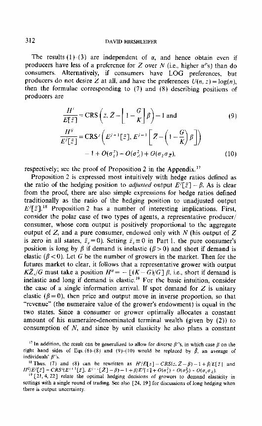
The results (1 k(3) are independent of a, and hence obtain even if producers have less of a preference for Z over N (i.e., higher ~4’s) than do consumers. Alternatively, if consumers have LOG preferences, but producers do not desire Z at all, and have the preferences U(n, z) = log(n), then the formulae corresponding to (7) and (8) describing positions of producers are

~=,,,(,,,-[l-~]p)-land

[z-(I-$])

(9)

- 1 + O(d) + o(o;) + O(a,az), (10)

respectively; see the proof of Proposition 2 in the Appendix.17 Proposition 2 is expressed most intuitively with hedge ratios defined as

the ratio of the hedging position to adjusted output E’[Z] - fi. As is clear from the proof, there are also simple expressions for hedge ratios defined traditionally as the ratio of the hedging position to unadjusted output E’[Z].‘” Proposition 2 has a number of interesting implications. First, consider the polar case of two types of agents, a representative producer/ consumer, whose corn output is positively proportional to the aggregate output of Z, and a pure consumer, endowed only with N (his output of Z is zero in all states, 5, = 0). Setting 5, = 0 in Part 1, the pure consumer’s position is long by B if demand is inelastic (/I > 0) and short if demand is elastic (/3 < 0). Let G be the number of growers in the market. Then for the futures market to clear, it follows that a representative grower with output KZ,/G must take a position H” = - [(K - G)/G] 8, i.e., short if demand is inelastic and long if demand is elastic.” For the basic intuition, consider the case of a single information arrival. If spot demand for Z is unitary elastic (/I = 0), then price and output move in inverse proportion, so that “revenue” (the numeraire value of the grower’s endowment) is equal in the two states. Since a consumer or grower optimally allocates a constant amount of his numeraire-denominated terminal wealth (given by (2)) to consumption of N, and since by unit elasticity he also plans a constant

” In addition the result can be generalized to allow for diverse /Y’s, in which case p on the right hand sides of Eqs. (6t(8) and (9t( 10) would be replaced by 1, an average of individuals’ fi”s.

i* Thus (7) and (8) can be rewritten as H’/E[?] = CRS(5, Z-p)- 1 +/~/E[z] and H’/IE’[?]‘= CRS’(E’+‘[z], E’+‘[Z] -/I- 1 +p/E’[?] + 0(a:)+ O(u$) + O(a,crz).

I9 c 21 4 221 relate the optimal hedging decisions of growers to demand elasticity in , , settings with a single round of trading. See also [24, 191 for discussions of long hedging when there is output uncertainty.


expenditure on Z, he will hedge to achieve constant wealth across states. The value of a pure consumer’s endowment position is non-random, and that of a grower also leads to constant revenue, so each selects a neutral futures position. This is consistent with (7) with b = 0; for a typical grower z - is proportional to Z, so that CRS = 1, leading to a zero hedge.

With inelastic demand, price risk dominates quantity risk, and is hedged with a short position since this risk is positively correlated with the futures contract payoff. That is, with inelastic demand individuals want to expend more of their terminal wealth on Z when price is high. Since a consumer will allocate a constant amount to consumption of N, he must raise his wealth in high price states by holding a long futures position. A grower, on the other hand, finds that the value of his Z endowment is higher in the low output state, labelled h, than in the high output state, a, because low output ?b is more than offset by a disproportionately high spot price. Since he plans to consume more N than his endowment level, the difference in his revenues across states is larger than the variations in his planned expenditures on Z. He is thus motivated to sell futures (short hedging) in order to divest part of his (predominantly price) risk. The sale of a 1 : 1 bundle of claims to Z in either state reduces the value of the grower’s Z holdings more in state b than in state a. So selling futures short has the effect of raising state-u wealth and reducing state-h wealth, which stabilizes the grower’s wealth values. With elastic demand, on the other hand, quantity risk dominates, and is hedged with a long positions (since quantity is negatively correlated with price). In other words, revenue is higher in state b instead of a, so the grower is motivated to go long in futures.20

In contrast to the case of perfectly correlated growers, Proposition 2 shows that the position of a grower whose output is unrelated to aggregate output or unaffected by the information event, so that CRS = 0, by Part 2 is Hi = -E[5] + /I. Hence, such a grower takes a partial hedge of his expected output if fl> 0, and hedges more than fully if b < 0.21

Since the “typical” grower (whose output of Z is proportional to the ‘aggregate economy-wide total) hedges short under inelastic demand and

” TO see that this intuitive argument is consistent with (7), consider what happens to CRS for a representative producer as p is increased from 0, leading to inelastic demand, Since 5 = (K/G) Z, where K > G. an increase in fi reduces E[Z] - b by a greater percentage than E[i] -/r. It follows from the definition of CRS in (5) that CRS(z- fi, Z - fi) > 1, so that the hedge ratio CRS - 1 is negative. Similarly, p < 0, elastic demand, implies that CRS < 1. so that a producer’s optimal hedge is positive. A similar argument holds for (9); since G/K< 1, as p increases from zero, Z - [ 1 - (G/K)] p decreases, while t is unchanged.

” The grower adjusts the full short hedge long with inelastic demand or short with elastic demand for the same reason that pure consumers take long or short positions: to finance his personal planned consumption expenditure on Z. Thus, if growers do not care about Z, by (9) a grower whose output is independent of the aggregate simply sells short his expected output.


long under elastic demand, to further interpret Proposition 2 it is useful to examine the case of unit elastic demand (p=O, by (4)). Under unit elastic demand, identical producers would take null futures positions, so this case gives a useful baseline for appraising the effect of disparate output distributions on the optimal hedge. I will refer to this case as simple LOG preferences. I begin with the case of a single conclusive information event.22 An example then follows that illlustrates the seasonal variations in hedging brought about by multiple information arrivals.

Single Information Arrival. A producer with high CRS has a good fair- weather farm; when aggregate output is high, his output is disproportionately so, compared to other growers.23 A grower buys (sells) futures as CRS > ( < ) 1, so that a grower with CRS = 1 will not trade futures. In fact, under simple LOG preferences, consumers also stand patz4

We saw above that since output and spot price vary inversely, price and quantity risks offset. With simple LOG preferences, implying unit-elastic demand for corn, the offset is perfect, so that the wealth values of the endowment of a typical grower are equal in the two states. The CRS incor- porates two factors: sensitivity to and correlation with the aggregate. Two farms might both be highly sensative to rain versus shine, although one is subsject to drought, the other to flooding. If aggregate output is higher when there is rain (state a), then the former correlates with the aggregate, and the latter against.

It is useful to view these cases in terms of contingent wealths. The first grower is endowed with higher wealth when state a occurs, and lower wealth in state b. To reduce risk, he will purchase futures. This raises his state-b wealth and reduces his state-a wealth, since the spot price P’ is higher in the low-output state. The reverse holds for the second grower. The conclusion is that producers with good poor-weather farms sell futures, and those with good fair-weather farms buy futures.25

The intuitive arguments concerning the effects of demand elasticity,

*’ A related result with a single information arrival was derived by 1211 in a mean-variance model; see also [20, 241.

ZA typical grower has CRS = 1, and a weighted average across growers of their CRS”s equals 1, where the weights are output shares, wi= E[,?‘]/KE[Z].

24 1261 has applied this idea in an attempt to explain the introduction of organized futures trading for some commodities in the U.S. during 186G1880. It uses a statistic based on the CRS parameter derived in Proposition 2 to measure the diversity of output distributions for different geographical regions. This variable proved to be a predictor of the existence of futures trading.

” A producer endowed with a non-random output has a good poor-weather farm, because in the low output state his output is comparatively high. His CRS is zero, so he will “fully hedge” by going short to the extent of his entire output, to equalize contingent wealths across the two states.


correlation with aggregate output, and relative sensitivity on the optimal hedge are fairly robust with respect to alternative assumptions about preferences. These parameters will in general determine how growers’ revenues are related to their planned expenditures on 2. So long as individuals wish to consume non-stochastic quantities of N, futures trading will be used to align the numeraire-denominated wealths with their planned expenditures across states of nature.‘6

Multiple Information Arrivals. With many information arrivals, the optimal hedging strategies will vary in predictable seasonal patterns for growers expecting news about output to arrive at different times. The following example shows that the dynamic strategy differs dramatically from what would be predicted by a single-event model.

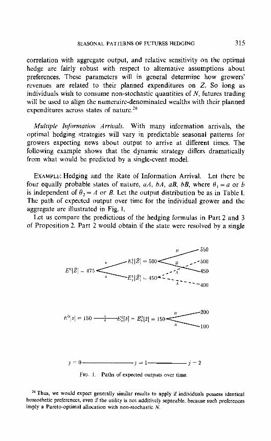
EXAMPLE: Hedging and the Rate of Information Arrival. Let there be four equally probable states of nature, aA, bA, aB, bB, where O1 = a or b is independent of 6, = A or B. Let the output distribution be as in Table I. The path of expected output over time for the individual grower and the aggregate are illustrated in Fig. 1.

Let us compare the predictions of the hedging formulas in Part 2 and 3 of Proposition 2. Part 2 would obtain if the state were resolved by a single

E;[Z] EO]Z] = 475

E$f]

E"[Z] = 150 &E$] = Ei[Z] = 150

I=0 J==l j=2

FIG. 1. Paths of expected outputs over time

26 Thus, we would expect generally similar results to apply if individuals possess identical homothetic preferences, even if the utility is not additively separable, because such preferences imply a Pareto-optimal allocation with non-stochastic N.


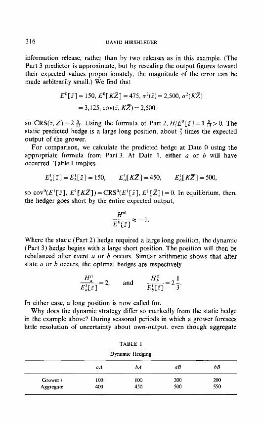
information release, rather than by two releases as in this example. (The Part 3 predictor is approximate, but by resealing the output figures toward their expected values proportionately, the magnitude of the error can be made arbitrarily small.) We find that

E”[Z] = 150, E’[KZ] = 475, o*(F) = 2,500, a’(Kz)

= 3,125, cov(5, Kz) = 2,500,

so CRS(& 2) = 2 & Using the formula of Part 2, H/p[Z] = 1 A> 0. The static predicted hedge is a large long position, about $ times the expected output of the grower.

For comparison, we calculate the predicted hedge at Date 0 using the appropriate formula from Part 3. At Date 1, either a or b will have occurred. Table I implies

EL[Z] = E;[z] = 150, EpLzT] = 450, Epz] = 500,

so cov”(E’[~], E’[KZ]) = CRS’(E’[?J, E’[z]) = 0. In equilibrium, then, the hedger goes short by the entire expected output,

Where the static (Part 2) hedge required a large long position, the dynamic (Part 3) hedge begins with a large short position. The position will then be rebalanced after event a or b occurs. Similar arithmetic shows that after state a or b occurs, the optimal hedges are respectively

Hf

E$] = 2’ and

H;f 1 m=23.

In either case, a long position is now called for. Why does the dynamic strategy differ so markedly from the static hedge

in the example above? During seasonal periods in which a grower foresees little resolution of uncertainty about own-output, even though aggregate

Grower i Aggregate

TABLE I

Dynamic Hedging

aA bA aB bB

100 100 200 200 400 450 500 550


uncertainty is being resolved, a short hedge is appropriate. Conversely, when the individual grower has high uncertainty resolution compared to the rest of the market (after 8’ occurs, in the example), a long hedge is taken. Dynamic futures trading strategies have been examined previously in both continuous time [3, 14, 8, 93 and discrete time models [ 16, 11. However, none of these papers have noted the impact on hedging of differing rates of information arrival about a grower’s own output versus aggegrate output.

[ 141 assumes an exogenous process for prices and one consumption good; it finds that if prices remain variable after output uncertainty is resolved, growers will hedge short. [IS, 91 provide closed-form solutions for optimal hedging strategies in continuous time settings with a single consumption good under a variety of objective functions. [16] solves a discerete time optimization problem.

[l] analyzes hedging, daily resettlement and price volatility in a discrete time mean-variance model. It shows that a grower’s optimal hedge depends on the correlation of different grower’s outputs during the holding period. Defining an overhedge as a short position larger in absolute magnitude than expected output, they maintain that “In an extreme case we might find a rational agent who underhedges at one point and overhedges at a later point.“”

Proposition 2 shows that a much more extreme outcome, the reversal of a full short sale of futures to a long purchase of futures, will occur as a typical case, so long as news arrives at different times for different growers. This is because it is not just correlation, but the rate of information arrival about different growers’ outputs that determines a grower’s optimal hedge. The resolution of uncertainty about other growers’ outputs translates through market clearing into information arrival about price, and the grower’s hedging position is based on his expected output and how his output covaries with price.

The variation in the optimal hedge is brought about by changing relative magnitudes of price risk versus quantity risk that a grower faces in different seasonal periods. In periods in which a grower faces predominantly price risk (news about others’ outputs), a short position is called for, while in periods in which he faces predominantly quantity risk (news about own output), a long position is appropriate. This intuition extends that of the single-event case: having low or high temporary uncertainty resolution is like having, temporarily, a low or (absolutely) high CRS with the aggregate. At Date 0 the grower foresees that 0, conveys no information whatsoever about the size of his own crop, so that his CRS’= 0, leading

*’ Their example (p. 260) is based on a market in which two substitute crops are positively correlated during the early growing season, and negatively correlated later.


to a short position. As commodities such as grains typically have harvest times that differ by location, resolution of uncertainty predictably takes place earlier in some regions than others.

The static hedge lies between the dynamic hedges predicted for Date 0 and for Date 1. Ignoring the structure of information arrival by applying a static model to a dynamic setting in some sense averages out dynamic hedging effects, which may yield a very poor description of behavior This is much like the distinguished attorney who believed that since, early in his career, he lost some cases he should have won, and later, won some cases he should have lost, that on average justice was done.

2.3. Stochastic Numeraire Endowment and Demand Shocks

The preceding section assumed that the primary source of uncertainty for the market was about the size of the crop. However, for some commodities shocks to demand are of greater importance than shocks to supply. For such commodities, a typical producer primarily faces price risk rather than quantity risk. The standard view is that in the absence of a bias in the futures price, a seller who faces price risk but not quantity risk will sell the commodity short (see, e.g., [ 17, 5, 15, 281). However, I show here that even if output is non-stochastic and the futures price is unbiased, the effect of demand shocks on optimal hedging depends critically on the source of the shift in demand. If demand shocks arise from stochastic output of all-other-goods (N), then a grower with non-stochastic output of the commodity (Z) may prefer to remain unhedged, or even hedge long, rather than hedging short as conventionally predicted.

I now assume that the aggregate endowed quantity of the numeraire N is stochastic, and that each grower possesses a non-stochastic endowment of the commodity he produces 2. The optimal hedging position in this setting is described by the following Proposition.

PROPOSITION 3. If consumers and producers have non-stochastic output of Z, but may have stochastic output of the numeraire, then:

(1) The optimal hedge at time j by individual i is

EJb+ ‘[ii/m] - EL+ ‘[fi/m]

> EL+’ [l/m] -E’,+‘[l/fl] ’ (11)

(2) If there is a single conclusive anticipated information arrival (m= 1) and E[Z] #O,

[l -CRS’(E’+‘[n], EJ+‘[~])]. (12)


(3) If there are many information events (m > 1) and E[fi] # 0, fp = [l -CRS’(E’+‘[n], E’+‘[m])]

+ O(a$ + o(o;) + O(o,ap). (13)

Although Proposition 3 is similar in form to Proposition 2, it has different economic implications. Consider the case of a grower whose endowment of N is proportional to aggregate N. Then CRS’(E’+ ’ [fi], Ej+ ‘[ml) = 1, implying that the grower optimally remains unhedged. Similarly, when the grower has a null endowment of N, fi E 0, (11) implies a null futures position. Thus, even though social variability of N creates price risk for the grower, he does not want to sell his output of 2 short on the futures market.

The grower faces a risk of a high price of corn when high aggregate N raises demand, and a low price of corn when the social output of N is low. But where the conventional analysis argues that this risk should be removed, here the grower retains his corn, which aligns his state-contingent levels of wealth with his planned consumption of N. In equilibrium, the spot price is proportional to the per capita quantity of all-other-goods N, and each individual’s planned consumption of N is also proportional to R. Thus, holding a bushel of corn is somewhat like holding a share in the “market portfolio”, in that it pays off the most when society is richest. The grower’s consumption levels are exactly aligned with those of pure consumers without any need for futures trading.**

Under more general preferences, an exact proportionality between the spot price and desired consumption expenditure will not hold. For example, under the modified logarithmic preferences U(n, z) = log(n - y) + 6 log(z), a poorer grower has a greater preference for (percentage) stability in his consumption of N than does a richer grower, and the spot market value of an additional unit of endowed Z in terms of N is more variable than Iv. It is not hard to show that under these preferences a grower whose endowment ti is proportional to the per capita endowment iV will hedge long or short depending on whether fi 2 m.

This analysis demonstrates that it is crucial to take into account general equilibrium considerations in making predictions about producer behavior in response to demand shocks. The traditional view that a producers will hedge short if his output is constant and he faces price risk is not necessarily valid if the source of price risk is uncertainty about aggregate

28 If the grower holds a non-stochastic positive endowment of N, then he is in a position of lower risk than the rest of society, and he will find it profitable to increase the sensitivity of his portfolio to aggregate wealth variations by taking a long futures position.


wealth. In reality, shifts in commodity demand are not perfectly correlated with shifts in aggregate wealth, so it is not possible to complete the market with only a commodity futures contract. However, so long as the demand for the commodity is affected by wealth shocks, variations in the value of producers’ output will still be correlated with society-wide wealth changes. Thus, whether a grower will want to hedge short to remove specific risk using commodity futures will depend on the cost of taking an appropriately time-varying position in stock index futures or mutual funds to regain participation in stock market swings.

3. CONCLUSION

Optimal hedging was analyzed in a setting in which (1) information about output arrives sequentially and at different rates for different growers, (2) individuals understand how the resolution of uncertainty about market price is related to news about outputs, (3) demand for the futures-traded commodity is determined as an optimizing consumption choice among different goods, and (4) individuals trade futures taking into account that the relative prices of the goods they consume are changing as anticipated new information arrives.

Use of such a general equilibrium framework yields a number of insights. The desire of a grower or consumer to hedge using futures arises from a discrepancy between his initial revenue or wealth distribution from his planned expenditure on the commodity and on other goods. In an effectively complete market with non-stochastic aggregate endowment of the numeraire, and either additively separable or common homothetic preferences, the planned consumption of other goods is constant, so that the goal of consumers and growers is to align their wealths with expenditure on the commodity

Optimal futures hedging positions are therefore determined by the factors that determine the initial alignment of growers’ revenues and expenditures, and the covariance of revenues with the payoff from holding a futures contract. With a single information arrival, these factors are (1) the correlation of a producer’s output with the aggregate, (2) the sensitivity of output to the environment (relative to other producers), and (3) demand price elasticity. Under unit elastic demand, growers with good poor- weather farms (whose output is relatively high when aggregate output is low) go short in futures; and growers with good fair-weather farms go long.

Furthermore, when information arrives sequentially growers tend to go long during seasonal periods when their output uncertainty is being resolved more rapidly than the aggregate, and short when their uncertainty is resolved less rapidly than the aggregate. This is of practical interest since


the timing of harvests typically depends on location. For example, the U.S. wheat crop begins in the southern part of the wheat belt, and moves north as the year progresses. Optimal hedging positions for the model with a single information arrival can be estimated using data on regional outputs, spot market price, the number of growers, and the total population size. For the model with many information events, regional crop forecasts can be used to estimate how seasonal revisions in output expectations affect optimal hedging positions.

The conventional view that growers facing pure price risk will hedge short is not necessarily valid. If demand shocks are caused by shifts in aggregate wealth, then a grower with non-stochastic output may maintain an unhedged position or take a long position in an unbiased futures market even though he faces price risk. This occurs because the value of his crop is correlated with social wealth, so that holding the commodity helps align his consumption of other goods with the social totals.

The most important conclusion of the paper is that it is a perilous error to select hedging positions as if information were going to arrive all at once, if in fact information arrives sequentially. Indeed, this could lead a grower to increase his risk by taking a short position during seasonal periods in which a long position is called for. A grower who can expect news about his own crop to arrive at a different time from that of others’ crops should take drastically different hedging positions from a grower in a market in which both sorts of news are expected to arrive at the same time.

APPENDIX

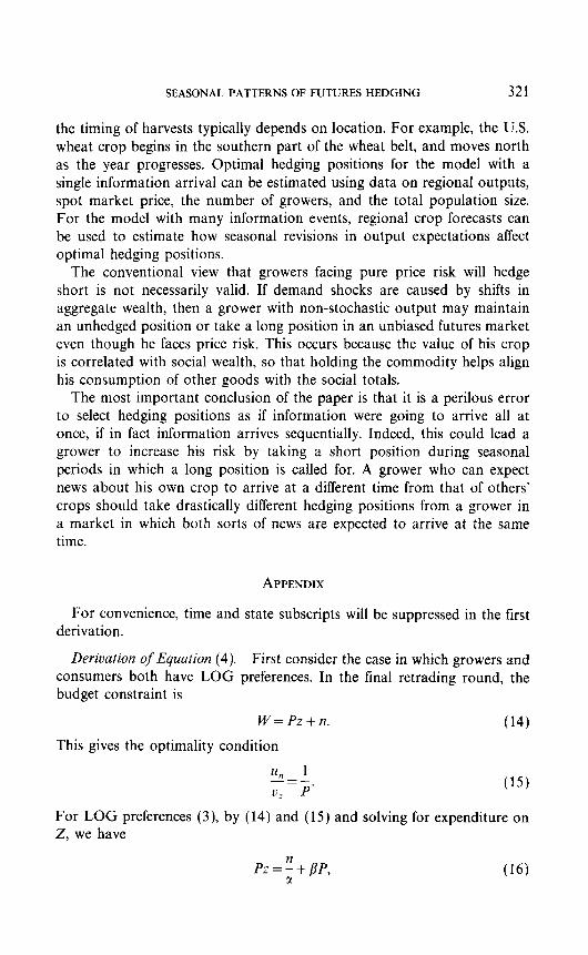
For convenience, time and state subscripts will be suppressed in the first derivation.

Deriuation of Equation (4). First consider the case in which growers and consumers both have LOG preferences, In the final retrading round, the budget constraint is

W= Pz+n.

This gives the optimality condition (14)

U” 1 -=- 0, P’ (15)

For LOG preferences (3), by (14) and (15) and solving for expenditure on Z, we have


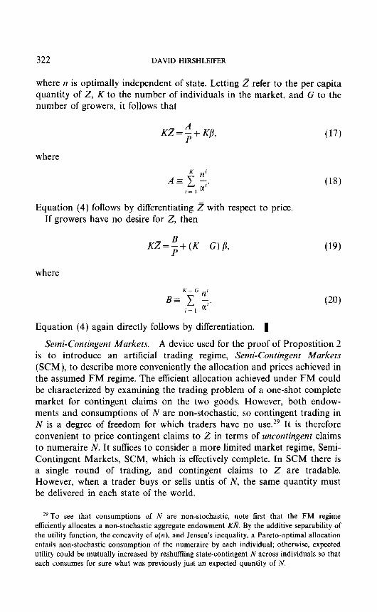
where n is optimally independent of state. Letting Z refer to the per capita quantity of 2, K to the number of individuals in the market, and G to the number of growers, it follows that

where

Equation (4) follows by differentiating Z with respect to price. If growers have no desire for Z, then

Kz=;+(K-G)j3,

where

(18)

(19)

K-G.1

BE c ;. (20) i=( a

Equation (4) again directly follows by differentiation. 1

Semi-Contingent Markets. A device used for the proof of Propostition 2 is to introduce an artificial trading regime, Semi-Contingent Markets (SCM), to describe more conveniently the allocation and prices achieved in the assumed FM regime. The efficient allocation achieved under FM could be characterized by examining the trading problem of a one-shot complete market for contingent claims on the two goods. However, both endowments and consumptions of N are non-stochastic, so contingent trading in N is a degree of freedom for which traders have no use.2g It is therefore convenient to price contingent claims to Z in terms of uncontingent claims to numeraire N. It suffices to consider a more limited market regime, Semi- Contingent Markets, SCM, which is effectively complete. In SCM there is a single round of trading, and contingent claims to Z are tradable. However, when a trader buys or sells untis of N, the same quantity must be delivered in each state of the world.

29 To see that consumptions of N are non-stochastic, note first that the FM regime efficiently allocates a non-stochastic aggregate endowment KN. By the additive separability of the utility function, the concavity of u(n). and Jensen’s inequality, a Pareto-optimal allocation entails non-stochastic consumption of the numeraire by each individual; otherwise, expected utility could be mutually increased by reshutlling state-contingent N across individuals so that each consumes for sure what was previously just an expected quantity of N.

SEASONAL PATTERNSOFFUTURES HEDGING 323

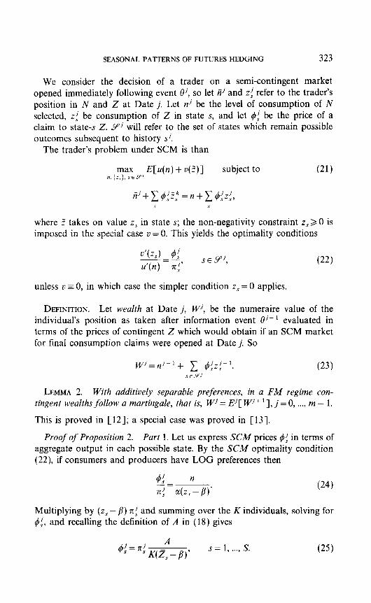
We consider the decision of a trader on a semi-contingent market opened immediately following event I?, so let tij and 2: refer to the trader’s position in N and Z at Date j. Let n-’ be the level of consumption of N selected, zi be consumption of Z in state s, and let 4: be the price of a claim to state-s Z. Yj will refer to the set of states which remain possible outcomes subsequent to history si.

The trader’s problem under SCM is than

where Z takes on value zs in state s; the non-negativity constraint z, 2 0 is imposed in the special case u = 0. This yields the optimality conditions

u’(z,) qq -- u’(n) - q’

SEYj, (22)

unless u z 0, in which case the simpler condition z, = 0 applies.

DEFINITION. Let wealth at Date j, W-‘, be the numeraire value of the individual’s position as taken after information event (II- ’ evaluated in terms of the prices of contingent Z which would obtain if an SCM market for final consumption claims were opened at Datej. So

Wj=nJ-l+ 1 @z;--‘. (23) se.‘pl

LEMMA 2. With additively separable preferences, in a FM regime contingent wealths follow a martingale, that is, Wj = Ej[ WJ+ ‘1, j = 0, . . . . m - 1.

This is proved in [12]; a special case was proved in [13].

Proof of Proposition 2. Part 1. Let us express SCM prices 4; in terms of aggregate output in each possible state. By the SCM optimality condition (22) if consumers and producers have LOG preferences then

4’ n “= 7r: cI(z, - j?)’ (24)

Multiplying by (zs - /?) $ and summing over the K individuals, solving for bi, and recalling the definition of A in (18) gives

A d:=+(~3-P). s = 1, . . . . s. (25)


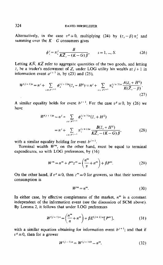
Alternatively, in the case vg= 0, multiplying summing over the K- G consumers gives

(24) by (z,- /?) 7~; and

B 4: = =i KZ, - (K- G) /j’ s = 1, . . . . s. (26)

Letting Kfl, KZ refer to aggregate quantities of the two goods, and letting Z, be a trader’s endowment of Z, under LOG utility his wealth at j+ 1 in information event ui+’ is, by (23) and (25),

A similar equality holds for event b j+‘. For the case ug = 0, by (26) we have

=nj+ 1 n;+lb B( 5, + If”) Kz, - (K- G) fi’ (28)

SEYJ+’

with a similar equality holding for event bj+‘. Terminal wealth W”, on the other hand, must be equal to terminal

expenditures, so with LOG preferences, by (16)

wm=.m+pmzm= (29)

On the other hand, if ug E 0, then z”’ = 0 for growers, so that their terminal consumption is

W” = nm. (30)

In either case, by effective completeness of the market, nm is a constant independent of the information event (see the discussion of SCM above). By Lemma 2, it follows that under LOG preferences

+ pP+ ““[P”], (31)

with a similar equation obtaining for information event b’+ i; and that if vg=O, then for a grower

w(i+l)a= w(i+l)b=,m (32)


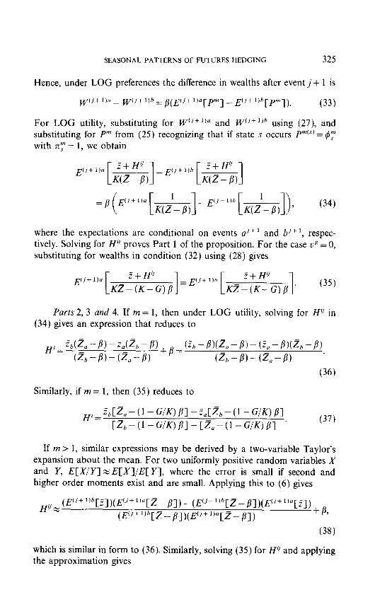
Hence, under LOG preferences the difference in wealths after event j + 1 is

wlj+ 1)~ _ W(J+ l)h = p(,ylj+ l)u[pm] -~(i+ l)b[pm]). (33)

For LOG utility, substituting for Wci+‘)’ and W(j+ ‘jh using (27), and substituting for P” from (25) recognizing that if state s occurs Pmts) = 4’: with rc”‘= 1 we obtain 3 )

where the expectations are conditional on events a’+’ and b’+ ‘, respectively. Solving for Hv proves Part 1 of the proposition. For the case vg = 0, substituting for wealths in condition (32) using (28) gives

Parts 2, 3 and 4. If m = 1, then under LOG utility, solving for H” in (34) gives an expression that reduces to

H’ = ~d-z - B) - Mb - PI (Z,-B)-(Z-P)

+B=(Z”-P)(~“-P)-(Zo-~)(tb-P) @,-BHzr8) .

(36)

Similarly, if m = 1, then (35) reduces to

Hi=ZbCZ,-(l-(;lK)P1-~,CZb-(l-GIK)P1 [.&-(l-G/K)p]-[Z,-(l-G/K)81 ’ (37)

If m > I, similar expressions may be derived by a two-variable Taylor’s expansion about the mean. For two uniformly positive random variables X and Y, E[X/Y] z E[X]/E[ Y], where the error is small if second and higher order moments exist and are small. Applying this to (6) gives

~j+1)6[~])(E(J+1)~[~-B])-(E(i+1)6[~_lj])(~(J+I)~[~])

(E(j+‘qZ- jjq)(E”’ ‘)a[T- p]) + A

(38)

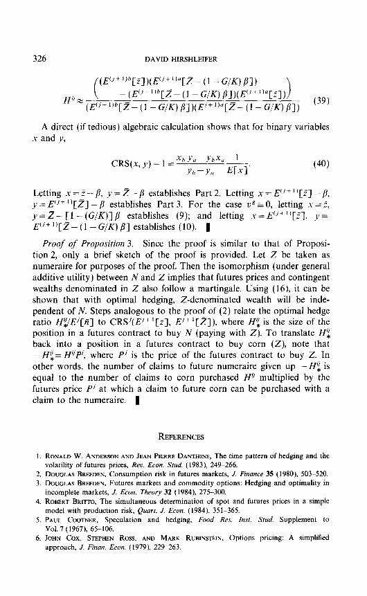
which is similar in form to (36). Similarly, solving (35) for H” and applying the approximation gives


-(E(j+‘lb[Z-(l -G/K)P])(E”+l’“[Z]) [Z-(l-G/K)fi])(E’+““[Z-(l-G/K)fi]) (39)

A direct (if tedious) algebraic calculation shows that for binary variables x and y,

CRS(x, u)- 1 = .xb +v, - )b.x, 1

- Yb-Y 0 E[Ixl’ (40)

Letting x = 5 -- p, y = 2 - /I establishes Part 2. Letting x = EtJ+ “[Z] - j?, y = E”“‘[Z] -/I establishes Part 3. For the case ug = 0, letting x = 5, y = z- [ 1 - (G/K)] j3 establishes (9); and letting .Y = E’j+ “[Y], y= E(j+ ‘)[z - (1 - G/K) fi] establishes (10). l

Proof of Proposition 3. Since the proof is similar to that of Proposi- tion 2, only a brief sketch of the proof is provided. Let Z be taken as numeraire for purposes of the proof. Then the isomorphism (under general additive utility) between N and Z implies that futures prices and contingent wealths denominated in Z also follow a martingale. Using (16), it can be shown that with optimal hedging, Z-denominated wealth will be independent of N. Steps analogous to the proof of (2) relate the optimal hedge ratio H$/Ej[5] to CRSj(E’+‘[Y], Ej”[.?]), where Hi is the size of the position in a futures contract to buy N (paying with Z). To translate Hi back into a position in a futures contract to buy corn (Z), note that -H’!= HvPj, where Pj is the price of the futures contract to buy Z. In other words, the number of claims to future numeraire given up -Hz is equal to the number of claims to corn purchased H” multiplied by the futures price Pj at which a claim to future corn can be purchased with a claim to the numeraire. g

REFERENCES

1. RONALD W. ANDERSON AND JEAN PIERRE DANTHINE, The time pattern of hedging and the volatility of futures prices, Rev. Econ. Stud. (1983), 249-266.

2. DOUGLAS BREEDEN, Consumption risk in futures markets, J. Finance 35 (1980), 503-520. 3. DOUGLAS BREEDEN, Futures markets and commodity options: Hedging and optimality in

incomplete markets, J. Econ. Theory 32 (1984), 275-300. 4. ROBERT BRI~TO, The simultaneous determination of spot and futures prices in a simple

model with production risk, Quart. J. Econ. (1984). 351-365. 5. PAUL COOTNER, Speculation and hedging, Food Res. Insr. Stud. Supplement to

Vol. 7 (1967), 65-106. 6. JOHN Cox, STEPHEN Ross, AND MARK RUBINSTEIN. Options pricing: A simplified

approach, J. Finan. Econ. (1979), 229-263.


7. DARRELL DUFFIE AND CHI-FU HUANG. Implementing Arrow-Debreu equilibria by continuous trading of few long-lived securities, Econometrica 54 (1985), 1161-1184.

8. DARRELL DUFFIE AND MATTHEW JACKSON, Optimal hedging and equilibrium in a dynamic futures market, J. Econ. Dvnam. Control, in press.

9. DARRELL DUFFIE AND HENRY R. RICHARDSON, “Mean-Variance Hedging in Continuous Time,” Stanford Graduate School of Business, January, 1989.

IO. FREDERICK L. A. GRAUER AND ROBERT H. LITZENBERGER, The pricing of commodity futures contracts nominal bond and other risky assets under commodity price uncertainty, J. Finance 34 (1979). 69-83.

11. DAVID HIRSHLEIFER, Residual risk, trading costs, and commodity futures risk premia, Rev. Finan. Stud. 1 (1988), 173-193.

12. DAVID HIRSHLEIFER, Hedging pressure and futures price movements in a general equilibrium model, Econometrica 58 (1990), 41 l-428.

13. JACK HIRSHLEIFER, The theory of speculation under alternative regimes of markets, J. Finance 32 (1977), 975-999.

14. THOMAS Ho, Intertemporal commodity futures hedging and the production decision, J. Finance 39 (1984). 351-376.

15. DUNCAN HOLTHAUSEN, Hedging and the competitive lirm under price uncertainty, Amer. Econ. Reu. 69, (1979), 989-995.

16. LARRY S. KARP. Dynamic hedging with uncertain production, ht. Econ. Rev. 29 (1988). 621-637.

17. JOHN MAYNARD KEYNES. “Some Aspects of Commodity Markets,” Manchester Guard. Commercial, European Reconstruction Series, March 29 1927): 784-786.

18. DAVID KREPS. Multiperiod securities and the efficient allocation of risk: A comment on the Black-Scholes option pricing model, in “The Economics of Information and Uncertainty” (J. J. McCall Ed.), Univ. of Chicago Press, Chicago, 1982.

19. ALLEN MARCUS AND DAVID MODEST, Futures markets and production decisions, J. Polit. Econ. 92 ( 1984), 409426.

20. RONALD I. MCKINNON, Futures markets. buffer stocks, and income stability for primary producers, J. Polk Econ. 75 (1967). 844-861.

21. DAVID M. G. NEWBERY AND JOSEPH E. STIGLITZ, “The Theory of Commodity Price Stabilization: A Study in the Economics of Risk,” Oxford Univ. Press, London, New York. 1981.

22. DAVID M. G. NEWBERY, Futures trading risk reduction and price stabilization, in “Futures Markets” (M. Streit, Ed.), Chap. 9, Blackwell, Oxford, 1983.

23. SCOTT RICHARD AND SURESH SUNDARESAN. A continuous time equilibrium model of forward prices and futures prices in a multigood economy, J. Finan. &on. (1981). 347-371.

24. JACQUES ROLFO. Optimal hedging under price and quantity uncertainty: The case of a cocoa producer, J. Polit. Eeon. 88 (1980). 100-l 16.

25. STEPHEN S. SALANT, Hirshleifer on speculation, Quart. J. Econ. 90 (1976), 667-676. 26. JON SALMON, “Consumption Risk, Storage, and the Extent of Futures Trading,” Ph.D.

Dissertation, UCLA, 198.5. 27. JOSEPH E. STIGLITZ, Futures markets and risk: A general equilibrium approach, in

“Futures Markets” (M. Streit. Ed.), Blackwell, Oxford, 1983. 28. HANS STOLL, Commodity futures and spot price determination and hedging in capital

market equilibrium, J. Finan. Quant. Anal. 14 (1979), 873-894. 29. STEPHEN J. TURNOVSKY, The determination of spot and futures prices with storable

commodities, Econometrica 51 (1983). 1363-1387.

Documents

Seasonal patterns of futures hedging and the resolution of output uncertainty