Embed Size (px)
Citation preview
1
Seasonal Decomposition of Cell Phone Activity Series and Urban Dynamics
Blerim Cici, Minas Gjoka, Athina Markopoulou, Carter T. Butts
2
Complex Urban Environments
o “Urban Dynamics”– Social & Economic
activities– Social Interaction
o Existing Methods to understand cities:– Surveys
• Expensive • Take time

3
Mobile Phone Activity & Urban Dynamics
o Mobile phone activity– Human Mobility– Large Population– No Extra Cost
o Aggregated CDR– Easier to Manage– Facilitates Data
Sharing
o What they tell about urban dynamics ?
4
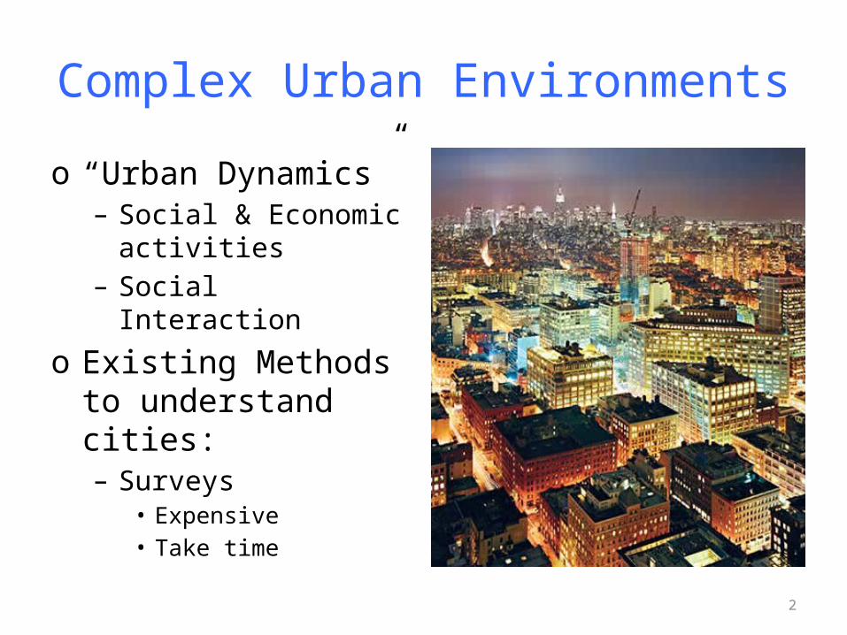
Milano CDR Dataset
o Big Data Challenge– Aggregate CDRs– Telecom Italia
o City:– Milano – 100x100 grid– Duration: 4 weeks
o Activity in grid-square:– Total Calls and SMS
Video snapshot for heatmap activity, Milan - Nov.1st 2013Dataset “Telecommunications – SMS, Call, Internet – MI”
5
Related Work
o CDRs: – Behavioral Traces
o Previous work:– Requires cultural knowledge:
• Weekdays vs. Weekends• e.g. [Soto et. al. HotPlanet, 2011]
– Systematic component only (e.g. typical days)• e.g. [Soto et. al. HotPlanet, 2011], [Toole et. al. UrbComp, 2012]
o Our work:– Principled method to extract systematic components– Go beyond systematic components
• Work with data previously considered as noise

6
Orig
inal -S
CS
FFT
High-a
mplitud
e
Decomposition Overview
Hypothesis:Regular Patterns
Hypothesis:Irregular Patterns
7
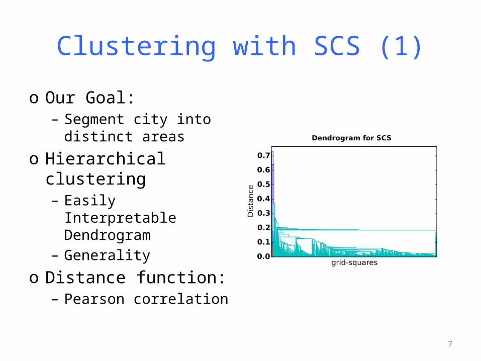
Clustering with SCS (1)
o Our Goal:– Segment city into
distinct areas
o Hierarchical clustering– Easily Interpretable
Dendrogram– Generality
o Distance function:– Pearson correlation

8
Clustering with SCS (2)
o Low-skewness segmentation:– Comparable sized clusters

9
SCS clusters vs. ground truth
*Ground truth from Milano Public data: Residential, Universities, Businesses, Bus stops, green areas, etc (http://dati.comune.milano.it/)
10
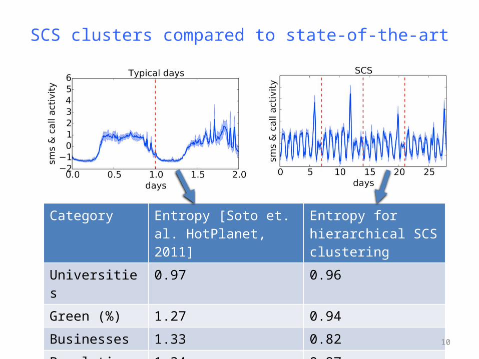
SCS clusters compared to state-of-the-art
Category Entropy [Soto et. al. HotPlanet, 2011]
Entropy for hierarchical SCS clustering
Universities 0.97 0.96
Green (%) 1.27 0.94
Businesses 1.33 0.82
Population 1.34 0.97
11
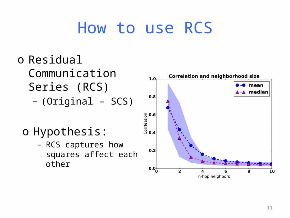
How to use RCS
o Residual Communication Series (RCS)– (Original – SCS)
o Hypothesis:– RCS captures how
squares affect each other

12
Maximal regions of mutual influence
o DiGraph, G(V,E):– Nodes: grid-squares– Edges:
• Lagged correlation (lag = 1)
• We keep only the strongest (5σ)
o Strongly connected components of G: – Areas subject to
mutual social influence

13
Validation of RCS 2
o Square-to-Square traffic matrix [T]– Source: Mi-to-Mi data– How much various
areas of the city talk to each other
o Quadratic Assignment Procedure (QAP)– Testing for correlation
with [T] against a null hypothesis
QAP test results SCS RCS
Correlation 0.05 0.27
Min random -0.018 -0.005
Mean random 0 0
Max random 0.011 0.004
14
Conclusion and Future Work
o RCS and SCS– Distinct Probes of Urban Dynamics– Obtained from the same underlying data.
o Future Work:– Apply technique to more cities– Apply technique to geo-social activity data (e.g.
Foursquare, Twitter)– Use current findings to activity prediction
15
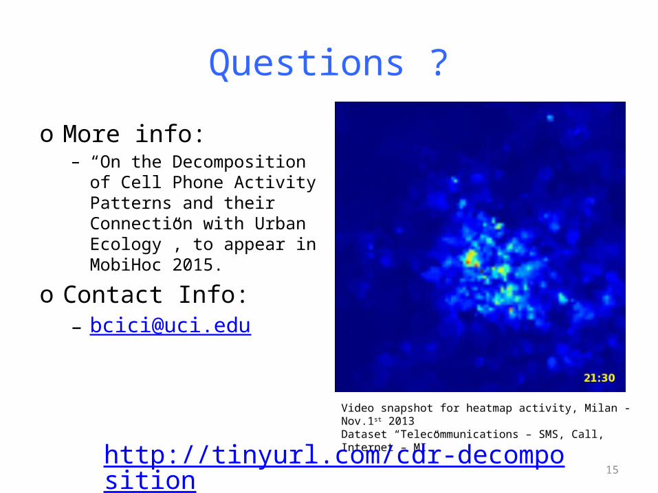
Questions ?
o More info: – “On the Decomposition of
Cell Phone Activity Patterns and their Connection with Urban Ecology”, to appear in MobiHoc 2015.
o Contact Info:– [email protected]
Video snapshot for heatmap activity, Milan - Nov.1st 2013Dataset “Telecommunications – SMS, Call, Internet – MI”
http://tinyurl.com/cdr-decomposition