University of Dayton University of Dayton

eCommons eCommons

Honors Theses University Honors Program

4-2017

Seasonal Changes in Physical, Chemical, and Biotic Factors in Seasonal Changes in Physical, Chemical, and Biotic Factors in

Silver Lake, Ohio Silver Lake, Ohio

Jacob J. Clancy University of Dayton

Follow this and additional works at: https://ecommons.udayton.edu/uhp_theses

Part of the Biology Commons

eCommons Citation eCommons Citation Clancy, Jacob J., "Seasonal Changes in Physical, Chemical, and Biotic Factors in Silver Lake, Ohio" (2017). Honors Theses. 102. https://ecommons.udayton.edu/uhp_theses/102

This Honors Thesis is brought to you for free and open access by the University Honors Program at eCommons. It has been accepted for inclusion in Honors Theses by an authorized administrator of eCommons. For more information, please contact frice1@udayton.edu, mschlangen1@udayton.edu.

Seasonal Changes in Physical,

Chemical, and Biotic Factors

in Silver Lake, Ohio

Honors Thesis

Jacob J. Clancy

Department: Biology

Advisor: P. Kelly Williams, Ph.D.

April 2017

Seasonal Changes in Physical,

Chemical, and Biotic Factors

in Silver Lake, Ohio

Honors Thesis

Jacob J. Clancy

Department: Biology

Advisor: P. Kelly Williams, Ph.D.

April 2017

Abstract The chemical makeup of a body of water can vary greatly depending on what kind of lake it is, the time of year and what kind of runoff enters the water. There are many abiotic factors that make up the water chemistry of a lake such as nutrient availability (Nitrogen and Phosphorous), pH, temperature, oxygen content and conductivity. Each of these factors plays important roles in the successes of many organisms that reside in the lake. The many species of zooplankton and phytoplankton thrive in different water chemistry conditions. Silver Lake is a unique lake in Ohio, because it was formed by a glacier and has no surface water inlets, it is spring-fed. Silver Lake has had no prior limnology studies conducted on it, so it is a novel system for this kind of study. Silver Lake plankton and chemistry data was compared to Lake Erie’s Western Basin and Grand Lake St. Marys, which have had harmful algal bloom problems in the past. These two lakes are considered eutrophic, and after close comparison with them, Silver Lake was determined to be a nutrient-poor oligotrophic lake.

Table of Contents

Abstract Title Page

Introduction 1

Materials and Methods 5

Results 9

Discussion 12

Conclusions 14

Acknowledgements 15

References 16

Figures 19

P a g e | 1

Introduction Background

Freshwater lakes and reservoirs are very important ecosystems for both the

humans that utilize them, and the abundance of other organisms that rely upon them for

life. These ecosystems are very biodiverse and support life at many different levels, from

fish down to the smallest microorganisms. The character of the ecosystem of a lake is

dependent upon many physical, chemical, and biological factors.

The abiotic factor of temperature is of vital importance to every organism that

lives in a lake. Organisms of interest to this study that are living in the lake are

poikilothermic (heterotherms) organisms, which means that they do not regulate their

own body temperature. The temperature of the body of water is one of the most important

factors of the ecosystem because temperature effects organism metabolism, which in turn

effects temperature tolerance and biotic competition. Lakes undergo a seasonal change in

temperature resulting in thermal stratification based on physical water qualities. Certain

lakes that have two annual circulations are referred to as dimictic lakes (two mixes a year,

one in the fall and one in the spring). Seasonal temperature changes in the lake relate to

species presence, abundance, and lake-wide productivity changes. In the summer time,

dimictic lakes are stratified because there is very little mixing and the top layer of water

is very warm, while under a certain depth, called the thermocline, the temperature drops

considerably. The warm, top layer stays at the top getting warmer, because water is less

dense when it is warm. For this reason, the cold water moves to the bottom, because

water is more dense when it is cold, until reaching its most dense at 4 °C (Brönmark &

Hansson, 2005). Temperature is a very important physical factor, because different

phytoplankton and zooplankton species have different thermal tolerances. Zooplankton

species also vary seasonally based on physical and biotic factors. This makes temperature

a very useful factor to measure and analyze, not only to determine how the lake

functions, but also to predict and determine the distribution of organisms like

zooplankton and phytoplankton.

The pH of a system is a vital factor to the overall health of the lake and the

organisms in the lake. The pH can vary dramatically if the alkalinity, or buffering

capacity, of a body of water is low. Anything from acid rain to the bicarbonate-carbon

P a g e | 2

dioxide equilibrium to the amount of photosynthesis and respiration occurring in the lake

can alter the levels of pH. The pH measurements can be informative about the geology of

the lake and how water is entering the lake ecosystem. The measure of pH is an important

factor because extreme pH levels, either too high or too low can cause health and

reproductive issues in a lot of the planktons and higher organisms in the lake. If a body of

water is left at extreme levels for an extended period of time, it can restructure the lake

ecosystem by allowing different phytoplankton species to thrive (Brönmark & Hansson,

2005).

Conductivity is the measure of how well a body of water carries an electrical

charge, which is another important physical factor that is really a measure of the

dissolved solids (ions) in the water. The concentration of ions in a body of freshwater

have to remain at low levels for the organisms to have high levels of fitness in that

environment. Many freshwater organisms must maintain a hypertonic inside of their

bodies relative to the water. These organisms spend energy on osmoregulation to prevent

water uptake and ion loss. If the amount of ions, usually calcium and carbonate, in the

water is altered by too much, these organisms must spend more of their energy on

osmoregulation. This extra expenditure of energy takes energy away from growth and

reproduction in these organisms. These organisms can survive salinity changes, but their

overall fitness decreases dramatically because they are less able to grow and reproduce.

Oxygen availability, mostly referred to as dissolved oxygen (DO), is a chemically

measured factor because many organisms that are living in freshwater lakes rely on

oxygen to carry out aerobic metabolism. Oxygen can be absorbed atmospherically into

the water, but most of the oxygen comes from photosynthesizing plants and

phytoplankton. Oxygen levels fluctuate greatly throughout the day and may decrease

dramatically at night, because there is only aerobic respiration at night, using oxygen and

creating carbon dioxide. A good level of oxygen saturation indicates a healthy ecosystem.

Super saturation of oxygen can occur with algal blooms but at night significant oxygen

depletion may occur. The overgrowth of algae like this can be caused by the abundance

of nutrients like phosphates and nitrates in the lake.

Phosphorous is usually the limiting element for growth in phytoplankton

(according to the Redfield Ratio, 106:16:1 C:N:P, which gives the optimal growth ratio,

P a g e | 3

any variation in the ratio indicates nutrient limitation), because of its generally low

concentrations in freshwater. When phosphorus is abundant it can be the best growth

factor, often causing overgrowth of algae. According to this study, (Maberly, King, Dent,

Jones, & Gibson, 2002), masses of phytoplankton can be just as likely to be limited by

nitrogen as phosphorous depending on the location or situation, but can especially happen

in unproductive lakes.

One way in which lakes can be described is by their nutrient contents, and as a

result, their overall productivity. Nutrients, such as nitrogen-containing molecules like

nitrate, phosphorous-containing molecules, magnesium, and calcium are all vital to the

growth and success of lake plants and plankton species. A lake that is rich in these

nutrients is considered a eutrophic lake. This kind of lake has a lot of phytoplankton,

algae, and aquatic plants, which leads to high levels of production. This also leads to very

opaque and murky water, which does not allow light to penetrate deep into the lake.

Oligotrophic lakes are lakes that are considered to be low in nutrient concentration. Low

nutrient concentration usually results in very clear water due to the low levels of

production from the low plankton abundance. Phosphorous is the nutrient that is usually

measured to determine whether a lake is oligotrophic or eutrophic. This is the nutrient of

interest because it is usually the limiting nutrient in phytoplankton growth. Since it is the

limiting nutrient, phosphorous is usually the determining factor for production in a lake.

Nitrogen is also an important nutrient for organismal growth in a lake. Nitrogen is not

often the limiting nutrient, but when there are high enough levels of pollution

(phosphorus) in the lake, then nitrogen can become limiting. High phosphorous and

nitrogen levels can lead to an overabundance of algae and a drastic increase in primary

production.

Plankton species, both zooplankton and phytoplankton are vital organisms to a

lake ecosystem. They play important roles in the food web and production in the lake. In

a study, their food web importance was tested when phosphorous load increased in a lake

and GPP (Gross Primary Production) rose from increased phytoplankton abundance,

large zooplankton dominated the ecosystem by feeding on the available algae (Cole,

Pace, Carpenter, & Kitchell, 2000). These organisms can also be used quite effectively as

P a g e | 4

indicators for the health or characteristics of a certain ecosystem. Just like any other

organism, they all occupy niches in which they are better able to survive and compete.

Inputs of nutrients (as mentioned previously) into lakes and reservoirs can have

large effects on the plankton, sometimes causing algal blooms when the nutrient levels

are high enough. These nutrients mainly get into the lakes and reservoirs from agriculture

and livestock. The fertilizer is washed away into streams which carry the nutrients

through the watershed into the lakes (Beaver et al., 2014; Hoorman et al., 2008; Michalak

et al., 2013). If the conditions are right and certain cyanobacteria bloom, it is referred to

as a HAB (Harmful Algal Bloom). Cyanobacteria that have caused issues in Ohio are

Anabaena, Microcystis, and Planktothrix. Some species of these organisms create a toxin

known as Microcystin, which is a hepatotoxin and can be very dangerous at high levels

(Millie et al., 2009; Dumouchelle, D.H., and Stelzer, E.A., 2014). Within the lake itself,

the zooplankton may also be harmed by the toxins as one study suggests (Freitas,

Pinheiro, Rocha, & Loureiro, 2014), or that they may have increased resistance to the

toxins if they have been exposed prior (Gustafsson & Hansson, 2004). These could both

have food web implications for higher predators.

Silver Lake in New Carlisle, Ohio is a unique Ohio lake because it is not man-

made nor does it have a surface water inlet. The lake is surrounded on three sides by high

ridges, which prevents surface water from streams or rivers from entering the lake. On

the fourth side is low ground, where the overflow of the lake forms a wetland. This lake

was formed by glacial activity and sits on top of glacial gravel and sedimentary rock. The

lake is fed by groundwater springs from under the lake. No previous study has been

conducted on the water chemistry, algae, and zooplankton abundances and impacts on the

lake.

Two other lakes in Ohio were selected to compare to Silver Lake to show how

different bodies of water are structured. The two lakes, Grand Lake Saint Marys (GLSM)

and Lake Erie (Western Basin) are shallow, very warm in the summer and are notoriously

prone to algal blooms (Davis, Koch, Marcoval, Wilhelm, & Gobler, 2012; Hoorman et

al., 2008; Kutovaya et al., 2012; Michalak et al., 2013; Millie et al., 2009; Ohio, 2010). In

contrast to Silver Lake, these lakes have a lot of surface water and surface runoff input

directly into the lakes. Data show that the nutrients in these lakes are in high abundance

P a g e | 5

and that this is a result of these inputs. Data from recent studies also show very high

concentrations and abundance of algae and zooplankton (Allinger & Reavie, 2013;

Michalak et al., 2013; Steffen, Zhu, McKay, Wilhelm, & Bullerjahn, 2014). These studies

attribute the levels of plankton to the high nutrient levels from the intake of agriculture

runoff through the surface water.

This study is a comparison of lakes with completely different characteristics. This

is an important study to conduct, because studying how the health of a lake is influenced

by what is input from different sources can help more fully understand what is occurring.

A lake such as Silver Lake is a useful ecosystem to study because surface water input

does not have any effect on the characteristics of the lake. This fact allows for the health

of the lake to be completely dependent upon the spring/ground water inputs. This is

compared to the other Ohio lakes, whose health is determined by the surface water inputs

from the surrounding areas. The hypotheses for this study are:

H1: There will be low nutrient abundance in Silver Lake when compared to the

other two lakes due to lake conditions, lake geology, and lake inputs.

H2: There will be less algae abundance and lower zooplankton abundance in

Silver Lake than the other two lakes due to lake conditions and lack of nutrients.

These are important determinations to make because the presence and abundance of algae

and zooplankton are good indicators of the kind and the health of the physical

environment of the lakes.

Materials and Methods Field Collection Data and samples were collected on six different occasions in the span of

September through November of 2016. All of the data and samples were collected from

the side of a boat in open water in Silver Lake. A buoy or marker was not set, so the same

location on the lake was not sampled each time. With the lake not being very large, a

position in very open water was chosen each sampling date and assumed to be

representative of the whole lake. The boat was also not equipped with large enough

P a g e | 6

anchors to hold it steady in windy conditions, which may have resulted in some drifting

away from the original position.

In order to test the lake for light penetration and water clarity, a Secchi disk was

used. The disk was lowered off of the side of the boat and into the water. The researcher

must watch the Secchi disk sink into the water and stop the descent immediately when

the disk becomes no longer visible. The depth measurement, in meters, was taken when

the Secchi disk was at a depth where it had just faded out of sight. Secchi depth is also an

indirect measure of primary production, indicating how deep in the water photosynthesis

can occur.

Physical or abiotic properties of the lake was another parameter where data was

collected in the field. A Yellow Springs Instruments Multi-Parameter Display System

(YSI 650 MDS) electronic probe was used to collect physical data: temperature (°C),

dissolved oxygen (DO) (mg/L), chlorophyll (mg/L), pH, and conductivity (µS/cm). This

probe was lowered down into the water off of the side of the boat, stopping at each meter

(m) of depth until the bottom of the lake was reached. Each meter was sampled in order

to obtain the profile of the entire water column for each physical parameter.

Plankton samples were also taken on the six sampling dates. While anchored in

the same location where the physical data were collected, quantitative plankton samples

were also collected. A vertical plankton net was used which allows sampling at certain

depths by having the ability to close the opening of the net at the desired depth. The

plankton are collected in the net by reaching a desired depth, then pulling the net

vertically upwards through the water column until the shallower desired depth is reached.

Once the shallower depth is reached, a “messenger” (a metal weight) is sent down the

line, which disconnects the line from the opening and effectively closing the net. When

the net is closed, it can be lifted up through the water without capturing any additional

organisms. The dimensions of this net included a circular opening with a 12 cm diameter,

and since the net was pulled one meter at a time, a height of 1 meter (100 cm). Each

sampling day, plankton were collected five times (five vertical pulls) at each of the

following 1 meter depth intervals: 5-4 m (below the surface), 4-3 m, 3-2 m, 2-1 m, and 1-

0 m. A total of 25 one-meter pulls were carried out each sampling occasion. The samples

from each depth were filtered into plastic vials. Each sample was preserved with 5%

P a g e | 7

Formalin and 95% Ethanol and then diluted so that the volume of each vial was 30 ml.

The samples were then stored for further analysis.

Qualitative plankton samples were taken on each of these dates. To collect these

samples, a plankton was towed behind the boat, along and just under the surface of the

water. These samples were kept in plastic vials and preserved with Formalin and 95%

Ethanol. These six samples were taken so that the plankton can be qualitatively assessed

for each time period. These were important samples to take to be practiced at identifying

the different zooplankton and phytoplankton taxa and to know what to expect to be

present on each date when looking at the quantitative plankton samples.

Plankton Data Collection and Analysis

The zooplankton and phytoplankton were analyzed using microscopes. The

zooplankton were assessed using a dissecting microscope under 40x magnification. The

30 ml quantitative samples were stirred to ensure even distribution of the organisms

throughout the container. One ml was drawn out of the sample with a pipette and placed

on to a Sedgewick rafter cell. Once on the slide, the different zooplankton taxa were

identified and counted. The different zooplankton were identified as adult Copepods,

larval Copepods, Cladocerans, or Rotifers using a series of published keys (Eddy,

Hodson, Underhill, Schmid, & Gilbertson, 1982; Needham & Needham, 1962; Thorp &

Covich, 2010). This process was done twice for each of the 30 total quantitative samples

(2 ml).

The phytoplankton analysis was also done under a microscope, but since they are

much smaller in comparison, higher magnification and smaller subsamples were needed.

The phytoplankton were assessed under a compound light microscope at 100x

magnification. The quantitative samples were thoroughly stirred so that there was even

organism distribution in the container. A pipette was used to draw out and place 0.14 ml

onto a microscope slide with a cover slip. The phytoplankton were analyzed by being

identified and counted. The different phytoplankton were identified to the lowest

classification possible, usually family or genera using a series of published keys

(Graham, Wilcox, & Graham, 2009; Needham & Needham, 1962; Reynolds, 1984;

Smith, 1933). One slide was made for each of the 30 samples. Ten unique microscope

P a g e | 8

fields of vision were picked out on each microscope slide to be analyzed for presence and

abundance of phytoplankton taxa.

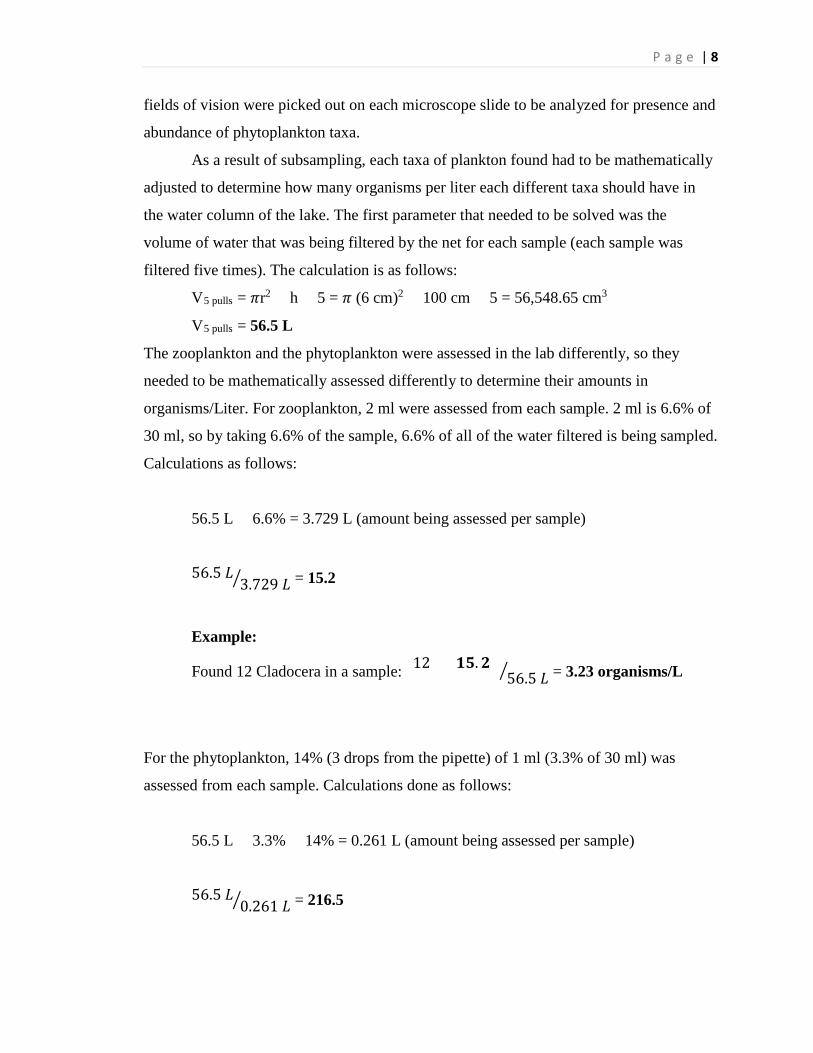
As a result of subsampling, each taxa of plankton found had to be mathematically

adjusted to determine how many organisms per liter each different taxa should have in

the water column of the lake. The first parameter that needed to be solved was the

volume of water that was being filtered by the net for each sample (each sample was

filtered five times). The calculation is as follows:

V5 pulls = 𝜋𝜋r2 × h × 5 = 𝜋𝜋 (6 cm)2 × 100 cm × 5 = 56,548.65 cm3

V5 pulls = 56.5 L

The zooplankton and the phytoplankton were assessed in the lab differently, so they

needed to be mathematically assessed differently to determine their amounts in

organisms/Liter. For zooplankton, 2 ml were assessed from each sample. 2 ml is 6.6% of

30 ml, so by taking 6.6% of the sample, 6.6% of all of the water filtered is being sampled.

Calculations as follows:

56.5 L × 6.6% = 3.729 L (amount being assessed per sample)

56.5 𝐿𝐿

3.729 𝐿𝐿� = 15.2

Example:

Found 12 Cladocera in a sample: (12 × 𝟏𝟏𝟏𝟏.𝟐𝟐 )56.5 𝐿𝐿� = 3.23 organisms/L

For the phytoplankton, 14% (3 drops from the pipette) of 1 ml (3.3% of 30 ml) was

assessed from each sample. Calculations done as follows:

56.5 L × 3.3% × 14% = 0.261 L (amount being assessed per sample)

56.5 𝐿𝐿0.261 𝐿𝐿� = 216.5

P a g e | 9

Example:

Found 39 Tribonema in a sample: (39 × 𝟐𝟐𝟏𝟏𝟐𝟐.𝟏𝟏)56.5 𝐿𝐿� = 149.4 organisms/L

Results Physical Data Silver Lake was sampled for physical and biological data on six different dates in

the autumn of 2016. The first measurements that were done were to assess water clarity

and light penetration in the water column. This measurement was taken by using a Secchi

disk. In the beginning of autumn the Secchi disk measurement was 5.8 meters. In early

October, the clarity depth dropped down to 4.5 then 4.42 meters. The Secchi disk clarity

depth rose once more to 5.45 meters toward the end of October before dropping down to

3.6 and 3 meters respectively in the last two sampling dates of this study.

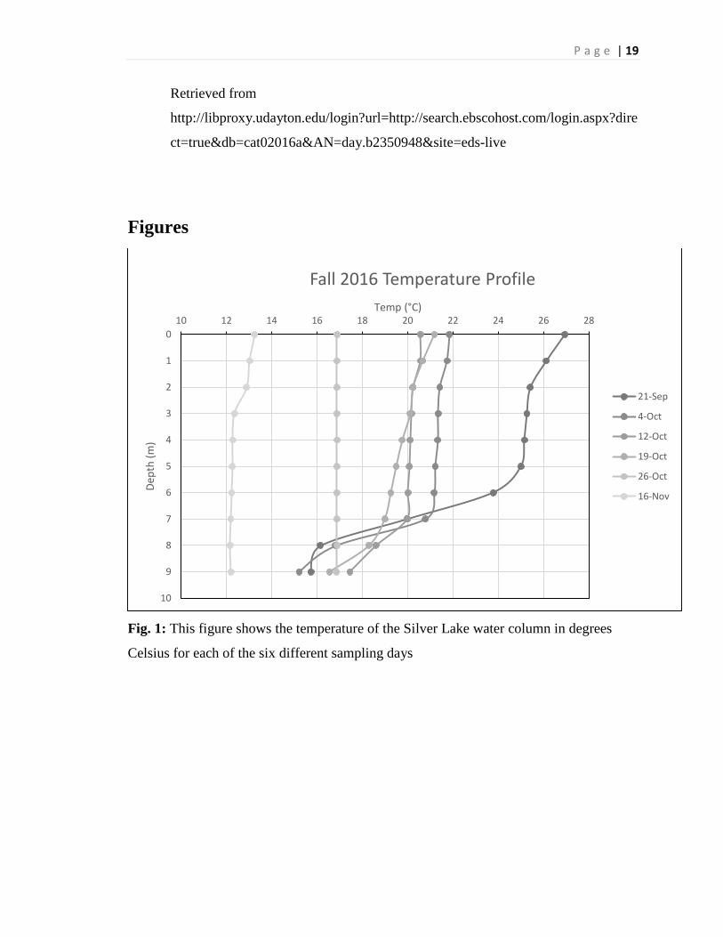
Temperature was a physical measurement that changed a lot from start to finish

over the course of this study. On September 21st, the water column was still stratified and

the temperature on the surface of the lake was 26.93 °C, while the bottom of the lake was

much colder at 15.73 °C. There is a thermal stratification witnessed in the next three

sampling periods, but to a lesser degree than in September. From October 4th through

October 19th the top few meters of the water column measured from 21.84 °C to 20.16

°C. The bottom layer of the late across these dates still showed thermal stratification,

because the temperatures ranged from 15.2 °C to 17.5 °C. The thermal stratification is

less pronounced here, but is still present. At the end of October a mixing event is seen as

the water gets cold enough. The entire lake became 16.9 °C from top to bottom. By

November 16th, the whole lake was still one temperature throughout, but got colder down

to 12.8 °C at this point in the year (Figure 1).

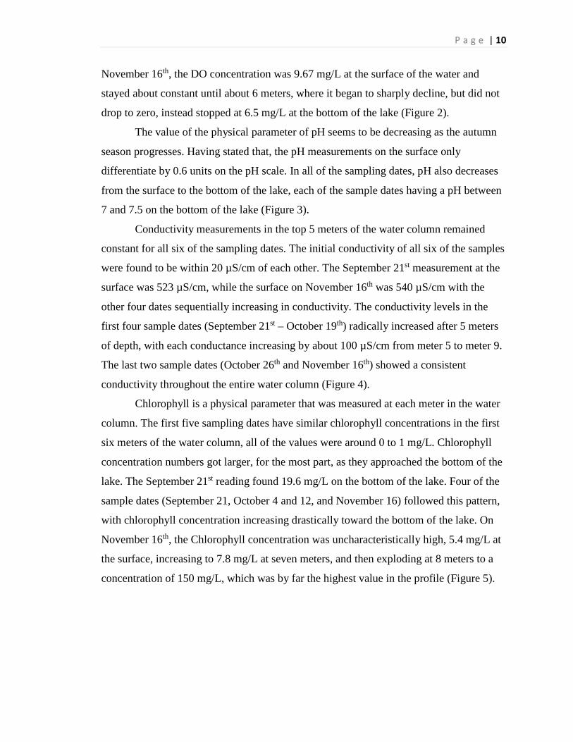
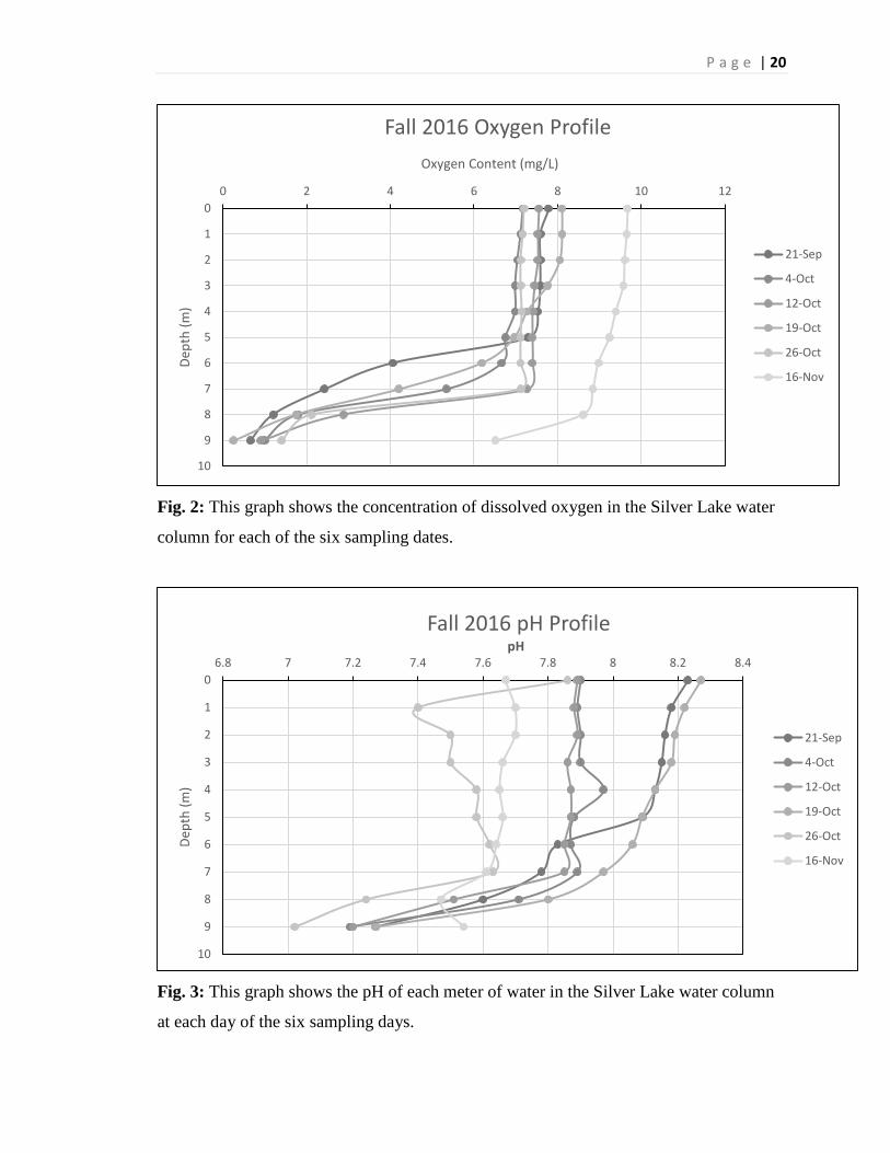
The amount of dissolved oxygen in the lake stayed relatively constant throughout

the autumn, but had a characteristic falling off towards the bottom of the lake. The first

five sample days had very similar values for dissolved oxygen content. From the 21st of

September through the 26th of October, the lake had a DO content ranging from 7.2 mg/L

to 8.1 mg/L at the surface with constant values as depth increased to about 6 meters deep.

After six meters, the oxygen concentration plummeted to almost zero in all 5 cases. On

P a g e | 10

November 16th, the DO concentration was 9.67 mg/L at the surface of the water and

stayed about constant until about 6 meters, where it began to sharply decline, but did not

drop to zero, instead stopped at 6.5 mg/L at the bottom of the lake (Figure 2).

The value of the physical parameter of pH seems to be decreasing as the autumn

season progresses. Having stated that, the pH measurements on the surface only

differentiate by 0.6 units on the pH scale. In all of the sampling dates, pH also decreases

from the surface to the bottom of the lake, each of the sample dates having a pH between

7 and 7.5 on the bottom of the lake (Figure 3).

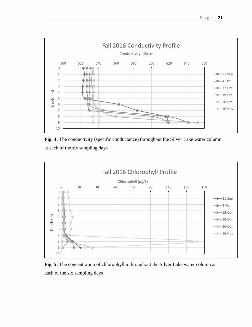
Conductivity measurements in the top 5 meters of the water column remained

constant for all six of the sampling dates. The initial conductivity of all six of the samples

were found to be within 20 µS/cm of each other. The September 21st measurement at the

surface was 523 µS/cm, while the surface on November 16th was 540 µS/cm with the

other four dates sequentially increasing in conductivity. The conductivity levels in the

first four sample dates (September 21st – October 19th) radically increased after 5 meters

of depth, with each conductance increasing by about 100 µS/cm from meter 5 to meter 9.

The last two sample dates (October 26th and November 16th) showed a consistent

conductivity throughout the entire water column (Figure 4).

Chlorophyll is a physical parameter that was measured at each meter in the water

column. The first five sampling dates have similar chlorophyll concentrations in the first

six meters of the water column, all of the values were around 0 to 1 mg/L. Chlorophyll

concentration numbers got larger, for the most part, as they approached the bottom of the

lake. The September 21st reading found 19.6 mg/L on the bottom of the lake. Four of the

sample dates (September 21, October 4 and 12, and November 16) followed this pattern,

with chlorophyll concentration increasing drastically toward the bottom of the lake. On

November 16th, the Chlorophyll concentration was uncharacteristically high, 5.4 mg/L at

the surface, increasing to 7.8 mg/L at seven meters, and then exploding at 8 meters to a

concentration of 150 mg/L, which was by far the highest value in the profile (Figure 5).

P a g e | 11

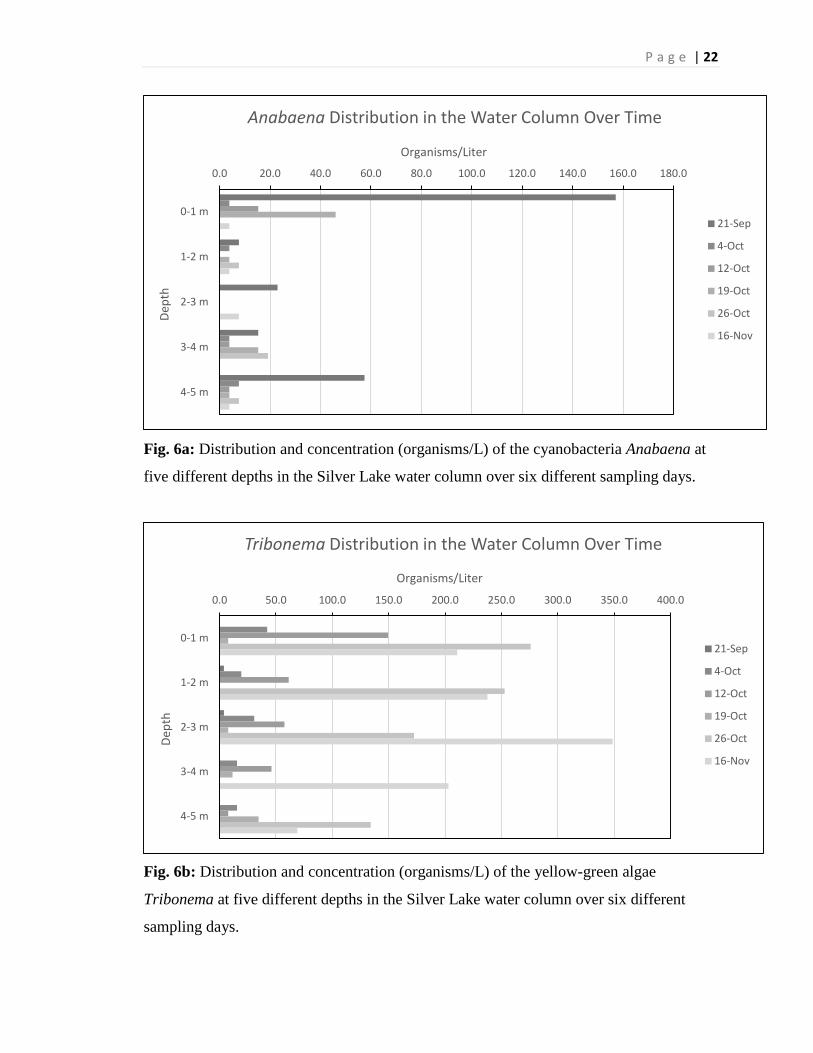
Biological Data Algae

The algae, or phytoplankton, were collected at different specific depths and

throughout the season. There were a total of seventeen different taxa of phytoplankton

that were identified in this study, but only three were abundant enough to do a sound

assessment of them. The three taxa that were identified were Anabaena, Tribonema, and

Microcystis. Anabaena was found to have a total mean abundance (across all depths and

time periods) of 14.8 organisms per liter. The genus Anabaena was very abundant early

in the season, September 21st, and higher in the water column, but decreased drastically

as the season went on and at deeper depths (Figure 6a). Tribonema was found to have a

total mean abundance of 80.6 organisms per liter. This genus of yellow-green algae was

abundant throughout the sampling depths and times, but increased dramatically at the end

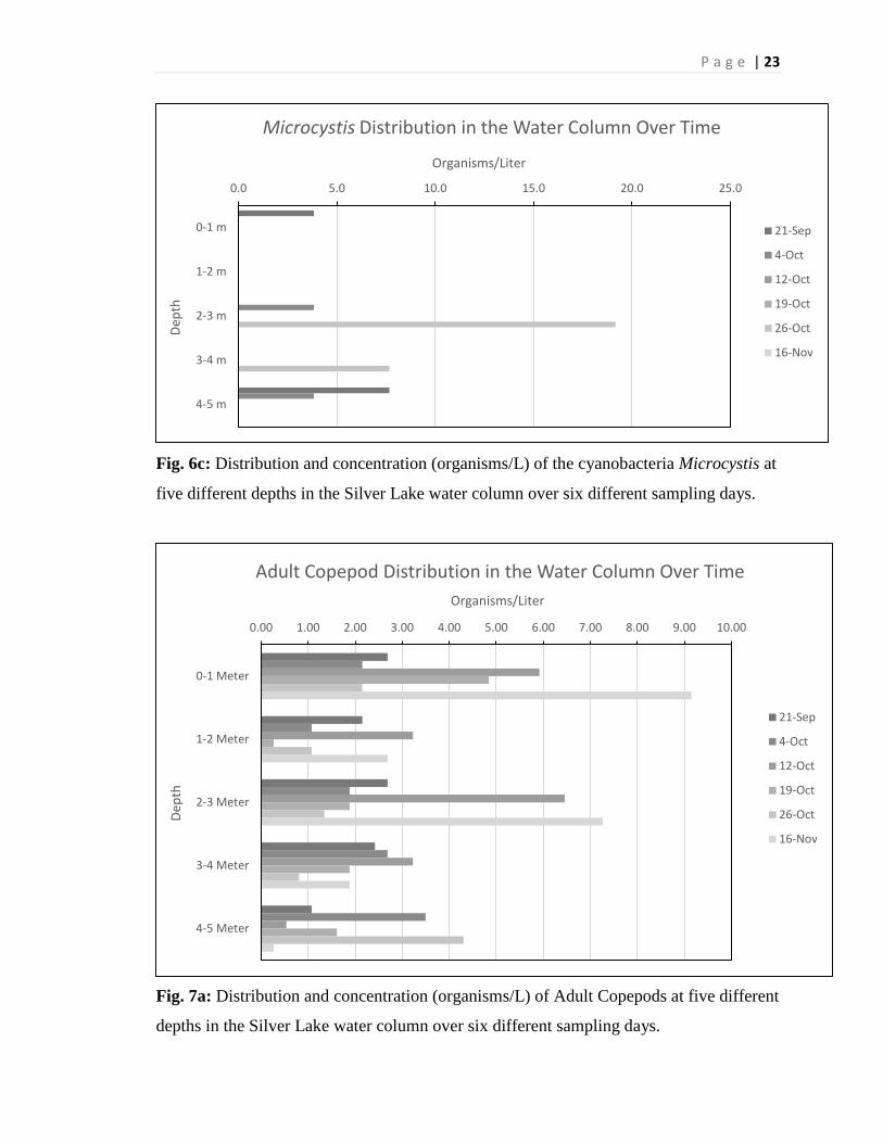
of the season across all depths (Figure 6b). The total mean abundance of Microcystis was

1.5 organisms per liter. Microcystis was very scarcely found in any of the sample depths

or times, and was actually not found in more samples than it was found in (Figure 6c).

Zooplankton

The zooplankton that were collected were identified into four different categories:

Adult Copepod, Larval Copepod, Cladocera, or Rotifer. These zooplankton were

analyzed in regards to two different parameters. They were collected and analyzed

according to the date in which they were collected and what depth they were collected in

the water column. The mean abundance of zooplankton that were collected was shown to

be 3.88 zooplankton per liter (rotifers left out due to their total mean of .11 rotifers per

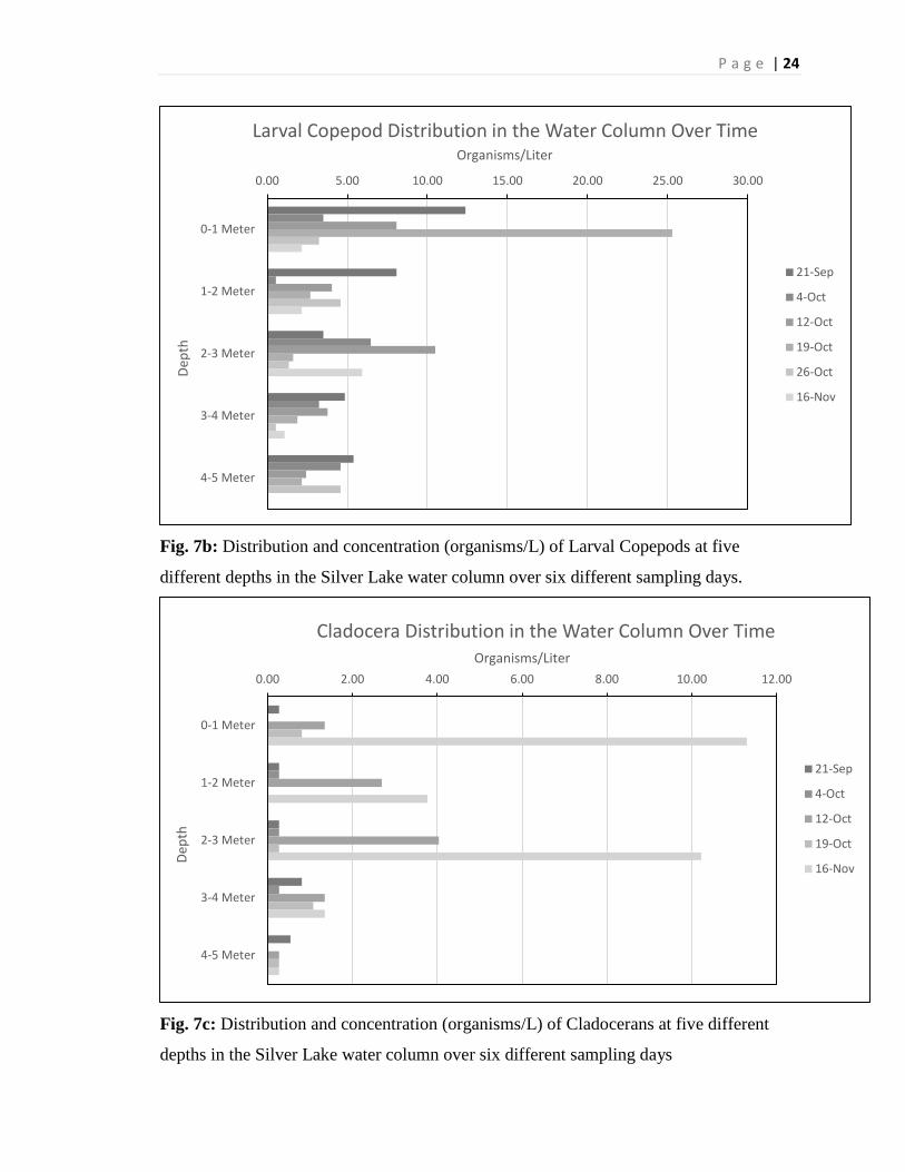
liter). Adult Copepods had a total mean abundance of 2.77 organisms per liter. Larval

Copepods had a total mean abundance of 4.68 organisms per liter. Cladocerans had a

total mean abundance of 4.19 organisms per liter. These data include samples across the

whole time frame and the entire range of depths that were sampled. The adult Copepods

do not have a clear correlation with either depth or progression of the season, but seem to

be more abundant in the first and the third meter of the water column later in the season

(Figure 7a). The larval Copepods do not seem to show a trend either, except for the first

meter, in which they are slightly more abundant (Figure 7b). The Cladocera show a very

P a g e | 12

high abundance late in the season, October 26th, throughout the entire water column

(Figure 7c).

Discussion The data collection and the assessment of this data from Silver Lake provide us

with a platform in which we may make comparisons to other bodies of water and the data

that have been analyzed about them.

Secchi disk depth is an important measurement that is taken of a lake. The

measurement gives relative information about the clarity of the water and therefore the

amount of primary production that occurs in the lake. In the study by Dumouchelle, D.H.,

and Stelzer, E.A., 2014, data gathered from GLSM by the USGS (United States

Geological Survey) and the OEPA (Ohio Environmental Protection Agency) show that

Secchi Disk depths show a range of 0.15 meters to 0.23 meters in depth from 2010-2012.

Secchi depth was recorded in Lake Erie’s Western Basin in 2003-2005 with a range of

1.01-1.39 meters in depth (Millie et al., 2009) and again in 2007 where it was found to

have a range of 3.27-3.5 meters in depth (Charlton, 2008). An important note about the

Charlton Secchi depth data is that these data were referred to as “offshore.” This could be

why the depths are high, because Secchi depth measurements increase as the sample

location moves further north away from the mouth of the Maumee River and the southern

shore (Manning, Mayer, Bossenbroek, & Tyson, 2013). If these data were taken far from

shore they would not be as important to this study, because that area of the lake is not

directly receiving large volumes of surface water. The Secchi disk data reported earlier

for Silver Lake shows that it is a very clear lake when compared to the other two lakes in

this study. The lower Secchi values suggest that Silver Lake is not as rich in nutrients as

the other two lakes and therefore is a lake with very low production.

In a GLSM study, (Dumouchelle, D.H., and Stelzer, E.A., 2014), physical data

was collected in 2011-2012 which included temperature, dissolved oxygen (DO),

chlorophyll, pH, and specific conductance. Most of the physical data was largely similar

to the data we recorded in our study area of Silver Lake. Although the data were similar,

in the GLSM data there were some small discrepancies which could support our

hypotheses. While the temperature data were very similar, the DO concentration was

P a g e | 13

consistently higher than Silver Lake’s concentration by a few mg/L. This difference

shows that GLSM has higher productivity, meaning more organisms are undergoing

photosynthesis during the day. The pH was also consistently higher by a unit compared to

Silver Lake. This high pH level could also be a result of the large number of

photosynthesizing organisms taking the carbon dioxide out of the water, causing less

carbonic acid to drop the pH levels. The GLSM mean for specific conductance was a

range from 400-435 μs/cm, which is lower than Silver Lake’s because of the calcium

carbonate the lake picks up from groundwater. Chlorophyll data from GLSM were the

only data that were vastly different from Silver Lake. The GLSM chlorophyll levels from

2010-2012 in the fall months ranged from 276-380 μg/L. This is a good indicator of

whether a lake is eutrophic or not. Dumouchelle and Stelzer state that 56 μg/L is the

threshold of hyper eutrophication of a lake. These values indicate that there is a lot of

phytoplankton in the water, and probably a majority of them are cyanobacteria.

The recorded physical data from a study from 2003-2005 of the Western Basin of

Lake Erie (Millie et al., 2009) from 2003-2005 was very similar to both GLSM and

Silver Lake. The late-summer, early-fall water temperatures ranged from 22.7-25.5

degrees. The DO over these three years ranged from 6.25-10.5 mg/L. The pH values

ranged from 8.25-9.25 in this time frame. Specific conductance was a parameter that

ranged from 250-300 μs/cm. These data are very similar to those data collected on GLSM

and Silver Lake. The small discrepancies present are most likely attributed to higher

production levels than Silver Lake.

Nutrient loading through surface water runoff is probably the most important

aspect in having a large effect on the plankton in the lake and changing the entire

structure and dynamic of that ecosystem. Nutrient availability is the main determining

factor as to whether or not a lake is characterized as eutrophic or oligotrophic. In the

western basin of Lake Erie, TP (Total Phosphorous) concentration is a problem for the

health of that ecosystem. What needs to be considered is the source of this phosphorous

loading and how much more concentrated the TP is where it is coming from. The main

source of loading for the West Basin is the Maumee River. This river had an average TP

concentration of .35 mg/L in 2006, so high phosphorous continuously flow into the lake

(Charlton, 2008). In GLSM, concentration of nitrate levels were recorded to be 3.23

P a g e | 14

mg/L and TP was at 0.43 mg/L in 2012. This level of phosphorous concentration

surpasses the threshold for being a hypereutrophic lake (Dumouchelle, D.H., and Stelzer,

E.A., 2014). Nutrient testing was not done on Silver Lake, so a direct comparison cannot

be made to the other two lakes.

Phytoplankton collection and analysis in GLSM resulted in cyanobacteria being

essentially the only taxa of phytoplankton that they could find in any sort of abundance.

Planktothrix dominated the environment. This algae is actually the one that produced the

most toxins as well. When compared to Silver Lake, the complete opposite scenario is

true. Zero Planktothrix organisms were even found during analysis of Silver Lake data,

which further strengthens the hypotheses that Silver Lake is nutrient-poor and could have

an algal bloom occur in the water (Dumouchelle, D.H., and Stelzer, E.A., 2014).

Zooplankton were collected and identified from GLSM as a part of the USGS

study (Dumouchelle, D.H., and Stelzer, E.A., 2014). The kind of zooplankton which was

the most abundant was Rotifera, but Copepods had the most biomass of the zooplankton.

This study found a mean of 25.2 Copepods per liter and 85.7 Rotifers per liter. The sheer

amount of zooplankton that are present in the lake indicates food availability and

productive enough primary producers in this ecosystem to support that much life. This is

a stark contrast of the zooplankton numbers in Silver Lake, showing again that this lake is

nutrient-poor and has very low productivity.

Not one of the physical factors of these lakes were different enough to account for

the differences in the health of Silver Lake compared to GLSM or Lake Erie. All of the

physical data that has been collected and analyzed are important in monitoring the health

of the lake, but they are all factors which are dependent upon nutrient enrichment. These

lakes are so similar, but show such different characteristics because of what is being

carried into them.

Conclusions After all of the research and comparing of data, the first hypotheses was correct,

that Silver Lake, Ohio has less abundant nutrient concentrations than either GLSM or the

Western Basin of Lake Erie. Silver Lake is an oligotrophic lake because of the lack of

P a g e | 15

nutrients, production, zooplankton and phytoplankton abundance, and high photic depth

(water clarity/Secchi depth).

The algae communities were different between GLSM and Silver Lake, but the

zooplankton communities were the same. GLSM had much more abundant

concentrations of both plankton types, but the zooplankton communities were similar in

make-up.

The biggest take-away from this research project was realizing how vitally

important what flows into a lake or a reservoir is on the health of that ecosystem. Silver

Lake provided a great lens for comparison, because of its lack of surface water inlets.

Because it was not being polluted from agriculture runoff, the difference that was seen is

astounding.

Acknowledgements I would like to thank first and foremost the owners of Silver Lake, Dan and Terri

Heberling and Fran Morford, who so graciously allowed us to use their boat and their

wonderful facilities to conduct our research. I would like to thank my Thesis Advisor Dr.

P. Kelly Williams for his guidance and willingness to help me and work with me through

hard problems both in the lab and the field. I would like to thank Rich Bendula of UD

Geology and the students in the Environmental Instrumentation Lab, especially Grady

Konzen and Michael Sekerak for enlightening me with some geology knowledge. I

would finally like to thank the University of Dayton Honors College and The UD

Biology Department for giving me this wonderful opportunity to do research.

P a g e | 16

References Allinger, L. E., & Reavie, E. D. (2013). The ecological history of Lake Erie as recorded

by the phytoplankton community. Journal of Great Lakes Research, 39(3), 365–

382. https://doi.org/10.1016/j.jglr.2013.06.014

Beaver, J. R., Manis, E. E., Loftin, K. A., Graham, J. L., Pollard, A. I., & Mitchell, R. M.

(2014). Land use patterns, ecoregion, and microcystin relationships in U.S. lakes

and reservoirs: A preliminary evaluation. Harmful Algae, 36, 57–62.

https://doi.org/10.1016/j.hal.2014.03.005

Brönmark, C., & Hansson, L.-A. (2005). The biology of lakes and ponds. Oxford :

Oxford University Press, 2005. Retrieved from

http://libproxy.udayton.edu/login?url=http://search.ebscohost.com/login.aspx?dire

ct=true&db=cat02507a&AN=ohiolink.b23884149&site=eds-live

Cole, J. J., Pace, M. L., Carpenter, S. R., & Kitchell, J. F. (2000). Persistence of Net

Heterotrophy in Lakes during Nutrient Addition and Food Web Manipulations.

Limnology and Oceanography, 45(8), 1718–1730.

Davis, T. W., Koch, F., Marcoval, M. A., Wilhelm, S. W., & Gobler, C. J. (2012).

Mesozooplankton and microzooplankton grazing during cyanobacterial blooms in

the western basin of Lake Erie. Harmful Algae, 15, 26–35.

https://doi.org/10.1016/j.hal.2011.11.002

Dumouchelle, D.H., and Stelzer, E.A., 2014, Chemical and biological quality of water in

Grand Lake St. Marys, Ohio, 2011–12, with emphasis on cyanobacteria: U.S.

Geological Survey Scientific Investigations Report 2014–5210, 51 p.,

http://dx.doi.org/10.3133/sir20145210.

Eddy, S., Hodson, A. C., Underhill, J. C., Schmid, W. D., & Gilbertson, D. E. (1982).

Taxonomic keys to the common animals of the North Central States : exclusive of

the parasitic worms, terrestrial insects, and birds. Minneapolis : Burgess, c1982.

Retrieved from

http://libproxy.udayton.edu/login?url=http://search.ebscohost.com/login.aspx?dire

ct=true&db=cat02016a&AN=day.b1179278&site=eds-live

P a g e | 17

EPA. Charlton, M. (2008). Status of Nutrients in the Lake Erie Basin. Lake Erie

Lakewide Management Plan. https://www.epa.gov/sites/production/files/2015-

10/documents/status-nutrients-lake-erie-basin-2010-42pp.pdf

Freitas, E. C., Pinheiro, C., Rocha, O., & Loureiro, S. (2014). Can mixtures of

cyanotoxins represent a risk to the zooplankton? The case study of Daphnia

magna Straus exposed to hepatotoxic and neurotoxic cyanobacterial extracts.

Harmful Algae, 31, 143–152. https://doi.org/10.1016/j.hal.2013.11.004

Graham, L. E., Wilcox, L. W., & Graham, J. M. (2009). Algae / Linda E. Graham, James

M. Graham, Lee W. Wilcox. (Vol. 2nd ed). San Francisco : Benjamin Cummings,

c2009. Retrieved from

http://libproxy.udayton.edu/login?url=http://search.ebscohost.com/login.aspx?dire

ct=true&db=agr&AN=CAT31016896&site=eds-live

Gustafsson, S., & Hansson, L.-A. (2004). Development of tolerance against toxic

cyanobacteria in Daphnia. Aquatic Ecology, 38(1), 37–44.

Hoorman, J., Hone, T., Sudman, T., Dirksen, T., Iles, J., & Islam, K. R. (2008).

Agricultural Impacts on Lake and Stream Water Quality in Grand Lake St. Marys,

Western Ohio. Water, Air, and Soil Pollution, 193(1–4), 309–322.

https://doi.org/10.1007/s11270-008-9692-1

Kutovaya, O. A., McKay, R. M. L., Beall, B. F. N., Wilhelm, S. W., Kane, D. D.,

Chaffin, J. D., … Bullerjahn, G. S. (2012). Evidence against fluvial seeding of

recurrent toxic blooms of Microcystis spp. in Lake Erie’s western basin. Harmful

Algae, 15, 71–77. https://doi.org/10.1016/j.hal.2011.11.007

Maberly, S. C., King, L., Dent, M. M., Jones, R. I., & Gibson, C. E. (2002). Nutrient

limitation of phytoplankton and periphyton growth in upland lakes. Freshwater

Biology, 47(11), 2136–2152. https://doi.org/10.1046/j.1365-2427.2002.00962.x

Manning, N. F., Mayer, C. M., Bossenbroek, J. M., & Tyson, J. T. (2013). Effects of

water clarity on the length and abundance of age-0 yellow perch in the Western

Basin of Lake Erie. Journal of Great Lakes Research, 39(2), 295–302.

https://doi.org/10.1016/j.jglr.2013.03.010

Michalak, A. M., Anderson, E. J., Beletsky, D., Boland, S., Bosch, N. S., Bridgeman, T.

B., … Zagorski, M. A. (2013). Record-setting algal bloom in Lake Erie caused by

P a g e | 18

agricultural and meteorological trends consistent with expected future conditions.

Proceedings of the National Academy of Sciences of the United States of America,

110(16), 6448–6452.

Millie, D. F., Fahnenstiel, G. L., Dyble Bressie, J., Pigg, R. J., Rediske, R. R., Klarer, D.

M., … Litaker, R. W. (2009). Late-summer phytoplankton in western Lake Erie

(Laurentian Great Lakes): bloom distributions, toxicity, and environmental

influences. Aquatic Ecology, 43(4), 915–934. https://doi.org/10.1007/s10452-009-

9238-7

Needham, J. G., & Needham, P. R. (1962). A guide to the study of fresh-water biology

[by] James G. Needham [and] Paul R. Needham. (Vol. 5th ed., and enl). San

Francisco, Holden-Day, 1962. Retrieved from

http://libproxy.udayton.edu/login?url=http://search.ebscohost.com/login.aspx?dire

ct=true&db=agr&AN=CAT11036838&site=eds-live

Ohio, E. P. A. (2010). Ohio Lake Erie phosphorus task force final report. Ohio EPA OH

Task Force.

Reynolds, C. S. (1984). The ecology of freshwater phytoplankton. Cambridge ; New

York : Cambridge University Press, 1984. Retrieved from

http://libproxy.udayton.edu/login?url=http://search.ebscohost.com/login.aspx?dire

ct=true&db=cat02016a&AN=day.b1172751&site=eds-live

Smith, G. M. (1933). The fresh-water algae of the United States, by Gilbert M. Smith ...

In McGraw-Hill publications in the agricultural and botanical sciences (Vol. 1st

ed). New York, London, McGraw-Hill Book Company, inc., 1933. Retrieved

from

http://libproxy.udayton.edu/login?url=http://search.ebscohost.com/login.aspx?dire

ct=true&db=agr&AN=CAT10619823&site=eds-live

Steffen, M. M., Zhu, Z., McKay, R. M. L., Wilhelm, S. W., & Bullerjahn, G. S. (2014).

Taxonomic assessment of a toxic cyanobacteria shift in hypereutrophic Grand

Lake St. Marys (Ohio, USA). Harmful Algae, 33, 12–18.

https://doi.org/10.1016/j.hal.2013.12.008

Thorp, J. H., & Covich, A. P. (2010). Ecology and classification of North American

freshwater invertebrates. Amsterdam ; Boston : Academic Press, ©2010.

P a g e | 19

Retrieved from

http://libproxy.udayton.edu/login?url=http://search.ebscohost.com/login.aspx?dire

ct=true&db=cat02016a&AN=day.b2350948&site=eds-live

Figures

Fig. 1: This figure shows the temperature of the Silver Lake water column in degrees

Celsius for each of the six different sampling days

0

1

2

3

4

5

6

7

8

9

10

10 12 14 16 18 20 22 24 26 28

Dept

h (m

)

Temp (°C)

Fall 2016 Temperature Profile

21-Sep

4-Oct

12-Oct

19-Oct

26-Oct

16-Nov

P a g e | 20

Fig. 2: This graph shows the concentration of dissolved oxygen in the Silver Lake water

column for each of the six sampling dates.

Fig. 3: This graph shows the pH of each meter of water in the Silver Lake water column

at each day of the six sampling days.

0

1

2

3

4

5

6

7

8

9

10

0 2 4 6 8 10 12De

pth

(m)

Oxygen Content (mg/L)

Fall 2016 Oxygen Profile

21-Sep

4-Oct

12-Oct

19-Oct

26-Oct

16-Nov

0

1

2

3

4

5

6

7

8

9

10

6.8 7 7.2 7.4 7.6 7.8 8 8.2 8.4

Dept

h (m

)

pHFall 2016 pH Profile

21-Sep

4-Oct

12-Oct

19-Oct

26-Oct

16-Nov

P a g e | 21

Fig. 4: The conductivity (specific conductance) throughout the Silver Lake water column

at each of the six sampling days

Fig. 5: The concentration of chlorophyll a throughout the Silver Lake water column at

each of the six sampling days

0

1

2

3

4

5

6

7

8

9

10

500 520 540 560 580 600 620 640 660

Dept

h (m

)Conductivity (µS/cm)

Fall 2016 Conductivity Profile

21-Sep

4-Oct

12-Oct

19-Oct

26-Oct

16-Nov

0

1

2

3

4

5

6

7

8

9

10

-2 18 38 58 78 98 118 138 158

Dept

h (m

)

Chlorophyll (µg/L)

Fall 2016 Chlorophyll Profile

21-Sep

4-Oct

12-Oct

19-Oct

26-Oct

16-Nov

P a g e | 22

Fig. 6a: Distribution and concentration (organisms/L) of the cyanobacteria Anabaena at

five different depths in the Silver Lake water column over six different sampling days.

Fig. 6b: Distribution and concentration (organisms/L) of the yellow-green algae

Tribonema at five different depths in the Silver Lake water column over six different

sampling days.

0.0 20.0 40.0 60.0 80.0 100.0 120.0 140.0 160.0 180.0

0-1 m

1-2 m

2-3 m

3-4 m

4-5 m

Organisms/LiterDe

pth

Anabaena Distribution in the Water Column Over Time

21-Sep

4-Oct

12-Oct

19-Oct

26-Oct

16-Nov

0.0 50.0 100.0 150.0 200.0 250.0 300.0 350.0 400.0

0-1 m

1-2 m

2-3 m

3-4 m

4-5 m

Organisms/Liter

Dept

h

Tribonema Distribution in the Water Column Over Time

21-Sep

4-Oct

12-Oct

19-Oct

26-Oct

16-Nov

P a g e | 23

Fig. 6c: Distribution and concentration (organisms/L) of the cyanobacteria Microcystis at

five different depths in the Silver Lake water column over six different sampling days.

Fig. 7a: Distribution and concentration (organisms/L) of Adult Copepods at five different

depths in the Silver Lake water column over six different sampling days.

0.0 5.0 10.0 15.0 20.0 25.0

0-1 m

1-2 m

2-3 m

3-4 m

4-5 m

Organisms/LiterDe

pth

Microcystis Distribution in the Water Column Over Time

21-Sep

4-Oct

12-Oct

19-Oct

26-Oct

16-Nov

0.00 1.00 2.00 3.00 4.00 5.00 6.00 7.00 8.00 9.00 10.00

0-1 Meter

1-2 Meter

2-3 Meter

3-4 Meter

4-5 Meter

Organisms/Liter

Dept

h

Adult Copepod Distribution in the Water Column Over Time

21-Sep

4-Oct

12-Oct

19-Oct

26-Oct

16-Nov

P a g e | 24

Fig. 7b: Distribution and concentration (organisms/L) of Larval Copepods at five

different depths in the Silver Lake water column over six different sampling days.

Fig. 7c: Distribution and concentration (organisms/L) of Cladocerans at five different

depths in the Silver Lake water column over six different sampling days

0.00 5.00 10.00 15.00 20.00 25.00 30.00

0-1 Meter

1-2 Meter

2-3 Meter

3-4 Meter

4-5 Meter

Organisms/Liter

Dept

h

Larval Copepod Distribution in the Water Column Over Time

21-Sep

4-Oct

12-Oct

19-Oct

26-Oct

16-Nov

0.00 2.00 4.00 6.00 8.00 10.00 12.00

0-1 Meter

1-2 Meter

2-3 Meter

3-4 Meter

4-5 Meter

Organisms/Liter

Dept

h

Cladocera Distribution in the Water Column Over Time

21-Sep

4-Oct

12-Oct

19-Oct

16-Nov