Embed Size (px)
Citation preview
SEASONAL ADJUSTMENT INECONOMIC TIME SERIES:THE EXPERIENCE OF THE
BANCO DE ESPAÑA(with the modelbased method)
Alberto Cabrero
Banco de España
Banco de España — Servicio de EstudiosDocumento de Trabajo n.º 0002
BANCO DE ESPAÑA-DOCUMENTO DE TRABAJO Nº 0002
SEASONAL ADJUSTMENT IN ECONOMIC TIME SERIES:
THE EXPERIENCE OF THE BANCO DE ESPAÑA
(with the model-based method)
Alberto Cabrero(*)
(*) A first version of this paper was presented at a meeting of the Task Force onSeasonal Adjustment in Frankfurt (November, 1999). I am grateful for helpful comments to themembers of the TFSEA. Also, I am especially grateful to A. Maravall for his suggestions andcomments. Of course, any remaining errors are the author´s own.
BANCO DE ESPAÑA-DOCUMENTO DE TRABAJO Nº 0002
Abstract.
For over 20 years the Banco de España has been using seasonally adjustedseries for economic analysis and, more specifically, for monitoring the main monetaryand financial magnitudes. This paper presents the Banco de España's experience inthis field, describing the various methodological aspects that lead a central bank to useseasonally adjusted series in monetary monitoring and analysis. The paper furtherdescribes and substantiates the use of a procedure such as ARIMA model-basedsignal extraction for seasonally adjusting economic series. Lastly, a specific instance ofseasonal adjustment using this methodology is offered: the analysis of the seasonalityof the Spanish component of the euro area M3 aggregate. This case study illustrates indetail how the Banco de España has been regularly conducting its monetary and creditaggregate seasonal adjustment exercises up to 1999.
Key words: monetary aggregates, seasonal adjustment, model-based signalextraction, TRAMO/SEATS procedure.
BANCO DE ESPAÑA- DOCUMENTO DE TRABAJO 0002 1
Seasonal adjustment in economic time series: the experienceof the Banco de España (with the model-based method)
1. INTRODUCTION
The experience of the Banco de España in seasonal adjustment has been veryextensive over the past 20 years. During this time there have been progressivechanges in strategies and methodology and, indeed, a certain loss of significance or arelativisation of analysis in terms of seasonal adjustment in recent years. In fact, sincethe early nineties, the Banco de España has progressively paid more attention tolonger rates, with month-to-month developments becoming less important. In thissense, it should be noted that the importance and the means of using seasonallyadjusted series is highly conditional upon the role we wish to give to economic seriesand, specifically, to monetary aggregates (and the HICP).
That said, this paper is based on a summary of some of the articles publishedby the Banco de España in its official publications, specifically in the BoletínEconómico, relating to the successive annual exercises involving the seasonaladjustment of the monetary and credit aggregates. Throughout these articles, theBanco de España has explained first, the economic fundamentals that led it to monitorthe monetary aggregates using seasonally adjusted series; and further, the justificationand diffusion of the methodology and procedures which, to its understanding, werebest suited to this task and which, from 1986 onwards, were carried out drawing onmodel-based signal extraction methodology. Initially the Burman (1980) procedure wasused, followed by SEATS (Maravall, 1987) and, subsequently, TRAMO/SEATS(Gómez and Maravall, 1992).
The rest of this paper is structured as follows. Section two discusses the criteriathat lead central banks -and in this case led the Banco de España- to seasonally adjusttheir monetary aggregates. Section 3 justifies from a methodological standpoint theadvantages for monetary analysis in the short term of using a seasonal adjustmentprocedure such as ARIMA model-based signal extraction. Finally, section 4 illustrates,with an exercise involving the seasonal adjustment of the monetary series relating tothe Spanish contribution to the M3 aggregate, the type of analysis and presentationstructure that the Banco de España has habitually conducted using the analytical toolsprovided by TRAMO/SEATS.

BANCO DE ESPAÑA-DOCUMENTO DE TRABAJO Nº 00022
2. WHY MAY THE SEASONAL ADJUSTMENT OF MONETARYAGGREGATES BE NECESSARY FOR A CENTRAL BANK?
In line with other central banks, the guiding principles previously adopted by theBanco de España, regarding the use of seasonally adjusted series in the monitoring ofshort-term monetary aggregates and their publication, may be summarised as follows:
1 ) Most monetary series show certain regular periodic fluctuations that emerge in arecurrent fashion each year with a similar intensity and frequency. As thesefluctuations can be isolated by sufficiently reliable estimates, it is worthwhileeliminating them from the monetary magnitudes, constructing series adjusted forseasonal movements. Two basic arguments underlie the use of seasonallyadjusted series by central banks. First, these periodic fluctuations contributesignificantly to short-term movements in many monetary series. As a result, theirpresence dominates the movement of other components of a greater economicsignificance and precludes, therefore, proper evaluation of the behaviour of themonetary aggregates based on original series, especially over short periods oftime. Further, central banks are usually interested in detecting certain regularitiesshown by the monetary series as a result of specific, systematic behaviour by thegeneral public, in its demand for liquidity, and by financial intermediaries, in theprocess of multiple expansion of assets.
2 ) As in all signal extraction processes, seasonal adjustment is a relatively artificialtransformation of the original series that may be of some importance for thedecisions taken by the monetary authorities. This is what made the Banco deEspaña particularly cautious when it came to incorporating new methodologies andto publishing alternative transformations of the monetary series to act as areference for the monitoring of the reference variables, and all the more so if thesewere target variables.
In this way, the Banco de España decided that, notwithstanding the fact that arigorous statistical analysis of monetary developments may require the estimationof trends, cycles and irregular elements, the official presentation of the data shouldbe limited to the seasonally adjusted series, since the revision errors werehabitually smaller and revised annually.
Over the past ten years, however, the development of signal extractiontechniques along with changes in the monetary implementation framework in parallelwith the growth of money and financial markets, led the monetary authority to look forindicators in the monetary aggregates. Such indicators would enable it to assessliquidity developments not only from the standpoint of its short-term control, but also
BANCO DE ESPAÑA- DOCUMENTO DE TRABAJO 0002 3
would desirably provide the most relevant information possible to explain the course ofthe end variables, principally prices. In this respect, progressively less emphasis wasplaced on monitoring the monetary aggregates on the basis of very short seasonallyadjusted rates, and the use for internal monetary analysis purposes of some signal lesscontaminated by regular and irregular disturbances, such as the trend-cycle, wasconsidered. It was thought that the signal could approximate more exactly to the courseof the stable core of the money supply. That is to say, its course could be linked to thegreater stability that the portion of liquidity that agents demand on the basis of theirshort-term expenditure planning should, in principle, show.
As a final reflection, one big advantage of model-based methods is that theyprovide a robust framework to deal with a large set of important statistical problems inan internally consistent manner.
3. USE OF THE ARIMA MODEL-BASED SIGNAL EXTRACTIONMETHOD IN THE BANCO DE ESPAÑA
The generalised use of the univariate model-based signal extraction method bythe Banco de España is underpinned by the perception that this methodology offersadvantages over other, more usual empirical methods. As is known, the justification forthis methodology is extensively reflected in the traditional literature [see Box, Hilmerand Tiao (1978), Burman (1980), Hilmer and Tiao (1982), Bell and Hilmer (1984) and
Maravall (1987)1]. Subsequently, numerous papers have analysed in greater depth theuse of this methodology and its potential advantages compared with other alternatives.Specifically, taking Maravall’s line (1987), the reasons behind the adoption of thismethodology may be summarised as follows.
The procedures based on X11, for example, are empirically developed methodsthat include in an ad hoc fashion a series of characteristics common to a large numberof economic series. The absence of a model severely limits an analyst’s capacity. First,because it does not allow appropriate diagnosis of the results to be made and,therefore, it offers no means of improvement if this is inappropriate. Second, becausethe absence of a model for the non-observable components prevents statisticalinference from being carried out. However, the model-based seasonal adjustmentmethodology allows for each series more specific treatment of the problem ofextracting its seasonal component, and the rest of the non-observable components ofan economic series.
1 Indeed, this last reference has been the basis for the official adoption by the Banco de España as from 1988 of theARIMA model-based signal extraction methodology using the SEATS application.

BANCO DE ESPAÑA-DOCUMENTO DE TRABAJO Nº 00024
A model-based seasonal adjustment method provides information on theproperties of the estimators used, and the estimation errors. This makes it possible toestimate confidence intervals for the seasonally adjusted series that reflect theinaccuracy with which seasonality is estimated. The need for a mesure of the precisionof the seasonal adjusted series estimator has been emphasised for a long time by“expert committees; see Bach et al, (1976), Moore et al, (1981)
Back in 1981, the committee of experts on seasonal adjustment techniquesmeeting in the United States Federal Reserve included among its recommendationsthe need to apply the model-based seasonal adjustment method to monetary series onan experimental basis in parallel with the official X11-ARIMA-based procedure. At thattime a model-based method seemed to present two serious drawbacks: Computationalexpense and the need for expert help. Since then, the work conducted on signalextraction (much of it in the Banco de España) under this model-based approach hascontributed notably to its statistical fundaments and to its better application for theseasonal adjustment of economic series. In particular, the procedure is very efficientcomputationally, and the need for time series experts is now minimal.
The model-based method provides for the development of a complete analyticalframework in which questions relating to the diagnosis and inference of an economicseries can be answered naturally. Such questions would be as follows:
− With what error is seasonality measured?
− What are the confidence intervals for the seasonal factors?
− How are these errors passed through to errors in growth rates?
− How is the effect of the errors smoothed by considering rates averagingseveral months?
− Would it be preferable to use the trend instead of the seasonally adjustedseries in the short-term monitoring of the series?
− How often should seasonal adjustment be carried out?
− How long should the revision of the seasonally adjusted series last?
− If the central bank were to set a target range, what is the implicit toleranceband for the targets set for these rates?

BANCO DE ESPAÑA- DOCUMENTO DE TRABAJO 0002 5
− For a sequence of deviations from this target, how many months shouldelapse before it is accepted that growth is proving significantly differentfrom the target?
The crucial point in this methodology is, on the basis of a univariate ARIMAmodel for the observed series, to derive ARIMA models for the various non-observablecomponents, i.e. the seasonal component, the trend-cycle and the irregularcomponent, and to be able to conduct an inference and diagnosis analysis not only ofthe series observed but also of its non-observable components.
Insofar as it is usual in short-term economic analysis to extrapolate from theoriginal series using more or less complex ARIMA models, it is an additional advantagethat the same model available for forecasting, whose behaviour and assessmentshould be monitored most closely, may also be the model that is used for extractingmore specific and fully compatible information on the seasonal or trend pattern of theseries.
The possibility of conducting inference and diagnostic analysis of the non-observable components arises due to the derivation of the estimation errors of thesecomponents. A highly descriptive explanation is given below of the means of obtainingand using the estimation errors on the components. The derivation of these errors,found in Maravall, 1987, is reproduced in annex 1.
Let Xt be an observed series, produced by a trend, a seasonal factor and a
irregular factor. Taking logarithms, the multiplicative relationship becomes the followingadditive one:
Zt = Pt +St + Ut (1)
Where Zt = log(Xt ) and the three terms on the right-hand side represent the trend,seasonal and irregular components respectively. These components are unknown.When they have been estimated the series Zt will be equal to the sum of the threeestimators, i.e.:
tUtStPtZ ˆˆˆˆ ++= (2)
The difference between an estimator and its corresponding component is theestimation error. For example, tt SS ˆ− is the estimation error of the seasonal
component at time t, and will obviously be equal (although with the opposite sign) tothe estimation error of the seasonally adjusted series. These errors are important, in a

BANCO DE ESPAÑA-DOCUMENTO DE TRABAJO Nº 00026
context of monitoring of the monetary aggregate using the seasonally adjusted serieswithin the current year. In this respect, for example, if for a given month growth in themonetary aggregate of 9% is recorded (in annualised terms), how accurate is thismeasurement? If the reference (or the target) is growth of 5%, it is important todetermine whether the difference indicates that the monetary aggregate is growingmore or less than desired, or whether the difference can be perfectly explained by themeasurement error arising from seasonal adjustment of the series.
At the same time, since the irregular component represents erratic andtransitory changes, it could be useful to establish the monitoring of the monetaryreference on the basis of a measure of the trend, for example, instead of on the basisof a seasonally adjusted series. It would therefore be useful to determine and verify theestimation errors of these two measurements.
Equation (1) implies that, for each new observation Zt , it is necessary toestimate three non-observable components. This is, therefore, "a case of incidentalparameters", in which the degrees of freedom do not increase with the number ofobservations. In consequence, even for an infinite series of data, the componentswould be estimated with an error with positive variance. This asymptotic error (whichwould exist even if the infinite history of the series were known) is called "error in thefinal estimator".
For a finite series, the estimation error of a component will be increased by theeffect of the values of the variable outside the interval spanning the available data,which contain additional information for the estimation of the component. The estimatorof a component for a time t is obtained as a linear combination (a filter) of values of theseries at and around t. In all cases this filter is centred and symmetric, with weightswhich tend towards zero the further the observation from period t. The estimator of thecomponent for time t thus depends symmetrically on past and future values of theseries. In theory, the series may extend to infinity in both directions, but the tendency ofthe weights to approach zero means that it may be truncated after a finite number ofyears.
To estimate a component at times closer to the present, there will be twopossible sources of error associated with the finite nature of the series. First, the filtermay extend into the past beyond the initial observations available. Second, the filter willextend into the future and its application will require values of the series that arecurrently not known. What is most relevant here is the effect due to the absence offuture observations. To estimate the component for a time close to the present(sufficiently close that the filter cannot be completed due to the absence of futureobservations), an optimal preliminary estimator is obtained by extending the available
BANCO DE ESPAÑA- DOCUMENTO DE TRABAJO 0002 7
series with forecasts and applying the complete filter to the extended series (TheBurman-Wilson algorithms provides an exact solution using just a small number offorecasts). As time passes and new observations arise the forecasts are updated andeventually replaced by observations. The preliminary estimator will be revised until,when the filter has been completed with observations, the "final estimator" is obtained.The difference between the final and the preliminary estimator provides the "revisionerror". The revision error and the final estimator are independent, so that the varianceof the error in the preliminary estimation is the sum of the variance of both types oferror. The problem in measuring the error in the estimation of a component is that theyare never observed. However, the model-based method enables their structure to bederived and their distribution estimated (see Pierce, 1979 and Maravall, 1986).
In order to illustrate how the statistical concepts presented above are applied inpractice, an assessment is made in the following section of an exercise of seasonaladjustment of the monetary series corresponding to the Spanish contribution to theeuro area monetary aggregate. The structure of this analysis and the presentation ofresults are similar to the way in which the Banco de España has annually beenobtaining and publishing the results of the exercise of seasonal adjustment of monetaryand credit aggregates.
4. SEASONAL ADJUSTMENT OF THE SPANISH COMPONENT OF THEMONETARY AGGREGATE M3
This section presents the results obtained in the seasonal adjustment exerciseon the Spanish contribution to the aggregate M3. The aim of the analysis is twofold.First, by means of a practical application, it seeks to illustrate the use of ARIMA model-based signal extraction methodology, in the form in which the Banco de España hastraditionally conducted its seasonal adjustment exercises. Further, taking thecomponents of the Spanish contribution to the aggregate M3 as a basis, the threepossible alternatives for seasonally adjusting the monetary aggregate are compared.These are, namely, direct seasonal adjustment of the aggregates (M1, M2 and M3),indirect seasonal adjustment through aggregation of the individual components andindirect seasonal adjustment through aggregation of the broadest sub-components(M1, M2-M1 and M3-M2).
The results given below have been obtained from the information available to
August 19933. The sample period analysed runs from January 1980 to June 1999.Although the analysis in this case is spread over 20 years, in a regular seasonal
3 Possibly, some subsequent revision of the underlying information may have been carried out, principally inassociation with adjustment series. In any event, in the Spanish case the revisions are scant, owing to their nature, anddo not affect the seasonal pattern of the Spanish components of M3 that are identified and analysed in this paper.

BANCO DE ESPAÑA-DOCUMENTO DE TRABAJO Nº 00028
adjustment exercise, in which there are no relevant revisions in the original underlyingseries and in which the process of revising the estimation of the non-observablecomponents is finalised after around five years, a sample period of 10 years wouldsuffice.
The analysis has been conducted on the 12 series of adjusted flows of thefollowing components and aggregates:
• Currency in circulation (CUR)
• Overnight Deposits (OD)
• Deposits with agreed maturity up to 2 years (TD)
• Deposits redeemable at notice up to 3 months (RD)
• Repurchase agreements (REPO)
• Money market fund shares/units and money market paper (MMF)
• Debt securities issued with maturity up to 2 years (DEBSEC)
• M1=CUR+OD
• M2=M1+TD+RD
• M3=M2+REPO+MMF+DEBSEC
• M2-M1
• M3-M2
4.1. Characterisation of ARIMA models
An ARIMA model has been estimated for each of the monetary series using theTRAMO program in a pseudo-automatic identification process. For the treatment of
BANCO DE ESPAÑA- DOCUMENTO DE TRABAJO 0002 9
"trading day" effects, a specific variable has been used for the stock series4. Likewise,a specific variable has been used to capture the effect of Spanish public holidays thatfall at the end of the month. Probably, the overall consideration of the trading dayeffect, bearing in mind public holidays, could provide some additional improvement tothe adjustment (see footnote 4 again). Nonetheless, in the calendar of national publicholidays, the only ones with a certain effect on the end of the month are: 1st November(All Saints' Day), 1st January (New Year's Day), and in certain years the varying publicholiday of Good Friday. The specific treatment provided in the TRAMO program hasbeen used for this latter effect.
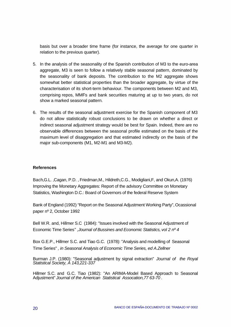
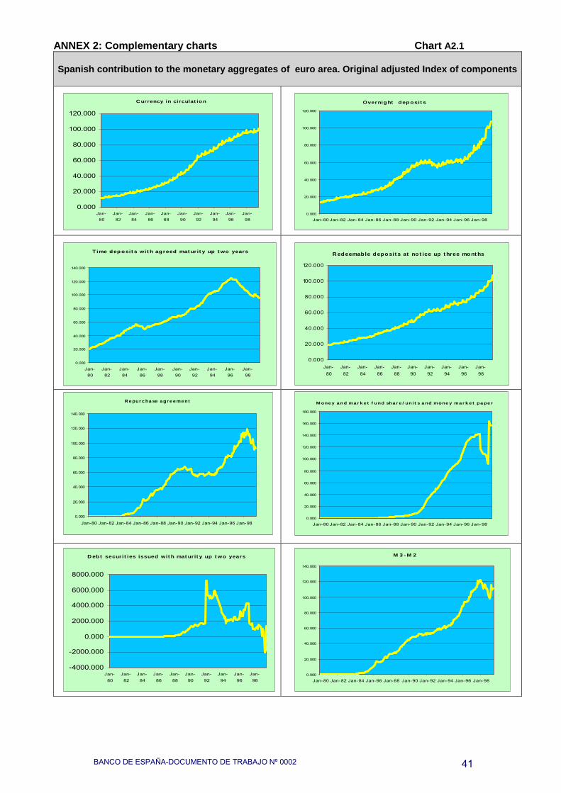
Table 1 presents the characterisation of the noise model and the differentoutliers identified in each of the components. In general terms, it is seen how, with theexception of the MMF and DEBSEC series, the models estimated show acceptablestatistical properties. In the case of the two components mentioned, the breaksobserved in the original series are indicative of the difficulty of modelling the behaviourof the series (see Chart A2.1 in Annex II).
4.1.2 Characterisation of the pattern
First, to obtain the best adjustment possible in the estimated single-equationmodels, allowing subsequently for the study of the profile of a series and optimalestimation of the unobservable components, it is necessary to isolate the possiblebreaks that might be identified and the profile of the series of aggregates andcomponents. The most significant interventions identified and estimated in relation tothe degree of incidence of some of the instruments considered in the light of theirinclusion or not in some of the aggregates are also presented in Table 1.
These breaks in the profiles of the series are principally associated withfinancial phenomena, such as the emergence of new instruments or changes inprevailing regulations that may prompt switching from one instrument to another, orchanges in the tax payment calendar that affect not only the trend pattern but also theseasonal behaviour of the series. By way of illustration, one of the latest effects toinvolve a break in the pattern of the Spanish monetary components in M3 was the taxreform that came into force in January 1999. However, the announcement of the entryinto force of these fiscal measures, which essentially entailed a relative improvement in
4 This effect is constructed on the basis of a matrix of six dummy variables (one for each day of the week, Sundayexcluded). The series have a 1 if the last day of the month falls on a trading day (Monday, Tuesday, Wednesday …Saturday) and 0 for the others. If the last day of the month is a Sunday, a -1 is introduced into each of the variables inthis position. In that way the "trading day" effect is cancelled out over the whole of the sample period considered. Onevariant that has not been considered in this study is that of considering the effect of public holidays that fall at the end ofthe month on appropriate weightings. We should like to acknowledge Björn Fisher for having provided these series anda description of them.
BANCO DE ESPAÑA-DOCUMENTO DE TRABAJO Nº 000210
the conditions for tax purposes of deposits as opposed to other financial assets suchas mutual funds, translated into a significant positive step effect on overnight deposits.This probably included the realisation of capital gains on mutual funds with a view toavoiding the withholding that began to be applied to these funds as from February1999. Likewise, deposits with a maturity of up to two years became, for much of 1999,recipients of money market mutual funds (FIAMMs and other fixed-income and equityfunds), contrary to what occurred in 1997. This all leads to the identification andestimation of a step effect in November 1998 in the series of deposits (OD, TD) and inthe aggregate M2. This effect has the opposite sign in the sub-component of M3-M2,and is neutralised in M3. However, the aggregate M1 does not reflect this effect.Likewise, the start of EMU has a transitory and marginal effect on the Spanishcomponent that is essentially reflected in a low-value impulse effect in the narroweraggregates.
With regard to the structure of the noise models, 8 of the 12 series analysedhave a stochastic seasonal structure reflected by means of a seasonal moving averageterm MA (12). A high value of the coefficient indicates that seasonality is lessstochastic and less mobile. Specifically, the components OD and RD are characterisedby their relatively non stochastic seasonal pattern. In the case of TD this pattern isvirtually deterministic. On the contrary, it can be seen how the series of cash held byother residents sectors (CUR) shows a very mobile seasonal pattern throughout thesample period, which is combined with an autoregressive structure that reflects anintra-annual cycle of quarterly periodicity. The seasonal pattern of the rest of thecomponents such as REPO, MMF and DEBSEC is much more blurred. Only theREPO series with the 12th-order seasonal autoregressive term shows apparently verymobile seasonality. It should be pointed out that one of the financial disturbances thathas most affected the historical trend of the monetary component in Spain was thepropagation of the 1985 Financial Assets Act, which granted favourable treatment in
relative terms to short-term government securities at the expense of bank products5.
This type of intense switching between components of the monetaryaggregates, generally associated with regulatory changes, has entailed significanttrend changes. These are reflected in the estimation of a high coefficient for theregular part of the stochastic structure, highlighting the presence of a relatively non-stochastic trend. This is the case of the components of MMF, REPO and DEBSEC, for
5 At that time the legislation appreciably affected not only trend changes but also the seasonal regularity of thenational monetary aggregates, insofar as the component chiefly affected by public portfolio switching was bankdeposits. Inasmuch as the distinguishing features of deposits and other types of instruments such as governmentsecurities became clearer, as did their role in the public's portfolios, the sizeable initial switching gradually diminished.This was reflected in the recovery by deposits of seasonal regularity and in the gradual appearance of a regularseasonal pattern for short-term public securities (which were included in the national aggregates in the past), and repos,associated with treasury management arrangements.
BANCO DE ESPAÑA- DOCUMENTO DE TRABAJO 0002 11
which periods of intense growth with subsequent and likewise intense declines arerecorded.
Logically, insofar as these processes are internalised in the broadest aggregate,the regular structure shows a more stochastic trend, as is the case of M3. In thenarrower aggregate, the only predominant pattern is a seasonal structure which, as canbe seen, highlights the weight in the Spanish component of M3 of deposits. The latter,along with cash, are the core of the seasonality of the monetary components.
4.2. Characterisation of the seasonal pattern
The following step after the estimation of the ARIMA models for each of theseries is the estimation of the seasonal component that will enable the correspondingseasonally adjusted series to be prepared.
As indicated in the foregoing section, the methodology was that of model-basedsignal extraction, using the SEATS application. The process of breaking down theseries into non-observable components (trend-cycle, seasonal and irregular) involvesan estimation of the theoretical model for each of them on the basis of the ARIMAmodel of the series observed. A comparative analysis of the results of the estimation ofthese components is made in this section. The focus is mainly on seasonality, havingregard to least estimation error criteria for the components, and a revision of theseasonal factors as new information becomes available.
It may be concluded from comparing these results that the seasonal patterns ofthe three monetary aggregates considered do not show marked differences. Evidently,all of them are dominated by the seasonal pattern of deposits, which are, along withcash, the core of seasonality, accounting for more than 75% of the Spanishcontribution to M3. This is why it may be ventured that this aggregate, both in terms ofits trend or seasonal adjustment, offers better qualities for short-term monitoring, sinceit may be deduced from the estimation of its non-observable components that the trendis smoother and estimated with less error. The M3 aggregate, however, showssomewhat worse qualities compared with M2. This is specifically apparent in theestimation of a greater contribution of the irregular component to the unpredictability ofthe series approximated by residual variance. This is mainly determined by the greatererraticism of the components encompassing M3-M2, the trend of which is marked bygreater volatility without such a marked trend or stochastical seasonal pattern.
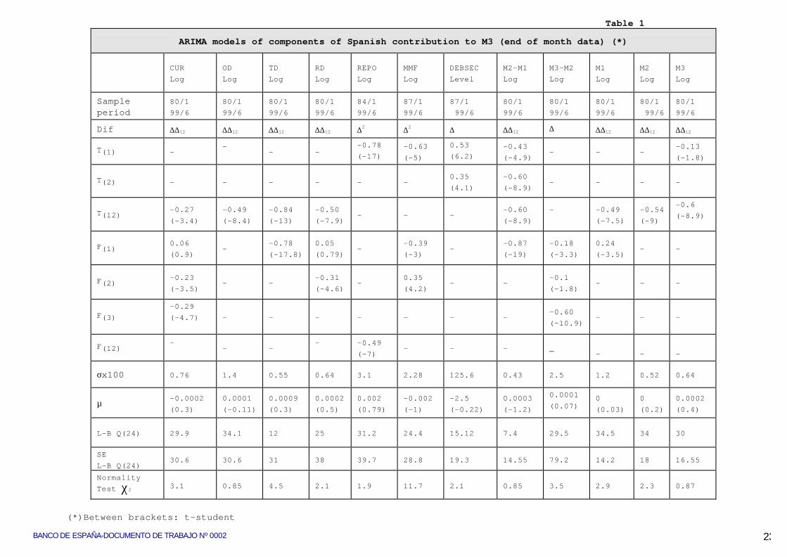
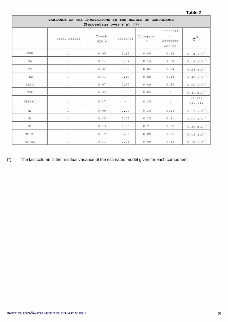
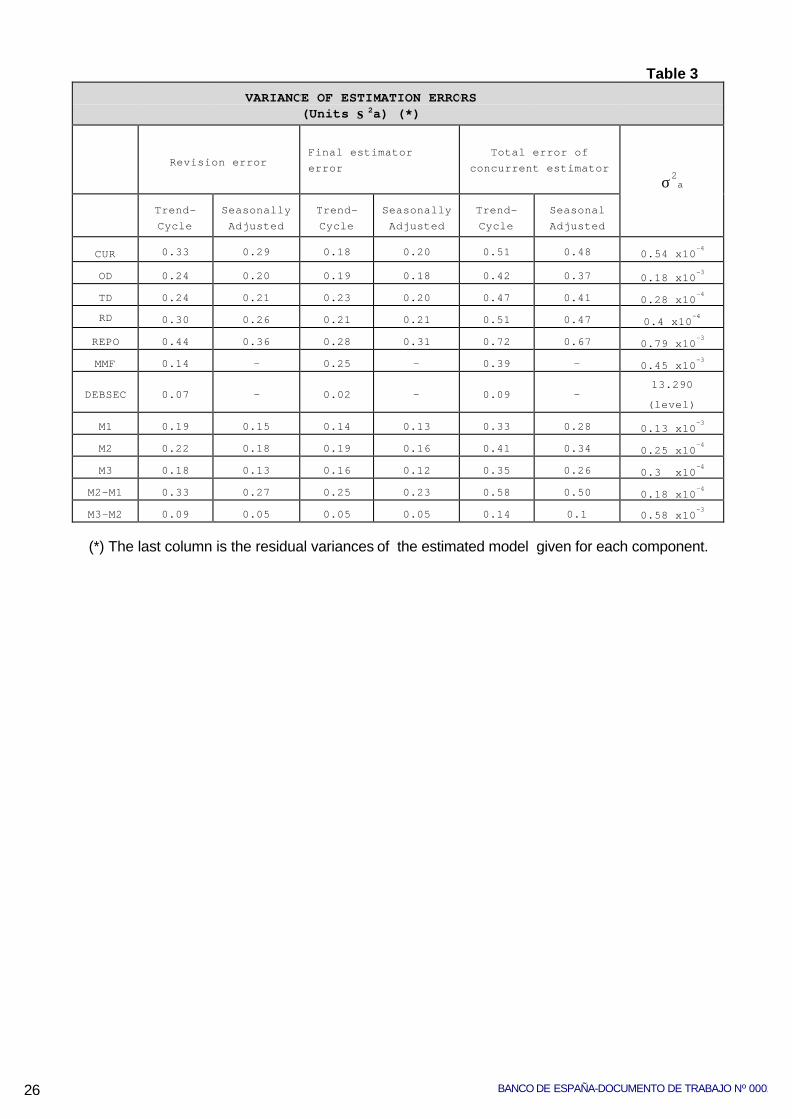
This type of conclusion can be obtained from analysis of the data in Tables 2and 3 in which the variance of the innovations and the variance of the estimation errorsof the non-observable components are respectively presented for each of the series

BANCO DE ESPAÑA-DOCUMENTO DE TRABAJO Nº 000212
analysed. Other comments that may be made on the various instruments andaggregates in the light of these tables might be the following:
• Currency displays a high contribution by seasonal components to the residual
variance of original series. Seasonally adjusted series significantly reduce theinnovation of original series. It is important to note that the innovation of the irregularcomponent is especially low.
• In the case of REPO, with the seasonal effect estimated by a AR(12) that canrepresent a highly stochastic seasonality, shows a high innovation of the seasonalcomponent too.
• The estimation of the Time deposits innovations shows a low contribution byseasonal components to the residual variance. It shows the higher volatility in thetrend-cycle component too. That implies a highly stochastic trend. This evidences thedifficulty of short-term monitoring of this component.
• Overnight Deposits presents a very high contribution of innovation by theirregular component linked to the seasonal one. This linked, to innovation in theseasonal component, suggests that the monitoring of this component would beimproved were trend component used, instead of seasonally adjusted series, althoughthe innovation of the trend component implies a very stochastic trend too.
• Looking at aggregates, in M1 the innovation of the seasonal effect of overnightdeposits predominates. The trend-cycle component shows a low innovation, probablydue to the offsetting of the effects of OD and CUR. That makes this signal more usefulthan the seasonal adjustment. Moreover the irregular component, also display a higherinnovation.
• The seasonal innovation of the rest of the deposits, and M1 is offset each other
M2-M1 the innovation of the seasonal component fades out, although this is not thecase for the innovation of the trend component that displays a high innovation.Moreover, the use of the seasonally adjusted series in M2, reduces the residualvariance of the original series by, approximately 40%.
• The rest of the components, between M2 and M3, are dominated by theinnovation of the trend-cycle and the very low innovation of the seasonal component.This innovation would correspond, mainly, to the seasonal innovation of REPO series.
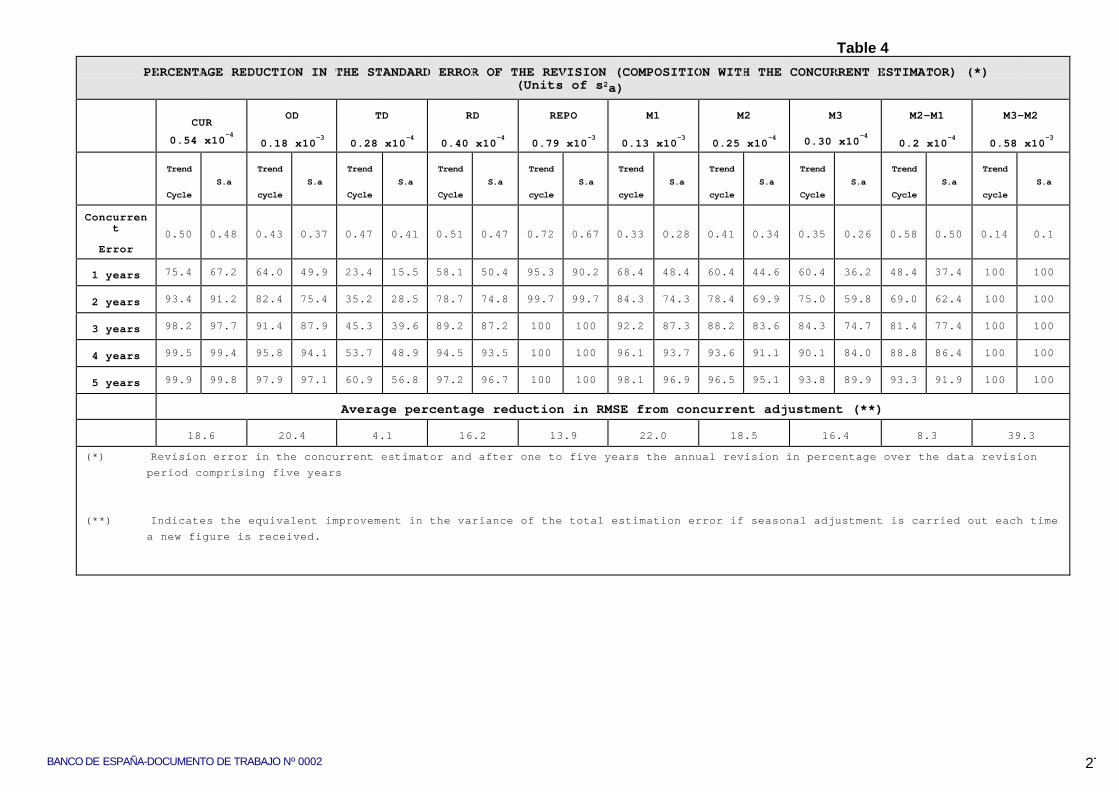
With respect to the estimator error of the non-observable components, it can beseen that, in general, the revision error (referring to the concurrent estimator, which in

BANCO DE ESPAÑA- DOCUMENTO DE TRABAJO 0002 13
turn is the estimator for month "t" when the latest data available are those of month "t")is around 50% of total error. This highlights that the series revision processsubstantially reduces revision error. Later, the degree to which the variance of theestimator is reduced is evaluated in the case of a concurrent adjustment in the variousseries.
It can further be seen in all the components that the trend-cycle estimator error,which is apparently a milder signal, is slightly higher than that of the adjusted series.The interpretation here could be that the use of a signal such as the trend-cycle signaldoes not generally mean an accurate estimation.
Considering the revision error of the contemporaneous estimator, Table 4shows how a revision process for both the trend-cycle estimator and for the seasonallyadjusted series is completed in virtually three years in the most liquid components(CUR and OD). This might advise the use of the concurrent estimation strategy forthese components, as well as for the aggregate M1, as the percentage of reduction ofthe residual variance infers. By contrary, in the case of term deposits, it is important tosee that this process of revision is much slower. This justifies the fact that, for M2 andM3, the advantage of using a concurrent adjustment procedure in terms of theimprovement in the quality of the adjustment is not as clear as in the case of M1. Thisis set against the disadvantages to be found in this type of seasonal adjustment owingto the problems of interpretation and comparison of the new information.
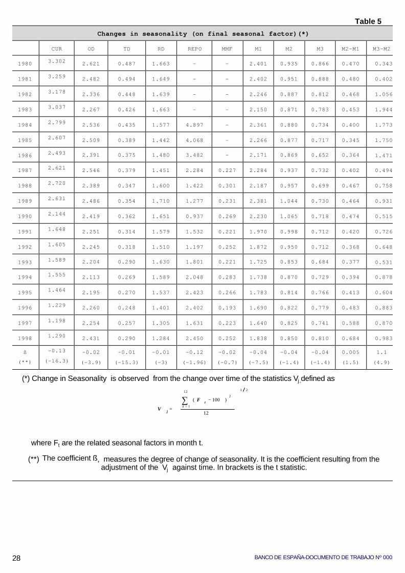
One of the most interesting results is the analysis of the degree of change inseasonality. Table 5 presents a statistic for the total (stochastic plus deterministic)seasonal factors for the different components and aggregates, which is obtained bycomputing the deviation of seasonal factors from 100 (which implies no seasonality).Thus, under the hypothesis of regularity of the seasonal component that would bederived from the low innovation estimated for this component, it might be affirmed thatthe higher values for Vj would indicate more marked seasonality (the seasonal factor isgreater the further the value is from 100). Conversely, much lower values for thisstatistic would infer the presence of less marked seasonality.
Hence, a horizontal reading enables the degree of seasonality of the differentaggregates and components to be compared. A vertical reading of the table shows thetrend of seasonality over time, insofar as the value Vj varies from one year to the next.Moreover, the adjustment of a simple regression against time of the related Vj
estimated for each aggregate gives a measure of the relevance of the trend of thisseasonality, as well as the direction of this trend.
BANCO DE ESPAÑA-DOCUMENTO DE TRABAJO Nº 000214
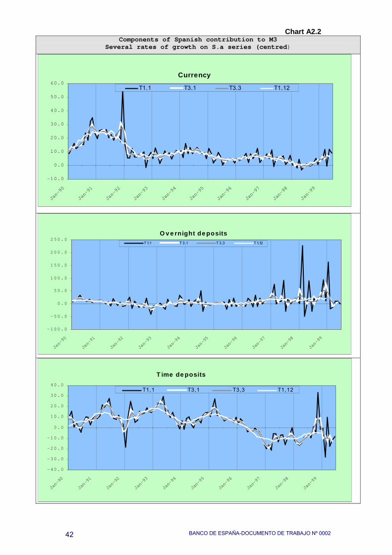
One of the most relevant points in this characterisation is the change ofseasonality of currency since 1980. The spread of use of ATM (Automated tellermachines) and plastic money, has made the seasonality less marked and the loss of aseasonal pattern has been very significant in the last twenty years. By contrary, ODmaintains the seasonal pattern associated with the payment of salaries, interest ratepayments, and taxation, i.e. this series maintains a very close link to the annual patternof the public´s income/spending. The same is the case with RD. Other componentsmore associated with the saving concept, depending more on changes in interest ratesand other aspects with lesser marked seasonality, generally, less marked and arerelatively stable over time.
Apparently, the seasonality of REPO series is very marked. This is odd,because these financial assets have traditionally substituted TD and the seasonality ofTD is more related to the role of this component in the financial innovation process,until the finalisation of the fiscal harmonisation process. 1984 saw the first public debtrepos, and these were very attractive in relation to TD or other deposits. In 1985 therewas a law of fiscal reform of financial assets, and in 1987 the Treasury bill issuesbegan. Comparing the trend and degree of seasonality of the various aggregates, themost marked seasonality is seen to be that of M1. This pattern has also changedconsiderably, becoming progressively blurred over the years, while in the case of theother two aggregates, seasonality that is not so marked and changes less hasprevailed. In this respect, it is important to analyse the degree of internalisation ofseasonality between components. M2 and M3 reflect the neutralisation in theseasonality between deposits and repos and MMFs. Consequently, M2 and M3 remainvery stable over time in the seasonal pattern, which is associated with the integration ofcomponents with a relatively different seasonal pattern offsetting one another.
4.2.1 Suitable filters for evaluating growth rates
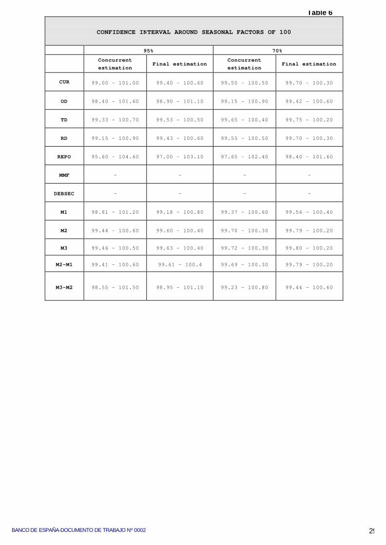
Another notable features of the methodology used is the ability to obtainconfidence intervals for the growth rates estimated drawing on the seasonally adjustedseries, as well as for the seasonal factors. This inference analysis reflects to someextent the results relative to estimation errors, the revision of non-observablecomponents, changes in seasonality, etc, discussed previously.
The confidence intervals estimated for the final factors presented in Table 6indicate the width that this interval represents in respect of the level of the series.These intervals highlight, in the case of the three aggregates considered, that M3 hasthe least width in its confidence interval, from 1% in terms of the contemporaneousestimator to 95% confidence of the estimation, declining to 0.8% of the level of theseries in terms of the final estimator. For its part, M2 has a very similar width to that of
BANCO DE ESPAÑA- DOCUMENTO DE TRABAJO 0002 15
M3. Without being particularly big, these intervals give some idea of the degree ofcaution with which the seasonally adjusted data of the monetary aggregates must behandled. Nonetheless, the width difference between the contemporaneous and finalestimators also highlights that the information revision process is not particularlyrelevant in determining the goodness of fit in the estimation of seasonal factors in thecase of an annual projection strategy (and in the absence of additional revisions of theoriginal series). However, in the case of M1 the difference in the estimated intervalwidths for the factors relative to the contemporaneous or the final estimators broadensto almost 0.7% of the level of the series. It is seen how this estimated interval forfactors duplicates in relation to that of the aggregates M2 or M3.
In respect of some of the components, it might be pointed out that the seasonalfactors of term deposits up to a maturity of two years are those which show least width,of around 1%. The estimated width in the case of REPOS gives some idea of the scantquality of the estimation of seasonal factors and the caution required in interpreting theseasonally adjusted components. Yet insofar as monitoring and the growth references(or targets) are set in terms of rates, it is worth analysing the effect of measurementerrors on these growth rates.
In this respect, Table 7 offers the different types of rates traditionally used in theBanco de España in monitoring the monetary aggregates or other financialmagnitudes. In order to make annual growth references comparable, the shortest-dated rates, which measure month-on-month or quarter-on-quarter changes, areannualised. It is known that such annualisation implicitly entails a prediction in the
sense that the latest estimated change holds constant for the rest of the year6 7.
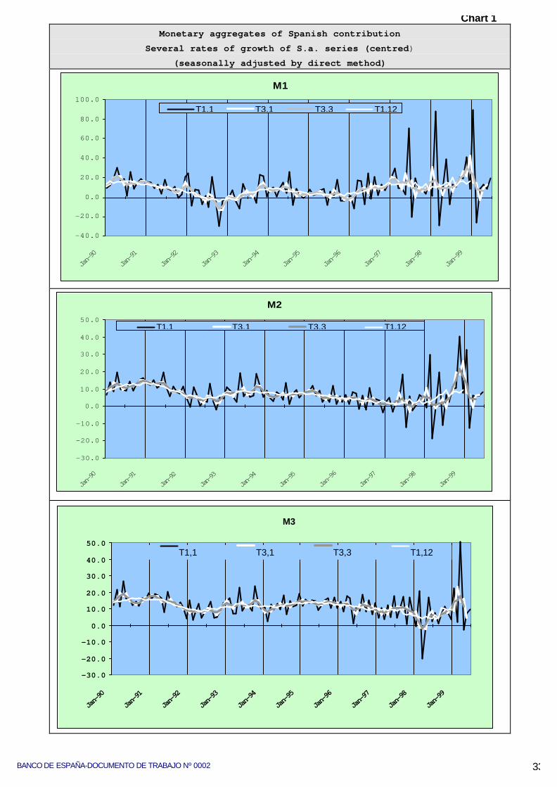
The problem posed by a rate as short as that of a month-on-month growth rate(whether annualised or not) is the fact that, frequently, the month-to-monthinterpretation is especially difficult as it is confined to such a short space of time.Occasionally, this may be determined by a "discrete" disturbance that may affect aspecific month, or by the very provisionality of the latest data with which this type ofrate is calculated. This is why the Banco de España has also used other short rates inwhich an interval of several months is averaged. That gives a less erratic pattern asregards the trend of the aggregate. Chart 1 shows the monetary aggregates usingseveral growth rates for the series, which have undergone seasonal adjustment by thedirect method. It can be seen how rates such as T1
3 (T13 and T3
1 are virtually
6 In the use of annualised rates, it is also assumed that, in respect of annual rates, variance is not homogeneous.
7 Another aspect that should be taken into account in the comparison between annual rates and month-on-monthrates (whether annualised or not) is the centring of the former in order to set them in phase with what we call "basicgrowth" in Table 7. No considerations are made in this section of the advisability or not of centring rates.

BANCO DE ESPAÑA-DOCUMENTO DE TRABAJO Nº 000216
equivalent) or T33 are alternative rates which, if they are centred, show an identical
profile to the foregoing month-on-month rate, only smoother.
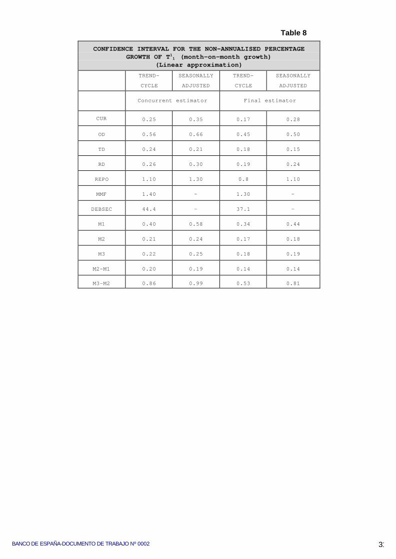
Turning to the analysis and interpretation of the confidence intervals estimatedfor these rates, it should be pointed out that the size of the errors is the barrier to themeasurement of the monthly growth of the seasonally adjusted series and the trend.Logically, the greater variability of the shortest rates becomes particularly patent in thegreater width estimated for the confidence interval. This underscores what waspreviously said regarding the caution required for interpreting the results in terms of arate as short as, for example, T1
1. In this respect, Table 8 presents the confidenceinterval for month-on-month non-annualised growth.
The interval band for trend-cycle is for all components less than s.a. series,although the estimator error for trend is generally higher. The interval around T1
1 of thetrend is lower, due to the presence of greater autocorrelation in its errors series. Ingeneral, there are few differences between the intervals of trend and s.a. There is onlya more relevant difference in the case of the “core” of liquidity. Indeed, it is possible tosee how in the components and aggregates with more marked seasonality and higherinnovation in seasonal component, there is a greater difference between trend and s.a(CUR,OD and M1). For these components and M1, a signal such as trend would bemore recommendable in short-term monitoring.
On the contrary, for the TD series, the interval for trend is slightly higher. It is inconsonance with that shown before of an estimation of a smooth and less markedseasonality.
In the case of M3, the interval using the concurrent estimator is 0.25 (3percentage points in annualised terms). In terms of final estimators after revision it isreduced to 2.3%. This interval for the Spanish M3 seems a little bit smaller thanestimated for our old ALP and ALPF.
The potential use of this confidence interval would be as follows:
If, for example, +/- 3 % was the interval estimated for euro-area M3 aggregateand the growth in August 99 was 0.0, the true value could be between –3% or +3%. Inthis case it is significantly below 4.5%. On the contrary, in September 99 it was 0.6 (7.2points annualised ), when the lower significance band is 4.2%; this implies that 4.5%is in the lower limit So, if there were a persistent month-on-month growth of around6%, it could be compatible with the reference, depending on the month-on monthconfidence band

BANCO DE ESPAÑA- DOCUMENTO DE TRABAJO 0002 17
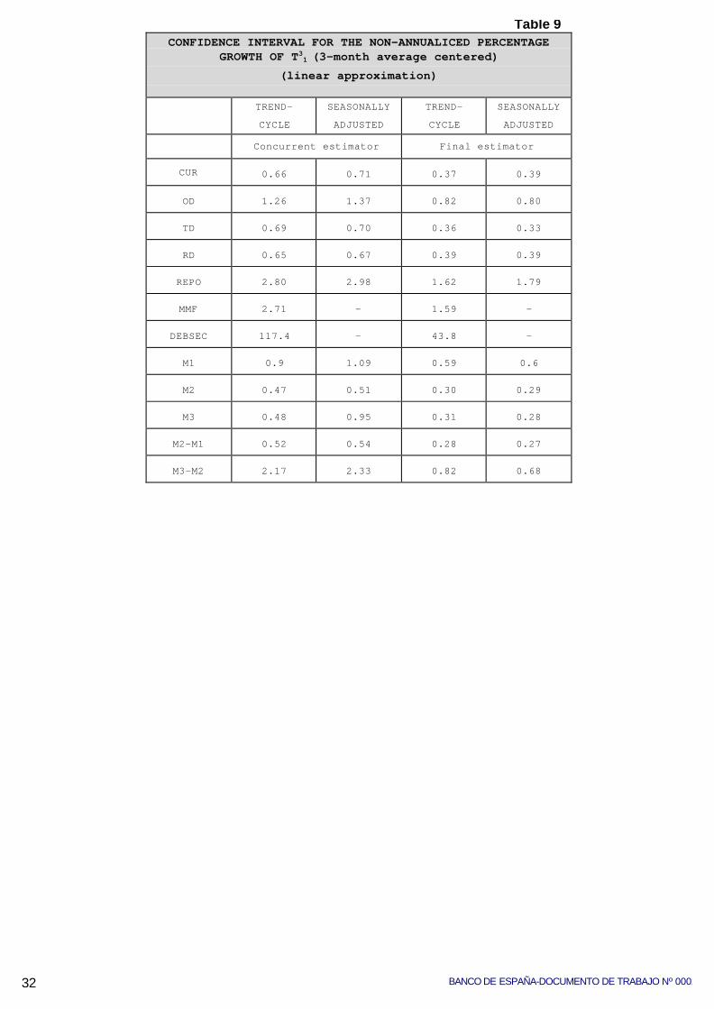
Obviously, in terms of a smoother rate of growth such as a 3-month movingaverage - T3
1 -, the confidence interval is lower and, consequently, it is possible tomonitor the reference more accurately (Table 9).
In conclusion, if the annual growth reference were in terms of a T312, the short
term month-on-month, monitoring could be more appropriate using the T31 or using an
smoother rates of growth like T33. Concretely, for the Spanish contribution to M3, the
confidence band of the final estimator error, using the T31 s.a. series, falls by around
1.2 points, practically reducing the uncertainty by 50% , in comparison with the T11.
4.3. Evaluation of direct versus indirect adjustment
One of the methodological aspects which most usually concerns users ofseasonal adjustment techniques and analysts of this information is the choice of theaggregation strategy to be followed to obtain seasonal adjustment, mainly in the caseof the main variables, such as the monetary and credit magnitudes, or of othereconomic indicators such as the consumer price index.
Evaluation of the better quality that a -direct or indirect- seasonal adjustment ofan aggregate can offer will depend on the features of each particular case. Specificrules cannot be set since the best strategy depends on many factors: e.g. the intensityof potential switching processes involving components, the seasonal pattern that suchcomponents may follow, and, in this respect, the greater or lesser impact on thisseasonal pattern of the switching processes. Naturally, there are other more subjectivefactors such as the use that is to be made of the seasonally adjusted information, theimportance attached to the principle of additivity, etc.
One of the initial aspects to be analysed when the selection of the seasonaladjustment strategy is tackled is the degree of correlation between the components ofan aggregate. A simple graphic inspection of the original series of these componentscan already give an idea of this potential correlation. In the case of Spain, as in that ofother countries, an intense switching process is observed; this involves negativecorrelation between term deposits and repos, firstly, and mutual funds, subsequently.(See once again chart A2.1 and A2.2 in the annex II).
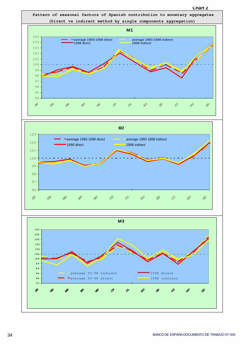
Another means of evaluating the quality of direct versus indirect seasonaladjustment is to compare the differences between the seasonal pattern obtained fromthe factors estimated by the direct method with that obtained by the indirect procedure.Specifically, the better quality of the adjustment can be assessed by having regard tothe criterion of minimum variance of the stochastic factor. However, an analysis hasbeen conducted here in respect of the lesser variability of the final factors.
BANCO DE ESPAÑA-DOCUMENTO DE TRABAJO Nº 000218
Chart 2 depicts the seasonal profile estimated for the aggregates M1 to M3under both approaches. In the case of M2, it is first seen how this seasonal profile hasheld very stable in recent years (average of 93-98) in relation to that estimated for theyear 98. The stability is highlighted both in the direct and indirect approach. Bothprofiles are virtually identical, which underscores the fact that there are nosuperimposed seasonal effects between components and aggregates, a relativelymarked profile being sustained in each of the components. This similarity in seasonalprofiles is evidently determined by the seasonality of deposits, in response to a moremarked seasonal pattern and to the very weight of deposits in the composition of thenarrower aggregates.
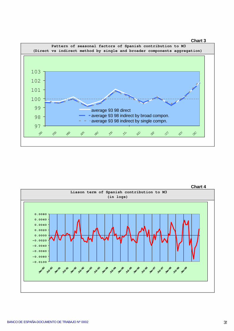
The seasonal profile of M3 does not show any great differences either betweenthe indirect and direct approach on average between the years 93-98. In terms ofvariability, the indirect approach is only marginally somewhat more volatile. Thisgreater variability is more patent in a comparison of the profiles estimated for the year1998. In this respect, despite the fact that the component of M3-M2 is that whichpresents a more variable seasonal pattern, its incidence in the seasonality of theaggregate obtained by the indirect method is not relevant. On one hand, in the total ofthe aggregate this sub-component does not reach 23%, of which amount banksecurities and MMFs (10% of M3, approximately) show no clear evidence of thepresence of seasonality. Indeed, an additional exercise consisting of the considerationof these two components has no incidence either on the estimation of the implicitfactors obtained by the indirect adjustment or on the estimation of the related shortrates of the seasonally adjusted series. In this context, the indirect approach by sub-component (M1, M2-M1 and M3-M2) in the Spanish case gives virtually identicalresults to the indirect adjustment process at the maximum level of dissagregation, asis are observed in Chart 3.
A complementary exercise to compare the degree of discrepancy between bothmethods is to analyse what we have called the liaison term, which is shown in Chart 4.This is the difference between the aggregate seasonal adjustment and the seasonaladjustment obtained by aggregation of the seasonally adjusted components. Twopoints may be made here. First, the scale of the discrepancy in absolute terms or as alog (percentage of discrepancy in relation to the level of the series). And second,potential residual seasonality, i.e. the seasonality not reflected by the indirect method,and which would implicitly be internalised in the direct adjustment. Evidence of a liaisonterm with a defined seasonal profile and one of some scale would show that theseasonality of the aggregate would be better reflected having regard to a directseasonal adjustment criterion.

BANCO DE ESPAÑA- DOCUMENTO DE TRABAJO 0002 19
In our specific case, the scale of the liaison term can be seen to relatively small,oscillating between 0.8% and -0.9% of the level of the series. Moreover, although aslight seasonal pattern is perceptible in the behaviour of the liaison term around theperiod 93 to 95, this becomes blurred at the end of the sample while the scale of theterm increases.
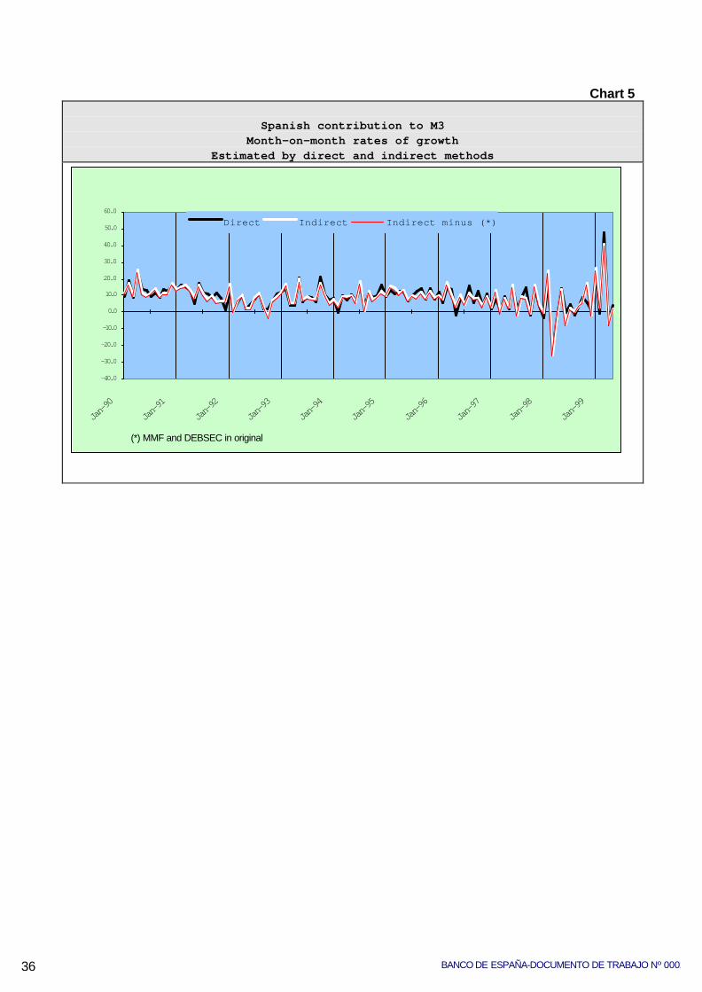
Thus, having regard both to the analysis of the variability of the seasonalprofiles estimated for both strategies and to the evidence that may be derived from theliaison term, on the information analysed there is no robust statistical evidencesupporting either seasonal adjustment strategy in the case of the Spanish component.Indeed, in terms of the variability of short growth rates, the estimated profiles are verysimilar, although in the final years of the sample (1997 to 1999) the volatility of therates estimated for the direct adjustment is slightly less (see Chart 5).
5. CONCLUSIONS
1. In the regular seasonal adjustment exercises for its main economic indicators, theBanco de España has traditionally used the ARIMA model-based signal extractionmethod and, specifically, the TRAMO/SEATS procedure.
2. The reason for using this methodology and procedure lies mainly in the fact thatthis method offers information on the properties of the estimators used and of theestimation errors. Specifically, the methodology makes it possible to performinference analysis and a diagnosis of the non-observable components. In thisrespect, the TRAMO/SEATS application provides a robust statistical informationinfrastructure to conduct an exercise involving the decomposition of the time seriesinto its non-observable components.
3. The monetary and credit aggregates were subject to regular seasonal adjustmentat the Banco de España. This seasonal adjustment exercise was conductedannually and its results (projection and revision of factors) and othermethodological factors were published in the Banco de España Boletín Económico.
4. The change in the monetary policy implementation strategy over the course of thenineties entailed a sizeable loss in the significance of the very short-termmonitoring of the monetary aggregates, and the consequent relativisation of therole of the seasonally adjusted series of the monetary aggregates. In any event, theofficial seasonal adjustment of the monetary aggregates has been performeduninterruptedly through to 1999, insofar as the seasonally adjusted seriescontinued to provide for short-term monitoring not so much on a month-to-month
BANCO DE ESPAÑA-DOCUMENTO DE TRABAJO Nº 000220
basis but over a broader time frame (for instance, the average for one quarter inrelation to the previous quarter).
5. In the analysis of the seasonality of the Spanish contribution of M3 to the euro-areaaggregate, M3 is seen to follow a relatively stable seasonal pattern, dominated bythe seasonality of bank deposits. The contribution to the M2 aggregate showssomewhat better statistical properties than the broader aggregate, by virtue of thecharacterisation of its short-term behaviour. The components between M2 and M3,comprising repos, MMFs and bank securities maturing at up to two years, do notshow a marked seasonal pattern.
6. The results of the seasonal adjustment exercise for the Spanish component of M3do not allow statistically robust conclusions to be drawn on whether a direct orindirect seasonal adjustment strategy would be best for Spain. Indeed, there are noobservable differences between the seasonal profile estimated on the basis of themaximum level of disaggregation and that estimated indirectly on the basis of themajor sub-components (M1, M2-M1 and M3-M2).
References
Bach,G.L. ,Cagan, P.D. , Friedman,M., Hildreth,C.G., Modigliani,F, and Okun,A. (1976)Improving the Monetary Aggregates: Report of the advisory Committee on MonetaryStatistics, Washington D.C.: Board of Governors of the federal Reserve System
Bank of England (1992) “Report on the Seasonal Adjustment Working Party”, Ocassionalpaper nº 2, October 1992
Bell W.R. and, Hillmer S.C (1984): "Issues involved with the Seasonal Adjustment ofEconomic Time Series” ,Journal of Bussines and Economic Statistics, vol 2 nº 4
Box G.E.P., Hillmer S.C. and Tiao G.C. (1978): "Analysis and modelling of Seasonal
Time Series" , in Seasonal Analysis of Economic Time Series, ed A.Zellner
Burman J.P. (1980): "Seasonal adjustment by signal extraction" Journal of the RoyalStatistical Society, A 143,221-337
Hillmer S.C. and G.C. Tiao (1982): "An ARIMA-Model Based Approach to SeasonalAdjustment” Journal of the American Statistical Assocation,77 63-70 .

BANCO DE ESPAÑA- DOCUMENTO DE TRABAJO 0002 21
Gómez, V. and Maravall, A. (1996), “Programs TRAMO and SEATS”, in Banco deEspaña, working paper 9628
Gómez, V. and Maravall, A. (1998), “Guide for using the programs TRAMO and SEATS”,in Banco de España, working paper nº 9805
Gómez, V. and Maravall, A. (1998), “Automatic modeling methods for univariate series”, inBanco de España, working paper nº 9808. Forthcoming, in A Course in Time Series (eds.D.Peña, G.C. Tiao, and R.S. Tsay). N.Y. I.Wiley and sons
Gomez, V. and Maravall, A. (1998), “Seasonal adjustment and signal extraction ineconomic time series” working paper nº 9809. Forthcoming, in A Course in Time Series(eds. D.Peña, G.C. Tiao, and R.S. Tsay). N.Y. I.Wiley and sons
Maravall, A. (1984): “On issues involved with the seasonal adjustment of time series”,Banco de España ,working paper nº 8408. Also in Journal of Business and EconomicStatistics , 2, 1984
Maravall, A. (1987): “The Use of ARIMA Models in Unobserved Components Estimation:an application to spanish monetary control”, Banco de España , working paper nº 8701.Also in Dynamic Econometric Modelling, Prceedings of the third International Symposiumin Economic Theory and Econometrics, Austin (Cambridge):Cambridge UniversityPress,1998
Maravall, A. (1997): “Two discussions on new seasonal adjustment methods”, Banco deEspaña , working paper 9704. Also in Journal of Business and Economic Statistics , 2,1998
Moore, G.H., Box,G.E.P., Kaitz,H.B., Stephenson,J.A. and Zellner,A. (1981), SeasonalAdjustment of the Monetary Aggregates: Report of the Committee of Experts on SeasonalAdjustment Techniques, Washington D.C.: Board of Governors of the Federal ReserveSystem

BANCO DE ESPAÑA-DOCUMENTO DE TRABAJO Nº 000222
TTAABBLLEESS AANNDD CCHHAARRTTSS
BANCO DE ESPAÑA-DOCUMENTO DE TRABAJO Nº 0002 23
Table 1
ARIMA models of components of Spanish contribution to M3 (end of month data) (*)
CURLog
ODLog
TDLog
RDLog
REPOLog
MMFLog
DEBSECLevel
M2-M1Log
M3-M2Log
M1Log
M2Log
M3Log
Sampleperiod
80/1 99/6
80/1 99/6
80/1 99/6
80/1 99/6
84/1 99/6
87/1 99/6
87/1 99/6
80/1 99/6
80/1 99/6
80/1 99/6
80/1 99/6
80/1 99/6
Dif ∆∆12 ∆∆12 ∆∆12 ∆∆12 ∆2 ∆2 ∆ ∆∆12 ∆ ∆∆12 ∆∆12 ∆∆12
T(1) --
- --0.78(-17)
-0.63(-5)
0.53(6.2)
-0.43(-4.9)
- - --0.13(-1.8)
T(2) - - - - - -0.35(4.1)
-0.60(-8.9)
- - - -
T(12)-0.27(-3.4)
-0.49(-8.4)
-0.84(-13)
-0.50(-7.9)
- - --0.60(-8.9)
- -0.49(-7.5)
-0.54(-9)
-0.6(-8.9)
F(1)0.06(0.9)
--0.78(-17.8)
0.05(0.79)
--0.39(-3)
--0.87(-19)
-0.18(-3.3)
0.24(-3.5)
- -
F(2)-0.23(-3.5)
- --0.31(-4.6)
-0.35(4.2)
- --0.1(-1.8)
- - -
F(3)-0.29(-4.7) - - - - - - -
-0.60(-10.9)
- - -
F(12)-
- -- -0.49
(-7)- - - _
- - -
σx100 0.76 1.4 0.55 0.64 3.1 2.28 125.6 0.43 2.5 1.2 0.52 0.64
µ-0.0002(0.3)
0.0001(-0.11)
0.0009(0.3)
0.0002(0.5)
0.002(0.79)
-0.002(-1)
-2.5(-0.22)
0.0003(-1.2)
0.0001(0.07)
0(0.03)
0(0.2)
0.0002(0.4)
L-B Q(24) 29.9 34.1 12 25 31.2 24.4 15.12 7.4 29.5 34.5 34 30
SEL-B Q(24)
30.6 30.6 31 38 39.7 28.8 19.3 14.55 79.2 14.2 18 16.55
NormalityTest χ2 3.1 0.85 4.5 2.1 1.9 11.7 2.1 0.85 3.5 2.9 2.3 0.87
(*)Between brackets: t-student

BANCO DE ESPAÑA-DOCUMENTO DE TRABAJO Nº 000224
Table 1 (cont.)AUTOMATIC OUTLIERS IDENTIFICATION WITH TRAMO
CUR OD TD RD REPO MMF DEBSEC M2-M1 M3-M2 M1 M2 M3
Dec-80 TC
Dec-81 TC
Oct-82 LS
Dec-82 LS
Mar-83 TC LS
May-83 TC
Oct-83 AO
Jan-84 LS
Jun-84 LS
Aug-84 AO
Sep-84 LS
Oct-84 LS
Mar-85 AO AO
May-85 AO TC TC TC
Aug-85 TC
Oct-85 LS
Dec-85 LS
Apr-86 TC LS
May-86 TC TC
Jul-86 LS LS
Aug-86 LS LS
Apr-87 AO
May-87 TC
Jun-87 TC LS
Nov-87 AO
Mar-88
Jul-88 LS LS LS
Mar-89 TC AO
Jul-89 AO TC TC AO TC
Mar-90 AO
Abr-90 LS
Dec-91 TC AO
Jan-92 TC LS LS
Mar-92 LS
Jun-92 AO
Oct-92 LS LS
Feb-93 AO
Apr-93 AO
Dec-93 LS
Jun-94 TC
Jul-94 AO
Jun-96 TC
Sep-96 LS
Nov-96 AO
Dec-96 LS
Feb-97 LS
May-97 LS
Jun-97 TC AO AO
Sep-97 AO
Feb-98 AO AO AO
Mar-98 AO LS LS
May-98 AO AO
Jun-98 AO TC
Nov-98 LS LS LS
Nov-98 LS
Dec-98 AO
Jan-99 TC AO AO AO
Feb-99 AO TC TC
Mar-99 LS LS TC
Apr-99 LS
Jun-99 AO
Total
number5 12 7 1 6 5 15 6 16 5 11 3
BANCO DE ESPAÑA-DOCUMENTO DE TRABAJO Nº 0002 25
Table 2
VARIANCE OF THE INNOVATIONS IN THE MODELS OF COMPONENTS(Percentage over σ2a) (*)
Total SeriesTrend-cycle
SeasonalIrregula
r
Seasonally
Adjusted
Series
σ2a
CUR 1 0.06 0.19 0.05 0.38 0.54 x10⁻⁴
OD 1 0.14 0.09 0.14 0.57 0.18 x10⁻³
TD 1 0.32 0.02 0.06 0.84 0.28 x10⁻⁴
RD 1 0.11 0.14 0.08 0.44 0.40 x10⁻⁴
REPO 1 0.07 0.27 0.09 0.39 0.80 x10⁻³
MMF 1 0.33 - 0.05 1 0.45 x10⁻³
DEBSEC 1 0.47 - 0.10 113.290(level)
M1 1 0.09 0.07 0.16 0.58 0.13 x10⁻³
M2 1 0.15 0.07 0.15 0.61 0.25 x10⁻⁴
M3 1 0.13 0.05 0.21 0.68 0.30 x10⁻⁴
M2-M1 1 0.19 0.05 0.09 0.65 0.18 x10⁻⁴
M3-M2 1 0.11 0.06 0.09 0.53 0.58 x10⁻³
(*) The last column is the residual variance of the estimated model given for each component
BANCO DE ESPAÑA-DOCUMENTO DE TRABAJO Nº 000226
Table 3
VARIANCE OF ESTIMATION ERRORS(Units σ2a) (*)
Revision errorFinal estimatorerror
Total error ofconcurrent estimator
Trend-Cycle
SeasonallyAdjusted
Trend-Cycle
SeasonallyAdjusted
Trend-Cycle
SeasonalAdjusted
σ2a
CUR 0.33 0.29 0.18 0.20 0.51 0.48 0.54 x10⁻⁴
OD 0.24 0.20 0.19 0.18 0.42 0.37 0.18 x10⁻³
TD 0.24 0.21 0.23 0.20 0.47 0.41 0.28 x10⁻⁴
RD 0.30 0.26 0.21 0.21 0.51 0.47 0.4 x10⁻⁴
REPO 0.44 0.36 0.28 0.31 0.72 0.67 0.79 x10⁻³
MMF 0.14 - 0.25 - 0.39 - 0.45 x10⁻³
DEBSEC 0.07 - 0.02 - 0.09 -13.290
(level)
M1 0.19 0.15 0.14 0.13 0.33 0.28 0.13 x10⁻³
M2 0.22 0.18 0.19 0.16 0.41 0.34 0.25 x10⁻⁴
M3 0.18 0.13 0.16 0.12 0.35 0.26 0.3 x10⁻⁴
M2-M1 0.33 0.27 0.25 0.23 0.58 0.50 0.18 x10⁻⁴
M3-M2 0.09 0.05 0.05 0.05 0.14 0.1 0.58 x10⁻³
(*) The last column is the residual variances of the estimated model given for each component.
BANCO DE ESPAÑA-DOCUMENTO DE TRABAJO Nº 0002 27
Table 4
PERCENTAGE REDUCTION IN THE STANDARD ERROR OF THE REVISION (COMPOSITION WITH THE CONCURRENT ESTIMATOR) (*) (Units of s2a)
CUR
0.54 x10⁻⁴
OD
0.18 x10⁻³
TD
0.28 x10⁻⁴
RD
0.40 x10⁻⁴
REPO
0.79 x10⁻³
M1
0.13 x10⁻³
M2
0.25 x10⁻⁴
M3
0.30 x10⁻⁴
M2-M1
0.2 x10⁻⁴
M3-M2
0.58 x10⁻³
Trend
CycleS.a
Trend
cycleS.a
Trend
CycleS.a
Trend
CycleS.a
Trend
cycleS.a
Trend
cycleS.a
Trend
cycleS.a
Trend
CycleS.a
Trend
CycleS.a
Trend
cycleS.a
Concurrent
Error0.50 0.48 0.43 0.37 0.47 0.41 0.51 0.47 0.72 0.67 0.33 0.28 0.41 0.34 0.35 0.26 0.58 0.50 0.14 0.1
1 years 75.4 67.2 64.0 49.9 23.4 15.5 58.1 50.4 95.3 90.2 68.4 48.4 60.4 44.6 60.4 36.2 48.4 37.4 100 100
2 years 93.4 91.2 82.4 75.4 35.2 28.5 78.7 74.8 99.7 99.7 84.3 74.3 78.4 69.9 75.0 59.8 69.0 62.4 100 100
3 years 98.2 97.7 91.4 87.9 45.3 39.6 89.2 87.2 100 100 92.2 87.3 88.2 83.6 84.3 74.7 81.4 77.4 100 100
4 years 99.5 99.4 95.8 94.1 53.7 48.9 94.5 93.5 100 100 96.1 93.7 93.6 91.1 90.1 84.0 88.8 86.4 100 100
5 years 99.9 99.8 97.9 97.1 60.9 56.8 97.2 96.7 100 100 98.1 96.9 96.5 95.1 93.8 89.9 93.3 91.9 100 100
Average percentage reduction in RMSE from concurrent adjustment (**)
18.6 20.4 4.1 16.2 13.9 22.0 18.5 16.4 8.3 39.3
(*) Revision error in the concurrent estimator and after one to five years the annual revision in percentage over the data revisionperiod comprising five years
(**) Indicates the equivalent improvement in the variance of the total estimation error if seasonal adjustment is carried out each timea new figure is received.
BANCO DE ESPAÑA-DOCUMENTO DE TRABAJO Nº 000228
Table 5
Changes in seasonality (on final seasonal factor)(*)
CUR OD TD RD REPO MMF M1 M2 M3 M2-M1 M3-M2
1980 3.302 2.621 0.487 1.663 - - 2.401 0.935 0.866 0.470 0.343
1981 3.259 2.482 0.494 1.649 - - 2.402 0.951 0.888 0.480 0.402
1982 3.178 2.336 0.448 1.639 - - 2.246 0.887 0.812 0.468 1.056
1983 3.037 2.267 0.426 1.663 - - 2.150 0.871 0.783 0.453 1.944
1984 2.799 2.536 0.435 1.577 4.897 - 2.361 0.880 0.734 0.400 1.773
1985 2.607 2.509 0.389 1.442 4.068 - 2.266 0.877 0.717 0.345 1.750
1986 2.493 2.391 0.375 1.480 3.482 - 2.171 0.869 0.652 0.364 1.471
1987 2.621 2.546 0.379 1.451 2.284 0.227 2.284 0.937 0.732 0.402 0.494
1988 2.720 2.389 0.347 1.600 1.422 0.301 2.187 0.957 0.699 0.467 0.758
1989 2.631 2.486 0.354 1.710 1.277 0.231 2.381 1.044 0.730 0.464 0.931
1990 2.144 2.419 0.362 1.651 0.937 0.269 2.230 1.065 0.718 0.474 0.515
1991 1.648 2.251 0.314 1.579 1.532 0.221 1.970 0.998 0.712 0.420 0.726
1992 1.605 2.245 0.318 1.510 1.197 0.252 1.872 0.950 0.712 0.368 0.648
1993 1.589 2.204 0.290 1.630 1.801 0.221 1.725 0.853 0.684 0.377 0.531
1994 1.555 2.113 0.269 1.589 2.048 0.283 1.738 0.870 0.729 0.394 0.878
1995 1.464 2.195 0.270 1.537 2.423 0.266 1.783 0.814 0.766 0.413 0.604
1996 1.229 2.260 0.248 1.401 2.402 0.193 1.690 0.822 0.779 0.483 0.883
1997 1.198 2.254 0.257 1.305 1.631 0.223 1.640 0.825 0.741 0.588 0.870
1998 1.290 2.431 0.290 1.284 2.450 0.252 1.838 0.850 0.810 0.684 0.983
ß
(**)
-0.13
(-16.3)-0.02
(-3.9)
-0.01
(-15.3)
-0.01
(-3)
-0.12
(-1.96)
-0.02
(-0.7)
-0.04
(-7.5)
-0.04
(-1.4)
-0.04
(-1.4)
0.005
(1.5)
1.1
(4.9)
(*) Change in Seasonality is observed from the change over time of the statistics Vj ,defined as2112
1
2
12
)100(
−
=
∑=t
t
j
F
V
where Ft are the related seasonal factors in month t.
(**) The coefficient ß, measures the degree of change of seasonality. It is the coefficient resulting from theadjustment of the Vj against time. In brackets is the t statistic.
BANCO DE ESPAÑA-DOCUMENTO DE TRABAJO Nº 0002 29
Table 6
CONFIDENCE INTERVAL AROUND SEASONAL FACTORS OF 100
95% 70%
Concurrentestimation
Final estimationConcurrentestimation
Final estimation
CUR 99.00 – 101.00 99.40 – 100.60 99.50 – 100.50 99.70 - 100.30
OD 98.40 – 101.60 98.90 – 101.10 99.15 – 100.90 99.42 – 100.60
TD 99.33 – 100.70 99.53 – 100.50 99.65 – 100.40 99.75 – 100.20
RD 99.15 – 100.90 99.43 – 100.60 99.55 – 100.50 99.70 – 100.30
REPO 95.60 – 104.60 97.00 – 103.10 97.65 – 102.40 98.40 – 101.60
MMF - - - -
DEBSEC - - - -
M1 98.81 – 101.20 99.18 – 100.80 99.37 – 100.60 99.56 – 100.40
M2 99.44 – 100.60 99.60 – 100.40 99.70 – 100.30 99.79 – 100.20
M3 99.46 – 100.50 99.63 – 100.40 99.72 – 100.30 99.80 – 100.20
M2-M1 99.41 – 100.60 99.61 – 100.4 99.69 – 100.30 99.79 – 100.20
M3-M2 98.55 – 101.50 98.95 – 101.10 99.23 – 100.80 99.44 – 100.60

BANCO DE ESPAÑA-DOCUMENTO DE TRABAJO Nº 000230
Table 7
Several kinds of rates of growth
Basic growth: 100*11t
xt
xm1
−−
=
Month-on-month change annualised: 100*11
11
12
−
−=
tx
tx
T
3-month moving average annualised (centred) 100*112
1131
12
−
+−
+−
+++
−=t
xt
xt
xt
xt
xt
xT
Month-on -3-months earlier annualised (centred) 100*13
13
312
−
−=
tx
tx
T
3-month average on the 3 previous months´ average (centred) 100*1123
2133
312
−
−+
−+
−
++
++
=t
xt
xt
xt
xt
xt
xT
Annual change (centred) 100*1
6
6112
−
−
+=
tx
tx
T
BANCO DE ESPAÑA-DOCUMENTO DE TRABAJO Nº 0002 31
Table 8
CONFIDENCE INTERVAL FOR THE NON-ANNUALISED PERCENTAGEGROWTH OF T1
1 (month-on-month growth)(Linear approximation)
TREND-
CYCLE
SEASONALLY
ADJUSTED
TREND-
CYCLE
SEASONALLY
ADJUSTED
Concurrent estimator Final estimator
CUR 0.25 0.35 0.17 0.28
OD 0.56 0.66 0.45 0.50
TD 0.24 0.21 0.18 0.15
RD 0.26 0.30 0.19 0.24
REPO 1.10 1.30 0.8 1.10
MMF 1.40 - 1.30 -
DEBSEC 44.4 - 37.1 -
M1 0.40 0.58 0.34 0.44
M2 0.21 0.24 0.17 0.18
M3 0.22 0.25 0.18 0.19
M2-M1 0.20 0.19 0.14 0.14
M3-M2 0.86 0.99 0.53 0.81
BANCO DE ESPAÑA-DOCUMENTO DE TRABAJO Nº 000232
Table 9CONFIDENCE INTERVAL FOR THE NON-ANNUALICED PERCENTAGE
GROWTH OF T31 (3-month average centered)
(linear approximation)
TREND-
CYCLE
SEASONALLY
ADJUSTED
TREND-
CYCLE
SEASONALLY
ADJUSTED
Concurrent estimator Final estimator
CUR 0.66 0.71 0.37 0.39
OD 1.26 1.37 0.82 0.80
TD 0.69 0.70 0.36 0.33
RD 0.65 0.67 0.39 0.39
REPO 2.80 2.98 1.62 1.79
MMF 2.71 - 1.59 -
DEBSEC 117.4 - 43.8 -
M1 0.9 1.09 0.59 0.6
M2 0.47 0.51 0.30 0.29
M3 0.48 0.95 0.31 0.28
M2-M1 0.52 0.54 0.28 0.27
M3-M2 2.17 2.33 0.82 0.68
BANCO DE ESPAÑA-DOCUMENTO DE TRABAJO Nº 0002 33
Chart 1Monetary aggregates of Spanish contribution
Several rates of growth of S.a. series (centred)(seasonally adjusted by direct method)
M1
-40.0
-20.0
0.0
20.0
40.0
60.0
80.0
100.0
Jan-90
Jan-91
Jan-92
Jan-93
Jan-94
Jan-95
Jan-96
Jan-97
Jan-98
Jan-99
T1,1 T3,1 T3,3 T1,12
M2
-30.0
-20.0
-10.0
0.0
10.0
20.0
30.0
40.0
50.0
Jan-90
Jan-91
Jan-92
Jan-93
Jan-94
Jan-95
Jan-96
Jan-97
Jan-98
Jan-99
T1,1 T3,1 T3,3 T1,12
-30.0
-20.0
-10.0
0.0
10.0
20.0
30.0
40.0
50.0
Jan-90
Jan-91
Jan-92
Jan-93
Jan-94
Jan-95
Jan-96
Jan-97
Jan-98
Jan-99
T1,1 T3,1 T3,3 T1,12
M3
BANCO DE ESPAÑA-DOCUMENTO DE TRABAJO Nº 000234
Chart 2 Pattern of seasonal factors of Spanish contribution to monetary aggregates
(Direct vs indirect method by single components aggregation)
94
95
96
97
98
99
100
101
102
103
104
105
JAN FEB MAR APR MAY JUN JUL AUG SEP OCT NOV DEC
average 1993-1998 direct average 1993-1998 indirect1998 direct 1998 indirect
M1
96
97
98
99
100
101
102
103
JAN FEB MAR APR MAY JUN JUL AUG SEP OCT NOV DEC
average 1993 1998 direct average 1993 1998 indirect
1998 direct 1998 indirect
M2
M3
97
98
98
99
99
100
100
101
101
102
102
103
JAN FEB MAR APR MAY JUN JUL AUG SEP OCT NOV DEC
average 93-98 indirect 1998 directaverage 93-98 direct 1998 indirect
BANCO DE ESPAÑA-DOCUMENTO DE TRABAJO Nº 0002 35
Chart 3 Pattern of seasonal factors of Spanish contribution to M3
(Direct vs indirect method by single and broader components aggregation)
97
98
99100
101
102
103
JAN FEB MAR APR MAY JUN JUL AGO SEP OCT NOV DEC
average 93 98 directaverage 93 98 indirect by broad compon.average 93 98 indirect by single compn.
Chart 4 Liason term of Spanish contribution to M3
(in logs)
-0.0100
-0.0080
-0.0060
-0.0040
-0.0020
0.0000
0.0020
0.0040
0.0060
0.0080
Jan-90
Jul-90
Jan-91
Jul-91
Jan-92
Jul-92
Jan-93
Jul-93
Jan-94
Jul-94
Jan-95
Jul-95
Jan-96
Jul-96
Jan-97
Jul-97
Jan-98
Jul-98
Jan-99
BANCO DE ESPAÑA-DOCUMENTO DE TRABAJO Nº 000236
Chart 5
Spanish contribution to M3Month-on-month rates of growth
Estimated by direct and indirect methods
-40.0
-30.0
-20.0
-10.0
0.0
10.0
20.0
30.0
40.0
50.0
60.0
Jan-90
Jan-91
Jan-92
Jan-93
Jan-94
Jan-95
Jan-96
Jan-97
Jan-98
Jan-99
Direct Indirect Indirect minus (*)
(*) MMF and DEBSEC in original

BANCO DE ESPAÑA-DOCUMENTO DE TRABAJO Nº 0002 37
ANNEX 1: Estimation errors in the non-observablecomponents
ANNEX 2: Complementary charts

BANCO DE ESPAÑA-DOCUMENTO DE TRABAJO Nº 000238
ANNEX 1: Estimation errors in the non-observable components
Let zt be the stationary transformation of the observed series Xt. Letus assume that zt can be decomposed into several independent components zit
which are, for example, the trend (zpt), seasonal (zst), cyclical (zct) and irregular (zut)components, such that
Let us assume that the components follow a linear process of the type
The series observed also follows a linear model
it being possible to express the polynomial Ψ(B) as the ratio of the two finite-order polynomials:
From the foregoing expressions it is obtained that:
That is to say, both the components and the series observed followARIMA models. One approximation that allows the models of the non-observablecomponents to be obtained is to use the specification of the ARIMA model for zt,which would be like the "reduced form" of the former.
In this connection the estimator of the component zit with minimum meansquare error is used, which is given by
)niid(0,u 2
t utiti
t whereu+z= z σσσσ≈ (1)
) ,iid(0 a where a(B)= z 2aiititiit σσσσψψψψ _n (2)
( ) ) ,iid(0 a where aB= z 2attt σσσσψψψψ _n (3)
(B)(B)
=(B)ϕϕϕϕθθθθ
ψψψψ (4)
u + a(B)(B)
=z titi
i
it ϕϕϕϕ
θθθθ (5)
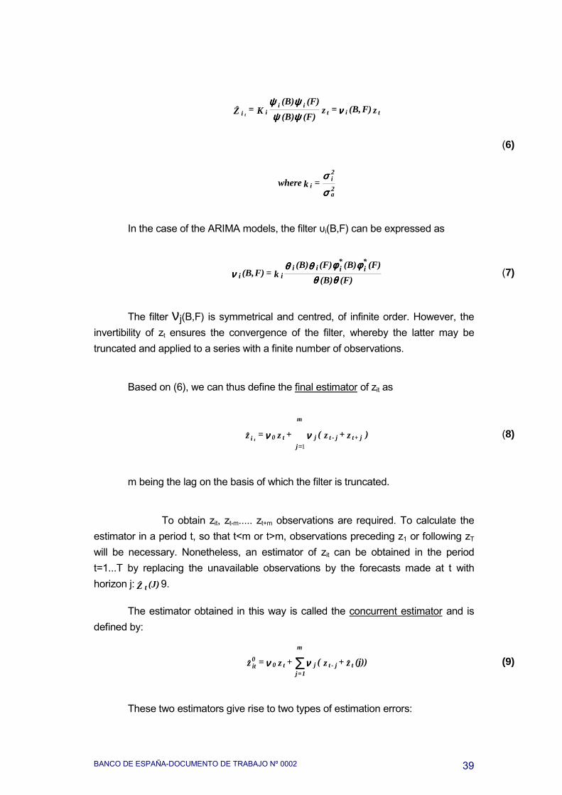
BANCO DE ESPAÑA-DOCUMENTO DE TRABAJO Nº 0002 39
In the case of the ARIMA models, the filter υi(B,F) can be expressed as
The filter νj(B,F) is symmetrical and centred, of infinite order. However, theinvertibility of zt ensures the convergence of the filter, whereby the latter may betruncated and applied to a series with a finite number of observations.
Based on (6), we can thus define the final estimator of zit as
m being the lag on the basis of which the filter is truncated.
To obtain zit, zt-m..... zt+m observations are required. To calculate theestimator in a period t, so that t<m or t>m, observations preceding z1 or following zT
will be necessary. Nonetheless, an estimator of zit can be obtained in the periodt=1...T by replacing the unavailable observations by the forecasts made at t withhorizon j: (J)Z tˆ 9.
The estimator obtained in this way is called the concurrent estimator and isdefined by:
These two estimators give rise to two types of estimation errors:
σσσσ
σσσσ
ννννψψψψψψψψψψψψψψψψ
2a
2i
i
titii
ii
=kwhere
zF)(B,=z(F)(B)(F)(B)
K=Z tˆ
(6)
(F)(B)(F)(B)(F)(B)
k=F)(B,*i
*iii
ii θθθθθθθθφφφφφφφφθθθθθθθθ
νννν (7)
=
m
jj+tj-tjt0i )z+z(+z=z t
1ˆ νννννννν (8)
(j))z+z(+z=z tj-tj
m
1=jt0
0it ˆˆ νννννννν Σ (9)

BANCO DE ESPAÑA-DOCUMENTO DE TRABAJO Nº 000240
Error in the final estimator error, owing to the truncation of the filter ν∞(L)
z -z=e ititf ˆ
Revision error, which gives an idea of the degree of revision recorded by theconcurrent estimator in relation to the final estimator, by using forecasts for the tails:
z -z=e 0ititr ˆˆ
Error in the total estimator(*), which is the sum of both errors. This is the errorcommitted by using the concurrent estimator z -z= e+ e=e 0
ititrft ˆ
(*) In new SEATS, given that the unobserved component, and hence its “final estimator error”, is never known,it is of little applied relevance. New SEATS uses “Total Estimation error” for testing signal of seasonally.“Revision error” to asses imprecision of the previous estimation in short-term monitoring of series.
BANCO DE ESPAÑA-DOCUMENTO DE TRABAJO Nº 0002 41
ANNEX 2: Complementary charts Chart A2.1
Spanish contribution to the monetary aggregates of euro area. Original adjusted Index of components
0.000
20.000
40.000
60.000
80.000
100.000
120.000
Jan-80
Jan-82
Jan-84
Jan-86
Jan-88
Jan-90
Jan-92
Jan-94
Jan-96
Jan-98
C urrency in circulat io n
0.000
20.000
40.000
60.000
80.000
100.000
120.000
Jan-80 Jan-82 Jan-84 Jan-86 Jan-88 Jan-90 Jan-92 Jan-94 Jan-96 Jan-98
Overnight dep osit s
0.000
20.000
40.000
60.000
80.000
100.000
120.000
140.000
Jan-80
Jan-82
Jan-84
Jan-86
Jan-88
Jan-90
Jan-92
Jan-94
Jan-96
Jan-98
Time dep osit s wit h agreed mat urit y up t wo years
0.000
20.000
40.000
60.000
80.000
100.000
120.000
Jan-80
Jan-82
Jan-84
Jan-86
Jan-88
Jan-90
Jan-92
Jan-94
Jan-96
Jan-98
R edeemable d epo sit s at no t ice up t hree mo nt hs
0.000
20.000
40.000
60.000
80.000
100.000
120.000
140.000
Jan-80 Jan-82 Jan-84 Jan-86 Jan-88 Jan-90 Jan-92 Jan-94 Jan-96 Jan-98
R e pur c ha se a gr e e me nt
0.000
20.000
40.000
60.000
80.000
100.000
120.000
140.000
160.000
180.000
Jan-80 Jan-82 Jan-84 Jan-86 Jan-88 Jan-90 Jan-92 Jan-94 Jan-96 Jan-98
M one y a nd ma r k e t f und sha r e / uni t s a nd mone y ma r k e t pa pe r
-4000.000
-2000.000
0.000
2000.000
4000.000
6000.000
8000.000
Jan-80
Jan-82
Jan-84
Jan-86
Jan-88
Jan-90
Jan-92
Jan-94
Jan-96
Jan-98
D ebt securit ies issued wit h mat urit y up t wo years
0.000
20.000
40.000
60.000
80.000
100.000
120.000
140.000
Jan-80 Jan-82 Jan-84 Jan-86 Jan-88 Jan-90 Jan-92 Jan-94 Jan-96 Jan-98
M 3 - M 2
BANCO DE ESPAÑA-DOCUMENTO DE TRABAJO Nº 000242
Chart A2.2Components of Spanish contribution to M3
Several rates of growth on S.a series (centred)
Currency
-10.0
0.0
10.0
20.0
30.0
40.0
50.0
60.0
Jan-90
Jan-91
Jan-92
Jan-93
Jan-94
Jan-95
Jan-96
Jan-97
Jan-98
Jan-99
T1,1 T3,1 T3,3 T1,12
O v e rnight de posits
-100.0
-50.0
0.0
50.0
100.0
150.0
200.0
250.0
Jan-90
Jan-91
Jan-92
Jan-93
Jan-94
Jan-95
Jan-96
Jan-97
Jan-98
Jan-99
T 1,1 T 3,1 T 3,3 T 1,12
T ime de posits
-40.0
-30.0
-20.0
-10.0
0.0
10.0
20.0
30.0
40.0
Jan-90
Jan-91
Jan-92
Jan-93
Jan-94
Jan-95
Jan-96
Jan-97
Jan-98
Jan-99
T1,1 T3,1 T3,3 T1,12
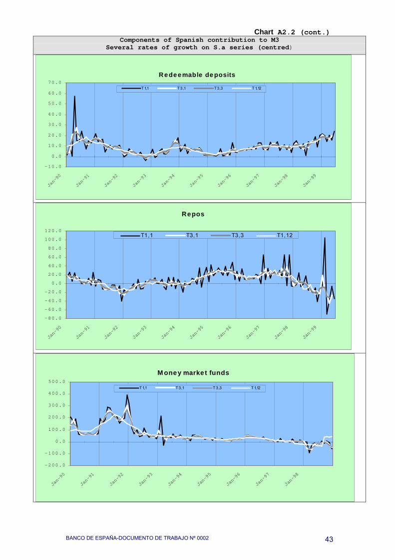
BANCO DE ESPAÑA-DOCUMENTO DE TRABAJO Nº 0002 43
Chart A2.2 (cont.)Components of Spanish contribution to M3
Several rates of growth on S.a series (centred)
Redeemable de posits
-10.0
0.0
10.0
20.0
30.0
40.0
50.0
60.0
70.0
Jan-90
Jan-91
Jan-92
Jan-93
Jan-94
Jan-95
Jan-96
Jan-97
Jan-98
Jan-99
T 1,1 T 3,1 T 3,3 T 1,12
Repos
-80.0
-60.0
-40.0
-20.0
0.0
20.0
40.0
60.0
80.0
100.0
120.0
Jan-90
Jan-91
Jan-92
Jan-93
Jan-94
Jan-95
Jan-96
Jan-97
Jan-98
Jan-99
T1,1 T3,1 T3,3 T1,12
M oney marke t funds
-200.0
-100.0
0.0
100.0
200.0
300.0
400.0
500.0
Jan-90
Jan-91
Jan-92
Jan-93
Jan-94
Jan-95
Jan-96
Jan-97
Jan-98
T1,1 T 3,1 T 3,3 T1,12
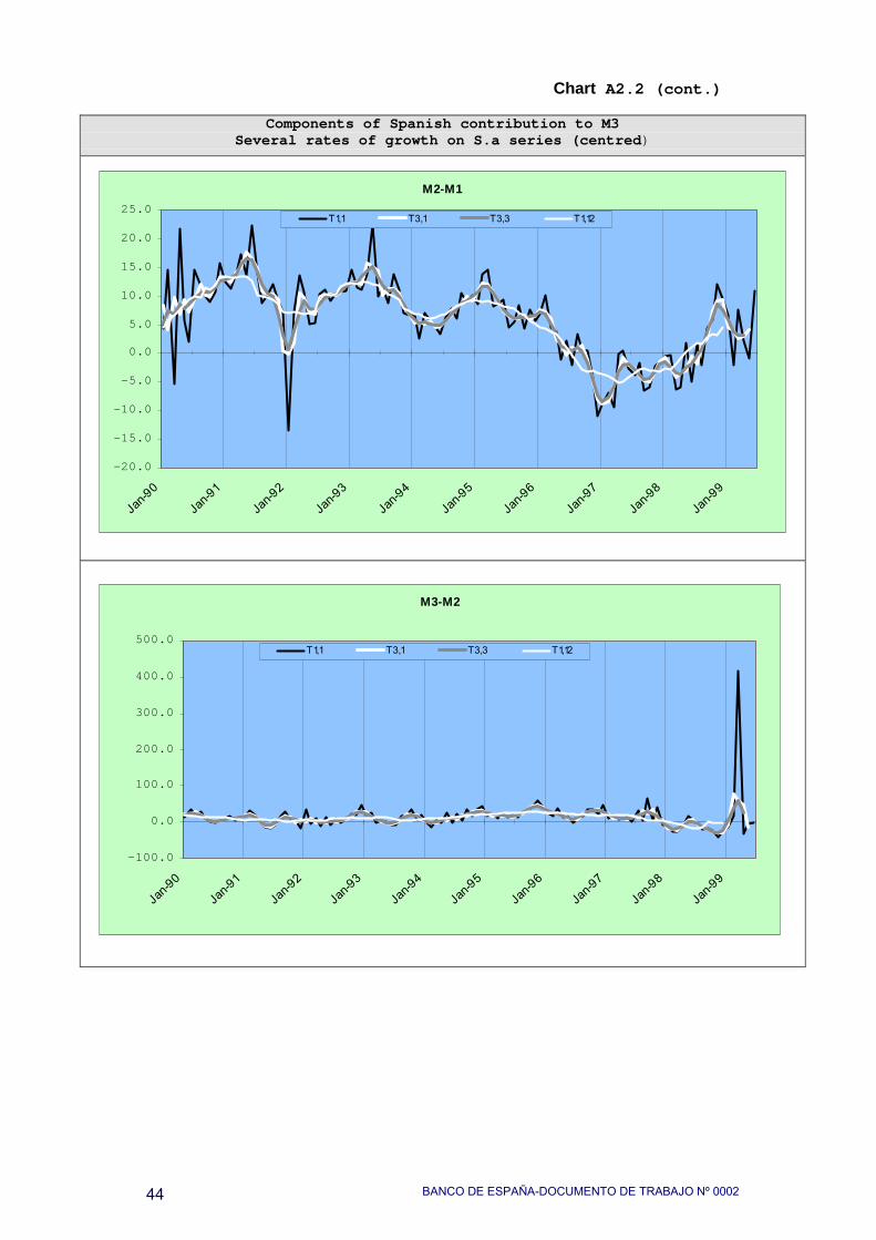
BANCO DE ESPAÑA-DOCUMENTO DE TRABAJO Nº 000244
Chart A2.2 (cont.)
Components of Spanish contribution to M3Several rates of growth on S.a series (centred)
M2-M1
-20.0
-15.0
-10.0
-5.0
0.0
5.0
10.0
15.0
20.0
25.0
Jan-9
0
Jan-91
Jan-9
2
Jan-9
3
Jan-9
4
Jan-9
5
Jan-9
6
Jan-9
7
Jan-9
8
Jan-9
9
T1,1 T3,1 T3,3 T1,12
M3-M2
-100.0
0.0
100.0
200.0
300.0
400.0
500.0
Jan-9
0
Jan-91
Jan-9
2
Jan-9
3
Jan-9
4
Jan-9
5
Jan-9
6
Jan-9
7
Jan-9
8
Jan-9
9
T1,1 T3,1 T3,3 T1,12