Searching stochastically generated multi-abstraction-level design spaces

Artificial Intelligence 129 (2001) 63–90

Searching stochastically generatedmulti-abstraction-level design spaces

Louis SteinbergDepartment of Computer Science, Rutgers University, New Brunswick, NJ 08903, USA

Received 15 February 2000; received in revised form 5 April 2001

Abstract

We present a new algorithm called Highest Utility First Search (HUFS) for searching treescharacterized by a large branching factor, the absence of a heuristic to compare nodes at differentlevels of the tree, and a child generator that is both expensive to run and stochastic in nature. Suchtrees arise naturally, for instance, in problems which involve candidate designs at several levels ofabstraction and which use stochastic optimizers such as genetic algorithms or simulated annealing togenerate a candidate at one level from a parent at the previous level. HUFS is applicable when thereis a class of related problems, from which many specific problems will need to be solved. This paperexplains the HUFS algorithm and presents experimental results comparing HUFS with alternativemethods. 2001 Elsevier Science B.V. All rights reserved.

Keywords: Heuristic search; Utility; Genetic algorithms; Stochastically generated trees; Abstraction levels

1. Introduction

In this paper we describe a new class of trees, which we call Stochastically-Generated(SG) trees, that arise naturally in Computer Aided Design. We describe an algorithm, calledHighest Utility First Search (HUFS), for searching such trees. HUFS is guided by estimatesit makes of the utility of searching the subtree under each existing node of the tree, andwe will also discuss how HUFS makes and uses these utility estimates. We will start bydescribing the class of trees and introducing some terminology related to utility.

E-mail address: [email protected] (L. Steinberg).

0004-3702/01/$ – see front matter 2001 Elsevier Science B.V. All rights reserved.PII: S0004-3702(01)0 01 05 -9

64 L. Steinberg / Artificial Intelligence 129 (2001) 63–90

1.1. Stochastically generated trees

In many kinds of engineering design tasks, the design process involves working withcandidate designs at several different levels of abstraction. For example, in designing amicroprocessor, one might start with an instruction set, implement the instructions as aseries of pipeline stages, implement the set of stages as a “netlist” defining how specificcircuit modules are to be wired together, etc. There are typically a combinatorially largenumber of ways a specific design at one level can be implemented at the next level down,but only a small, fixed set of levels.

The design space is a (virtual) tree. The nodes are the design alternatives at the variousabstraction levels, and the children of a parent design are all the designs at the next leveldown that implement that parent. Design in such a domain can be seen as a process ofsearching this tree for a high-quality leaf, e.g., for a leaf that represents a fast, cheapmicroprocessor.

Many complex design and optimization problems are typically structured this way incurrent practice. For instance, the generation of machine code in an optimizing compilerinvolves a series of stages in which the code may be represented first as a parse tree, thenas a sequence of three-address codes, and finally as machine code. Furthermore, the designof artifacts like aircraft and ships involves stages called preliminary, intermediate, and finaldesign, in which the artifact being designed is represented in successively greater detail.

Recently, a number of techniques for stochastic optimization have been shown to beuseful for finding good children of a design alternative. These techniques include simulatedannealing [10,19], genetic algorithms [1,7,12,13], and random-restart hill climbing [20].A design at one level is translated into a correct but poor design at the next level, and astochastic optimizer is used to improve this design.

An inherent feature of a stochastic method is that it can be run again and again on thesame inputs, each time potentially producing a different answer. These alternatives caneach be used as inputs to a similar process at the next lower level. Thus, these optimizerscan be seen as generating a tree of good design alternatives. These trees are much smallerthan the original trees, and consist only of relatively high-quality alternatives, but there canstill be significant variations in quality among alternatives and these trees can still havea large branching factor (in the thousands for examples we have looked at). So, there isstill a problem of controlling the search within the smaller tree, that is, for deciding whichalternative to generate a child from next.

This problem has a number of features that distinguish it from other tree searchproblems:

• The branching factor is high, as mentioned.• The cost to generate a single child is high, ranging from half a second to tens of

minutes in domains we have looked at.• The child-generation process is stochastic. We do not have an operator that will give

us all the children of a node, or even an operator which will generate children one byone in some systematic order.

• There is no concern for minimizing path length from the root to the goal node. All thatmatters is the quality of the design returned and the total amount of work involved infinding this design (i.e., the total path length of all arcs traversed in the search).

L. Steinberg / Artificial Intelligence 129 (2001) 63–90 65

Furthermore, while we will assume that, as in other tree search problems, we haveheuristic evaluation functions that can be used to compare design alternatives within alevel, we cannot assume that these functions are comparable across levels. In engineeringdomains such as microprocessor design, the alternatives at different levels are of entirelydifferent types (e.g., an instruction set versus a wiring diagram) and cannot easily becompared.

We will use the term Stochastically Generated (SG) trees to refer to trees with thesecharacteristics.

SG trees also arise when genetic algorithms (GAs) are used for engineering optimiza-tion. It is traditional for a GA to simply generate a sequence of populations, but it is possibleto save a population part way through the optimization and later restart the GA from thatpoint. Because of the stochastic nature of GAs, a different sequence of populations will begenerated each time the computation is restarted from the saved population. By saving anumber of populations and restarting a number of times, a tree can be generated in whichthe nodes are the saved populations and the operation that generates a child from a parentis to run the GA for some number of iterations. It has been shown [16] that searching sucha tree of populations can speed up optimization compared to just generating sequences ofpopulations.

It might seem that for a tree of GA populations we do have heuristic evaluation functionsthat are comparable across levels, since at all levels the alternatives are populations. In theempirical work discussed below, for instance, we use the quality of the best individualin a population as the evaluation function. However, while the numbers returned by thisfunction for populations at different levels are comparable in a formal sense, comparingthem does not give any useful guidance on which population to run the GA on next. It isnormal for populations lower in the tree (i.e., resulting from more iterations of the GA) tocontain better individuals than populations higher in the tree; indeed, in our experimentslower populations almost always have a better heuristic value than higher populations.Using these values to guide a standard best-first search results in going straight from theroot of the search tree to a leaf, with no branching. This is demonstrably [16] suboptimalin our test domain.

The problem is that, while populations at different levels are the same kind of objectsin a formal sense, they are still objects that are at different stages of the optimizationprocess, and a heuristic value which at an early stage signifies a good quality mayat a later stage signify a very poor quality. Thus, heuristic functions that simply lookat a population and compute some metric on it are unlikely to give useful searchguidance when compared across levels. Therefore, trees of populations can be seen asSG trees.

The approach HUFS takes to searching SG trees is to compute a “value” functionfor each level of the tree. The value function converts the heuristic score of a node,which is not comparable across levels, into an estimate of the quality of the searchprocess that starts with this node, which is comparable across levels. Thus, the questionof what determines the quality of a search becomes crucial. This issue will be discussednext.


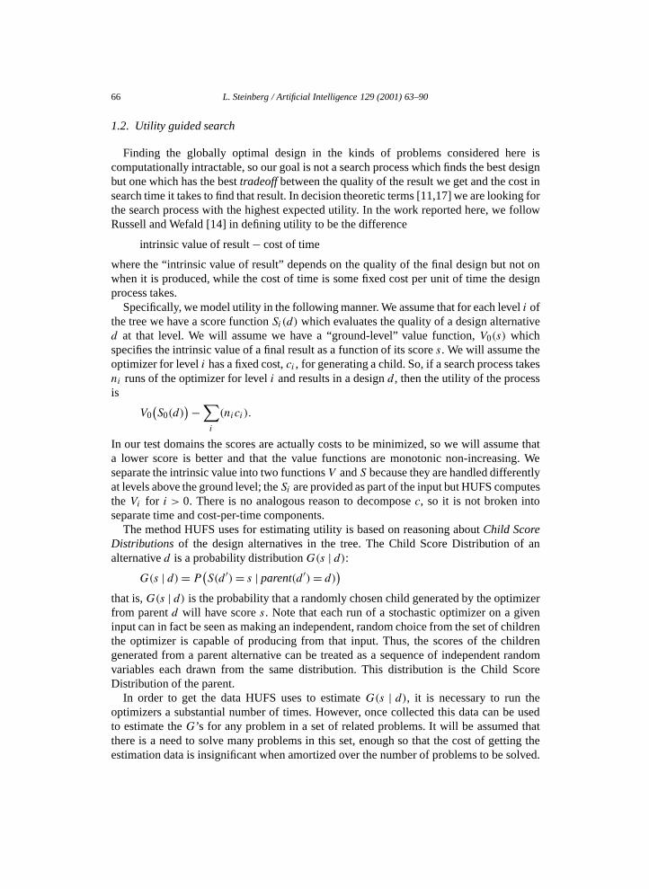
1.2. Utility guided search

Finding the globally optimal design in the kinds of problems considered here iscomputationally intractable, so our goal is not a search process which finds the best designbut one which has the best tradeoff between the quality of the result we get and the cost insearch time it takes to find that result. In decision theoretic terms [11,17] we are looking forthe search process with the highest expected utility. In the work reported here, we followRussell and Wefald [14] in defining utility to be the difference

intrinsic value of result − cost of time

where the “intrinsic value of result” depends on the quality of the final design but not onwhen it is produced, while the cost of time is some fixed cost per unit of time the designprocess takes.

Specifically, we model utility in the following manner. We assume that for each level i ofthe tree we have a score function Si(d) which evaluates the quality of a design alternatived at that level. We will assume we have a “ground-level” value function, V0(s) whichspecifies the intrinsic value of a final result as a function of its score s. We will assume theoptimizer for level i has a fixed cost, ci , for generating a child. So, if a search process takesni runs of the optimizer for level i and results in a design d , then the utility of the processis

V0(S0(d)

) −∑i

(nici).

In our test domains the scores are actually costs to be minimized, so we will assume thata lower score is better and that the value functions are monotonic non-increasing. Weseparate the intrinsic value into two functions V and S because they are handled differentlyat levels above the ground level; the Si are provided as part of the input but HUFS computesthe Vi for i > 0. There is no analogous reason to decompose c, so it is not broken intoseparate time and cost-per-time components.

The method HUFS uses for estimating utility is based on reasoning about Child ScoreDistributions of the design alternatives in the tree. The Child Score Distribution of analternative d is a probability distribution G(s | d):

G(s | d) = P(S(d ′) = s | parent(d ′) = d)

)that is, G(s | d) is the probability that a randomly chosen child generated by the optimizerfrom parent d will have score s. Note that each run of a stochastic optimizer on a giveninput can in fact be seen as making an independent, random choice from the set of childrenthe optimizer is capable of producing from that input. Thus, the scores of the childrengenerated from a parent alternative can be treated as a sequence of independent randomvariables each drawn from the same distribution. This distribution is the Child ScoreDistribution of the parent.

In order to get the data HUFS uses to estimate G(s | d), it is necessary to run theoptimizers a substantial number of times. However, once collected this data can be usedto estimate the G’s for any problem in a set of related problems. It will be assumed thatthere is a need to solve many problems in this set, enough so that the cost of getting theestimation data is insignificant when amortized over the number of problems to be solved.


The following sections will discuss, respectively,• the example design problem that has been our initial testbed,• the way HUFS estimates G(s | d),• the way it uses G(s | d) to estimate utilities and thus to guide the search,• the empirical test we have done and their results,• the related work in the literature,• the conclusions that can be drawn from the work presented here.

2. The example problem: Module placement

The initial example problem that we have been using to drive our work is the problemof positioning rectangular circuit modules on the surface of a VLSI chip: a given set ofrectangles must be placed in a plane in a way that minimizes the area of the bounding boxcircumscribed around the rectangles plus a factor that accounts for the area taken by thewires needed to connect the modules in a specified way.

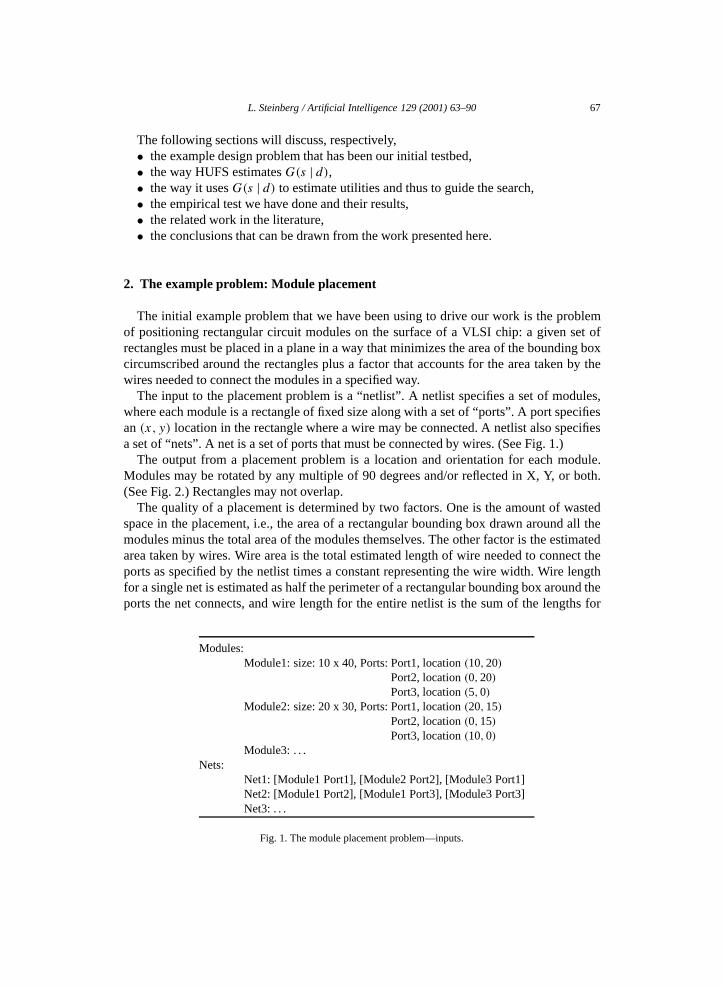
The input to the placement problem is a “netlist”. A netlist specifies a set of modules,where each module is a rectangle of fixed size along with a set of “ports”. A port specifiesan (x, y) location in the rectangle where a wire may be connected. A netlist also specifiesa set of “nets”. A net is a set of ports that must be connected by wires. (See Fig. 1.)

The output from a placement problem is a location and orientation for each module.Modules may be rotated by any multiple of 90 degrees and/or reflected in X, Y, or both.(See Fig. 2.) Rectangles may not overlap.

The quality of a placement is determined by two factors. One is the amount of wastedspace in the placement, i.e., the area of a rectangular bounding box drawn around all themodules minus the total area of the modules themselves. The other factor is the estimatedarea taken by wires. Wire area is the total estimated length of wire needed to connect theports as specified by the netlist times a constant representing the wire width. Wire lengthfor a single net is estimated as half the perimeter of a rectangular bounding box around theports the net connects, and wire length for the entire netlist is the sum of the lengths for

Modules:Module1: size: 10 x 40, Ports: Port1, location (10,20)

Port2, location (0,20)Port3, location (5,0)

Module2: size: 20 x 30, Ports: Port1, location (20,15)Port2, location (0,15)Port3, location (10,0)

Module3: . . .Nets:

Net1: [Module1 Port1], [Module2 Port2], [Module3 Port1]Net2: [Module1 Port2], [Module1 Port3], [Module3 Port3]Net3: . . .

Fig. 1. The module placement problem—inputs.


Module1: XY: (15, 0), Rotation: 90 degrees, Reflect X: false, Reflect Y: true

Module2: . . .

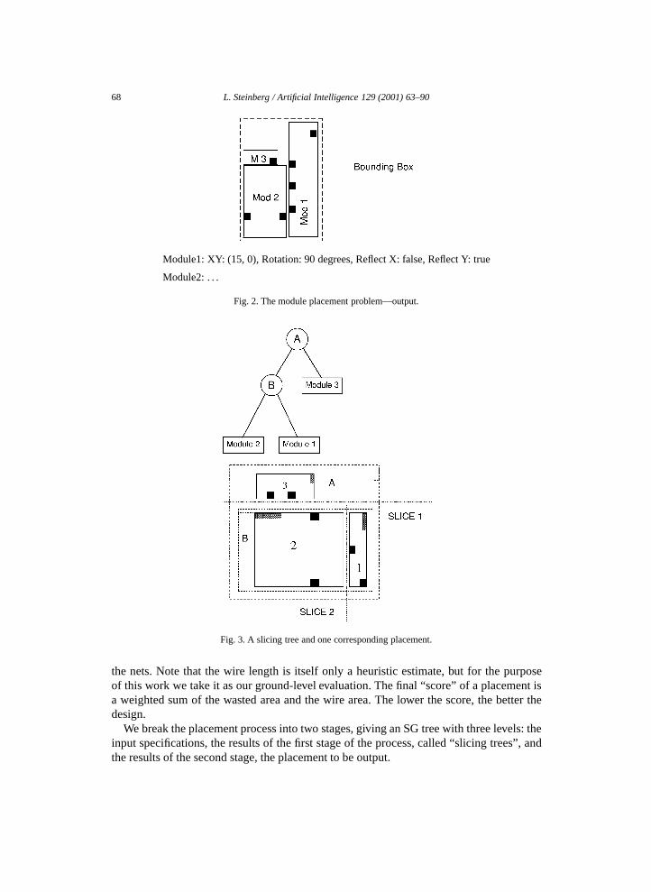
Fig. 2. The module placement problem—output.

Fig. 3. A slicing tree and one corresponding placement.

the nets. Note that the wire length is itself only a heuristic estimate, but for the purposeof this work we take it as our ground-level evaluation. The final “score” of a placement isa weighted sum of the wasted area and the wire area. The lower the score, the better thedesign.

We break the placement process into two stages, giving an SG tree with three levels: theinput specifications, the results of the first stage of the process, called “slicing trees”, andthe results of the second stage, the placement to be output.


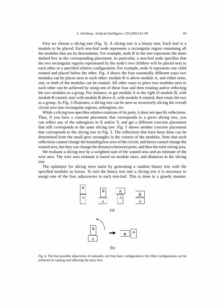
First we choose a slicing tree (Fig. 3). A slicing tree is a binary tree. Each leaf is amodule to be placed. Each non-leaf node represents a rectangular region containing allthe modules that are its descendants. For example, node B in the tree represents the innerdashed box in the corresponding placement. In particular, a non-leaf node specifies thatthe two rectangular regions represented by the node’s two children will be placed next toeach other in a specified relative configuration. For example, node A represents one childrotated and placed below the other. Fig. 4 shows the four essentially different ways twomodules can be places next to each other: module B is above module A, and either none,one, or both of the modules can be rotated. All other ways to place two modules next toeach other can be achieved by using one of these four and then rotating and/or reflectingthe two modules as a group. For instance, to get module A to the right of module B, withmodule B rotated, start with module B above A, with module A rotated, then rotate the twoas a group. As Fig. 3 illustrates, a slicing tree can be seen as recursively slicing the overallcircuit area into rectangular regions, subregions, etc.

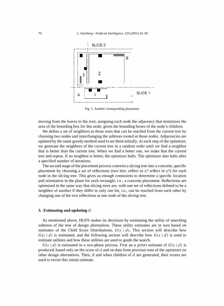
While a slicing tree specifies relative rotations of its parts, it does not specify reflections.Thus, if you have a concrete placement that corresponds to a given slicing tree, youcan reflect any of the subregions in X and/or Y, and get a different concrete placementthat still corresponds to the same slicing tree. Fig. 5 shows another concrete placementthat corresponds to the slicing tree in Fig. 3. The reflections that have been done can bedetermined from the small grey rectangles in the corners of the modules. Note that suchreflections cannot change the bounding box area of the circuit, and hence cannot change thewasted area, but they can change the distances between ports, and thus the total wiring area.

We evaluate a slicing tree by a weighted sum of the wasted area and an estimate of thewire area. The wire area estimate is based on module sizes, and distances in the slicingtree.

The optimizer for slicing trees starts by generating a random binary tree with thespecified modules as leaves. To turn the binary tree into a slicing tree it is necessary toassign one of the four adjacencies to each non-leaf. This is done in a greedy manner,

(a)

(b)

Fig. 4. The four possible adjacencies of subnodes. (a) Four basic configurations; (b) Other configurations can beachieved by rotating and reflecting the basic four.


Fig. 5. Another corresponding placement.

moving from the leaves to the root, assigning each node the adjacency that minimizes thearea of the bounding box for this node, given the bounding boxes of the node’s children.

We define a set of neighbors as those trees that can be reached from the current tree bychoosing two nodes and interchanging the subtrees rooted at those nodes. Adjacencies areupdated by the same greedy method used to set them initially. At each step of the optimizer,we generate the neighbors of the current tree in a random order until we find a neighborthat is better than the current tree. When we find a better one, we make that the currenttree and repeat. If no neighbor is better, the optimizer halts. The optimizer also halts aftera specified number of iterations.

The second stage of the placement process converts a slicing tree into a concrete, specificplacement by choosing a set of reflections (two bits: reflect in x? reflect in y?) for eachnode in the slicing tree. This gives us enough constraints to determine a specific locationand orientation in the plane for each rectangle, i.e., a concrete placement. Reflections areoptimized in the same way that slicing trees are, with one set of reflections defined to be aneighbor of another if they differ in only one bit, i.e., can be reached from each other bychanging one of the two reflections at one node of the slicing tree.

3. Estimating and updating G

As mentioned above, HUFS makes its decisions by estimating the utility of searchingsubtrees of the tree of design alternatives. These utility estimates are in turn based onestimates of the Child Score Distributions, G(s | d). This section will describe howG(s | d) is estimated, and the following section will describe how G(s | d) is used toestimate utilities and how these utilities are used to guide the search.

G(s | d) is estimated in a two-phase process. First an a priori estimate of G(s | d) isproduced, based only on the score of d and on data from previous runs of the optimizer onother design alternatives. Then, if and when children of d are generated, their scores areused to revise this initial estimate.


In following subsections we will describe how we make the a priori estimate of G(s | d),then we will describe how this estimate is revised using the child scores. First, however,we will discuss our approach to modeling uncertainty about distributions.

3.1. Representing uncertainty about distributions

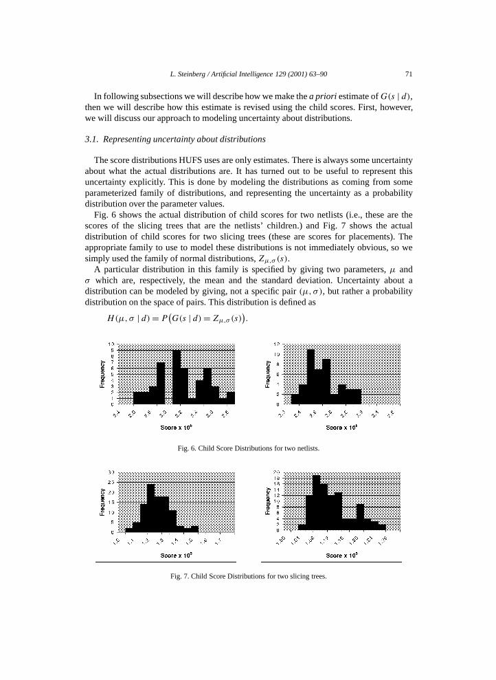
The score distributions HUFS uses are only estimates. There is always some uncertaintyabout what the actual distributions are. It has turned out to be useful to represent thisuncertainty explicitly. This is done by modeling the distributions as coming from someparameterized family of distributions, and representing the uncertainty as a probabilitydistribution over the parameter values.

Fig. 6 shows the actual distribution of child scores for two netlists (i.e., these are thescores of the slicing trees that are the netlists’ children.) and Fig. 7 shows the actualdistribution of child scores for two slicing trees (these are scores for placements). Theappropriate family to use to model these distributions is not immediately obvious, so wesimply used the family of normal distributions, Zµ,σ (s).

A particular distribution in this family is specified by giving two parameters, µ andσ which are, respectively, the mean and the standard deviation. Uncertainty about adistribution can be modeled by giving, not a specific pair (µ,σ ), but rather a probabilitydistribution on the space of pairs. This distribution is defined as

H(µ,σ | d) = P(G(s | d) = Zµ,σ (s)

).

Fig. 6. Child Score Distributions for two netlists.

Fig. 7. Child Score Distributions for two slicing trees.


That is, H(µ,σ | d) is the probability that G(s | d) is the particular normal distributionspecified by the pair (µ,σ ).

G(s | d), the estimated probability of a child having score s, can be calculated from H :

G(s | d) =∫µ

∫σ

H(µ,σ | d)Zµ,σ (s)dσ dµ. (1)

3.2. The initial estimate of G

Each estimate HUFS makes of G is generated via Eq. (1) from a corresponding estimateof H . Thus, to get its initial estimate, G0(s | d), HUFS calculates H0(µ,σ | d), its initialestimate of H .

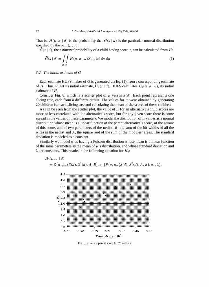
Consider Fig. 8, which is a scatter plot of µ versus S(d). Each point represents oneslicing tree, each from a different circuit. The values for µ were obtained by generating20 children for each slicing tree and calculating the mean of the scores of these children.

As can be seen from the scatter plot, the value of µ for an alternative’s child scores aremore or less correlated with the alternative’s score, but for any given score there is somespread in the values of these parameters. We model the distribution of µ values as a normaldistribution whose mean is a linear function of the parent alternative’s score, of the squareof this score, and of two parameters of the netlist: B , the sum of the bit-widths of all thewires in the netlist and A, the square root of the sum of the modules’ areas. The standarddeviation is modeled as a constant.

Similarly we model σ as having a Poisson distribution whose mean is a linear functionof the same parameters as the mean of µ’s distribution, and whose standard deviation andλ are constants. This results in the following equation for H0:

H0(µ,σ | d)= Z

(µ,µµ

(S(d), S2(d),A,B

), σµ

)P

(σ,µσ

(S(d), S2(d),A,B

), σσ , λ

),

Fig. 8. µ versus parent score for 20 netlists.


where Z(x,µ,σ) is the standard normal density function with mean µ and standarddeviation σ , evaluated at x , P(x,µ,σ,λ) is the Poisson density function, with mean,standard deviation, and lambda given by µ, σ , and λ, and the functions µµ, and µσ arelinear functions.

The coefficients of the linear functions, as well as the constants σµ, σσ , and λ, areestimated based on data both from previous work on the current problem (the currentcircuit) and from previous problems. To do this estimation. we start by finding twentydesign alternatives that already have children. These parents are taken first from siblings ofthe alternative whose H0 we are computing. If there are not enough siblings, we use otheralternatives at the same level in the current problem, and finally we use alternatives froma set of calibration runs (see below). For each parent we calculate the mean and standarddeviation of its childrens’ scores, and use this data in a least-squares fit to estimate thecoefficients and constants needed for calculating H0.

Given H0, we can calculate G using Eq. (1).

3.3. Calibration data

The pool of design alternatives from which we estimate the coefficients of H0 isinitialized from a set of calibration data. For each of a number of randomly generatedproblems a parent design alternative is generated at each level but the lowest (i.e., forthe rectangle placement problems, a netlist and a slicing tree are generated for each of20 circuits). Then 15 children are generated from each parent in order to determine thevalues of µ and σ for the parent’s Child Score Distribution.

Note that this gives a substantial startup cost for applying these methods in a newdomain, but that this cost can be amortized over all subsequent use of the method in thatdomain. Also note that this cost grows linearly with the number of levels. If there had beena level below placements, we would have needed to generate 15 children at this level fromone placement per circuit for each of the 15 circuits.

3.4. Updating G

Each time we generate a child from alternative d and determine that child’s score, wecan revise H using the standard Bayesian formula,

Hi(µ,σ) = P(µ,σ | si ) = P(si | µ,σ) ∗ P(µ,σ)

P (si)= Zµ,σ (si) ∗Hi−1(µ,σ )

Gi−1(si | d) ,

where Hi is our estimate of H after seeing i children, H0 is our a priori H as above,Gi−1(si | d) is the G derived from Hi−1, and si is the score of the ith child of d . From Hi

we then get Gi via Eq. (1).

4. HUFS

This section describes the HUFS algorithm. One way to understand HUFS is to viewit as the result of applying a series of modifications to a simple greedy algorithm we will


refer to simply as “Greedy”. We will describe Greedy and the sequence of improvementswhich leads from Greedy to HUFS.

4.1. Greedy

In practice, an engineer faced with a design task like those discussed above may takethe following simple approach: work from top down, generating a small, fixed number ofalternatives at a given level. Choose the best of the designs generated at this level, usingsome heuristic that compares alternatives within the level, and then use this best design asthe (only) parent from which to generate designs at the next level. This process is carriedout level by level until the resulting designs are at the lowest level. The best of these ground-level designs is then output as the result of the search. We call this method “Greedy”because it proceeds top-down, without ever looking back to reconsider the choices madeat higher levels.

This method has the advantages of simplicity, low storage cost, and predictableexecution time, but if G(s | d) is known it is possible devise methods which have higherexpected utility.

4.2. Optimal Stopping—single level

Let us start with a simplified situation, and assume that there is only one level ofoptimization (and thus two levels of representation: the problem specification is the root ofthe search tree and its children are solutions, i.e., leaves).

Since the result of one run of the optimizer does not affect the following runs, we canview the scores of successive children as being independently drawn from some fixeddistribution. This allows us to apply a result from the area of statistics known as OptimalStopping [5,15].

Suppose that we generate n children from the root, and that they have scores s1 . . . sn.The utility of this process is then the value of the best child we find minus the cost of doingn runs: V (min1�i�n si) − cn. In the single-level case our only decision is whether to stopand return the best child so far as our result, or to generate another child. When should westop?

Note that generating another child only improves our utility if that new child is betterthan the best so far, enough better to balance the cost of generating the new child. Let sb bethe best child score we’ve seen so far. The better (lower) sb is, the less likely a new child isto be an improvement, and the smaller each improvement will be. Thus, the average benefitfrom generating a new child decreases as sb gets better. But the cost of generating a childis constant, so as sb decreases, the net incremental utility of generating one more childalso decreases. It can be shown [5,15] that we get the highest overall utility for the designprocess if we keep generating children until the incremental utility of generating anotherchild is negative. Note that the incremental utility is a local measure, i.e., the utility oftaking one more child, but that stopping when this local utility becomes negative actuallyleads to the optimal global utility for the overall design process.

If we know the Child Score Distribution G, the value function V , and the cost c we cancalculate ∆U(sb), the incremental utility for a given current best child score sb . It is the


difference between the value of the best child we will have after one more optimizer runand the value of the current best child, minus c. Since we do not yet know the score of thenext child (and since we don’t even know G, but rather only our estimate, G), we take theaverage over all possible scores, weighted by G):

∆U(sb) =∞∫

0

(max

(V (s),V (sb)

) − V (sb) − c)G(s | d)ds

=sb∫

0

(V (s) − V (sb)

)G(s | d)ds − c.

(Remember that we are assuming V is monotonic non-increasing. If it is not, we assume itcan be made monotonic by adjusting the score function so that it is better predictor of V .)

So, the first improvement for a single-level search is to not generate a fixed numberof children at each level, but rather to generate children until ∆U(sb) � 0. Since ∆U ismonotonic in sb , this is equivalent to stopping as soon as sb � t , where the threshold scoret is the score such that ∆U(t) = 0.

Given this stopping criterion, we can calculate the expected value and expected cost ofthe whole (single-level) process. First, consider the expected value of the process. This isjust the expected value of the V function applied to the score of the resulting design. Thatis, if we let dr be the alternative finally returned as the result of the design process, thenthe expected value of the process is E(V (S(dr))) where E is expected value. S(dr) mustbe less (better) than t , our threshold score for stopping, so

P(S(dr) = sr

) = P(S(d0) = sr | S(d0) � t

) = G(sr )∫ t

0 G(s | d)ds,

where d0 is any ground-level object. So the expected value of the final resulting design is

E(V (S(dr ))

) =∫ t

0 G(s′ | d)V (s′)ds′∫ t

0 G(s′ | d)ds.

The probability that any one run of the optimizer will find a design with score � t is just∫ t

0 G(s | d)ds, so the average number of runs until we find such a design is

E(n) = 1/

t∫0

G(s | d)ds.

So, for a single-level search, the overall utility of the search, US , is

US(d) = E(V (S(dr))

) − cE(n) =∫ t

0 V (s)G(s | d)ds∫ t

0 G(s)ds− c∫ t

0 G(s)ds

assuming we use the optimal stopping criterion.


It is interesting to note that if one takes the definition of t , ∆U(t) = 0, substitutes in thedefinition of ∆U , and solves for V (t), the result is

V (t) =∫ t

0 G(s | d)V (s)ds − c∫ t

0 G(s | d)ds= US(d).

That is, the utility of the search is just the value of the threshold score. We stop for anyscore better than t , so E(V (S(dr ))), the value of our result, must be more than V (t) bysome amount. It turns out that the cost c ∗E(n) exactly balances this and brings the utility(which is value − cost) back down to V (t).

4.3. Optimal Stopping—multiple levels

Now let us consider extending these results to multiple levels. If we had the G’s, V , andc at each level we could treat each level as a separate single-level problem and apply thesingle-level method above: we would start at the root, generating children from it as if thiswere a single-level problem, until the single-level method said to stop. Then we would takethe best child we had generated and use it as the parent in a similar process at the next leveldown, and so on.

In fact, we assume that we do have G(s | d), and c for each level. The value of c canbe estimated empirically if need be, and the method for calculating G(s | d) was describedabove. Also, we assume that V0, the value of a final result, is provided by the user. However,this still leaves us in need of V for the other levels. What is the value of a design alternativesuch as a slicing tree, which is not at the lowest level?

An alternative at any level above the lowest has no value in and of itself. Its only valuecomes from the fact that it can be used to generate children, grandchildren, etc. That is, itsnet value is the value of the final design we will get if we search under it, minus the cost ofdoing that search. In other words, the value of a non-ground design alternative is the utilityof searching under it:

Vi

(Si(d)

) = USi(d).

(Note that if we define “searching under” a ground-level design as just returning thatdesign, this equation also applies at the ground level, since in this case dr = d and n = 0,so US0(d) = V0(S0(dr)) − n ∗ c0 = V0(S0(d)).)

Then we can calculate the value of an alternative di at level i with score sp as

Vi(sp) = Vi−1(ti−1),

where ti−1 is the threshold score at which we stop generating children of di , that is, ti−1 isdefined such that

ti−1∫0

(Vi−1(s) − Vi−1(ti−1)

)Gi(s | sp)ds = ci−1.

So if V0 is given by the user we can calculate V1, V2, and so on. If we do this, it turnsout that, for instance, the utility we calculate for a netlist is not just a utility for generatingslicing trees from that netlist, it is also the utility of the whole search under the netlist all


the way down to the placement level, assuming we use Greedy with Optimal Stopping asour search algorithm. For example,

US2(d) = E(US1(dr1)

) − c1 ∗ n1

= E(US0(dr0) − c0 ∗ n0

) − c1 ∗ n1

= V0(dr0) − (c0 ∗ n0 + c1 ∗ n1).

4.4. Greedy with Updating, Pseudo-Optimal Stopping, and Parent Changing

So far in describing HUFS we have assumed that the G’s were constant. As describedabove, however, G(s | d) needs to be updated each time we generate a child from d . Aswe generate children from a parent and update its utility, it often happens that the childscores are worse than expected initially, and updating the parent’s G reduces our estimateof its utility, reduces it so much that this parent no longer has the highest estimated utilityamong its siblings. In this case it makes sense to switch parents. That is, when working ata given level it makes sense to let the parent at each step be the alternative at that level thatcurrently looks best, i.e., has the highest estimated utility. Doing so gives us Greedy withUpdating, Pseudo-Optimal Stopping, and Parent Changing.

4.5. Highest Utility First Search (HUFS)

There are two final steps to take to convert Greedy with Updating, Pseudo-OptimalStopping, and Parent Changing into Highest Utility First Search. Notice that, even thoughthe score functions Si and Sj at levels i and j = i cannot be compared, the utility estimateUS(d) is comparable across all levels of the tree: the utility of a netlist is the expectedutility of searching under it for a placement, as is the utility of a slicing tree. The utility ofa placement is just its value, since no search cost needs to be paid to turn a placement intoa placement.

Since all utilities are comparable, there is no reason to confine ourselves to the currentlevel when we are looking for the best parent to generate the next child from. We shouldlook at all design alternatives at all levels, and choose the one with the highest utility. If thealternative with the highest utility is at the lowest (ground) level, this means that the actionof returning it as the answer right now, with no further computing, has higher utility thansearching under anything at any higher level, so that is what we should do: stop and returnit.

This amounts to Best First Search where best is determined by the utility estimates,hence our naming the algorithm Highest Utility First Search. Note that the utility estimateis still based on Greedy with Pseudo-Optimal Stopping (but without Parent Changing); itdoes not reflect the actual search algorithm. An interesting direction for future work is tofind a way to make the utility estimates reflect the actual HUFS algorithm.

There is one final complication: empirical tests of the algorithm as described so farshowed that occasionally HUFS would underestimate the mean of an alternative’s G oroverestimate its standard deviation, and would keep generating children well past the actualoptimal stopping point, until it finally corrected the estimate. In order to prevent this, anadditional mechanism was added to HUFS. When HUFS estimates the utility of a design


alternative d , it also calculates how many child scores need to be drawn from G(s | d) inorder to have a probability of 0.95 that at least one of the children has a score less than t . Ifthis many children have already been generated without finding one with a score less thant , HUFS takes this as evidence that its G(s | d) is inaccurate, and marks d as “cut off”.Alternatives marked as cut off are ignored when HUFS looks for the alternative with thehighest utility.

4.6. Summary of HUFS

We started with a single-level search and precise knowledge of G, and used the stoppingrule from the statistics literature which is optimal for this case. We extended it to multiplelevels (which the literature does not do) to get Greedy with Optimal Stopping. Wethen moved to the actual situation where we have only imprecise knowledge of G, andrepresented that knowledge by a probability distribution on G’s parameters. This led tothe need to update G after we generate each child and see its score. This updating maygive the parent a worse score than one of its siblings, so the next modification was thatwhen we generated a child we used the parent with the highest utility among the currentparent and its siblings. We saw that the utility estimate was a heuristic estimation of howgood each alternative in the tree was and could be compared across levels, giving us bestfirst search where best means highest utility, i.e., HUFS. Finally, if HUFS has generatedso many children from an alternative that, based on G, it should by now have found achild good enough to make it stop generating children from this parent, then HUFS stopsgenerating children from it even if it has not found such a child.

5. Empirical test

We have tested HUFS on two problems: the rectangle placement problem describedabove and a problem involving genetic algorithms and the conceptual design of an airplane.We will describe the tests and results from the rectangle placement problem, and thendescribe the GA problem, how we tested HUFS on it, and the results.

5.1. Rectangle placement

The test problems in the rectangle placement task were a set of randomly generatednetlists. Each netlist had 20 modules. We rather arbitrarily chose the value function at thelowest level to be V0(s) = 1e6 − s. The cost to generate a child was set to the average timein seconds it took to run the optimizer (0.3 for a placement, 1.9 for a slicing tree) times a“cost factor”. In our tests we used four different cost factors: 1500, 1000, 500, and 250.

The calibration data was generated by taking 20 netlists and generating 15 slicingtrees for each, then taking one of those slicing trees for each netlist and generating15 placements. For each test run, one of these problems was used as the problem to solveand the other 19 were used to provide calibration data.

For each test problem, for each cost factor, we ran HUFS five times. We computed timefor a run by multiplying the number of times each optimizer was run by the average run-time for that optimizer and summing over the optimizers. We averaged the run-times and


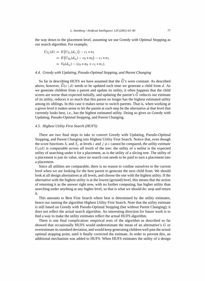
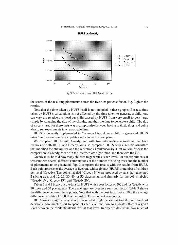
Fig. 9. Score versus time: HUFS and Greedy.

the scores of the resulting placements across the five runs per cost factor. Fig. 9 gives theresults.

Note that the time taken by HUFS itself is not included in these graphs. Because timetaken by HUFS’s calculations is not affected by the time taken to generate a child, onecan vary the relative overhead per child caused by HUFS from very small to very largesimply by changing the size of the circuits, and thus the time to generate a child. The sizeof circuits used for these tests was a compromise between having realistic sizes and beingable to run experiments in a reasonable time.

HUFS is currently implemented in Common Lisp. After a child is generated, HUFStakes 1 to 5 seconds to do its updates and choose the next parent.

We compared HUFS with Greedy, and with two intermediate algorithms that havefeatures of both HUFS and Greedy. We also compared HUFS with a genetic algorithmthat modified the slicing tree and the reflections simultaneously. First we will discuss thecomparison to Greedy, then with the intermediate algorithms, and then with the GA.

Greedy must be told how many children to generate at each level. For our experiments, itwas run with several different combinations of the number of slicing trees and the numberof placements to be generated. Fig. 9 compares the results with the results from HUFS.Each point represents the average of five runs with a given c (HUFS) or number of childrenper level (Greedy). The points labeled “Greedy 5” were produced by runs that generated5 slicing trees and 10, 20, 30, 40, or 50 placements, and similarly for the points labeled“Greedy 10”, “Greedy 15”, and “Greedy 20”.

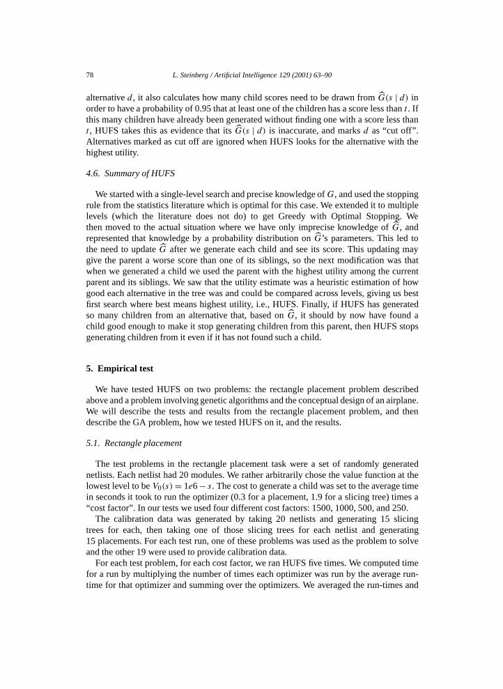
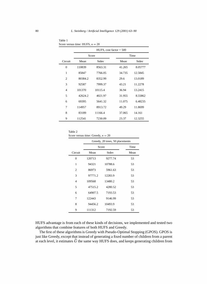
Tables 1 and 2 break out the data for HUFS with a cost factor of 500 and for Greedy with20 trees and 50 placements. There averages are over five runs per circuit. Table 3 showsthe difference between these points. Note that with the cost factor set at 500, the averagedifference in utility of 15,000 is the cost of 30 seconds of computing.

HUFS uses a single mechanism to make what might be seen as two different kinds ofdecisions: how much effort to spend at each level and how to allocate effort at a givenlevel between the available alternatives at that level. In order to determine how much of


Table 1Score versus time: HUFS, n = 20

HUFS, cost factor = 500

Score Time

Circuit Mean Stdev Mean Stdev

0 110839 8563.31 41.265 8.05777

1 85847 7766.05 34.735 12.5845

2 80384.2 8352.99 29.6 13.0189

3 92587 7999.37 43.21 11.2278

4 101370 10115.4 36.94 13.2415

5 42624.2 4021.97 31.955 8.55862

6 69395 5641.32 11.075 6.48235

7 114957 8913.72 49.29 11.8699

8 83189 11166.4 37.065 14.161

9 112541 7230.09 23.37 12.3255

Table 2Score versus time: Greedy, n = 20

Greedy, 20 trees, 50 placements

Score Time

Circuit Mean Stdev Mean

0 120713 9277.74 53

1 94321 10788.6 53

2 86973 5961.63 53

3 97771.2 12283.9 53

4 109568 13480.2 53

5 47515.2 4280.52 53

6 64907.5 7193.53 53

7 122443 9146.99 53

8 94456.2 10493.9 53

9 111312 7192.59 53

HUFS advantage is from each of these kinds of decisions, we implemented and tested twoalgorithms that combine features of both HUFS and Greedy.

The first of these algorithms is Greedy with Pseudo-Optimal Stopping (GPOS). GPOS isjust like Greedy, except that instead of generating a fixed number of children from a parentat each level, it estimates G the same way HUFS does, and keeps generating children from


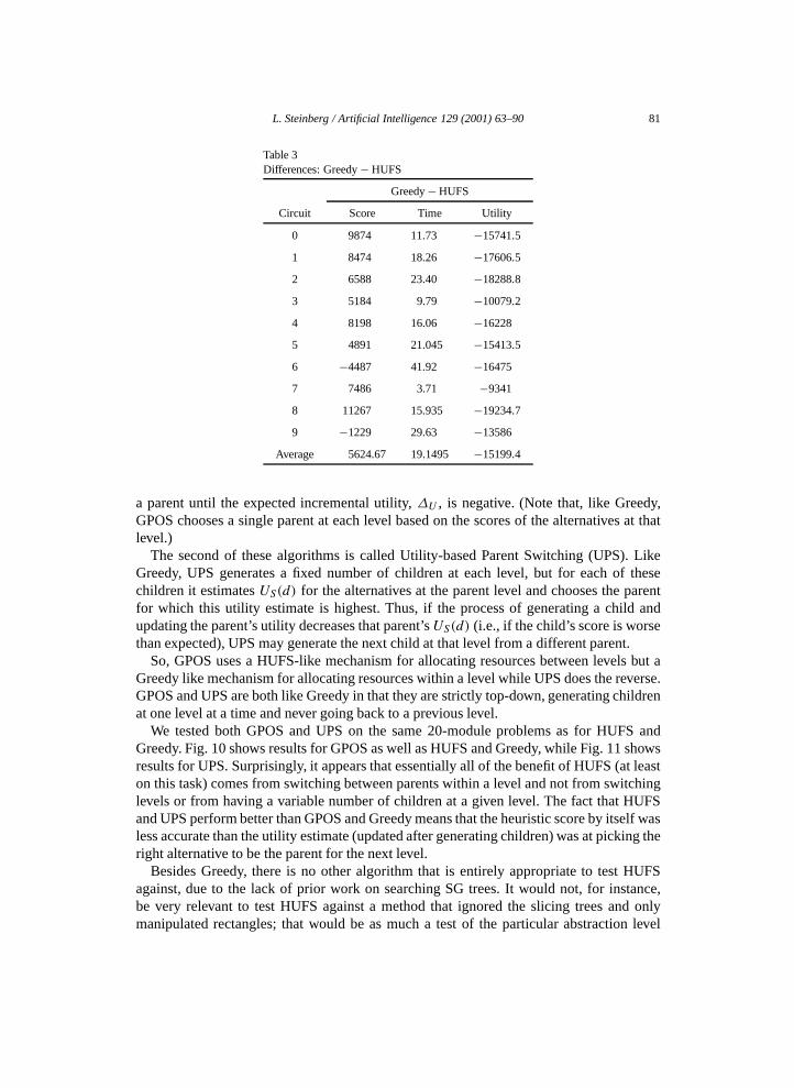
Table 3Differences: Greedy − HUFS

Greedy − HUFS

Circuit Score Time Utility

0 9874 11.73 −15741.5

1 8474 18.26 −17606.5

2 6588 23.40 −18288.8

3 5184 9.79 −10079.2

4 8198 16.06 −16228

5 4891 21.045 −15413.5

6 −4487 41.92 −16475

7 7486 3.71 −9341

8 11267 15.935 −19234.7

9 −1229 29.63 −13586

Average 5624.67 19.1495 −15199.4

a parent until the expected incremental utility, ∆U , is negative. (Note that, like Greedy,GPOS chooses a single parent at each level based on the scores of the alternatives at thatlevel.)

The second of these algorithms is called Utility-based Parent Switching (UPS). LikeGreedy, UPS generates a fixed number of children at each level, but for each of thesechildren it estimates US(d) for the alternatives at the parent level and chooses the parentfor which this utility estimate is highest. Thus, if the process of generating a child andupdating the parent’s utility decreases that parent’s US(d) (i.e., if the child’s score is worsethan expected), UPS may generate the next child at that level from a different parent.

So, GPOS uses a HUFS-like mechanism for allocating resources between levels but aGreedy like mechanism for allocating resources within a level while UPS does the reverse.GPOS and UPS are both like Greedy in that they are strictly top-down, generating childrenat one level at a time and never going back to a previous level.

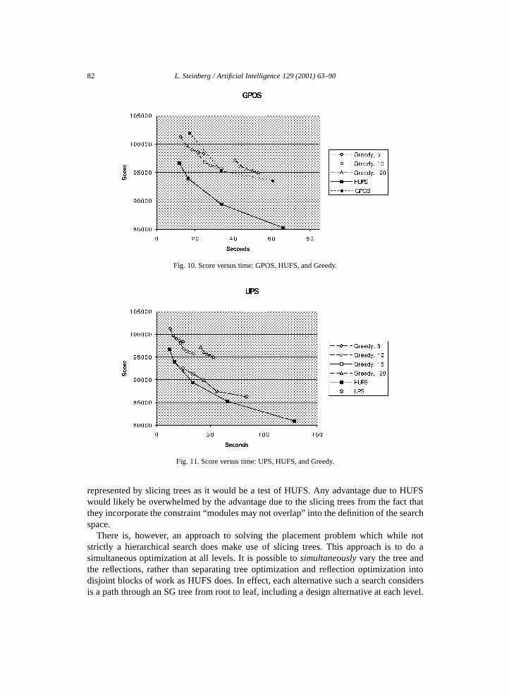
We tested both GPOS and UPS on the same 20-module problems as for HUFS andGreedy. Fig. 10 shows results for GPOS as well as HUFS and Greedy, while Fig. 11 showsresults for UPS. Surprisingly, it appears that essentially all of the benefit of HUFS (at leaston this task) comes from switching between parents within a level and not from switchinglevels or from having a variable number of children at a given level. The fact that HUFSand UPS perform better than GPOS and Greedy means that the heuristic score by itself wasless accurate than the utility estimate (updated after generating children) was at picking theright alternative to be the parent for the next level.

Besides Greedy, there is no other algorithm that is entirely appropriate to test HUFSagainst, due to the lack of prior work on searching SG trees. It would not, for instance,be very relevant to test HUFS against a method that ignored the slicing trees and onlymanipulated rectangles; that would be as much a test of the particular abstraction level


Fig. 10. Score versus time: GPOS, HUFS, and Greedy.

Fig. 11. Score versus time: UPS, HUFS, and Greedy.

represented by slicing trees as it would be a test of HUFS. Any advantage due to HUFSwould likely be overwhelmed by the advantage due to the slicing trees from the fact thatthey incorporate the constraint “modules may not overlap” into the definition of the searchspace.

There is, however, an approach to solving the placement problem which while notstrictly a hierarchical search does make use of slicing trees. This approach is to do asimultaneous optimization at all levels. It is possible to simultaneously vary the tree andthe reflections, rather than separating tree optimization and reflection optimization intodisjoint blocks of work as HUFS does. In effect, each alternative such a search considersis a path through an SG tree from root to leaf, including a design alternative at each level.


This space could be searched in a number of ways, but we have chosen to implement agenetic algorithm, named OPAL, to do the search.

Each individual in an OPAL population contains both a slicing tree and a bit stringrepresenting the reflections. Mutation and crossover operators operate on both the tree andthe bit string. We will first describe OPAL in more detail, and then discuss how it was usedto test HUFS.

OPAL is a generational genetic algorithm, i.e., all the children for a new generation arecreated before any is actually added to the population, then the new generation completelyreplaces the old one. OPAL keeps track separately of the best individual seen so far. Ifthe best-so-far does not improve, OPAL eventually reseeds, that is, replaces the populationwith a combination of previous “best-so-far” individuals and and new random individuals.

OPAL chooses parents for mutation and crossover using a tournament, whose size growsfrom 2 at the start of a run to half the population at the end of a run. For each bit in the bitstring, the mutation operator flips it with a probability that decreases from 0.25 at the startof a run to 1/lth at the end, where lth is length of the bit string. The mutation operator alsointerchanges two subtrees of the slicing tree. (The bit string is adjusted so that, in effect,the nodes of the swapped subtrees carry their reflections with them as they are moved.)

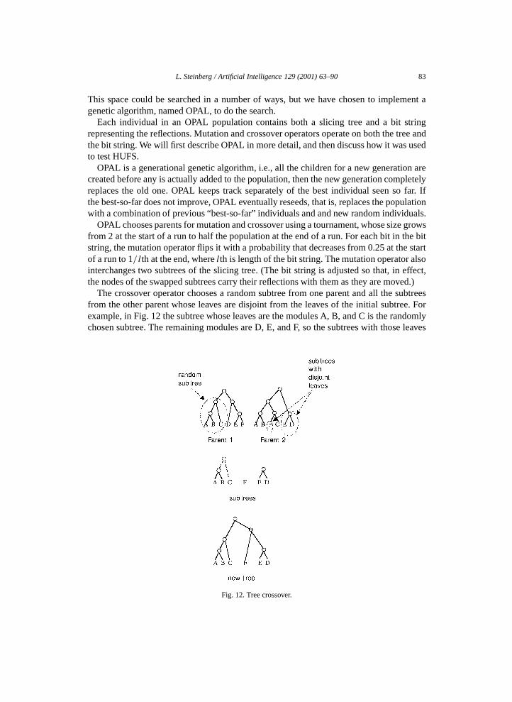
The crossover operator chooses a random subtree from one parent and all the subtreesfrom the other parent whose leaves are disjoint from the leaves of the initial subtree. Forexample, in Fig. 12 the subtree whose leaves are the modules A, B, and C is the randomlychosen subtree. The remaining modules are D, E, and F, so the subtrees with those leaves

Fig. 12. Tree crossover.


Fig. 13. Genetic algorithm on combined space.

Fig. 14. GA on combined space, adjusted score.

are selected from the second parent, and connected randomly to make the new tree, whichis the result of the crossover.

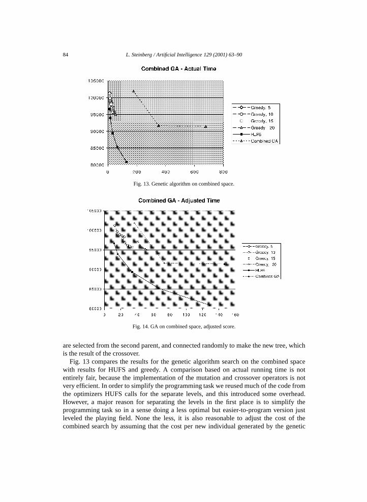
Fig. 13 compares the results for the genetic algorithm search on the combined spacewith results for HUFS and greedy. A comparison based on actual running time is notentirely fair, because the implementation of the mutation and crossover operators is notvery efficient. In order to simplify the programming task we reused much of the code fromthe optimizers HUFS calls for the separate levels, and this introduced some overhead.However, a major reason for separating the levels in the first place is to simplify theprogramming task so in a sense doing a less optimal but easier-to-program version justleveled the playing field. None the less, it is also reasonable to adjust the cost of thecombined search by assuming that the cost per new individual generated by the genetic


algorithm was the same as the cost for the slicing tree optimizer per candidate that itconsidered plus the analogous cost for the reflection optimizer. Fig. 14 shows the resultof making this adjustment.

This is a conservative (low) estimate of the cost of the combined problem because thereis likely to be at least some extra overhead in the combined solver. It also does not take intoaccount the fact that a combined solver is a more complex programming task, especially asthe number of levels grows. In fact, if the optimizers for the various levels are proprietarycode for which source is not available it may be infeasible to construct the combined solverin the first place.

5.2. Trees of GA populations

In order to test the generality of HUFS, we have also applied it to guide the searchthrough a tree whose nodes are populations of a genetic algorithm.

As discussed in the Introduction, it is possible to build a tree in which a node is a savedpopulation from a GA and in which the operator that generates a child population froma parent population is to run the GA for some number of iterations [16]. Because of thestochastic nature of a GA, this is an SG tree, and it can be searched using HUFS.

Our tests used GADO [13], a GA that has a number of features oriented towardsengineering design optimization. The optimization task we used was the conceptual designof a supersonic civil transport aircraft. Each design is represented by 12 real numbers,specifying such things as the wing span and the overall length of the aircraft. A designmust satisfy a number of constraints, including the constraint that it must have room forsome specified number of passengers, and the measure of merit to be optimized is a sumif the estimated weight of the aircraft and the estimated amount of fuel required to flysome specified route. For our tests, a “problem” was specified by giving the number ofpassengers to be carried and the fraction of the route that was to be flown at subsonicspeeds. The “fitness function” optimized by the GA was a weighted sum of the measureof merit and a penalty function for any violated constraints. It takes about half a second ofCPU time to evaluate the fitness of one design. The score of a population was the fitness ofits best individual. The value of a population as a solution was a constant minus the score.

Two changes were made in HUFS for this new problem. First of all, unlike in therectangle placement problem, an alternative population at any level below the root of thetree can be returned as a solution. Therefore, the utility of a population is the maximum ofits utility as computed by HUFS as previously described and its value as a solution.

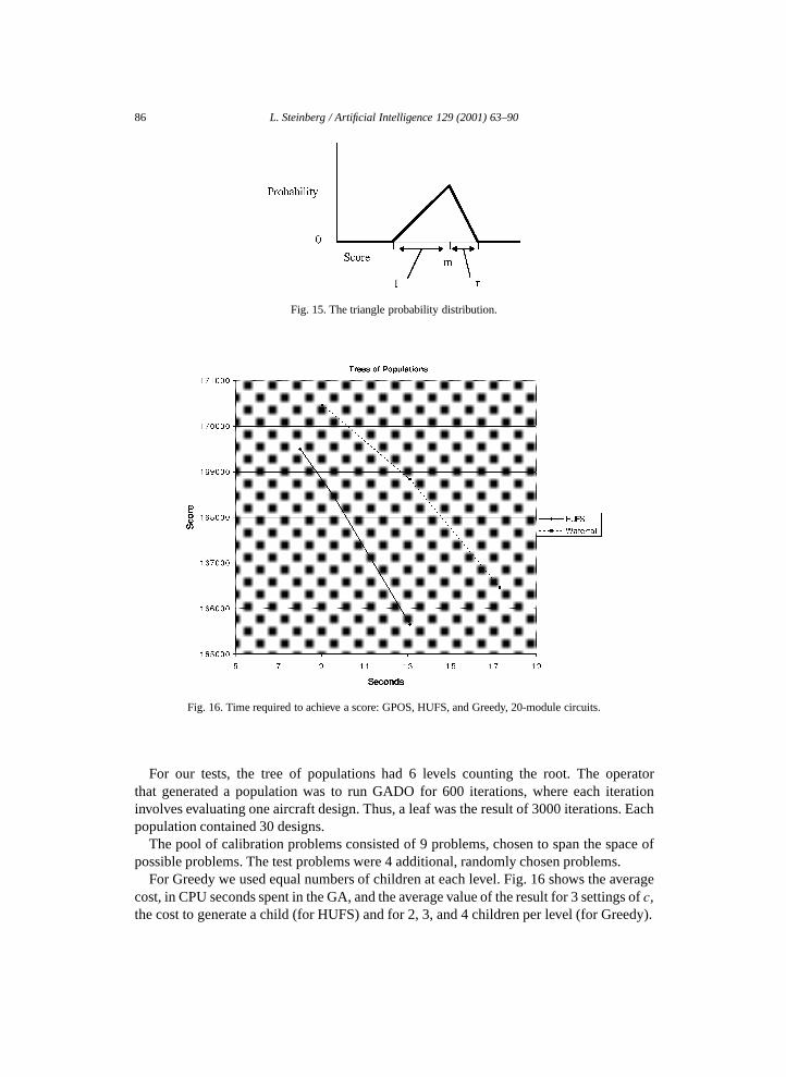
Secondly, the G’s in this domain appear to be somewhat asymmetric, so rather thanmodeling them as normal distributions, we modeled then as “triangle” distributions.A triangle distribution has a probability density function Tl,m,r (s) defined by 3 positivereal parameters, l, m, and r . This density function has its highest value at a score of m andfalls off linearly on either side, reaching a density of 0 at scores of m − l and m + r . (SeeFig. 15.)

The initial estimates of the distributions of parameters l, m, and r were all normaldistributions, with parameters computed in a way similar to the corresponding parametersin the module placement problem.


Fig. 15. The triangle probability distribution.

Fig. 16. Time required to achieve a score: GPOS, HUFS, and Greedy, 20-module circuits.

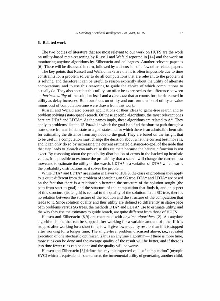
For our tests, the tree of populations had 6 levels counting the root. The operatorthat generated a population was to run GADO for 600 iterations, where each iterationinvolves evaluating one aircraft design. Thus, a leaf was the result of 3000 iterations. Eachpopulation contained 30 designs.

The pool of calibration problems consisted of 9 problems, chosen to span the space ofpossible problems. The test problems were 4 additional, randomly chosen problems.

For Greedy we used equal numbers of children at each level. Fig. 16 shows the averagecost, in CPU seconds spent in the GA, and the average value of the result for 3 settings of c,the cost to generate a child (for HUFS) and for 2, 3, and 4 children per level (for Greedy).


6. Related work

The two bodies of literature that are most relevant to our work on HUFS are the workon utility-based meta-reasoning by Russell and Wefald reported in [14] and the work onmonitoring anytime algorithms by Zilberstein and colleagues. Another relevant paper is[6]. These will be discussed in turn, followed by a discussion of a few other related papers.

The key points that Russell and Wefald make are that it is often impossible due to timeconstraints for a problem solver to do all computations that are relevant to the problem itis solving, and therefore it can be useful to reason explicitly about the utility of alternatecomputations, and to use this reasoning to guide the choice of which computations toactually do. They also note that this utility can often be expressed as the difference betweenan intrinsic utility of the solution itself and a time cost that accounts for the decreased inutility as delay increases. Both our focus on utility and our formulation of utility as valueminus cost of computation time were drawn from this work.

Russell and Wefald also present applications of their ideas to game-tree search and toproblem solving (state-space) search. Of these specific algorithms, the most relevant oneshere are DTA* and LDTA*. As the names imply, these algorithms are related to A*. Theyapply to problems like the 15-Puzzle in which the goal is to find the shortest path through astate space from an initial state to a goal state and for which there is an admissible heuristicfor estimating the distance from any node to the goal. They are based on the insight thatto be useful, a computation must change the decision about what the current best move is,and it can only do so by increasing the current estimated distance-to-goal of the node thatthat step leads to. Search can only raise this estimate because the heuristic function is notexact. By reasoning about the probability distribution of errors in the backed up heuristicvalues, it is possible to estimate the probability that a search will change the current bestmove and to estimate the utility of the search. LDTA* is a variation of DTA* which learnsthe probability distributions as it solves the problem.

While DTA* and LDTA* are similar in flavor to HUFS, the class of problems they applyto is quite different from the problem of searching an SG tree. DTA* and LDTA* are basedon the fact that there is a relationship between the structure of the solution sought (thepath from start to goal) and the structure of the computation that finds it, and an aspectof this structure (its length) is central to the quality of the solution. In an SG tree, there isno relation between the structure of the solution and the structure of the computation thatleads to it. Since solution quality and thus utility are defined so differently in state-spacepath problems versus SG trees, the methods DTA* and LDTA* use to estimate utility, andthe way they use the estimates to guide search, are quite different from those of HUFS.

Hansen and Zilberstein [8,9] are concerned with anytime algorithms [2]. An anytimealgorithm is one that can be stopped after working for a variable amount of time. If it isstopped after working for a short time, it will give lower quality results than if it is stoppedafter working for a longer time. The single-level problem discussed above, i.e., repeatedexecution of one stochastic optimizer, is thus an anytime algorithm—if there is more time,more runs can be done and the average quality of the result will be better, and if there isless time fewer runs can be done and the quality will be worse.

Hansen and Zilberstein [8] define the “myopic expected value of computation” (myopicEVC) which is equivalent in our terms to the incremental utility of generating another child.


Their rule for stopping, stop when myopic EVC is negative, is equivalent to ours. However,Hansen and Zilberstein are concerned with the general case of anytime algorithms (andalso with the cost of the monitoring, which we do not consider), and thus do not derive anymore specific formula for myopic EVC. They also do not consider multi-level systems.

Zilberstein and Russell [21,22] also define a stopping rule similar to ours and prove that,under conditions similar to those that hold in our single-level case, it is optimal.

It is worth noting that while repeated stochastic optimization can be seen as an anytimealgorithm, HUFS as a whole is not an anytime algorithm. If it is stopped before any ground-level design is produced, then it gives no answer at all. Steinberg and Rasheed’s [16] is aninitial report on a version of HUFS that allows for a deadline, that is, a maximum timeby which the result must be available. With deadlines, HUFS does become an anytimealgorithm.

Etzioni [6] describes an approach to a planning problem that is quite different fromour problem here, but he uses a notion called “marginal utility”. Marginal utility is theincremental value divided by the incremental cost, and is analogous to our EIV − c butis based on a model of utility as “return on investment” rather than our model of utilityas “profit”. He also includes an interesting learning component to estimate means ofdistributions for cost and value.

The Stage system by Boyan and Moore [3,4] learns an objective function thatcharacterizes good starting points for a stochastic local search. Like HUFS it attemptsto characterize the results of an entire search by applying an estimator to the initial pointof a search. Stage does not use utilities; rather it estimates the goodness of a search startingpoint based on the kind of problem-specific features that HUFS uses to estimate G.

Tsitsiklis and van Roy [18] develop some results on optimal stopping that are related totime-difference (reinforcement) learning.

7. Conclusions

It is clear from the empirical experiments that, at least on some tasks, HUFS requiressignificantly fewer optimizer runs than Greedy. It also outperforms a method that combinesthe slicing tree and the reflections into a single search space, and searches that space witha genetic algorithm. However, for the longest of the runs, the advantage of HUFS over thecombined method was small.

While HUFS is somewhat complex to implement, we believe it will be useful in manyproblems that require searching an SG tree. We also believe that, since SG trees have beenidentified as a problem class with an effective solution method, there will be a number ofproblems that will be recognized as, or cast into the form of, SG trees. The work on treesof populations demonstrates the potential advantages of doing so.

More generally, this research shows that very useful utility arguments can be made forstochastic methods, and suggests trying to apply utility reasoning in the context of otherstochastic algorithms.

This research also suggests that there may be other significant search tasks which, likehierarchical optimization, have not been studied much in the context of heuristic search,but for which such study would yield fruitful results.


There are at least three directions in which HUFS could be improved. First of all, wehypothesize that if HUFS could model and predict the Child Score Distributions moreaccurately, it could do even better. This suggests that research on the characteristics ofChild Score Distributions of stochastic optimizers, and on learning probability distributionsin general, would be valuable.

Secondly, HUFS requires that the costs of running the optimizers, on the one hand, andthe value function for the resulting designs, on the other hand be expressed in comparableunits. For instance, in the rectangle placement problem this might amount to deciding howmany minutes of CPU time a square micron of chip area is worth. It is not clear that thiscan be easily done in a real-world setting. This relationship between time cost and qualityvalue can be simply thought of as a control knob which determines how long HUFS runsfor and which can be set empirically, but it would be useful to find a way out of having tospecify these parameters in comparable terms.

Finally, it takes a fair amount of computation to generate the calibration data. In manydomains this is justified by the fact that the cost can be amortized by using this samecalibration data for many problems, but further research in ways to minimize this overheadwould be useful.

Hierarchical optimization is ubiquitous in engineering design, and gives rise to searchproblems quite distinct from those traditionally studied. The work presented here is a firststep towards the principled approaches for solving this new class of problems.

Acknowledgements

The work presented here is part of the “Hypercomputing & Design” (HPCD) project,and benefited greatly from both the intellectual and software environments provided byour colleagues on that project. Special thanks also to Professor Robert Berk for hiscontributions on the statistical theory. Thanks are also due to the anonymous reviewersfor a number of useful suggestions.

The work presented here is part of the “Hypercomputing & Design” (HPCD) project;and it is supported (partly) by ARPA under contract DABT-63-93-C-0064 and by NSFunder Grant Number DMI-9813194. The content of the information herein does notnecessarily reflect the position of the Government and official endorsement should notbe inferred.

References

[1] M. Blaize, D. Knight, K. Rasheed, Automated optimal design of two dimensional high speed missile inlets,in: Proc. 36th AIAA Aerospace Sciences Meeting and Exhibit, 1998.

[2] M. Boddy, T. Dean, Deliberation scheduling for problem solving in time-constrained environments,Artificial Intelligence 67 (1994) 245–285.

[3] J.A. Boyan, A.W. Moore, Learning evaluation functions for global optimization and boolean satisfiability,in: Proc. AAAI-98, Madison, WI, 1998.

[4] J.A. Boyan, A.W. Moore, Learning evaluation functions to improve local search, J. Machine Learning Res. 1(2000) 77–112.


[5] Y.S. Chow, H. Robbins, D. Siegmund, Great Expectations: The Theory of Optimal Stopping, HoughtonMifflin, Boston, MA, 1971.

[6] O. Etzioni, Embedding decision-analytic control in a learning architecture, Artificial Intelligence 49 (1991)129–159.

[7] D.E. Goldberg, Genetic Algorithms in Search, Optimization, and Machine Learning, Addison-Wesley,Reading, MA, 1989.

[8] E. Hansen, S. Zilberstein, Monitoring anytime algorithms, SIGART Bulletin (Special Issue on AnytimeAlgorithms and Deliberation Scheduling) 7 (2) (1996) 28–33.

[9] E. Hansen, S. Zilberstein, Monitoring the progress of anytime problem-solving, in: Proc. AAAI-96,Portland, OR, 1996, pp. 1229–1234.

[10] L. Ingber, Adaptive Simulated Annealing (ASA): Lessons learned, Control and Cybernetics 25 (1) (1996)33–54.

[11] R.D. Luce, H. Raiffa, Games and Decisions: Introduction and Critical Survey, Wiley, New York, 1957.[12] Z. Michalewicz, Genetic Algorithms + Data Structures = Evolution Programs, Springer, New York, 1996.[13] K. Rasheed, GADO: A genetic algorithm for continuous design optimization, Technical Report DCS-

TR-352, Department of Computer Science, Rutgers University, New Brunswick, NJ, 1998, Ph.D. Thesis,http://www.cs.rutgers.edu/∼krasheed/thesis.ps.

[14] S. Russell, E. Wefald, Do the Right Thing, MIT Press, Cambridge, MA, 1991.[15] A.N. Shiryayev, Optimal Stopping Rules, Springer, New York, 1978.[16] L. Steinberg, K. Rasheed, Optimization by searching a tree of populations, in: Proc. Genetic and

Evolutionary Computation Conference, 1999.[17] M. Tribus, Rational Descriptions, Decisions and Designs, Pergamon Press, New York, 1969.[18] J.N. Tsitsiklis, B. van Roy, Optimal stopping of Markov processes: Hilbert space theory, approximation

algorithms, and an application to pricing high-dimensional financial derivatives, IEEE Trans. Automat.Control 44 (10) (1999) 1840–1851.

[19] P. William, J. Swartz, Automatic layout of analog and digital mixed macro/standard cell integrated circuits,Ph.D. Thesis, Yale University, New Haven, CT, 1993.

[20] G.-C. Zha, D. Smith, M. Schwabacher, K. Rasheed, A. Gelsey, D. Knight, High performance supersonicmissile inlet design using automated optimization, in: Proc. AIAA Symposium on MultidisciplinaryAnalysis and Optimization-96, 1996.

[21] S. Zilberstein, Operational rationality through compilation of anytime algorithms, Ph.D. Thesis, Universityof California at Berkeley, CA, 1993.

[22] S. Zilberstein, S. Russell, Optimal composition of real-time systems, Artificial Intelligence 82 (1–2) (1996)181–213.

http://www.cs.rutgers.edu/~krasheed/thesis.ps

Documents

Searching stochastically generated multi-abstraction-level design spaces